BasicMacroeconomic

Relationships

9 C H A P T E R

The Income-Consumption and Income-Saving Relationships

• Disposable income is the most important determinant of consumer spending (consumption).

• What is not spent is called saving.

• Disposable Income (DI) = C + S

S = saving

Saving = DI – C

• Note:• (disposable income in Kuwait = personal

income since there is no income tax)• A 45-degree line: each point on the line is

equidistant from the two axes. Therefore, represents all points where consumer spending is equal to disposable income.

• Or each point represent a situation where; C + S = DI

• Any vertical distance from the horizontal axis to the 450 line measures DI

27-4

Income and Consumption

0

1000

2000

3000

4000

5000

6000

7000

8000

9000

10000

0 2000 4000 6000 8000 10000

Con

sum

pti

on (

bil

lion

s of

dol

lars

)

Disposable Income (billions of dollars)

45° Reference LineC=DI

83

8685

84

8889

9190

87

9293

9495

01

9796

9998

00

02

05

03

04

ConsumptionIn 1992

SavingIn 1992

45°

C

Source: Bureau of Economic Analysis

Consumption Schedule

• Reflects the direct consumption-disposable income relationship

• Note: households tend to spend a larger proportion of a small DI than of a larger DI.

The saving schedule

• Reflects the direct relationship between S and DI

• Saving is a smaller proportion of small DI than of a large DI

• Dissaving: when households consume more than their DI. They do that by liquidating their wealth (assets) or by borrowing

Disposable Income Consumption Saving 350 360 -10 370 375 -5 390 390 0 410 405 5 430 420 10 450 435 15 470 450 20 490 465 25 510 480 30 530 495 35 550 510 40

Consumption and Saving Schedules

Co

nsu

mp

tio

nS

avin

g

o

o45

o

C

S

Consumptionschedule

Savingschedule

C

S

Disposable Income

Disposable Income

SAVING

SAVING

DISSAVING

DISSAVING

MPC = Slope of C

MPS = Slope of S

MPC + MPS = 1

CONSUMPTION AND SAVING

Break even income: • The income level at which households plan

to consume their entire income, (C=DI).• At break even:Consumption schedule cuts the 450 line.- Saving schedule cuts the horizontal axis . - Saving = zero- APC = 1- APS = zero

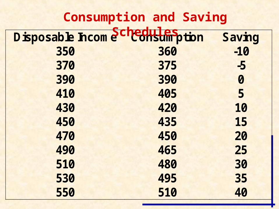
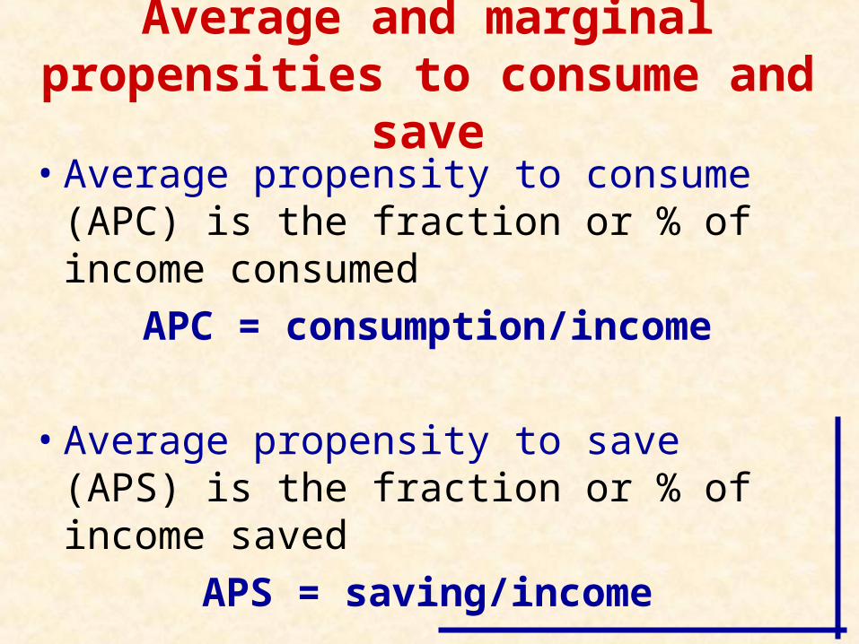
Consumption and Saving(1)

Level ofOutput

AndIncome

(GDP=DI)

(2)Consump-

tion(C)

(3)Saving (S)

(1) – (2)

(4)Average

Propensityto Consume

(APC)(2)/(1)

(5)Average

Propensityto Save(APS)(3)/(1)

(6)Marginal

Propensityto Consume

(MPC)Δ(2)/Δ(1)

(7)Marginal

Propensityto Save(MPS)

Δ(3)/Δ(1)

(1) $370

(2) 390

(3) 410

(4) 430

(5) 450

(6) 470

(7) 490

(8) 510

(9) 530

(10) 550

$375

390

405

420

435

450

465

480

495

510

$-5

0

5

10

15

20

25

30

35

40

1.01

1.00

.99

.98

.97

.96

.95

.94

.93

.93

-.01

.00

.01

.02

.03

.04

.05

.06

.07

.07

.75

.75

.75

.75

.75

.75

.75

.75

.75

.25

.25

.25

.25

.25

.25

.25

.25

.25

MPC + MPS = 1 MPC and MPS measure slopes

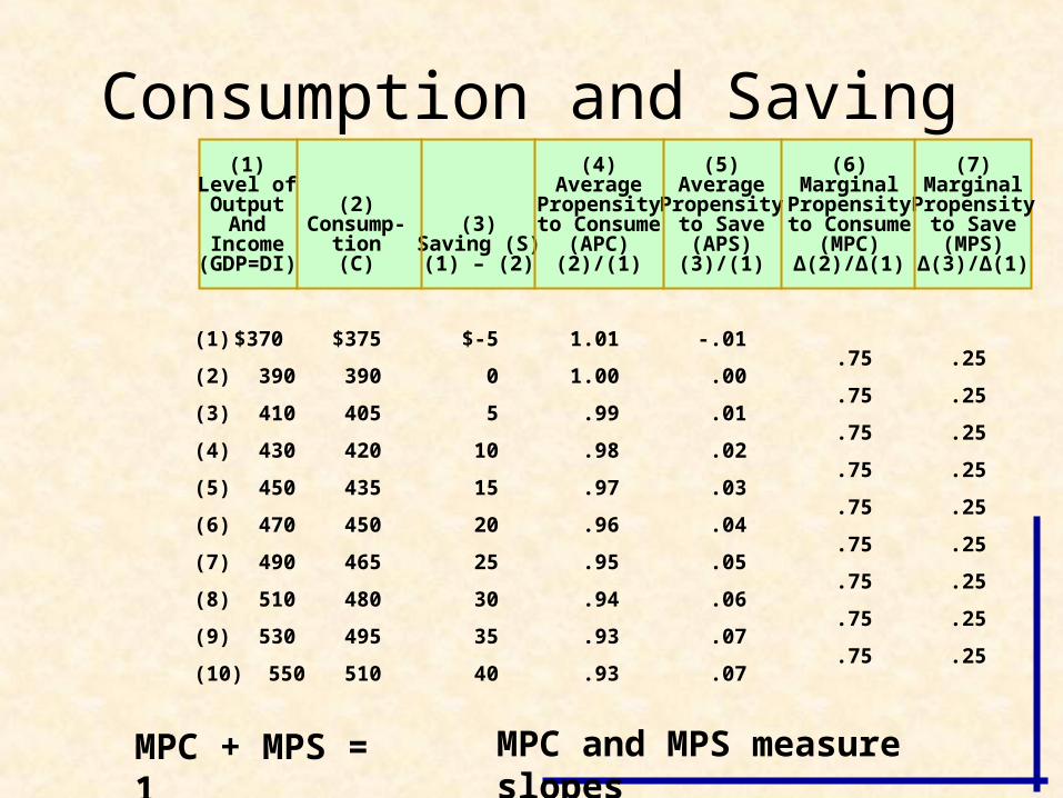
Average and marginal propensities to consume and save

• Average propensity to consume (APC) is the fraction or % of income consumed

APC = consumption/income

• Average propensity to save (APS) is the fraction or % of income saved

APS = saving/income

• Marginal propensity to consume (MPC) is the fraction or proportion of any change in income that is consumed

MPC = change in consumption/change in income

• Marginal propensity to save (MPS) is the fraction or proportion of any change in income that is saved

MPS = change in saving/change in income

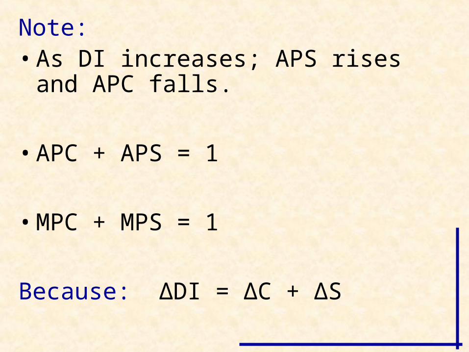
Note:• As DI increases; APS rises and APC falls.

• APC + APS = 1

• MPC + MPS = 1

Because: ∆DI = ∆C + ∆S

Non-income determinants of consumption

1. Wealth: An increase in wealth shifts the consumption schedule up and saving schedule down.

Wealth Effects: when assets boast, households feel wealthy, they save less and consumer more, and vice versa.

2. Expectations: Changes in expected future prices or wealth can affect consumption spending today.

3.Real interest rates: Declining interest rates increase the incentive to borrow and consume, and reduce the incentive to save. Because many household expenditures are not interest sensitive – the light bill, groceries, etc. – the effect of interest rate changes on spending are modest.

4.Household debt: Lower debt levels shift consumption schedule up and saving schedule down. But if debt is too high, they will reduce their consumption to pay off some of their loans.

Terminology, shifts and stability

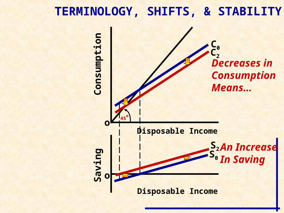
1. Terminology: Movement from one point to another on a given schedule is called a change in amount consumed; a shift in the schedule is called a change in consumption schedule.

2. Schedule shifts: Consumption and saving schedules will always shift in opposite directions unless a shift is caused by a tax change (move together).

3. Stability: Economists believe that consumption and saving schedules are generally stable unless deliberately shifted by government action.

Co

nsu

mp

tio

nS

avin

g

o

o45

o

C0

S0

Disposable Income

Disposable Income

C1

S1

TERMINOLOGY, SHIFTS, & STABILITY

Increases inConsumptionMeans…

A DecreaseIn Saving

Co

nsu

mp

tio

nS

avin

g

o

o45

o

C0

S0

Disposable Income

Disposable Income

C2

S2

TERMINOLOGY, SHIFTS, & STABILITY

Decreases inConsumptionMeans…

An IncreaseIn Saving

27-19

Average Propensity to Consume

Source: Statistical Abstract of the United States, 2006

Selected Nations, with respect to GDP, 2006

United States

Canada

United Kingdom

Japan

Germany

Netherlands

Italy

France

.80 .85 .90 .95 1.00

The Interest Rate – Investment Relationship • Investment consists of spending on new plants, capital

equipment, machinery, inventories, construction, etc.

• The investment decision weighs marginal benefits (r) and marginal costs (i).

1. Expected Rate of Return, r: This is marginal benefit of investment.

• Expected Rate of Return = expected profit/cost of capital

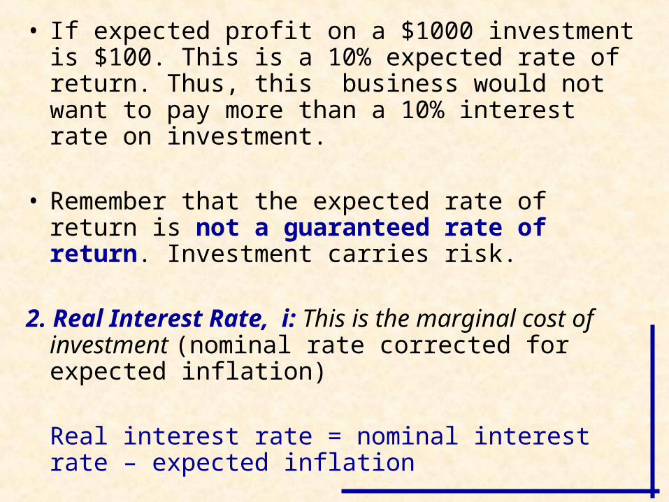
• If expected profit on a $1000 investment is $100. This is a 10% expected rate of return. Thus, this business would not want to pay more than a 10% interest rate on investment.

• Remember that the expected rate of return is not a guaranteed rate of return. Investment carries risk.

2. Real Interest Rate, i: This is the marginal cost of investment (nominal rate corrected for expected inflation)

Real interest rate = nominal interest rate – expected inflation

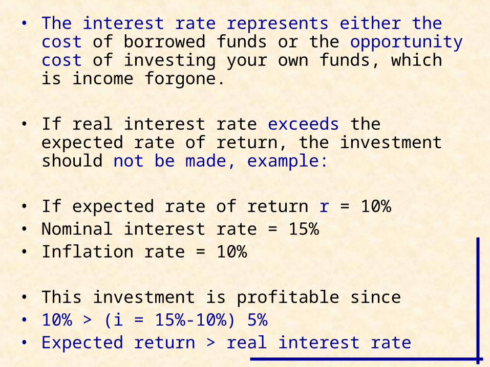
• The interest rate represents either the cost of borrowed funds or the opportunity cost of investing your own funds, which is income forgone.

• If real interest rate exceeds the expected rate of return, the investment should not be made, example:

• If expected rate of return r = 10%• Nominal interest rate = 15%• Inflation rate = 10%

• This investment is profitable since• 10% > (i = 15%-10%) 5%• Expected return > real interest rate

Interest rates

Expected rate of return

Cumulative investment

16% 0

14% 5

12% 10

10% 15

8% 20

6% 25

4% 30

2% 35

0% 40

Investment demand curve

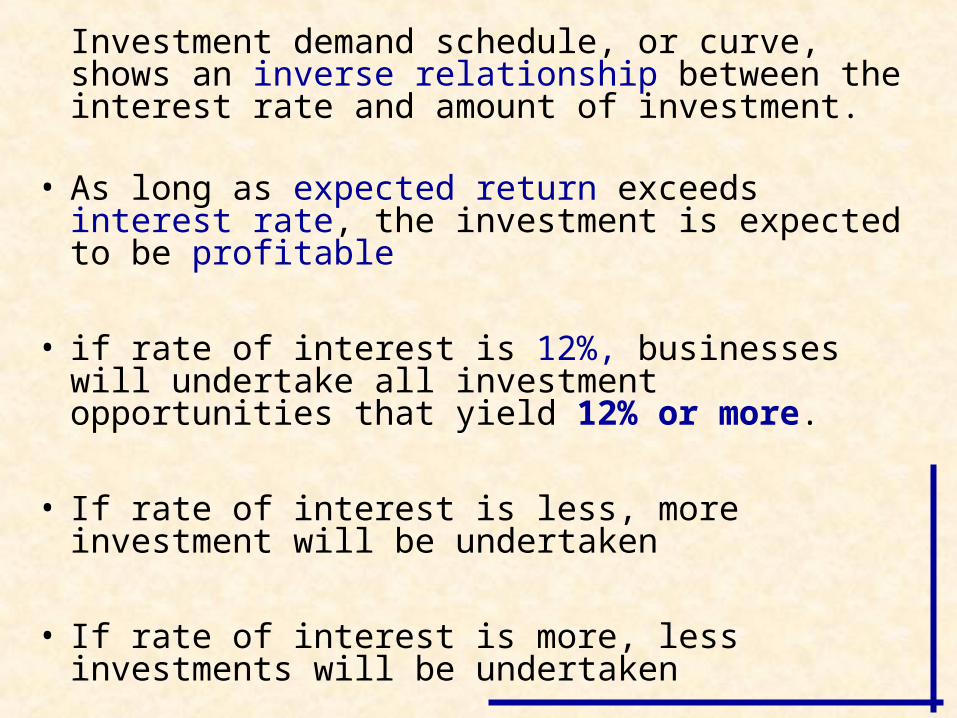
Investment demand schedule, or curve, shows an inverse relationship between the interest rate and amount of investment.

• As long as expected return exceeds interest rate, the investment is expected to be profitable

• if rate of interest is 12%, businesses will undertake all investment opportunities that yield 12% or more.

• If rate of interest is less, more investment will be undertaken

• If rate of interest is more, less investments will be undertaken

Investment (billions of dollars)

Ex

pe

cte

d r

ate

of

retu

rn,

r,a

nd

inte

res

t ra

te, i

(pe

rce

nts

) 16

14

12

10

8

6

4

2

0

INVESTMENTDEMAND

CURVE

5 10 15 20 25 30 35 40

I D

Interest Rate – InvestmentRelationship

Shifts of investment demand

1. Acquisition, Maintenance, and Operating Costs: Initial costs of capital, operating costs and maintenance affect the expected rate of return

– When they fall, prospective investment projects increase (shift to the RHS)

– When they increase, prospective investment projects decrease (shift to the LHS)

2. Business Taxes

When tax increases, expected (after tax) return decreases, shifts the investment curve to the LHS and vice versa.

3. Technological Change

Technological progress (more efficient machines). Technological change often involves lower costs, which would increase expected returns and stimulates investment (shifts the investment curve to the RHS, and vice versa).

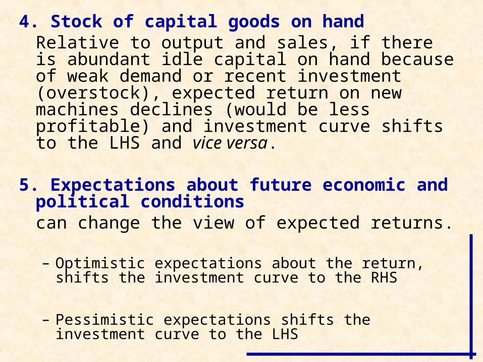
4. Stock of capital goods on handRelative to output and sales, if there is abundant idle capital on hand because of weak demand or recent investment (overstock), expected return on new machines declines (would be less profitable) and investment curve shifts to the LHS and vice versa.

5. Expectations about future economic and political conditionscan change the view of expected returns.

– Optimistic expectations about the return, shifts the investment curve to the RHS

– Pessimistic expectations shifts the investment curve to the LHS

Instability of investmentInvestment schedule is unstable, it shifts upward or downward quite often. Investment is the most volatile component of total spending.

Reasons for instability of investment

1. Durability of capital and variability of expectations

Within limits, purchases of capital goods are discretionary and therefore, can be postponed. Optimism about future may prompt firms to replace older capital. Pessimism about the future lead to small investment as firms repair old capital.

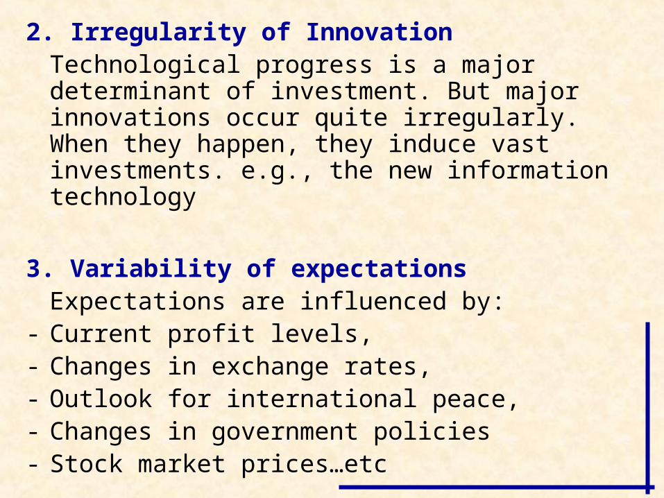
2. Irregularity of InnovationTechnological progress is a major determinant of investment. But major innovations occur quite irregularly. When they happen, they induce vast investments. e.g., the new information technology

3. Variability of expectationsExpectations are influenced by:

- Current profit levels, - Changes in exchange rates,- Outlook for international peace, - Changes in government policies- Stock market prices…etc

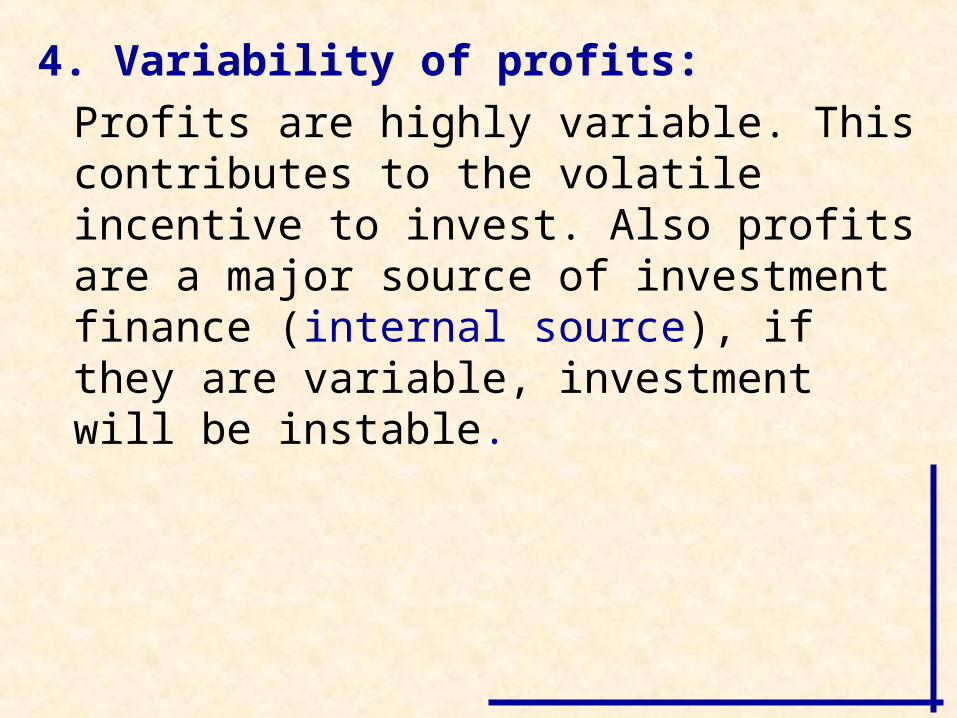
4. Variability of profits:

Profits are highly variable. This contributes to the volatile incentive to invest. Also profits are a major source of investment finance (internal source), if they are variable, investment will be instable.

27-32

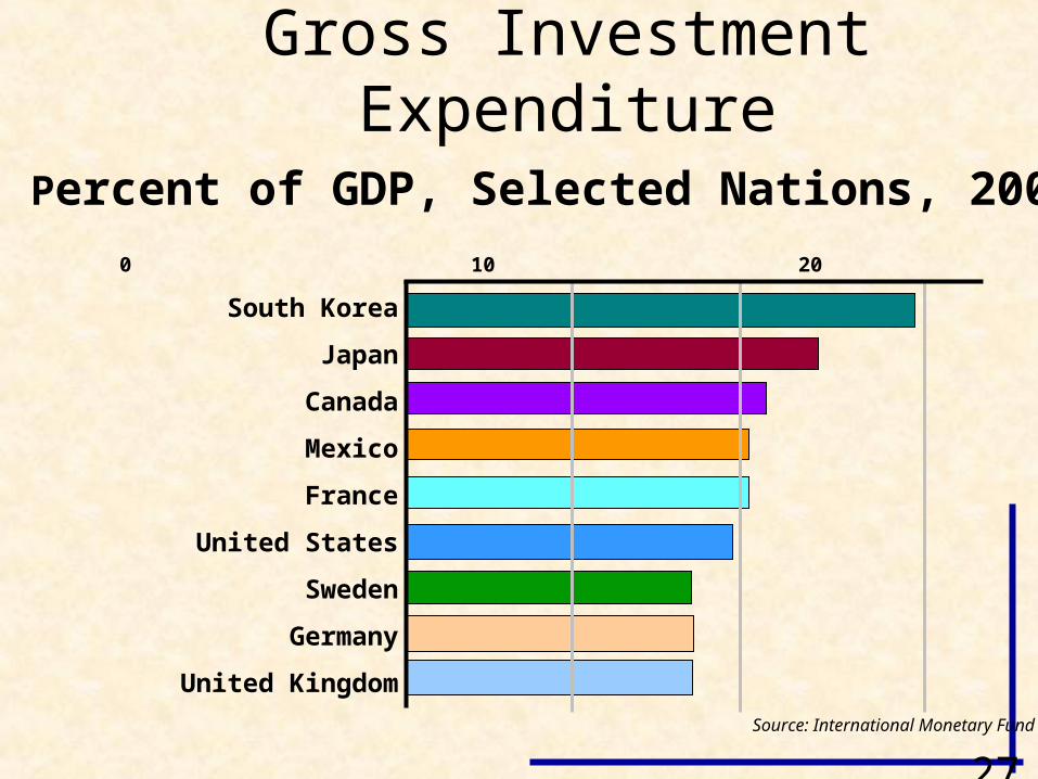
Gross Investment Expenditure

Source: International Monetary Fund

Percent of GDP, Selected Nations, 2006

South Korea

Japan

Canada

Mexico

France

United States

Sweden

Germany

United Kingdom

0 10 20 30

Volatility of Investment

Source: Bureau of Economic Analysis

27-33

The Multiplier Effect• Changes in spending ripple through the economy to

generate even larger changes in real GDP. This is called the multiplier effect.

Multiplier = change in real GDP / initial change in spending.

Alternatively, it can be rearranged to read

Change in real GDP = initial change in spending × multiplier.

Three points to remember about the multiplier:

a. The initial change in spending is usually associated with investment because it is so volatile.

b. The initial change refers to an upward shift or downward shift in the aggregate expenditures schedule due to a change in one of its components, like investment.

c. The multiplier works in both directions (up or down).

Rationale: The multiplier is based on two facts

1. The economy has continuous flows of expenditures and income—a ripple effect—in which income received by Ali comes from money spent by Ahmad. Ahmad’s income, in turn, came from money spent by Said, and so forth.

2. Any change in income will cause both consumption and saving to vary in the same direction as the initial change in income, and by a fraction of that change.

a. The fraction of the change in income that is spent is called the marginal propensity to consume (MPC).

b. The fraction of the change in income that is saved is called the marginal propensity to save (MPS).

Changein GDP =Multiplier x initial change

in spending

THE MULTIPLIER EFFECT

Multiplier =Change in Real GDP

Initial Change in Spending

For Example…

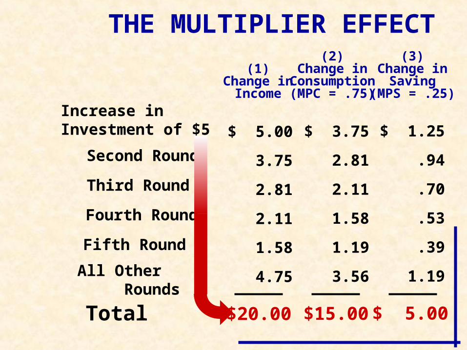
THE MULTIPLIER EFFECT

Increase in Investment of $5

Second Round

Third Round

Fourth Round

Fifth Round

All Other Rounds

Total

(1)Change in

Income

(2)Change in

Consumption(MPC = .75)

(3)Change in

Saving(MPS = .25)

$ 5.00

3.75

2.81

2.11

1.58

4.75

$ 3.75

2.81

2.11

1.58

1.19

3.56

$ 1.25

.94

.70

.53

.39

1.19

$20.00 $15.00 $ 5.00

Change inGDP = Multiplier x initial change

in spending

Multiplier = or 1

MPS

1

1 - MPC

THE MULTIPLIER EFFECT

Inverse relationship between: Multiplier & MPS

Multiplier Effect and the Marginal Propensities

THE MULTIPLIER EFFECT

.9

.8

.75

.67

.5

10

5

4

3

2

MPC Multiplier

MPC and the Multiplier

• The size of the MPC and the multiplier are directly related.

• The significance of the multiplier is that a small change in investment plans or consumption-saving plans can trigger a much larger change in the equilibrium level of GDP.

• The simple multiplier given above can be generalized to include other “leakages” from the spending flow besides savings. For example, the actual multiplier is derived by including taxes and imports as well as savings in the equation. In other words, the denominator is the fraction of a change in income not spent on domestic output.