Embed Size (px)
Citation preview
Basic linear regression and multiple regression
Psych 437 - Fraley
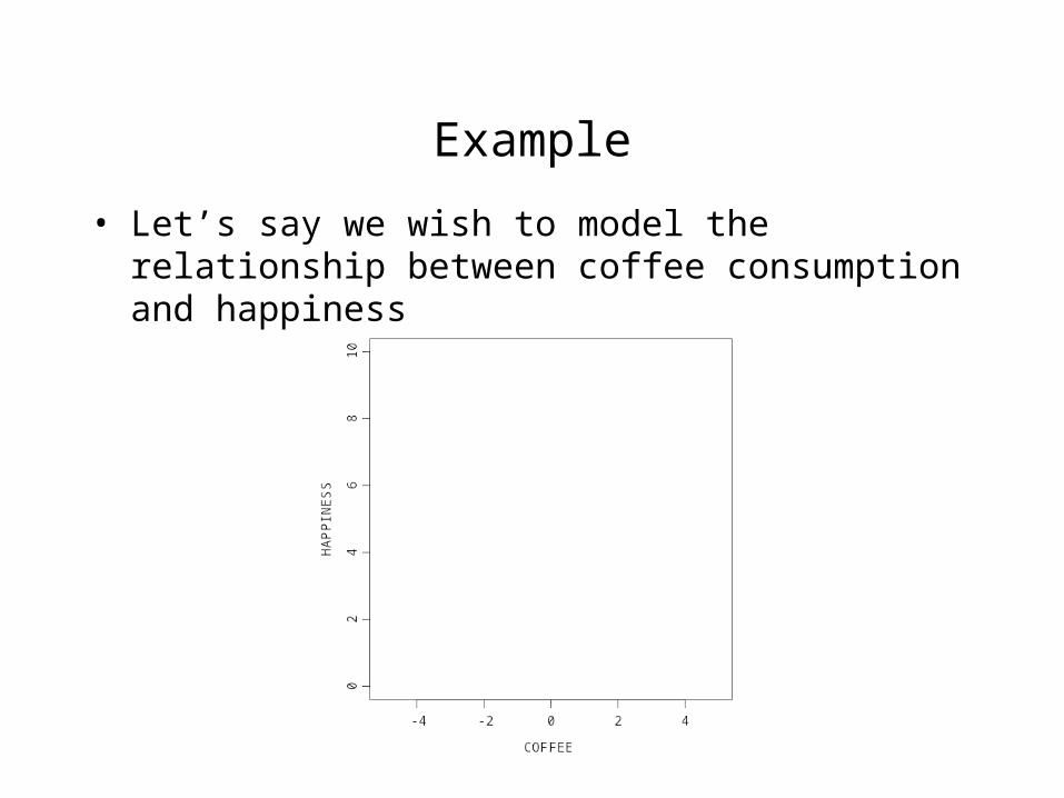
Example
• Let’s say we wish to model the relationship between coffee consumption and happiness
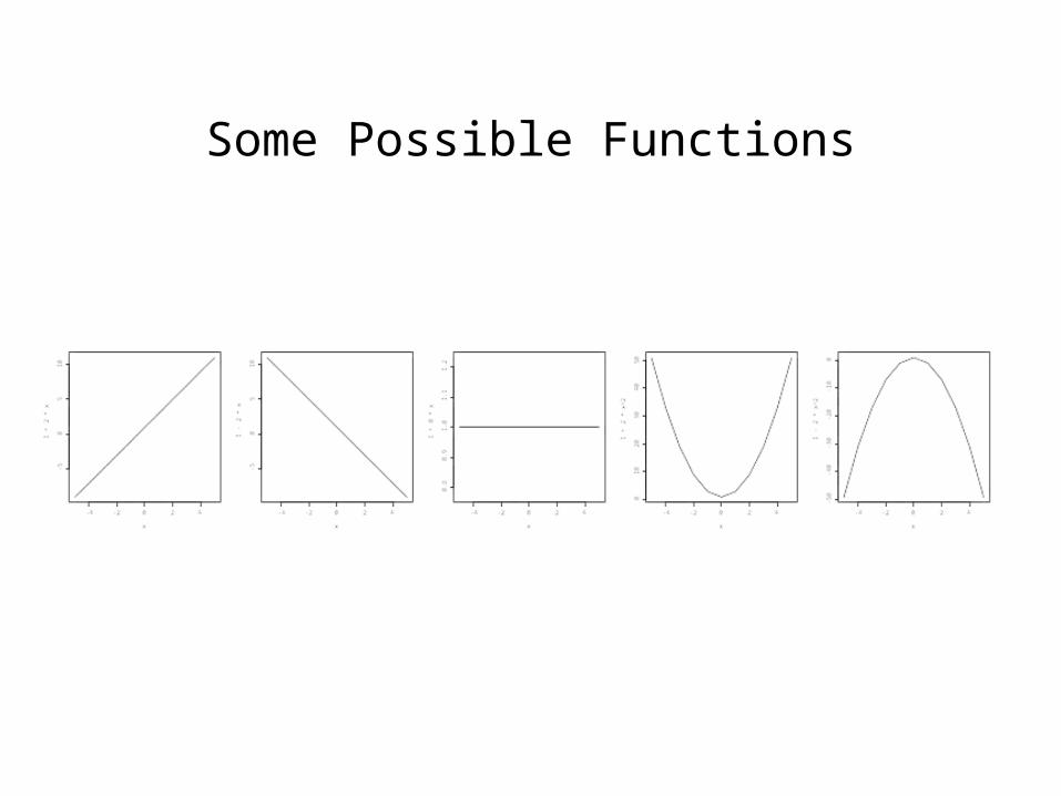
Some Possible Functions
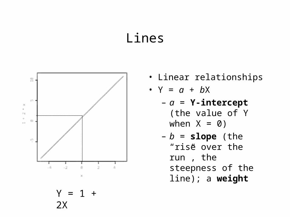
Lines
• Linear relationships
• Y = a + bX
– a = Y-intercept (the value of Y when X = 0)
– b = slope (the “rise over the run”, the steepness of the line); a weight
Y = 1 + 2X
Lines and intercepts
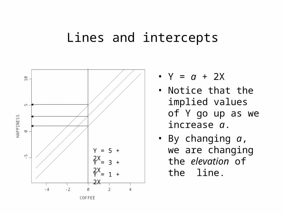
• Y = a + 2X
• Notice that the implied values of Y go up as we increase a.
• By changing a, we are changing the elevation of the line.
Y = 1 + 2X
Y = 3 + 2X
Y = 5 + 2X
Lines and slopes
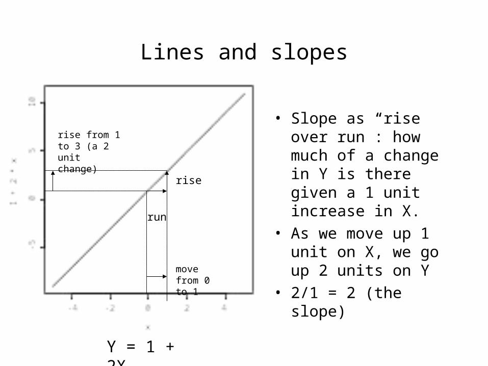
• Slope as “rise over run”: how much of a change in Y is there given a 1 unit increase in X.
• As we move up 1 unit on X, we go up 2 units on Y
• 2/1 = 2 (the slope)
Y = 1 + 2X
run
rise
move from 0 to 1
rise from 1 to 3 (a 2 unit change)
Lines and slopes
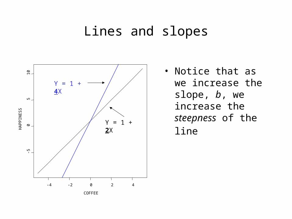
• Notice that as we increase the slope, b, we increase the steepness of the line
COFFEE
HA
PP
INE
SS
-4 -2 0 2 4
-50
510
Y = 1 + 2X
Y = 1 + 4X
COFFEE
HA
PP
INE
SS
-4 -2 0 2 4
-50
51
0
Lines and slopes
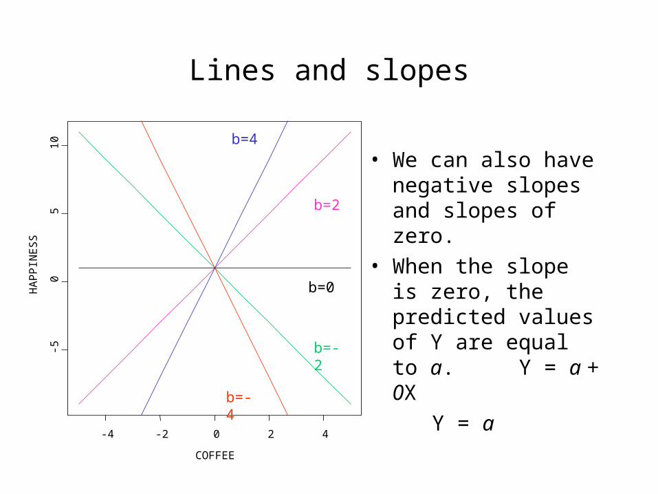
• We can also have negative slopes and slopes of zero.
• When the slope is zero, the predicted values of Y are equal to a.
Y = a + 0X
Y = a
b=2
b=4
b=0
b=-2
b=-4
Other functions
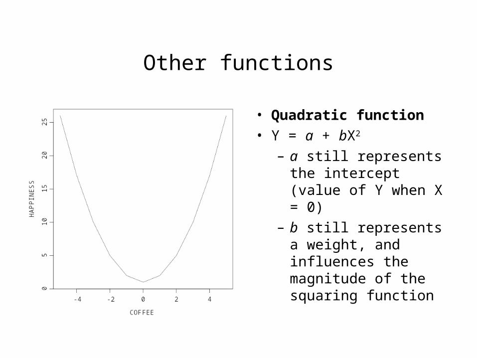
• Quadratic function
• Y = a + bX2
– a still represents the intercept (value of Y when X = 0)
– b still represents a weight, and influences the magnitude of the squaring function
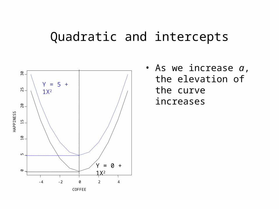
Quadratic and intercepts
• As we increase a, the elevation of the curve increases
COFFEE
HA
PP
INE
SS
-4 -2 0 2 4
05
1015
2025
30
Y = 0 + 1X2
Y = 5 + 1X2
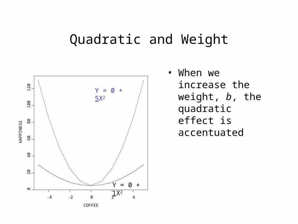
Quadratic and Weight
• When we increase the weight, b, the quadratic effect is accentuated
COFFEE
HA
PP
INE
SS
-4 -2 0 2 4
020
4060
8010
012
0
Y = 0 + 1X2
Y = 0 + 5X2
COFFEE
HA
PP
INE
SS
-4 -2 0 2 4
-100
-50
050
100
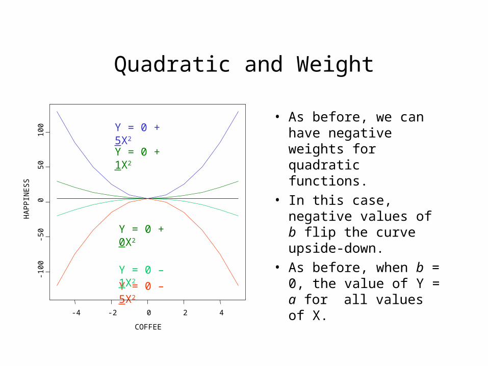
Quadratic and Weight
• As before, we can have negative weights for quadratic functions.
• In this case, negative values of b flip the curve upside-down.
• As before, when b = 0, the value of Y = a for all values of X.Y = 0 – 5X2
Y = 0 – 1X2
Y = 0 + 1X2
Y = 0 + 5X2
Y = 0 + 0X2
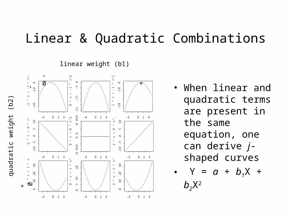
Linear & Quadratic Combinations
• When linear and quadratic terms are present in the same equation, one can derive j-shaped curves
• Y = a + b1X + b2X2
linear weight (b1)
- 0 +
quad
rati
c w
eigh
t (b2
)
+
0
-
Some terminology
• When the relation between variables are expressed in this manner, we call the relevant equation(s) mathematical models
• The intercept and weight values are called parameters of the model.
• Although one can describe the relationship between two variables in the way we have done here, for now on we’ll assume that our models are causal models, such that the variable on the left-hand side of the equation is assumed to be caused by the variable(s) on the right-hand side.
Terminology
• The values of Y in these models are often called predicted values, sometimes abbreviated as Y-hat or . Why? They are the values of Y that are implied by the specific parameters of the model.
Y
Estimation
• Up to this point, we have assumed that our models are correct.
• There are two important issues we need to deal with, however:
– Assuming the basic model is correct (e.g., linear), what are the correct parameters for the model?
– Is the basic form of the model correct? That is, is a linear, as opposed to a quadratic, model the appropriate model for characterizing the relationship between variables?
Estimation
• The process of obtaining the correct parameter values (assuming we are working with the right model) is called parameter estimation.
Parameter Estimation example
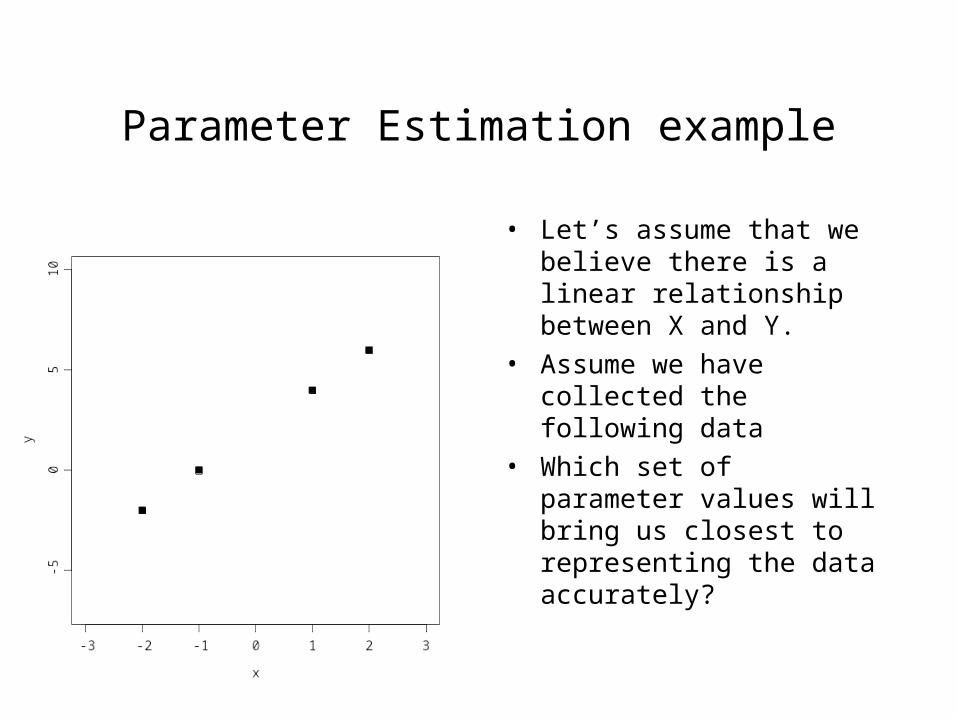
• Let’s assume that we believe there is a linear relationship between X and Y.
• Assume we have collected the following data
• Which set of parameter values will bring us closest to representing the data accurately?
Estimation example
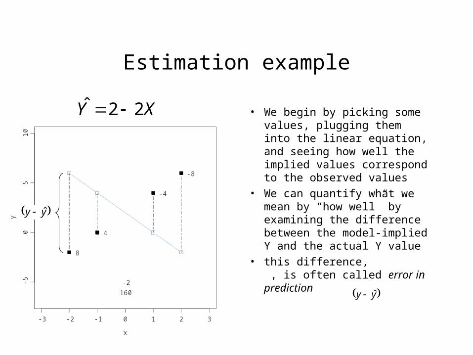
• We begin by picking some values, plugging them into the linear equation, and seeing how well the implied values correspond to the observed values
• We can quantify what we mean by “how well” by examining the difference between the model-implied Y and the actual Y value
• this difference, , is often called error in prediction
XY 22ˆ
yy ˆ
yy ˆ
Estimation example
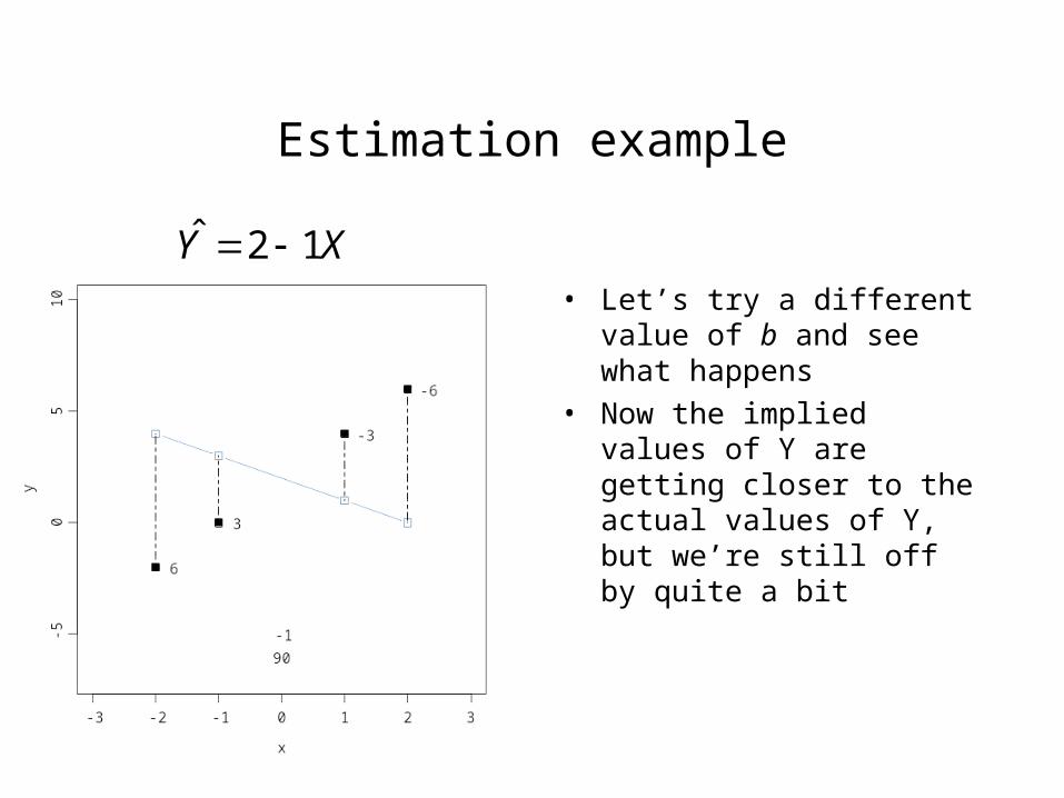
• Let’s try a different value of b and see what happens
• Now the implied values of Y are getting closer to the actual values of Y, but we’re still off by quite a bit
XY 12ˆ
Estimation example
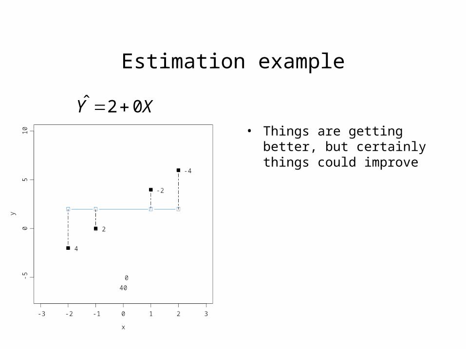
• Things are getting better, but certainly things could improve
XY 02ˆ
Estimation example
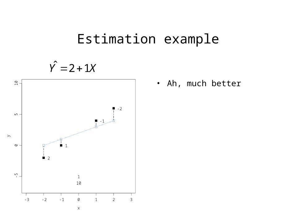
• Ah, much better
XY 12ˆ
Estimation example
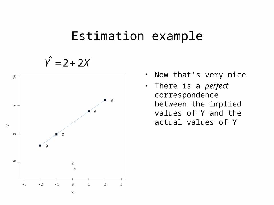
• Now that’s very nice
• There is a perfect correspondence between the implied values of Y and the actual values of Y
XY 22ˆ
Estimation example
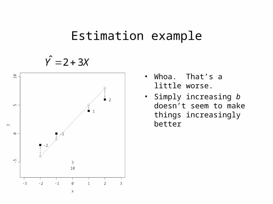
• Whoa. That’s a little worse.
• Simply increasing b doesn’t seem to make things increasingly better
XY 32ˆ
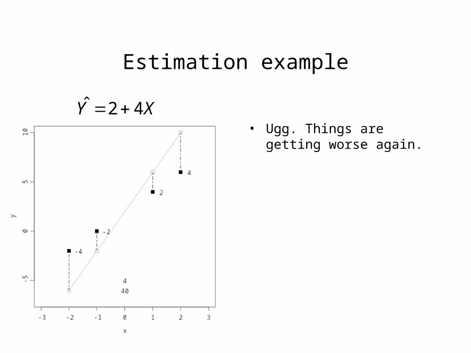
Estimation example
• Ugg. Things are getting worse again.
XY 42ˆ
Parameter Estimation example
• Here is one way to think about what we’re doing:
– We are trying to find a set of parameter values that will give us a small—the smallest—discrepancy between the predicted Y values and the actual values of Y.
• How can we quantify this?
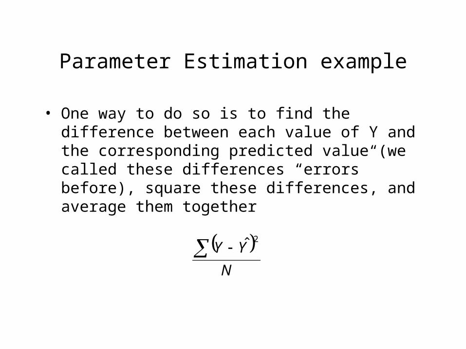
Parameter Estimation example
• One way to do so is to find the difference between each value of Y and the corresponding predicted value (we called these differences “errors” before), square these differences, and average them together
N
YY 2ˆ
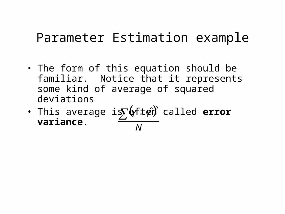
Parameter Estimation example
• The form of this equation should be familiar. Notice that it represents some kind of average of squared deviations
• This average is often called error variance.
N
YY 2ˆ
Parameter Estimation example
• In estimating the parameters of our model, we are trying to find a set of parameters that minimizes the error variance. In other words, we want to be as small as it possibly can be.
• The process of finding this minimum value is called least-squares estimation.
N
YY 2ˆ
Parameter Estimation example
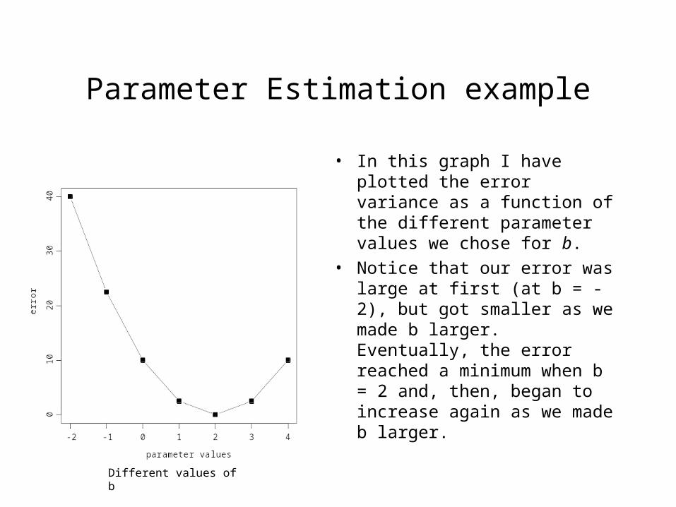
• In this graph I have plotted the error variance as a function of the different parameter values we chose for b.
• Notice that our error was large at first (at b = -2), but got smaller as we made b larger. Eventually, the error reached a minimum when b = 2 and, then, began to increase again as we made b larger.
Different values of b
Parameter Estimation example
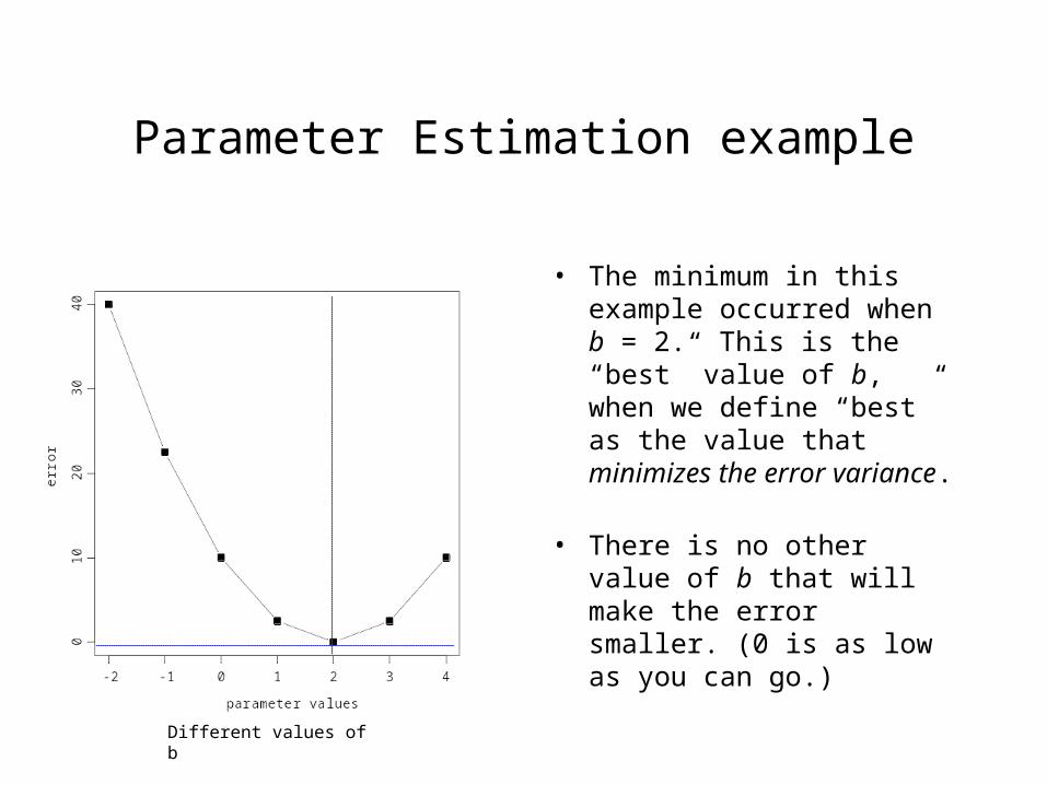
• The minimum in this example occurred when b = 2. This is the “best” value of b, when we define “best” as the value that minimizes the error variance.
• There is no other value of b that will make the error smaller. (0 is as low as you can go.)
Different values of b
Ways to estimate parameters
• The method we just used is sometimes called the brute force or gradient descent method to estimating parameters.– More formally, gradient decent involves starting with
viable parameter value, calculating the error using slightly different value, moving the best guess parameter value in the direction of the smallest error, then repeating this process until the error is as small as it can be.
• Analytic methods– With simple linear models, the equation is so simple
that brute force methods are unnecessary.
Analytic least-squares estimation
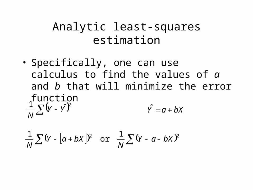
• Specifically, one can use calculus to find the values of a and b that will minimize the error function
2ˆ1
YYN
bXaY ˆ
22 1or
1bXaY
NbXaY
N
Analytic least-squares estimation
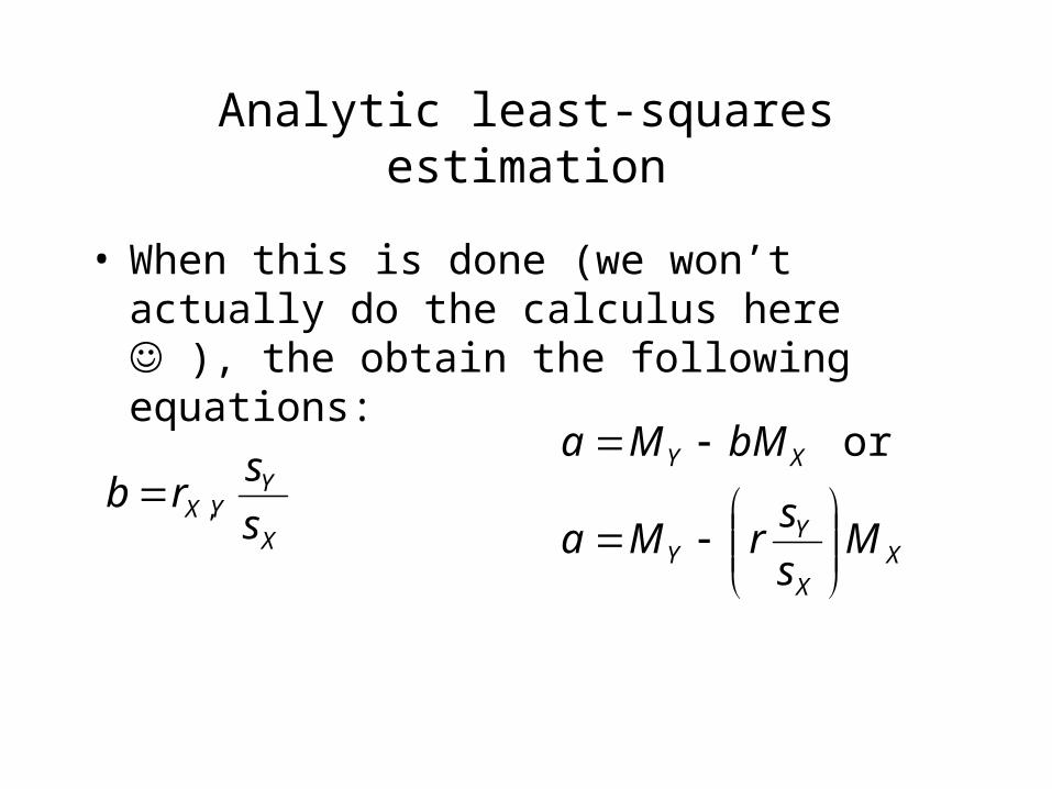
• When this is done (we won’t actually do the calculus here ), the obtain the following equations:
XX
YY
XY
Ms
srMa
bMMa
or
X
YYX s
srb ,
Analytic least-squares estimation
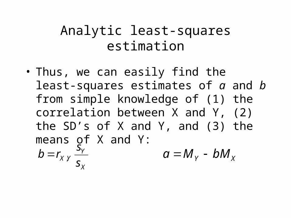
• Thus, we can easily find the least-squares estimates of a and b from simple knowledge of (1) the correlation between X and Y, (2) the SD’s of X and Y, and (3) the means of X and Y:
X
YYX s
srb , XY bMMa
A neat fact
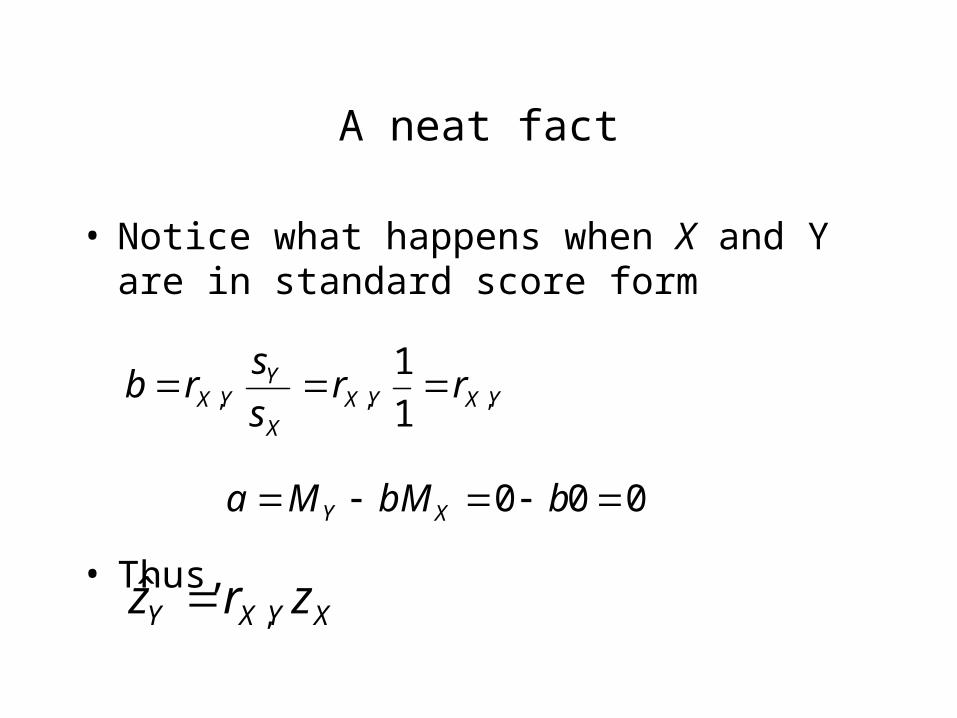
• Notice what happens when X and Y are in standard score form
• Thus,
000 bbMMa XY
YXYXX
YYX rr
s
srb ,,, 1
1
XYXY zrz ,ˆ
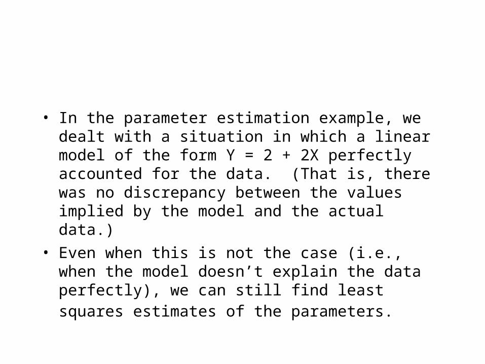
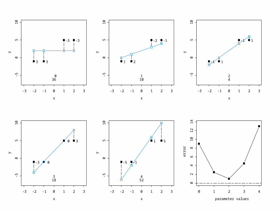
• In the parameter estimation example, we dealt with a situation in which a linear model of the form Y = 2 + 2X perfectly accounted for the data. (That is, there was no discrepancy between the values implied by the model and the actual data.)
• Even when this is not the case (i.e., when the model doesn’t explain the data perfectly), we can still find least squares estimates of the parameters.
x
y
-3 -2 -1 0 1 2 3
-50
51
0
3 3
-3 -3
036
xy
-3 -2 -1 0 1 2 3
-50
51
0
1 2
-2 -1
110
x
y
-3 -2 -1 0 1 2 3
-50
51
0
-1 1
-1 1
24
x
y
-3 -2 -1 0 1 2 3
-50
51
0
-3 0
0 3
318
x
y
-3 -2 -1 0 1 2 3
-50
51
0
-5 -1
1 5
452
parameter values
err
or
0 1 2 3 40
24
68
10
12
14
Error Variance
• In this example, the value of b that minimizes the error variance is also 2. However, even when b = 2, there are discrepancies between the predictions entailed by the model and the actual data values.
• Thus, the error variance becomes not only a way to estimate parameters, but a way to evaluate the basic model itself.
R-squared
• In short, when the model is a good representation of the relationship between Y and X, the error variance of the model should be relatively low.
• This is typically quantified by an index called the multiple R or the squared version of it, R2.
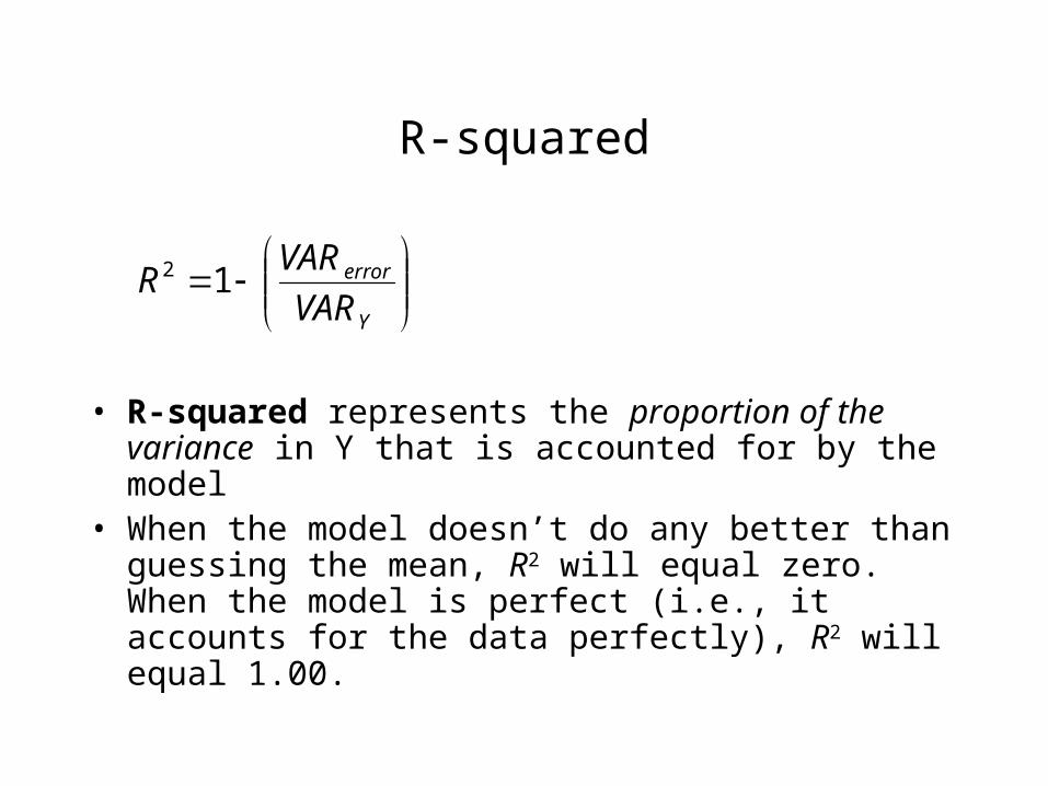
R-squared
• R-squared represents the proportion of the variance in Y that is accounted for by the model
• When the model doesn’t do any better than guessing the mean, R2 will equal zero. When the model is perfect (i.e., it accounts for the data perfectly), R2 will equal 1.00.
Y
error
VAR
VARR 12
Neat fact
• When dealing with a simple linear model with one X, R2 is equal to the correlation of X and Y, squared.
• Why? Keep in mind that R2 is in a standardized metric in virtue of having divided the error variance by the variance of Y. Previously, when working with standardized scores in simple linear regression equations, we found that the parameter b is equal to r. Since b is estimated via least-squares techniques, it is directly related to R2.
Why is R2 useful?
• R2 is useful because it is a standard metric for interpreting model fit.
– It doesn’t matter how large the variance of Y is because everything is evaluated relative to the variance of Y
– Set end-points: 1 is perfect and 0 is as bad as a model can be.
Multiple Regression
• In many situations in personality psychology we are interested in modeling Y not only as a function of a single X variable, but potentially many X variables.
• Example: We might attempt to explain variation in academic achievement as a function of SES and maternal education.
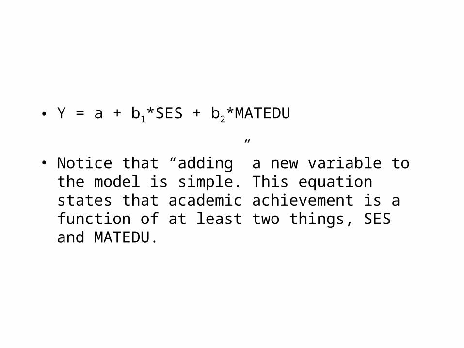
• Y = a + b1*SES + b2*MATEDU
• Notice that “adding” a new variable to the model is simple. This equation states that academic achievement is a function of at least two things, SES and MATEDU.
• However, what the regression coefficients now represent is not merely the change in Y expected given a 1 unit increase in X. They represent the change in Y given a 1-unit change in X assuming all the other variables in the equation equal zero.
• In other words, these coefficients are kind of like partial correlations (technically, they are called semi-partial correlations). We’re statistically controlling SES when estimating the effect of MATEDU.
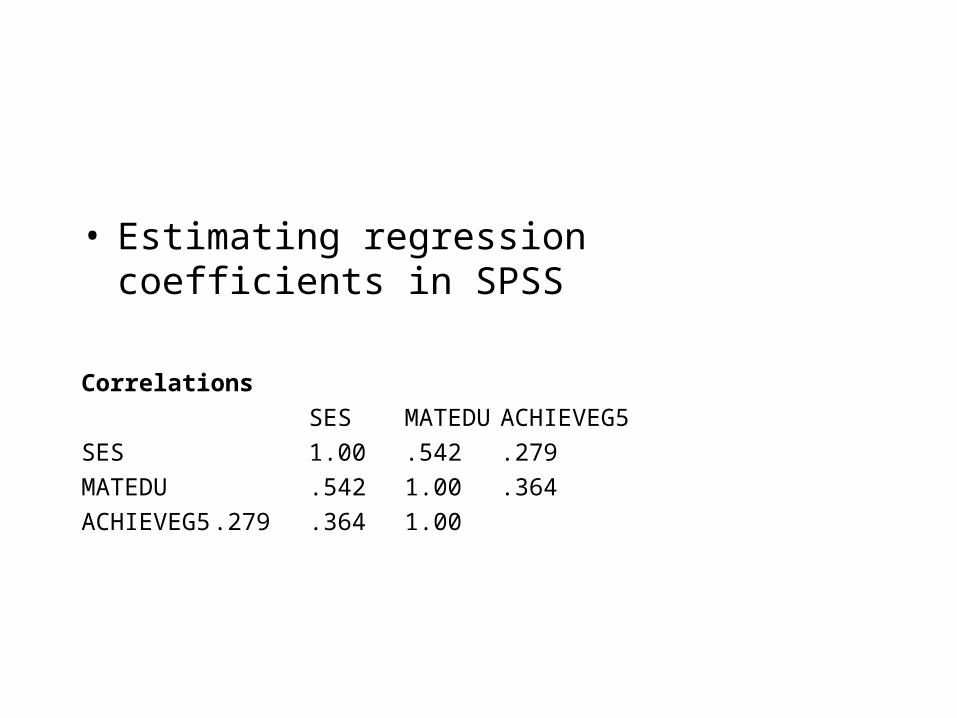
• Estimating regression coefficients in SPSS
Correlations
SES MATEDU ACHIEVEG5
SES 1.00 .542 .279
MATEDU .542 1.00 .364
ACHIEVEG5.279 .364 1.00


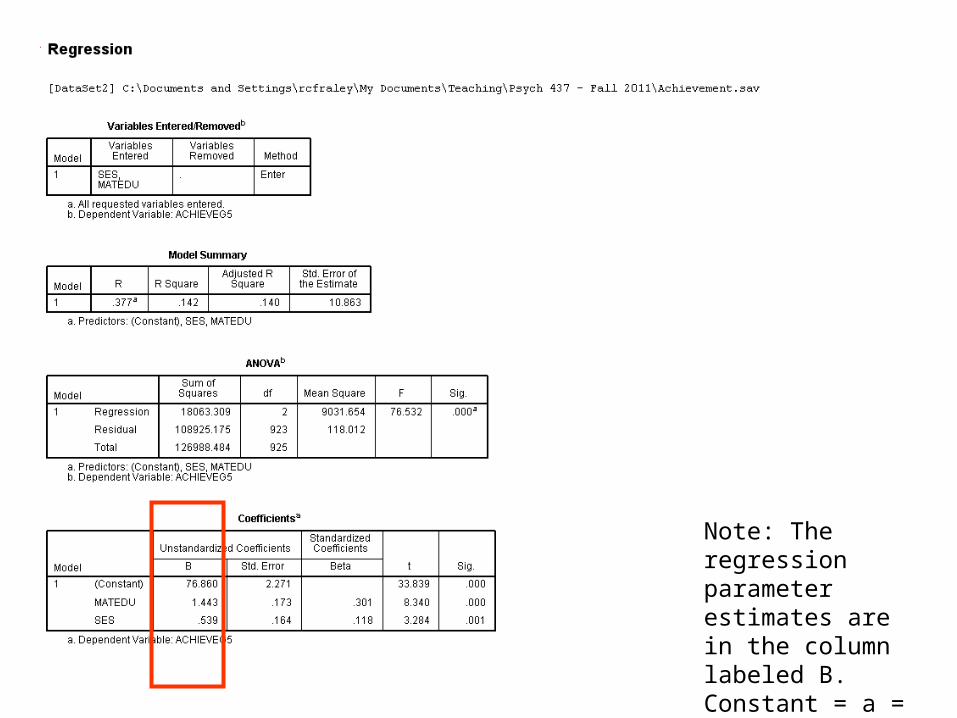
Note: The regression parameter estimates are in the column labeled B. Constant = a = intercept
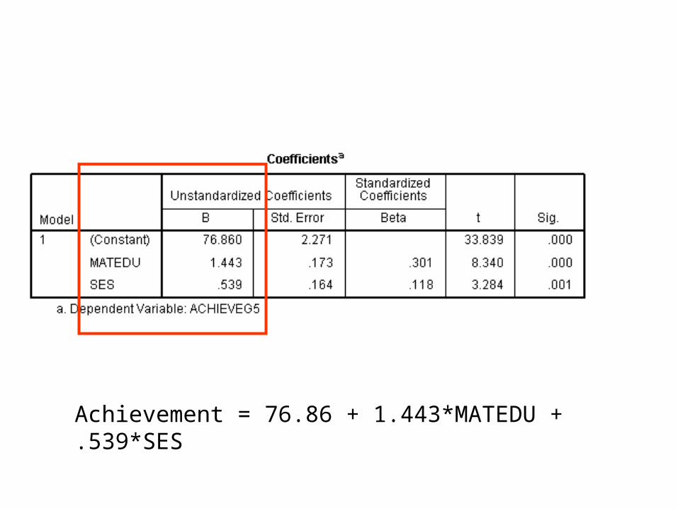
Achievement = 76.86 + 1.443*MATEDU + .539*SES
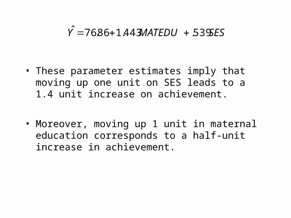
• These parameter estimates imply that moving up one unit on SES leads to a 1.4 unit increase on achievement.
• Moreover, moving up 1 unit in maternal education corresponds to a half-unit increase in achievement.
SESMATEDUY 539.443.186.76ˆ
• Does this mean that Maternal Education matters more than SES in predicting educational achievement?
• Not necessarily. As it stands, the two variables might be on very different metrics. (Perhaps MATEDU ranges from 0 to 20 and SES ranges from 0 to 4.) To evaluate their relative contributions to Y, one can standardize both variables or examine standardized regression coefficients.
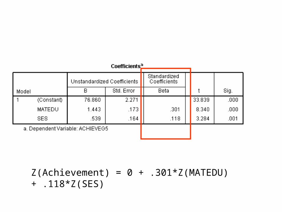
Z(Achievement) = 0 + .301*Z(MATEDU) + .118*Z(SES)
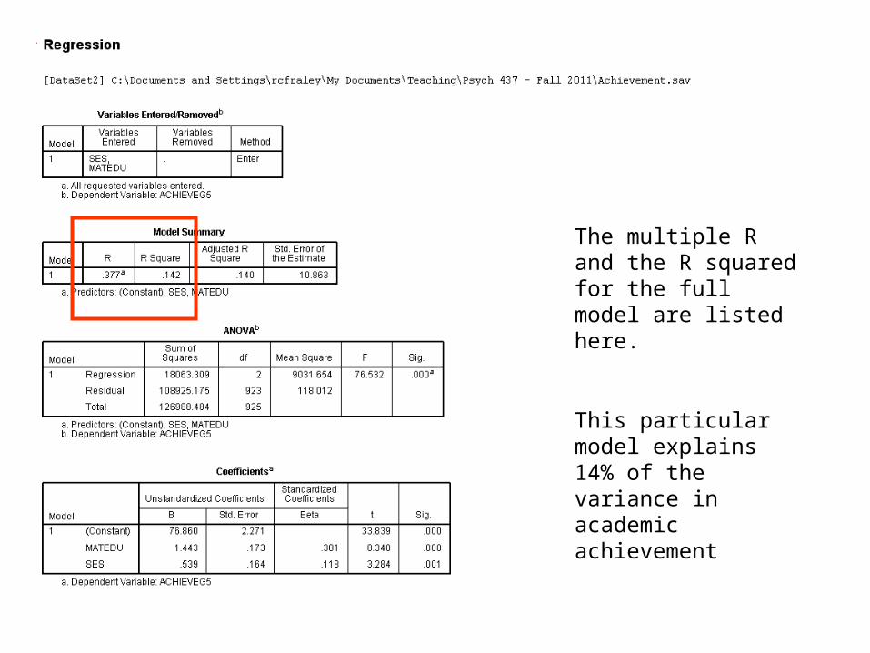
The multiple R and the R squared for the full model are listed here.
This particular model explains 14% of the variance in academic achievement
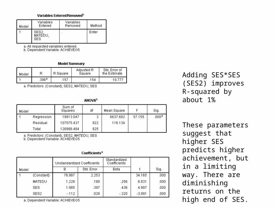
Adding SES*SES (SES2) improves R-squared by about 1%
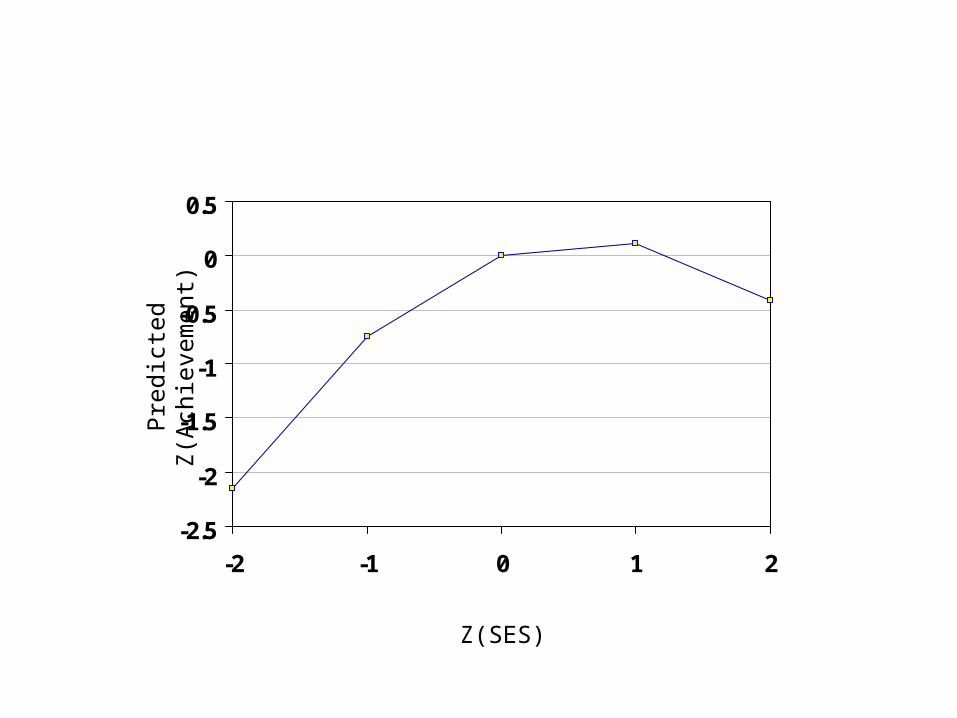
These parameters suggest that higher SES predicts higher achievement, but in a limiting way. There are diminishing returns on the high end of SES.
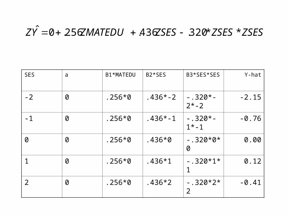
SES a B1*MATEDU B2*SES B3*SES*SES Y-hat
-2 0 .256*0 .436*-2 -.320*-2*-2 -2.15
-1 0 .256*0 .436*-1 -.320*-1*-1 -0.76
0 0 .256*0 .436*0 -.320*0*0 0.00
1 0 .256*0 .436*1 -.320*1*1 0.12
2 0 .256*0 .436*2 -.320*2*2 -0.41
ZSESZSESZSESZMATEDUYZ **320.436.256.0ˆ
-2.5
-2
-1.5
-1
-0.5
0
0.5
-2 -1 0 1 2
Z(SES)
Pred
icte
d Z
(Ach
ieve
men
t)