Baseline Control Systems in the Intelligent Building

NIST Technical Note 2178

Baseline Control Systems in the Intelligent Building Agents Laboratory

Amanda J. Pertzborn, Ph.D. Daniel A. Veronica, Ph.D., P.E.

This publication is available free of charge from: https://doi.org/10.6028/NIST.TN.2178

NIST Technical Note 2178

Baseline Control Systems in the Intelligent Building Agents Laboratory

Amanda J. Pertzborn, Ph.D. Building Energy and Environment Division

Engineering Laboratory

Daniel A. Veronica, Ph.D., P.E. Building Energy and Environment Division

Engineering Laboratory


September 2021

U.S. Department of Commerce Gina M. Raimondo, Secretary

National Institute of Standards and Technology

James K. Olthoff, Performing the Non-Exclusive Functions and Duties of the Under Secretary of Commerce for Standards and Technology & Director, National Institute of Standards and Technology

Certain commercial entities, equipment, or materials may be identified in this document in order to describe an experimental procedure or concept adequately.

Such identification is not intended to imply recommendation or endorsement by the National Institute of Standards and Technology, nor is it intended to imply that the entities, materials, or equipment are necessarily the best available for the purpose.

National Institute of Standards and Technology Technical Note 2178 Natl. Inst. Stand. Technol. Tech. Note 2178, 73 pages (September 2021)

CODEN: NTNOEF


i

This publication is available free of charge from: https://doi.org/10.6028/N

IST.TN.2178

Abstract The goal of the Embedded Intelligence in Buildings program at the National Institute of Standards and Technology (NIST) is to develop and deploy advances in measurement science that will improve building operations to achieve lower operating costs, increased energy efficiency, and improved occupant comfort, safety and security through the use of intelligent building systems. This program closely aligns with the overall NIST mission to promote U.S. innovation and competitiveness by anticipating and meeting the measurement science, standards, and technology needs of U.S. industry, and in this case, the U.S. building design, construction, and renovation industry. A principal asset to this program is the Intelligent Building Agents Laboratory (IBAL).

The IBAL provides the physical and computational infrastructure necessary to develop and test advanced agent–based optimization techniques to improve the energy and comfort performance of large buildings by focusing on control of heating, ventilation, and air-conditioning (HVAC) equipment. The goal of this document is to orient researchers to the baseline control systems in the IBAL and the general field of HVAC controls.

Key words building controls; HVAC; heating, ventilating, and air conditioning; intelligent agents; local control; PID; supervisory control.

ii


IST.TN.2178

Table of Contents

Introduction .................................................................................................................. 1

1.1. Purpose of the Intelligent Building Agents Laboratory ............................................. 1

1.2. Purpose of this Document .......................................................................................... 1

1.3. Intelligent Agents and their Benefits .......................................................................... 2

1.4. Technology of HVAC Control, in Real Buildings and in the IBAL .......................... 2

1.5. Hierarchy of HVAC Control, in Real Buildings and in the IBAL ............................. 3

1.6. Subjects of Local Loop Control, in Real Buildings and in the IBAL ........................ 3

1.6.1. Control Subjects Common to Real Buildings and to the IBAL .......................... 3

1.6.2. Control Subjects Unique to the IBAL ................................................................. 4

1.6.3. Overview of IBAL Systems ................................................................................ 4

Basic Science of Local Controls for HVAC ............................................................... 9

2.1. Local Loop Control of a Subject ................................................................................ 9

2.2. Tuning ...................................................................................................................... 11

Zone Controls in Real Buildings and in the IBAL .................................................. 14

3.1. Thermally Zoning a Building for a Controllable Indoor Environment .................... 14

3.2. Zone Loads ............................................................................................................... 14

3.2.1. Zone Cooling Loads .......................................................................................... 14

3.2.2. Zone Heating Loads .......................................................................................... 16

3.3. Zone Components and Processes ............................................................................. 16

3.3.1. Zone Components ............................................................................................. 17

3.3.2. A Psychrometric Chart ...................................................................................... 19

3.3.3. Zone Control on a Psychrometric Chart ........................................................... 21

3.4. Zone Simulation in the IBAL ................................................................................... 27

3.5. Zone Control in the IBAL ........................................................................................ 30

3.5.1. Volume Control ................................................................................................ 31

3.5.2. Reheat ............................................................................................................... 32

3.5.3. Airflow and Temperature Reset ........................................................................ 32

AHU Controller .......................................................................................................... 39

4.1. Air Dampers ............................................................................................................. 39

4.2. Supply Air Temperature ........................................................................................... 42

4.3. Supply Air Temperature Reset ................................................................................. 43

4.4. Fan Speed ................................................................................................................. 45

4.5. Static Pressure Reset ................................................................................................ 46

iii


IST.TN.2178

Hydronic System Controllers .................................................................................... 49

5.1. Chiller Controller ..................................................................................................... 49

5.2. Bridge Temperature Controller ................................................................................ 52

5.3. Supervisory Level Controllers Based on the Cooling Coil Valves .......................... 53

5.3.1. CHWST............................................................................................................. 55

5.3.2. Secondary Loop Differential Pressure Reset .................................................... 57

5.4. Thermal Storage Controller ...................................................................................... 59

Other Controllers in the IBAL ................................................................................. 61

6.1. Secondary Loop Temperature Setpoint .................................................................... 61

6.2. Water–side Economizer Operation .......................................................................... 61

6.3. Air–side Economizer Operation ............................................................................... 61

6.4. Primary Loop Flow Rate .......................................................................................... 61

6.5. Condensing Loop Flow Rate .................................................................................... 62

Further Reading ......................................................................................................... 63

References .............................................................................................................................. 64

iv


IST.TN.2178

List of Tables

Table 1. Tunable parameters in the PID controller. ............................................................... 12 Table 2. Current values of the tunable PI parameters ............................................................ 30 Table 3. Current values of the tunable PI parameters ............................................................ 30 Table 4. Current values of the tunable PI parameters ............................................................ 31 Table 5. Current values of the tunable PI parameters ............................................................ 32 Table 6. Variables in the flow and temperature reset controller. ........................................... 35 Table 7. Tunable variables in the flow and temperature reset controller. .............................. 35 Table 8. Current values of the tunable PI parameters ............................................................ 37 Table 9. Current values of the tunable PI parameters ............................................................ 38 Table 10. Current values of the tunable PI parameters for percent emulated outdoor air control. .................................................................................................................................... 40 Table 11. Variables in the percent emulated outdoor air flow controller. ............................. 40 Table 12. Current values of the tunable PI parameters .......................................................... 43 Table 13. Tunable variables in the supply air temperature reset controller. .......................... 44 Table 14. Current values of the tunable PI parameters .......................................................... 46 Table 15. Tunable variables in the static pressure reset controller. ....................................... 47 Table 16. Variables and parameters used in the control logic for staging chillers on and off.................................................................................................................................................. 50 Table 17. Current values of the tunable PI parameters .......................................................... 53 Table 18. Variables used to determine the CHWST or DP mode. ......................................... 55 Table 19. Variables in the CHWST controller. ...................................................................... 56 Table 20. Variables in the differential pressure reset controller in the secondary loop. ........ 58 Table 21. Current values of the tunable PI parameters for ..................................................... 59 Table 22. Current values of the tunable PI parameters for TS valve control. ........................ 60 Table 23. Further reading. ...................................................................................................... 63

v


IST.TN.2178

List of Figures

Fig. 1 Sketch of the key equipment in one of two AHU circuits in the air–side system. The other circuit is identical. ............................................................................................................ 5 Fig. 2. Sketch of the OAU. ....................................................................................................... 6 Fig. 3. Sketch of the condensing loop....................................................................................... 6 Fig. 4. Key elements of the primary loop. ................................................................................ 7 Fig. 5. Key elements of the secondary loop. ............................................................................. 8 Fig. 6 Example of a local control loop of an air temperature using a coil control valve. ......... 9 Fig. 7. Symbolic representation of the PI calculation. ............................................................ 11 Fig. 8 Possible temperature profiles under PI control. ........................................................... 13 Fig. 9 Generalized depiction of a zone with accompanying HVAC system. ......................... 17 Fig. 10 Psychrometric chart showing summer and winter design conditions. ....................... 20 Fig. 11. PI loop for the sensible load in the zone. .................................................................. 28 Fig. 12. PI loop for the latent load in the zone. ...................................................................... 29 Fig. 13. PI loop for the VAV damper position. ...................................................................... 31 Fig. 14. VAV reheat PI controller. ......................................................................................... 32 Fig. 15. Sketch of the airflow and temperature profiles for control. ...................................... 34 Fig. 16. Pseudocode for determining the operating mode in the VAV airflow and temperature reset controller. ....................................................................................................................... 35 Fig. 17. PI loop that calculates ∀𝑆𝑆𝑆𝑆 from the zone temperature and feeds to the VAV damper control signal. This loop is used in cooling mode or in heating mode if the reheat temperature is at its maximum value. ......................................................................................................... 36 Fig. 18. PI loop that calculates Td,SP from the zone temperature and feeds to the VAV heater control signal. .......................................................................................................................... 37 Fig. 19. PI loop that modulates the emulated outdoor air damper to achieve the percent emulated outdoor air setpoint, Peoa,SP. ..................................................................................... 39 Fig. 20. Pseudocode for determining the operation of the return air and exhaust dampers for percent SA control. ................................................................................................................. 41 Fig. 21. PI loop that modulates the cooling coil valve to bring the supply air temperature, Tsa, to the setpoint, Tsa,SP. ............................................................................................................... 42 Fig. 22. Pseudocode for determining the supply air temperature setpoint for the AHU. ....... 45 Fig. 23. PI loop that modulates the fan speed to bring the duct static pressure, Pstatic, to the static pressure setpoint, Pstatic,SP. .............................................................................................. 46 Fig. 24. Pseudocode describing the static pressure reset logic. .............................................. 48 Fig. 25. PI loop for the SL valve position............................................................................... 52 Fig. 26. Sketch of the coordinated operation of the secondary loop DP and CHWST controllers. .............................................................................................................................. 54 Fig. 27. Pseudocode for determining if CHWST or DP controller is primary. ...................... 54 Fig. 28. Pseudocode for calculating Tchwst. ............................................................................. 56 Fig. 29. Location of the pressure drop measurement in the SL. ............................................. 57 Fig. 30. Pseudocode for determining the differential pressure setpoint for the secondary loop pump. ...................................................................................................................................... 58 Fig. 31. PI loop for the SL pump speed. ................................................................................. 59 Fig. 32. PI loop for the TS valve position............................................................................... 60

1


IST.TN.2178

Introduction

The goal of the Embedded Intelligence in Buildings program at the National Institute of Standards and Technology (NIST) is to develop and deploy advances in measurement science that will improve building operations to achieve lower operating costs, increased energy efficiency, and improved occupant comfort, safety and security through the use of intelligent building systems. This program closely aligns with the overall NIST mission to promote U.S. innovation and competitiveness by anticipating and meeting the measurement science, standards, and technology needs of U.S. industry, and, in this case, the U.S. building design, construction, and renovation industry. A principal asset to this program is the Intelligent Building Agents Laboratory (IBAL).

1.1. Purpose of the Intelligent Building Agents Laboratory

Achieving a national goal of net zero energy buildings requires substantial reduction in the energy consumption of commercial building systems. Although significant progress has been made in the integration of building control systems through the development of standard communication protocols, such as BACnet and BACnet/IP, little progress has been made in making them “intelligent” about optimizing building system–level performance. The IBAL provides the physical and computational infrastructure necessary to develop and test advanced agent–based optimization techniques to improve the energy and comfort performance of large buildings.

The phrase “large buildings” refers specifically to buildings large enough to have a heating, ventilating, and air–conditioning (HVAC) system comprised of one or more chiller units, air–handling units, and air distribution or terminal units. Some large buildings might also be heated by the circulation of steam or hot water from a boiler plant. Such HVAC systems present optimization challenges at a level of complexity that requires research in a laboratory with the capabilities of the IBAL. The IBAL does not address buildings whose HVAC needs are met through self–contained, packaged equipment, a category ranging from private residences to small and mid–sized commercial or institutional structures, as seen in strip–malls. See Refs [1–3] for a thorough introduction to the IBAL design and capabilities.

1.2. Purpose of this Document

The IBAL is a piece of research infrastructure that bridges multiple scientific disciplines—HVAC and artificial intelligence to name two of them—bringing together people in the academic and industrial sectors who may have previously had little to no contact with each other. A likely scenario is that a post–doctoral researcher from the artificial intelligence academic community wants to apply a novel technique to a problem that the IBAL addresses but has no prior background in the HVAC process and control technologies typically encountered in the large buildings that the IBAL emulates. This document is primarily aimed at helping orient such a researcher to the IBAL control systems and the HVAC field of science that the IBAL serves.

The sections that follow discuss both the physics and technology found in large buildings, along with the physics and technology the IBAL employs to emulate the complexity of those buildings within the confines of the approximately 680 m3 (24,000 ft3) room it inhabits. The end goal is not measuring and improving the performance of a laboratory, but rather measuring and improving

2


IST.TN.2178

the performance of real buildings, so this document goes to some length to describe how real buildings work as a primer for understanding why control systems in the IBAL work as they do. But first, this introduction continues with further subsections on intelligent agents and the two–level control hierarchy into which they are implemented.

1.3. Intelligent Agents and their Benefits

An intelligent agent can take many forms, but the basic concept is that it acquires information about the state of the system (environment), makes an optimal or near–optimal control decision, and communicates that decision to another agent or to an actuator that executes the decision. The agent can represent a piece of HVAC equipment such as an air–handling unit (AHU) and learn how that AHU operates over time to produce an optimal or near–optimal operating point given the current or forecast system conditions. An HVAC system would contain multiple agents that communicate to make choreographed control decisions that lead to optimal or near–optimal operation of the overall system. In this way the decision–making process is distributed.

The optimal operation of one piece of equipment often conflicts with the optimal operation of another piece of equipment. For example, the AHU may have optimal performance when the chiller provides it with water at 1.7 °C (35 °F), but the chiller may have better performance producing water at 12.8 °C (55 °F). In one approach, at each timestep one agent determines how it would like to operate its equipment, calculates the cost of that operation, and communicates with the other agents to determine what the impact of that operation is on the other equipment in the system and the overall system cost. The agent can then decide if, given the overall impact on the system, it should change its setpoint as proposed. In the next timestep, a different agent leads this process. This is a round robin approach.

Kelly and Bushby [4] completed a feasibility study to determine if intelligent agent technology could lead to significant savings in HVAC energy consumption. They showed that, in a simulation of a single day of operation, the cost savings over a reference case without optimization was 21 %. Although the authors note that these savings are dependent on the details of the reference case, this proof–of–concept study was promising enough to justify the construction of a laboratory to test the concept using actual HVAC equipment. The IBAL is the culmination of that effort. The IBAL contains an air system able to emulate those typically found in commercial buildings and a hydronic system able to emulate a variety of designs typical of the chiller plant in a commercial building. The IBAL can represent a building with a modern, efficient HVAC system, or a building constrained by an older, more obsolescent design.

1.4. Technology of HVAC Control, in Real Buildings and in the IBAL

One way that buildings with HVAC systems of the complex, extensive sort that the IBAL emulates differ from smaller buildings with singular packaged equipment is in the control technology they require. While residential or light commercial packaged equipment can be fully controlled using a single, proprietary embedded microcontroller module, the extensive HVAC system of a larger building must have a control system of complementary extent, integrating the regulation of all the building’s many and dispersed HVAC components. Such a control system is often called a building automation system (BAS), although other terms for it, such as building energy management system (BEMS), are also used. The BAS is both hardware and software. It is

3


IST.TN.2178

the primary “embedding” when “embedded intelligence in buildings” is spoken of for large buildings.

The hardware elements of a BAS are principally temperature, pressure, flow, and other types of measurement instruments, microcontroller units, input and output interfaces, and actuators. The degree of functional integration of those elements, the physical centralization or distribution of those elements, and the means of data connectivity between those elements are all characteristics that vary widely among BAS installations, based on factors such as the age of a given installation and the state of technologies at that time.

The software elements of a BAS include a language (either text or graphically based) to program and store control logic for all the HVAC components the BAS regulates, along with a runtime element that executes the logic in real–time, and a user interface (UI) element that provides the building maintenance staff with real–time and event–driven interactivity, as well as access to historical trend data. The IBAL does not use a BAS for control. Instead, control logic is implemented in a graphical based software called LabVIEW.

1.5. Hierarchy of HVAC Control, in Real Buildings and in the IBAL

Control systems for HVAC can be thought of as having two hierarchical levels, local and supervisory. Supervisory control is the level that makes big picture decisions, such as which of two chillers to use to meet the current building load and what the setpoint temperature of the water from the chiller should be. Local control is used to control a single process or action based on the system conditions. For example, in a typical application a valve modulates to control a temperature to a setpoint calculated by the supervisory level. Numerous local control loops are used throughout the IBAL. The intelligent agent techniques described earlier are applied to the supervisory level while the local control uses traditional proportional–integral–derivative (PID) control.

1.6. Subjects of Local Loop Control, in Real Buildings and in the IBAL

Before discussing HVAC controls in depth, it is useful to identify the specific control subjects that will be the focus of this document, as well as the high–level details about the layout of the subjects within the IBAL.

1.6.1. Control Subjects Common to Real Buildings and to the IBAL

The HVAC system of a real building of the sort the IBAL can emulate will have one or more instances in each of the following categories as the subjects of local loop controllers:

• Air–side system:

o Variable air volume units (“VAV boxes”) serving individually controlled thermal zones

o Air handling units (AHU), which include dampers, coils, and fans o Exhaust fans

• Hydronic system (sometimes called the “water-side” system):

4


IST.TN.2178

o Chillers (typically only individual on/off control is made available to the interoperable BAS, with the chiller’s refrigeration process regulated by a packaged controller proprietary to the chiller vendor)

o Individually controlled pumps in both primary and secondary hydronic loops o Bridge piping between primary and secondary hydronic loops (control valving at

the bridge is optional) o Cooling tower, with controls for valve and fans (simulated in the IBAL via a

mixing valve and site chilled water) o Thermal (ice) storage tank (optional) o Waterside economizer (an optional heat exchanger between the primary loop and

cooling tower)

Some real buildings have HVAC components the IBAL does not have and cannot simulate, such as dual–duct AHU and dual–duct VAV boxes, fan–powered boxes, multizone units, fan–coil units, return fans, boilers, and heat–recovery or desiccant wheels. The list of local loop controller subjects for those buildings would be at least partly different from that above. The type of air–side system defined by the list above, and the type implemented in the IBAL, is known in [5] as “single–duct VAV with terminal reheat”. The hydronic system listed is a type generally known as primary–secondary with multiple stageable chillers and thermal storage.

1.6.2. Control Subjects Unique to the IBAL

Because of the obvious constraints of being a laboratory housed in a NIST building, the IBAL cannot present its air–side and hydronic systems with full–sized, occupied, equipped spaces to heat or cool. Further, a controllable source of “weather” must be available to allow for repeatable experiments. Those factors add the following local loop control subjects to the above list; subjects in the IBAL that are not found in any real building:

• Air–side system:

o Zone simulators, equipped and programmed to present sensible and latent loads to the air–side

o Outdoor air unit (OAU), equipped and programmed to present repeatable outdoor air conditions to the air–side

• Hydronic system:

o Heat exchanger to support IBAL experiments loading the hydronic system (e.g., chillers and thermal storage) without operating the air–side system

o Mixing valve and site chilled water to simulate the heat–sink effect of a cooling tower and the wet–bulb condition it is in

1.6.3. Overview of IBAL Systems

The layout of the key air–side and hydronic system equipment in the IBAL is presented in this section. Figure 1 is a sketch of one of the two AHUs serving multiple zones in the air–side, composed of an AHU, two VAV boxes (aka terminal units), and two zones. The hydronic system connects to the air–side system via the cooling coils in the AHUs. This figure highlights Tz, the

5


IST.TN.2178

zone temperature (which is different for each zone). The air–side and hydronic systems work together to maintain Tz at setpoint Tz,SP, which is typically around 22.2 °C (72 °F). Zone humidity is not currently controlled in the IBAL.

Each zone contains an electric heater that emulates sensible zone cooling loads, such as those generated by computer equipment and lights, and a steam spray humidifier that emulates latent zone loads (i.e., the moisture given off by people or from outside air). The AHUs contain an electric heater that preheats the inlet air in cold weather to prevent damage to the cooling coil, a cooling coil that cools and/or dehumidifies the air, and a supply air fan that moves air through the system. Each VAV contains a damper that modulates airflow and an electric heater that reheats the air based on the needs of the individual zone. Background on the operation of these systems is presented in Sec. 3.

Fig. 1 Sketch of the key equipment in one of two AHU circuits in the air–side system. The other circuit is identical.

Figure 2 is a sketch of the OAU, also referred to as the weather emulator. It takes the real outdoor air, to the left in the figure, and conditions it to generate repeatable climate conditions at the inlet to the AHUs. The cooling coil, electric heater, and steam spray humidifier operate in concert to cool, dehumidify, heat (or reheat), and humidify the outdoor air. The operation of the OAU will be documented in a future NIST technical note.

Heater Cooling Coil

Fan

Heater

Tz

Steam Spray Humidifier

AHU VAV Zone

Damper

6


IST.TN.2178

Fig. 2. Sketch of the OAU.

The hydronic system uses a primary–secondary configuration; the plant equipment is in the primary loop and the loads (via the cooling coils and a heat exchanger) are in the secondary loop. Figure 3 shows the condensing loop, with the key components labeled. This loop provides cooling water to the condensers in the chillers and to the water–side economizer (WSE), emulating a cooling tower in a real building. The cold water for the loop is supplied by the NIST site chilled water, which is approximately 5.6 °C (42 °F). The temperature of this water is tempered by use of the mixing valve, V3, which controls the amount of warmer return water from the condensers in the chillers or the WSE that mixes with the cold site chilled water. The heat exchanger labeled “HX2” is connected to the site hot water (71 °C or 160 °F) and can be used to mitigate temperature fluctuations in the condensing loop that occur when a chiller starts up or shuts down. This process allows us to supply water to the chillers and WSE at a temperature similar to that supplied by a real cooling tower, ranging from 24 °C to 29.4 °C (75 °F to 85 °F).

Fig. 3. Sketch of the condensing loop.

Heater Cooling Coil

Steam Spray Humidifier

Fan

To AHUs Real Outdoor Air

Site Chilled Water

Chiller2 Chiller1 Water–side Economizer

V3

HX2

Site Hot Water

7


IST.TN.2178

Figure 4 shows the primary loop, including how it connects to the condensing loop via the chillers and the WSE, which is a plate heat exchanger. The chillers, WSE, or ice–on–coil thermal storage tank are designed to meet building cooling loads. This equipment is referred to collectively as the chiller plant.

Fig. 4. Key elements of the primary loop.

Figure 5 shows the secondary loop and how it connects the hydronic and air–side systems. The IBAL uses a 30 % propylene glycol (PG) brine in the primary and secondary loops. Simulated building loads are generated by any combination of the heat exchanger, HX1, and the cooling coils in the two AHUs. The primary and secondary loops are connected by a bridge. This bridge can serve two purposes: 1) to hydraulically separate the loops at the pipe labeled “S” so that each loop can have a different flow rate; 2) to modulate the temperature in the secondary loop by use of a mixing valve in the same way the mixing valve in the condensing loop controls that temperature. When the system includes ice thermal storage, there are times when the primary loop must operate below the freezing point of pure water to build ice in the tank. If the secondary loop operates at the same time to meet building loads, the temperature of the liquid will be far colder than what is typically required, so the mixing valve will modulate to ensure that the temperature of the liquid in the secondary loop matches the need of the load. When that is not the case, the second purpose is often not needed, so the mixing valve and the pipe labeled “P” are not always present in a real building. Having the complete bridge allows the IBAL to emulate either situation.

Chiller2 Chiller1 Water–side Economizer

Cooling water

From Secondary Loop

To Secondary Loop

Thermal Storage

Condensing Loop (Cooling tower)

Primary Loop

8


IST.TN.2178

Fig. 5. Key elements of the secondary loop.

Cooling Coil: AHU1

Cooling Coil: AHU2 HX1

Hot Water

PG

Air

Secondary Loop

To/From Primary Loop

Bridge

P S

9


IST.TN.2178

Basic Science of Local Controls for HVAC

2.1. Local Loop Control of a Subject

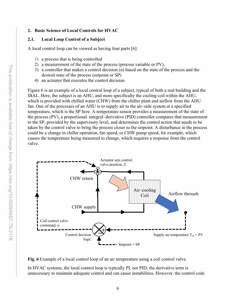
A local control loop can be viewed as having four parts [6]:

1) a process that is being controlled 2) a measurement of the state of the process (process variable or PV), 3) a controller that makes a control decision (u) based on the state of the process and the

desired state of the process (setpoint or SP) 4) an actuator that executes the control decision

Figure 6 is an example of a local control loop of a subject, typical of both a real building and the IBAL. Here, the subject is an AHU, and more specifically the cooling coil within the AHU, which is provided with chilled water (CHW) from the chiller plant and airflow from the AHU fan. One of the processes of an AHU is to supply air to the air–side system at a specified temperature, which is the SP here. A temperature sensor provides a measurement of the state of the process (PV), a proportional–integral–derivative (PID) controller compares that measurement to the SP, provided by the supervisory level, and determines the control action that needs to be taken by the control valve to bring the process closer to the setpoint. A disturbance in the process could be a change in chiller operation, fan speed, or CHW pump speed, for example, which causes the temperature being measured to change, which requires a response from the control valve.

Fig. 6 Example of a local control loop of an air temperature using a coil control valve.

In HVAC systems, the local control loop is typically PI, not PID; the derivative term is unnecessary to maintain adequate control and can cause instabilities. However, the control code

Air–cooling

Coil

+ – Setpoint = SP

Control decision logic

Supply air temperature Tsa = PV

Actuator sets control valve position, Z

Airflow through

Coil control valve command, u

CHW supply

CHW return

10


IST.TN.2178

in the IBAL includes the derivative term in case it is needed. The basic equation for the PID algorithm is given in Eq. (1), where P is the proportional term, I is the integral term, and D is the derivative term; uraw is the initial calculated value of the control signal u.

𝑢𝑢𝑟𝑟𝑟𝑟𝑟𝑟 = 𝑆𝑆 + 𝐼𝐼 + 𝐷𝐷 (1)

Eqs. (2)–(4) define the P, I, and D terms. The proportional, integral, and derivative gains are Kp, KI, and Kd, respectively. Each gain is multiplied by a form of the error and is tuned to obtain the desired control response. The P term scales the control signal in proportion to the error (Eq. (5)). If Kp is large, the controller will respond to a disturbance more quickly, but if it is too large, the PV can overshoot the SP, then undershoot the SP, and continue oscillating. If Kp is small, the controller will be stable, but sluggish. Even when Kp is tuned such that P is stable, it can reach a steady state where the error term is constant, and the PV is at a constant offset from the SP.

𝑆𝑆 = 𝑒𝑒 𝐾𝐾𝑝𝑝 (2)

The I term is used to eliminate this offset. KI is multiplied by the sum of the error (Eq. (6)), so even if the error is constant, this constant error will accumulate, causing I to increase (or decrease, depending on the direction of the error), which will bring the PV closer to SP. The D term is obtained by multiplying the coefficient Kd by the rate of the error (Eq. (7)); it can be used to anticipate changes in the system. It is, however, very sensitive to noise and can de–stabilize the system.

𝐼𝐼 = 𝑒𝑒𝐼𝐼 𝐾𝐾𝐼𝐼 (3)

𝐷𝐷 = 𝑒𝑒𝑟𝑟𝑟𝑟𝑟𝑟𝑟𝑟 𝐾𝐾𝑑𝑑 (4)

The error, e, is defined in Eq. (5). In its most basic form, it is just the difference between PV and SP, but in the IBAL it is scaled by the maximum (SPHigh) and minimum (SPLow) values of the SP. By scaling the error, the gains in different parts of the lab are on a similar scale, which can simplify the tuning procedure. The integral error, eI (Eq. (6)), is the sum of the errors multiplied by the timestep dt. An anti–windup technique is used to prevent eI from becoming too large; if the control signal is near its maximum or minimum, the error does not accumulate until the sign of the error is the opposite of the sign of the accumulated error. This latter feature is required to prevent the controller from getting “stuck” at one of the limits. The error rate, erate (Eq. (7)), is the current error minus the previous error, divided by dt. In the IBAL dt = 10 s.

𝑒𝑒 = 𝑆𝑆𝑃𝑃 − 𝑆𝑆𝑆𝑆

𝑆𝑆𝑆𝑆𝐻𝐻𝐻𝐻𝐻𝐻ℎ − 𝑆𝑆𝑆𝑆𝐿𝐿𝐿𝐿𝑟𝑟 (5)

𝑒𝑒𝐼𝐼 = �𝑒𝑒𝑑𝑑𝑑𝑑 (6)

𝑒𝑒𝑟𝑟𝑟𝑟𝑟𝑟𝑟𝑟 =𝑒𝑒 − 𝑒𝑒𝑝𝑝𝑟𝑟𝑟𝑟𝑝𝑝

𝑑𝑑𝑑𝑑 (7)

The initial calculation of the control signal, shown in Eq. (1), is adjusted as shown in Eq. (8) to generate cbias, which is limited to a range of 0 to 1. The term A is action and has a value of –1 if the actuator is reverse acting and +1 if the actuator is direct acting. For example, if the goal of a

11


IST.TN.2178

process is to decrease temperature and the temperature decreases when the valve opens (u increases), it is reverse acting; if the temperature decreases when the valve closes (u decreases), it is direct acting. The term uBias is a bias term that provides coarse control of the system. If it is known that the typical position of the actuator is, for example, in the middle of its range, then setting uBias to a value of 0.5 can bring the control signal near the right control action and the remaining terms fine tune the control.

𝑐𝑐𝑏𝑏𝐻𝐻𝑟𝑟𝑏𝑏 = 𝑢𝑢𝐵𝐵𝐻𝐻𝑟𝑟𝑏𝑏 − 𝐴𝐴 𝑢𝑢𝑟𝑟𝑟𝑟𝑟𝑟, 𝑐𝑐𝑏𝑏𝐻𝐻𝑟𝑟𝑏𝑏 = [0,1] (8)

The final step is to convert cbias to engineering units. The control signal for a valve, for example, is often between 2 and 10 V, not 0 and 1, so the control signal is scaled as shown in Eq. (11), using the slope and intercept calculated in Eqs. (9) and (10). EUHigh and EULow are the high and low limits on the control signal (e.g. 10 V, 2 V), respectively; cbias,max and cbias,min are the limits on cbias, 1 and 0, respectively.

𝑠𝑠𝑠𝑠𝑜𝑜𝑝𝑝𝑒𝑒 =𝐸𝐸𝐸𝐸𝐻𝐻𝐻𝐻𝐻𝐻ℎ − 𝐸𝐸𝐸𝐸𝐿𝐿𝐿𝐿𝑟𝑟

𝑐𝑐𝑏𝑏𝐻𝐻𝑟𝑟𝑏𝑏,𝑚𝑚𝑟𝑟𝑚𝑚 − 𝑐𝑐𝑏𝑏𝐻𝐻𝑟𝑟𝑏𝑏,𝑚𝑚𝐻𝐻𝑚𝑚= 𝐸𝐸𝐸𝐸𝐻𝐻𝐻𝐻𝐻𝐻ℎ − 𝐸𝐸𝐸𝐸𝐿𝐿𝐿𝐿𝑟𝑟 (9)

𝑖𝑖𝑖𝑖𝑑𝑑𝑒𝑒𝑖𝑖𝑐𝑐𝑒𝑒𝑝𝑝𝑑𝑑 = 𝐸𝐸𝐸𝐸𝐻𝐻𝐻𝐻𝐻𝐻ℎ − 𝑠𝑠𝑠𝑠𝑜𝑜𝑝𝑝𝑒𝑒 𝑐𝑐𝑏𝑏𝐻𝐻𝑟𝑟𝑏𝑏,𝑚𝑚𝑟𝑟𝑚𝑚 = 𝐸𝐸𝐸𝐸𝐻𝐻𝐻𝐻𝐻𝐻ℎ − 𝑠𝑠𝑠𝑠𝑜𝑜𝑝𝑝𝑒𝑒 (10)

𝑢𝑢𝑏𝑏𝑠𝑠𝑟𝑟𝑠𝑠𝑟𝑟𝑑𝑑 = 𝑐𝑐𝑏𝑏𝐻𝐻𝑟𝑟𝑏𝑏 𝑠𝑠𝑠𝑠𝑜𝑜𝑝𝑝𝑒𝑒 + 𝑖𝑖𝑖𝑖𝑑𝑑𝑒𝑒𝑖𝑖𝑐𝑐𝑒𝑒𝑝𝑝𝑑𝑑 (11)

The PI calculation is represented in conventional symbols as shown in Fig. 7. The variable s is the Laplace transform and 1/s is integration. This convention is used throughout this document.

Fig. 7. Symbolic representation of the PI calculation.

2.2. Tuning

The PID gains are free parameters that are determined for each individual control loop. The process of determining these values is called tuning. Although in some cases the values can be estimated through theory and modeling (see [7], for example), in the IBAL we tune the loop while the system is running using the following approach [8]:

1) set KI = 0 and Kd = 0; 2) increase Kp until the control signal oscillates; 3) decrease Kp until the oscillations stop; 4) slowly increase KI until the PV is approximately at SP. Note: the integral error may need

to be reset during this step; 5) make a step change to the SP and see if the system stabilizes; adjust as needed.

PV

Kp

1𝑠𝑠

KI

+ – SP u

12


IST.TN.2178

Although oscillations are most associated with the P term, they can also be caused by an I term that is too large. PI controllers may also need to be re–tuned when additional controllers are added to the system or modified. The PID parameters that are set for loops in the IBAL are shown in Table 1.

Table 1. Tunable parameters in the PID controller. Name Description Kp Proportional gain KI Integral gain Kd Derivative gain SPHigh Upper bound on the SP SPLow Lower bound on the SP uBias Bias term A Action EUHigh Upper bound on the engineering unit

of the actuator EULow Lower bound on the engineering unit

of the actuator

Figure 8 shows four temperature profiles that can be encountered during tuning. The horizontal line is the setpoint temperature. One profile shows a steady oscillation, which is generally an indicator that Kp is too high – the system is too responsive to the error. There are also two cases of overshoot: 1) the PV overshoots the SP, oscillates around the SP a couple of times, and slowly settles to the SP; 2) the PV overshoots the SP and then slowly settles to the SP. Both situations are caused by Kp being too high, but not so high that the system will never stabilize. The fourth profile shows the temperature increase to the SP without over– or under–shooting. Of all the profiles in this figure, this is the “best” case because it reaches the SP in the least time. However, depending on the situation, it may take too long to reach SP in this scenario. In such a situation it may be better to increase the gain to overshoot the SP, but then stabilize to the SP quickly after the overshoot.

13


IST.TN.2178

Fig. 8 Possible temperature profiles under PI control. Time

PVOscillation

Overshoot

No over- or under-shoot

SP

14


IST.TN.2178

Zone Controls in Real Buildings and in the IBAL

Referring back to Sec. 1.6 and its list of local loop control subjects, the first subjects in the list are in the air–side system and they serve the building’s “individually–controlled thermal zones”. It fits with the physics of HVAC for the discussion of subjects and their controllers to begin at the thermal zones. The purpose of a building’s HVAC system is to provide a satisfactory indoor environment for people and the work they do, and the people and their work are all in thermal zones. So, zones are the endpoints of the whole HVAC system. All the components of the system are essentially participants in a sort of energy “bucket brigade”, passing energy either from zones to a sink (typically, the outdoors), or from a source to zones, with the direction and degree being decided by zone controllers.

3.1. Thermally Zoning a Building for a Controllable Indoor Environment

One of the first steps when designing the HVAC system for a particular building is laying out its thermal zones. While the architect divides the floor plan into rooms to achieve functional or aesthetic goals, the HVAC engineer divides the same plan into zones to foster controllability throughout the indoor environment while keeping the installed cost of the HVAC system within the project’s budget. The correspondence of zones to rooms is not necessarily one–to–one. A single, expansively open room intended as an office cubicle area, especially one bounded on multiple sides by exterior walls and windows of the building, might contain several zones. Conversely, multiple small interior rooms might be grouped into a single zone, especially if the installed cost has priority. Zoning divides the indoor environment into the distinct domains of individual HVAC controllers.

Proper zoning at the time the HVAC system is designed is a critical part of controllability once the building is in use. “Exterior zones”, those bounded by the building’s envelope (i.e., exterior walls, floor, ceiling or roof, and windows) should be separately controllable from “interior zones”, those which are bounded only by other zones. A clear example of that is in winter when interior zones of a large building may still require cooling despite the exterior zones needing heating, because interior zones have no boundary on the weather outside. In some situations that can happen whether or not there are partition walls between the zones. In summer, a large, open room could see the reverse effect. A cubicle area by an exterior wall with large, minimally–shaded glass facing the solar arc will need significantly more cooling than an area far inside, so it is “more controllable” to not have both areas in the same zone, regardless of the fact they are in the same room.

3.2. Zone Loads

In the HVAC industry, a “load” is a power quantity, a rate of energy transfer over a unit of time expressible in, for example, Watts, BTU/hour, or (for certain equipment types) “tons” (of refrigeration power). A building’s HVAC system must regulate its capacities in real–time to match the zone loads to fulfill its purpose of maintaining satisfactory steady–state conditions in the zones.

3.2.1. Zone Cooling Loads

The term “cooling load” means any influence tending to make a zone warmer or more humid, energy additions that the HVAC system must counteract with matching amounts of energy

15


IST.TN.2178

removal to keep the zone at a satisfactory steady–state condition. The part of that energy removal addressing warming is termed “sensible”, the part addressing humidity is termed “latent”. Zone cooling loads will be regarded here as potentially coming from five distinct sources:

1) people in the zone (sensible and latent) 2) equipment or appliances in the zone (sensible mostly, some equipment also latent) 3) lighting in the zone (sensible) 4) from outside the zone through the building envelope, including windows (sensible and

latent) 5) carried in ventilation air (i.e., outside air) required in the zone (sensible and latent)

The above says “potentially” coming into the zone because zone characteristics vary widely, and not all zones have all the above load sources, whether that means all the time or just some of the time. An equivalent parlance for cooling loads is to call them “heat gains”.

Just for an appreciation of the magnitudes involved, each person releases on average 100 to 528 W of total (sensible and latent) load to the zone, depending on activity level [9]. People sitting in an auditorium would be at the bottom of that range, while those active in a gymnasium would be at the top. So, a fully–attended function in the 750–seat NIST Red Auditorium would present a cooling load of about 75 kW just from the people, as would a large gym with 150 participants. About 40 % to 65 % of total people load is latent, through skin evaporation and breathing, depending similarly on activity level [10]. That latent range translates as 60 to 500 grams (2 to 17 fl. oz.) of water released as vapor each hour from each person. When the building’s HVAC system is designed, “design values” are defined for: 1) the number of people in the zones (which also sets the design ventilation requirement); 2) the equipment and lighting wattage per area of the zones; and 3) the outdoor conditions (summer and winter) that drive energy in, or draw it out, through the building envelope. Those design values are used in calculations that are the basis for selecting the sizes (capacities) of all the HVAC components in the system, including VAV boxes, AHUs, and chillers. The energy removal requirement for the whole building is estimated at the summer design condition and expressed on a per area basis averaged across all its conditioned floor area as a metric of overall system efficiency. Anecdotally, that metric has been seen to range from 54 W/m2 (5 W/ft2) in more efficient or in lightly (thermally) loaded buildings to 194 W/m2 (18 W/ft2) in less efficient or heavily loaded buildings. Taking the 124 W/m2 (11.5 W/ft2) middle value of that range, a hypothetical 37 m2 (400 ft2) zone in such a building would need 4.6 kW of energy removal.

Design values for weather do not correspond to any actual, individually recorded days, but are instead averages of outdoor conditions posing envelope and ventilation loads worse than a very high percentage (commonly, 97 or 99 %) of hourly weather readings recorded near the building’s location (often, a nearby airport) over many (typically 25) years [9]. In other words, at least 97 % of the time the cooling load in the hypothetical zone discussed above will be less than its 4.6 kW design value, and very often it will be far less. Despite that, the zone’s HVAC components, its VAV box for example, are sized to remove the design value cooling load. That explains why the entire HVAC system, starting with its zones, needs local loop controllers. To cover the extreme conditions of the design values, the system and its components must have far more capacity than what is needed most of the time.

16


IST.TN.2178

In actual practice, the individual design values for the five zone cooling loads listed above are not simply summed at their maximums to calculate capacities for (i.e., “sizing”, “selecting”) HVAC system components. That represents a circumstance too unlikely to be a realistic sizing basis because each of the loads is considered at maximum at the same time. A more realistic sizing basis scales the individual contributions from cooling load sources by “load factors” or “duty factors” so the total cooling load is markedly less than the coincidental sum of maximums from the individual sources. The factors, and the judgements made to apply them, add essential measures of practice and art to the imperfect science behind sizing HVAC components. This is important in regard to controls because local control loops of the traditional PID type typically have trouble regulating oversized HVAC components.

The rational basis for sizing a particular component is typically the need to meet a worst–case load, but that load rarely occurs in reality. Far more often the component will operate at much lower “partial–load” or “turn down” capacities rather than at “full–load” maximum. Under those conditions, some components will exhibit nonlinear behavior. Since effective tuning of a PID controller relies upon its component having a satisfactory degree of linearity across the operating range, the practical outcome of excessive nonlinearity is that control becomes inconsistent over the full range of operation. As a result, the controller has to be tuned to a narrower range of operation. Sometimes the better design is to down–size the component, sacrificing performance at the full–load operating point in the interests of controllability over a wider range of operating conditions. Any trade–off between controllability and full–load operation is something the design engineer considers for a specific application. Valves and dampers, whose many types are notably diverse in the degree of linearity they offer, also require particular attention for this reason. 3.2.2. Zone Heating Loads

The term “heating load” means any influence tending to make a zone cooler, an energy loss that the HVAC system must counteract with matching amounts of energy addition to keep the zone at satisfactory steady–state conditions. Here, heating load is always sensible; that is, always based upon dry–bulb temperature. Also, heating load will be regarded exclusively as heat lost from a zone through the building envelope to the outdoors. The problem of insufficient humidity, which can arise when a zone receives heat in winter, is addressed separately as a “humidification load”. Thus, it is equivalent to refer to heating loads as “heat losses”.

3.3. Zone Components and Processes

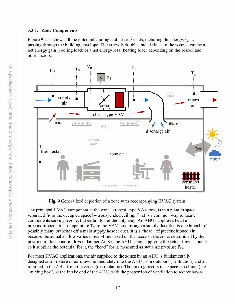
Figure 9 shows (in gray) a generalized depiction of a zone in a real building, along with (in black) the HVAC components employed to serve the zone in a single–duct VAV terminal reheat system. Dots to dashed lines show locations where quantities (temperatures, pressures, flows, etc.) that are relevant to discussing zone processes could be measured, but not all those quantities are necessarily actually measured and used by the zone controller. Instead, the number of quantities actually measured and used is a matter of matching controller sophistication to the challenges of the problem and the cost constraints on how those challenges are addressed. Further along in this section, we will show that controllers addressing the same problem have differing levels of sophistication, and the most sophisticated design is not necessarily the best for every situation. But first, a zone will be described from two perspectives, component and process.

17


IST.TN.2178

3.3.1. Zone Components

Figure 9 also shows all the potential cooling and heating loads, including the energy, Qenv, passing through the building envelope. The arrow is double–ended since, to the zone, it can be a net energy gain (cooling load) or a net energy loss (heating load) depending on the season and other factors.

Fig. 9 Generalized depiction of a zone with accompanying HVAC system.

The principal HVAC component at the zone, a reheat–type VAV box, is in a plenum space separated from the occupied space by a suspended ceiling. That is a common way to locate components serving a zone, but certainly not the only way. An AHU supplies a head of preconditioned air at temperature Tsa to the VAV box through a supply duct that is one branch of possibly many branches off a main supply header duct. It is a “head” of preconditioned air because the actual airflow varies in real–time based on the needs of the zone, determined by the position of the actuator–driven damper Zd. So, the AHU is not supplying the actual flow as much as it supplies the potential for it, the “head” for it, measured as static air pressure Psa.

For most HVAC applications, the air supplied to the zones by an AHU is fundamentally designed as a mixture of air drawn immediately into the AHU from outdoors (ventilation) and air returned to the AHU from the zones (recirculation). The mixing occurs in a space or cabinet (the “mixing box”) at the intake end of the AHU, with the proportion of ventilation to recirculation

R/H

supply air

discharge air

reheat–type VAV

zone air

return air damper

A

Tsa ∀̇𝑟𝑟 Tda Tra

Tz

Psa

perimeter heater

thermostat

lighting

occupants and equipment

plenum space

occupied space

diffuser grille

Zd

18


IST.TN.2178

principally set by the positions of dampers. Those dampers are under automatic control (see Sec. 4.1). Recirculation of already–conditioned air contributes to system efficiency, so ductwork providing a recirculation path is typically installed except in specific applications, such as some medical, laboratory, or industrial facilities. Having a recirculation path available, though, does not mean it should always be used. The “economizer” mode of AHU control reduces or completely forgoes mechanical cooling of recirculated air in favor of supplying zones with a larger proportion of outdoor air (even as high as 100 %) when the weather is sufficiently cool and dry. Air then leaves zones by the usual return paths, but a larger fraction is released back outside by the AHU as “exhaust” instead of being recirculated.

The object here is to regulate the state of what is shown as “zone air”, that is, the air around the occupants and their equipment. Depending upon the needs of the application—whether the zone is, for example, an office, a laboratory, or an isolation room in a hospital—that controlled “state” might mean not only temperature, but moisture level (humidity) or static air pressure as well. Cooling load is removed from the zone by the steady mixing into the zone of VAV box discharge air, which is cooler than the zone air. The careful placement of diffusers that discharge cool air to the occupied space and grilles that allow (commonly by a fan at the AHU) “return air” to be drawn from the occupied space ensure thorough mixing of the air. In warming up what had been the discharge air, this mixing sustains the path by which energy is removed from the zone; the return air has “picked up” the zone’s cooling load. Heating load, it might seem, could be “dropped off” by mixing in warmed air through the use of the VAV box’s reheat coil, but later it will be shown what purposes the reheat coil serves, and handling the heating load is not one of them. Instead, heating load—and again, typically only exterior zones need this—is handled by heating apparatus (radiators, baseboard units, etc.) located along the zone’s exterior walls (its “perimeter”), most commonly under windows.

Zone air temperature, Tz, is measured by a thermostat, which compares its measurement to the desired (setpoint) zone air temperature Tz,SP. In a single–duct VAV terminal reheat system, the temperature of air supplied to the VAV box, Tsa, is always lower than Tz. In fact, it is common that the system design expects it to be significantly lower, as in 6.7 to 8.3 °C (12 to 15 °F) lower. One reason for that is so the VAV box in the building with the design (i.e., worst–case) zone sensible cooling load will be able to meet that load while keeping the resulting airflow within its rated capacity. Another reason is that picking up the latent part of the cooling load requires the discharge air to be not just cooler, but drier (not by relative humidity, but by absolute moisture content) than the zone air.

There are various ways to pick up the latent load, but a very common approach, and the one taken as default in the IBAL, is to chill the water supplied to the AHU cooling coil enough to condense an equivalent amount of moisture out of the supply air. That is, a theoretical state property known as the coil’s apparatus dew point (ADP) is kept low enough that air leaving the AHU is sufficiently dry by absolute measure.

It is worth noting at this point that we have just seen our first example of the interrelatedness of the various processes happening in a HVAC system. Raising the temperature of the chilled water supplied to the AHU cooling coil can adversely affect the ability of zone controllers to regulate zone conditions. Not all the interrelations are immediately apparent. And, when control of a process goes wrong, the fault might not always be a problem in the local control loop, but rather

19


IST.TN.2178

a problem in what has happened to a related quantity not found in the local loop at all. An intelligent agent methodology acting in such a domain must account for all the consequences of its actions. Those consequences can be understood by analyzing the HVAC system as a network of individual, interacting processes. Under a single–duct VAV terminal reheat design, the processes removing energy from the zones are air–side processes. The accepted way of understanding air–side processes is to plot and analyze them on a psychrometric chart.

3.3.2. A Psychrometric Chart

The psychrometric chart in Fig. 10 shows two separate diagrams of HVAC system processes. One diagram is based upon outdoor conditions at summer design values, expressed by the point labeled OSD, and the other diagram is based on the outdoor conditions at winter design values per point OWD. It is sufficient here to know only a few essentials about a psychrometric chart, beginning with its several axes.

The first axes to note on Fig. 10 are the abscissa axis showing the dry–bulb temperature (which is what simple, moisture–insensitive thermometers read), and the ordinate axis showing the absolute moisture content (i.e., humidity ratio). This vertical humidity measure is “absolute” to distinguish it from the relative humidity measure. Warmer air can hold more moisture as vapor (i.e., uncondensed) than colder air. That fact is evident in the “saturation line” bounding the top of the chart in a curve upward from cooler dry–bulb temperatures at the lower left to warmer ones at the upper right. Air states above the saturation line contain condensed, suspended liquid moisture (fog) and are not of interest to HVAC. Wet–bulb temperature, labeled in light blue along the saturation curve, relates how much moisture in vapor phase is actually held by air relative to how much the air could hold at the given dry–bulb temperature. Air that is “saturated”, holding all the vapor phase water it can hold, plots as states along the saturation line, where dry–bulb and wet–bulb temperatures are equal. Air at less humid states plots further inside the chart (to the lower right); wet–bulb temperatures are less than coincident dry–bulb temperatures. This is also seen as relative humidity (labeled in red) levels that are less than the 100 % level denoting saturation.

Air at any given state of pressure, temperature, and moisture content has a specific energy content. Every psychrometric chart is particular to some stated elevation from sea level, so pressure is not a variable on them. That leaves temperature and absolute moisture to determine energy content. Many HVAC calculations handle energy using constant–volume thermodynamic science, that is, enthalpy, labeled in black as an axis slanted across the chart.

20


IST.TN.2178

Fig. 10 Psychrometric chart showing summer and winter design conditions.

One of the most useful features of a psychrometric chart is to show the process(es) required to change air from one state to another. A process is typically the result of moving unit volumes of air through a component (i.e., different states correspond to each end of the component) although a distinct spatial correspondence between different points on a psychrometric chart and different physical locations in a space or component is not required. The absolute moisture and enthalpy axes show mass–specific measures. Finding the actual amount of moisture or energy a particular process must add or remove to achieve a given end state requires also knowing the airflow rate through the process.

Knowing the forms that fundamental HVAC processes display when plotted on a psychrometric chart is useful for understanding what controllers can and cannot do. A process of purely sensible heating or cooling will appear as a horizontal line, while a change only in absolute moisture level, which is to say ideal humidification or dehumidification, would appear as a vertical line. Many real HVAC processes appear on a psychrometric chart as slanted lines expressing some combination of both temperature and humidity effects. For example, evaporating water into a

ZU

OSD

M1

ADP S1 RH1

Z1

OWD

M2 S2

Z2

RH2

21


IST.TN.2178

volume of air not only adds moisture to the air, it also cools it. So, an evaporation process (e.g., a cooling tower or a “swamp cooler”) appears as a slanted line going upward and to the left, paralleling the chart’s slanted green lines of constant wet–bulb temperature. The opposite process, moisture adsorption by a desiccant, appears as lines paralleling the constant wet–bulb lines, but warming by going downward and to the right. Regarding zone control, a charted line describing the mixing of air in the zone expresses a zone characteristic known as its sensible heat ratio (SHR). The SHR and other aspects of zone control evident on a psychrometric chart are topics of the next subsection.

3.3.3. Zone Control on a Psychrometric Chart

Continuing to refer to Fig. 10, we first consider the green shaded region near the chart center. That region represents one relatively simple composition of an acceptable range of conditions for an occupied zone in a building. The region is bounded between 21 and 26 °C (69.8 and 78.8 °F) and between 40 % and 60 % relative humidity. Curving lines of relative humidity bound the region instead of the horizontal lines of absolute moisture content because relative humidity is what people physiologically perceive as a comfort factor. The principal goal of the zone controller is to keep the zone air state within this region while zone loads change hourly, daily, and seasonally. In the interest of conserving energy, the thermostat setpoints will put the zone air state in the upper part of the green region during summer (higher temperature and relative humidity) and in the lower part of the region during winter (lower temperature and relative humidity).

Temperature and humidity are not explicitly regulated in the zones of all buildings. In fact, it is not uncommon for a zone thermostat to respond to only dry–bulb temperature, while humidity falls where it will based on the dryness of the air supplied by the AHU and the dry–bulb regulation. The IBAL operates in this way. It should be remembered, though, that a “green region” of comfort applies regardless of whether the thermostat controls both temperature and humidity. As will be seen, explicit regulation of humidity can expend energy to an extent not warranted by the frequency that zones are expected to exceed comfort criteria (i.e., conditions fall outside the green region).

a) Summer Design Diagram

Looking at the summer design diagram first, the outdoor air drawn in by the AHU is at state OSD, and the zone air is at state Z1. The straight solid black line linking OSD to Z1 is the process of mixing outdoor air and return air in the AHU mixing box. We make a slight simplification here by setting the return air temperature equal to the zone air temperature. Typically, air in the return flow, passing through the plenum and subjected to heat from lighting and stratification, will be slightly warmer than the zone, and the mixing box process line would have as its lower endpoint a separate “return air” state slightly to the right of Z1. The result of the mixing, the AHU’s “mixed air” temperature at state M1, must occur somewhere on the mixing process line, but its position along that line is an outcome of controls applied to the AHU outdoor air and return air dampers. Note the slant of the mixing box process: temperature and humidity at M1 differ from what is drawn in from OSD and Z1.

The cooling coil of the AHU is operating, and it creates another process beginning from M1, running straight to the left for sensible–only cooling of the airflow, then curving downward to

22


IST.TN.2178

state S1. This is the “coil curve”, whose shape and proximity to the saturation curve varies among specific cooling coils as discussed later. Here, for clarity, state S1 depicts both the state of air leaving the cooling coil and the state of the air supplied to the HVAC components downstream of the AHU. In an AHU having a “draw–through” fan arrangement, which is the case in the IBAL, the “supply air” temperature will be slightly warmer than what leaves the coil, and sensible heating from the supply fan and ductwork add a short horizontal line to the right of S1. But, with the simplification, air supplied to the VAV boxes arrives at them as state S1. The job of each VAV box is to regulate a specific zone, so if a VAV box does nothing but flow regulation to the air it is supplied, its discharge air is also at state S1, and the slanted line from S1 directly to Z1 represents the mixing process taking place within the occupied space of the zone. This slanted mixing process line is called the zone’s “condition line” [5].

The condition line has a slope labeled on the chart as “SHR–D”, the zone’s SHR at its fully–loaded summer design condition. SHR–D is not derived from the chart but is instead calculated for the chart by summing the design values of the zone’s sensible loads and dividing that sum by the sum of the total (sensible and latent) zone loads. But, before explaining why SHR is important, it is worthwhile to first understand how S1 happens.

b) Defining the State of Air Leaving the AHU, S1

A controlled valve in the chilled water circuit serving the AHU cooling coil (refer back to Fig. 6) has the effect of regulating the temperature of the air leaving the coil at state S1. An interdependency exists here between at least two controllers. The local loop controller modulating the zone’s VAV box damper to regulate airflow relies on S1 being held relatively constant at a state cold and dry enough to remove the design sensible and latent cooling loads using an airflow within the box’s rated capacity. But, S1 is the subject of regulation by another local loop controller as depicted in Fig. 6 (i.e., the coil controller), a loop which has no information on VAV boxes or their airflows. Further, the action of the coil controller on S1 is somewhat indirect, because as it modulates chilled water flow through the coil, the controller directly affects the temperature of the coil metal, not the coil’s leaving air temperature. Metal temperatures cannot be plotted on a psychrometric chart, but given the large, extensively finned metal area of the coil, a theoretical air temperature close to the metal temperature, the apparatus dew point (ADP), is defined. The ADP is “theoretical” because the air would be at the ADP only if 100 % of the airflow through the coil comes in direct contact with the metal (i.e., an unrealistic “bypass factor” of 0 %). Among real coils bypass factor depends on construction details like row and fin densities, with typical values ranging as low as 2 % to 20 % or more.

The ADP, however, serves an important purpose related to zone control and the placement of state S1. The VAV box airflow discharged into the zone must not only be able to “pick up” the zone’s design cooling loads, it must pick them up in the correct sensible and latent proportions expressed by SHR–D. An HVAC designer makes that happen by first computing SHR–D from the load calculation routine, then plotting a tentative state, Z1, in the green region on the psychrometric chart. What will become the condition line for design cooling is then drawn as a straight line at slope SHR–D from Z1 to the saturation curve. The intersection of that condition line and the saturation curve defines the ADP. That is, the chilled water sent to the AHU coil must be cold enough to put the ADP in that place on the chart with the coil operating at the design air and water flow rates. Finally, S1 is defined by choosing a cooling coil with an appropriate coil curve from a selection of curves (not shown on Fig. 10) or by sketching a

23


IST.TN.2178

suitable coil curve on the chart from catalog data. The intersection of the coil curve and the condition line is S1. Due to a real coil’s nonzero bypass factor, its coil curve approaches but never actually contacts the saturation curve. That places S1 some small distance “up” the condition line from ADP. Whenever dehumidification is needed (and the summer design diagram shows one case of that) there is an ADP. The location of Z1 and the slope of SHR together result in the condition line intersecting the saturation line at a point near a coil curve.

So far, this discussion has focused on the summer design condition since it is the basis for sizing the HVAC cooling components. The SHR in that case is the SHR–D value computed from the load calculations. But, once the building is operating, over 97 % of the time the HVAC system is seeing less, often a lot less, than the design value of the cooling load. These are partial load (aka part load) conditions, and satisfactory handling of them in real–time is the principal reason local loop controllers are needed. Once the building is operating, SHR stops being a design parameter. Instead, it becomes an important metric in characterizing the demands any part load scenario places upon the HVAC system and its controls. In an example where intelligent agents have supervisory level control, it might be tempting to allow agents to “reset” the AHU leaving air state S1 upward in temperature during system–scale part loading. The expectation is that upward reset is an energy conservation measure, and might be effected at the coil leaving air temperature controller setpoint, or even more fundamentally by moving the coil ADP via the chiller (primary loop) or bridge (secondary loop) water temperature setpoint. But plots of estimates of current zone SHR values on a psychrometric chart (perhaps virtually as part of agent reasoning) may show the reset yields adverse outcomes in the zones. The next section discusses how those adverse outcomes happen.

c) SHR and Zone Control at Partial Cooling Loads

We continue to use the summer design diagram in Fig. 10 to discuss partial cooling loads by adding some new states and processes. Imagine the zone of interest is a large conference room with expansive fenestration (window areas) intended to afford its occupants a panoramic view. The design cooling loads include suitably high values for both the fenestration and full occupancy and the HVAC system is sized to maintain the zone conditions in the green region under the worst–case conditions. One humid summer day, a fully–attended all–day conference is held, but the attendees draw the drapery shut and dim the lights because they are going to watch presentations. Or, perhaps, it merely becomes overcast outside, but remains hot and humid. In either case, the zone’s sensible cooling load is now significantly less than the design value, but the latent load remains near the design value. The real–time SHR, which given full sunlight would be near SHR–D, instead takes a notably steeper slope labeled on the diagram as SHR–P (somewhat counterintuitively, a lower SHR is evident by a steeper condition line). The air supplied to the zone by the AHU remains at S1, following the basic tenant of VAV system design: fixed air temperature, variable air volume. The old VAV box airflow rate that accommodated the influx of sunlight and had been able to hold the zone at Z1 now overcools the room. The thermostat senses the resulting drop in temperature and cuts the discharge flow enough to hold an acceptable dry–bulb temperature in the zone, above 21 °C (69.8 °F) in this example. But, the SHR is now at the lower value shown as SHR–P, making the condition line from S1 steeper. That causes the zone temperature to veer to state ZU, well outside the acceptable green region. The conference room occupants will feel cool and too damp.

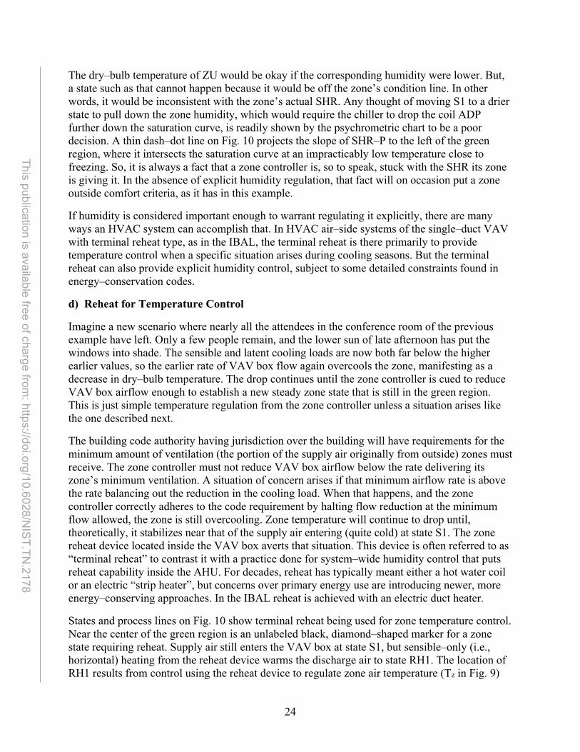
24


IST.TN.2178

The dry–bulb temperature of ZU would be okay if the corresponding humidity were lower. But, a state such as that cannot happen because it would be off the zone’s condition line. In other words, it would be inconsistent with the zone’s actual SHR. Any thought of moving S1 to a drier state to pull down the zone humidity, which would require the chiller to drop the coil ADP further down the saturation curve, is readily shown by the psychrometric chart to be a poor decision. A thin dash–dot line on Fig. 10 projects the slope of SHR–P to the left of the green region, where it intersects the saturation curve at an impracticably low temperature close to freezing. So, it is always a fact that a zone controller is, so to speak, stuck with the SHR its zone is giving it. In the absence of explicit humidity regulation, that fact will on occasion put a zone outside comfort criteria, as it has in this example.

If humidity is considered important enough to warrant regulating it explicitly, there are many ways an HVAC system can accomplish that. In HVAC air–side systems of the single–duct VAV with terminal reheat type, as in the IBAL, the terminal reheat is there primarily to provide temperature control when a specific situation arises during cooling seasons. But the terminal reheat can also provide explicit humidity control, subject to some detailed constraints found in energy–conservation codes.

d) Reheat for Temperature Control

Imagine a new scenario where nearly all the attendees in the conference room of the previous example have left. Only a few people remain, and the lower sun of late afternoon has put the windows into shade. The sensible and latent cooling loads are now both far below the higher earlier values, so the earlier rate of VAV box flow again overcools the zone, manifesting as a decrease in dry–bulb temperature. The drop continues until the zone controller is cued to reduce VAV box airflow enough to establish a new steady zone state that is still in the green region. This is just simple temperature regulation from the zone controller unless a situation arises like the one described next.

The building code authority having jurisdiction over the building will have requirements for the minimum amount of ventilation (the portion of the supply air originally from outside) zones must receive. The zone controller must not reduce VAV box airflow below the rate delivering its zone’s minimum ventilation. A situation of concern arises if that minimum airflow rate is above the rate balancing out the reduction in the cooling load. When that happens, and the zone controller correctly adheres to the code requirement by halting flow reduction at the minimum flow allowed, the zone is still overcooling. Zone temperature will continue to drop until, theoretically, it stabilizes near that of the supply air entering (quite cold) at state S1. The zone reheat device located inside the VAV box averts that situation. This device is often referred to as “terminal reheat” to contrast it with a practice done for system–wide humidity control that puts reheat capability inside the AHU. For decades, reheat has typically meant either a hot water coil or an electric “strip heater”, but concerns over primary energy use are introducing newer, more energy–conserving approaches. In the IBAL reheat is achieved with an electric duct heater.

States and process lines on Fig. 10 show terminal reheat being used for zone temperature control. Near the center of the green region is an unlabeled black, diamond–shaped marker for a zone state requiring reheat. Supply air still enters the VAV box at state S1, but sensible–only (i.e., horizontal) heating from the reheat device warms the discharge air to state RH1. The location of RH1 results from control using the reheat device to regulate zone air temperature (Tz in Fig. 9)

25


IST.TN.2178

instead of the usual way of regulating airflow rate. Note the low cooling load results in a short, shallowly sloped (i.e., SHR near 1.0) mixing process to the zone state marked by the black diamond. The controller raises the discharge temperature until RH1 intersects a projection of the SHR drawn through Z1. When Tz is no longer decreasing, RH1 is at that intersection and is held there. Without reheat, that same process line would begin instead at S1, placing the zone state far below acceptable temperatures.

Reheat needs to be understood for what it really is, the control system adding sensible cooling load to the zone so minimum ventilation requirements can be supported without overcooling. Unless the AHU is in a condition known as “free cooling”, such a control action is a form of “simultaneous heating and cooling” according to building codes that dictate energy conservation. Reheat quite blatantly consumes new energy to restore old energy the chiller plant already worked to remove from the AHU coil and supply air, a practice that understandably is not treated lightly by energy–conservation codes. Code authorities typically preclude most types of buildings from using reheat unless specific system provisions and control prerequisites are met. The system provisions have to do with AHU size and energy sources, and as such are not real–time control concerns. The control prerequisites generally allow reheat once airflow is turned down to 50 % or less of the design value, or turned down to the minimum ventilation rate, whichever is highest. IBAL experiments on control methods that include reheat are designed to satisfy an appropriate energy code when implementing reheat so that the experiments will be realistic.

e) Reheat for Humidity Control

If a humidity sensor is added to the thermostatic controls, terminal reheat can be used for explicit control of zone humidity. This applies to buildings where specific humidity levels are necessary to satisfy process needs, such as museums, medical or pharmacy facilities, ice arenas, or cold storage. Or, it can apply to spaces where a priority is given to averting failures of implicit humidity control, such as happened in the example discussed earlier where a large conference room became too cool and damp. Referring back to Fig. 10 we look at that example again, but now with reheat used for humidity control.

Recall that the cooling load in the conference room changed such that SHR steepened from SHR–D to SHR–P. But now, the humidity sensor is used by the zone controller to apply reheat and keep the zone state in the green region. The diagram in Fig. 10 shows the reheat process extending to the same discharge air state as for the temperature control example, state RH1. The zone air mixing process now begins at RH1 and, having the same SHR–P slope as it does without reheat, it now results in the zone state staying at Z1. In actual practice it is best to minimize reheat energy, so the zone controller would place RH1 more to the left. That translates the mixing process line to the left, still at the same slope, which places the zone at a more economical state, slightly cooler and higher in relative humidity than Z1, but still in the green region.

The code prerequisites seen in the temperature control case still apply. When the cooling load decreases and before reheat is allowed, the zone controller must first turn down discharge airflow in an attempt to find a new zone state in the green region.

26


IST.TN.2178

f) Winter Design Diagram

Looking now at the winter design diagram on Fig. 10, the outdoor air drawn in by the AHU is at state OWD, and the zone air is to be at state Z2. As was done on the summer design diagram, simplifications are made for clarity. OWD is linked to Z2 by the process of mixing ventilation and recirculation air in the AHU mixing box. The mixing box state is M2. There is no coil curve for this condition; the coil is inactive. State M2 is sufficiently cold to provide cooling where it is required. However, if OWD is sufficiently cold, as is the case here, and particularly when the outdoor airflow rate is high, M2 might be below the dry–bulb temperature wanted for the supply air.

Common practice in a single–duct VAV design is to calculate the supply air dry–bulb temperature based on the summer design criteria (as state S1 was) and then have the AHU control prevent it from going lower than that, even in winter. The discharge velocity, throw, and pattern characteristics of the many air diffusers throughout all the zones are selected to avoid creating cold, uncomfortable drafts given air at the design temperature. An AHU controller allowing colder supply temperatures would subvert that intention. This is one reason, although not the primary reason, the AHU has a “preheat” capability. The primary reason is that air entering the AHU could be at a temperature close enough to freezing to be a hazard to the cooling coil, especially when the coil is inactive. AHU preheat brings the supply air from M2 to S2, which is essentially S1 but at a much lower moisture content resulting from the dryness of winter outdoor air. In this simplified presentation, S2 is the air temperature leaving the AHU and the air temperature discharged into the zone by the VAV box.

The solid black line depicting the zone air mixing process from S2 to Z2 has a slope corresponding to the zone’s current SHR. It is notably steeper (i.e., smaller proportion of sensible load) than SHR–D in the summer diagram, since in winter a zone (whether internal or external) has no sensible cooling load to pick up from envelope elements such as walls and windows. In fact, an external zone in winter has the opposite, an energy loss in the form of an envelope heating load. So, the winter diagram seen here applies approximately to either internal or external zones. In addition, despite being about a winter condition, this diagram is like one for a summer condition, being basically a cooling load diagram. It depicts what happens in a single–duct VAV with terminal reheat system, and such systems are basically cooling–only systems, leaving the heating load to be handled by separate perimeter heat systems.

The zone controller modulates the VAV box damper to match the airflow to that required to pick up the zone cooling load. If that amount is below the minimum rate required for ventilation, the controller must also activate reheat, otherwise the ventilation adds to the zone heating load. The diagram shows reheat creating state RH2, and zone mixing picking up a cooling load between RH2 and Z2. Occupied and lit internal zones will present cooling loads year–round, but for external zones the situation is not as certain and may vary between individual zones depending on the degree of external exposure.

If the cooling load in an external zone is low enough to be offset by the zone’s envelope heating load, the zone controller still admits required ventilation air and applies reheat to it as described earlier. But the reheat device is not intended for handling any of a zone’s heating load. If it did handle the heating load, the VAV box airflow would have to turn up to a value that meets the heating load given the temperature rise across the reheat device, posing an energy code violation

27


IST.TN.2178

as well as an illogical design requirement. Handling heating loads with a separate perimeter system means the temperature difference to be addressed in meeting that load is the zone air temperature versus the outdoor air temperature, not the supply air temperature versus the outdoor air temperature, the latter being a difference of about 11 °C (20 °F) more. Further, the entire zone air system including the AHU would need to be much larger to handle heating the zone’s physical space instead of merely tempering its ventilation. So, instead, two separate systems of temperature control loops and heating devices are used, one to meet a zone’s reheat needs and the other for its heating load. They functionally need each other but can be logically independent of each other. Each can hold its setpoint because of the effect from the other, but it is not necessary to encode that interdependency into the controllers.

g) Humidification

Humid seasons are those where the absolute moisture content outdoors exceeds values that result in acceptable relative humidity indoors, and we have already shown how single–duct VAV with terminal reheat systems can either implicitly or explicitly handle that. During drier seasons such as winter, the so–called “moisture drive” is reversed, and some form of humidification process is often required. Looking at the winter design diagram of Fig. 10, one might wonder where the humidity required to keep zone state Z2 in the green region comes from. There are people in the zone, which presents some latent load that causes the SHR to slope up somewhat. But is that ever going to be sufficient to get Z2 into the green region, especially given the low moisture at S2 and the amount of sensible pick up that takes place? The answer to that is: “Probably not.” So, a humidification process not shown on the Fig. 10 winter diagram is needed to get the states to where they are on the diagram. The humidification process could be a humidifier in the AHU, in the zone supply ductwork, or somewhere in the occupied space. The former two installations can be represented on the diagram as lines upwards from S2 or RH2, respectively. The latter installation, a “room humidifier”, is like the perimeter heat of the temperature control example in that its effects are evident on the diagram, but its process cannot be meaningfully shown on it.

3.4. Zone Simulation in the IBAL

This section will talk in detail about how loads are generated in the IBAL, and the following section will discuss how the zone cooling needs are met in the IBAL. As mentioned in the Introduction, due to the constraints of the physical space in the NIST building housing the IBAL, the zones are simulated via modules designed for the purpose. The zone simulators contain a 5 kW electric heater to generate sensible loads and a steam spray humidifier (SSH) to generate latent loads. Control of the sensible load is achieved by sending the SCR (silicon–controlled rectifier) controller a current between 4.5 mA and 14 mA and the latent load is controlled by sending a steam control valve a signal between 2 V and 10 V. The IBAL does not consider heating loads at this time, though it does have some limited ability to generate them if that capability is desired in the future.

Ideally, the sensible load generated by the heater would equal the power consumption of the heater, i.e., 100 % efficiency. This is a very consistent and clean measurement, so it is ideal for PI control. However, in practice there are parasitic sensible loads that need to be considered. The main source of a parasitic load is the SSH. The SSH has a steam jacket to minimize condensation and dripping, which means that even when the control valve is closed, and there is therefore no stream being sprayed into the airstream, there is steam flowing in the jacket. Although there is a

28


IST.TN.2178

layer of insulation on the SSH, there is still heat transfer to the airstream by convection and conduction. In addition, when a latent load is required and steam is sprayed into the airstream, the steam increases the air temperature by a small amount. For this reason, rather than using the power measurement as the process variable, the process variable is the sensible load calculated in the airstream (Fig. 11), referred to as the pickup (i.e., the sensible energy transferred to the airstream), and the current is the control variable. The control is similar for the latent load, where the process variable is the latent load calculated in the airstream and the control variable is the voltage to the control valve (Fig. 12). Recall that the PI timestep in the IBAL is 10 s; this is also the overall default control loop timestep. All control logic is implemented in a custom LabVIEW program.

Fig. 11. PI loop for the sensible load in the zone.

Kp

KI 1𝑠𝑠

+ –

Heater

Controller

out

Humidifier

in

qsensible

qsensible,SP

29


IST.TN.2178

Fig. 12. PI loop for the latent load in the zone.

The sensible and latent loads picked up by the airstream, qsensible and qlatent, are calculated based on equations adapted from Chapter 1 of the ASHRAE Handbook of Fundamentals [9]. The specific heat of air (cp) and the inlet (Tin) and outlet (Tout) temperatures are required for the sensible load calculation (Eq. (12)) while the inlet (ωin) and outlet (ωout) humidity ratios, calculated from the measured air temperature and relative humidity, are required for the latent load calculation (Eq. (13)). In Eq. (13), the constant 2470 has units of kJ/kg and is the latent heat of vaporization of water at 15 °C (59 °F). Both calculations require the mass flow rate of the dry air (�̇�𝑚𝑑𝑑𝑟𝑟). The lab measures the volumetric airflow rate of the moist air (∀ ̇ 𝑟𝑟), which is divided by the specific volume of dry air (𝜈𝜈𝑑𝑑𝑟𝑟), as shown in Eq. (14), to calculate �̇�𝑚𝑑𝑑𝑟𝑟.

𝑞𝑞𝑏𝑏𝑟𝑟𝑚𝑚𝑏𝑏𝐻𝐻𝑏𝑏𝑠𝑠𝑟𝑟[𝑘𝑘𝑘𝑘] = ��𝑐𝑐𝑝𝑝𝑇𝑇�𝐿𝐿𝑜𝑜𝑟𝑟 − �𝑐𝑐𝑝𝑝𝑇𝑇�𝐻𝐻𝑚𝑚� �̇�𝑚𝑑𝑑𝑟𝑟 (12)

𝑞𝑞𝑠𝑠𝑟𝑟𝑟𝑟𝑟𝑟𝑚𝑚𝑟𝑟[𝑘𝑘𝑘𝑘] = 2470 �̇�𝑚𝑑𝑑𝑟𝑟(𝜔𝜔𝐿𝐿𝑜𝑜𝑟𝑟 − 𝜔𝜔𝐻𝐻𝑚𝑚) (13)

�̇�𝑚𝑑𝑑𝑟𝑟[𝑘𝑘𝑘𝑘 𝑠𝑠⁄ ] =∀ ̇ 𝑟𝑟𝜈𝜈𝑑𝑑𝑟𝑟

(14)

The load setpoints, qsensible,SP and qlatent,SP, are supplied to the controller by the user (or an external program). The current values of the PI parameters for the sensible and latent load controllers, respectively, are given in Table 2 and Table 3.

Kp

KI 1𝑠𝑠

+ –

Heater

Controller

out

Humidifier

in

qlatent

qlatent,SP

30


IST.TN.2178

Table 2. Current values of the tunable PI parameters for the zone sensible load control.

Name Current Value Kp 0.35 KI 0.003 Kd 0 SPHigh 5300 W SPLow 0 W uBias 0 A 1 EUHigh 0.014 A EULow 0.0045 A

Table 3. Current values of the tunable PI parameters for the zone latent load control.

Name Current Value Kp 0.5 KI 0.0075 Kd 0 SPHigh 2000 W SPLow 0 W uBias 0.4 A 1 EUHigh 2 V EULow 10 V

This control approach works under the assumption that the controller responds quickly relative to the dynamics of the inlet air conditions (temperature and airflow rate). To date this has been the case, but it is possible that the control approach will have to be adjusted in the future to rely less on potentially transitory system measurements. In a real building, the load generated by a computer, for example, is not dependent on the temperature of the air entering the zone, but in this control system it is.

3.5. Zone Control in the IBAL

As discussed in Sec. 3.3.1, the state of the zone air is most directly regulated by the control devices in the VAV box, the damper and the heater, which is electric in the IBAL. The next sections discuss the details of the local control loops that determine the operation of these devices. Section 3.5.3 presents a supervisory controller for calculating the setpoints used in the local control loops. That controller is one target for intelligent agents.

31


IST.TN.2178

3.5.1. Volume Control

Figure 13 shows the PI loop for control of the VAV damper. The process variable is the airflow rate, ∀̇𝑟𝑟, and the setpoint, ∀̇𝑆𝑆𝑆𝑆, is calculated based on the difference between the zone temperature, Tz, and the zone setpoint, Tz,SP (Sec. 3.5.3). The control variable is the damper position. The current values of the PI parameters for all VAV damper controllers are given in Table 4. The damper control signal increases to increase airflow, so this is a direct acting controller.

Fig. 13. PI loop for the VAV damper position.

Table 4. Current values of the tunable PI parameters for VAV damper control. Name Current Value Kp 0.2 KI 0.01 Kd 0 SPHigh 1699 m3/hr (1000 cfm) SPLow 0 uBias 1 A 1 EUHigh 10 V EULow 2 V

∀̇

Kp

K

1𝑠𝑠

+ –

Heater

Controller

Damper

∀̇𝑆𝑆𝑆𝑆

32


IST.TN.2178

3.5.2. Reheat

If the airflow has been throttled to a minimum and the zone is still too cold, then the electric heater in the VAV can be used to heat the air entering the zone (see Sec. 3.3.3d). The process variable is the temperature leaving the VAV, Td, and the control variable is a control signal sent to the heater. The current values of the PI parameters for all VAV reheat controllers are given in Table 5. The air temperature increases in proportion to the reheat control signal, so this is a direct acting controller.

Fig. 14. VAV reheat PI controller.

Table 5. Current values of the tunable PI parameters for VAV reheat control.

Name Current Value Kp 2 KI 0.01 Kd 0 SPHigh 32 °C (90 °F) SPLow –1.1 °C (30 °F) uBias 0 A 1 EUHigh 10 V EULow 0 V

3.5.3. Airflow and Temperature Reset

∀̇𝑆𝑆𝑆𝑆 and Td,SP can be constant, but, if they are reset, the volume and temperature of air delivered will better match the needs of the zones and can result in a decrease in fan and heater power

Kp

K

1𝑠𝑠

+ –

Heater

Controller

Damper

Td,SP

Td

33


IST.TN.2178

consumption, respectively. These two controllers are intertwined and therefore are presented together.

The dual maximum reset scheme, called such because there are maximum heating and cooling airflow rates, is presented in Refs [11, 12]. The basic concept is to divide the operation of the system into four parts:

1. Cooling mode: calculate the airflow rate between a minimum and maximum in proportion to the magnitude of the cooling loop signal

2. Deadband: the cooling and heating loop signals are at their minimum; the airflow rate is held at the minimum and there is no reheat

3. Heating mode: reheat – set the temperature leaving the VAV (i.e., the reheat temperature setpoint) up to a maximum, Td,max, in proportion to the error in the zone temperature. The airflow is held at the minimum.

4. Heating mode: airflow – once maximum reheat has been reached, set the airflow rate in proportion to the error in the zone temperature, limited to between the minimum and the maximum airflow rate in heating mode.

In general, the heating and cooling loop signals range from 0 % (off) to 100 % (full on). In the case of the IBAL, if the airflow rate is at its maximum and the damper is wide open, the cooling loop signal is 100 %.

This approach is adapted in the IBAL with some changes. One major difference is that the deadband mode is not explicitly implemented. Instead, the cooling mode extends through the deadband. In addition, the airflow rate is not set in proportion to the cooling loop signal but is instead adjusted based on the mode and the error in the zone temperature. Figure 15 graphically shows the operation of the controller and Table 7 defines the variables in the graphs.

34


IST.TN.2178

Fig. 15. Sketch of the airflow and temperature profiles for control.

The operating mode (i.e. heating or cooling) is determined as shown in Fig. 16; Table 6 defines the variables used in the calculations that are not defined in Table 7. The system initially enters heating mode if the zone temperature is less than the setpoint by at least the heating deadband (dbheat) and the airflow rate is at the minimum (∀̇𝑚𝑚𝐻𝐻𝑚𝑚). Once it is in heating mode, it remains in that mode if the reheat control signal (uvav,heat) is greater than zero or the setpoint temperature is greater than the temperature entering the VAV, indicating a need for heating. If the system is not in heating mode, the default mode is cooling mode. When the airflow setpoint is near the minimum and the reheat control signal is zero, the system is in a deadband between the heating and cooling loop, but for simplicity in the implementation, this mode is lumped into the cooling mode. The setpoints can only be updated every n timesteps, as tracked by counter N.

∀̇𝑚𝑚𝑟𝑟𝑚𝑚,𝑠𝑠𝐿𝐿𝐿𝐿𝑠𝑠

∀̇𝑚𝑚𝑟𝑟𝑚𝑚,ℎ𝑟𝑟𝑟𝑟𝑟𝑟

∀̇𝑚𝑚𝐻𝐻𝑚𝑚

3 2 1

Heating mode: reheat

Cooling mode Heating mode: airflow

Td,max

3 2 1

Heating mode: reheat

Cooling mode Heating mode: airflow

35


IST.TN.2178

Fig. 16. Pseudocode for determining the operating mode in the VAV airflow and temperature reset controller.

Table 6. Variables in the flow and temperature reset controller.

Variable Description Tz Measured zone temperature Tz,SP Zone temperature setpoint Td,SP Reheat setpoint TVAV,in Temperature at the inlet to the VAV mode Operating mode – either cooling or heating ∀̇𝑆𝑆𝑆𝑆 Airflow rate setpoint uvav,heat Current VAV reheat control signal Nreset Number of timesteps since the last reset

Table 7. Tunable variables in the flow and temperature reset controller.

Variable Description Current Value n Number of timesteps between SP changes 9 ∀̇max,cool Maximum airflow rate in cooling 0.47 m3/s (1000 cfm) ∀̇max,heat Maximum airflow rate in heating 0.23 m3/s (500 cfm)

dbheat Heating deadband 0.56 °C (1 °F) ∀̇min Minimum airflow rate 0.12 m3/s (250 cfm) Td,max Maximum reheat temperature 32.2 °C (90 °F)

VAV Cooling or Heating Mode: Determine the mode of operation for the VAV dual maximum controller

vavMode() first call: N = 0; mode = cooling 1: N = N + 1 2: if N > n

3: N = 0 4: if Tz < Tz,SP – db and F < 1.02*Fmin 5: mode = heating 6: else if mode == heating and Tz < Tz,SP – db and Td,sp > 0.98*Td,max 7: mode = heating 8: else if mode == heating and uheat,vav > 0.001 9: mode = heating 10: else if mode == heating and Td,sp > Tvav,in + 0.8 °C (1.5 °F) 11: mode = heating 12: else 13: mode = cooling 14: endif 15: endif 15: return mode

36


IST.TN.2178

Once the mode has been determined, the temperature and airflow setpoints are calculated as follows:

• Cooling mode o ∀̇𝑆𝑆𝑆𝑆 calculated from a PI loop (Fig. 17) o Td,SP = TVAV,in – 2.8 °C (5 °F)

• Heating mode – reheat o Td,SP calculated from a PI loop (Fig. 18) o ∀̇𝑆𝑆𝑆𝑆 = ∀̇𝑚𝑚𝐻𝐻𝑚𝑚,𝑠𝑠𝐿𝐿𝐿𝐿𝑠𝑠

• Heating mode – airflow o Td,SP = Td,max o ∀̇𝑆𝑆𝑆𝑆 calculated from a PI loop (Fig. 17)

The tunable parameters for the PI controllers for airflow reset and temperature reset are in Table 8 and Table 9, respectively.

Fig. 17. PI loop that calculates ∀̇𝑆𝑆𝑆𝑆 from the zone temperature and feeds to the VAV damper control signal. This loop is used in cooling mode or in heating mode if the reheat temperature is at its maximum value.

Kp

KI 1𝑠𝑠

+ –

Heater

Controller

Tz,SP

Tz

Humidifier

Kp

KI 1𝑠𝑠

Heater

Controller

Damper

∀̇𝑆𝑆𝑆𝑆

+ –

VAV Zone

∀̇𝑟𝑟

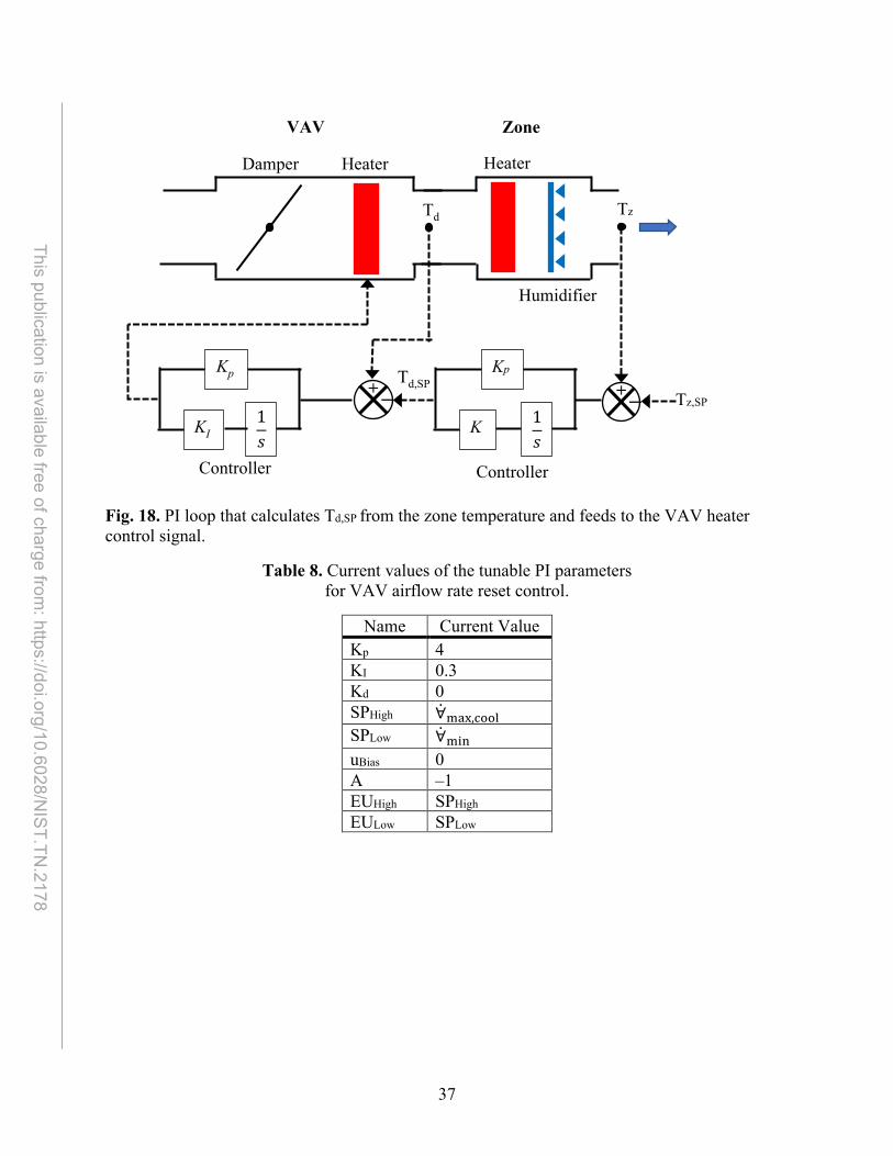
37


IST.TN.2178

Fig. 18. PI loop that calculates Td,SP from the zone temperature and feeds to the VAV heater control signal.

Table 8. Current values of the tunable PI parameters for VAV airflow rate reset control.

Name Current Value Kp 4 KI 0.3 Kd 0 SPHigh ∀̇max,cool SPLow ∀̇min uBias 0 A –1 EUHigh SPHigh EULow SPLow

Kp

K

1𝑠𝑠

+ –

Heater

Controller

Tz,SP

Tz

Humidifier

Kp

KI 1𝑠𝑠

Heater

Controller

Damper

Td,SP

Td

+ –

VAV Zone

38


IST.TN.2178

Table 9. Current values of the tunable PI parameters for VAV temperature reset control.

Name Current Value Kp –2 KI 0.05 Kd 0 SPHigh Td,max SPLow 4.4 °C (40 °F) uBias 0 A 1 EUHigh SPHigh EULow SPLow

39


IST.TN.2178

AHU Controller

As discussed in Sec. 3.3.1, the AHU provides a head of preconditioned air to the VAV boxes. There are three primary controllers for the AHU in the IBAL. The first controller determines the positions of the dampers at the inlet to the AHU (i.e., mixing box), the second controller determines the temperature of the air at the outlet of the AHU, and the third controller directly determines the head of air supplied to the VAV from the AHU. This section also presents two supervisory controllers, one that determines the setpoint for the air temperature and one that determines the setpoint for the head of the air. These controllers work together to provide air of the correct temperature and volume to meet the needs of the zones. Recall that the IBAL has two AHUs, and although they use the same control logic, the specific sensors and actuators are unique to each AHU.

4.1. Air Dampers

The air entering the AHU is a mix of return air (RA) from the zone and emulated outdoor air (EOA) from the weather emulator. The EOA is the ventilation air discussed in Sec. 3.2.1. The percent of the total air entering the zone that is emulated outdoor air, Peoa, is controlled by the PI loop shown in Fig. 19. The setpoint, Peoa,SP, is currently user generated. In the IBAL, this controller would be used to enable the economizer mode of the AHU (Sec. 3.3.1) by changing the setpoint, but the logic to enable and implement economizer mode is not currently implemented.

Fig. 19. PI loop that modulates the emulated outdoor air damper to achieve the percent emulated outdoor air setpoint, Peoa,SP.

Peoa,SP

Kp

KI 1𝑠𝑠

+ –

Emulated Outdoor Air Damper

Controller

Return Air Damper

Exhaust Damper

𝑆𝑆𝑟𝑟𝐿𝐿𝑟𝑟 =∀̇𝑟𝑟𝐿𝐿𝑟𝑟

∀̇𝑟𝑟𝐿𝐿𝑟𝑟 + ∀̇𝑟𝑟𝑟𝑟

∀̇𝑟𝑟𝑟𝑟

∀̇𝑟𝑟𝐿𝐿𝑟𝑟 AHU VAV ZONE

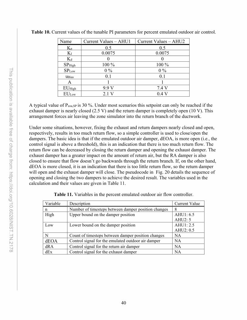
40


IST.TN.2178

Table 10. Current values of the tunable PI parameters for percent emulated outdoor air control.

Name Current Values – AHU1 Current Values – AHU2 Kp 0.5 0.5 KI 0.0075 0.0075 Kd 0 0

SPHigh 100 % 100 % SPLow 0 % 0 % uBias 0.1 0.1 A 1 1

EUHigh 9.9 V 7.4 V EULow 2.1 V 0.4 V

A typical value of Peoa,SP is 30 %. Under most scenarios this setpoint can only be reached if the exhaust damper is nearly closed (2.5 V) and the return damper is completely open (10 V). This arrangement forces air leaving the zone simulator into the return branch of the ductwork. Under some situations, however, fixing the exhaust and return dampers nearly closed and open, respectively, results in too much return flow, so a simple controller is used to close/open the dampers. The basic idea is that if the emulated outdoor air damper, dEOA, is more open (i.e., the control signal is above a threshold), this is an indication that there is too much return flow. The return flow can be decreased by closing the return damper and opening the exhaust damper. The exhaust damper has a greater impact on the amount of return air, but the RA damper is also closed to ensure that flow doesn’t go backwards through the return branch. If, on the other hand, dEOA is more closed, it is an indication that there is too little return flow, so the return damper will open and the exhaust damper will close. The pseudocode in Fig. 20 details the sequence of opening and closing the two dampers to achieve the desired result. The variables used in the calculation and their values are given in Table 11.

Table 11. Variables in the percent emulated outdoor air flow controller.

Variable Description Current Value n Number of timesteps between damper position changes 8 High Upper bound on the damper position AHU1: 6.5

AHU2: 5 Low Lower bound on the damper position AHU1: 2.5

AHU2: 0.5 N Count of timesteps between damper position changes NA dEOA Control signal for the emulated outdoor air damper NA dRA Control signal for the return air damper NA dEx Control signal for the exhaust damper NA

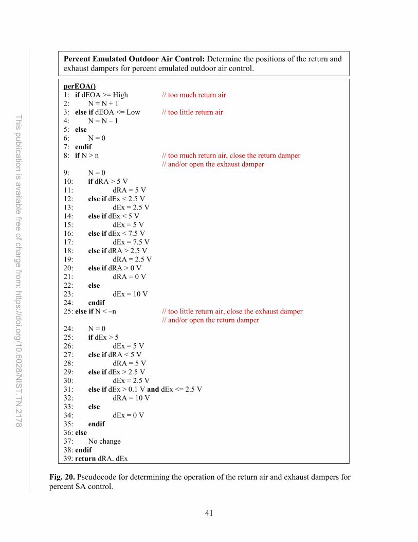
41


IST.TN.2178

Fig. 20. Pseudocode for determining the operation of the return air and exhaust dampers for percent SA control.

Percent Emulated Outdoor Air Control: Determine the positions of the return and exhaust dampers for percent emulated outdoor air control. perEOA() 1: if dEOA >= High // too much return air 2: N = N + 1 3: else if dEOA <= Low // too little return air 4: N = N – 1 5: else 6: N = 0 7: endif 8: if N > n // too much return air, close the return damper // and/or open the exhaust damper 9: N = 0 10: if dRA > 5 V 11: dRA = 5 V 12: else if dEx < 2.5 V 13: dEx = 2.5 V 14: else if dEx < 5 V 15: dEx = 5 V 16: else if dEx < 7.5 V 17: dEx = 7.5 V 18: else if dRA > 2.5 V 19: dRA = 2.5 V 20: else if dRA > 0 V 21: dRA = 0 V 22: else 23: dEx = 10 V 24: endif 25: else if N < –n // too little return air, close the exhaust damper // and/or open the return damper 24: N = 0 25: if dEx > 5 26: dEx = 5 V 27: else if dRA < 5 V 28: dRA = 5 V 29: else if dEx > 2.5 V 30: dEx = 2.5 V 31: else if dEx > 0.1 V and dEx <= 2.5 V 32: dRA = 10 V 33: else 34: dEx = 0 V 35: endif 36: else 37: No change 38: endif 39: return dRA, dEx

42


IST.TN.2178

4.2. Supply Air Temperature

The temperature of the supply air (i.e., the conditioned air leaving the AHU) is determined primarily by the position of the cooling coil (CC) valve. If the valve is more open, then there is greater flow of coolant through the CC and the air temperature will decrease, so this is an indirect acting loop. Figure 21 shows a basic schematic of this control loop, where Tsa is the supply air temperature and Tsa,SP is the setpoint. In Sec. 3.3.3b there is a discussion about the temperature of the metal and the theoretical ADP temperature, but this controller ignores those complexities and instead modulates the cooling coil valve to control the temperature of the air downstream of the AHU fan, which is the temperature of the air entering the VAV boxes.

Fig. 21. PI loop that modulates the cooling coil valve to bring the supply air temperature, Tsa, to the setpoint, Tsa,SP.

The current values of the PI parameters for the supply air temperature controllers of the two AHUs are given in Table 12.

Tsa

Kp

KI 1𝑠𝑠

+ – Tsa, SP

Heater Cooling Coil

Fan

Cooling Coil Valve

Controller

43


IST.TN.2178

Table 12. Current values of the tunable PI parameters for AHU supply air temperature control.

Name Current Value Kp 3 KI 0.015 Kd 0 SPHigh 21 °C (70 °F) SPLow –1 °C (30 °F) uBias 0 A –1 EUHigh 6.5 V EULow 2 V

4.3. Supply Air Temperature Reset

Although Tsa,SP can be constant, supply air temperature (SAT) reset is a strategy that can lead to energy savings by updating Tsa,SP based on the existing state of the system. For example, if the building load decreases it may be possible to meet that load with air at a higher temperature, which can translate to a reduction in chiller power consumption (see Sec. 5.3.1). The controller logic is outlined in Fig. 22 and the parameters are defined in Table 13. The concept is based on the logic presented in the Advanced Variable Air Volume Systems Design Guide [13].

44


IST.TN.2178

Table 13. Tunable variables in the supply air temperature reset controller.

Variable Description Value n Number of timesteps between SP changes 12 nreq Number of requests for cooling required for a SP decrease 2 V Threshold to indicate that the dampers are open, indicating cooling

is needed 15 V

Hz Threshold to indicate that the fan is delivering a large volume of

55 Hz ∆ The amount by which to change the SP 0.1 °C (0.2 °F) Tmax The maximum value of the SP 18.3 °C (65 °F) Tmin The minimum value of the SP 10 °C (50 °F) Tdesign The design value of the SP 12.8 °C (55 °F) N Count of timesteps between SP changes ≥ 0 Nreq Number of requests for cooling during the interval ≥ 0 rh1 Status of reheat for the first VAV 0 (off) or 1 (on) rh2 Status of reheat for the second VAV 0 (off) or 1 (on) rh Status of reheat for both VAVs served by the AHU ≥ 0 d1 Position of the damper in the first VAV 2 V ≤ d1 ≤ 10 V d2 Position of the damper in the second VAV 2 V ≤ d2 ≤ 10 V d Sum of the damper positions vfd Fan speed 15 Hz ≤ vfd ≤ 60 Hz VCC Cooling coil valve position Low ≤ VCC ≤ High Low Minimum position of the cooling coil valve 2 V High Maximum position of the cooling coil valve 6.5 V

The controller has two parts: 1) determine if cooling is requested and 2) adjust the SP if necessary. A request for cooling occurs if the VAV dampers for a given AHU are both sufficiently open, the fan speed is sufficiently high, and there is no reheat. If there have been no requests for cooling, this may indicate that the air temperature is too low, and therefore Tsa,SP increases by ∆. If the number of requests for cooling exceeds a threshold, this is an indication that the air temperature is too high, and the SP decreases by ∆. If neither of these situations is true, the SP remains unchanged.

In addition to possible changes to the values of the parameters in Table 13, there are other changes that might be made to improve this controller. For example, reference [13] recommends reducing the SP to its minimum value (Tmin) when the outdoor air temperature (TOA) is greater than or equal to 21.1 °C (70 °F), and then increasing the temperature linearly as TOA decreases, eventually reaching Tmax. The advantage of this approach is that the SP is likely to reach a near optimal value more quickly, but the value of TOA where the temperature should be at Tmin or Tmax may be not only a function of temperature, but also humidity, so this result may vary with climate zone and have an impact on the system beyond just the cooling coil control. For example, the system may require dehumidification, but that may lower the air temperature below SP, which will then require reheat, which may or may not still save energy.

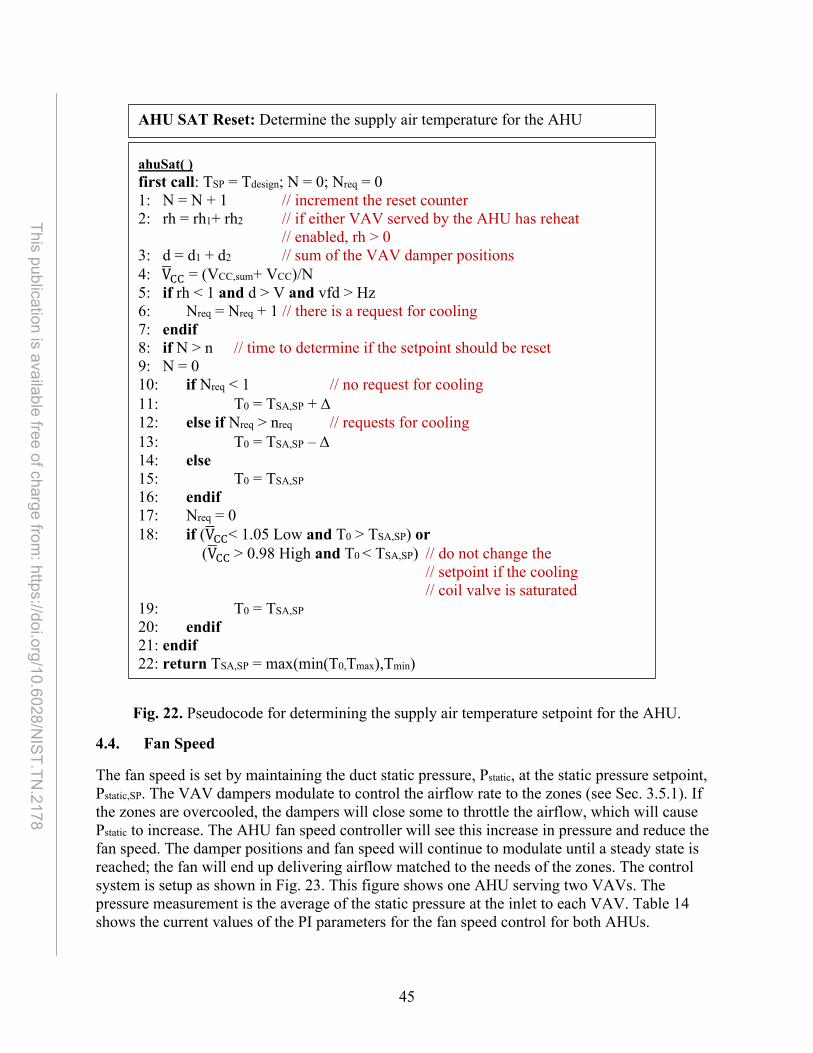
45


IST.TN.2178

Fig. 22. Pseudocode for determining the supply air temperature setpoint for the AHU.

4.4. Fan Speed

The fan speed is set by maintaining the duct static pressure, Pstatic, at the static pressure setpoint, Pstatic,SP. The VAV dampers modulate to control the airflow rate to the zones (see Sec. 3.5.1). If the zones are overcooled, the dampers will close some to throttle the airflow, which will cause Pstatic to increase. The AHU fan speed controller will see this increase in pressure and reduce the fan speed. The damper positions and fan speed will continue to modulate until a steady state is reached; the fan will end up delivering airflow matched to the needs of the zones. The control system is setup as shown in Fig. 23. This figure shows one AHU serving two VAVs. The pressure measurement is the average of the static pressure at the inlet to each VAV. Table 14 shows the current values of the PI parameters for the fan speed control for both AHUs.

AHU SAT Reset: Determine the supply air temperature for the AHU

ahuSat( ) first call: TSP = Tdesign; N = 0; Nreq = 0 1: N = N + 1 // increment the reset counter 2: rh = rh1+ rh2 // if either VAV served by the AHU has reheat

// enabled, rh > 0 3: d = d1 + d2 // sum of the VAV damper positions 4: V�CC = (VCC,sum+ VCC)/N 5: if rh < 1 and d > V and vfd > Hz 6: Nreq = Nreq + 1 // there is a request for cooling 7: endif 8: if N > n // time to determine if the setpoint should be reset 9: N = 0 10: if Nreq < 1 // no request for cooling 11: T0 = TSA,SP + ∆ 12: else if Nreq > nreq // requests for cooling 13: T0 = TSA,SP – ∆ 14: else 15: T0 = TSA,SP

16: endif 17: Nreq = 0 18: if (V�CC< 1.05 Low and T0 > TSA,SP) or

(V�CC > 0.98 High and T0 < TSA,SP) // do not change the // setpoint if the cooling // coil valve is saturated

19: T0 = TSA,SP

20: endif 21: endif 22: return TSA,SP = max(min(T0,Tmax),Tmin)

46


IST.TN.2178

Fig. 23. PI loop that modulates the fan speed to bring the duct static pressure, Pstatic, to the static pressure setpoint, Pstatic,SP.

Table 14. Current values of the tunable PI parameters for AHU fan speed control.

Name Current Value Kp 0.25 KI 0.01 Kd 0 SPHigh 996 Pa (4 inH2O) SPLow 0 Pa (0 inH2O) uBias 0.5 A 1 EUHigh 60 Hz EULow 15 Hz

4.5. Static Pressure Reset

Pstatic,SP can be constant, but performance gains can be achieved by using static pressure reset to increase or decrease the setpoint based on the real–time needs of the system [13]. The tunable variables of the controller are in Table 15, and Fig. 24 is pseudocode of the logic for the controller. Each AHU serves two VAVs with dampers d1 and d2; if only one VAV is in use, then the logic shown in the figure still works, but it only considers the VAV that is in use.

Pstatic

Kp

KI 1𝑠𝑠

+ – Pstatic, SP

Heater Cooling Coil

Fan

Controller

Heater

Heater

dA

dB

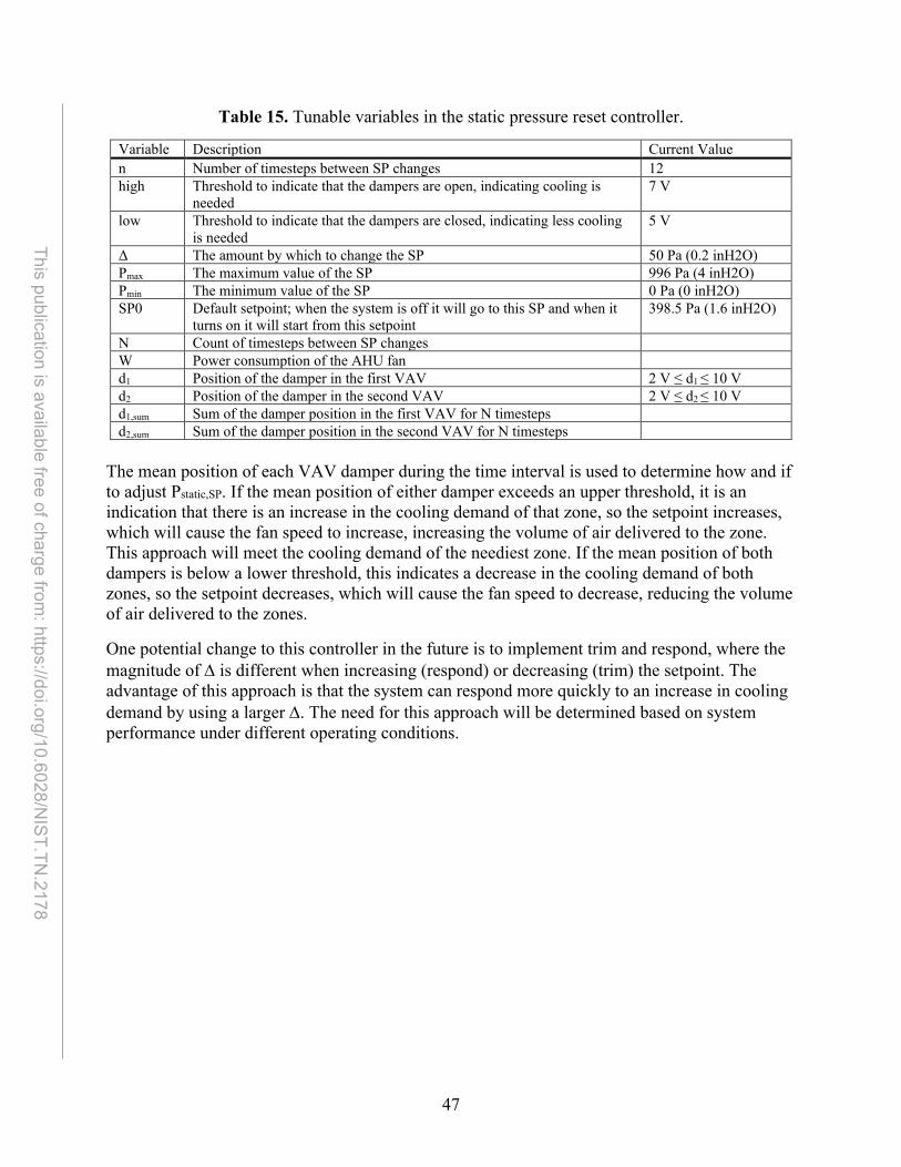
47


IST.TN.2178

Table 15. Tunable variables in the static pressure reset controller.

Variable Description Current Value n Number of timesteps between SP changes 12 high Threshold to indicate that the dampers are open, indicating cooling is

needed 7 V

low Threshold to indicate that the dampers are closed, indicating less cooling is needed

5 V

Δ The amount by which to change the SP 50 Pa (0.2 inH2O) Pmax The maximum value of the SP 996 Pa (4 inH2O) Pmin The minimum value of the SP 0 Pa (0 inH2O) SP0 Default setpoint; when the system is off it will go to this SP and when it

turns on it will start from this setpoint 398.5 Pa (1.6 inH2O)

N Count of timesteps between SP changes W Power consumption of the AHU fan d1 Position of the damper in the first VAV 2 V ≤ d1 ≤ 10 V d2 Position of the damper in the second VAV 2 V ≤ d2 ≤ 10 V d1,sum Sum of the damper position in the first VAV for N timesteps d2,sum Sum of the damper position in the second VAV for N timesteps

The mean position of each VAV damper during the time interval is used to determine how and if to adjust Pstatic,SP. If the mean position of either damper exceeds an upper threshold, it is an indication that there is an increase in the cooling demand of that zone, so the setpoint increases, which will cause the fan speed to increase, increasing the volume of air delivered to the zone. This approach will meet the cooling demand of the neediest zone. If the mean position of both dampers is below a lower threshold, this indicates a decrease in the cooling demand of both zones, so the setpoint decreases, which will cause the fan speed to decrease, reducing the volume of air delivered to the zones.

One potential change to this controller in the future is to implement trim and respond, where the magnitude of ∆ is different when increasing (respond) or decreasing (trim) the setpoint. The advantage of this approach is that the system can respond more quickly to an increase in cooling demand by using a larger ∆. The need for this approach will be determined based on system performance under different operating conditions.

48


IST.TN.2178

Fig. 24. Pseudocode describing the static pressure reset logic.

AHU Static Pressure Reset: Determine the duct static pressure used to set the fan speed

ahuPR( ) first call: N = 0; d1,sum = 0; d2,sum = 0; Pstatic,SP = SP0 1: if W > 50 // the fan is on 2: N = N + 1 3: d1,sum= d1,sum + d1 // sum of the damper position in the first VAV 4: d2,sum = d2,sum + d2 // sum of the damper position in the second VAV 5: if N > n 6: if ((d1,sum /N) or (d2,sum /N)) > high // more air is needed 7: Pstatic,SP = Pstatic,SP + ∆ 8: else if ((d1,sum /N) and (d2,sum /N)) < low 9: Pstatic,SP = Pstatic,SP – ∆ 10: endif 11: N = 0 12: d1,sum = 0 13: d2,sum = 0 14: endif 15: return Pstatic,SP = max(min(Pstatic,SP,Pmax),Pmin)

49


IST.TN.2178

Hydronic System Controllers

As mentioned in Sec. 2.1, the hydronic system supplies chilled water to the cooling coils in the AHUs. The chiller controller is a supervisory level controller that determines which chiller is enabled and what the setpoint temperature should be; proprietary local controllers determine the details of the chiller’s operation once it is enabled. The ice thermal storage tank can be used to deliver chilled water instead of the chillers, in which case its local level controller is enabled to modulate the flow rate of liquid through the tank. The temperature of the liquid that enters the cooling coils is controlled by a local level bridge controller in the secondary loop, and the volume of the liquid flow is determined by a local level pump controller. As previously mentioned, the base control loop timestep is 10 s, and all control logic is implemented in a custom LabVIEW program.

5.1. Chiller Controller

The chillers are controlled through a staging logic. Staging up means turning a chiller on, staging down means turning a chiller off. The decision on whether to stage up or down is based on the building load. Table 16 contains the variables and parameters used in the control algorithm that determines when to turn the chillers on and off. The current controller uses the four states shown in the table. A fifth state, state = 3, could be added as a case when both chillers operate at the same time, but this type of operation can cause problems. For example, when both chillers are operating, both pumps are operating, and when pumps operate in parallel, they must produce the same head, which impacts the flow rate of each pump. This tends to cause the flow rates to drop near or below the minimum flow rate required by each chiller. The possible implementation of this fifth state requires further testing.

50


IST.TN.2178

Table 16. Variables and parameters used in the control logic for staging chillers on and off.

Variable Description Typical Value state Describes the operation

of the chillers –1: Chillers in fault 0: No chillers on 1: Chiller1 on 2: Chiller2 on

NA

trans Describes the transition between states

trans01: Flag indicating a move from state = 0 to state = 1 trans02: Flag indicating a move from state = 0 to state = 2 trans12: Flag indicating a move from state = 1 to state = 2 trans21: Flag indicating a move from state = 2 to state = 1

NA

n Count the number of times a condition is violated; used to determine when to allow the state to change

n01: When state = 0, the number of counts when the building load exceeds q1_min n02: When state = 0, the number of counts when the building load exceeds q2_min n10: When state = 1, the number of counts when the building load is less than q1_sd n12: When state = 1, the number of counts when the building load exceeds q2_min n21: When state = 2, the number of counts when the building load is less than q2_sd

NA

N Count of the timesteps in transition NA n_trans Number of timesteps a transition lasts 27 n_viol Number of timesteps before which a state can change 10 q_min Minimum building load

required to turn on a chiller

q1_min: Minimum load to enable Chiller1 q2_min: Minimum load to enable Chiller2

q1_min: 3 kW q2_min: 25 kw

q_sd Building load at which a chiller is staged down

q1_sd: Load at which Chiller1 is staged down q2_sd: Load at which Chiller2 is staged down

q1_sd: 2 kW q2_sd: 23 kw

n_q_mean Number of timesteps over which the average load is calculated 3

When a state changes, for example from state = 1 to state = 2, the system does not instantaneously respond. The proprietary onboard chiller controller turns Chiller2 on at 17 % capacity for 180 s, then the chiller capacity ramps up as dictated by the controller and the system needs. If Chiller1 turns off as soon as the state changes from 1 to 2, there will be a period when Chiller2 is on, but at such a low capacity that the temperature in the system will increase above the setpoint, typically by several degrees. For this reason, transition actions are defined for

51


IST.TN.2178

moving between states. In this scenario, the transition action is noted by setting the variable trans12 = 1; during a transition, no other actions can be taken. A transition counter, N, increments during each timestep of the transition. When N exceeds n_trans, state = 2 and Chiller1 turns off while Chiller2, now ready to ramp up its capacity, meets the building load. The other variables in the table relate to how the algorithm decides what the state should be. The decision is based on the building load and how long the load has been at a given level. The behavior is best explained through an example. Take a scenario when the system is currently in state = 0, which means no chiller is operating. The building load begins to increase above q1_min, so the counter n01 increments. When n01 is greater than n_viol (i.e., the number of timesteps that violate the load threshold), trans01 = 1 and the transition from state = 0 to state = 1 begins. Chiller1 is enabled at that point and no further changes to the system can be considered until N > n_trans. Imagine that the building load continues to increase and is now greater than q2_min for n12 > n_viol; Chiller2 turns on and trans12 = 1. When N > n_trans, state = 2 and Chiller1 turns off. Note that all timers are reset once a transition is complete or a state changes. The key driver of the transitions is the building load, which can be calculated in several different ways:

• q_sl – based on the total temperature change across the secondary loop; • q_sl_sum – based on the sum of the loads on the water–side of the individual components

(cooling coils, heat exchanger) in the secondary loop; • q_air_sum – based on the sum of the loads on the air–side of the cooling coils plus the

load across HX1; • q_air_sum_sp – sum of the loads on the air–side of the cooling coil, where the

temperature at the outlet of the cooling coil is the setpoint temperature, plus the load across HX1.

All these quantities are calculated, and the maximum value is used as the estimate of the building load as a worst–case scenario. In theory, all but q_air_sum_sp should produce the same result, but there are uncertainties in the measurements and sometimes there are errors in a liquid flow rate measurement if there is too much air in the system, so looking at all possible calculations ensures there is always a reasonable estimate of the load. In addition, when the system is starting up the calculation of building load can be misleading.

Take a case where there is a call for cooling because of a load in the zone simulator. The AHU supply air setpoint is 12.8 °C (55 °F); the inlet temperature is 21.1 °C (70 °F) and the outlet temperature is 24 °C (75 °F). The cooling coil valve opens to allow flow through the coil and the fan is on. The load could be less than q1_min because the temperature change across the coil (DT) on both the PG and air–side is small. As the air warms up due to the ZS load, the DT could remain low, but maybe instead of the temperatures across the coil being 21.1 to 24 °C (70 to 75 °F), now they are 26.7 to 29.4 °C (80 to 85 °F). The key point is that the load will not cause the chiller to turn on; DT did not change, the airflow rate did not change, so the load is still below q1_min even though the air temperature is increasing. However, if a load is calculated based not on the actual air measurements of 21.1 to 24 °C, but the inlet air measurement of 21.1 °C and setpoint of 12.8 °C, q1_min can be large enough to cause Chiller1 to turn on.

52


IST.TN.2178

5.2. Bridge Temperature Controller

The secondary loop (SL) temperature, Tsl, is controlled by modulating mixing valve V9, which regulates the amount of return flow from the SL that mixes with supply flow from the PL (Fig. 25). The bridge shown in the figure hydraulically separates the PL from the SL, so the loops can have different flow rates, in addition to allowing for SL temperature control (see Sec. 1.6.3). Table 17 shows the current values of the PI parameters for SL valve control.

For example, take a case where the PL is operating to build ice in the thermal storage tank. The temperature of the PL is approximately –3.9 °C (25 °F) during this process. The SL is operating to meet a small building load, and the cooling coils need a temperature of 10 °C (50 °F). The PI control will set V9 at 4 V, so the 10 °C PG will be achieved by mixing 40 % cold PG with 60 % warmer PG returning from the cooling coils.

Fig. 25. PI loop for the SL valve position.

Kp

KI 1𝑠𝑠

Controller

+ – 𝑇𝑇𝑏𝑏𝑠𝑠,𝑆𝑆𝑆𝑆

𝑇𝑇𝑏𝑏𝑠𝑠

V9

bridge

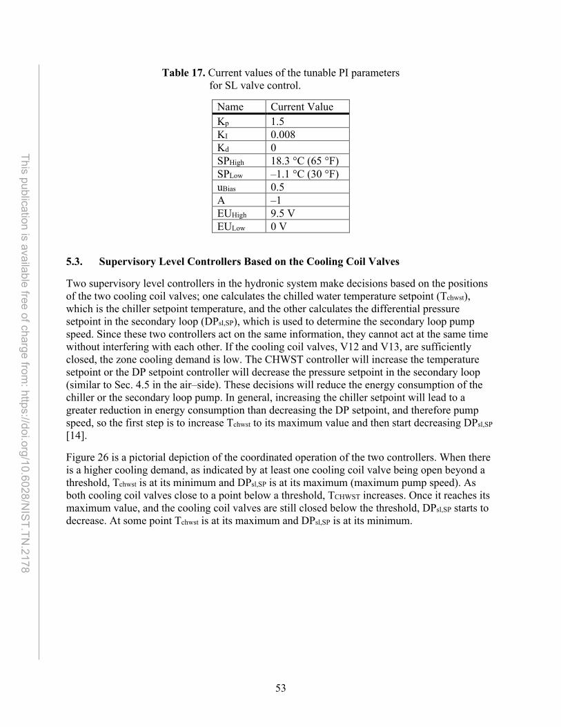
53


IST.TN.2178

Table 17. Current values of the tunable PI parameters for SL valve control.

Name Current Value Kp 1.5 KI 0.008 Kd 0 SPHigh 18.3 °C (65 °F) SPLow –1.1 °C (30 °F) uBias 0.5 A –1 EUHigh 9.5 V EULow 0 V

5.3. Supervisory Level Controllers Based on the Cooling Coil Valves

Two supervisory level controllers in the hydronic system make decisions based on the positions of the two cooling coil valves; one calculates the chilled water temperature setpoint (Tchwst), which is the chiller setpoint temperature, and the other calculates the differential pressure setpoint in the secondary loop (DPsl,SP), which is used to determine the secondary loop pump speed. Since these two controllers act on the same information, they cannot act at the same time without interfering with each other. If the cooling coil valves, V12 and V13, are sufficiently closed, the zone cooling demand is low. The CHWST controller will increase the temperature setpoint or the DP setpoint controller will decrease the pressure setpoint in the secondary loop (similar to Sec. 4.5 in the air–side). These decisions will reduce the energy consumption of the chiller or the secondary loop pump. In general, increasing the chiller setpoint will lead to a greater reduction in energy consumption than decreasing the DP setpoint, and therefore pump speed, so the first step is to increase Tchwst to its maximum value and then start decreasing DPsl,SP [14].

Figure 26 is a pictorial depiction of the coordinated operation of the two controllers. When there is a higher cooling demand, as indicated by at least one cooling coil valve being open beyond a threshold, Tchwst is at its minimum and DPsl,SP is at its maximum (maximum pump speed). As both cooling coil valves close to a point below a threshold, TCHWST increases. Once it reaches its maximum value, and the cooling coil valves are still closed below the threshold, DPsl,SP starts to decrease. At some point Tchwst is at its maximum and DPsl,SP is at its minimum.

54


IST.TN.2178

Fig. 26. Sketch of the coordinated operation of the secondary loop DP and CHWST controllers.

Figure 27 shows the pseudocode for determining if the mode is CHWST or DP. When the system first turns on, Tchwst = 10 °C (50 °F), which is between Tmax and Tmin, and DPsl,SP = DPmax. These points are show in Fig. 26 as a square and a triangle, respectively. So, when the system turns on it starts out in CHWST mode. Table 18 defines the variables used in this controller. The following sections describe the logic of each controller when in that mode.

Fig. 27. Pseudocode for determining if CHWST or DP controller is primary.

Tmax

Tmin

Tchwst DPsl,SP

higher cooling demand

lower cooling demand

DPmax

DPmin Secondary Loop Pressure Control

Chilled Water Setpoint Control

Mode Determination: Determine if the CHWST or DP controller should be enabled

mode( ) 1: if chMode == Auto and dpMode == Auto // both controllers are in auto

mode and the chiller and secondary loop pump are on

2: if Tchwst > Tmin and Tchwst < Tmax

3: mode = CHWST // the mode is CHWST 4: else 5: mode = DP // the mode is DP 6: endif 7: else if chMode == Auto and dpMode == Manual 8: mode = CHWST 9: else 10: mode = DP 11: end if 12: return mode

55


IST.TN.2178

Table 18. Variables used to determine the CHWST or DP mode.

Variable Description Current Value chMode Manual – manually set the chiller setpoint;

Auto – automatically set the chiller setpoint; requires that the chiller is on

Manual

dpMode Manual – manually set the secondary loop DP setpoint; Auto – automatically set the secondary loop DP setpoint; requires that the pump is on

Manual

Tchwst Current chiller setpoint NA Tmin Minimum chiller setpoint 4.4 °C (40 °F) Tmax Maximum chiller setpoint 21.1 °C (70 °F) mode CHWST – vary the chiller setpoint;

DP – vary the DP setpoint DP

5.3.1. CHWST

The calculation of Tchwst, is similar to the calculation of Pstatic,SP described in Sec. 4.5. Figure 28 shows the logic for calculating Tchwst and Table 19 defines the variables used in this calculation. Note that this controller is not used to determine the chiller setpoint when ice is being built in the thermal storage tank.

56


IST.TN.2178

Fig. 28. Pseudocode for calculating Tchwst.

Table 19. Variables in the CHWST controller.

Variable Description Current Value n Number of timesteps between SP changes 18 high Threshold to indicate that the valves are open, indicating more

cooling is needed 6 V

low Threshold to indicate that the valves are closed, indicating less cooling is needed

3.1 V

Δ The amount by which to change the SP 0.28 °C (0.5 °F) Tmin Minimum chiller setpoint 4.4 °C (40 °F) Tmax Maximum chiller setpoint 21.1 °C (70 °F) SP0 Default setpoint; when the system is off it will go to this SP and

when it turns on it will start from this setpoint 10 °C (50 °F)

N Count of timesteps between SP changes v12 Position of the valve in the cooling coil in AHU1 2 V ≤ v12 ≤ 10 V v13 Position of the valve in the cooling coil in AHU2 2 V ≤ v13 ≤ 10 V v12Sum Sum of the valve position in the cooling coil in AHU1 for N

timesteps

v13Sum Sum of the valve position in the cooling coil in AHU1 for N timesteps

W Chiller power consumption

Chilled Water Setpoint Temperature: Calculate the chiller setpoint temperature.

chwst( ) first call: N = 0; v12Sum = 0; v13Sum = 0; Tchwst = SP0 1: mode = mode() 2: if W > 100 and mode == CHWST // The chiller is on and the mode is

CHWST 3: N = N + 1 4: v12Sum = v12Sum + v12 // sum of the cooling coil valve position

in AHU1 during the N timesteps 5: v13Sum = v13Sum + v13 // sum of the cooling coil valve position

in AHU2 during the N timesteps 6: if N > n 7: if ((v12Sum/N) or (v13Sum/N)) > high // more cooling is

needed 8: Tchwst = Tchwst + ∆ 9: else if ((v12Sum /N) and (v13Sum /N)) < low 10: Tchwst = Tchwst – ∆ 11: endif 12: N = 0 13: v12Sum = 0 14: v13Sum = 0 15: endif 16: return Tchwst = max(min(Tchwst,Tmax),Tmin)

57


IST.TN.2178

There are some potential changes or expansions to the CHWST controller. For example, instead of using Tchwst as the chiller setpoint, it could be used as the setpoint for the primary loop or the secondary loop, and the chiller setpoint could be adjusted to achieve that setpoint. The advantage of this approach is that it could make it easier to use the thermal storage tank instead of the chillers, as well as to cope with the case when the chiller is being used to build ice in the thermal storage tank. As in the case of the static pressure reset controller in Sec. 4.5, it may also be better to implement a trim and respond approach so that the controller can react more quickly to an increase in cooling demand.

5.3.2. Secondary Loop Differential Pressure Reset

The calculation of DPsl,SP is similar to the calculation of Pstatic,SP described in Sec. 4.5. Figure 29 shows the location of the DP measurement in the secondary loop (DPsl) and Fig. 30 is the pseudocode for the determination of DPsl,SP. The variables in this controller are listed in Table 20. Note that in Fig. 29 the cooling coil valves, V12 and V13, are three–way mixing valves. In the current configuration of the IBAL, the manual valves in the horizontal bypass are closed, so V12 and V13 behave like two–way valves. This is a variable that can be investigated in the future.

Fig. 29. Location of the pressure drop measurement in the SL.

Cooling Coil

Cooling Coil

To/From Primary Loop

HX1

V10 V12 V13

DPsl

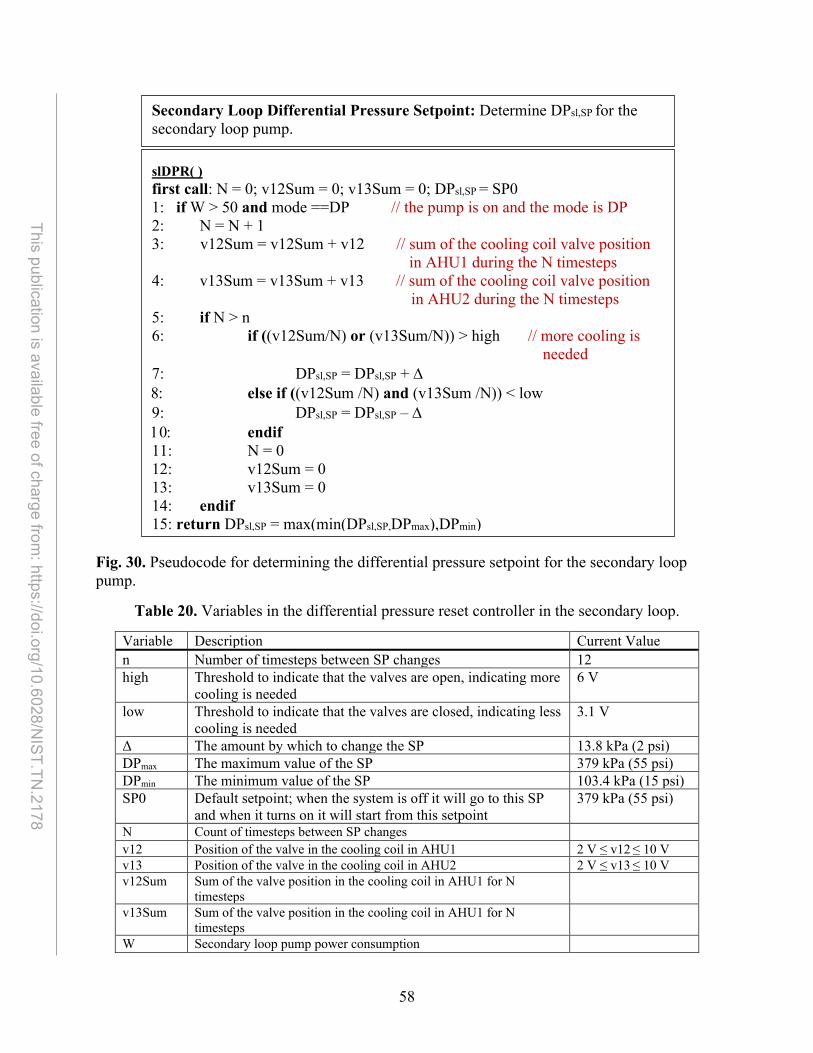
58


IST.TN.2178

Fig. 30. Pseudocode for determining the differential pressure setpoint for the secondary loop pump.

Table 20. Variables in the differential pressure reset controller in the secondary loop.

Variable Description Current Value n Number of timesteps between SP changes 12 high Threshold to indicate that the valves are open, indicating more

cooling is needed 6 V

low Threshold to indicate that the valves are closed, indicating less cooling is needed

3.1 V

Δ The amount by which to change the SP 13.8 kPa (2 psi) DPmax The maximum value of the SP 379 kPa (55 psi) DPmin The minimum value of the SP 103.4 kPa (15 psi) SP0 Default setpoint; when the system is off it will go to this SP

and when it turns on it will start from this setpoint 379 kPa (55 psi)

N Count of timesteps between SP changes v12 Position of the valve in the cooling coil in AHU1 2 V ≤ v12 ≤ 10 V v13 Position of the valve in the cooling coil in AHU2 2 V ≤ v13 ≤ 10 V v12Sum Sum of the valve position in the cooling coil in AHU1 for N

timesteps

v13Sum Sum of the valve position in the cooling coil in AHU1 for N timesteps

W Secondary loop pump power consumption

Secondary Loop Differential Pressure Setpoint: Determine DPsl,SP for the secondary loop pump.

slDPR( ) first call: N = 0; v12Sum = 0; v13Sum = 0; DPsl,SP = SP0 1: if W > 50 and mode ==DP // the pump is on and the mode is DP 2: N = N + 1 3: v12Sum = v12Sum + v12 // sum of the cooling coil valve position

in AHU1 during the N timesteps 4: v13Sum = v13Sum + v13 // sum of the cooling coil valve position

in AHU2 during the N timesteps 5: if N > n 6: if ((v12Sum/N) or (v13Sum/N)) > high // more cooling is

needed 7: DPsl,SP = DPsl,SP + ∆ 8: else if ((v12Sum /N) and (v13Sum /N)) < low 9: DPsl,SP = DPsl,SP – ∆ 10: endif 11: N = 0 12: v12Sum = 0 13: v13Sum = 0 14: endif 15: return DPsl,SP = max(min(DPsl,SP,DPmax),DPmin)

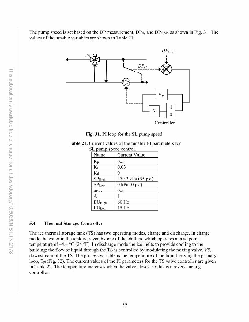
59


IST.TN.2178

The pump speed is set based on the DP measurement, DPsl, and DPsl,SP, as shown in Fig. 31. The values of the tunable variables are shown in Table 21.

Fig. 31. PI loop for the SL pump speed.

Table 21. Current values of the tunable PI parameters for SL pump speed control.

Name Current Value Kp 0.5 KI 0.03 Kd 0 SPHigh 379.2 kPa (55 psi) SPLow 0 kPa (0 psi) uBias 0.5 A 1 EUHigh 60 Hz EULow 15 Hz

5.4. Thermal Storage Controller

The ice thermal storage tank (TS) has two operating modes, charge and discharge. In charge mode the water in the tank is frozen by one of the chillers, which operates at a setpoint temperature of –4.4 °C (24 °F). In discharge mode the ice melts to provide cooling to the building; the flow of liquid through the TS is controlled by modulating the mixing valve, V8, downstream of the TS. The process variable is the temperature of the liquid leaving the primary loop, Tpl (Fig. 32). The current values of the PI parameters for the TS valve controller are given in Table 22. The temperature increases when the valve closes, so this is a reverse acting controller.

Kp

K

1𝑠𝑠

Controller

+ –

𝐷𝐷𝑆𝑆𝑏𝑏𝑠𝑠,𝑆𝑆𝑆𝑆

𝐷𝐷𝑆𝑆𝑏𝑏𝑠𝑠

V9

60


IST.TN.2178

Fig. 32. PI loop for the TS valve position.

Table 22. Current values of the tunable PI parameters for TS valve control.

Name Current Value Kp 0.1 KI 0.005 Kd 0 SPHigh 18.3 °C (65 °F) SPLow –1.1 °C (30 °F) uBias 0.5 A –1 EUHigh 9.5 V EULow 0 V

Kp

K

1𝑠𝑠

+ –

Controller

𝑇𝑇𝑝𝑝𝑠𝑠,𝑆𝑆𝑆𝑆 V8

Tpl

61


IST.TN.2178

Other Controllers in the IBAL

Several controllers have yet to be implemented in the IBAL. This section discusses the purpose of each controller and potential approaches for control. All these controllers are at the supervisory level and would benefit from an intelligent agent distributed optimization approach.

6.1. Secondary Loop Temperature Setpoint

The bridge controller (Secs. 1.6.3 and 5.2) is a local level controller that modulates a mixing valve to control the temperature of the liquid downstream of the secondary loop pump; this is the temperature of the liquid entering the cooling coils of the AHUs. Currently, the setpoint is manually set or is calculated as a constant offset from the chiller plant temperature setpoint. A supervisory level controller could consider factors such as the losses between the primary and secondary loops, the operating mode of the chiller plant (i.e., discharging the thermal storage, charging the thermal storage), and the building load.

6.2. Water–side Economizer Operation

Under certain conditions (low outdoor air wet–bulb temperature and low building load), a cooling tower can produce water that is cold enough to directly cool a building [15]. In other words, a chiller is not required to reduce the temperature of the tower water such that it can provide a sufficient heat sink for the building. This type of “free cooling” is achieved via a water–side economizer (WSE). In the IBAL, the WSE is a heat exchanger between the condensing loop and the primary loop that is plumbed in parallel with the chillers, so it can be used for cooling instead of a chiller. The preferred design is for the WSE to be plumbed in such a way that it can precool the water returning to the chiller, which allows increased efficiency of the chiller plant even when conditions do not allow for the WSE to meet the full building load, but constraints in the IBAL prevent this type of operation. In the future we will investigate different approaches for deciding when to use the WSE and how that decision can be made by an intelligent agent.

6.3. Air–side Economizer Operation

Under certain conditions, such as low outside air dry– and wet–bulb temperatures, the outdoor air can be directly used to cool the building with minimal or no additional conditioning; this is air–side economizer mode [16]. In the IBAL, air–side economizer mode can be enabled by changing the percent supply air setpoint, which changes the mixture of supply and return air. In normal operations, the supply and return dampers are positioned to provide the specified amount of ventilation air, typically based on local code requirements. The decision to operate in economizer mode is based on the temperature (or enthalpy) of the outside air and the supply air temperature setpoint, but an intelligent agent could be used to determine the optimal conditions for using the air–side economizer.

6.4. Primary Loop Flow Rate

In a typical primary secondary configuration for the hydronic system, the secondary loop has a variable flow rate and the primary loop has a fixed flow rate. In the IBAL there are three pumps plumbed in parallel in the primary loop. If Chiller1 is in use Pump1 is on, if Chiller2 is in use Pump2 is on, and if the WSE is in use Pump5 is on. Any of these pumps can be used with the ice

62


IST.TN.2178

thermal storage tank. Right now, when any of these pumps is on it is on at full speed (60 Hz), but each pump is operated by a variable frequency drive (VFD), so they can operate at lower speeds. There are some limitations on the pump speed because, for example, the chillers must receive a minimum required flow, but there is greater flexibility when, for example, the thermal storage is in discharge mode. The decision for setting the primary loop flow rate is based on factors including which equipment is in use, the temperature of the chiller plant output, and the building load. An intelligent agent approach would be very useful for this controller because of the broad scope of factors that contribute to the decision.

6.5. Condensing Loop Flow Rate

As in the case of the primary loop flow rate, the condensing loop flow rate is currently set by operating the pump, Pump4, at 60 Hz. Each chiller has an internal valve that determines the flow rate of water through the condenser via a proprietary controller. So, when a chiller is operating, the flow rate in the condensing loop could be set based on a differential pressure measurement; if the pressure increases (i.e., the chiller valve is closing), decrease pump speed. However, this does not address what the flow rate should be when using the WSE. A decision for that device would need to consider the load on the WSE, the temperature of the water delivered to the WSE, and the efficiency of the heat exchanger.

63


IST.TN.2178

Further Reading

Table 23 contains a list of resources for the reader interested in learning more about HVAC systems and controls. This is by no means a comprehensive list, but merely a starting point.

Table 23. Further reading.

Title Chapters 2019 ASHRAE Handbook of HVAC Applications [17]

Chapter 43: Supervisory Control Strategies and Optimization Chapter 48: Design and Application of Controls

2020 ASHRAE Handbook of HVAC Systems and Equipment [18]

Chapter 1: HVAC System Analysis and Selection Chapter 2: Decentralized Cooling and Heating Chapter 3: Central Cooling and Heating Plants Chapter 4: Air Handling and Distribution Chapter 23: Air–cooling and Dehumidifying Coils Chapter 43: Liquid–chilling Systems Chapter 50: Thermal Storage

2017 ASHRAE Handbook of Fundamentals [9]

Chapter 1: Psychrometrics Chapter 7: Fundamentals of Control

64


IST.TN.2178

References

[1] Pertzborn AJ, Veronica DA (2018) NIST Technical Note 2025: Intelligent Building Agents Laboratory: Air System Design. https://doi.org/10.6028/NIST.TN.2025

[2] Pertzborn AJ (2016) NIST Technical Note 1933: Intelligent Building Agents Laboratory: Hydronic System Design. https://doi.org/10.6028/NIST.TN.1933

[3] Thompson K (2021) Intelligent Buildings Agents Project. NIST. Available at https://www.nist.gov/el/energy–and–environment–division–73200/intelligent–buildings–agents–project

[4] Kelly GE, Bushby ST (2012) Are intelligent agents the key to optimizing building HVAC system performance? HVAC and R Research 18(4):750–759. https://doi.org/10.1080/10789669.2012.682693

[5] ASHRAE (1993) ASHRAE Air–Conditioning Systems Design Manual. (Atlanta, GA), RP–581.

[6] Altmann W, Macdonald D (2005) Practical Process Control for Engineers and Technicians (Elsevier).

[7] Seborg DE, Edgar TF, Mellichamp DA, Doyle III FJ (2016) Process Dynamics and Control (Wiley), 4th Ed.

[8] Wescott T (2000) PID Without a PhD. Embedded Systems Programming:86–108.

[9] ASHRAE (2017) 2017 ASHRAE Handbook of Fundamentals (ASHRAE, Atlanta, GA).

[10] Haines R, Wilson CL (1994) HVAC Systems Design Handbook (McGraw–Hill, New York, NY), 2nd Ed.

[11] Taylor ST, Stein J, Paliaga G, Cheng H (2012) Dual Maximum VAV Box Control Logic. ASHRAE Journal December 2012.

[12] Hydeman, Mark, Eubanks, Brent (2014) ASHRAE 1455–RP: Advanced Control Sequences for HVAC Systems – Phase I Air Distribution and Terminal Systems. ASHRAE Research Project Report. (ASHRAE), 1455–RP.

[13] Hydeman M, Taylor S, Stein J, Kolderup E, Hong T (2003) Advanced Variable Air Volume System Design Guide.

[14] Taylor S (2012) Optimizing Design & Control of Chilled Water Plants – Part 5: Optimized Control Sequences. ASHRAE Journal:56–74.

[15] ASHRAE (2020) Chapter 40: Cooling Towers. 2020 HVAC Systems and Equipment (ASHRAE, Atlanta, GA).

65


IST.TN.2178

[16] ASHRAE (2020) Chapter 4: Air Handling and Distribution. 2020 HVAC Systems and Equipment (ASHRAE, Atlanta, GA).

[17] ASHRAE (2019) 2019 ASHRAE Handbook of Applications (ASHRAE, Atlanta, GA).

[18] ASHRAE (2020) 2020 ASHRAE Handbook of HVAC Systems and Equipment (ASHRAE, Atlanta, GA).

Acknowledgments The authors thank the reviewers of this document, Steven Bushby, W. Vance Payne, John House, and David Yashar.

Documents

Baseline Control Systems in the Intelligent Building