BASELINE COMBINATION FOR INSAR DEM ATIMETRIC RESOLUTIONENHANCEMENT

Dominique Derauw(1) & Anne Orban(2)

(1)Centre Spatial de Liège, Avenue du Pré Aily, 4031 Angleur, Belgium, Email: dderauw@ulg.ac.be(2)Centre Spatial de Liège, Avenue du Pré Aily, 4031 Angleur, Belgium, Email : aorban@ulg.ac.be

ABSTRACT

Combination of several interferograms of a same area, each having its own ambiguity of altitude, allows producing acombined interferogram with either a better signal to noise ratio or a lower ambiguity of altitude, unreachable from asingle interferometric pair.

InSAR baseline combination by summation of interferograms allows reaching peculiar equivalent baselines whileincreasing signal to noise ratio in the resulting interferogram. Despite this drawback such combination revealed to behighly useful in atmospheric artifacts identification and localization. Choosing adequately the interferograms tocombine allow to generate interferograms with very short baseline in which the topographic phase component can beneglected, revealing artifacts before going further in a then useless processing.

Baseline combination by averaging can only be applied on unwrapped phases. Therefore, each interferogram must beunwrapped prior to combination. We thus implemented a three step phase unwrapping procedure allowing to take fullyadvantage of an interferometric data set containing several InSAR pairs of a given site. Phase averaging allows to lowersubstantially the phase standard deviation and thus to increase the altitude accuracy.

Baseline combination process was developed in the frame of an ESA DUP project [1] and of a TELSAT IV project [2].

1 BASELINE COMBINATION PROCESS DESCRIPTION

The phase in a single interferogram may be expressed as follow:

Dj+dlp

+p

+Dj=Dj ezn4

hha2

p (1)

Where:• the first term is the orbital phase term,• the second term is the topographical one, with ha the ambiguity of altitude,• the third term is the differential one, with ndz the optical path difference and n the refractive index,• the fourth term is the phase noise due to coherence losses between both considered wave fronts.

We consider here that there is no differential phase term. Moreover, interferograms are combined after flat earth phaseremoval. Therefore, only the second and fourth terms are to be considered in eq. 1.

1.1 Combination by addition

Two types of combination are possible. Either the interferograms are simply added or they are averaged. In case ofcombination by addition (or subtraction), the combined interferogram results in a phase expressed as:

eqeq

ii

ehha

2e

ha

1h2 Dj+

p=Dj+p=Dj   (2)

____________________________________________________________

Proc. of FRINGE 2003 Workshop, Frascati, Italy,1 – 5 December 2003 (ESA SP-550, June 2004) 31_derauw

The first type of combination allows to get very short equivalent ambiguity of altitude haeq but with increasing phase

noise, even if the signal to noise ratio is increased. Therefore, this first scheme may induce problems in the phaseunwrapping process. In the same way, combination by simple addition (or subtraction) allows to obtain combinedinterferograms having very high ambiguity of altitude. This can be very helpful when the fringe rate is to high to allowreliable phase unwrapping in order to obtain a "first order" topographic phase. As it will be shown hereafter, somecombination allows to generate interferograms having such a high equivalent ambiguity of altitude that no or fewtopographic phase is present. Such combinations are helpful for atmospheric artifact analysis.

1.2 Combination by averaging

Phases from independent interferograms can also be averaged. In this case, the resulting phase is:

  Dj+p=Dj ii

eN

1

ha

1

N

1h2 (3)

where N is the number of combined pairs. In this kind of combination, we can achieve an equivalent ambiguity ofaltitude with an averaged noise in the combined interferogram. The problem of averaging is that it is only applicable tounwrapped phase. Therefore, there is, a priori, no gain with respect to processing time nor with respect to noise induceddifficulties since each interferogram must be unwrapped independently.

1.3 Advantages versus drawbacks

From the foregoing, one may wonder what are the advantages of baseline combination since a priori; there is no gain inprocessing easiness. From one side, noise increases. On the other side, averaging can reduce noise but phaseunwrapping is needed for each interferograms.

In the next sections, we will see that, since we have several image pairs, a joint iterative phase unwrapping can beefficiently implemented. This joint phase unwrapping process allows us to obtain unwrapped phases better than thosethat can be independently generated. Therefore, baseline combination based on phase averaging keeps all its interest.

Secondly, as it will be shown hereafter, baseline combination by addition (or subtraction) is a powerful tool to show andstudy atmospheric artifacts.

2 TEST SITE AND DATA SET

Baseline combination process was implemented and validated on two distinct test sites: Brussels and Liège, Belgiumarea. These test sites offer a wide variety of land covers (urban, industrial, agricultural, forested,…) and landscape in alimited area. Moreover, a huge amount of ERS SAR data is available as well as exhaustive meteorological data and highresolution DEM to be used as reference for validation.

For the Brussels area, we have chosen to use only ERS1 data acquired during the "Second Ice Phase" of the ERS1mission (December 28, 1993 to April 9, 1994). This phase is characterized by a 3-day repeat cycle of acquisition abovea given point. For the Liège area, two sets of 5 ascending and descending Tandem ERS1-ERS2 InSAR pairs were used.As far as possible, winter tandem acquisitions were chosen.

Thanks to short lap between acquisitions, we can expect to keep a very good coherence between SAR scenes.Moreover, winter period ensures us to have a very low crop coverage and thus, to limit time decorrelation. Scenes wereselected after analysis of meteorological data. Concerning the Brussels test site, we have chosen 5 image pairs whosemain characteristics are given in table1.

Validation was performed by measuring and comparing phase standard deviation evolution with respect to the numberof combined interferograms as also by comparison with a high resolution provided by the National Geographic Institute(NGI) of Belgium (maximum error in height measurement of this reference is announced to be approximately 0.5 m).

table 1. Selected data setAcquisition orbit Interferométric baseline Ambiguity of

dates E1 E1 B// [m] B^ [m] altitude ha [m]

January 3, 1994 & December 31, 1993 12914 12871 41 111 -86February 5 &2, 1994 13387 13344 -46 -125 77

February 11 & 8, 1994 13473 13430 30 74 -130

February 17 & 14, 1994 13559 13516 -49 -134 -71

March 19 & 16, 1994 13989 13946 48 125 72

In order to ease nomenclature of the used scenes and generated interferometric products, we simply indexed the imageschronologically from 0 to 9. Therefore, as an example, i10 refers to interferogram made from the scenes acquired the 3rd

of January 1994 and the 31st of December 1993.

3 BASELINE COMBINATION FOR ATMOSPHERIC ARTIFACTS ANALYSIS

Looking to the altitude of ambiguity, we can deduce the usefulness of the following baseline combinations foratmospheric artifact analysis:

table 2. Useful baseline combination by addition for atmospheric artifact analysisi10 i32 i54 i76

i32 i32 + i10haeq > 730m

i54 3 * i54 - 2 * i10haeq > 5500m

2 * i54 + i32haeq > 400m

i76 i76 - i10haeq > 400m

i76 + i32haeq > 900m

i76 - 2 * i54haeq > 760m

i98 i98 + i10haeq > 440m

i98 - i32haeq > 1100m

i98 + 2 * i54haeq > 660m

i98 + i76haeq > 5000m

Knowing that the altitude of the covered area ranges between 0 and less than 250m, any of these combinedinterferograms must contain less than half a fringe. Moreover, some combinations have very large equivalent altitude ofambiguity. For these ones, the topographic phase must be nearly completely removed. The combined interferogramsmust show only the atmospheric component, baseline errors and local complex backscattering coefficient changes ifpresent.

All these combinations were tested and revealed that two pairs expected as good, contained in fact very importantatmospheric artifacts.

3.1 Example: interferogram combinations i76 – i10

Fig. 1. shows the interferogram combination obtained from i76 and i10. The equivalent altitude of ambiguity is of about400m. As a consequence, the topographical phase is not completely flattened but can only induce less than half of afringe in the south and less than a tenth of fringe in the north of the scene.

A vertical structure is clearly visible in the combination (fig. 1.). Since this structure is already visible in i76, it issuspected that this vertical structure is due to an atmospheric artifact contained in pair 76. It induces approximately aone-fringe step from left to right. It means that without this cross checking with other interferogram one may producecompletely erroneous DEM from this sole SAR pair with local height bias up to 70m.

Analysis of METEOSAT images showed nearly null cloud coverage for the 14 of February 1994 and a very low butapparently constant cloud cover for the 17th of February. This low cloud coverage seems sufficient to induce artifacts.Fig. 2. shows the METEOSAT images acquired the 17 of February 1994 at 21h30 and 22h00, thus 17 minutes beforeand 13 minutes after the SAR acquisition. When enhancing the contrast locally as shown in the figure, the cloud cover

appears less continuous. A straight cloud front appears in the north of Belgium having the same orientation than thestripes observed in the interferogram. As a consequence, it appears that the characteristics of the atmosphere shown bythe IR channel of METEOSAT have a strong influence on the phase in the generated SAR interferograms.

Fig. 1. interferograms i10, i76 and i76 – i10 interferogram combination

Fig. 2. Samples of METEOSAT IR images acquired just before and after the 17th February SAR acquisition

4 BASELINE COMBINATION BY AVERAGING

Baseline combination by averaging can only be applied on unwrapped phases. Therefore, each interferogram must beunwrapped prior to combination. The simplest scheme is to unwrap each phase up to residue connection. Havingconnection maps corresponding to each interferogram, one must superimpose them in order to have a commonconnection map to unwrap each interferogram. Finally, we obtain unwrapped phases sharing the same connections,allowing us to combine them by averaging. This simple and say, classical procedure is not very efficient.Superimposing the connection maps of each interferogram gives a common connection map containing all theconnection from each interferogram. There is thus no gain in the segmentation of the final combined phase. We thusimplemented a three step phase unwrapping procedure allowing to take fully advantage of an interferometric data setcontaining several InSAR pairs of a given site.

4.1 Three step phase unwrapping

From the analysis of the five SAR pairs of our data set, we chose the one that is the easiest to unwrap classically. Thispair is characterized by the highest mean coherence level in order to ensure to have a minimum number of residues tobe connected. The presence or absence of atmospheric artifact is not of prior importance since the aim is to obtain a firsttopographic phase approximation. On the other hand, the ambiguity of altitude must be chosen adequately because thisfirst topographic phase approximation must be retrieved from the other interferograms. Therefore, in a second step, thisphase shall be converted in the geometry of acquisition of each of the other pairs. This implies multiplication by factorsthat should be kept lower than 1 in order to avoid increasing the noise present in this first topographic phaseapproximation [3]. In our case, i10 corresponds to these characteristics. As an intermediate product during phaseunwrapping process, we generate a biased coherence used to guide the residue connection process. Since all the imagesare observing the same scene, this biased coherence is considered as representative as the one that might be obtained inall the pairs. In other words, we suppose that, even if the other pairs show lower coherence, the low coherence guides

should be mainly the same from one pair to another. After a classical phase unwrapping of i10 we obtain a firstapproximation of the topographic phase, which is then transposed in each of the acquisition geometry of each other pair.

The first topographic phase approximation is used to flatten each remaining interferograms. The flattenedinterferograms are then strongly filtered. For each interferogram, a residual phase term is then calculated as thedifference between the flattened interferogram and the filtered version of it. This residual phase term normally exhibitsphases distributed along a sharp peak centered on zero. If the distribution curve falls to zero outside the [-p/2, +p/2]interval, then this residual phase does not need to be unwrapped. Generally, the distribution does not fall to zero outsidethese bounds, but these phase levels are very few populated. Moreover, these phases correspond to areas having verylow coherence levels and for which, no valid topographic information can be obtained. Nevertheless, if the phasedistribution is too far from an ideal one falling to zero outside the interval [-p/2, +p/2], one must simply use a lessfiltered version of the flattened interferogram to generate the residual one. The phase unwrapping process is theninitiated on the filtered version of the flattened interferogram and stopped after the residues connections are generated.These connection maps show very few connections, since there are related to filtered and flattened interferograms.Next, all the connection maps are superimposed to get a common one that is used to unwrap each flattened and filteredinterferograms similarly. We thus obtain a second phase component for each interferogram

The third component of each unwrapped interferogram is given by the residual interferogram that does not need to beunwrapped as already explained.

Finally, each unwrapped phase is obtained by the summation of the three components. After this three-step phaseunwrapping, we obtain 5 topographic phases that can be averaged to generate the final DEM.

4.2 Advantages and drawbacks

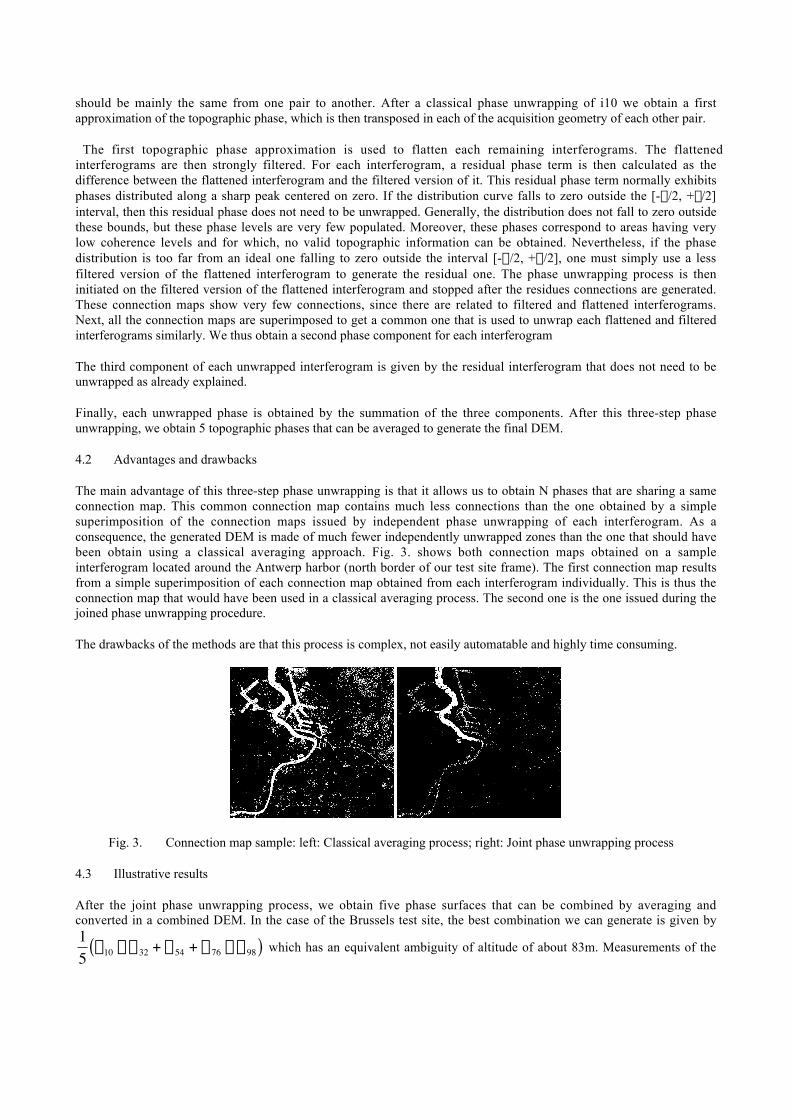
The main advantage of this three-step phase unwrapping is that it allows us to obtain N phases that are sharing a sameconnection map. This common connection map contains much less connections than the one obtained by a simplesuperimposition of the connection maps issued by independent phase unwrapping of each interferogram. As aconsequence, the generated DEM is made of much fewer independently unwrapped zones than the one that should havebeen obtain using a classical averaging approach. Fig. 3. shows both connection maps obtained on a sampleinterferogram located around the Antwerp harbor (north border of our test site frame). The first connection map resultsfrom a simple superimposition of each connection map obtained from each interferogram individually. This is thus theconnection map that would have been used in a classical averaging process. The second one is the one issued during thejoined phase unwrapping procedure.

The drawbacks of the methods are that this process is complex, not easily automatable and highly time consuming.

Fig. 3. Connection map sample: left: Classical averaging process; right: Joint phase unwrapping process

4.3 Illustrative results

After the joint phase unwrapping process, we obtain five phase surfaces that can be combined by averaging andconverted in a combined DEM. In the case of the Brussels test site, the best combination we can generate is given by

†

15

j10 - j32 + j54 + j76 - j98( ) which has an equivalent ambiguity of altitude of about 83m. Measurements of the

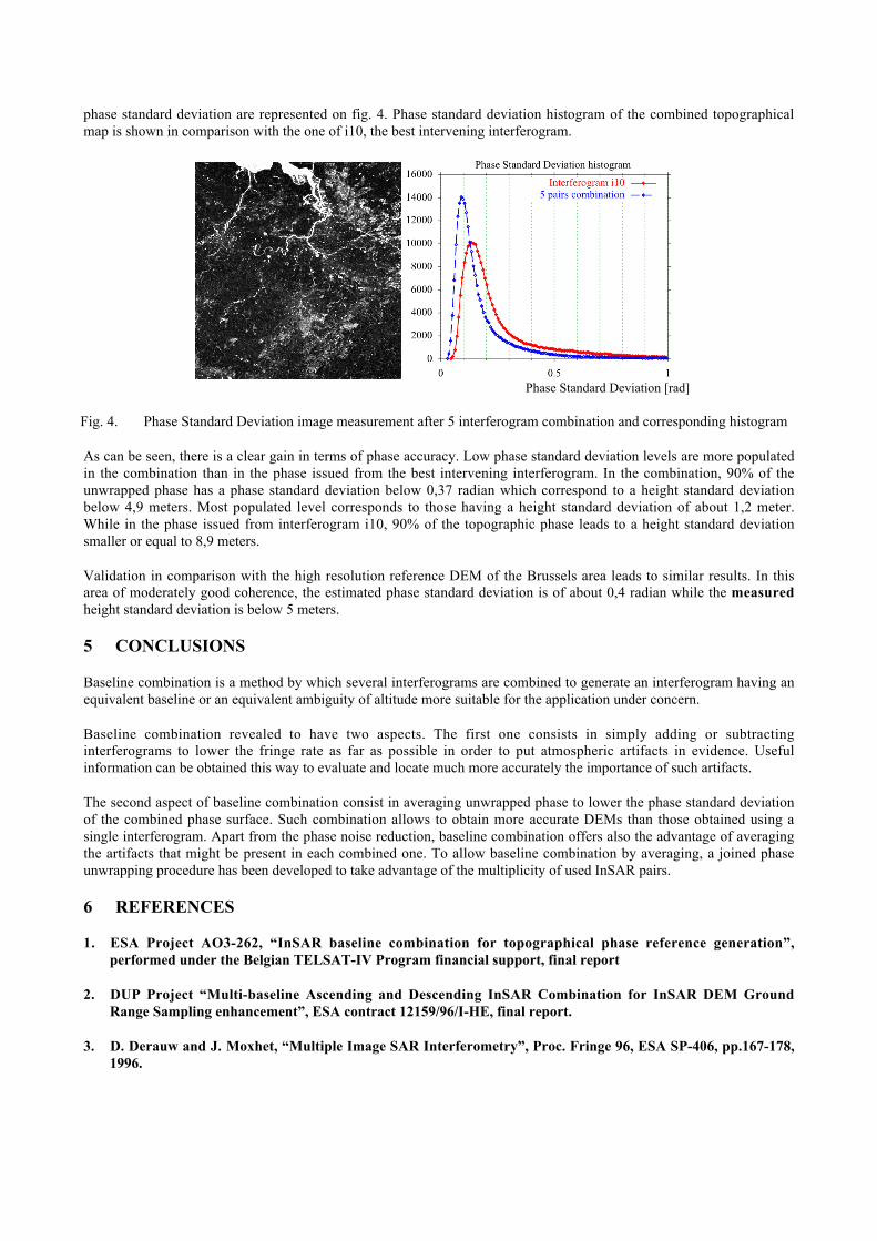
phase standard deviation are represented on fig. 4. Phase standard deviation histogram of the combined topographicalmap is shown in comparison with the one of i10, the best intervening interferogram.

Phase Standard Deviation [rad]

Fig. 4. Phase Standard Deviation image measurement after 5 interferogram combination and corresponding histogram

As can be seen, there is a clear gain in terms of phase accuracy. Low phase standard deviation levels are more populatedin the combination than in the phase issued from the best intervening interferogram. In the combination, 90% of theunwrapped phase has a phase standard deviation below 0,37 radian which correspond to a height standard deviationbelow 4,9 meters. Most populated level corresponds to those having a height standard deviation of about 1,2 meter.While in the phase issued from interferogram i10, 90% of the topographic phase leads to a height standard deviationsmaller or equal to 8,9 meters.

Validation in comparison with the high resolution reference DEM of the Brussels area leads to similar results. In thisarea of moderately good coherence, the estimated phase standard deviation is of about 0,4 radian while the measuredheight standard deviation is below 5 meters.

5 CONCLUSIONS

Baseline combination is a method by which several interferograms are combined to generate an interferogram having anequivalent baseline or an equivalent ambiguity of altitude more suitable for the application under concern.

Baseline combination revealed to have two aspects. The first one consists in simply adding or subtractinginterferograms to lower the fringe rate as far as possible in order to put atmospheric artifacts in evidence. Usefulinformation can be obtained this way to evaluate and locate much more accurately the importance of such artifacts.

The second aspect of baseline combination consist in averaging unwrapped phase to lower the phase standard deviationof the combined phase surface. Such combination allows to obtain more accurate DEMs than those obtained using asingle interferogram. Apart from the phase noise reduction, baseline combination offers also the advantage of averagingthe artifacts that might be present in each combined one. To allow baseline combination by averaging, a joined phaseunwrapping procedure has been developed to take advantage of the multiplicity of used InSAR pairs.

6 REFERENCES

1. ESA Project AO3-262, “InSAR baseline combination for topographical phase reference generation”,performed under the Belgian TELSAT-IV Program financial support, final report

2. DUP Project “Multi-baseline Ascending and Descending InSAR Combination for InSAR DEM GroundRange Sampling enhancement”, ESA contract 12159/96/I-HE, final report.

3. D. Derauw and J. Moxhet, “Multiple Image SAR Interferometry”, Proc. Fringe 96, ESA SP-406, pp.167-178,1996.