Embed Size (px)
Citation preview
Basel Committee on Banking Supervision
An assessment of the long-term economic impact of stronger capital and liquidity requirements
August 2010

Copies of publications are available from:
Bank for International Settlements Communications CH-4002 Basel, Switzerland
E-mail: [email protected]
Fax: +41 61 280 9100 and +41 61 280 8100
This publication is available on the BIS website (www.bis.org).
© Bank for International Settlements 2010. All rights reserved. Brief excerpts may be reproduced or translated provided the source is cited.
ISBN 92-9131-836-1 (print) ISBN 92-9197-836-1 (online)

An assessment of the long-term economic impact of the new regulatory framework
Contents
Executive summary ..................................................................................................................1
I. Introduction......................................................................................................................7
II. Economic benefits ...........................................................................................................8
II.A Benefits from reduced costs associated with banking crises .................................8
II.A.1 The frequency of banking crises.................................................................8
II.A.2 The economic costs of banking crises........................................................9
II.A.3 The expected benefits from reducing the frequency of banking crises ....12
II.A.4 The impact of capital and liquidity requirements on the probability of crises ....................................................................................................14
II.A.5. The impact of capital and liquidity requirements on the severity of crises ....................................................................................................17
II.B. Economic benefits from reducing the volatility of output ......................................18
III. Economic costs .............................................................................................................20
III.A. Changes in lending spreads.................................................................................21
III.A.1 The impact of higher capital requirements ...............................................21
III.A.2 Calculating the impact of higher liquidity requirements ............................23
III.B. Impact on the long-term steady-state level of output ...........................................25
IV. Net benefits ...................................................................................................................28
Annex 1: Costs of crises: a literature survey .........................................................................32
Annex 2: A brief summary of the crisis prediction/simulation models....................................41
Annex 3: Mapping higher capital and liquidity requirements to lending spreads ...................47
Annex 4: Description of the models used to assess the long-term cost of the new regulatory framework ......................................................................................53
Annex 5: Translating TCE/RWA into different bank capital ratios and modelling the link between the NSFR and banking crises ..................................................................56
Annex 6: Impact of tighter regulatory constraints on consumption ........................................59
References .............................................................................................................................60
Working group members ........................................................................................................63


An assessment of the long-term economic impact of the new regulatory framework 1
An assessment of the long-term economic impact of stronger capital and liquidity requirements
Executive summary
This report provides an analysis of the long-term economic impact (LEI) of the Basel Committee’s proposed capital and liquidity reforms.1 It assesses the economic benefits and costs of stronger capital and liquidity regulation in terms of their impact on output. The main benefits of a stronger financial system reflect a lower probability of banking crises and their associated output losses. Another benefit reflects a reduction in the amplitude of fluctuations in output during non-crisis periods. In this analysis, the costs are mainly related to the possibility that higher lending rates lead to a downward adjustment in the level of output while leaving its trend rate of growth unaffected. While empirical estimates of the costs and benefits are subject to uncertainty, the analysis suggests that in terms of the impact on output there is considerable room to tighten capital and liquidity requirements while still yielding positive net benefits.
In interpreting the findings of the report, two points are worth highlighting.
First, the report focuses on the long-run economic impact. The analysis assumes that banks have completed the transition to the new levels of capital and liquidity. To do this, it compares two steady states, one with and one without the proposed regulatory enhancements. The report does not assess the benefits and costs associated with the transition phase. The Macroeconomic Assessment Group (MAG) considers the macroeconomic costs of this transition, but not its benefits.2
Second, the report should not be viewed as indicating a particular calibration level. The Committee’s calibration is also being informed by its top-down assessment of the capital and liquidity frameworks and the results of the Quantitative Impact Study. Moreover, references to capital and liquidity ratios in this report are based on historical data and definitions and thus should not be read as corresponding directly to those proposed by the Basel Committee.3
Inevitably, the analysis of the macroeconomic benefits and costs is subject to considerable uncertainty. No single approach can capture all the implications of capital and liquidity regulation for bank behaviour and the economy at large. Thus, the report draws on a variety of methodologies and models. The presentation (including sensitivity analysis and technical annexes) provides a sense of the range of results across methodologies and potential uncertainties associated with the estimates.
1 This report was produced by the Basel Committee’s Long-term Economic Impact (LEI) working group, chaired
by Claudio Borio (BIS) and Thomas Huertas (UK FSA).
2 The MAG report is available at http://www.bis.org/publ/othp10.htm. 3 Throughout this report, capital is defined as tangible common equity (TCE) and the capital ratio as the ratio of
TCE to risk-weighted assets (RWA). TCE is net of goodwill and intangibles. RWA are measured using historical definitions under Basel I and Basel II. The analysis applies to total TCE held, so that it does not distinguish between the minimum capital requirement and additional capital that banks may hold in excess of the minimum requirement. The assessment of the liquidity regulations focuses on the Net Stable Funding Ratio (NSFR), as defined in the December 2009 proposal. At the same time, it also provides information pertinent to the assessment of the Liquidity Coverage Ratio (LCR).

2 An assessment of the long-term economic impact of the new regulatory framework
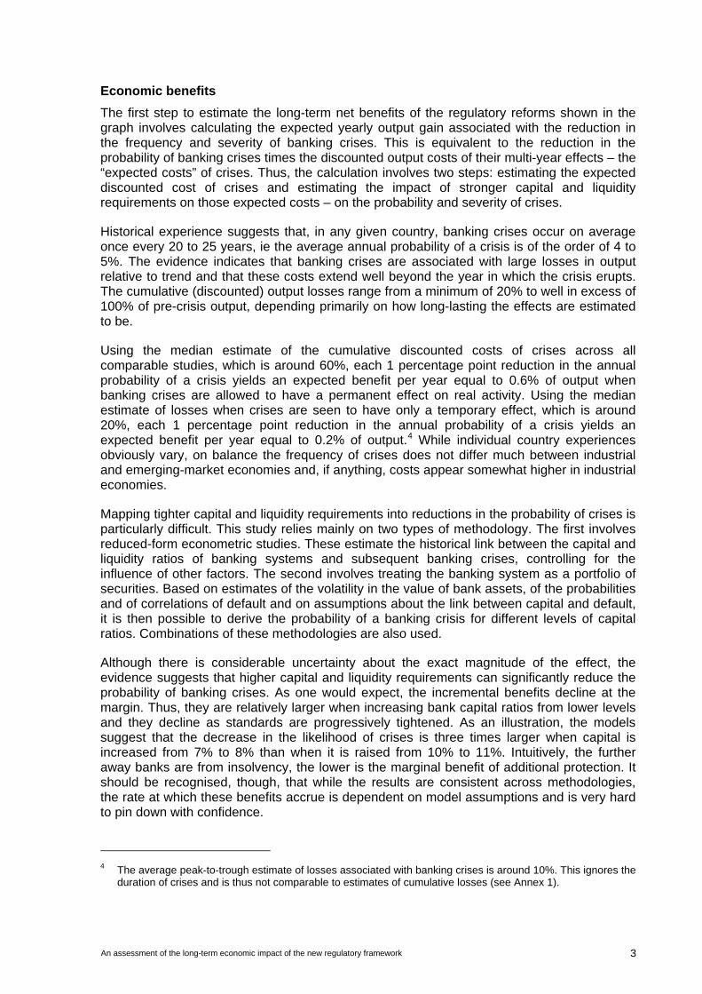
The core conclusions are illustrated in the graph below. The graph plots a range of estimates for the net benefits per year from reducing the probability of banking crises through higher capital standards while also meeting the liquidity requirements. The net benefits are measured in terms of the long-run change in the yearly level of output from its pre-reform path, with its trend growth rate unchanged. The origin corresponds to the historical average level of the capital ratio and frequency of banking crises – a proxy for the pre-reform steady state. The range of results shown reflects various estimates of the costs of banking crises, depending on whether costs are estimated as, permanent but moderate – which also corresponds to the median estimate across all comparable studies of such costs (red line) – or only temporary (green line). At the same time, taking a conservative approach, the results assume that institutions pass the added costs arising from strengthened regulations on to borrowers in their entirety while maintaining pre-reform levels for the return on equity, interest costs of liabilities and operating expenses. Thus, the costs of meeting the standards may be close to an upper bound.
Summary graph
Long-run expected annual net economic benefits of increases in capital and liquidity
Net benefits (vertical axis) are measured by the percentage impact on the level of output
Increasing capital and meeting liquidity requirements
Capital only
–0.5
0.0
0.5
1.0
1.5
2.0
2.5
8% 9% 10% 11% 12% 13% 14% 15% 16%Capital ratio
Moderate permanent effectsNo permanent effects
–0.5
0.0
0.5
1.0
1.5
2.0
2.5
8% 9% 10% 11% 12% 13% 14% 15% 16%Capital ratio
The capital ratio is defined as TCE over RWA. The origin corresponds to the pre-reform steady state, approximated by historical averages for total capital ratios (7%) and the average probability of banking crises. Net benefits are measured by the difference between expected benefits and expected costs. Expected benefits equal the reduction in the probability of crises times the corresponding output losses. The red and green lines refer to different estimates of net benefits, assuming that the effects of crises on output are permanent but moderate (which also corresponds to the median estimate across all comparable studies) or only transitory.
The core message of the graph is that net benefits remain positive for a broad range of capital ratios, with the incremental net benefits from reducing the probability of banking crises gradually declining to become negative beyond a certain range. Admittedly, the precise mapping between higher capital levels and stricter liquidity standards, on the one hand, and the reduction in the probability of crises, on the other, is quite uncertain. With this caveat, the sizeable gap between benefits and costs for a broad range of assumptions still suggests that in terms of the impact on output there is considerable room to tighten capital and liquidity requirements while still achieving positive net benefits.
The following presents in more detail the estimation methods, main results and broader set of factors that need to be considered when making an overall assessment. The body of the report provides detailed information on the dispersion of results and uncertainty surrounding them.
An assessment of the long-term economic impact of the new regulatory framework 3
Economic benefits
The first step to estimate the long-term net benefits of the regulatory reforms shown in the graph involves calculating the expected yearly output gain associated with the reduction in the frequency and severity of banking crises. This is equivalent to the reduction in the probability of banking crises times the discounted output costs of their multi-year effects – the “expected costs” of crises. Thus, the calculation involves two steps: estimating the expected discounted cost of crises and estimating the impact of stronger capital and liquidity requirements on those expected costs – on the probability and severity of crises.
Historical experience suggests that, in any given country, banking crises occur on average once every 20 to 25 years, ie the average annual probability of a crisis is of the order of 4 to 5%. The evidence indicates that banking crises are associated with large losses in output relative to trend and that these costs extend well beyond the year in which the crisis erupts. The cumulative (discounted) output losses range from a minimum of 20% to well in excess of 100% of pre-crisis output, depending primarily on how long-lasting the effects are estimated to be.
Using the median estimate of the cumulative discounted costs of crises across all comparable studies, which is around 60%, each 1 percentage point reduction in the annual probability of a crisis yields an expected benefit per year equal to 0.6% of output when banking crises are allowed to have a permanent effect on real activity. Using the median estimate of losses when crises are seen to have only a temporary effect, which is around 20%, each 1 percentage point reduction in the annual probability of a crisis yields an expected benefit per year equal to 0.2% of output.4 While individual country experiences obviously vary, on balance the frequency of crises does not differ much between industrial and emerging-market economies and, if anything, costs appear somewhat higher in industrial economies.
Mapping tighter capital and liquidity requirements into reductions in the probability of crises is particularly difficult. This study relies mainly on two types of methodology. The first involves reduced-form econometric studies. These estimate the historical link between the capital and liquidity ratios of banking systems and subsequent banking crises, controlling for the influence of other factors. The second involves treating the banking system as a portfolio of securities. Based on estimates of the volatility in the value of bank assets, of the probabilities and of correlations of default and on assumptions about the link between capital and default, it is then possible to derive the probability of a banking crisis for different levels of capital ratios. Combinations of these methodologies are also used.
Although there is considerable uncertainty about the exact magnitude of the effect, the evidence suggests that higher capital and liquidity requirements can significantly reduce the probability of banking crises. As one would expect, the incremental benefits decline at the margin. Thus, they are relatively larger when increasing bank capital ratios from lower levels and they decline as standards are progressively tightened. As an illustration, the models suggest that the decrease in the likelihood of crises is three times larger when capital is increased from 7% to 8% than when it is raised from 10% to 11%. Intuitively, the further away banks are from insolvency, the lower is the marginal benefit of additional protection. It should be recognised, though, that while the results are consistent across methodologies, the rate at which these benefits accrue is dependent on model assumptions and is very hard to pin down with confidence.
4 The average peak-to-trough estimate of losses associated with banking crises is around 10%. This ignores the
duration of crises and is thus not comparable to estimates of cumulative losses (see Annex 1).
4 An assessment of the long-term economic impact of the new regulatory framework
Intuitively, a stronger banking system should also be expected to reduce the severity of banking crises. Higher aggregate levels of capital and liquidity should help insulate stronger banks from the strains faced by weaker ones. There is, however, no extant research on this issue. The preliminary exploration carried out in this study, based on a simple reduced-form relationship akin to those used to estimate the impact on the probability of crises, finds some evidence of a relationship. However, the estimated relationship is statistically weak, perhaps owing to the limited number of observations that could be used (10 crises only). In the spirit of conservatism, the estimates are not used in the calculation of net benefits, effectively assuming that tougher standards have no impact on the severity of crises.
Economic costs
The long-run costs of higher capital and liquidity requirements on output are assessed using a variety of macroeconomic models, including a subset of those used by the MAG.5 The list includes dynamic structural general equilibrium (DSGE) models, semi-structural models and reduced-form models. In contrast to the MAG, because of the focus on the long-run steady state, higher capital and liquidity requirements are assumed to increase the cost of bank credit without additional non-price restrictions (eg credit rationing). The higher cost of bank credit lowers investment and consumption, in turn influencing the steady-state level of output.
The methodology to calculate the cost depends on the features of the macroeconomic models. In those that already include measures for capital and/or liquidity, changes in these variables can be imposed directly. In those that do not, it is first necessary to map regulatory requirements to lending spreads, or the cost of borrowing more generally, as this is always included in the models.
The mapping of changes in regulatory requirements into lending spreads relies on a representative bank’s balance sheet for several national banking systems. The pre-reform steady state is approximated by the average composition of the balance sheets over several years prior to the crisis, together with historical estimates of funding costs and returns on equity. Based on this, it is then possible to calculate the increase in lending spreads necessary to recover the additional costs of the higher standards. As already noted, this mapping is based on the conservative assumption that the whole adjustment is absorbed by lending rates, ie any increase in funding costs or reductions in returns on investments are fully passed through. It also assumes that the cost of capital does not fall as banks become less risky. It thus represents something closer to an upper bound.
This simple mapping yields two key results, with the central tendency across countries measured by the median estimate. First, each 1 percentage point increase in the capital ratio raises loan spreads by 13 basis points. Second, the additional cost of meeting the liquidity standard amounts to around 25 basis points in lending spreads when risk-weighted assets (RWA) are left unchanged; however, it drops to 14 basis points or less after taking account of the fall in RWA and the corresponding lower regulatory capital needs associated with the higher holdings of low-risk assets.
Not surprisingly, these results are sensitive to the return on equity (ROE) that banks are assumed to target. For example, if the average ROE is assumed to be 10% (rather than the 1993-2007 average of nearly 15% but consistent with a range of academic studies), then
5 A number of the models used by the MAG could not be employed because they do not have a well defined
steady state for the level of output, or this is difficult to compute. Even so, the results produced in this report are consistent with those produced by those models and the overall MAG results, when that steady state is approximated by the level of output at the end of the simulation period used by the MAG (eight years).
An assessment of the long-term economic impact of the new regulatory framework 5
each 1 percentage point increase in the capital ratio can be recovered by a 7 basis point rise in lending spreads.
Similarly, the results are very sensitive to the full-pass-through assumption. Banks have various options to adjust to changes in required capital and liquidity requirements other than increasing loan rates, including by reducing ROE, reducing operating expenses and increasing non-interest sources of income. Each of them could cut the costs of meeting the requirements. For example, on average across countries, a 4% reduction in operating expenses, or a 2 percentage point fall in ROE, is sufficient to absorb a 1 percentage point increase in the capital-to-RWA ratio. In practice, banks are likely to follow a combination of strategies.
Based on this intermediate step, it is then possible to estimate the impact of tougher regulatory requirements on output across the full set of macroeconomic models. A 1 percentage point increase in the capital ratio translates into a median 0.09% decline in the level of output relative to the baseline. The median impact of meeting the liquidity requirement is of a similar order of magnitude, at 0.08%.
Comparing benefits and costs – overall assessment
The various measures just described are then put together to quantify the net benefits shown in the summary graph. That graph indicates that, on balance, there is considerable scope to increase capital and liquidity standards while yielding positive net benefits. In reaching an overall assessment, however, it is important to highlight the factors that are not considered explicitly in the graph and that could make the final estimate of the net benefits higher or lower. Some of these factors have already been noted. In some cases, quantifying their effects is exceedingly difficult.
Several factors could lead to a higher estimate of net benefits:
In addition to reducing the probability of banking crises, higher capital and liquidity standards, by making the financial system more resilient, can reduce the amplitude of the business cycle. This impact can be enhanced through countercyclical capital buffer schemes. While hard to compare with the benefits included in the graph, these effects can be significant. They are evaluated in detail in section II.B and Annex 4 of this report.
In a similar way to that noted above, but focusing on crisis periods, a risk-averse society would be prepared to pay a premium over the expected costs of an extreme event such as a banking crisis (probability times its cost in terms of output) in order to insure against it, ie pay over the actuarially fair price. This premium has not been included in the calculations and would increase the benefits.
The expected costs of crises are based on data from historical episodes featuring large-scale government intervention to minimise the negative effects on output. In the absence of such intervention, the average costs of banking crises are likely to be significantly higher. In addition, the discount rate used to estimate the present value of the multi-year cost of crises is quite conservative.
To the extent that higher capital and liquidity requirements also reduce the severity of crises, the benefits will be higher.
The analysis assumes full pass-through of the higher funding costs/lower yield from investments to loan rates. However, in the long run it is reasonable to expect that, by reducing banks’ riskiness, higher capital and liquidity requirements should lead to lower debt and equity costs. Moreover, once adjustment is complete, differences
6 An assessment of the long-term economic impact of the new regulatory framework
between the cost of equity and debt could reduce to tax effects. Banks could also adjust by increasing efficiency or reducing operating expenses. These effects would substantially reduce the estimated long-run costs.
To the extent that greater intermediation is provided by the non-bank sector, the estimated costs will be lower.
Similarly, there are a number of factors that could reduce the net benefits:
The existing literature, which is the basis for this report’s estimates of the costs of banking crises, may overestimate the costs of banking crises. Possible reasons include: overestimation of the underlying growth path prior to the crises; failure to account for the temporarily higher growth during that phase; and failure to fully control for factors other than a banking crises per se that may contribute to output declines during the crisis and beyond, including a failure to accurately reflect causal relationships.
Capital and liquidity requirements may be less effective in reducing the probability of banking crises than suggested by the approaches used in the study. This would reduce the overall net benefits for a given level of the requirements. However, to the extent that net benefits remain positive, it would also imply that the requirements would need to be raised by more in order to achieve a given net benefit.
Shifting of risk into the non-regulated sector could reduce the financial stability benefits.
The results of the impact of regulatory requirements on lending spreads are based on aggregate balance sheets within individual countries, so that they do not consider the incidence of the requirements across institutions. They implicitly assume that the institutions that fall short of the requirements (ie, that are constrained) do not react more than those with excess capital or liquidity (ie, that are unconstrained). These effects may not be purely distributional.
As a final caveat, the results summarised above reflect the estimated net benefits associated with higher capital and liquidity standards, averaged across a number of countries over an extended period. Clearly, there is a range of uncertainty around estimates of central tendencies, reflecting data limitations and the need for various modelling assumptions. In addition, the estimated net benefits may be higher or lower in individual cases.
An assessment of the long-term economic impact of the new regulatory framework 7
I. Introduction
This report assesses the Long-term Economic Impact (LEI) of the Basel Committee’s December 2009 proposed reforms to the capital and liquidity frameworks. Its purpose is to assess the economic benefits and costs of more stringent capital and liquidity requirements once banks have completed the transition to the new requirements.
Importantly, the aim of the report is not to provide a specific calibration of the capital and liquidity requirements. Rather than gauging the optimal level of capital and liquidity requirements, the analysis aims at collecting and synthesising quantitative evidence regarding the relative magnitude of the macroeconomic benefits and costs. In doing so, it provides a range over which the benefits exceed the costs in the long run. Given the uncertainties involved in the assessment, this exercise simply helps to outline the contours for the calibration exercise. On balance, the analysis suggests that there is considerable room to tighten capital and liquidity requirements while still yielding positive net benefits, measured in terms of output.
The report focuses exclusively on the long run, or endpoint of the reforms. It assesses the shift from one steady state to another (with and without the reforms). As such, it does not assess the costs associated with the transition phase itself. The task of assessing the costs during the transition phase has been undertaken by the Macroeconomic Assessment Group (MAG).6 In addition, the MAG measures only costs. It does not consider the benefits that higher capital provides during the transition phase by making the banking system stronger. These benefits accrue immediately.
To interpret correctly the results of the report, the definition of capital is critical. Capital in this report refers to total capital holdings; no distinction is made between the minimum capital requirement and additional buffers. Moreover, capital is defined as tangible common equity (TCE)7 and the capital ratio as the ratio of TCE to risk-weighted assets (RWA), where RWA are based on definitions under Basel I and Basel II. The actual values of capital and RWA under the new proposals will therefore differ.8 In this context it must be stressed that the definitions used were in part dictated by the availability of data and, while related to regulatory ratios, they should not be read as exactly corresponding to either the Basel II ratios or the revised ratios under consideration by the Basel Committee.
The analysis of the impact of liquidity standards presents particular challenges. Under the BCBS’s December 2009 proposal, banks would be required to meet two new liquidity requirements – a short-term requirement called the Liquidity Coverage Ratio (LCR) and a long-term requirement called the Net Stable Funding Ratio (NSFR). The LCR ensures that banks have adequate funding liquidity to survive one month of stressed funding conditions. The NSFR addresses the mismatches between the maturity of a bank’s assets and that of its liabilities. The report focuses mainly on the NSFR, seen as the more relevant constraint for macroeconomic effects in the long run. In addition, data limitations made it especially hard to
6 The MAG was set up at the request of the Chairs of the BCBS and the FSB and is a collaborative effort
comprising representatives from central banks and regulators in 15 countries. The report of the MAG is available at http://www.bis.org/publ/othp10.htm.
7 Common equity = common stock + additional paid-in capital + retained earnings – treasury shares; tangible common equity = common equity – intangibles – goodwill.
8 Given that the models used to assess the economic benefits and costs are calibrated to a variety of historical capital adequacy measures, the analysis in this report uses a mapping from these measures to the ratio of TCE to RWA. This converts different ratios into a consistent variable using statistical techniques (see Annex 5).
8 An assessment of the long-term economic impact of the new regulatory framework
analyse the LCR for national banking systems. At the same time, the use of the ratio of liquid assets to total assets in specific parts of the analysis also provides information relevant for the assessment of the effects of the LCR. In this report, references to the liquidity requirement refer to the December 2009 proposal for the NSFR.
This report proceeds as follows. Section II outlines the steady-state economic benefits of stronger capital and liquidity requirements. The benefits reflect mainly a lower incidence of costly banking crises, but also a likely reduction in the amplitude of normal business cycles. Section III provides estimates of the steady-state economic costs of increasing capital and liquidity. Section IV brings together the analyses of the previous two sections to arrive at a range of quantitative estimates of those net benefits. It then highlights a set of factors not explicitly covered in the net benefit estimates and that should be taken into account when making an overall assessment. A series of annexes provide greater detail on the existing research into crises, on the models and methodologies used in this paper, and on the estimation results.
II. Economic benefits
The economic benefits of enhanced capital and liquidity regulations reflect mainly the fact that a more robust banking system would be less prone to crises that have large macroeconomic effects in terms of forgone output. Tighter regulatory standards may also lead to smaller output fluctuations and, hence, higher welfare even in the absence of banking crises. This section synthesises the evidence on these two effects. It first reviews the literature on the costs of banking crises and presents evidence on the impact of capital and liquidity regulation on the probability of systemic banking crises and on their severity. It then proceeds to discuss the evidence on the potential effect of tighter standards on the cyclical volatility of GDP.
The primary findings are: (i) on average, systemic banking crises have been very costly, with longer-term losses of output that are as high as multiples of annual GDP; (ii) better capitalisation and higher liquidity of banks reduce the likelihood of crises; (iii) there is some evidence that higher capital and liquidity reduce the severity of crises; and (iv) the reforms can reduce the amplitude of business cycles, not least if countercyclical capital buffers are in place.
II.A Benefits from reduced costs associated with banking crises
This report measures the expected yearly output gain associated with the reduction in the frequency and severity of banking crises as the reduction in the annual probability of banking crises times their output costs, ie as the reduction in the “expected costs” of crises. Linking stronger capital and liquidity requirements to the expected costs of crises requires estimation of the relationships of capital and liquidity ratios to the probability and severity of crises.
II.A.1 The frequency of banking crises
Averaging across countries and time, historical experience indicates that banking crises occur once every 20 to 25 years. The only period free of banking crises is that from the end of the Second World War until (depending on the country) the early 1970s–1980s – a period
An assessment of the long-term economic impact of the new regulatory framework 9
in which the financial sector was very heavily regulated.9 Crises have reoccurred and tended to become more frequent since then.
Table A1.4 in Annex 1 provides an overview of the banking crises in BCBS member countries since 1985. Different authors classify crises differently. Reinhart and Rogoff (2008) find 34 crises over the 25 year period, while Laeven and Valencia (2008) report only 24. Taking these together, it is possible to conclude that the frequency of crises ranges from 3.6% to 5.2% per year, with an average across samples and definitions of around 4.5%.10 Interestingly, the frequency of crises seems to be, if anything, slightly higher for G10 countries. In what follows, these average frequencies will be interpreted as the probability of a banking crisis in any given year and country.
II.A.2 The economic costs of banking crises
There is a substantial body of literature estimating the economic costs of banking crises in terms of GDP forgone. While researchers have adopted a variety of methods, on average the magnitude of the resulting GDP costs is estimated to be very large.
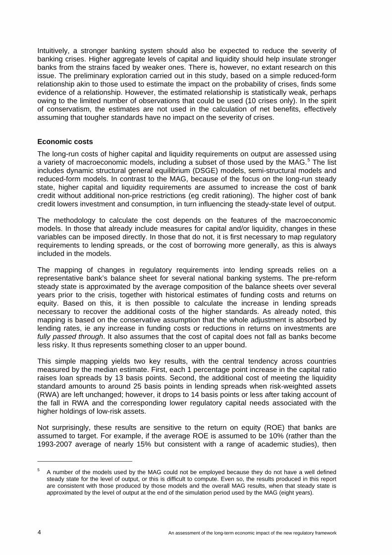
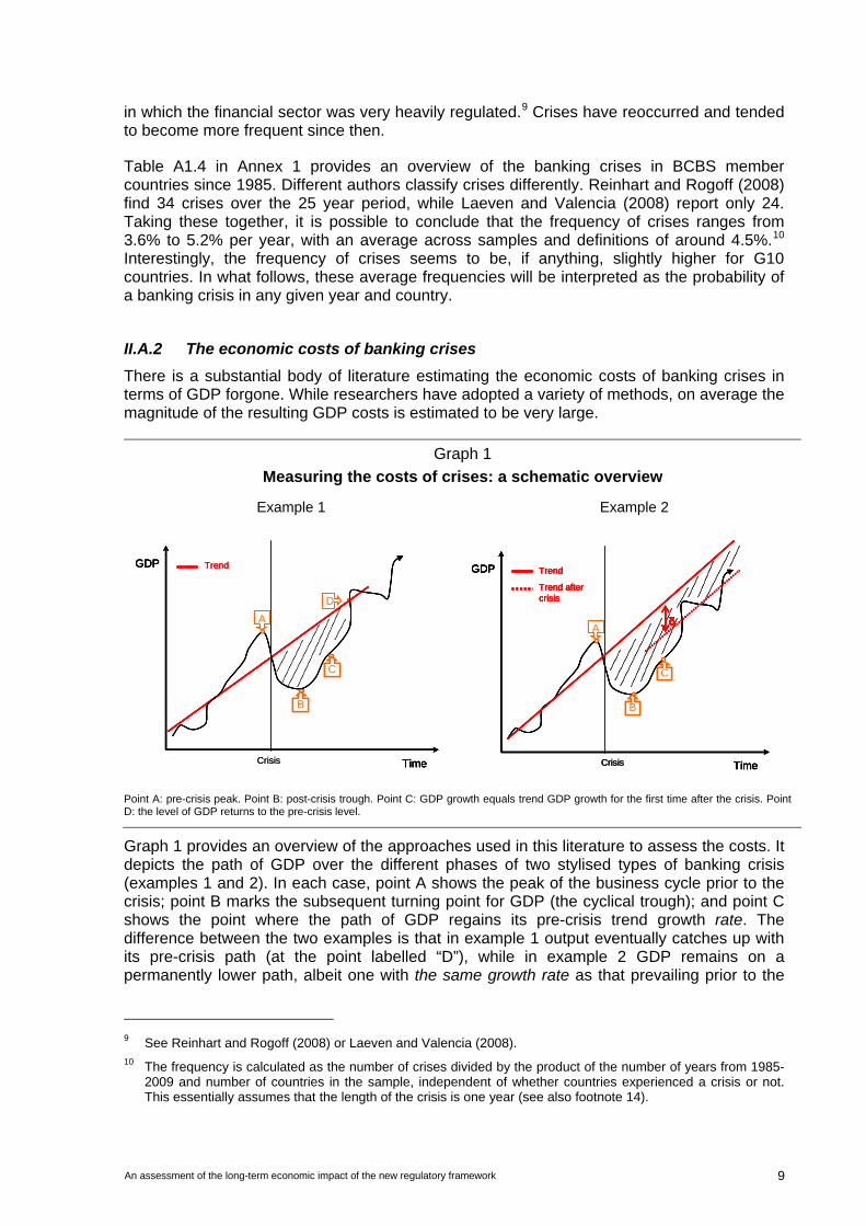
Graph 1
Measuring the costs of crises: a schematic overview
Example 1 Example 2
Point A: pre-crisis peak. Point B: post-crisis trough. Point C: GDP growth equals trend GDP growth for the first time after the crisis. Point D: the level of GDP returns to the pre-crisis level.
Graph 1 provides an overview of the approaches used in this literature to assess the costs. It depicts the path of GDP over the different phases of two stylised types of banking crisis (examples 1 and 2). In each case, point A shows the peak of the business cycle prior to the crisis; point B marks the subsequent turning point for GDP (the cyclical trough); and point C shows the point where the path of GDP regains its pre-crisis trend growth rate. The difference between the two examples is that in example 1 output eventually catches up with its pre-crisis path (at the point labelled “D”), while in example 2 GDP remains on a permanently lower path, albeit one with the same growth rate as that prevailing prior to the
9 See Reinhart and Rogoff (2008) or Laeven and Valencia (2008). 10 The frequency is calculated as the number of crises divided by the product of the number of years from 1985-
2009 and number of countries in the sample, independent of whether countries experienced a crisis or not. This essentially assumes that the length of the crisis is one year (see also footnote 14).
D
A
B
C
Time
GDP Trend
Crisis
D
A
B
C
Time
GDP Trend
A
B
C
Time
GDP
A
B
C
Time
GDP Trend
Crisis
A
B
C
Time
δ
GDP Trend
Trend after crisis
Crisis
A
B
C
Time
δ
GDP Trend
Trend after crisis
Crisis
A
B
C
Time
δ
GDP Trend
Trend after crisis
A
B
C
Time
δ
GDP
A
B
C
Time
δδ
GDP Trend
Trend after crisis
Crisis
10 An assessment of the long-term economic impact of the new regulatory framework
crisis. In example 2, the permanent loss in the level of GDP arising from the crisis is labelled δ. In other words, in example 1 the cost of the crisis is temporary, while in example 2 it is permanent.
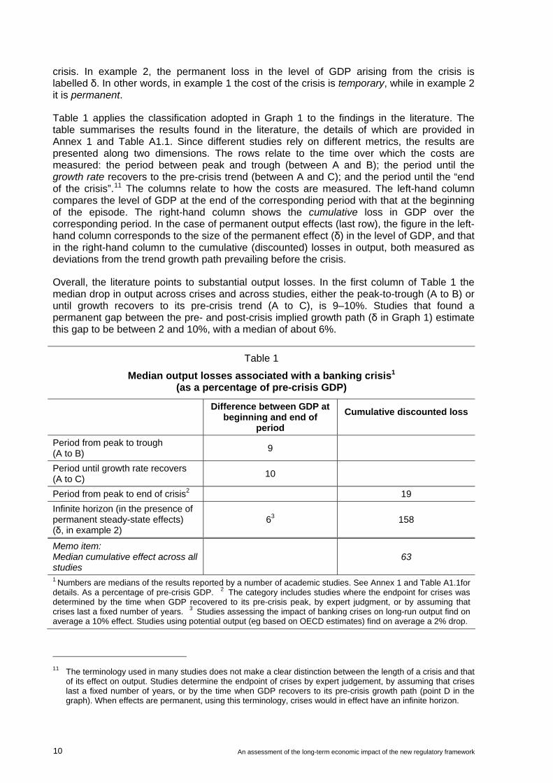
Table 1 applies the classification adopted in Graph 1 to the findings in the literature. The table summarises the results found in the literature, the details of which are provided in Annex 1 and Table A1.1. Since different studies rely on different metrics, the results are presented along two dimensions. The rows relate to the time over which the costs are measured: the period between peak and trough (between A and B); the period until the growth rate recovers to the pre-crisis trend (between A and C); and the period until the “end of the crisis”.11 The columns relate to how the costs are measured. The left-hand column compares the level of GDP at the end of the corresponding period with that at the beginning of the episode. The right-hand column shows the cumulative loss in GDP over the corresponding period. In the case of permanent output effects (last row), the figure in the left-hand column corresponds to the size of the permanent effect (δ) in the level of GDP, and that in the right-hand column to the cumulative (discounted) losses in output, both measured as deviations from the trend growth path prevailing before the crisis.
Overall, the literature points to substantial output losses. In the first column of Table 1 the median drop in output across crises and across studies, either the peak-to-trough (A to B) or until growth recovers to its pre-crisis trend (A to C), is 9–10%. Studies that found a permanent gap between the pre- and post-crisis implied growth path (δ in Graph 1) estimate this gap to be between 2 and 10%, with a median of about 6%.
Table 1
Median output losses associated with a banking crisis1
(as a percentage of pre-crisis GDP)
Difference between GDP at
beginning and end of period
Cumulative discounted loss
Period from peak to trough (A to B)
9
Period until growth rate recovers (A to C)
10
Period from peak to end of crisis2 19
Infinite horizon (in the presence of permanent steady-state effects) (δ, in example 2)
63 158
Memo item: Median cumulative effect across all studies
63
1 Numbers are medians of the results reported by a number of academic studies. See Annex 1 and Table A1.1for details. As a percentage of pre-crisis GDP. 2 The category includes studies where the endpoint for crises was determined by the time when GDP recovered to its pre-crisis peak, by expert judgment, or by assuming that crises last a fixed number of years. 3 Studies assessing the impact of banking crises on long-run output find on average a 10% effect. Studies using potential output (eg based on OECD estimates) find on average a 2% drop.
11 The terminology used in many studies does not make a clear distinction between the length of a crisis and that
of its effect on output. Studies determine the endpoint of crises by expert judgement, by assuming that crises last a fixed number of years, or by the time when GDP recovers to its pre-crisis growth path (point D in the graph). When effects are permanent, using this terminology, crises would in effect have an infinite horizon.
An assessment of the long-term economic impact of the new regulatory framework 11
Since all studies show that, even if temporary, the impact of banking crises lasts for several years, cumulative output losses are higher than peak-to-trough (A to B) declines. The median discounted cumulative loss of output over the course of a crisis estimated without allowing for the possibility of permanent effects (the area between the pre-crisis growth path and actual output between points A and D) is 19% of peak pre-crisis GDP (of point A). Studies that do allow for the possibility of permanent effects find them and estimate the corresponding median cumulative output loss at 158%. The median cumulative loss across all comparable studies is 63%.
These results from the existing literature are obviously based on crises prior to the current one. Haldane (2010) provides a range of estimates for the 2007–09 banking crisis assuming that a varying fraction of output losses experienced in 2009 will be permanent – the fractions are 25%, 50% and 100%. Using these figures, Haldane estimates that global output losses are a minimum of 90% of 2009 world GDP, but could rise to as high as 350% if the whole output loss turns out to be permanent (see Table A1.1).
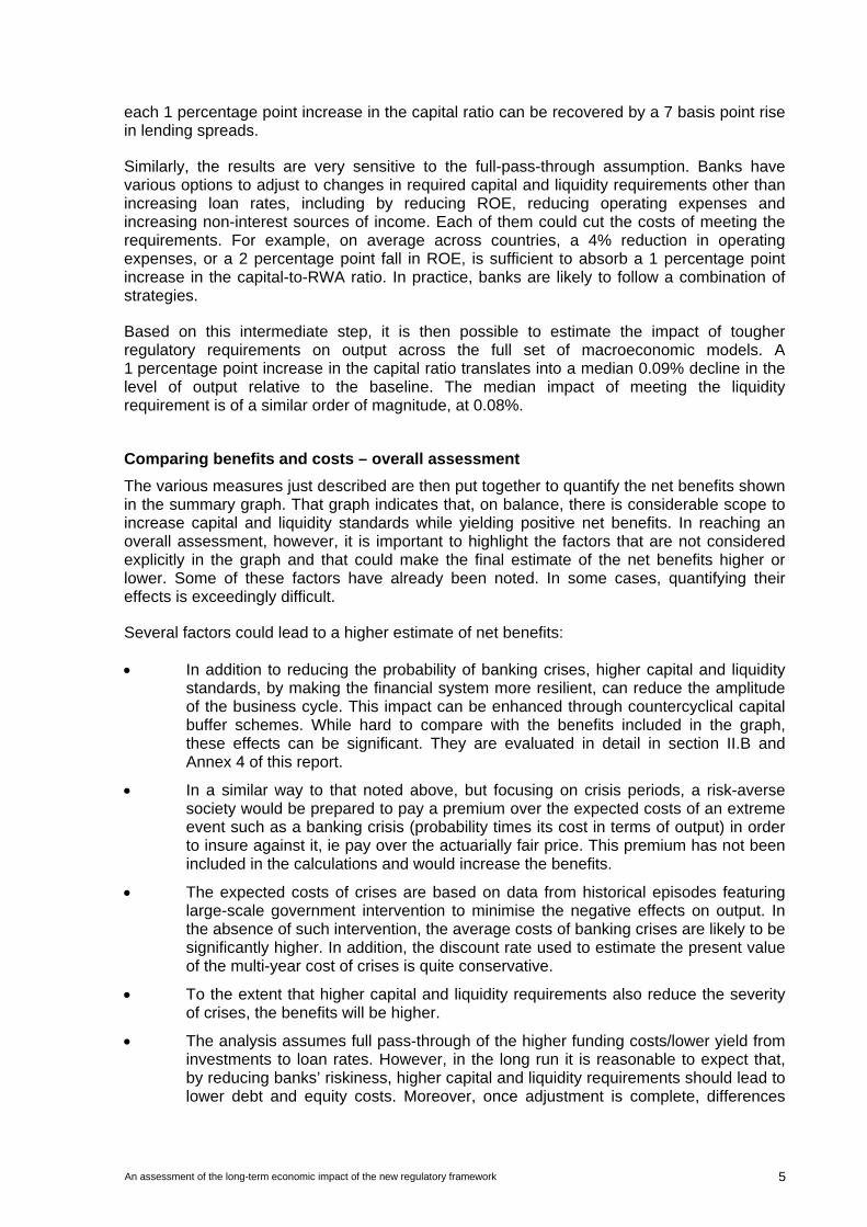
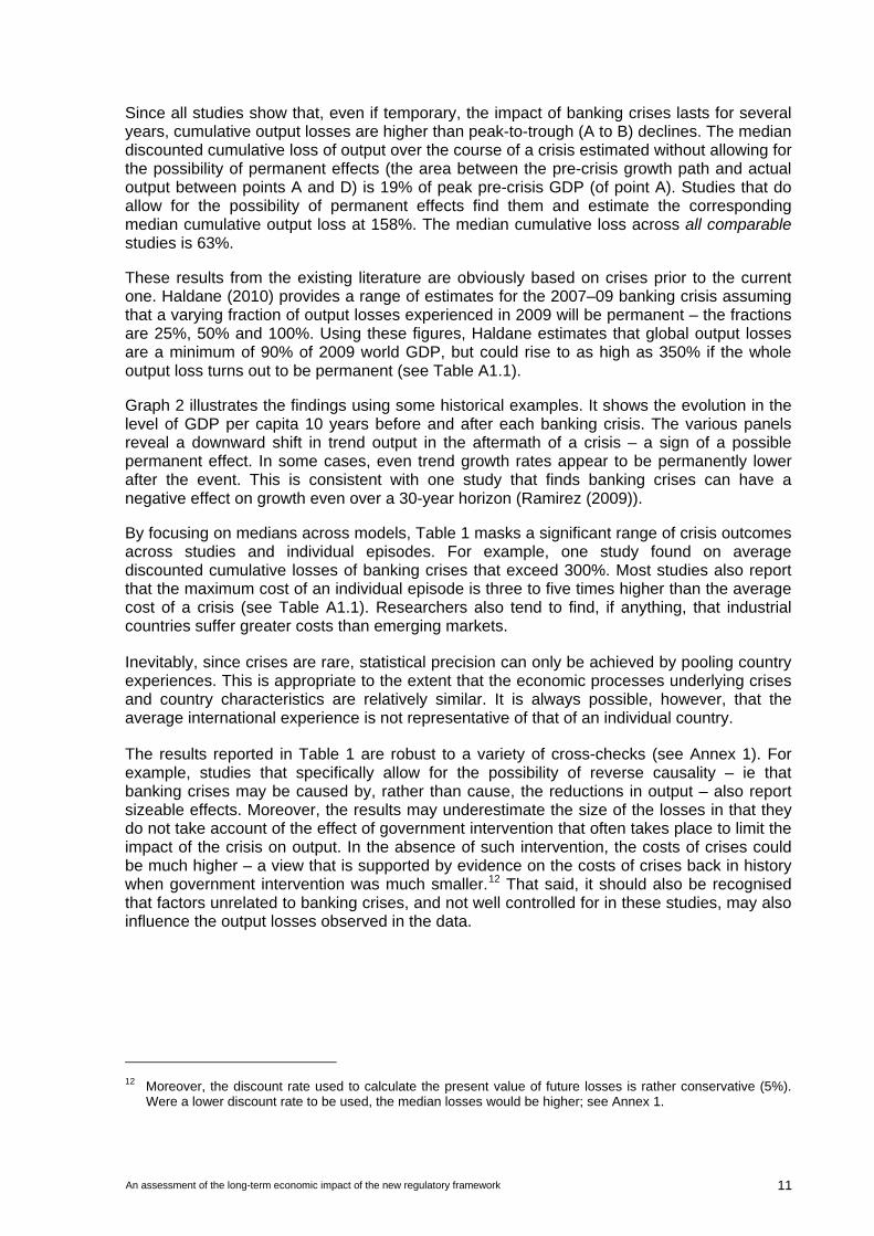
Graph 2 illustrates the findings using some historical examples. It shows the evolution in the level of GDP per capita 10 years before and after each banking crisis. The various panels reveal a downward shift in trend output in the aftermath of a crisis – a sign of a possible permanent effect. In some cases, even trend growth rates appear to be permanently lower after the event. This is consistent with one study that finds banking crises can have a negative effect on growth even over a 30-year horizon (Ramirez (2009)).
By focusing on medians across models, Table 1 masks a significant range of crisis outcomes across studies and individual episodes. For example, one study found on average discounted cumulative losses of banking crises that exceed 300%. Most studies also report that the maximum cost of an individual episode is three to five times higher than the average cost of a crisis (see Table A1.1). Researchers also tend to find, if anything, that industrial countries suffer greater costs than emerging markets.
Inevitably, since crises are rare, statistical precision can only be achieved by pooling country experiences. This is appropriate to the extent that the economic processes underlying crises and country characteristics are relatively similar. It is always possible, however, that the average international experience is not representative of that of an individual country.
The results reported in Table 1 are robust to a variety of cross-checks (see Annex 1). For example, studies that specifically allow for the possibility of reverse causality – ie that banking crises may be caused by, rather than cause, the reductions in output – also report sizeable effects. Moreover, the results may underestimate the size of the losses in that they do not take account of the effect of government intervention that often takes place to limit the impact of the crisis on output. In the absence of such intervention, the costs of crises could be much higher – a view that is supported by evidence on the costs of crises back in history when government intervention was much smaller.12 That said, it should also be recognised that factors unrelated to banking crises, and not well controlled for in these studies, may also influence the output losses observed in the data.
12 Moreover, the discount rate used to calculate the present value of future losses is rather conservative (5%).
Were a lower discount rate to be used, the median losses would be higher; see Annex 1.
12 An assessment of the long-term economic impact of the new regulatory framework
Graph 2
Output around banking crises
United States 2007 Japan 1992 United Kingdom 2007
0.96
0.98
1.00
1.02
1.04
99 01 03 05 07 09 11 13 15
Beginning of crisis2
Real GDP per capita1
Forecast
0.96
0.98
1.00
1.02
1.04
84 87 90 93 96 99 02
Beginning of crisis20.96
0.98
1.00
1.02
1.04
99 01 03 05 07 09 11 13 15
Beginning of crisis2
Mexico 1981 Korea 1997 Sweden 1991
0.96
0.98
1.00
1.02
1.04
73 76 79 82 85 88 91
Beginning of crisis2
0.96
0.98
1.00
1.02
1.04
89 92 95 98 01 04 07
Beginning of crisis20.96
0.98
1.00
1.02
1.04
83 86 89 92 95 98 01
Beginning of crisis2
1 GDP per capita is the logarithm of real GDP per capita, normalised to 1 at the beginning of the crisis. 2 The starting years for crisis are based on Laeven and Valencia (2008) and Reinhart and Rogoff (2008).
Source: IMF (2009).
Why should the effects of banking crises be so long-lasting, and possibly even permanent? One reason is that banking crises intensify the depth of recessions, leaving deeper scars than typical recessions. Possible reasons for why banking related crises are deeper include: a collapse in confidence; an increase in risk aversion; disruptions in financial intermediation (credit crunch, misallocation of credit); indirect effects associated with the impact on fiscal policy (increase in public sector debt and taxation); or a permanent loss of human capital during the slump (traditional hysteresis effects). To elaborate on this point, note that for output effects to be temporary, in the post-crisis period there needs to be an interval of above-trend growth that will return the economy to the path it would have followed in the absence of the crisis. As long as the channels listed above reduce potential output, there is no reason to expect a period of higher growth to follow after the adjustment has taken place. This may also hold in cases where the crisis is accompanied by a reduction in debt and the capital stock from unsustainable levels. During the stock adjustment phase, output growth is slower or negative until the excess is reabsorbed, at which point the economy can return to its previous trend growth rate. In such a case, the adjustment phase is not followed by a period of above average growth, so that permanent effects on output are observed.
II.A.3 The expected benefits from reducing the frequency of banking crises
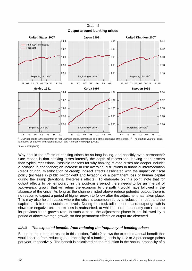
Based on the reported results in this section, Table 2 shows the expected annual benefit that would accrue from reducing the probability of a banking crisis by 1, 2 or 3 percentage points per year, respectively. The benefit is calculated as the reduction in the annual probability of a
An assessment of the long-term economic impact of the new regulatory framework 13
crisis times the cost of a crisis, measured as the discounted present value of the cumulative loss.
These benefits depend on the costs of the crisis. The first column reports the benefits arising under the assumption that crises have no permanent effects – the case in which the median cumulative loss is 19% of pre-crisis GDP ( = 0). The second column reports the benefits assuming the median cost of crises across all comparable approaches reported in the literature.13 This implies a loss equivalent to 63% of pre-crisis GDP and could be thought of as corresponding to a moderate permanent effect on output (eg = 3%). The third column looks at the consequences if the output costs of crises are assumed to be equal to the median loss reported by studies that allow for permanent effects (ie 158% of pre-crisis GDP or = 7.5%). However, given the uncertainty associated with the estimates and taking a prudent approach, less emphasis is placed on these results in the analysis that follows.14
The table shows that reducing the probability of crises has substantial benefits. Even in the absence of any permanent crisis-related output effects, a 1 percentage point reduction in the probability of crises generates a benefit on the order of 0.2% of GDP per year. When crises have long-lasting effects, the gains are commensurately larger, between 0.6% and 1.6% of GDP per year.
Table 2
Expected annual benefits of reducing the annual probability of crises1
Reduction in probability of crises (in percentage points)
Crises have no permanent effect
on output
Crises have a long-lasting or
small permanent effect on output
Crises have a large permanent effect on
output
1 0.19 0.63 1.58
2 0.38 1.26 3.16
3 0.57 1.89 4.74 1 The expected annual benefits are measured as the reduction in the annual probability of a crisis times the (discounted) cumulative output losses due to a banking crisis. Cumulative output losses are 19% (no permanent effect), 63% (small permanent or long-lasting) and 158% (large permanent). All the figures are in percentages of long-run GDP per year.
The results in Table 2 are simply the product of the change in the annual probability of a crisis and the cost if the crisis occurs. Put differently, these estimates do not depend on how the reduction in the likelihood of a crisis is achieved. The next section links the tighter regulatory standards to the change in the probability of a banking crisis.
13 This has to exclude the studies that measure output losses only as the peak-to-trough fall in GDP, as they do
not take into account the length of the crises (cumulative losses). 14 The high-side estimates are based on studies that extrapolate a significant portion of the observed post-crisis
shortfall in output into the indefinite future. However, the longer lasting the reduction in output, the greater the chance that it could reflect other factors, such as a persistent slowdown in trend productivity growth that occurred independently of the financial crisis; in fact, such factors may be an underlying cause of the financial crisis itself. Given this risk, it seems prudent to take a conservative approach and focus on the two lower sets of estimates in this analysis.

14 An assessment of the long-term economic impact of the new regulatory framework
II.A.4 The impact of capital and liquidity requirements on the probability of crises
The report uses three different methods to estimate the relationship between regulatory requirements and the probability of a crisis occurring in a given year: reduced-form models, calibrated portfolio models and calibrated stress test models. The results point to a clear role for capital. Liquidity is also important, but because it presents more data and modelling challenges than capital its impact is addressed by fewer models and results vary more across models. The rest of this section outlines the methodologies followed and presents the main results. Annex 2 provides a more detailed description of the models and the individual results.15
Methodologies
Reduced-form models estimate the probability of crises based on the statistical relationship between the incidence of crisis episodes and aggregate data on banks’ leverage and liquidity, as well as other variables that serve as controls. The report used results from three such models examining the experience of a panel of countries over a period of nearly 30 years (1980–2008).16 These models incorporate the impact of liquidity on the probability of crises, albeit in the form of the ratio of liquid assets to total assets rather than the ratios specified in the December 2009 proposals of the Basel Committee. Two models also makes a distinction between liquidity on the asset and liability (funding) sides of the balance sheet, by introducing the ratio of deposits to total liabilities as an additional variable.
Portfolio models employ standard portfolio credit risk methodologies to quantify the impact of higher regulatory requirements on the probability of systemic crises by treating the system as a portfolio of banks – each bank being the analogue of a security in a portfolio. One model uses data for five UK banks, including information on counterparty credit risk in the interbank market. The other model analyses a system of more than 50 large global banks. Both models use information from market prices as key input parameters, such as default correlations, in deriving the likelihood of a systemic crisis. Given their structure, however, neither of these models can assess the impact of liquidity requirements. With this in mind, the model estimated on the sample of global banks was augmented by a reduced-form relationship between the probability of default of the banks in the portfolio and their capital and liquidity ratios in order to produce another set of results that is also applicable to liquidity ratios.
The final approach used in this exercise relies on the Bank of Canada’s stress testing framework. This methodology is based on the idea that the failure of a bank arises from either a macroeconomic shock or spillover effects from other distressed banks. Spillover effects arise either because of counterparty exposures in the interbank market or because of asset fire sales that affect the mark to market value of banks’ portfolios. In this context, a greater buffer of liquid assets can only be beneficial insofar as it helps the bank to avoid asset fire sales, which would otherwise lead to losses. The resilience of the system is measured in terms of its response to very severe macroeconomic shocks.
Results
Table 3 summarises the core results. These are reported as the average probabilities of a crisis implied by the various models for different levels of capitalisation. The two right-hand
15 Annex 2 also reports point estimates of the probability of a systemic banking crisis, which correspond to
various capital ratios and, where appropriate, liquidity buffers for the individual modelling approaches. 16 One model was estimated by the UK FSA/NIESR, and the other two by the Bank of Japan (see Annex 2).

An assessment of the long-term economic impact of the new regulatory framework 15
columns of the table also report the impact of meeting different levels of strengthened liquidity standards using the subset of models that can analyse the impact of liquidity.
The interpretation of the results is subject to two caveats, which highlight the uncertainty surrounding the findings. First, as with all econometric exercises, many estimates reported here are based on historical correlations between capital and liquidity levels, on the one hand, and the occurrence of crises, on the other. These backward-looking correlations may not accurately represent future relationships or causal links. That said, the more structural calibrated portfolio models should be more robust to this critique, though these models also rely upon assumptions regarding long-run relationships among variables. Second, the models used in this context rely more than other parts of the analysis on capitalisation and liquidity ratios that are different from the standard ones used across the report.17 Hence, the interpretation of the results requires as an intermediate step a mapping of the relevant regulatory variables into those used in the models.18 The need to make these conversions using statistical estimates introduces additional uncertainty about the estimates, which is more pronounced in the case of the liquidity ratios. In this context it should be noted that actual levels held by banks typically include buffers above the minimum.
Table 3
The impact of capital and liquidity on the probability of systemic banking crises
(In percent)
All models
Models unable to assess
changes in liquid assets
Models incorporating changes in liquid assets
TCE/RWA No change in liquid assets
No change in liquid assets
No change in liquid assets
Meeting NSFR
(NSFR = 1)1 NSFR = 1.122
6 7.2 8.7 5.8 4.8 2.7
7 4.6 5.1 4.1 3.3 1.8
8 3.0 3.1 2.8 2.3 1.2
9 1.9 1.9 2.0 1.6 0.9
10 1.4 1.3 1.5 1.2 0.7
11 1.0 0.9 1.1 0.9 0.5
12 0.7 0.6 0.8 0.7 0.4
13 0.5 0.5 0.6 0.5 0.3
14 0.4 0.4 0.5 0.4 0.2
15 0.3 0.3 0.3 0.3 0.2
# models 6 3 3 3 3 1 Meeting the NSFR is modelled as a 12.5% increase in the ratio of liquid assets over total assets. 2 The NSFR equals 1.12 if liquid assets increase by 50% for the average bank.
17 Nearly all of the results reported below are based on models calibrated to the ratio of total capital to total
assets rather than to that of TCE to RWA. Similarly, due to the lack of data, the analysis of the impact of higher liquidity was first conducted in terms of the ratio of liquid assets to total assets and then converted (approximately) to the ratios in the BCBS December 2009 proposals.
18 Annex 5 describes the mapping procedure.

16 An assessment of the long-term economic impact of the new regulatory framework
A consistent result across different models and methodologies is a significant reduction in the likelihood of a banking crisis at higher levels of capitalisation and liquidity for the banking system as a whole. This is true both for the models that focus only on capital (summary shown in third column from the left) and those that incorporate liquidity effects (summary shown in the fourth column). A TCE/RWA capital ratio of 7% is roughly equivalent to the average capital to total asset ratio of 5% and is associated with a probability of a systemic crisis of 4.6%, which is roughly equal to the historical average experience.19 As a result, one can think of the corresponding row and the columns that do not consider any increase in the liquidity ratio as reflecting the pre-reform steady state. Increasing the capital ratio from 7% to 8%, with no change in liquid assets, reduces the probability of a banking crisis by one third (eg from 4.6% to 3.0%). Looking at the models that incorporate changes in liquid assets, increasing the liquidity ratio to meet the NSFR while keeping a capital ratio of 7% reduces the likelihood of systemic banking crises from 4.1% to 3.3%. The reduction in the probability of crises continues as capital and liquidity levels increase, as can be seen by comparing figures down the rows (for capital) and across the three columns on the right-hand side (for liquidity). In fact, if the liquid assets to total assets ratio exceeds the proposed liquiidty requirement, at a 7% TCE/RWA ratio, the estimated reduction in the probability of crises is about the same as that associated with an increase of 2 percentage points in the capital ratio (from 7% to 9%).
Another consistent result across models is that the incremental benefit of higher capital and liquidity requirements declines as the system becomes better capitalised. That is, when banks have low levels of capital, even small increases have a very significant impact, but the marginal benefit of further increases in capital ratios declines as banks move further away from the insolvency threshold. For instance, increasing capitalisation from 10% to 11% induces a drop in the likelihood of crises about one quarter to one third of the corresponding estimated drop when TCE/RWA increased from 7% to 8%. Similarly, the incremental fall in crisis probabilities from a tightening of liquidity standards declines as the levels of capital increase. These results are fairly intuitive. The rationale is quite similar to that applying in the context of risk models applied to individual banks. For a given volatility in the value of assets, the further away a bank is from the insolvency threshold, the lower is the benefit of additional protection.
This declining marginal contribution of capital and liquidity in reducing the probability of crises has two important implications. First, the benefits of tighter standards are not without bounds but they plateau at some point. Second, the benefits will depend not only on the initial conditions for capital and liquidity, but also on the other conditioning variables used to calibrate these models.
As mentioned earlier, these results on the impact of tighter regulatory standards on the probability of crises are subject to considerable model and estimation uncertainty. Despite the fact that the message from different models is quite consistent, there is a possibility that the effect could be different from that estimated. One possibility is that the decline in the probability of crises is more gradual than suggested by Table 4 and Annex 2. If so, the rate at which benefits of tighter regulatory standards accrue would be lower than reported. This could arise, for instance, if banks responded in part to the imposition of standards by seeking to increase the risks they take on (eg, increase the volatility of their assets) in undetected ways. However, to the extent that net benefits remain positive, in order to achieve a comparable level of benefits, standards would have to be tightened further than implied by
19 The average ratio of total capital and reserves to total assets for the 14 largest OECD countries from 1980 to
2007 is 5.3%. Using an average of the conversion tables presented in Annex 5, a TCE/RWA ratio of 7% is equivalent to a 5% ratio of total shareholder equity over total assets.

An assessment of the long-term economic impact of the new regulatory framework 17
this analysis. In other words, the overall economic gain might be lower but capital and liquidity standards would have to be set at a higher level in order to bring about these benefits.
II.A.5. The impact of capital and liquidity requirements on the severity of crises
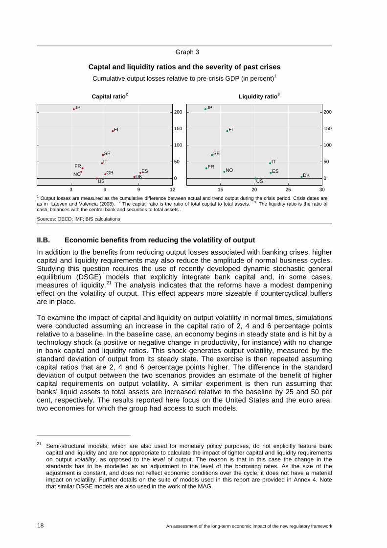
Higher capital and liquidity standards are likely to reduce not just the probability, but also the severity of banking crises. Intuitively, higher aggregate levels of capital and liquidity should help insulate stronger banks from the strains faced by the weaker ones. Surprisingly, there is no extant academic research on this issue. That said, a simple exploration of the data provides some support for this intuition.
Graph 3 is a scatter plot of the estimated GDP costs of crises (on the vertical axis) against the aggregate level of capital and liquidity buffers in each country’s banking system immediately prior to the onset of the crisis (on the horizontal axis). The data suggest that lower capital-to-asset ratios and lower liquidity ratios are associated with higher output losses during the ensuing crisis. Unfortunately, the relationship is relatively weak, with the implied regression coefficient not statistically different from zero – a result that may be due to the limited number of observations (10 crises only).20 In the spirit of conservatism, these possible benefits are not included in the calculation of net benefits discussed in section IV below, effectively assuming that tougher standards have no impact on the severity of crises.
20 Comparing capital and liquidity buffers with the length of systemic banking crises yields similar results. The
number of years that it takes for GDP to return to its long-run trend growth rate is inversely related to the aggregate level of the two types of buffers prior to the crisis. Statistics presented in Barrell et al (2010b) support this finding.
18 An assessment of the long-term economic impact of the new regulatory framework
Graph 3
Captal and liquidity ratios and the severity of past crises
Cumulative output losses relative to pre-crisis GDP (in percent)1
Capital ratio2 Liquidity ratio3
ES
FI
FRGB
IT
JP
NO
SE
USDK 0
50
100
150
200
3 6 9 12
ES
FI
FRIT
JP
NO
SE
USDK
0
50
100
150
200
15 20 25 301 Output losses are measured as the cumulative difference between actual and trend output during the crisis period. Crisis dates are as in Laeven and Valencia (2008). 2 The capital ratio is the ratio of total capital to total assets. 3 The liquidity ratio is the ratio of cash, balances with the central bank and securities to total assets .
Sources: OECD; IMF; BIS calculations
II.B. Economic benefits from reducing the volatility of output
In addition to the benefits from reducing output losses associated with banking crises, higher capital and liquidity requirements may also reduce the amplitude of normal business cycles. Studying this question requires the use of recently developed dynamic stochastic general equilibrium (DSGE) models that explicitly integrate bank capital and, in some cases, measures of liquidity.21 The analysis indicates that the reforms have a modest dampening effect on the volatility of output. This effect appears more sizeable if countercyclical buffers are in place.
To examine the impact of capital and liquidity on output volatility in normal times, simulations were conducted assuming an increase in the capital ratio of 2, 4 and 6 percentage points relative to a baseline. In the baseline case, an economy begins in steady state and is hit by a technology shock (a positive or negative change in productivity, for instance) with no change in bank capital and liquidity ratios. This shock generates output volatility, measured by the standard deviation of output from its steady state. The exercise is then repeated assuming capital ratios that are 2, 4 and 6 percentage points higher. The difference in the standard deviation of output between the two scenarios provides an estimate of the benefit of higher capital requirements on output volatility. A similar experiment is then run assuming that banks’ liquid assets to total assets are increased relative to the baseline by 25 and 50 per cent, respectively. The results reported here focus on the United States and the euro area, two economies for which the group had access to such models.
21 Semi-structural models, which are also used for monetary policy purposes, do not explicitly feature bank
capital and liquidity and are not appropriate to calculate the impact of tighter capital and liquidity requirements on output volatility, as opposed to the level of output. The reason is that in this case the change in the standards has to be modelled as an adjustment to the level of the borrowing rates. As the size of the adjustment is constant, and does not reflect economic conditions over the cycle, it does not have a material impact on volatility. Further details on the suite of models used in this report are provided in Annex 4. Note that similar DSGE models are also used in the work of the MAG.
An assessment of the long-term economic impact of the new regulatory framework 19
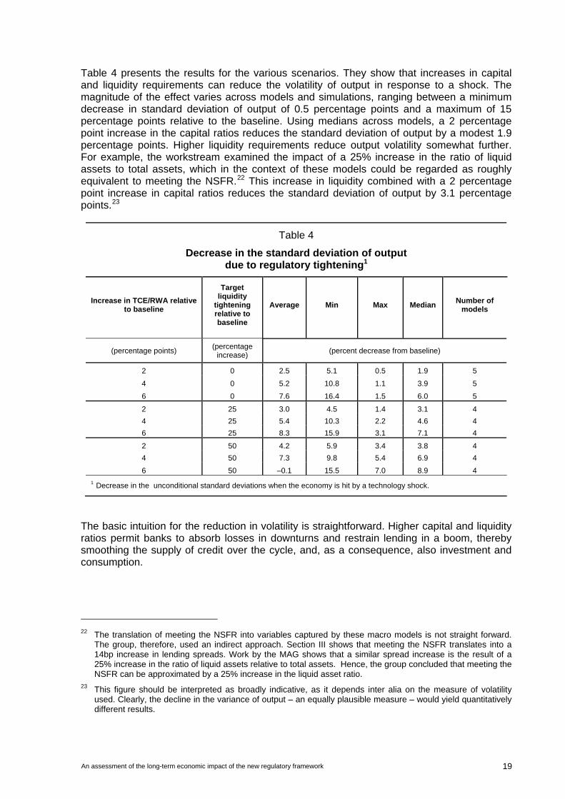
Table 4 presents the results for the various scenarios. They show that increases in capital and liquidity requirements can reduce the volatility of output in response to a shock. The magnitude of the effect varies across models and simulations, ranging between a minimum decrease in standard deviation of output of 0.5 percentage points and a maximum of 15 percentage points relative to the baseline. Using medians across models, a 2 percentage point increase in the capital ratios reduces the standard deviation of output by a modest 1.9 percentage points. Higher liquidity requirements reduce output volatility somewhat further. For example, the workstream examined the impact of a 25% increase in the ratio of liquid assets to total assets, which in the context of these models could be regarded as roughly equivalent to meeting the NSFR.22 This increase in liquidity combined with a 2 percentage point increase in capital ratios reduces the standard deviation of output by 3.1 percentage points.23
Table 4
Decrease in the standard deviation of output due to regulatory tightening1
Increase in TCE/RWA relative to baseline
Target liquidity
tightening relative to baseline
Average Min Max Median Number of
models
(percentage points) (percentage
increase) (percent decrease from baseline)
2 0 2.5 5.1 0.5 1.9 5
4 0 5.2 10.8 1.1 3.9 5
6 0 7.6 16.4 1.5 6.0 5
2 25 3.0 4.5 1.4 3.1 4
4 25 5.4 10.3 2.2 4.6 4
6 25 8.3 15.9 3.1 7.1 4
2 50 4.2 5.9 3.4 3.8 4
4 50 7.3 9.8 5.4 6.9 4
6 50 –0.1 15.5 7.0 8.9 4
1 Decrease in the unconditional standard deviations when the economy is hit by a technology shock.
The basic intuition for the reduction in volatility is straightforward. Higher capital and liquidity ratios permit banks to absorb losses in downturns and restrain lending in a boom, thereby smoothing the supply of credit over the cycle, and, as a consequence, also investment and consumption.
22 The translation of meeting the NSFR into variables captured by these macro models is not straight forward.
The group, therefore, used an indirect approach. Section III shows that meeting the NSFR translates into a 14bp increase in lending spreads. Work by the MAG shows that a similar spread increase is the result of a 25% increase in the ratio of liquid assets relative to total assets. Hence, the group concluded that meeting the NSFR can be approximated by a 25% increase in the liquid asset ratio.
23 This figure should be interpreted as broadly indicative, as it depends inter alia on the measure of volatility used. Clearly, the decline in the variance of output – an equally plausible measure – would yield quantitatively different results.
20 An assessment of the long-term economic impact of the new regulatory framework
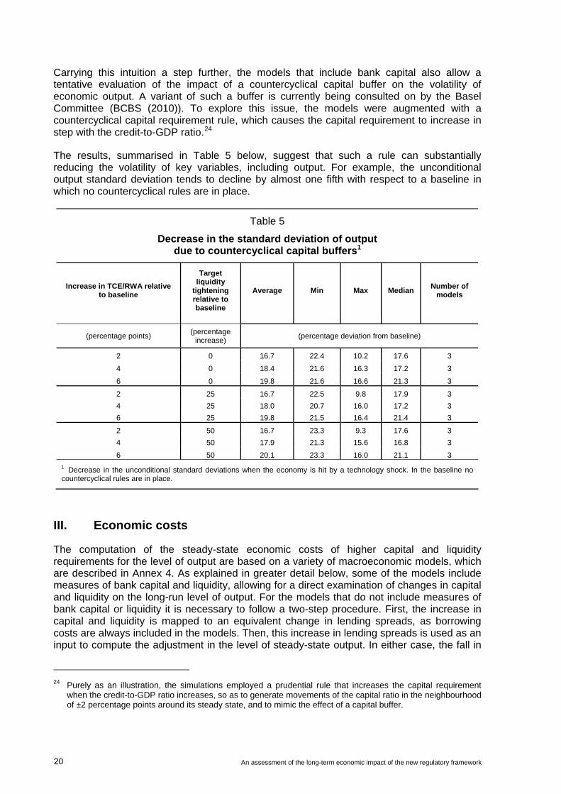
Carrying this intuition a step further, the models that include bank capital also allow a tentative evaluation of the impact of a countercyclical capital buffer on the volatility of economic output. A variant of such a buffer is currently being consulted on by the Basel Committee (BCBS (2010)). To explore this issue, the models were augmented with a countercyclical capital requirement rule, which causes the capital requirement to increase in step with the credit-to-GDP ratio.24
The results, summarised in Table 5 below, suggest that such a rule can substantially reducing the volatility of key variables, including output. For example, the unconditional output standard deviation tends to decline by almost one fifth with respect to a baseline in which no countercyclical rules are in place.
Table 5
Decrease in the standard deviation of output due to countercyclical capital buffers1
Increase in TCE/RWA relative to baseline
Target liquidity
tightening relative to baseline
Average Min Max Median Number of
models
(percentage points) (percentage
increase) (percentage deviation from baseline)
2 0 16.7 22.4 10.2 17.6 3
4 0 18.4 21.6 16.3 17.2 3
6 0 19.8 21.6 16.6 21.3 3
2 25 16.7 22.5 9.8 17.9 3
4 25 18.0 20.7 16.0 17.2 3
6 25 19.8 21.5 16.4 21.4 3
2 50 16.7 23.3 9.3 17.6 3
4 50 17.9 21.3 15.6 16.8 3
6 50 20.1 23.3 16.0 21.1 3
1 Decrease in the unconditional standard deviations when the economy is hit by a technology shock. In the baseline no countercyclical rules are in place.
III. Economic costs
The computation of the steady-state economic costs of higher capital and liquidity requirements for the level of output are based on a variety of macroeconomic models, which are described in Annex 4. As explained in greater detail below, some of the models include measures of bank capital and liquidity, allowing for a direct examination of changes in capital and liquidity on the long-run level of output. For the models that do not include measures of bank capital or liquidity it is necessary to follow a two-step procedure. First, the increase in capital and liquidity is mapped to an equivalent change in lending spreads, as borrowing costs are always included in the models. Then, this increase in lending spreads is used as an input to compute the adjustment in the level of steady-state output. In either case, the fall in
24 Purely as an illustration, the simulations employed a prudential rule that increases the capital requirement
when the credit-to-GDP ratio increases, so as to generate movements of the capital ratio in the neighbourhood of ±2 percentage points around its steady state, and to mimic the effect of a capital buffer.

An assessment of the long-term economic impact of the new regulatory framework 21
the level of output represents the economic cost of the regulatory change. This section describes the first, intermediate step and then considers the impact of the regulatory reform across the whole set of models used in the analysis.
The steady-state analysis assumes that the impact of higher capital and liquidity operates through the higher cost of credit. By focusing on price adjustments, the analysis does not capture any possible impact of credit rationing that might arise from more stringent requirements. The reason for this choice is precisely that the analysis focuses on the long-run steady state, after banks have fully adjusted to the new requirements. While banks might shrink their assets by rationing credit if the transition period is too short, the impact of credit rationing is likely to be much smaller in the long run, as markets have time to clear. Non-price effects are likely to be more important during the transition, and are thus considered in the work of the MAG.
III.A. Changes in lending spreads
This section describes the first step of the two-step process of calculating the impact of changing capital and liquidity requirements on economic output and welfare: the change in lending spreads. Capital and liquidity requirements are considered in turn.
While the analysis is based on a number of assumptions, it utilises information for a broad range of countries. The cornerstone of the analysis is a representative bank for each of 13 countries, drawing on income and balance sheet data averaged over a total of 6,660 banks for the 15-year period from 1993 to 2007.25 The resulting balance sheet and a set of costs of funds and returns on assets for each representative bank are assumed to represent a long-run average (steady state) that reflects each country’s institutional setting and regulatory framework. Table A3.1 in Annex 3 reports the weighted average bank balance sheet and income statement across the whole sample.26
III.A.1 The impact of higher capital requirements
Mapping the impact of the higher capital requirements on lending rates requires estimates of the cost of various sources of funding. The cost of equity is assumed to equal the 15-year average return on equity (ROE) for each country, which averages 14.8% across the countries in this sample.27 The cost of liabilities is based on short-term and long-term wholesale debt, and is calibrated to match the historical ratio of interest expense to total assets observed for each country. The computation assumes a fixed spread over deposits of 100 basis points for short-term debt and 200 basis points for long-term debt. These spreads are consistent with historical averages across the countries in this sample, and generate an upward sloping yield curve.28
The experiment assumes that the TCE/RWA ratio is raised by increasing equity and reducing long-term debt correspondingly. Importantly, it assumes (i) that any higher cost of funding
25 The countries considered in this analysis are: Australia, Canada, France, Germany, Italy, Japan, Korea,
Mexico, the Netherlands, Spain, Switzerland, the United Kingdom and the United States. 26 All variables are standardised by dividing by each bank’s total assets in each year. 27 Note that taking a 15-year average ROE may bias the overall cost estimates upwards if the last 15 years are
not reflective of the long-term cost of equity, perhaps because they were associated with a period of near-continuous economic expansion and extraordinary bank profitability in many countries.
28 Details on all the assumptions used in this analysis, and their impact on the results, are provided in Annex 3.

22 An assessment of the long-term economic impact of the new regulatory framework
associated with this change is fully recovered exclusively by raising loan rates – 100% pass-through; and (ii) that the costs of equity and of debt are not affected by the lower riskiness of the bank. As discussed in more detail below, this, together with the rather conservative assumption about the initial ROE, suggests that the results should be viewed as providing something close to an upper bound of the impact on loan spreads.
Next, the capital ratio for the representative bank in each country is increased by increments of 1 percentage point. All else equal, this reduces ROE.29 While part of the fall in ROE is offset by the smaller amount of debt outstanding, reducing the bank’s interest expense, the overall effect of the change in capital structure is to reduce net income as debt is substituted with more expensive equity. In line with the full-pass-through assumption, banks are assumed to pass on these additional costs to borrowers, raising the spreads charged on loans in order to exactly offset the increase in the cost of funding, keeping ROE unchanged at its historical average level.
Column A of Table 6 reports the results of this exercise. In order to keep ROE from changing, each percentage point increase in the ratio of TCE to RWA results in a median increase in lending spreads across countries of 13 basis points.
This result is obviously sensitive to a number of the assumptions in the analysis. For example, if the average ROE for the representative bank in steady state is 10.0% (rather than the 1993–2007 average of 14.8%), then the gap between the cost of equity and the cost of debt is smaller and the relative attractiveness of leverage is reduced.30 Based on this lower ROE assumption, a 1 percentage point increase in TCE/RWA can be offset by raising lending spreads by 7 basis points.
Moreover, banks could offset the loss of net income arising from meeting increased capital requirements through other means than raising loan rates. For example, banks could in principle (i) increase non-interest income (eg fees and commissions), (ii) reduce the rate paid on deposits, or (iii) reduce operating expenses. Any combination of these actions will generate higher net income and reduce the need to raise lending spreads.
It is possible to provide a sense of the magnitudes involved. The rise in lending spreads associated with a 1 percentage point increase in the capital ratio could be avoided by reducing operating expenses by 3.5% (median). Similarly, a 1.9 percentage point fall in median ROE is sufficient to absorb a 1 percentage point increase in the capital-to-RWA ratio.
Indeed, there are good reasons to believe that the cost of capital would decline in response to a reduction in bank leverage. As capital levels increase and the bank becomes safer, both of these costs should decline, further reducing the impact on lending spreads. And, in the limit, the change in the cost of capital could reduce to tax effects (Modigliani and Miller (1958)). Such a decline has not been considered in the estimates included in the table.
Academic studies have also provided estimates of the long-run costs of higher capital requirements. These confirm the conclusion that the median estimates in this report, used to derive the core measure of net benefits in section IV, are very conservative.
29 Return on equity (ROE) = net income / shareholders’ equity. 30 Academic studies which place the real cost of equity for banks in the region of 10% include Zimmer, S A and
R N McCauley (1991), King, M (2009), Capie, F and Billings, M (2004).
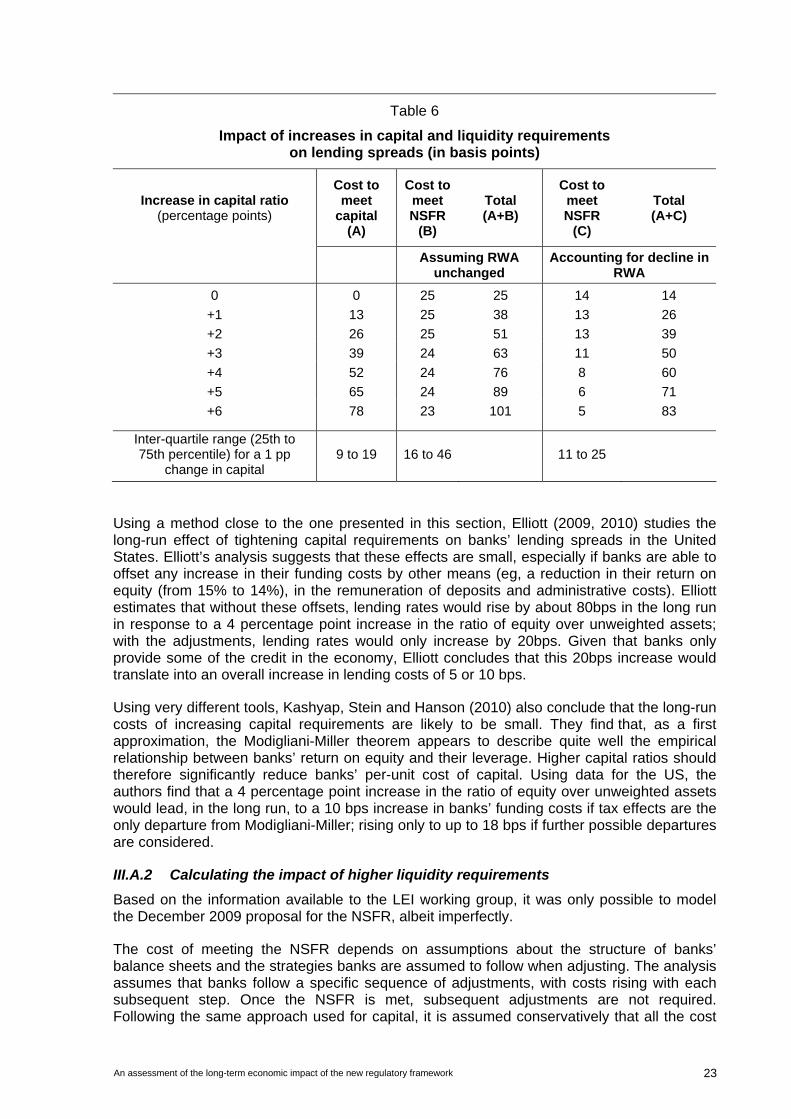
An assessment of the long-term economic impact of the new regulatory framework 23
Table 6
Impact of increases in capital and liquidity requirements on lending spreads (in basis points)
Increase in capital ratio (percentage points)
Cost to meet
capital (A)
Cost to meet NSFR
(B)
Total (A+B)
Cost to meet NSFR
(C)
Total (A+C)
Assuming RWA
unchanged Accounting for decline in
RWA
0 0 25 25 14 14
+1 13 25 38 13 26
+2 26 25 51 13 39
+3 39 24 63 11 50
+4 52 24 76 8 60
+5 65 24 89 6 71
+6 78 23 101 5 83
Inter-quartile range (25th to 75th percentile) for a 1 pp
change in capital 9 to 19 16 to 46 11 to 25
Using a method close to the one presented in this section, Elliott (2009, 2010) studies the long-run effect of tightening capital requirements on banks’ lending spreads in the United States. Elliott’s analysis suggests that these effects are small, especially if banks are able to offset any increase in their funding costs by other means (eg, a reduction in their return on equity (from 15% to 14%), in the remuneration of deposits and administrative costs). Elliott estimates that without these offsets, lending rates would rise by about 80bps in the long run in response to a 4 percentage point increase in the ratio of equity over unweighted assets; with the adjustments, lending rates would only increase by 20bps. Given that banks only provide some of the credit in the economy, Elliott concludes that this 20bps increase would translate into an overall increase in lending costs of 5 or 10 bps.
Using very different tools, Kashyap, Stein and Hanson (2010) also conclude that the long-run costs of increasing capital requirements are likely to be small. They find that, as a first approximation, the Modigliani-Miller theorem appears to describe quite well the empirical relationship between banks’ return on equity and their leverage. Higher capital ratios should therefore significantly reduce banks’ per-unit cost of capital. Using data for the US, the authors find that a 4 percentage point increase in the ratio of equity over unweighted assets would lead, in the long run, to a 10 bps increase in banks’ funding costs if tax effects are the only departure from Modigliani-Miller; rising only to up to 18 bps if further possible departures are considered.
III.A.2 Calculating the impact of higher liquidity requirements
Based on the information available to the LEI working group, it was only possible to model the December 2009 proposal for the NSFR, albeit imperfectly.
The cost of meeting the NSFR depends on assumptions about the structure of banks’ balance sheets and the strategies banks are assumed to follow when adjusting. The analysis assumes that banks follow a specific sequence of adjustments, with costs rising with each subsequent step. Once the NSFR is met, subsequent adjustments are not required. Following the same approach used for capital, it is assumed conservatively that all the cost
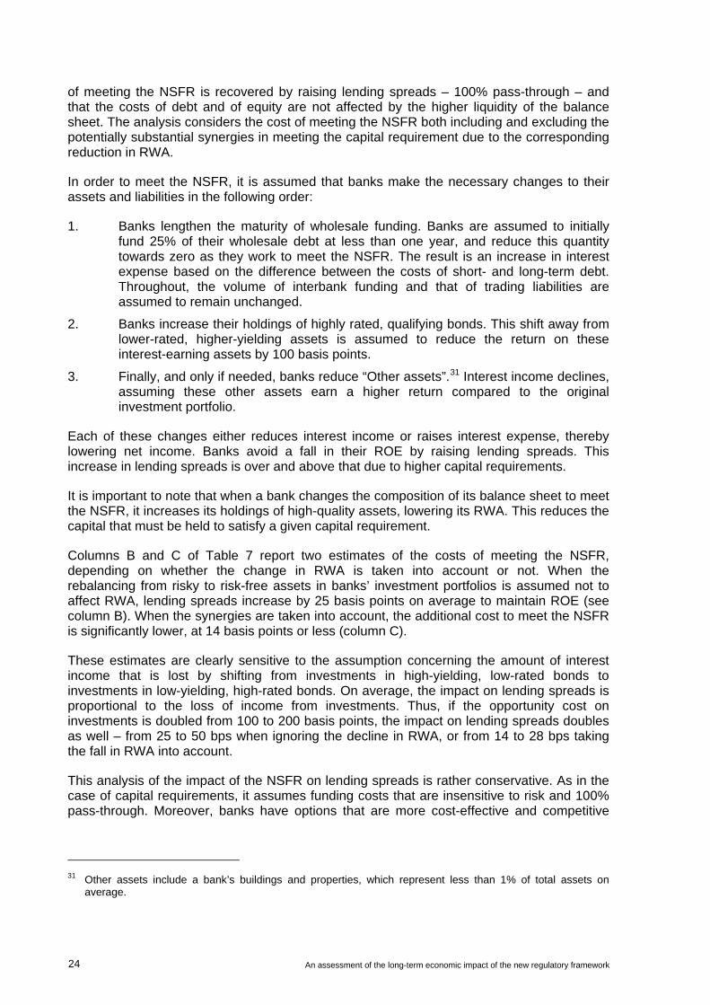
24 An assessment of the long-term economic impact of the new regulatory framework
of meeting the NSFR is recovered by raising lending spreads – 100% pass-through – and that the costs of debt and of equity are not affected by the higher liquidity of the balance sheet. The analysis considers the cost of meeting the NSFR both including and excluding the potentially substantial synergies in meeting the capital requirement due to the corresponding reduction in RWA.
In order to meet the NSFR, it is assumed that banks make the necessary changes to their assets and liabilities in the following order:
1. Banks lengthen the maturity of wholesale funding. Banks are assumed to initially fund 25% of their wholesale debt at less than one year, and reduce this quantity towards zero as they work to meet the NSFR. The result is an increase in interest expense based on the difference between the costs of short- and long-term debt. Throughout, the volume of interbank funding and that of trading liabilities are assumed to remain unchanged.
2. Banks increase their holdings of highly rated, qualifying bonds. This shift away from lower-rated, higher-yielding assets is assumed to reduce the return on these interest-earning assets by 100 basis points.
3. Finally, and only if needed, banks reduce “Other assets”.31 Interest income declines, assuming these other assets earn a higher return compared to the original investment portfolio.
Each of these changes either reduces interest income or raises interest expense, thereby lowering net income. Banks avoid a fall in their ROE by raising lending spreads. This increase in lending spreads is over and above that due to higher capital requirements.
It is important to note that when a bank changes the composition of its balance sheet to meet the NSFR, it increases its holdings of high-quality assets, lowering its RWA. This reduces the capital that must be held to satisfy a given capital requirement.
Columns B and C of Table 7 report two estimates of the costs of meeting the NSFR, depending on whether the change in RWA is taken into account or not. When the rebalancing from risky to risk-free assets in banks’ investment portfolios is assumed not to affect RWA, lending spreads increase by 25 basis points on average to maintain ROE (see column B). When the synergies are taken into account, the additional cost to meet the NSFR is significantly lower, at 14 basis points or less (column C).
These estimates are clearly sensitive to the assumption concerning the amount of interest income that is lost by shifting from investments in high-yielding, low-rated bonds to investments in low-yielding, high-rated bonds. On average, the impact on lending spreads is proportional to the loss of income from investments. Thus, if the opportunity cost on investments is doubled from 100 to 200 basis points, the impact on lending spreads doubles as well – from 25 to 50 bps when ignoring the decline in RWA, or from 14 to 28 bps taking the fall in RWA into account.
This analysis of the impact of the NSFR on lending spreads is rather conservative. As in the case of capital requirements, it assumes funding costs that are insensitive to risk and 100% pass-through. Moreover, banks have options that are more cost-effective and competitive
31 Other assets include a bank’s buildings and properties, which represent less than 1% of total assets on
average.
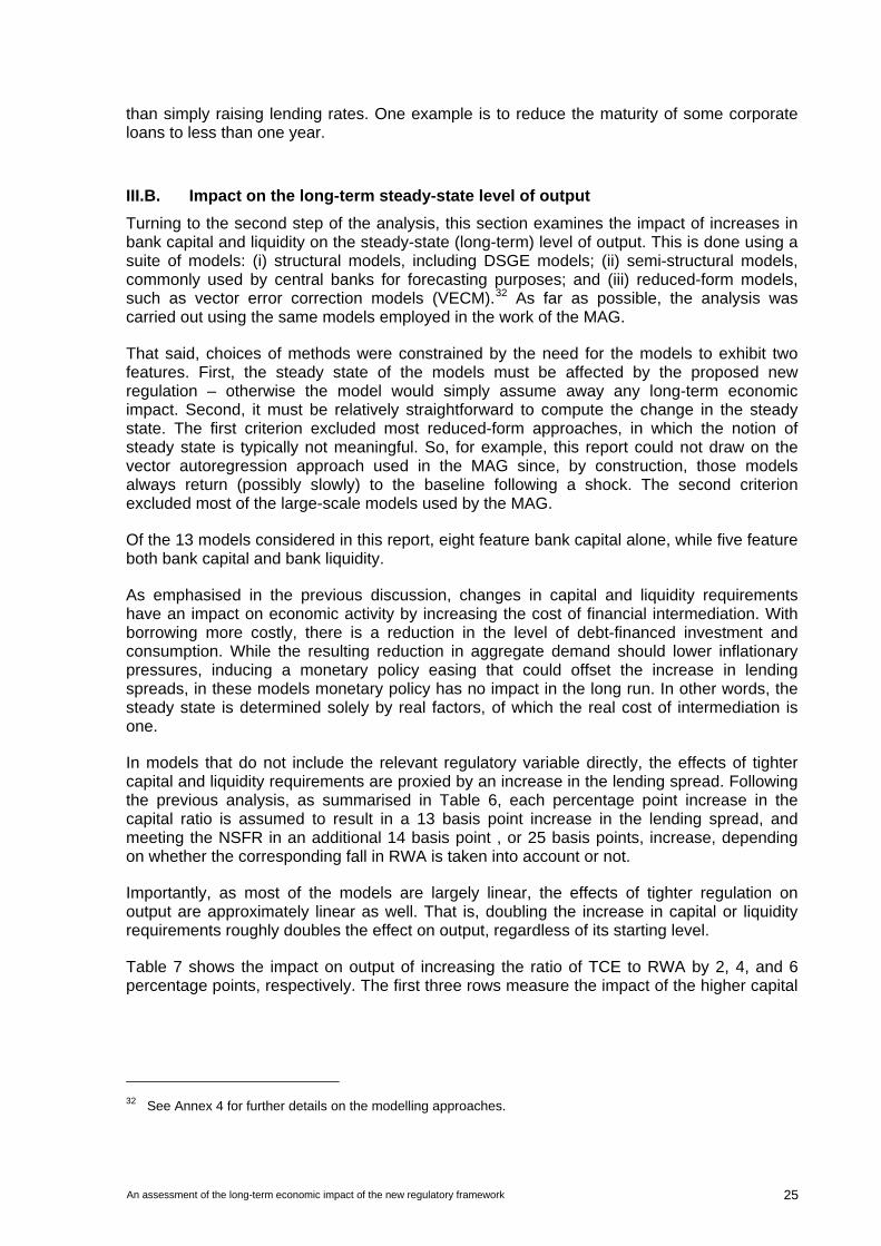
An assessment of the long-term economic impact of the new regulatory framework 25
than simply raising lending rates. One example is to reduce the maturity of some corporate loans to less than one year.
III.B. Impact on the long-term steady-state level of output
Turning to the second step of the analysis, this section examines the impact of increases in bank capital and liquidity on the steady-state (long-term) level of output. This is done using a suite of models: (i) structural models, including DSGE models; (ii) semi-structural models, commonly used by central banks for forecasting purposes; and (iii) reduced-form models, such as vector error correction models (VECM).32 As far as possible, the analysis was carried out using the same models employed in the work of the MAG.
That said, choices of methods were constrained by the need for the models to exhibit two features. First, the steady state of the models must be affected by the proposed new regulation – otherwise the model would simply assume away any long-term economic impact. Second, it must be relatively straightforward to compute the change in the steady state. The first criterion excluded most reduced-form approaches, in which the notion of steady state is typically not meaningful. So, for example, this report could not draw on the vector autoregression approach used in the MAG since, by construction, those models always return (possibly slowly) to the baseline following a shock. The second criterion excluded most of the large-scale models used by the MAG.
Of the 13 models considered in this report, eight feature bank capital alone, while five feature both bank capital and bank liquidity.
As emphasised in the previous discussion, changes in capital and liquidity requirements have an impact on economic activity by increasing the cost of financial intermediation. With borrowing more costly, there is a reduction in the level of debt-financed investment and consumption. While the resulting reduction in aggregate demand should lower inflationary pressures, inducing a monetary policy easing that could offset the increase in lending spreads, in these models monetary policy has no impact in the long run. In other words, the steady state is determined solely by real factors, of which the real cost of intermediation is one.
In models that do not include the relevant regulatory variable directly, the effects of tighter capital and liquidity requirements are proxied by an increase in the lending spread. Following the previous analysis, as summarised in Table 6, each percentage point increase in the capital ratio is assumed to result in a 13 basis point increase in the lending spread, and meeting the NSFR in an additional 14 basis point , or 25 basis points, increase, depending on whether the corresponding fall in RWA is taken into account or not.
Importantly, as most of the models are largely linear, the effects of tighter regulation on output are approximately linear as well. That is, doubling the increase in capital or liquidity requirements roughly doubles the effect on output, regardless of its starting level.
Table 7 shows the impact on output of increasing the ratio of TCE to RWA by 2, 4, and 6 percentage points, respectively. The first three rows measure the impact of the higher capital
32 See Annex 4 for further details on the modelling approaches.
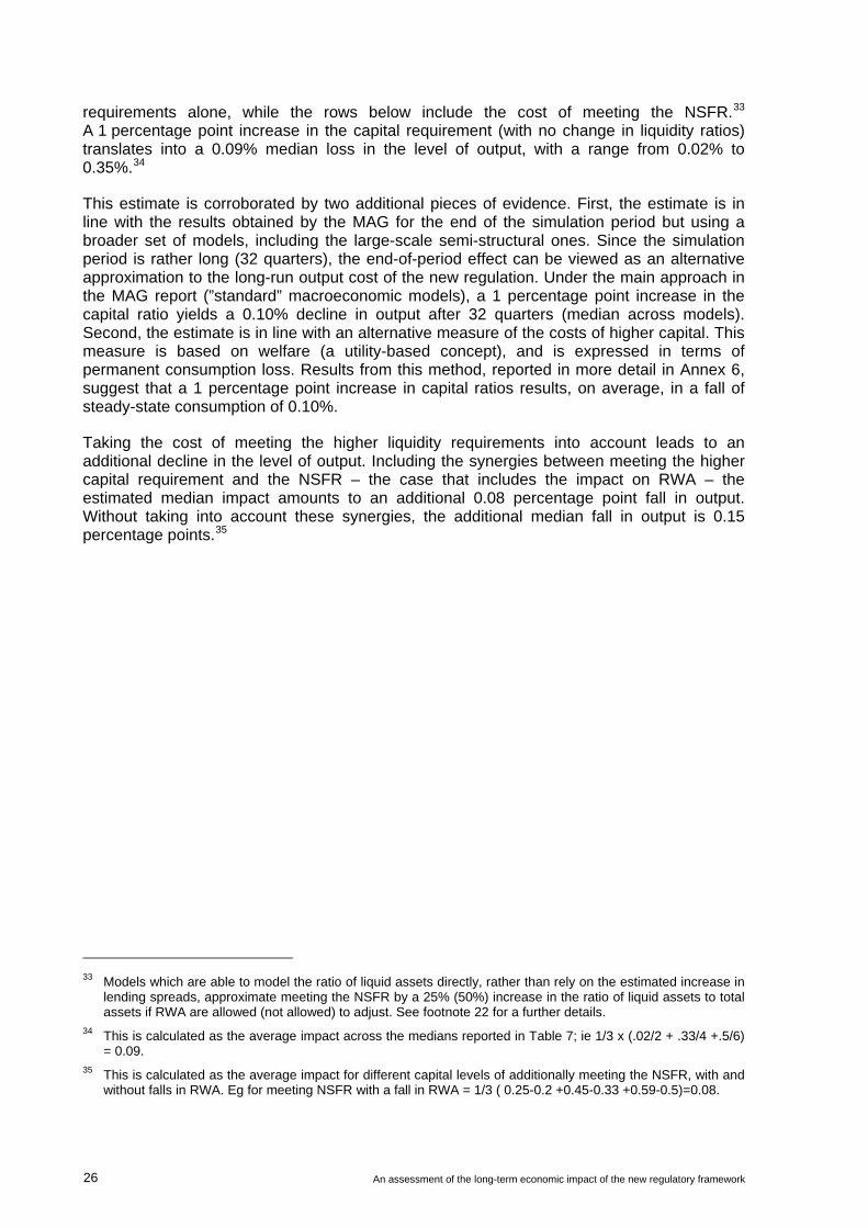
26 An assessment of the long-term economic impact of the new regulatory framework
requirements alone, while the rows below include the cost of meeting the NSFR.33 A 1 percentage point increase in the capital requirement (with no change in liquidity ratios) translates into a 0.09% median loss in the level of output, with a range from 0.02% to 0.35%.34
This estimate is corroborated by two additional pieces of evidence. First, the estimate is in line with the results obtained by the MAG for the end of the simulation period but using a broader set of models, including the large-scale semi-structural ones. Since the simulation period is rather long (32 quarters), the end-of-period effect can be viewed as an alternative approximation to the long-run output cost of the new regulation. Under the main approach in the MAG report (”standard” macroeconomic models), a 1 percentage point increase in the capital ratio yields a 0.10% decline in output after 32 quarters (median across models). Second, the estimate is in line with an alternative measure of the costs of higher capital. This measure is based on welfare (a utility-based concept), and is expressed in terms of permanent consumption loss. Results from this method, reported in more detail in Annex 6, suggest that a 1 percentage point increase in capital ratios results, on average, in a fall of steady-state consumption of 0.10%.
Taking the cost of meeting the higher liquidity requirements into account leads to an additional decline in the level of output. Including the synergies between meeting the higher capital requirement and the NSFR – the case that includes the impact on RWA – the estimated median impact amounts to an additional 0.08 percentage point fall in output. Without taking into account these synergies, the additional median fall in output is 0.15 percentage points.35
33 Models which are able to model the ratio of liquid assets directly, rather than rely on the estimated increase in
lending spreads, approximate meeting the NSFR by a 25% (50%) increase in the ratio of liquid assets to total assets if RWA are allowed (not allowed) to adjust. See footnote 22 for a further details.
34 This is calculated as the average impact across the medians reported in Table 7; ie 1/3 x (.02/2 + .33/4 +.5/6) = 0.09.
35 This is calculated as the average impact for different capital levels of additionally meeting the NSFR, with and without falls in RWA. Eg for meeting NSFR with a fall in RWA = 1/3 ( 0.25-0.2 +0.45-0.33 +0.59-0.5)=0.08.
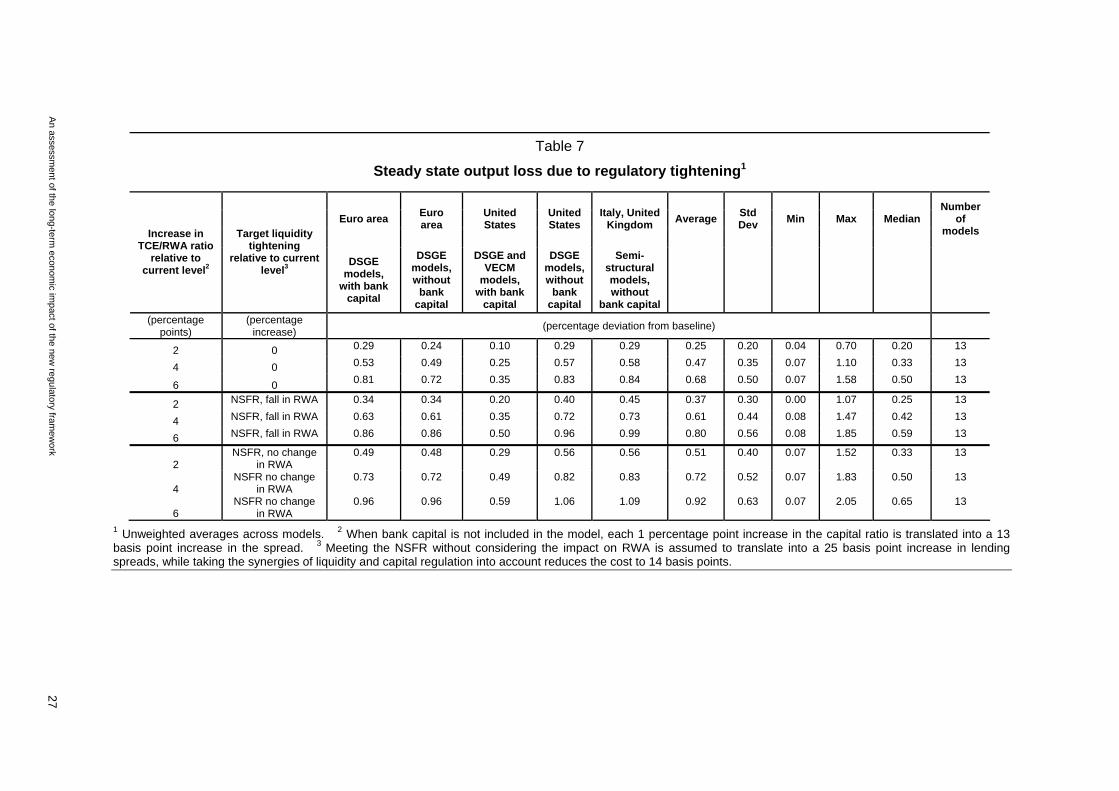
An assessm
ent of the long-term econom
ic impact of the new
regulatory framew
ork 27
Table 7
Steady state output loss due to regulatory tightening1
Euro area Euro area
United States
United States
Italy, United Kingdom
Average Std Dev
Min Max Median Number
of models Increase in
TCE/RWA ratio relative to
current level2
Target liquidity tightening
relative to current level3
DSGE models,
with bank capital
DSGE models, without
bank capital
DSGE and VECM
models, with bank
capital
DSGE models, without
bank capital
Semi-structural models, without
bank capital
(percentage points)
(percentage increase)
(percentage deviation from baseline)
2 0 0.29 0.24 0.10 0.29 0.29 0.25 0.20 0.04 0.70 0.20 13
4 0 0.53 0.49 0.25 0.57 0.58 0.47 0.35 0.07 1.10 0.33 13
6 0 0.81 0.72 0.35 0.83 0.84 0.68 0.50 0.07 1.58 0.50 13
2 NSFR, fall in RWA 0.34 0.34 0.20 0.40 0.45 0.37 0.30 0.00 1.07 0.25 13
4 NSFR, fall in RWA 0.63 0.61 0.35 0.72 0.73 0.61 0.44 0.08 1.47 0.42 13
6 NSFR, fall in RWA 0.86 0.86 0.50 0.96 0.99 0.80 0.56 0.08 1.85 0.59 13
2 NSFR, no change
in RWA 0.49 0.48 0.29 0.56 0.56 0.51 0.40 0.07 1.52 0.33 13
4 NSFR no change
in RWA 0.73 0.72 0.49 0.82 0.83 0.72 0.52 0.07 1.83 0.50 13
6 NSFR no change
in RWA 0.96 0.96 0.59 1.06 1.09 0.92 0.63 0.07 2.05 0.65 13
1 Unweighted averages across models. 2 When bank capital is not included in the model, each 1 percentage point increase in the capital ratio is translated into a 13 basis point increase in the spread. 3 Meeting the NSFR without considering the impact on RWA is assumed to translate into a 25 basis point increase in lending spreads, while taking the synergies of liquidity and capital regulation into account reduces the cost to 14 basis points.
28 An assessment of the long-term economic impact of the new regulatory framework
IV. Net benefits
This section brings together the analysis of the economic benefits and costs carried out so far. It first derives a summary estimate of the net benefits associated with the reduction in the incidence of banking crises. Following the previous analysis, these calculations are in terms of the level of output. For that reason, the benefits that arise from a lower volatility of output are not included at this stage. The section then highlights a broader set of considerations, not explicitly included in the summary estimate, that need to be taken into account when forming an overall assessment. The main conclusion is that, on balance, there is considerable room to raise capital and liquidity requirements while still yielding net benefits.
In making an assessment of the net benefits in terms of the level of output per year, it is important to understand the relationship between benefits and costs over time. Higher capital and liquidity reduce the annual probability (and arguably the severity) of banking crises, but the costs of the crisis are not limited to the crisis year, as they have long-lasting, possibly permanent, effects on output. The cost of tighter regulation is the yearly cost in terms of output forgone. The more permanent the effects of a crisis are on output growth, the larger is the annual net benefit.
An apt analogy is with a museum’s security system. The system lowers the probability of a break-in, but if the break-in takes place, the costs can be substantial and may even be permanent, if unique works of art are irreparably damaged or lost forever. The yearly benefit reflects this lower probability times these long-lasting effects. The yearly cost includes the running costs, in the form of wages for staff, maintenance and the like. The benefits and costs of regulation in any given year are similar: the benefit is the annual reduction in the probability of a crisis in the given year times its (discounted) long-lasting costs, which extend beyond that year; the cost is the lower annual output during that year.
Table 8 and Graph 4 provide summaries of the results from the previous sections of the report. They show the estimated benefits and costs and corresponding net benefits measured by the percentage change in the yearly level of output. These changes should be interpreted relative to the pre-reform steady state, proxied by the historical average level of the capital ratio (7%) and frequency of banking crises without the liquidity requirements being met (the first row in Table 8 and the origin in the graph). The table and the graph show a range of results, reflecting various estimates of the costs of banking crises, depending on whether costs are estimated as permanent but moderate – which also corresponds to the median estimate across all comparable studies (red line) – or only as temporary (green line). Table 8 also presents the estimates of net benefits when the costs of banking crises are estimated as large and permanent. As noted previously, taking a conservative approach, the report places less emphasis on the latter results. In all cases the results assume that institutions pass the added costs arising from strengthened regulations on to borrowers in their entirety while maintaining pre-reform levels for the ROE, interest costs of liabilities and operating expenses. Thus, in this sense, the costs of meeting the standards may be close to an upper bound.36
36 The assessment of the liquidity regulations focuses on the NSFR, as defined in the December 2009 proposal.
At the same time, it also provides information pertinent to the assessment of the LCR.
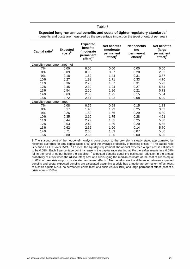
An assessment of the long-term economic impact of the new regulatory framework 29
Table 8
Expected long-run annual benefits and costs of tighter regulatory standards1 (benefits and costs are measured by the percentage impact on the level of output per year)
Capital ratio2 Expected costs3
Expected benefits
(moderate permanent
effect)4
Net benefits (moderate permanent
effect)5
Net benefits (no
permanent effect)5
Net benefits (large
permanent effect)5
Liquidity requirement not met 7% 0.00 0.00 0.00 0.00 0.00 8% 0.09 0.96 0.87 0.20 2.32 9% 0.18 1.62 1.44 0.31 3.87
10% 0.27 1.98 1.71 0.33 4.70 11% 0.36 2.23 1.87 0.31 5.23 12% 0.45 2.39 1.94 0.27 5.54 13% 0.54 2.50 1.96 0.21 5.73 14% 0.63 2.58 1.95 0.15 5.84 15% 0.72 2.64 1.92 0.08 5.90
Liquidity requirement met 7% 0.08 0.76 0.68 0.15 1.83 8% 0.17 1.40 1.23 0.25 3.33 9% 0.26 1.82 1.56 0.29 4.30
10% 0.35 2.10 1.75 0.28 4.91 11% 0.44 2.29 1.85 0.25 5.30 12% 0.53 2.42 1.89 0.20 5.55 13% 0.62 2.52 1.90 0.14 5.70 14% 0.71 2.60 1.89 0.07 5.80 15% 0.80 2.65 1.85 0.00 5.85
1 The starting point of the net-benefit analysis corresponds to the pre-reform steady state, approximated by historical averages for total capital ratios (7%) and the average probability of banking crises. 2 The capital ratio is defined as TCE over RWA. 3 To meet the liquidity requirement, the annual expected output cost is estimated to be 0.08%. Each 1 percentage point increase in the capital ratio starting at 7% thereafter results in a 0.09% fall in the level of output below the baseline. 4 Expected benefits equal the estimated reduction in the annual probability of crisis times the (discounted) cost of a crisis using the median estimate of the cost of crises equal to 63% of pre-crisis output ( moderate permanent effect). 5 Net benefits are the difference between expected benefits and costs; expected benefits are calculated assuming a crisis has a moderate permanent effect (cost of a crisis equals 63%), no permanent effect (cost of a crisis equals 19%) and large permanent effect (cost of a crisis equals 158%).
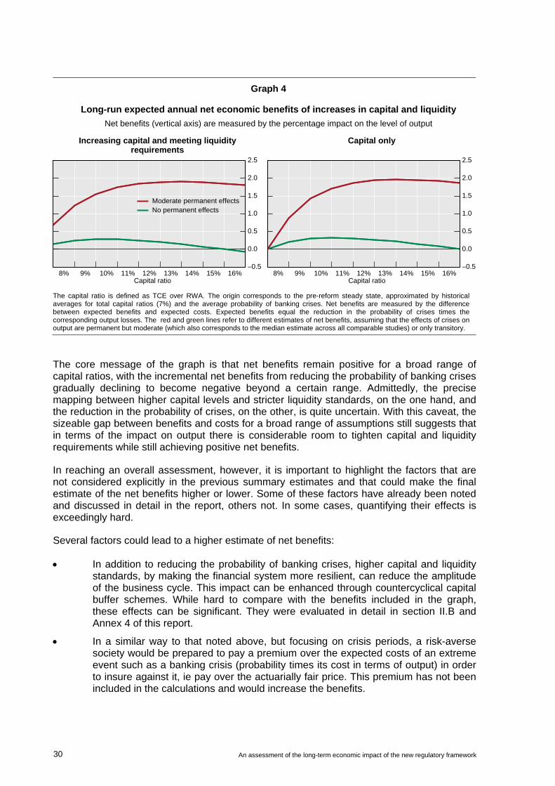
30 An assessment of the long-term economic impact of the new regulatory framework
Graph 4
Long-run expected annual net economic benefits of increases in capital and liquidity
Net benefits (vertical axis) are measured by the percentage impact on the level of output
Increasing capital and meeting liquidity requirements
Capital only
–0.5
0.0
0.5
1.0
1.5
2.0
2.5
8% 9% 10% 11% 12% 13% 14% 15% 16%Capital ratio
Moderate permanent effectsNo permanent effects
–0.5
0.0
0.5
1.0
1.5
2.0
2.5
8% 9% 10% 11% 12% 13% 14% 15% 16%Capital ratio
The capital ratio is defined as TCE over RWA. The origin corresponds to the pre-reform steady state, approximated by historical averages for total capital ratios (7%) and the average probability of banking crises. Net benefits are measured by the difference between expected benefits and expected costs. Expected benefits equal the reduction in the probability of crises times the corresponding output losses. The red and green lines refer to different estimates of net benefits, assuming that the effects of crises on output are permanent but moderate (which also corresponds to the median estimate across all comparable studies) or only transitory.
The core message of the graph is that net benefits remain positive for a broad range of capital ratios, with the incremental net benefits from reducing the probability of banking crises gradually declining to become negative beyond a certain range. Admittedly, the precise mapping between higher capital levels and stricter liquidity standards, on the one hand, and the reduction in the probability of crises, on the other, is quite uncertain. With this caveat, the sizeable gap between benefits and costs for a broad range of assumptions still suggests that in terms of the impact on output there is considerable room to tighten capital and liquidity requirements while still achieving positive net benefits.
In reaching an overall assessment, however, it is important to highlight the factors that are not considered explicitly in the previous summary estimates and that could make the final estimate of the net benefits higher or lower. Some of these factors have already been noted and discussed in detail in the report, others not. In some cases, quantifying their effects is exceedingly hard.
Several factors could lead to a higher estimate of net benefits:
In addition to reducing the probability of banking crises, higher capital and liquidity standards, by making the financial system more resilient, can reduce the amplitude of the business cycle. This impact can be enhanced through countercyclical capital buffer schemes. While hard to compare with the benefits included in the graph, these effects can be significant. They were evaluated in detail in section II.B and Annex 4 of this report.
In a similar way to that noted above, but focusing on crisis periods, a risk-averse society would be prepared to pay a premium over the expected costs of an extreme event such as a banking crisis (probability times its cost in terms of output) in order to insure against it, ie pay over the actuarially fair price. This premium has not been included in the calculations and would increase the benefits.
An assessment of the long-term economic impact of the new regulatory framework 31
The expected costs of crises are based on data from historical episodes featuring large-scale government intervention to minimise the negative effects on output. In the absence of such intervention, the average costs of banking crises are likely to be significantly higher. In addition, the discount rate used to estimate the present value of the multi-year cost of crises is quite conservative.
To the extent that higher capital and liquidity requirements also reduce the severity of crises, the benefits will be higher.
The analysis assumes full pass-through of the higher funding costs/lower yield from investments to loan rates. However, in the long run it is reasonable to expect that, by reducing banks’ riskiness, higher capital and liquidity requirements should lead to lower debt and equity costs. Moreover, once adjustment is complete, differences between the cost of equity and debt could reduce to tax effects. Banks could also adjust by increasing efficiency or reducing operating expenses. These effects would substantially reduce the estimated long-run costs.
To the extent that greater intermediation is provided by the non-bank sector, the estimated costs will be lower.
Similarly, there are a number of factors that could reduce the net benefits:
The existing literature, which is the basis for this report’s estimates of the costs of banking crises, may overestimate the costs of banking crises. Possible reasons include: overestimation of the underlying growth path prior to the crises; failure to account for the temporarily higher growth during that phase; and failure to fully control for factors other than a banking crises per se that may contribute to output declines during the crisis and beyond, including a failure to accurately reflect causal relationships.
Capital and liquidity requirements may be less effective in reducing the probability of banking crises than suggested by the approaches used in the study. This would reduce the overall net benefits for a given level of the requirements. However, to the extent that net benefits remain positive, it would also imply that the requirements would need to be raised by more in order to achieve a given net benefit.
Shifting of risk into the non-regulated sector could reduce the financial stability benefits.
The results of the impact of regulatory requirements on lending spreads are based on aggregate balance sheets within individual countries, so that they do not consider the incidence of the requirements across institutions. They implicitly assume that the institutions that fall short of the requirements (ie, that are constrained) do not react more than those with excess capital or liquidity (ie, that are unconstrained). These effects may not be purely distributional.
As a final caveat, the results summarised above reflect the estimated net benefits associated with higher capital and liquidity standards, averaged across a number of countries over an extended period. Clearly, there is a range of uncertainty around estimates of central tendencies, reflecting data limitations and the need for various modelling assumptions. In addition, the estimated net benefits may be higher or lower in individual cases.
32 An assessment of the long-term economic impact of the new regulatory framework
Annex 1
Costs of crises: a literature survey
There is a growing research literature analysing the costs of banking crises. This annex surveys that literature, explaining the methodologies used and providing a summary of the quantitative results.
Methodologies
The research literature uses a variety of approaches to measure the cost of banking crises. In what follows these are classified in groups depending on two key dimensions: the period over which they measure the impact of crises and the type of metric used to calculate their cost. This section discusses these two dimensions by reference to Graph 1 in the main text, which illustrates a stylised path of a crisis episode. Table 1 applies the same classification to the findings in the literature.
The first dimension relates the two points in time (or phases of a crisis episode) chosen as reference points for the measurement of costs. There are four types of approach. The first type focuses on the period between the GDP peak prior to the crisis and the subsequent through after the onset of the crisis (time between A and B in Graph 1). The second type defines the crisis period from the cyclical peak to the time that the GDP growth rate recovers to its pre-crisis level (between A and C in Graph 1). It is important to note that this point is not equivalent to that when GDP returns to its pre-crisis trend path. In fact, at that point GDP would be necessarily below that trend because (by definition) the economy has not undergone a catch-up period of faster than average growth in order to recover the ground lost during the crisis. The third type of approach defines the crisis period as lasting until the level of GDP returns to its pre-crisis trend path (between A and D). Studies that use expert judgement or set a prespecified fixed length for all crises would fall under this category, since they tend to come to similar conclusions. Finally, the fourth type of approach allows for the possibility of permanent effects of crises on the level of GDP (ie a downward shift in the growth path), hence effectively looking at an infinite horizon.
The second dimension in the classification of approaches relates to the metric used for the costs of crises. One approach focuses on the gap between potential or trend output and output at the end of a specific phase of the crisis. This gives a measure of how much output falls between two points in time, but it does not reflect the duration of the episode and, hence, the cumulative losses over the same period. For crises with permanent effects the corresponding metric would be the gap between the pre-crisis and post-crisis GDP trends (δ in Graph 1). The second approach looks instead at the cumulative losses from the onset of the crisis until the (variously defined) end of the crisis. For crises that have long-lasting (multi-year or permanent) effects the calculation of the cumulative costs would entail some form of discounting (see discussion below).
Table A1.1 lists different studies grouped along these two dimensions together with their estimates of the costs of the average crisis. The first three groups of studies adopt as metric the difference in levels between two different points in time. The first of these uses the simplest approach, which is to measure costs by considering the peak-to-trough drop in output (ie relative difference in GDP between point A and point B in Graph 1). The second group assumes that crises end once output growth returns to its pre-crisis trend (ie relative difference in GDP between point A and point D). Typically studies that follow this approach
An assessment of the long-term economic impact of the new regulatory framework 33
estimate the total impact on the level of GDP by calculating the sum of deviations of the post-crisis growth rate from the pre-crisis trend growth. For short crises, this is approximately the difference between trend and actual levels of output at point C.37 Generally, trend growth in these studies is calculated as the historical average growth over a period that ranges (depending on the study) between three and 10 years prior to the crisis.38 An alternative approach to measuring the differential between actual and potential growth is to use regression analysis to estimate the impact on GDP growth following a banking crisis. Two papers (Hutchinson and Neuberger (2005) and Demirgüç-Kunt et al (2006)) rely on this method. They find that crises affect growth negatively for two to three years. The third group of studies that measure the drop in the level of GDP focus on permanent effects (δ in Graph 1) and follow Cerra and Saxena (2008). They estimate the impact on GDP (more specifically, GDP growth) by using panel regressions for a group of countries that experienced banking crises. The regressors include lags of the dependent variable and/or other explanatory variables, as well as a dummy that flags the beginning of a banking crisis. The dummy variable allows the simulation of impulse response functions as shown in Graph A1.1.
The last two groups of studies summarised in Table A1.1 look at the cumulative effect on GDP, a better measure of the overall economic costs of banking crises. Less than half the studies in the literature calculate cumulative costs explicitly by summing across the difference between the actual level of GDP and its trend over the crisis period (as defined in each study).39 The trend of output is determined in different ways: as the historical average growth;40 as weighted average of past and world growth; by using the Hodrick-Prescott filter; or by reference to estimates of potential output (eg from OECD). The first of these two groups of studies does not allow for permanent output effects becausethe length of a crisis (ie the period over which its effects are estimated) is assumed to be finite.41 The second and last group of studies does allow for the possiblity of permanent effects. Boyd et al (2005) use two methods of calculating long-run costs after a crisis. The first method is more conservative and uses only actual GDP for the countries that had a crisis several years prior to the end of the sample (the results are listed under Method 1 in Table A1.1). In order to assess the full cumulative costs into the infinite horizon the authors use projections of both GDP and potential output for all crisis countries (these results are labelled Method 2 in Table A1.1). Haldane (2010) quantifies the costs of the current financial crisis by looking at the present value of output losses for the United Kingdom and the world. To provide a range of
37 All studies following this approach express the measured costs in total growth forgone during the assumed
period of the crisis. Assuming that discount rates equal trend growth rates, the measured costs are also approximately the costs relative to pre-crisis GDP, especially if crises are not too long. Hoggarth et al (2002) prove mathematically that the difference is actually underestimated for crises lasting longer than two years, as the approach does not recognise the reduction in output levels in the previous years.
38 Interestingly, this choice of trend implies that in some cases actual growth never reaches the pre-crisis trend growth. This is a sign of permanent effects, although the studies disregard this possibility. The crises in Mexico (1981) and or Japan (1992) are cases in point.
39 Except for Boyd et al (2005), costs are expressed relative to trend GDP. Assuming that discount rates equal trend growth rates, the measured costs are also the costs relative to pre-crisis GDP.
40 In comparison to other methods, relying on historical averages may overestimate trend output. This is particularly true is averages are calculated over shorter periods, as many banking crises tend to be preceded by unsustainable booms. A higher estimate of trend would imply higher costs of crises.
41 Some studies fix the length of crises at four years (eg Laeven and Valencia (2008)) or determine it on the basis of expert judgment (eg Hoggarth et al (2002)) or allow it to be determined endogenously by assuming that crises end when the level of GDP returns to its pre-crisis level (eg Cecchetti et al (2009)) or to the pre-crisis trend (eg Haugh et al (2009)).
34 An assessment of the long-term economic impact of the new regulatory framework
estimates, the analysis assumes that different fractions of output losses experienced in 2009 are permanent (25%, 50% and 100%). Losses are expressed relative to 2009 output.
A key parameter that influences the magnitude of cumulative losses is the choice of discount factor, especially in the case of studies that find permanent effects. Table A1.1 reports the average output losses shown in each study, even though different studies are based on different assumptions. For example, Boyd et al (2005) use a discount rate of 5%, while Haldane (2010) uses 2.5%. In this report, to provide a conservative estimate, permanent drops in steady-state output (ie those in the third group of studies reported in Table A1.1) are converted into cumulative losses (CL) by discounting future losses with a 5% discount rate (ie CL = δ/(1-α) with the discount factor α = 1/(1+5%)). A a lower (higher) discount rate would imply higher (lower) costs.
One paper in the literature (Ramirez (2009) finds that banking crises have long-lasting effects on long-term growth rates, no just the level of output (see Table A1.3). The study relies on data from 1894 in the United States. Using a panel of all US states and controlling for other factors, the analysis finds that increasing banking fragility (measured as the ratio of deposits in failed banks over total deposits) by 1% reduces the average annual growth rate between 1900 and 1930 by 2–5%.
Results
Table A1.1 shows that results in the literature are surprisingly consistent.
Studies in the first two groups, which compare GDP at the beginning of the crisis to the trough or to the point when its growth recovers, find a drop of around 10% relative to pre-crisis GDP. Costs tend to be somewhat lower for samples ending in the late 1990s (IMF (1998), Bordo et al (2001) Hoggarth et al (2002)). The results of these two groups are not taken into account when analysing the range and median of cumulative output losses of banking crises. The reason is that they refer to the difference in GDP between two points in time and, without some indication about the length of crises, they cannot be made comparable to the cumulative measure of costs adopted in this report.
Within the third group of studies, which measure point-in-time losses in the presence of permanent effects (δ in the main text), there is a considerable difference between those that measure deviations of potential output (eg Barrell et al (2010a) or Furceri and Mourougane (2009)) or deviations of actual output (eg Cerra and Saxena (2008), Turini et al (2010), IMF (2009), Furceri and Zdzienicka (2010)). The former studies find a permanent drop of 2% after a banking crisis, while the latter find effects of the order of 7.5–10%. The figures reported in the first column of Table A1.1 for this group of studies convert the estimates of a permanent drop in the level of GDP to a cumulative loss figure that is comparable to that reported by the next group of studies. The calculatoin was based on a 5% discount rate, as described above, and it corresponds to cumulative losses in the range of 42–210% relative to pre-crisis GDP.
The cumulative loss estimates listed in Table A1.1 for the fourth and fifth group of studies are reported directly by these papers. They correspond to the average effect found across all crises in each study (Table A1.2 reports episode-specific loss figures for BCBS countries as reported in the subset of all studies that provide the disaggregate estimates).
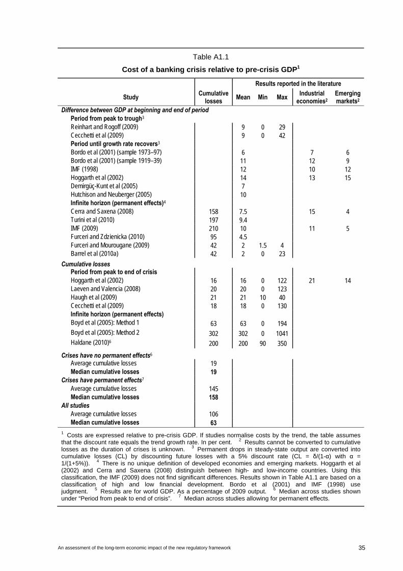
An assessment of the long-term economic impact of the new regulatory framework 35
Table A1.1
Cost of a banking crisis relative to pre-crisis GDP1
Results reported in the literature
Study Cumulative losses Mean Min Max Industrial
economies2 Emerging markets2
Difference between GDP at beginning and end of period Period from peak to trough3 Reinhart and Rogoff (2009) 9 0 29 Cecchetti et al (2009) 9 0 42 Period until growth rate recovers3 Bordo et al (2001) (sample 1973–97) 6 7 6 Bordo et al (2001) (sample 1919–39) 11 12 9 IMF (1998) 12 10 12 Hoggarth et al (2002) 14 13 15 Demirgüç-Kunt et al (2005) 7 Hutchison and Neuberger (2005) 10 Infinite horizon (permanent effects)4 Cerra and Saxena (2008) 158 7.5 15 4 Turini et al (2010) 197 9.4 IMF (2009) 210 10 11 5 Furceri and Zdzienicka (2010) 95 4.5 Furceri and Mourougane (2009) 42 2 1.5 4 Barrel et al (2010a) 42 2 0 23
Cumulative losses Period from peak to end of crisis Hoggarth et al (2002) 16 16 0 122 21 14 Laeven and Valencia (2008) 20 20 0 123 Haugh et al (2009) 21 21 10 40 Cecchetti et al (2009) 18 18 0 130 Infinite horizon (permanent effects)
Boyd et al (2005): Method 1 63 63 0 194
Boyd et al (2005): Method 2 302 302 0 1041
Haldane (2010)6 200 200 90 350
Crises have no permanent effects6
Average cumulative losses 19 Median cumulative losses 19 Crises have permanent effects7 Average cumulative losses 145 Median cumulative losses 158 All studies Average cumulative losses 106 Median cumulative losses 63 1 Costs are expressed relative to pre-crisis GDP. If studies normalise costs by the trend, the table assumes that the discount rate equals the trend growth rate. In per cent. 2 Results cannot be converted to cumulative losses as the duration of crises is unknown. 3 Permanent drops in steady-state output are converted into cumulative losses (CL) by discounting future losses with a 5% discount rate (CL = δ/(1-α) with α = 1/(1+5%)). 4 There is no unique definition of developed economies and emerging markets. Hoggarth et al (2002) and Cerra and Saxena (2008) distinguish between high- and low-income countries. Using this classification, the IMF (2009) does not find significant differences. Results shown in Table A1.1 are based on a classification of high and low financial development. Bordo et al (2001) and IMF (1998) use judgment. 5 Results are for world GDP. As a percentage of 2009 output. 6 Median across studies shown under “Period from peak to end of crisis”. 7 Median across studies allowing for permanent effects.
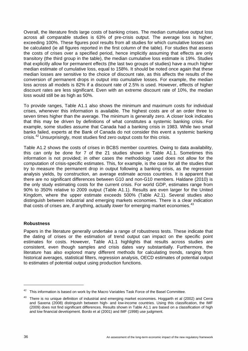
36 An assessment of the long-term economic impact of the new regulatory framework
Overall, the literature finds large costs of banking crises. The median cumulative output loss across all comparable studies is 63% of pre-crisis output. The average loss is higher, exceeding 100%. These figures pool results from all studies for which cumulative losses can be calculated (ie all figures reported in the first column of the table). For studies that assess the costs of crises over a specified period, hence implicitly assuming that effects are only transitory (the third group in the table), the median cumulative loss estimate is 19%. Studies that explicitly allow for permanent effects (the last two groups of studies) have a much higher median estimate of cumulative loss, equal to 158%. It should be noted once again that these median losses are sensitive to the choice of discount rate, as this affects the results of the conversion of permanent drops in output into cumulative losses. For example, the median loss across all models is 82% if a discount rate of 2.5% is used. However, effects of higher discount rates are less significant. Even with an extreme discount rate of 10%, the median loss would still be as high as 50%.
To provide ranges, Table A1.1 also shows the minimum and maximum costs for individual crises, whenever this information is available. The highest costs are of an order three to seven times higher than the average. The minimum is generally zero. A closer look indicates that this may be driven by definitions of what constitutes a systemic banking crisis. For example, some studies assume that Canada had a banking crisis in 1983. While two small banks failed, experts at the Bank of Canada do not consider this event a systemic banking crisis.42 Unsurprisingly, most studies find zero output costs for this crisis.
Table A1.2 shows the costs of crises in BCBS member countries. Owing to data availability, this can only be done for 7 of the 21 studies shown in Table A1.1. Sometimes this information is not provided; in other cases the methodology used does not allow for the computation of crisis-specific estimates. This, for example, is the case for all the studies that try to measure the permanent drop in output following a banking crisis, as the regression analysis yields, by construction, an average estimate across countries. It is apparent that there are no significant differences between G10 and non-G10 members. Haldane (2010) is the only study estimating costs for the current crisis. For world GDP, estimates range from 90% to 350% relative to 2009 output (Table A1.1). Results are even larger for the United Kingdom, where the upper estimate exceeds 500% (Table A2.1). Several studies also distinguish between industrial and emerging markets economies. There is a clear indication that costs of crises are, if anything, actually lower for emerging market economies.43
Robustness
Papers in the literature generally undertake a range of robustness tests. These indicate that the dating of crises or the estimation of trend output can impact on the specific point estimates for costs. However, Table A1.1 highlights that results across studies are consistent, even though samples and crisis dates vary substantially. Furthermore, the literature has also explored many different methods for calculating trends, ranging from historical averages, statistical filters, regression analysis, OECD estimates of potential output to estimates of potential output using production functions.
42 This information is based on work by the Macro Variables Task Force of the Basel Committee. 43 There is no unique definition of industrial and emerging market economies. Hoggarth et al (2002) and Cerra
and Saxena (2008) distinguish between high- and low-income countries. Using this classification, the IMF (2009) does not find significant differences. Results shown in Table A1.1 are based on a classification of high and low financial development. Bordo et al (2001) and IMF (1998) use judgment.
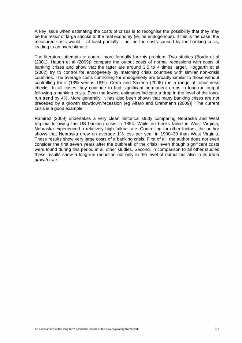
An assessment of the long-term economic impact of the new regulatory framework 37
A key issue when estimating the costs of crises is to recognise the possibility that they may be the result of large shocks to the real economy (ie, be endogenous). If this is the case, the measured costs would – at least partially – not be the costs caused by the banking crisis, leading to an overestimate.
The literature attempts to control more formally for this problem. Two studies (Bordo et al (2001), Haugh et al (2009)) compare the output costs of normal recessions with costs of banking crises and show that the latter are around 3.5 to 4 times larger. Hoggarth et al (2002) try to control for endogeneity by matching crisis countries with similar non-crisis countries. The average costs controlling for endogeneity are broadly similar to those without controlling for it (13% versus 16%). Cerra and Saxena (2008) run a range of robustness checks. In all cases they continue to find significant permanent drops in long-run output following a banking crisis. Even the lowest estimates indicate a drop in the level of the long-run trend by 4%. More generally, it has also been shown that many banking crises are not preceded by a growth slowdown/recession (eg Alfaro and Drehmann (2009)). The current crisis is a good example.
Ramirez (2009) undertakes a very clean historical study comparing Nebraska and West Virginia following the US banking crisis in 1894. While no banks failed in West Virginia, Nebraska experienced a relatively high failure rate. Controlling for other factors, the author shows that Nebraska grew on average 1% less per year in 1900–30 than West Virginia. These results show very large costs of a banking crisis. First of all, the author does not even consider the first seven years after the outbreak of the crisis, even though significant costs were found during this period in all other studies. Second, in comparison to all other studies these results show a long-run reduction not only in the level of output but also in its trend growth rate.
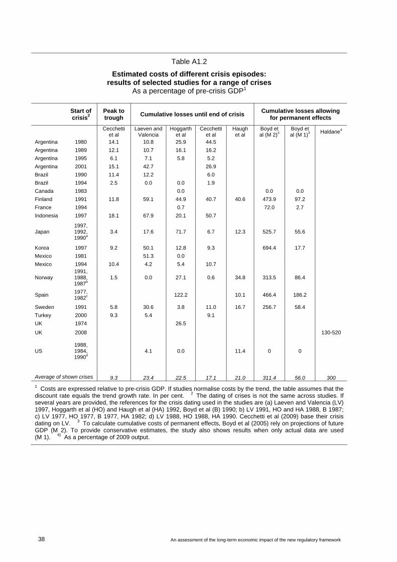
38 An assessment of the long-term economic impact of the new regulatory framework
Table A1.2
Estimated costs of different crisis episodes: results of selected studies for a range of crises
As a percentage of pre-crisis GDP1
Start of crisis2
Peak to trough
Cumulative losses until end of crisis Cumulative losses allowing
for permanent effects
Cecchetti
et al Laeven and
Valencia Hoggarth
et al Cecchetti
et al Haugh et al
Boyd et al (M 2)3
Boyd et al (M 1)3
Haldane4
Argentina 1980 14.1 10.8 25.9 44.5
Argentina 1989 12.1 10.7 16.1 16.2
Argentina 1995 6.1 7.1 5.8 5.2
Argentina 2001 15.1 42.7 26.9
Brazil 1990 11.4 12.2 6.0
Brazil 1994 2.5 0.0 0.0 1.9
Canada 1983 0.0 0.0 0.0
Finland 1991 11.8 59.1 44.9 40.7 40.6 473.9 97.2
France 1994 0.7 72.0 2.7
Indonesia 1997 18.1 67.9 20.1 50.7
Japan 1997, 1992, 1990a
3.4 17.6 71.7 6.7 12.3 525.7 55.6
Korea 1997 9.2 50.1 12.8 9.3 694.4 17.7
Mexico 1981 51.3 0.0
Mexico 1994 10.4 4.2 5.4 10.7
Norway 1991, 1988, 1987b
1.5 0.0 27.1 0.6 34.8 313.5 86.4
Spain 1977, 1982c
122.2 10.1 466.4 186.2
Sweden 1991 5.8 30.6 3.8 11.0 16.7 256.7 58.4
Turkey 2000 9.3 5.4 9.1
UK 1974 26.5
UK 2008 130-520
US 1988, 1984, 1990d
4.1 0.0 11.4 0 0
Average of shown crises 9.3 23.4 22.5 17.1 21.0 311.4 56.0 300 1 Costs are expressed relative to pre-crisis GDP. If studies normalise costs by the trend, the table assumes that the discount rate equals the trend growth rate. In per cent. 2 The dating of crises is not the same across studies. If several years are provided, the references for the crisis dating used in the studies are (a) Laeven and Valencia (LV) 1997, Hoggarth et al (HO) and Haugh et al (HA) 1992, Boyd et al (B) 1990; b) LV 1991, HO and HA 1988, B 1987; c) LV 1977, HO 1977, B 1977, HA 1982; d) LV 1988, HO 1988, HA 1990. Cecchetti et al (2009) base their crisis dating on LV. 3 To calculate cumulative costs of permanent effects, Boyd et al (2005) rely on projections of future GDP (M 2). To provide conservative estimates, the study also shows results when only actual data are used (M 1). 4) As a percentage of 2009 output.
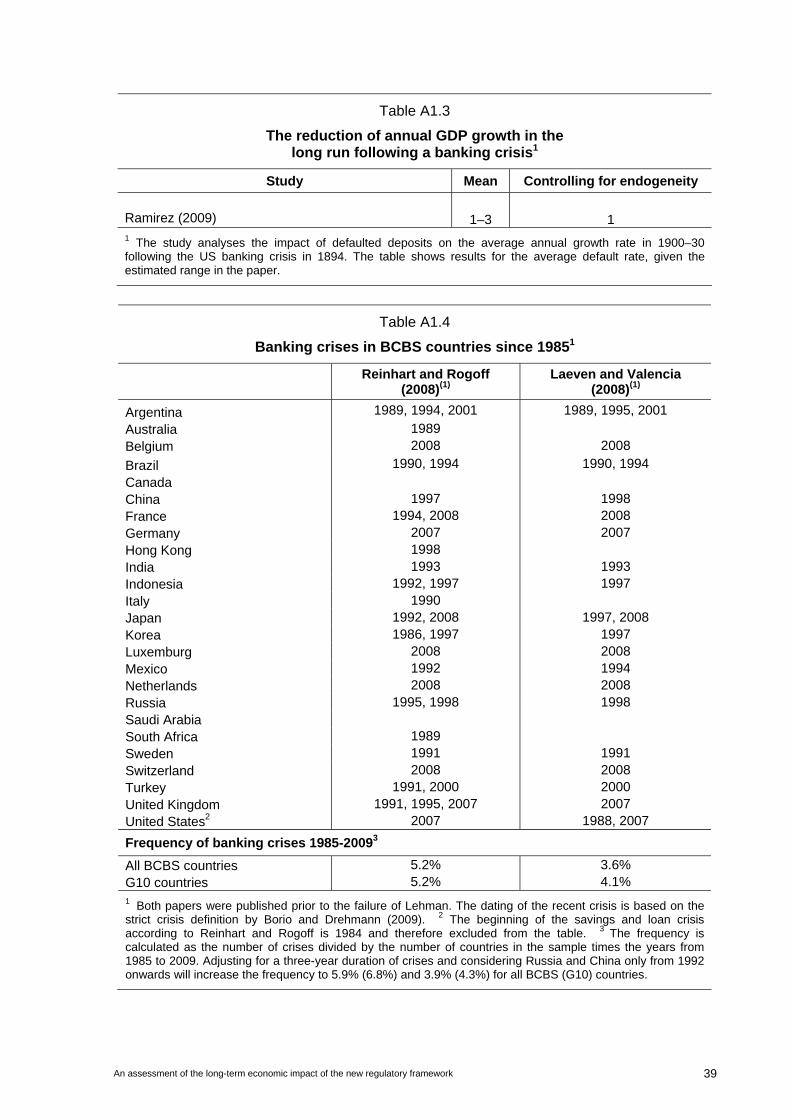
An assessment of the long-term economic impact of the new regulatory framework 39
Table A1.3
The reduction of annual GDP growth in the long run following a banking crisis1
Study Mean Controlling for endogeneity
Ramirez (2009) 1–3 1 1 The study analyses the impact of defaulted deposits on the average annual growth rate in 1900–30 following the US banking crisis in 1894. The table shows results for the average default rate, given the estimated range in the paper.
Table A1.4
Banking crises in BCBS countries since 19851
Reinhart and Rogoff
(2008)(1) Laeven and Valencia
(2008)(1)
Argentina 1989, 1994, 2001 1989, 1995, 2001
Australia 1989 Belgium 2008 2008
Brazil 1990, 1994 1990, 1994
Canada China 1997 1998 France 1994, 2008 2008 Germany 2007 2007 Hong Kong 1998 India 1993 1993 Indonesia 1992, 1997 1997 Italy 1990 Japan 1992, 2008 1997, 2008 Korea 1986, 1997 1997 Luxemburg 2008 2008 Mexico 1992 1994 Netherlands 2008 2008 Russia 1995, 1998 1998 Saudi Arabia South Africa 1989 Sweden 1991 1991 Switzerland 2008 2008 Turkey 1991, 2000 2000 United Kingdom 1991, 1995, 2007 2007 United States2 2007 1988, 2007
Frequency of banking crises 1985-20093
All BCBS countries 5.2% 3.6% G10 countries 5.2% 4.1% 1 Both papers were published prior to the failure of Lehman. The dating of the recent crisis is based on the strict crisis definition by Borio and Drehmann (2009). 2 The beginning of the savings and loan crisis according to Reinhart and Rogoff is 1984 and therefore excluded from the table. 3 The frequency is calculated as the number of crises divided by the number of countries in the sample times the years from 1985 to 2009. Adjusting for a three-year duration of crises and considering Russia and China only from 1992 onwards will increase the frequency to 5.9% (6.8%) and 3.9% (4.3%) for all BCBS (G10) countries.
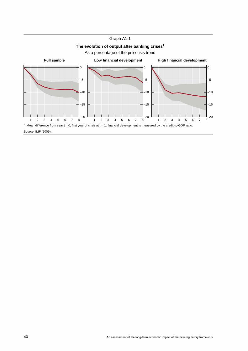
40 An assessment of the long-term economic impact of the new regulatory framework
Graph A1.1
The evolution of output after banking crises1
As a percentage of the pre-crisis trend
Full sample Low financial development High financial development
–20
–15
–10
–5
0
1 2 3 4 5 6 7 8
–20
–15
–10
–5
0
1 2 3 4 5 6 7 8–20
–15
–10
–5
0
1 2 3 4 5 6 7 81 Mean difference from year t = 0; first year of crisis at t = 1; financial development is measured by the credit-to-GDP ratio.
Source: IMF (2009).

An assessment of the long-term economic impact of the new regulatory framework 41
Annex 2
A brief summary of the crisis prediction/simulation models
This annex first provides methodological details of the models used to estimate the impact of tighter regulatory standards on the annual likelihood of a systemic banking crisis. It then discusses individual results.
Methodology
(i) FSA/NIESR model
Researchers at NIESR and the UK FSA (Barrell et al (2010b)) estimate a logit model explaining the probability of banking crises with the aggregate capital ratio, the aggregate liquidity ratio, the current account deficit and house price changes. Their sample includes annual data for 14 OECD countries from 1980 until 2008. And their sample of crises covers systemic and non-systemic crises from the World Bank (2003) crises database, updated for recent events. The final equation of the NIESR model is as follows:
)24.008.0_11.034.0()(Prob 2311 CbrRhpgLiqALevfcrises
Lev is the ratio of total capital over total assets, A_Liq is the ratio of cash and balances with the central bank plus securities over total assets, Rhpg is real house price growth, and Cbr is the ratio of the current account balance over nominal GDP. All the coefficients are statistically significant at least at the 5% level. Subscripts indicate time lags. As in other studies, the lags are included to limit the risk of reverse causality, ie that crises affect capital and liquidity rather than the other way round.
Results shown in Table A2.1 are based on setting the initial level of the liquidity ratio, the current account deficit and real house price growth at the respective mean across all countries in the sample for 2006. Ratios for TCE/RWA are mapped into the leverage ratio by following the methodology set out in Annex 5 and taking an average across European and US banks.
(ii) Bank of Japan model
Researchers from the Bank of Japan (Kato et al (2010)) estimate a probit model for 13 OECD countries, using annual data from 1980 to 2008. Crises cover both systemic and non-systemic crises, as identified in World Bank (2003) and Laeven and Valencia (2008). The authors estimate specifications with and without interactions among variables.
The final equation of the model without interactions is
)17.004._01.0_04.015.0()(Prob 22213 CbrRhpgLiqLLiqALevfcrises
and that of the model with interactions
)22.004.005.)_*(35.0)_*(96.0()(Prob 2222313 CbrDRhpRhpgLiqLLevLiqALevfcrises
42 An assessment of the long-term economic impact of the new regulatory framework
Lev is the ratio of total capital over total assets, A_Liq is the ratio of cash and balances with the central bank plus securities over total assets, L_Liq is the ratio of customer deposits to total deposits, and Rhpg is real house price growth. Cbr is the ratio of the current account balance to nominal GDP. All the coefficients are statistically significant in both specification at least at the 5% level. Subscripts indicate time lags.
Results shown in Table A2.1 are based on setting the initial level of the liquidity ratios, the current account deficit and real house price growth at the respective mean across all countries in the sample for 2006. Ratios for TCE/RWA are mapped into the leverage ratio by following the methodology set out in Annex 5 and taking an average across European and US banks.
(iii) The estimated portfolio model
As with other portfolio models (see below), this approach calculates the probability of a systemic crisis by interpreting the banking system as a portfolio of banks (the analogue of individual securities for portfolio credit risk models). For this report, it is assumed that systemic risk materialises when four or more institutions fail. Default correlations are based on Moody’s KMV estimates of the institutions’ asset-return correlations in order to derive the sensitivity of banks’ assets to common shocks. The model is estimated for the 51 largest banks globally and shocks are assumed to follow a normal distribution.
Bank-specific probabilities of default (PDs) in the estimated portfolio model are based on a simple logit model linking capital and liquidity ratios to the likelihood of default. The logit model is estimated for a sample of over 110 large globally active banks – including the 51 banks considered in the final model – using data from 2000 until 2008. The identification of stressed banks is based on input from national supervisors. A range of models has been estimated, dropping various countries or including other control variables. But the results for the leverage and liquidity ratio are very robust. For the simulations shown in this paper we use the following specification
PD(bank)=f(-0.5-50*Cap-1 -3*L_Liq-1)
where Cap is the ratio of TCE to total assets and L_Liq the ratio of customer deposits to total liabilities. All the coefficients are statistically significant at least at the 5% level.44
Results shown in Table A2.1 are based on setting the liquidity ratio at the end-2006 level for individual banks. Correlations are based on end-2007 data. Ratios for TCE/RWA are mapped into the ratio of TCE over total assets by following the methodology set out in Annex 5 and taking an average across European and US banks.
(iv) Bank of England Merton-style model
In order to quantify the link between the banking sector’s capitalisation and the likelihood of a systemic banking crisis, researchers at the Bank of England used a Merton-style structural credit risk model based on Elsinger et al (2006). The framework captures two channels of system-wide risk: (i) the risk that banks fail simultaneously, because their asset values are
44 The ratio of liquid assets to total assets was also incorporated in some estimations but found to be
insignificant.
An assessment of the long-term economic impact of the new regulatory framework 43
correlated; and (ii) direct balance sheet links between banks, through which the failure of one bank can cause the failure of other institutions.
The model is calibrated using data for the five largest UK banks, with a systemic crisis defined as the joint default of at least two of these banks. Following Merton (1974), the volatility and the covariance of each bank’s assets is inferred from the volatility of the market value of its equity. The results are sensitive to the period over which it is calibrated. The more volatile equity prices over the period, the greater the inferred volatility of the bank’s assets, and the greater the chance that the asset value falls sufficiently to push a bank’s equity below the threshold for failure. The reported results allow for some uncertainty in this viability threshold.
(v) BIS model
The BIS model is a variant of a model developed by Tarashev and Zhu (2008). It interprets the banking system as a portfolio of banks and estimates the loss distribution arising from bank defaults. Bank failures are correlated. Correlations are based on Moody’s KMV estimate of the institutions’ asset-return correlations. In contrast to the BoE model and the baseline version of Tarashev and Zhu, which assume that shocks to banks’ assets are normally distributed, the model assumes a T distribution with four degrees of freedom. This distribution has fatter tails. The model is estimated for the 51 largest banks globally. Correlations are based on end-2007 data. For this report it is assumed that systemic risk materialises when four or more institutions fail. Ratios for TCE/RWA are mapped into the ratio of shareholder equity over total assets following the methodology set out in Annex 5 for European banks.
When simulating the impact of higher capital levels on the probability of systemic crises, the BoE and BIS models hold all other parameters, including the volatility of assets, constant. If banks, however, take on more risk to compensate for higher capital requirements, this would tend to reduce the marginal impact on the probability of failure of individual institutions and hence of systemic risk.
(vi) The Bank of Canada stress testing framework
The simulations in this report use the stress testing model developed by researchers at the Bank of Canada. Details about the model and data are provided by Gauthier et al (2010). The authors look at six major Canadian banks for the period ending Q2 2008. The model generates the distribution of credit losses at Canadian banks under a severe but plausible scenario. It incorporates the impact of externalities through counterparty credit risk and asset fire sales. Asset fire sales are triggered whenever the Tier 1 capital ratio of a bank falls below 7% (the minimum required by the Canadian regulator). In case of an asset fire sale, the equilibrium price for illiquid assets is obtained from a calibrated demand curve and the endogenous aggregate supply of assets. Contagion occurs through counterparty credit risk and mark to market accounting as in Cifuentes et al (2005).
44 An assessment of the long-term economic impact of the new regulatory framework
Results
Table A2.1 shows simulation results for each model for different capital and liquidity ratios. Table A2.2 summarises this information by looking at average results for different modelling approaches.45 This table in turn provides the basis for results used in the main text (Table 3). The summary results do not include the stress testing exercise conducted by the Bank of Canada. The fact that these results reflect the links between liquidity, capital and crisis under stressful scenarios sets them apart from the results of models that are more geared to average relationships. Had the stress testing results been included in the averages reported in Table A2.2 the conclusions would have been qualitatively identical but the marginal impact of liquidity would have been smaller.
The simulations of the reduced-form models indicate an average probability of a systemic crisis of 4.1% when the capital ratio is 7% and there is no change in any of the liquidity ratios from their pre-crisis levels. This is at the low end of the historical average of 4–5%.Within the framework of these models, increasing capital ratios by 1 percentage point reduces the annual probability of systemic crises by around 25–30%, depending on the starting level of capital. For example, the reduction in the probability is from 4.1% to 2.8% when capital is increased from 7% to 8%. Meeting the NSFR, as modelled by a 12.5% increase in the ratio of liquid assets over total assets (see Annex 5 for a detailed discussion of the mapping between meeting the NSFR and the liquidity ratios used by the reduced-form models), has a somewhat lower effect as it reduces the annual probability of crisis by around 15–20%. Increasing the liquid asset ratio by 25% or even 50% has clearly a larger impact on the likelihood of systemic crises.
The two reduced-form models estimated by researchers from the Bank of Japan also incorporate the ratio of deposits relative to total liabilities as another liquidity ratio. Using these models shows that increasing the ratio of deposits to total assets by 10 percentage points (one way of increasing funding liquidity) reduces the probability of crises by around one sixth (eg 4.1% to 2.9% for a 7% TCE/RWA ratio).46 A 20 percentage point increase would lower the probability by more than one third (eg 4.1% to 2.4% for a 7% TCE/RWA ratio).
The second panel of Table A2.2 reports average results based on portfolio credit risk models. The results of these three models are similar to those coming from the reduced-form approaches. For instance, increasing the ratio of TCE to RWA from 7% to 8% reduces the probability of crisis by roughly one third (eg 5.1% to 3.1%), with no change in liquidity. Increases in the ratio of deposits to total liabilities also serve to reduce the probability of a crisis. But this is only captured by one model.
The last panel in Table A2.1 reports the impact of liquidity and capital ratios on the likelihood that two or more banks default, conditional on a very severe macroeconomic shock. In this environment, higher capital ratios clearly have large benefits. Increasing capital ratios from 7% to 8% decreases the likelihood of a systemic crisis by two thirds (eg from 4.7% to 1.7%) with no increase in liquidity. By design, the role of liquidity is limited in the stress test model. Nonetheless, higher liquidity buffers are still found to yield a modest benefit. For example, when the capital ratio is 7%, increasing the ratio of liquid assets by 25% reduces the likelihood of crisis by around 0.1 percentage points (eg from 4.7% to 4.6%).
45 Given the small number of models the average rather than median is presented. However, using all models
the average and median are very similar. 46 Results shown in Table A2.2 indicate a different impact as the average for “no increase in liquidity” also
incorporates the FSA model.
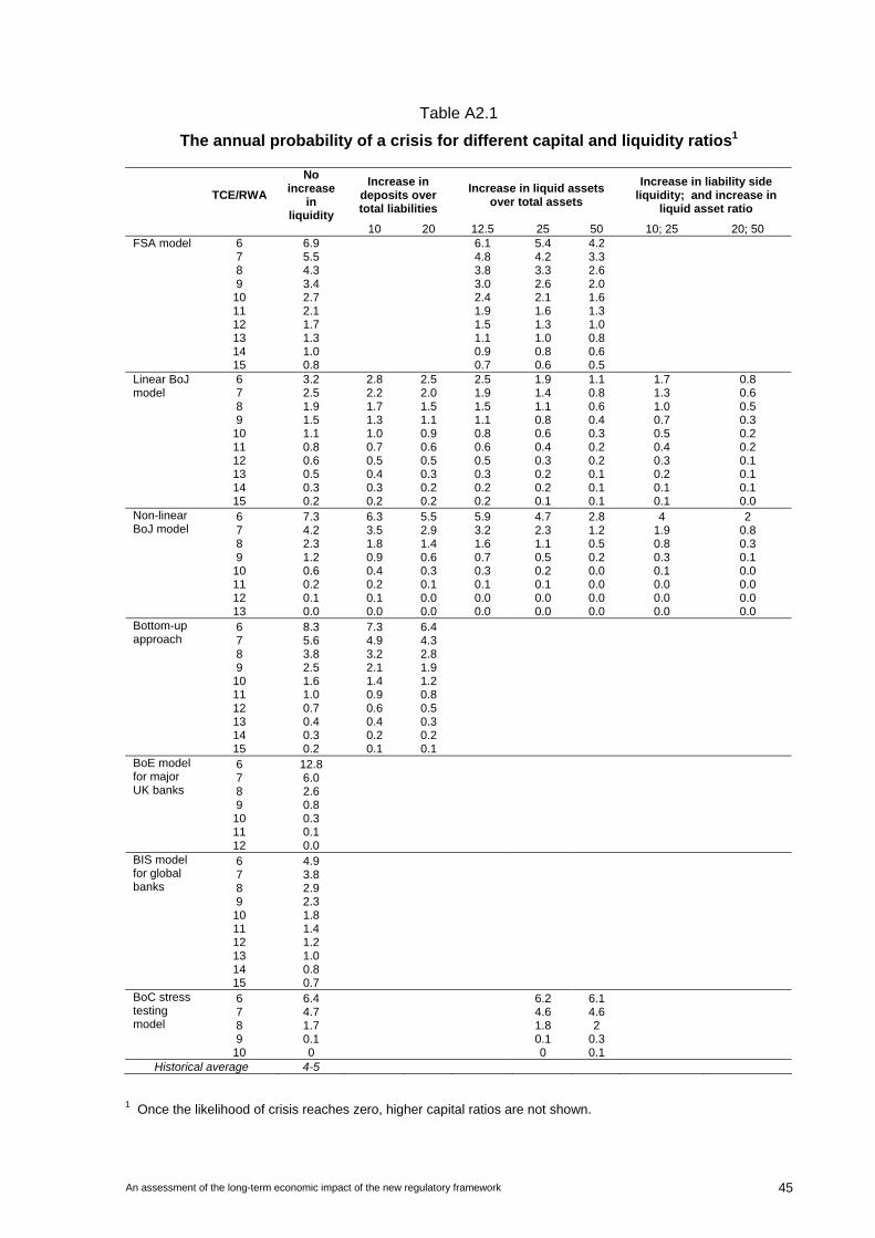
An assessment of the long-term economic impact of the new regulatory framework 45
Table A2.1
The annual probability of a crisis for different capital and liquidity ratios1
TCE/RWA
No increase
in liquidity
Increase in deposits over total liabilities
Increase in liquid assets over total assets
Increase in liability side liquidity; and increase in
liquid asset ratio
10 20 12.5 25 50 10; 25 20; 50 6 6.9 6.1 5.4 4.2 7 5.5 4.8 4.2 3.3 8 4.3 3.8 3.3 2.6
FSA model
9 3.4 3.0 2.6 2.0 10 2.7 2.4 2.1 1.6 11 2.1 1.9 1.6 1.3 12 1.7 1.5 1.3 1.0 13 1.3 1.1 1.0 0.8 14 1.0 0.9 0.8 0.6 15 0.8 0.7 0.6 0.5
6 3.2 2.8 2.5 2.5 1.9 1.1 1.7 0.8 7 2.5 2.2 2.0 1.9 1.4 0.8 1.3 0.6 8 1.9 1.7 1.5 1.5 1.1 0.6 1.0 0.5 9 1.5 1.3 1.1 1.1 0.8 0.4 0.7 0.3
Linear BoJ model
10 1.1 1.0 0.9 0.8 0.6 0.3 0.5 0.2 11 0.8 0.7 0.6 0.6 0.4 0.2 0.4 0.2 12 0.6 0.5 0.5 0.5 0.3 0.2 0.3 0.1 13 0.5 0.4 0.3 0.3 0.2 0.1 0.2 0.1 14 0.3 0.3 0.2 0.2 0.2 0.1 0.1 0.1 15 0.2 0.2 0.2 0.2 0.1 0.1 0.1 0.0
6 7.3 6.3 5.5 5.9 4.7 2.8 4 2 7 4.2 3.5 2.9 3.2 2.3 1.2 1.9 0.8 8 2.3 1.8 1.4 1.6 1.1 0.5 0.8 0.3 9 1.2 0.9 0.6 0.7 0.5 0.2 0.3 0.1
Non-linear BoJ model
10 0.6 0.4 0.3 0.3 0.2 0.0 0.1 0.0 11 0.2 0.2 0.1 0.1 0.1 0.0 0.0 0.0 12 0.1 0.1 0.0 0.0 0.0 0.0 0.0 0.0 13 0.0 0.0 0.0 0.0 0.0 0.0 0.0 0.0
6 8.3 7.3 6.4 7 5.6 4.9 4.3 8 3.8 3.2 2.8 9 2.5 2.1 1.9
10 1.6 1.4 1.2
Bottom-up approach
11 1.0 0.9 0.8 12 0.7 0.6 0.5 13 0.4 0.4 0.3 14 0.3 0.2 0.2 15 0.2 0.1 0.1
6 12.8 7 6.0 8 2.6
BoE model for major UK banks
9 0.8 10 0.3 11 0.1 12 0.0
6 4.9 7 3.8 8 2.9 9 2.3
BIS model for global banks
10 1.8 11 1.4 12 1.2 13 1.0 14 0.8 15 0.7
6 6.4 6.2 6.1 7 4.7 4.6 4.6 8 1.7 1.8 2 9 0.1 0.1 0.3
BoC stress testing model
10 0 0 0.1 Historical average 4-5
1 Once the likelihood of crisis reaches zero, higher capital ratios are not shown.
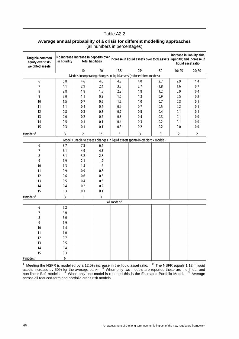
46 An assessment of the long-term economic impact of the new regulatory framework
Table A2.2
Average annual probability of a crisis for different modelling approaches (all numbers in percentages)
No increase in liquidity
Increase in deposits over total liabilities Increase in liquid assets over total assets
Increase in liability side liquidity; and increase in
liquid asset ratio
Tangible common equity over risk-weighted assets
10 20 12.51 252 50 10; 25 20; 50 Models incorporating changes in liquid assets (reduced-form models)
6 5.8 4.6 4.0 4.8 4.0 2.7 2.9 1.4 7 4.1 2.9 2.4 3.3 2.7 1.8 1.6 0.7 8 2.8 1.8 1.5 2.3 1.8 1.2 0.9 0.4 9 2.0 1.1 0.9 1.6 1.3 0.9 0.5 0.2 10 1.5 0.7 0.6 1.2 1.0 0.7 0.3 0.1 11 1.1 0.4 0.4 0.9 0.7 0.5 0.2 0.1 12 0.8 0.3 0.3 0.7 0.5 0.4 0.1 0.1 13 0.6 0.2 0.2 0.5 0.4 0.3 0.1 0.0 14 0.5 0.1 0.1 0.4 0.3 0.2 0.1 0.0 15 0.3 0.1 0.1 0.3 0.2 0.2 0.0 0.0
# models3 3 2 2 3 3 3 2 2
Models unable to assess changes in liquid assets (portfolio credit risk models)
6 8.7 7.3 6.4 7 5.1 4.9 4.3 8 3.1 3.2 2.8 9 1.9 2.1 1.9 10 1.3 1.4 1.2 11 0.9 0.9 0.8 12 0.6 0.6 0.5 13 0.5 0.4 0.3 14 0.4 0.2 0.2 15 0.3 0.1 0.1
# models4 3 1 1 All models5
6 7.2 7 4.6 8 3.0 9 1.9 10 1.4 11 1.0 12 0.7 13 0.5 14 0.4 15 0.3
# models 6
1 Meeting the NSFR is modelled by a 12.5% increase in the liquid asset ratio. 2 The NSFR equals 1.12 if liquid assets increase by 50% for the average bank. 3 When only two models are reported these are the linear and non-linear BoJ models. 4 When only one model is reported this is the Estimated Portfolio Model. 5 Average across all reduced-form and portfolio credit risk models.
An assessment of the long-term economic impact of the new regulatory framework 47
Annex 3
Mapping higher capital and liquidity requirements to lending spreads
This annex provides details on how the increased cost of higher capital and liquidity requirements are mapped to higher lending spreads. The calculations are based on a representative bank for each country, with the results averaged across countries to arrive at the estimates reported in Table 7. The calculation assumes that the ROE and cost of debt do not change with lower leverage. It also assumes that banks pass on any additional costs to lending spreads, and do not adjust other sources of income or operating expenses. For each country, the impact on lending spreads is calculated (i) assuming no change in RWA, and (ii) allowing RWA to decline as steps are taken to meet the NSFR (namely holding more government bonds relative to other investments). Within each scenario, the costs are calculated for incremental increases in capital ratios of 1 percentage point. These costs are linear in the increase in capital ratios.
The exercise is conducted as follows. A representative bank for each country is constructed based on aggregate banking sector data for 13 OECD countries. Income statement and balance sheet data from 6,600 banks are averaged over the 15-year period from 1993 to 2007. These representative banks proxy for a long-run average or “steady state” reflecting each country’s institutional setting and regulatory framework. All variables are standardised by dividing by a bank’s total assets in a given year.
Table A3.1 shows the stylised balance sheet and income statement based on the simple average of the representative figures for each of the 13 countries. All items are shown as a percentage of total assets. Loans represent about half of the typical banks’ assets, followed by investments (16.1%), interbank claims (12.2%) and trading-related assets (10.4%). These assets are funded primarily by deposits (43.5%), trading-related liabilities (15.2%), debt (14.2%) and interbank funding (12.6%). Shareholders’ equity represents 5.3% of assets, of which common equity is the majority (4.7%). Risk-weighted assets represent around half of total assets.
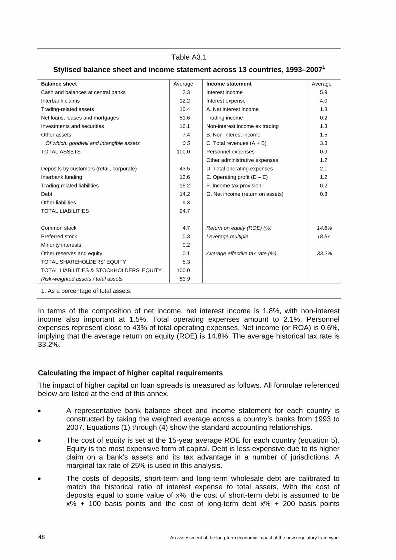
48 An assessment of the long-term economic impact of the new regulatory framework
Table A3.1
Stylised balance sheet and income statement across 13 countries, 1993–20071
Balance sheet Average Income statement Average
Cash and balances at central banks 2.3 Interest income 5.9
Interbank claims 12.2 Interest expense 4.0
Trading-related assets 10.4 A. Net interest income 1.8
Net loans, leases and mortgages 51.6 Trading income 0.2
Investments and securities 16.1 Non-interest income ex trading 1.3
Other assets 7.4 B. Non-interest income 1.5
Of which: goodwill and intangible assets 0.5 C. Total revenues (A + B) 3.3
TOTAL ASSETS 100.0 Personnel expenses 0.9
Other administrative expenses 1.2
Deposits by customers (retail, corporate) 43.5 D. Total operating expenses 2.1
Interbank funding 12.6 E. Operating profit (D – E) 1.2
Trading-related liabilities 15.2 F. Income tax provision 0.2
Debt 14.2 G. Net income (return on assets) 0.8
Other liabilities 9.3
TOTAL LIABILITIES 94.7
Common stock 4.7 Return on equity (ROE) (%) 14.8% Preferred stock 0.3 Leverage multiple 18.5x Minority interests 0.2 Other reserves and equity 0.1 Average effective tax rate (%) 33.2% TOTAL SHAREHOLDERS’ EQUITY 5.3 TOTAL LIABILITIES & STOCKHOLDERS' EQUITY 100.0 Risk-weighted assets / total assets 53.9
1. As a percentage of total assets.
In terms of the composition of net income, net interest income is 1.8%, with non-interest income also important at 1.5%. Total operating expenses amount to 2.1%. Personnel expenses represent close to 43% of total operating expenses. Net income (or ROA) is 0.6%, implying that the average return on equity (ROE) is 14.8%. The average historical tax rate is 33.2%.
Calculating the impact of higher capital requirements
The impact of higher capital on loan spreads is measured as follows. All formulae referenced below are listed at the end of this annex.
A representative bank balance sheet and income statement for each country is constructed by taking the weighted average across a country’s banks from 1993 to 2007. Equations (1) through (4) show the standard accounting relationships.
The cost of equity is set at the 15-year average ROE for each country (equation 5). Equity is the most expensive form of capital. Debt is less expensive due to its higher claim on a bank’s assets and its tax advantage in a number of jurisdictions. A marginal tax rate of 25% is used in this analysis.
The costs of deposits, short-term and long-term wholesale debt are calibrated to match the historical ratio of interest expense to total assets. With the cost of deposits equal to some value of x%, the cost of short-term debt is assumed to be x% + 100 basis points and the cost of long-term debt x% + 200 basis points
An assessment of the long-term economic impact of the new regulatory framework 49
(equations 6 to 8). These spreads are consistent with historical averages across the countries in this sample, and generate an upward-sloping yield curve. The share of debt that is less than one year in maturity (rho) is set at 25% (equation 10). Interest expense is then calculated using equation (11).
Interest income is generated by interbank claims, loans and investments. Trading income is generated by trading assets minus trading liabilities. A portion of investments (theta) is invested in government bonds that return a risk-free rate of interest, while the remaining investments are invested in higher-yielding securities. The risk premium on these higher-yielding investments is the difference between the return on investments and the risk-free rate (equation 9).
From this starting point, the quantity of TCE/RWA is increased by increments of 1 percentage point to meet specific targets of RWA (equation 14). The size and composition of the balance sheet is held constant but the relative share financed by equity and debt changes.
An increase of TCE/RWA of 1 percentage point generates a smaller rise in equity as RWA are typically only 50% of total assets (equation 15). This increase in the quantity of equity is matched by a decrease in the quantity of debt (equation 16). As the most expensive form of debt, long-term debt is the first to be replaced with equity.
The change in capital structure leads to a rise in the bank’s cost of capital, as tax-advantaged debt is substituted with more expensive equity. A higher quantity of equity for a given level of net income leads to a fall in ROE (equation 5). Part of this fall in ROE is offset by the decline in interest expense due to the smaller quantity of debt outstanding (equations 11 and 16).
In the central scenario, it is assumed that the cost of equity and the cost of long-term debt are unchanged. In theory, the cost of equity and debt should both decline as leverage decreases and the risk of default becomes smaller. The estimates in this analysis therefore are conservative, as a fall in either of these costs would reduce the impact on loan spreads.
Banks respond to the fall in ROE by raising the spreads charged on loans (alpha, equation 17). The size of the increase in loan spreads is determined such that the increase in net income exactly offsets the increase in the cost of capital, allowing ROE to be unchanged (equation 18).
Calculating the cost to meet the December 2009 proposal for the NSFR
The formula for calculating the NSFR is detailed in the December 2009 BCBS consultative document, with a simplified version shown in equation 19. The numerator measures the sources of available stable funding (ASF), with greater weight given to funding sources that are more stable and least likely to disappear under stressed market conditions. Equity, longer-term debt and longer-term liabilities are the most stable forms of funding, followed by deposits. The denominator shows assets that require funding, with a factor (or haircut) applied based on their expected liquidation value under stressed circumstances. Cash, securities with less than one year to maturity and interbank loans do not have to be funded and have a factor of 0%. Government debt is considered very liquid and must only be funded at 5% of face value. Corporate loans and retail loans that mature within one year must be funded 50% and 85%, respectively, assuming that they are not rolled over when they mature. All remaining assets must be funded at 100%. To achieve a target NSFR, banks must extend the maturity of their funding and reduce the maturity or the riskiness of their assets.
50 An assessment of the long-term economic impact of the new regulatory framework
An estimate of the impact of the NSFR requires details on the composition of investments held by banks, the stability of their deposits, and the size of “Other assets”. This information is not available, but is being collected by the BCBS through the Quantitative Impact Study (QIS). In the absence of QIS data, the only way to arrive at a starting value of the NSFR is to make a number of assumptions. Supervisors in some countries provided rough estimates for their banks, and these estimates are applied to all the sample countries as follows:
75% of deposits are stable
25% of securities are less than 1 year in maturity
25% of corporate loans are less than 1 year in maturity
25% of retail loans are less than 1 year in maturity
25% debt is less than 1 year in maturity
government debt initially makes up 25% of investments
The calculation of the cost to meet the NSFR is very sensitive to these assumptions, as well as the relative size of these categories on banks’ balance sheets.
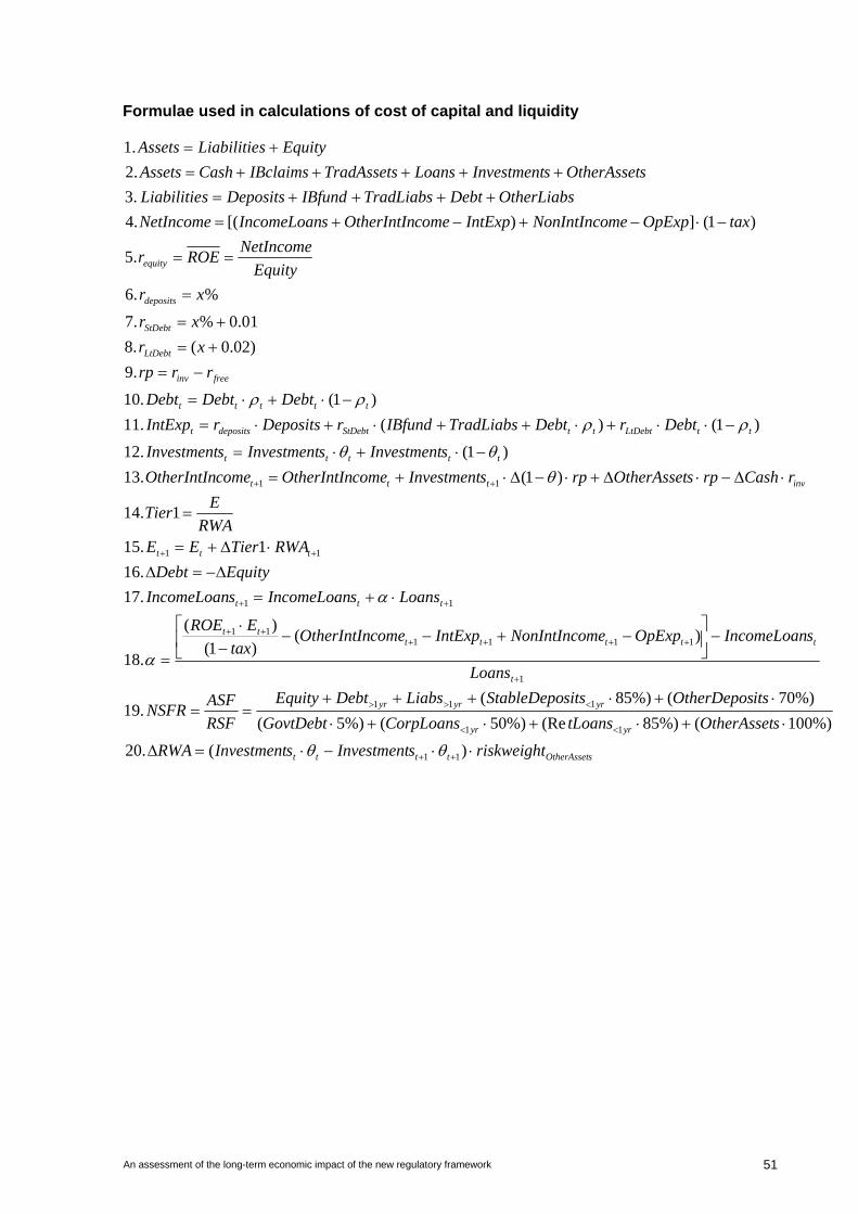
An assessment of the long-term economic impact of the new regulatory framework 51
Formulae used in calculations of cost of capital and liquidity
sOtherAssettttt
yryr
yryryr
t
ttttttt
ttt
ttt
invttt
ttttt
ttLtDebtttStDebtdepositst
ttttt
freeinv
LtDebt
StDebt
deposits
equity
riskweightsInvestmentsInvestmentRWA
sOtherAssettLoansCorpLoansGovtDebt
itsOtherDepossitsStableDepoLiabsDebtEquity
RSF
ASFNSFR
Loans
sIncomeLoanOpExpmeNonIntIncoIntExpcomeOtherIntIntax
EROE
LoanssIncomeLoansIncomeLoan
EquityDebt
RWATierEERWA
ETier
rCashrpsOtherAssetrpsInvestmentcomeOtherIntIncomeOtherIntIn
sInvestmentsInvestmentsInvestment
DebtrDebtTradLiabsIBfundrDepositsrIntExp
DebtDebtDebt
rrrp
xr
xr
xr
Equity
NetIncomeROEr
taxOpExpmeNonIntIncoIntExpcomeOtherIntInsIncomeLoanNetIncome
OtherLiabsDebtTradLiabsIBfundDepositssLiabilitie
sOtherAssetsInvestmentLoansTradAssetsIBclaimsCashAssets
EquitysLiabilitieAssets
)(.20
%)100(%)85(Re%)50(%)5(
%)70(%)85(.19
)()1(
)(
.18
.17
.16
1.15
1.14
)1(.13
)1(.12
)1()(.11
)1(.10
.9
)02.0(.8
01.0%.7
%.6
.5
)1(])[(.4
.3
.2
.1
11
11
111
1
111111
11
11
11
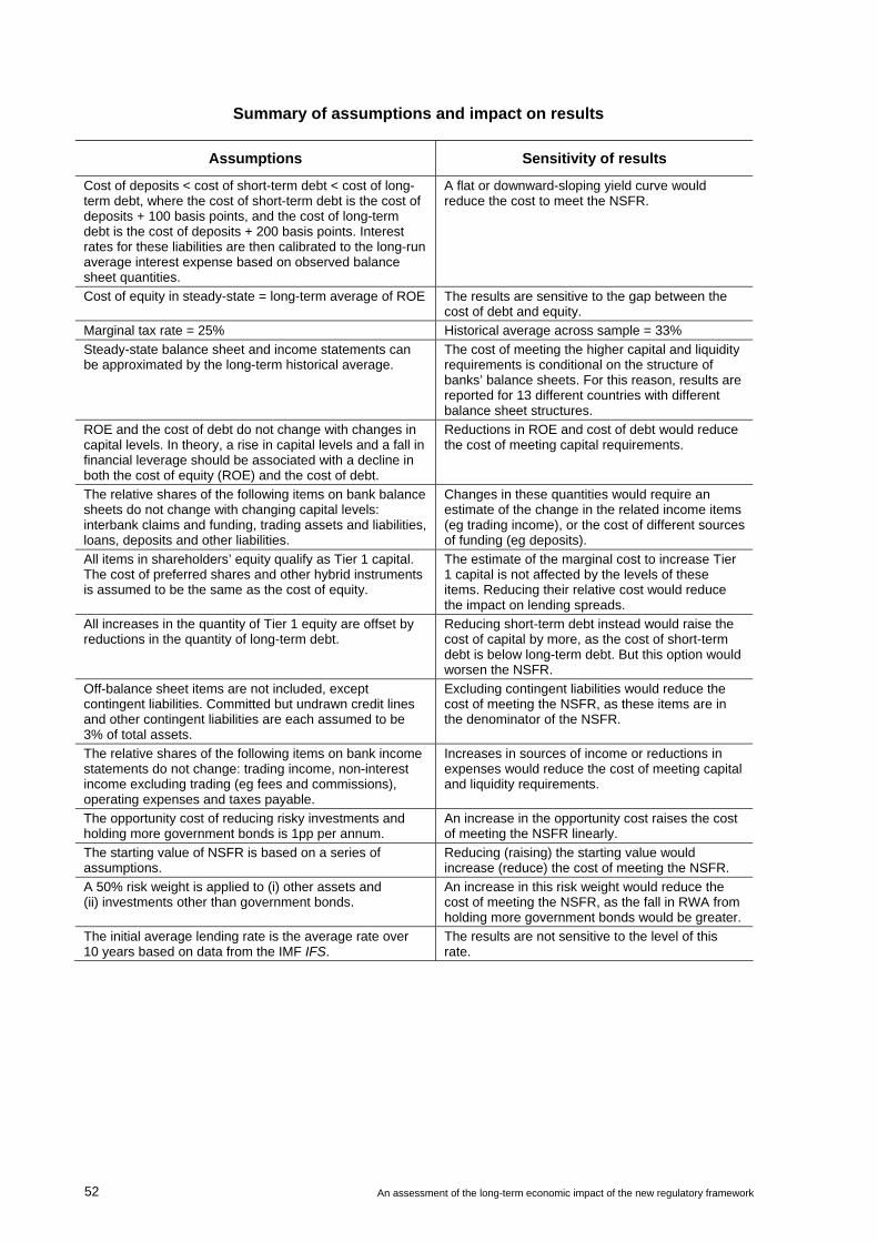
52 An assessment of the long-term economic impact of the new regulatory framework
Summary of assumptions and impact on results
Assumptions Sensitivity of results
Cost of deposits < cost of short-term debt < cost of long-term debt, where the cost of short-term debt is the cost of deposits + 100 basis points, and the cost of long-term debt is the cost of deposits + 200 basis points. Interest rates for these liabilities are then calibrated to the long-run average interest expense based on observed balance sheet quantities.
A flat or downward-sloping yield curve would reduce the cost to meet the NSFR.
Cost of equity in steady-state = long-term average of ROE The results are sensitive to the gap between the cost of debt and equity.
Marginal tax rate = 25% Historical average across sample = 33%
Steady-state balance sheet and income statements can be approximated by the long-term historical average.
The cost of meeting the higher capital and liquidity requirements is conditional on the structure of banks’ balance sheets. For this reason, results are reported for 13 different countries with different balance sheet structures.
ROE and the cost of debt do not change with changes in capital levels. In theory, a rise in capital levels and a fall in financial leverage should be associated with a decline in both the cost of equity (ROE) and the cost of debt.
Reductions in ROE and cost of debt would reduce the cost of meeting capital requirements.
The relative shares of the following items on bank balance sheets do not change with changing capital levels: interbank claims and funding, trading assets and liabilities, loans, deposits and other liabilities.
Changes in these quantities would require an estimate of the change in the related income items (eg trading income), or the cost of different sources of funding (eg deposits).
All items in shareholders’ equity qualify as Tier 1 capital. The cost of preferred shares and other hybrid instruments is assumed to be the same as the cost of equity.
The estimate of the marginal cost to increase Tier 1 capital is not affected by the levels of these items. Reducing their relative cost would reduce the impact on lending spreads.
All increases in the quantity of Tier 1 equity are offset by reductions in the quantity of long-term debt.
Reducing short-term debt instead would raise the cost of capital by more, as the cost of short-term debt is below long-term debt. But this option would worsen the NSFR.
Off-balance sheet items are not included, except contingent liabilities. Committed but undrawn credit lines and other contingent liabilities are each assumed to be 3% of total assets.
Excluding contingent liabilities would reduce the cost of meeting the NSFR, as these items are in the denominator of the NSFR.
The relative shares of the following items on bank income statements do not change: trading income, non-interest income excluding trading (eg fees and commissions), operating expenses and taxes payable.
Increases in sources of income or reductions in expenses would reduce the cost of meeting capital and liquidity requirements.
The opportunity cost of reducing risky investments and holding more government bonds is 1pp per annum.
An increase in the opportunity cost raises the cost of meeting the NSFR linearly.
The starting value of NSFR is based on a series of assumptions.
Reducing (raising) the starting value would increase (reduce) the cost of meeting the NSFR.
A 50% risk weight is applied to (i) other assets and (ii) investments other than government bonds.
An increase in this risk weight would reduce the cost of meeting the NSFR, as the fall in RWA from holding more government bonds would be greater.
The initial average lending rate is the average rate over 10 years based on data from the IMF IFS.
The results are not sensitive to the level of this rate.
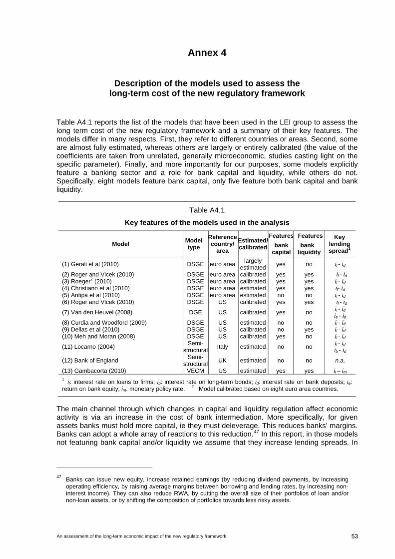
An assessment of the long-term economic impact of the new regulatory framework 53
Annex 4
Description of the models used to assess the long-term cost of the new regulatory framework
Table A4.1 reports the list of the models that have been used in the LEI group to assess the long term cost of the new regulatory framework and a summary of their key features. The models differ in many respects. First, they refer to different countries or areas. Second, some are almost fully estimated, whereas others are largely or entirely calibrated (the value of the coefficients are taken from unrelated, generally microeconomic, studies casting light on the specific parameter). Finally, and more importantly for our purposes, some models explicitly feature a banking sector and a role for bank capital and liquidity, while others do not. Specifically, eight models feature bank capital, only five feature both bank capital and bank liquidity.
Table A4.1
Key features of the models used in the analysis
Model Model type
Referencecountry/
area
Estimated/calibrated
Features
bank capital
Features
bank liquidity
Key lending spread1
(1) Gerali et al (2010) DSGE euro arealargely
estimatedyes no il - id
(2) Roger and Vlcek (2010) DSGE euro area calibrated yes yes il - id (3) Roeger2 (2010) DSGE euro area calibrated yes yes il - id (4) Christiano et al (2010) DSGE euro area estimated yes yes il- id (5) Antipa et al (2010) DSGE euro area estimated no no il - id (6) Roger and Vlcek (2010) DSGE US calibrated yes yes il - id
(7) Van den Heuvel (2008) DGE US calibrated yes no il - id ie - id
(8) Curdia and Woodford (2009) DSGE US estimated no no il - id (9) Dellas et al (2010) DSGE US calibrated no yes il - id (10) Meh and Moran (2008) DSGE US calibrated yes no il - id
(11) Locarno (2004) Semi-
structuralItaly estimated no no
il - id ib - id
(12) Bank of England Semi-
structuralUK estimated no no n.a.
(13) Gambacorta (2010) VECM US estimated yes yes il – im 1 il: interest rate on loans to firms; ib: interest rate on long-term bonds; id: interest rate on bank deposits; ie: return on bank equity; im: monetary policy rate. 2 Model calibrated based on eight euro area countries.
The main channel through which changes in capital and liquidity regulation affect economic activity is via an increase in the cost of bank intermediation. More specifically, for given assets banks must hold more capital, ie they must deleverage. This reduces banks’ margins. Banks can adopt a whole array of reactions to this reduction.47 In this report, in those models not featuring bank capital and/or liquidity we assume that they increase lending spreads. In
47 Banks can issue new equity, increase retained earnings (by reducing dividend payments, by increasing
operating efficiency, by raising average margins between borrowing and lending rates, by increasing non-interest income). They can also reduce RWA, by cutting the overall size of their portfolios of loan and/or non-loan assets, or by shifting the composition of portfolios towards less risky assets.
54 An assessment of the long-term economic impact of the new regulatory framework
the models in which bank capital and/or liquidity are explicitly modelled, the increase in lending spreads arises endogenously as the response to the new regulation. Owing to imperfect substitutability between bank credit and other forms of market financing (such as bonds), this leads to lower investment and consumption, which then affects employment and output.
The reduction of investment activity induces a one-off loss of output in the long run as the marginal product of capital has to rise in line with the lending rate spreads. Over the long run monetary policy is assumed to be neutral.48 By contrast, the short-term monetary policy reaction is important to assess the effect of the new regulation on output variability (see Section II.B).
Most of the models used in the simulations carried out specifically for this exercise belong to the Dynamic Stochastic General Equilibrium (DSGE) family. These models have a number of advantages for the purpose at hand. By choice, most of the models feature banks’ balance sheets and credit markets explicitly. This permits us to analyse in a unified framework how changes in capital and liquidity requirements affect banking conditions (spreads and lending) and ultimately output. In addition, DSGE models allow counterfactual policy experiments in a conceptually consistent manner. As agents’ expectations are explicitly modelled, so is their reaction to the simulated policy change. Finally, DSGE models allow us to study the effect of the policy changes not only on the steady-state values of the key macroeconomic variables, but also on their long-term variability. That said, DSGE models have disadvantages too. Many of the available models are fully or partially calibrated, since estimation is often daunting. As a result, quantitative results from some of these models might be questionable. And the variants used here are still experimental, so that they are not fully integrated in the policy-making process.
In a few cases it has been possible to use semi-structural models. Most central banks and many other economic agencies have one or more, regularly updated, macroeconomic models that have demonstrated their usefulness over time for forecasting and policy analysis. For the most part, however, these models do not directly incorporate balance sheet conditions and income statements of banks as input variables. Instead, these effects must be incorporated into other variables, such as lending spreads. This means that the first step of the transmission channel highlighted above (the impact of bank capital and liquidity on lending spreads) is not included. Moreover, the computation of steady-state effects is in many cases difficult due to the size of the models, and long-term effects can be approximated only by simulations over a reasonably large number of years. For this reason, we had to restrict the use to only two models of this class, those of the Bank of Italy and Bank of England. The mechanism at work in the semi-structural models is similar to the one outlined above.49
48 In stylised macro models that do not differentiate between deposit and lending rates the long-run real rate is
unique and it is not affected by monetary policy (long-run neutrality). The spread between lending and deposit rates present in all the models used for this report is determined by regulation and by bank-specific factors (efficiency, competition, etc), and is independent of the monetary policy stance. Tighter regulation increases the spread. In principle, this can happen via an increase in the lending rate for a given deposit rate, or via a decline in the deposit rate for a given lending rate, or via a combination of both. A looser monetary policy could keep the lending rate constant. In this case, the deposit rate would fall below its level prevailing before the new regulation. Other things equal, this would cause a decline in the demand for bank deposits, and hence a decline in banks’ liabilities, and therefore affect loans as well. The final effect on steady-state output need not be identical in the two cases, and is likely to be model-specific.
49 Specifically, an increase in the spread leads to higher bank lending rates, which translates into a higher cost of capital. The latter typically implies a reduction of the optimal capital-output ratio, leading to a decrease in equipment investment (in the Bank of Italy model the increase in bank lending rates directly affects also

An assessment of the long-term economic impact of the new regulatory framework 55
Finally, we also present results obtained with a Vector Error Correction Model (VECM) that estimates long-run relationships among a small set of macro variables (these include bank ROE, interest rates, lending, bank liquidity and capitalisation). The main advantage of this approach is that it helps to disentangle loan demand and loan supply factors in the steady state. The main disadvantage is that it does not allow us to conduct counterfactual experiments, such as the introduction of countercyclical capital buffers.
residential investment in the short run). In the steady state, the lower capital-labour ratio following a permanent modification of the relative price of factor inputs would be associated with a lower output per head.
56 An assessment of the long-term economic impact of the new regulatory framework
Annex 5
Translating TCE/RWA into different bank capital ratios and modelling the link between the NSFR and banking crises
This Annex provides a mapping from the ratio of tangible common equity to risk-weighted assets (TCE/RWA) to different capital measures, and describes in detail how meeting the NSFR is mapped into the models assessing the probability of systemic banking crises.
A5.1 Translating TCE/RWA into different bank capital measures
The mapping from TCE/RWA to different bank capital ratios is based on a simple regression using Bankscope data for US and euro area banks.
The baseline specification is a weighted OLS regression of the form:
(1) TCE/RWA* X ii
where i = 1,…N and N is the number of banks. The variable X represents the specific bank capital adequacy ratio that we want to map into the TCE/RWA ratio. The regressions are weighted based on total assets. Pooled OLS regressions are run for all years, with and without clustering by firm (eg firm dummies). Note that all regressions are run without a constant and β represents the simple estimated proportion between the selected ratios.
Prior to running the regressions, the data had to be cleaned to remove outliers.50 The final sample after cleaning was composed of 10,718 banks (6,082 US and 4,636 euro area) and 73,662 observations (41,191 US and 32,471 euro area).
Table A5.1 provides a translation from a 6%, 9% and 12% TCE/RWA into each capital ratio using estimated coefficients.
50 The Bankscope data contain a number of outliers that need to be removed prior to running the regressions.
We drop all observations that do not meet the following conditions: tangible common equity ≤ common equity ≤ Tier 1 ≤ Tier 1+2. Moreover, in order to rule out other possible outliers, in the regressions we do not use observations below 1% and above 99% of the distribution for these ratios.

An assessment of the long-term economic impact of the new regulatory framework 57
Table A5.1
Translation of target TCE/RWA ratios into other capital ratios (in percentage points)
US banks TCE/RWA
Tier1/ TA
Tier1/ RWA
(Tier1+Tier2)/ TA
(Tier1+Tier2)/RWA
Shareholders’ equity/TA
Common equity/TA
Average
6 3.8 6.6 5.4 7.8 5.3 3.8 5.5 9 5.7 9.9 8.1 11.7 8.0 5.7 8.3
12 7.6 13.2 10.8 15.6 10.6 7.6 11.1 Euro-area banks
6 3.7 8.1 5.5 9.6 3.3 2.8 5.6 9 5.6 12.2 8.3 14.4 5.0 4.2 8.4
12 7.4 16.2 11.0 19.2 6.6 5.6 11.1
Note: Shareholders’ equity = total assets – total liabilities = common equity + preferred + minority interest + other equity and reserves; common equity = common stock + additional paid-in capital + retained earnings – treasury shares; tangible common equity = common equity – intangibles – goodwill.
A5.2 Modelling the link between meeting the NSFR and the probability of systemic banking crises
Estimating the impact of meeting the NSFR on the probability of banking crises requires mapping the balance sheet adjustments necessary to meet the NSFR onto the specific liquidity ratios used in models that estimate those probabilities.
The liquidity ratios used in these models are either the ratio of deposits to total liabilities or the ratio of liquid assets to total assets. Liquid assets are defined as the sum of cash, deposits with the central bank and total securities holdings. (This is a broader definition of liquid assets than that used in macro models employed to estimate the output costs of the requirements or the benefits in terms of lower output volatility.)
The mapping is consistent with the approach followed in the analysis of the impact of meeting the NSFR on bank lending spreads (Annex 3):
1. Banks that fall short of the NSFR are assumed to first lengthen the maturity of their wholesale funding.
2. If this is not sufficient, banks are assumed to substitute non-qualifying bonds with highly rated, liquid securities.
3. Finally, banks are assumed to reduce their holdings of other assets, which are illiquid.
None of these actions changes the ratio of deposits relative to total liabilities. This implies that only three models (the FSA model and both Bank of Japan models) can be used to assess the impact of meeting the NSFR on the probability of systemic banking crises.51
The ratio of liquid assets, as defined in these models, is unaffected by step 1 but also by step 2 because the substitution of one security for the other does not change the total
51 In principle, this analysis could also include the results of the stress testing exercise conducted by the Bank of
Canada. However, the fact that these results reflect the links between liquidity, capital and crises under stressful scenarios sets them apart from the results of models that are more geared to average relationships. Had these results been included in the averages reported in Table 4 ìn the main text, the conclusions would have been qualitatively identical but the marginal impact of liquidity would have been smaller.

58 An assessment of the long-term economic impact of the new regulatory framework
volume of securities. The liquidity ratio will only increase when the holdings of other (non-liquid) assets are reduced to the benefit of (more liquid) securities. Using the stylised balance sheets used throughout Section II, the required reduction in other assets in order to meet the NSFR amounts to roughly a 12.5% increase in the ratio of liquid assets over total assets. Increasing the liquid asset ratio by 50% implies that the NSFR equals 1.12.

An assessment of the long-term economic impact of the new regulatory framework 59
Annex 6
Impact of tighter regulatory constraints on consumption
This annex outlines an alternative approach to macro models to measure potential effects of higher capital and liquidity requirements on output (see Van den Heuvel (2008)). In this model welfare can be reduced if higher capital requirements result in less liquidity provision by the banking system to households and firms, a type of cost which is analogous to the welfare cost of inflation. Under standard assumptions the welfare cost per unit change in the capital requirement can be measured by the product of two indicators: (i) the spread between the cost of bank equity and deposits, and (ii) the ratio of total bank debt to consumption. Intuitively, the spread captures the value of liquidity creation by banks, which in turn allows them to lend at lower rates to firms and households, while the bank debt-to-consumption ratio captures the importance of bank-intermediated finance in the economy.
This methodology is applied to a panel of OECD countries and results are shown in Table A6.1 (expressed in terms of the percentage deviation of consumption from the baseline steady state). Consistent with the results of the macro models reported in Table 8, a 2 percentage point increase in the capital results, on average, in a long-run consumption loss of approximately 0.2%.
Table A6.1
Steady-state welfare loss due to higher capital requirements in terms of consumption equivalents: formula-based measures1
Increase in capital ratio relative to
current level Canada
France
Germany Italy
Nether-lands
Spain UK US Japan
Avg
St.
Dev.
(percentage points) (percentage deviation from [2008 nominal] consumption)
2 0.2 0.1 0.1 0.1 0.4 0.2 0.2 0.1 0.1 0.2 0.1
4 0.5 0.1 0.2 0.3 0.8 0.4 0.3 0.2 0.4 0.3
6 0.7 0.2 0.3 0.4 1.1 0.6 0.4 0.3 0.5 0.4
1 Welfare loss due to tightening of capital requirement as computed in Van den Heuvel (2008).
60 An assessment of the long-term economic impact of the new regulatory framework
References
Alfaro, R and M Drehmann (2009): “Macro stress tests and crises: What can we learn?”, BIS Quarterly Review, December.
Antipa, P, E Mengus and B Mojon (2010): "Macroprudential and monetary policies”, Bank of France, mimeo.
Basel Committee on Banking Supervision (2009): “Strenghening the resilience of the banking sector”, Consultative Document, December.
——— (2010): “Countercyclical capital buffer proposal”, Consultative Document, July.
Barrell, R, E P Davis, D Karim and I Liadze (2010a): “The effects of banking crises on potential output in OECD countries”, mimeo.
——— (2010b): “The impact of global imbalances: does the current account balance help to predict banking crises in OECD countries?”, mimeo.
Bordo, M D, B Eichengreen, D Klingebiel and M Soledad Martinez-Peria (2001): “Is the crisis problem growing more severe?”, Economic Policy: A European Forum, 51–75.
Boyd, J H, S Kwak and B Smith (2005): “The Real Output Losses Associated with Modern Banking Crises”, Journal of Money, Credit and Banking, 37, 977–99.
Capie, F and M Billings (2004): “Evidence on competition in English commercial banking, 1920–1970”, Financial History Review, Vol 11(1), 69–104.
Cecchetti, S G, M Kohler and C Upper (2009): “Financial crises and economic activity”, paper presented at the Federal Reserve Bank of Kansas City symposium at Jackson Hole, August.
Cerra, V and S C Saxena (2008): “Growth dynamics: the myth of economic recovery”, American Economic Review, 98, 439–57.
Christiano, L, R Motto and M Rostagno (2010): “Financial factors in economic fluctuations”, ECB Working Paper No 1192.
Cifuentes, R, G Ferrucci and H S Shin (2005): “Liquidity risk and contagion”, Journal of the European Economic Association, 3, 556–66.
Cúrdia, V and M Woodford (2009): “Credit frictions and optimal monetary policy”, unpublished, Federal Reserve Bank of New York and Columbia University.
Dellas, H, B Diba and O Loisel (2010): “Financial shocks and optimal policy”, Banque de France Working Paper No 277.
Demirgüç-Kunt, A, E Detragiache and P Gupta (2006): “Inside the crisis: an empirical analysis of banking systems in distress”, Journal of International Money and Finance, 25, 702–18.
Elliott (2009), ‘Quantifying the Effects on Lending of Increased Capital Requirements’, Pew Financial Reform Project, Briefing Paper# 7.
An assessment of the long-term economic impact of the new regulatory framework 61
——— (2010), ‘A Further Exploration of Bank Capital Requirements: Effects of Competition from Other Financial Sectors and Effects of Size of Bank or Borrower and of Loan Type’, The Brookings Institution
Elsinger, H, A Lehar and M Summer (2006): “Using market information for banking system risk assessment”, International Journal of Central Banking, 2, 137–65.
Furceri, D and A Mourougane (2009): “The effect of financial crises on potential output: new empirical evidence from OECD countries”, OECD Economics Department Working Papers 699.
Furceri, D and A Zdzienicka (2010): “Banking crises and short and medium term output losses in developing countries: the role of structural and policy variables”.
Gambacorta L (2010): “Do bank capital and liquidity affect real economic activity in the long run? A VECM analysis for the US”, BIS, mimeo.
Gauthier, C, A Lehar and M Souissi (2010): “Macroprudential regulation and systemic capital requirements”, Bank of Canada Working Paper 2010–4.
Gerali, A, S Neri, L Sessa and F M Signoretti (2010): “Credit and banking in a DSGE model”, Journal of Money, Credit and Banking, forthcoming.
Haldane, A (2010): “The $100 billion question”, speech at the Institute of Regulation & Risk, North Asia (IRRNA), Hong Kong, 30 March.
Haugh, D, P Ollivaud and D Turner (2009): “The macroeconomic consequences of banking crises in OECD countries, OECD Economics Department Working Paper 683.
Hoggarth, G, R Reis and V Saporta (2002): “Costs of banking system instability: some empirical evidence”, Journal of Banking and Finance, 26, 825–55.
Hutchison, M and I Neuberger (2005): How bad are twins? Output costs of currency and banking crises”, Journal of Money, Credit and Banking, 37, 725–52.
IMF (1998): World Economic Outlook, May.
——— (2009): World Economic Outlook, October.
Kannan, P, P Rabanal and A Scott (2009), “Monetary and macroprudential policy rules in a model with house price booms”, IMF Working Paper n° 09/251.
Kashyap, A K, Stein, J C and S Hanson (2010): “An analysis of the impact of substantially heightened capital requirements on large financial institutions”, Working Paper, University of Chicago Booth School of Business and Harvard University.
Kato, R, S Kobayashi and Y Saita (2010): "Calibrating the level of capital: the way we see it", mimeo.
King, M (2009): “The cost of equity for global banks: a CAPM perspective from 1990 to 2009”, BIS Quarterly Review, September.
Laeven, L and F Valencia (2008): “Systemic banking crises: a new database, IMF Working Paper WP/08/224.
62 An assessment of the long-term economic impact of the new regulatory framework
Locarno A (2004): “A reduced-scale version of the Bank of Italy Quarterly Model”, Bank of Italy, mimeo.
Meh, C and K Moran (2008). “The role of bank capital in the propagation of shocks”, Bank of Canada Working Paper No. 2008–36.
Merton, R C (1974): “On the pricing of corporate debt: the risk structure of interest rates”, Journal of Finance, 29.
Modigliani, F and M Miller (1958): “The cost of capital, corporation finance and the theory of investment”, American Economic Review, 48, 261–97.
Ramírez, C D (2009): “Bank fragility, ‘money under the mattress’, and long-run growth: US evidence from the ‘perfect’ panic of 1893”, Journal of Banking & Finance, 33, 2185–98.
Reinhart, C. M. and K. Rogoff (2008): "Banking crises: an equal opportunity menace", NBER Working Paper 14587.
Reinhart, C M and K S Rogoff (2009): “The aftermath of financial crises”, American Economic Review, 99, 466–72.
Roeger, W (2010): “The transition and long run effects of increased capital and liquidity requirements”, mimeo.
Roger, S and J Vlcek (2010): “Macroeconomic costs of higher capital and liquidity requirements”, IMF Working Paper, forthcoming.
Tarashev, N. and H. Zhu (2008): "Specification and Calibration Errors in Measures of Portfolio Credit Risk: The Case of the ASRF Model", International Journal of Central Banking, 4, 129-173.
Turini, A, W Röger and I P Szekely (2010): “Banking crises, output loss and fiscal policy”, CEPR Discussion Paper 7815.
Van den Heuvel, S J (2008): “The welfare costs of bank capital requirements”, Journal of Monetary Economics, 55, 298–320.
World Bank (2003): World Bank database of banking crises.
Zimmer, S A and R N McCauley (1991): “Bank cost of capital and international competition”, FRBNY Quarterly Review, Winter, 33–59.

An assessment of the long-term economic impact of the new regulatory framework 63
Working group members
Co-Chairmen Mr Claudio Borio Mr Thomas Huertas
Canada Mr Graydon Paulin Mr Neville Arjani China Ms Jingchun Zhang
France Mr Laurent Clerc Mr Jean Pierre Villetelle
Germany Mr Thilo Pausch
Italy Mr Paolo Angelini Mr Andrea Gerali Mr Alberto Locarno Japan Mr Ryo Kato Korea Mr Byungchil Kim
Netherlands Mr Jan Kakes Mr Jan Willem van den End Spain Ms Isabel Argimon
United Kingdom Ms Maria-Jose Barbero Mr Sujit Kapadia United States Mr Hamid Mehran Mr Simon Potter Mr Skander Vandenheuvel European Central Bank Mr Florian Heider
International Monetary Fund Mr Scott Roger Mr Jan Vlcek Bank for International Settlements Mr Kostas Tsatsaronis Mr Mathias Drehmann Mr Leonardo Gambacorta Mr Michael King
Basel Committee Secretariat Mr Neil Esho