bartlett/CVEEN5305/Handout 6... · Created Date: 10/28/2015 5:49:07 PM

Evert C Lawton

From "Stress Distribution and Settlement of Shallow Foundations" by R. D. Holtz, Ch. 5 in Foundation Engineering Handbook, 2nd Ed., edited by H.-Y. Fang, Van Nostrand Reinhold, New York, 1991.

Evert C Lawton

Example - Schmertmann's Method for Si

Using SPT Blowcounts to Estimate Es

Given:

Required: Estimate the immediate settlement using Schmertmann's strain distribution method.

Solution:

B = 5 ft γss = 110 pcfL = 5 ft γsat-ss = 122.4 pcf γ′ss = 60 pcfT = 2 ft γsat-ds = 132.4 pcf γ′ds = 70 pcfD = 5 ft γw = 62.4 pcf

zgwt = 5 ft γconc = 150 pcfVsuper = 50 kips bcol = 1.0 ft

Calculate the vertical load that will cause settlement at the bearing level (Vbrg):

Wftg = B x L x T x γconc = 7.50 kipsWsoil = (BL - bcol

2)(D - T)γss = 7.92 kipsVbrg = Vsuper + Wsoil + Wftg = 65.42 kips

© Evert C. Lawton 2003-2004 Page 1 of 6



10

10

8

8

15

20

18

23

Nfield =




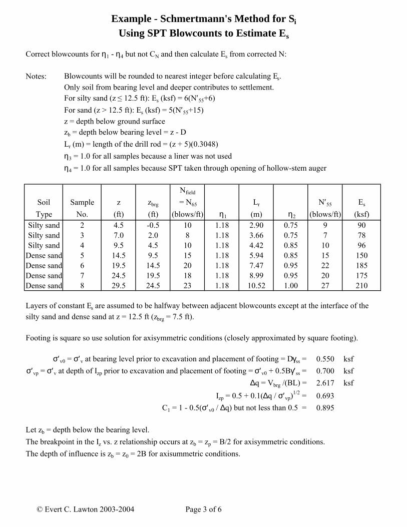
Correct blowcounts for η1 - η4 but not CN and then calculate Es from corrected N:

Notes: Blowcounts will be rounded to nearest integer before calculating Es.Only soil from bearing level and deeper contributes to settlement.For silty sand (z ≤ 12.5 ft): Es (ksf) = 6(N′55+6)For sand (z > 12.5 ft): Es (ksf) = 5(N′55+15)z = depth below ground surfacezb = depth below bearing level = z - DLr (m) = length of the drill rod = (z + 5)(0.3048)η3 = 1.0 for all samples because a liner was not usedη4 = 1.0 for all samples because SPT taken through opening of hollow-stem auger

Nfield

Soil Sample z zbrg = N65 Lr N′55 Es

Type No. (ft) (ft) (blows/ft) η1 (m) η2 (blows/ft) (ksf)Silty sand 2 4.5 -0.5 10 1.18 2.90 0.75 9 90Silty sand 3 7.0 2.0 8 1.18 3.66 0.75 7 78Silty sand 4 9.5 4.5 10 1.18 4.42 0.85 10 96

Dense sand 5 14.5 9.5 15 1.18 5.94 0.85 15 150Dense sand 6 19.5 14.5 20 1.18 7.47 0.95 22 185Dense sand 7 24.5 19.5 18 1.18 8.99 0.95 20 175Dense sand 8 29.5 24.5 23 1.18 10.52 1.00 27 210

Footing is square so use solution for axisymmetric conditions (closely approximated by square footing).

σ′v0 = σ′v at bearing level prior to excavation and placement of footing = Dγss = 0.550 ksfσ′vp = σ′v at depth of Izp prior to excavation and placement of footing = σ′v0 + 0.5Bγ′ss = 0.700 ksf

∆q = Vbrg /(BL) = 2.617 ksfIzp = 0.5 + 0.1(∆q / σ′vp)

1/2 = 0.693C1 = 1 - 0.5(σ′v0 / ∆q) but not less than 0.5 = 0.895

Let zb = depth below the bearing level. The breakpoint in the Iz vs. z relationship occurs at zb = zp = B/2 for axisymmetric conditions.The depth of influence is zb = z0 = 2B for axisummetric conditions.

Layers of constant Es are assumed to be halfway between adjacent blowcounts except at the interface of the silty sand and dense sand at z = 12.5 ft (zbrg = 7.5 ft).




zp = 2.5 ftz0 = 10 ft

Write equations for lines of Iz vs. zb. There are two lines - one from bearing level to zp, and one from zp to z0.

From the bearing level to zp: Iz = 0.1 + (Izp - 0.1)/(B/2)*zb

Iz = 0.1 + 0.2373 zb

From zp to z0: Iz = Izp - Izp/(1.5B)*(zb - 0.5B) = 4/3*Izp - Izp/(1.5B)*zb

Iz = 0.924 - 0.0924 zb

Layer Soil zb(top) zb(bot) ∆z zb Avg. Es Iz*∆z/Es

i Type (ft) (ft) (ft) (ft) Iz (ksf) (ft/ksf)1 Silty sand 0.00 0.75 0.75 0.375 0.189 90 0.001582a Silty sand 0.75 2.50 1.75 1.625 0.486 78 0.010902b Silty sand 2.50 3.25 0.75 2.875 0.659 78 0.006333 Silty sand 3.25 7.50 4.25 5.375 0.428 96 0.018934 Dense sand 7.50 10.00 2.50 8.75 0.116 150 0.00193

Σ∆z = 2B = 10 ΣIz*∆z/Es = 0.03966

Si = C1*∆q* ΣIz*∆z/Es = 0.0929 ft = 1.11 in.

Layer Soil zb(top) zb(bot) ∆z zb Avg. Es Iz*∆z/Es

i Type (ft) (ft) (ft) (ft) Iz (ksf) (ft/ksf)1 Silty sand 0.00 0.75 0.75 0.375 0.189 90 0.001582a Silty sand 0.75 2.50 1.75 1.625 0.486 78 0.010902b Silty sand 2.50 3.25 0.75 2.875 0.659 78 0.006333 Silty sand 3.25 7.00 3.75 5.125 0.451 96 0.017604 Dense sand 7.00 10.00 3.00 8.5 0.139 150 0.00277

Σ∆z = 2B = 10 ΣIz*∆z/Es = 0.03918

Si = C1*∆q* ΣIz*∆z/Es = 0.0918 ft = 1.10 in.

SUMMARY OF ANSWERS: From Schertmann's method, Si = 1.1 in.

Could also define layers strictly halfway between adjacent blowcounts, which would modify layers3 and 4 only.








7302 May, 1970 SM 3

Journal of the

SOIL MECHANICS AND FOUNDATIONS DIVISION

Proceedings of the American Society of Civil Engineers

STATIC CONE TO COMPUTE STATIC SETTLEMENT OVER SAND

By John H. Schmertmann,’ M. ASCE

INTRODUCTION

Settlement, rather than bearing capacity (stability) criteria, usually exert the design control when the least width of a foundation over sand exceeds 3 ft to 4 ft. Engineers use various procedures for calculating or estimating settlement over sand. Computations based on the results of laboratory work, such as oedemeter and stress-path triaxial testing, involve trained personnel, considerable time and expense, and first require undisturbed sampling. Inter- preting the results from such testing often raises the serious question of the effect of sampling and handling disturbances. For example: Does the natural sand have significant cement bonding even though the lab samples appear cohesionless? When dealing with sands many engineers prefer therefore to do their testing in-situ.

Settlement studies based on field model testing, such as the plate bearing load test, often require too much time and money. This type of testing also suffers from the serious handicap of long-existing and still significant un- certainties as to how to extrapolate to prototype foundation sizes and non- homogeneous soil conditions. A new type of test for field compressibility, involving a bore-hole expanding device or pressuremeter, is now also used in practice. The accuracy of a settlement prediction using such devices and semi-empirical correlations is not yet, to the writer’s knowledge, documented in the English literature and may not yet be established. Whatever its prediction accuracy, such special testing and analysis should prove more expensive than settlement estimates based on the results of field penetrometer tests.

Presently, engineers commonly use settlement estimate procedures based on two very different types of field penetrometer tests. U.S. engineers have used the Standard Penetration Test for 29 yr. The hammer blow-count, or N-value, has been empirically correlated to plate test and prototype footing

Note.-Discussion open until October 1, 1970. To extend the closing date one month, a written request must be filed with the Executive Secretary, ASCE. This paper is part of the copyrighted Journal of the Soil Mechanics and Foundations Division, Proceedings of the American Society of Civil Engineers, Vol. 96, No. SM3, May, 1970. Manuscript was submitted for review for possible publication on January 22, 1969.

‘Prof. of Civil Engrg., Univ. of Florida, Gainesville, Fla.

1011

Roger A. Failmezger

Reference Source: Journal of the Soil Mechanics and Foundations Division, Vol. 96, No. SM3, May 1970, ASCE, New York, New York

1012 May, 1970 SM3

settlement performance. Because of the completely empirical nature of this method the engineer sometimes finds it not very informative or satisfying to use. Some engineers believe that it often results in excessively conservative (too high) settlement predictions. Another method, based on the Static Cone Penetration Test, has a European history of over 30 yr. In this method the quasistatic bearing capacity of a steel cone provides an indicator of soil compressibility. Settlement predictions have proven conservative by a factor averaging about 2.0.

The field penetrometer methods have the great advantage of practicality, with results obtained in-situ, quickly, and inexpensively. These advantages permit testing in volume, and thereby permit a better evaluation of any important consequences resulting from the nonhomogeneity of most sand foundations.

Perhaps the empirical nature of the present penetrometer methods represents their greatest disadvantage. The engineer does not find it easy to trace the logic and data to support these methods. Herein he will find a new approach, based on static cone penetrometer tests, which has an easily understood theoretical and experimental basis. Compared to thebest procedure now in use, this new method has a more correct theoretical basis, results in simpler computations, and test case comparisons suggest it will often result in more accuracy without sacrificing conservatism.

CENTERLINE DISTRIBUTION OF VERTICAL STRAIN

Engineers have often assumed that the distribution of vertical strain under the center of a footing over uniform sand is qualitatively similar to the distribution of the increase in vertical stress. If true, the greatest strain would occur immediately under the footing, the position of greatest stress increase. Recent knowledge all but proves that this is incorrect.

Elasticity and Model Studies.-Start with the theory of linear elasticity by considering a uniform circular loading, of radius = r and intensity = p, on the surface of a homogeneous, isotropic, elastic half space. The vertical strain at any depth z = l z, under thecenter of the loading, follows Eq. 1 from Ahlvin & Ulery (1):

EZ = 2 (1 + v) [(l - 2v)A f F] . . . . . . . . . . . . . . . . . . . . . . . (1)

in which A and F = dimensionless factors that depend only on the geometric location of the point considered; and E and v = the elastic constants.

Because p and E remain constant, the vertical strain depends on a vertical strain influence factor, 2,. Thus

Z, = (1 + v) [(l - 2v)A + F] . . . . . . . . . . . . . . . . . . . . . . . . . (2)

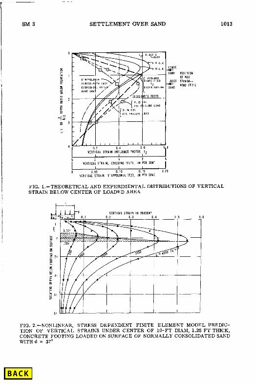
Fig. 1 shows the distribution of this influence factor, and therefore strain multiplied by the constant E/p, with a dimensionless representation of depth for Poisson’s ratios of 0.4 and 0.5. The area between the I, = 0 axis and these curves represents settlement. Note that maximum vertical strain does not occur immediately under the loading, where the increase in vertical stress is its maximum, l.Op, but rather at a depth of (Z/Y) = 0.6 to 0.7, where the Boussinesq increase in vertical stress is only about O.Sp.

SM 3 SETTLEMENT OVER SAND

WITH 4 = 37’

I I I I - 1 Q 2 4 6 a

VERTlCAL STRAIN, EGGLSTilQ TESTS. IN PER CENT I I I

Q 0.05 0.10 0.15 0.20 YERT,CLL STMIW. Q’LPPQLQtl,)I TEST, It4 PER CENI

FIG. l.-THEORETICAL AND EXPERIMENTAL DISTRIBUTIONS OF VERTICAL STRAIN BELOW CENTER OF LOADED AREA

FIG. 2.-NONLINEAR, STRESS DEPENDENT FINITE ELEMENT MODEL PREDIC- TION OF VERTICAL STRAINS UNDER CENTER OF lo-FT DIAM, 1.25 FT THICK, CONCRETE FOOTING LOADED ON SURFACE OF NORMALLY CONSOLIDATED SAND

1013

POSITION OF MLX. SINLIN-- BONO TESTS

.6

1014 May, 1970 SM 3

Evidence similar to that previously given would result from considering uniformly loaded rectangular areas of least width = B. The writer obtained the following from the elastic settlement solutions tabulated by Harr (15): the maximum vertical strain under both the center and corner of a square occurs at a depth z/B/2 = 0.8 and 0.6 for Poisson’s ratio = 0.5 and 0.4, respectively; the corresponding relative depths to maximum strain under a rectangle with L/B = 5 are 1.1 and 0.9.

Model studies using sand all show that the depth to maximum vertical strain increases compared to that indicated by elastic theory. Fig. 1 includes two representative vertical strain distributions from Eggestad’s (10) tests on homogeneous sand under a rigid, circular footing of radius = Y. He reports a depth to maximum verticalstrain of about (Z/Y) = 1.5 for bothloose and dense sand. Eggestadalso reported the results of a similar model study by Bond (5) with depth to maximum vertical strain at (Z/Y) = 0.8 for dense sand and 1.4 for loose sand. Holden (16)using a uniformly loaded circular area on the surface of a medium sand with a relative density of 670/o, reports maximum vertical strain at z/Y = 1.1.

Vertical strain distributions have also been reported from the results of stress path tests on triaxial specimens of reassembled sand. Fig. 1 includes one from Ref. 6, from test results on a dense, overconsolidated sand.

Finite Element Computer Simulation .-A comprehensive, computer modeling technique has also been employed to study the axial-symmetric strain distributionunder a circular, concrete footing resting on the surface of homogeneous sand. The finite element technique permits modeling the soil realis- tically, as a materialwith gravity stresses, nonlinear stress-strain behavior, and with stress-strain behavior dependent on effective stress. Fig. 2 presents some computer predicted, centerline strain distributions for one specific case: a lo-ft diam concrete footing, 1.25 ft thick, resting on the surface of a homogeneous, cohesionless soil with Q = 37”, and with unit weight = 100 lb per cu ft. (For the cases studied the vertical strain distributions were almost the same from the center line to between 0.5~ to 0.75r.) This model soil aIso has K, = 0.50 and Poisson’s ratio = 0.48, thus approximating a normally consolidated state.

The computer-predicted settlements of this footing increase linearly to about 0.8 in, when p = 4,000 psf-a reasonable value for a real sand with o = 37”. In view of the strain information in Fig. 1, the strain distributions in Fig. 2 also appear reasonable. (This is a preliminary study, done in June, 1969, by J. M. Duncan at the University of California, Berkeley, for Nilmar Janbu and the writer.) The depth to greatest vertical strain gradually increases asp increases,from about 0.72~ at 500 psf to 1.20~ at 4,000 psf. The same analysis, but with a lOO-ft diam footing, results in a similar strain distribution, but with the depth to maximum strain remaining at about 0.72~ while p increases from 1,000 psf to 4,000 psf. Results are also similar witha l.O-ft diam footing, but depth to maximum strain increases from about 0.75r to l.l9r, whilep increases from 50 psf to 500 psf. It seems clear that the depth to maximum, centerline, vertical strain increases at the ratio of structural/ gravity stresses increases. However, the increase is only over the 0.7~ to 1.2~ range. Both this range ofdepths to maximum strain, and the shape of the strain distribution curves, tend to confirm the other types of similar data presented in Fig. 1.

This computer study also showed that over the range of diameters investi-

SM 3 SETTLEMENT OVER SAND 1015

gated, 1 ft to 100 ft, and over the range of footing pressure investigated, 50 psf to 4,000 psf, approximately 90% of the settlement occurred within a depth = 4r below the footing. From a practical viewpoint, it seems reasonable to reduce exploration and computation by ignoring the static settlement of sand below 4~.

Single, Approximate Distribution.-From the theoretical, model study, and experimental and computer-simulation results, it seems abundantly clear that the vertical strain under shallow foundations over homogeneous, free draining soils proceeds from a low value immediately under a footing to a maximum at a significant depth below the footing and thereafter gradually diminishes with depth. This is considerably different than one would expect when assuming a vertical strain distribution similar to the distribution of increase in vertical stress. Such an assumption is likely to be incorrect. The reason it is incorrect is that vertical strains in a stress dependent, dilatent material such as sand depend not only on the level of existing and added vertical normal stress, but also on the existing and added shear stresses and their respective ratio to failure shear stresses. The importance of shear in settlement has been noted repeatedly, by DeBeer (8), Brinch Hansen (131, Janbu (17), Lambe (21), and Vargas (38).

Considering the evidence in Figs. 1 and 2, for practical work it appears justified to use an approximate distribution for the vertical strain factor, I,, under a shallow footing rather than to work indirectly through an approximate distribution of vertical stress. Why use an unnecessary and uncertain intermediate parameter? Possibly the most accurate estimate of a distribution for the strain factor for a particular problem would involve a complex consideration of the vertical distribution of changes in deviatoric and spherical stress. Each problem would then involve a special distribution. However, as shown subsequently by test cases, a single, simple distribution seems accurate enough for many practical settlement problems. The writer suggests the triangular distribution shown by the heavy, dashed line in Figs. 1 and 6 for the approximate distribution of a strain influence factor, Zz, for use in design computations for static settlement of isolated, rigid, shallow foundations. The writer uses this I, triangle, referred to as the 2B-0.6 distribution, throughout the remainder of this paper.

The approximate distribution defines a vertical strain factor, and not vertical strain itself. Eqs. 1 and 2 show that this factor requires multiplication byp/E to convert it to strain.

This approximate distribution for the strain factor, which equals the shape of the actual strain distribution for a sand with constant modulus, applies only under the center portion of a rigid foundation. However, with knowledge of the vertical strain distribution under any point of the foundation the engineer can solve for the settlement of a concentrically loaded, rigid foundation. This is the case assumed herein. Consideration of other cases requires extension of this work.

CORRECTIONS TO ASSUMED APPROXIMATE STRAIN DISTRIBUTION

Foundation Embedment.-Embedding a foundation can greatly reduce its settlement under a given load. For example, Peck et al. (29) suggests a reduction factor of 0.50 when D/B changes from 0 to 4. D = the depth of foun-

1016 May, 1970 SM 3

dation embedment and B = the least width of a rectangular foundation. Teng (34) suggests a reductionfactorof 0.50 when D/B changesfrom 0 to 1. Meyer- hof (25) suggests 0.75 for the same embedment. Yet, no major change in the 2B-0.6 I, distribution is required to correct for embedment when using cone data.

Cone bearing values in sand soils usually start from low values at the surface and increase with depth. Thus, even with homogeneous soil, a surface foundation would have an average cone value over the O-2B interval that can be considerably less than the average value over B-3B, which becomes the 2B interval when D = B. For example, if qc increased proportional to the square root of z/B, from zero at the surface, then settlement when D/B = 1 computes about 0.60 the settlement when D/B = 0, and about 0.35 of this settlement when D/B = 4 (using the new method described later).

Another, usually relatively minor, correction for embedment results from the use of elastic theory. According to solutions from the linear theory of elasticity, once the depth, D, of a buried square footing exceeds about five times its least width, B, then elastic settlement reduces to one-half surface values (15). The assumed elastic, weightless material above the level of loading permits tension to relieve load and strain under that level. Sands, contrary to this, cannot sustain loads in tension. However, an arching-induced reduction in compressive stresses can replace elastic tension, with the compressive stresses due to the overburden weight of the sand.

To take some account of the strain relief due to embedment, and yet retain simplicity for design purposes, the writer proposes to retain the 2B-0.6 shape of the strain influence factor, I,, but to adjust its maximum value to some- thing less than 0.6. To conform to the arching-compression relief concept this adjustment should not depend solely on the D/B ratio. Instead use the ratio of the overburden pressure at the foundation level, = PO, to the net foundation pressure increase, = (# - p,) = Afi, or (&/AD). The following equation defines a simple, linear correction factor, C, :

c, = 1 - 0.5 G ( >

. . . . . . . . . . . . . . . . . . . . . . . . . . . . . . . . (3)

However, in accord with elasticity, C, should equal or exceed 0.5. Creep.-In the past it has not been common to consider the time rate of

development of settlement in sand. Contrary to this, many, but not all, of the published settlement records show settlement continuing with time in a manner suggesting a creep type phenomenon.

Brinch Hansen (13) noted the importance of this creep and included a mathe- matical estimate of its contribution in his sand settlement analysis procedure. Nonveiler (28) also noted its importance and suggested this linear decay correction on a semilog plot:

pt = p. 1 + p log + C ( )I . . . . . . . . . . . . . . . . . . . . . . . . . . . . 0 in which p. = the settlement at some reference time to; pt = the settlement at time t and /3 = a constant which was about 0.2 to 0.3 in the problem investigated. The apparent creep is not completely understood and most likely arises from a variety of causes. But, the effect is similar to secondary compression in clay. Because of the simplicity of Eq. 4, the writer has adopted it


as a correction factor, Ca, in this new settlement estimate procedure. Tenta- tively, @ = 0.2 and the reference time, t, = 0.1 yr. The principal justification for this reference time is that it is convenient and appears togive reasonable predictions in the test cases noted subsequently. Then C, becomes:

c, = 1 + 0.2 log ( ) Lx o.1 , . . . . . . . . . . . . . . . . . . . . . . . . . . . .

Shape of Loaded Area.- The various shape correction factors used when applying the theory of elasticity to the settlement of uniformly loaded surface areas suggests that the distribution of the assumed strain influence factor, I,, also needs modification according to the shape of the loaded area. However, a correction does not appear necessary at this time.

Consider a rectangular foundation of constant, least width = B and with constant bearing pressure = p. As its length L, and L/B, increases the total load on the foundation increases and one might therefore expect a greater settlement although both B and p remain constant. However conditions also become progressively more plane strain. The full transition from axially symmetric to plane strain involves some increase in the angle of internal friction. This increased strength results in reduced compressibility, which tends to counteract the effect of a larger loaded area and a larger load. Neither behavior is well enough understood over a range of L/B ratios to permit preparing quantitative shape factor corrections. The writer assumes herein that these compensating effects cancel each other. It may be significant to note that no such correction is used with SPT empirical methods. The subsequent test cases, involving a considerable range of L/B ratios, also do not suggest an obvious need for such correction.

Adjacent Loads.-The design engineer must also deal with the practical problem of how to compute the settlement interaction between adjacent foundation loadings. This complicated problem involves a material (sand) with a nonlinear, stress dependent, stress-strain behavior. Not only do strain and settlement depend on the position and magnitude of adjacent loads, but also on their sequence of application. A later application of a smaller, adjacent load should settle less, possibly much less, than had that load been applied without the lateral prestressing effects of the first load.

In stress oriented settlement computation procedures the adjacent load problem is ordinarily handled by assuming linear superposition of elastic stresses. The analogous in a strain oriented procedure would be to superpose strains, or strain influence factors. However, any simple, linear form of superposition possibly invites serious error because of the nonlinear importance of stress magnitude and loading sequence. More research is needed to formulate design rules for this problem. Model studies, in the laboratory or by computer simulation, or both, look most promising.

The present state of knowledge requires the engineer to use conservative judgement. Obviously if two foundations are far enough apart any interaction will be negligible. The writer would consider this the case if 45” lines from the edges intersect at a depth greater than 2B,, when a second loading of width B, is placed next to an existing foundation of greater width B,. For a 45” intersection depth also greater than B1, assume them independent re- gardless of load sequence. If adjacent foundations are close enough to interact without question, say thedistance between them is less than B of the smallest and they are loaded simultaneously, then the writer would treat them as a

1018 May, 1970 SM 3

single foundation with some appropriate, equivalent width. Intermediate situ- ations should fall within these boundaries.

CORRELATION BETWEEN STATIC CONE BEARING CAPACITY AND E, VALUES USED IN SETTLEMENT COMPUTATIONS

Continuing the previous notations, the calculation of settlement requires an integration of strains. Thus

P = _r eZdz m AP fB dz FJ C,C,AP “c” 0 0 0

The last form of Eq. 6 permits approximate integration and a way of accounting for soil layering. The key soil-property variable that still remains to be determined is the equivalent Young’s modulus for thevertical static compression of sand, Es, and its variation with depth under a particular foundation.

Screw-Plate Tests.-A direct means of determining vertical E, in sands would be to test load a plate in-situ, measure its settlement, and use Eq. 6 to backfigure its modulus. Any attempt to test at depths other than near the surface requires an excavation with its attendant load-removal stress and strain disturbances. Many sites would also require dewatering, with still further stress disturbances. To avoid such difficulties the writer used a form of plate bearing load test used in Norway (19), known as the screw-plate test. The writer’s screw-plateconsisted of an auger with a pitch equal to l/5 its diameter, and a horizontally projected area of 1.00 sq ft over a single, 360” auger flight. This special auger was screwed into the ground, taking care to assure that the vertical rods remain plumb. The buried plate was loaded by using a hydraulic jack at the surface, reacting against anchored beams. Rod friction to the screw-plate seemed negligible. Elastic compression was subtracted and care was used to assure the column of rods to the plate did not buckle significantly. Sands at depths from 3 ft to 26 ft (1 m to 8 m) were tested in this way.

Fig. 3 shows photographs of the screw-plate and the load test set-up. The load was applied to the top of the column of rods, using increments in the conventional manner. The usual results consisted of a conventional appearing load-settlement curve with tangent moduli decreasing slightly with increasing pressure.

Correlation with Static Cone Bearing.-Although the screw-plate type of load test to determine sand compressibility is faster and less expensive than burying a rigid plate, it is nevertheless still too time consuming for routine investigations. For this reason data were accumulated in an attempt to see if static cone bearing capacity would correlate with screw-plate bearing compressibility. Fig. 4 presents the results of this correlation on a log-log plot. This investigation used the mechanical Dutch friction cone (32), advanced at the common rate of 2 cm per sec. Sand compressibility, in inches per ton per square foot (tsf), was taken as the secant slope over the 1 tsf-3 tsf increment of plate loading. This interval was chosen for convenience because the seat- ing load was 0.5 tsf, almost all tests were carried to a minimum of 3 tsf, and real footing pressures commonly fall within this interval.

Note that a different symbol denotes each of 10 test sites. Four of these are in Gainesville, Florida. The remaining six are within a radius of about

SM3 SETTLEMENT OVER SAND 1019

FIG. 3.-UNIVERSITY OF FLORIDA SCREW-PLATE LOAD TEST: (a) 1.0 SQ FT SCREW-PLATE; (h) LOAD TEST SET-UP

II

r II

1.0

FIG. (.-EXPERIMENTAL CORRELATION BETWEEN DUTCH CONE BEARING CA- PACITY AND COMPRESSIBILITY, UNDER IN-SITU SCREW-PLATE LOAD TEST, OF SOME FINE SANDS IN FLORIDA

1020 May, 1970 SM 3

150 miles from Gainesville. The sands tested were above the water table, and include silty fine sand to uniform medium sand. However, most tests involved only fine sand with a uniformity coefficient of 2 to 2.5.

Fig. 4 includes 29 screw-plate tests from two research sites on the campus of the University of Florida. To condense the results from these 29, Fig. 4 shows only the average values for each group of tests at the same depth at the same site. Dashed lines indicate the spread of the data from one site. These special research tests involved only two plate depths, 2.8 ft and 6.1 ft. Nine tests were also made on 1.0 sq ft rigid, circular plates at these same plate depths at one of these sites. Again, average values and spread are indicated. The adjacent number indicates the number of individual tests in the average. The eight remaining sites account for 24 screw,-plate tests at depths ranging from 3 ft to 26 ft, averaging 9.3 ft. At one of these sites data were also available from three 1-ft square rigid plate tests by Law Engineering Testing Co. Thus, the total number of individual plate tests included in Fig. 4 consists of 53 screw-plate and 12 rigid plate tests.

It appears from Fig. 4 that about 90% of these data fall within the factor- of-2 band shown. It is not surprising that a good correlation exists between compressibility and cone bearing in sands because in some ways the penetration of the cone is similar to the expansion of a spherical or cylindrical cav- ity, or both (2). Alternatively, if the cone is thought of as measuring bearing capacity and hence shear strength, then one can also argue, as the writer has already done, that the compressibility of sand is greatly dependent on its shear strength.

To convert screw-plate compressibility into E, values required for Eq. 6 only required backfiguring that E, value needed to satisfy Eq. 6 and each measured settlement. This resulted in the correlation in Fig. 5. Because the grouping of the individual points proved similar to that in Fig. 4, only the factor-of-two- band is shown (dashed lines). With this band as a guide the writer then chose a single correlation line for design in ordinary sands. Thus

E, = 2 qc . . . . . . . . . . . . . . . . . . . . . . . . . . . . . . . . . . . . . . (7)

This line was chosen because it falls within the screw-plate band, because it results in generally acceptable predictions for settlement in the subsequent test cases and also because of its simplicity. Eq. 7 permits the use of inex- pensive cone bearing data to estimate static sand compressibility, as represented by E,. Then compute settlement from Eq. 6.

Webb (40) recently reported the results of an independent correlation study in South Africa between the insitu screw-plate compressibility of fine to medium sands below the water table and cone bearing. His data include seven tests using a 6-in. diam plate (0.20 sq ft), eight tests with a g-in. plate (0.44 sq ft) and one test with a 15-in. plate (1.23 sq ft). Cone bearing rangedbetween about 10 tsf and 100 tsf. He offers the following correlation equation for con- verting qc to his E’:

E’ (tsf) = 2.5 (qc + 30 tsf) . . . . . . . . . . . . . . . . , . . . . . . . . . (8)

Comparisonof the elastic settlement formula in his paper and Eq. 6 herein shows that E, = C,C, 0.6 E’. This assumes a constant E, for a 2B depth below the screw-plate, permitting C I, AZ = area under 2B-0.6 Zz distribution = 0.6OB. The average product C,C, used by the writer when convert- ing his screw-plate data was about 0.88. Thus, E, = 0.53 E’. Webb’s equation


then converts to Es FJ 1.32 (qc + 30). Further comparison with Eq. 7 now shows the same prediction for E, when qc a 60 tsf, and a difference of 20% or less when qc lies between 35 tsf and 170 tsf. Reference to Tables 1 and 2 shows that this range includes most natural sands. Such agreement supports the validity of using cone bearing data to estimate the insitu compressibility of sand under a screw-plate.

MethodofAccounting forSoil Layering, Including a Rigid Boundary Layer.- The simple I, distribution developed herein from elastic theory and model experiments assumed or used a homogeneous foundation material. But, sand deposits vary in strength andcompressibility with depth. It is further assumed that the I, distribution remains the same irrespective of the nature of any

RECOMMENOEO FOR

FACTOR-OF-P BAND

WITHIN WHICH FALLS

MOST OF SCREW-PLATE DATA

(SEE FIG. 4)

1 I 1 I

20 40 100 200 400

GC = DUTCH CONE BEARING CAPACITY

in kg/cm2 (P tons/ft*)

FIG. 5.-CORRELATION BETWEEN q, AND E, RECOMMENDED FOR USE IN ORDINARY DESIGN

such layering and that the effects of such layering are approximately, but adequately, accounted for by varying the E, value in Eq. 6 in accord with Eq. 7.

It is possible that the above method of accounting for layering represents an oversimplification and will result in serious error under special circum- stances not now appreciated. More research would be useful to define the limitations of this method and to improve it. Model studies, especially computer simulation using the nonlinear, stress dependent finite element technique, appear to have great promise for investigating such problems. This approach to layering also includes the treatment of a rigid boundary layer en- countered within the interval 0 to 2B. The 2B-0.6 I, distribution remains the same but the soils below this boundary, to the depth 2B, are assumed to have a very high modulus. Vertical strains below such a boundary then become negligible and can be taken equal to zero.

1022 May, 1970 SM 3

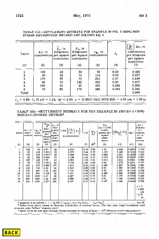
TABLE I(U).--SETTLEMENT ESTIMATE FOR EXAMPLE IN FIG. 6 USING NEW STRAIN-DISTRIBUTION METHOD AND SOLVING EQ. 6

-

( P I

-

Qc, in tilogramc ,er squar, :entimete:

‘L .ES >

AZ, in

centimeters ler kilogram per square centimeter

(7)

E,, in kilograms ,er square :entimeter

(4)

z,, in centimeters Layer

AZ, in centimeter

(‘3) (1) (5)

1 2 3 4 5 6

Total

25 35 35 70 30 05

50 50 0.23 70 115 0.53 70 215 0.47

140 325 0.30 60 400 0.185

170 485 0.055

0.462 0.227 1.140 0.107 0.308 0.022 2.266

C, = 0.89; C, (5 yr) = 1.34; Ap = 1.50; p = (0.89)(1.34)(1.50)(2.266) = 4.05 cm = 1.6oin.

TABLE l(b).-SETTLEMENT ESTIMATE FOR THE EXAMPLE IN FIGURE 6 USING BUISMAN-DEBEER METHODa

Layel

(1)

iz, in xnti- neter,

(2) (3)

= Gt

ik kilo-

:ram

Per KJ”U centi mete

(4)

50 0.31 115 0.436 215 0.535 325 0.645 400 0.72 415 0.195 575 0.995 700 1.02 800 1.12 925 1.245

1050 1.37 1200 1.52 1350 1.67C

-

-

),

” (

4 A* = 1.50

in kilograms per

SCJ”IlR centimeter

(9) (6) (7) wb

2.212 0.19 0.90 0.573 0.44 0.75 3.966 0.63 0.59 0.706 1.25 0.47 3.664 1.54 0.41 0.716 1.63 0.36 1.213 2.21 0.31 2.610 2.69 0.26 1.719 3.06 0.22 1.167 3.56 0.19 3.161 4.04 0.16 3.886 4.62 0.14 2.137 5.19 0.12

1 2 3 4 5 6 7 8 9

10 11 12 13

100 30

110 50

100 50

150 100 100 150 100 200 100

-

25 35 35 10 30 65

170 60

100 40 66

120 120

1.35 1.125 0.665 0.105 0.615 0.54 0.465 0.39 0.33 0.265 0.24 0.21 0.16C

2.093 0.3206 0.227 1.654 0.2681 0.986 1.679 0.2251 0.161 1.520 0.1616 0.221 1.382 0.1405 0.367 1.295 0.1123 0.193 1.229 0.0696 0.642 1.175 1.136 1.108

p=L?

= 6.660

I I = 2.;om in.

aEquation to be solved: P = C {1.535 [( o:</qc) AZ] log [(AU, + o;,)/o:j]} . . . Eq. (9) bTaken from charts based on Buisman distribution of vertical stress. For this case (rigid foundation) used

stresses under DeBeer ‘singular point’. C Layer 13 is the last layer because stress increase at bottom of layer = 10% effective overburden pressure.


Justification for the previous approach is primarily pragmatic. The computational procedure retains its simplicity despite layering. This method appears successful in the test cases noted subsequently, including the case with a rigid boundary at 0.23B. Also, a series of model tests by the writer, using a circular, rigid, plate of 2.3 in. diam, on the surface of a dry sand with a relative density of about 25%, showed the effect of a rigid boundary on settlement to be very similar to that obtained from the 2B-0.6 I, distribution and the simple cut-off procedure previously suggested.

The simple conversion from cone bearing to modulus suggested herein could require modification for such effects as the magnitude of foundation pressure increase, different ground water conditions and different states of overconsolidation. This topic falls beyond the scope of the present paper. No such corrections are suggested herein. The subsequent test case comparison results suggest that the simplest approach, ignoring them, often produces acceptable prediction accuracy.

SETTLEMENT ESTIMATE CALCULATION

The following information must be gathered before a settlement estimate can be computed by the method suggested herein:

1. A static cone bearing capacity ( qc) profile over the depth interval from the proposed foundation level to a depth below this of 2B, or to a boundary layer that can be assumed incompressible, whichever occurs first. Because the correlation with E, is empirical and is based on qc values obtained primarily from Dutch static cone equipment, it is desirable that the needed qc profile be obtained with similar equipment. The Dutch cone has a 60’ hardened steel point, a projected end area of 10 sq cm, and is advanced during a mea- surement at a rate of 2 cm per sec. The rods above the points are screened from soil friction by an outer, casing rod system. Other static cone systems may be used provided they can be correlated with the Dutch cone results or provided independent calibrations with E, can be established for each system.

2. The least width of the foundation = B, its depth of embedment = D,

and the proposed average foundation contact pressure = p. The same data is needed for adjacent foundations close enough to interact with the one for which settlement is being estimated.

3. The approximate unit weights of surcharge soils, and the position of the water table if within D. These data are needed for the estimate of p,,, which is needed for the C, correction factor.

With this information gathered, proceed as in the example illustrated by Fig. 6 and Table l(a). This example is an actual pier foundation and is the first test case comparison in the next section herein.

4. Divide the qc profile into a convenient number of layers, each with constant vc, over the depth interval 0 to 2 B below the foundation.

5. Prepare a table with headings similar to Table l(u) herein. Fill in columns 1, 2, and 3 with the layering assigned in step 4.

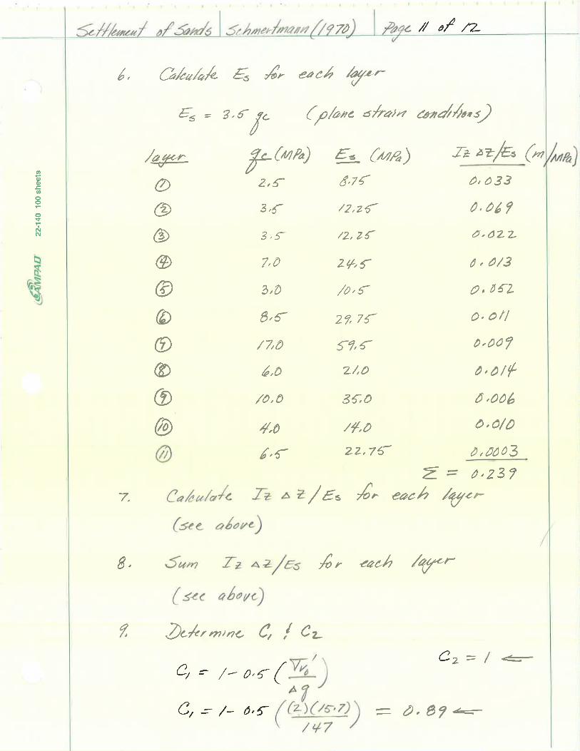
6. Multiply the values of qc in column 3 by the factor 2.0 to obtain the suggested design in values of E,. Place these in column 4.

7. Draw the assumed 2B-0.6 triangular distribution for the strain influ-

1024 May, 19’70 SM 3 SM 3 SETTLEMENT OVER SAND 1025

OF TEST CASES TABLE 2. -IBTING

- .4

Soil

0”. i

I

(7)

pproxi- mate verage

-28 9c, n kilo- :rams

Per square centimeter

(8)

Foundation at ground-water table

40

Silty to fine sand 1 20

Cut in sand, some clay lS.yel-S

2 120

1

Coarse silt, fine sand, ground- water table at surface

Fine sand, l/3 calcite (shells)

20

70 60

90

Natural fine sand, above ground-water table

I

Compacted moist sand embankment

Compacted moist sand embankment, but water at base of pier

135 LOO LOO

180 150

70 55

45 45 35

Uniform, very fine sand above ground-water table

Vibrofloted sand below water table

Alluvial sand below ground water table

18 22 20 23 21 32

80 70

125 to 0.5!

40

.Y Variety of sands, smne cla and silt

I- Hydraulic fill below grounc water table

Fine sand, slightly organic below ground-water table

Gravel with flints, sane fine sand

Overconsolidated dune sari d

115 100

30

70

130

120

1 -

-

r St F

- -

Number Reference B, in feet

-

1 D/B

(1) (2)

structure

(3)

-

5/B

(5) (6)

1 )eBeer (9) 3elgian bridge pier

(4)

8.5 8.8 0.78

2 )eBeer (9) 3elgian bridge pier 9.8 4.2 1.0

3 )eBeer (7) 3elgian bridge pier 8.2 2.5 1.2

4

5

rleI3eer (7)

3jerrum (3,201

Belgian bridge pier 19.7 2.7 0.58

rest fill 62 1.0 0

6 \Tonveiler (28) 3rain silo 81 2.2 0.1

I Muhs (27) Test: V

VI XI

Model concrete pier load tests

VI&M x, XII

xv, XVII XVI, XVIII

XXKVII KXXVIII

XKKIX

3.3 1.1 1.7

3.3 1.1 3.3 1.64

3.3 3.3 1.64

1.0 3.9 3.9

1.0 3.9 1.0 4.0

1.0 1.0 4.0

0 0 0

0.5 1.0 0.5 1.0

0.5 0.5 1.0

8 Law load test in Florida

NO 5 e 7

a 9

1c

9a Tschebotarioff (37) 9b Tschebotarioff (37)

10 Grimes and Cantlay (12)

Steel plate Steel plate Concrete plate Concrete plate Concrete plate concrete plate

Liquid storage building Test plate

20 St Office Building (center Of 3)

2.0 1.0 0.55 2.0 1.0 1.5 3.0 1.0 0.3 3.0 1.0 1.0 4.0 1.0 0.17 4.0 1.0 0.75

90 1.1 0.1 2.0 1.0 0

42.7 2.1 0.16

11 Webb (40) Concrete test plate 20 1.0 0.03

12 Bogdanovic (4) B-story apartment 79 3.6 0

13 Brinch Hansen (13) Steel tank 184 1.0 0

14

15

Kumennje (19) Janb” (18)

Meigh and Nixon (23)

Oil Tank 96 1.0 0

Factory concrete footing 4.7 1.0 0.85

16 D’Appolonia (6) over 300 steel factory footings

12.5 1.6 0.64

+ - - -

resses, in tons 1er square foot

PO

(9)

3.33

AP

(10)

Notes

(11)

0.33

0.54

1.21 1.70

1.27 1.86

2.43

No live load Full live load

No live load Full live load

Probably full live load

0.64

0

1.78

0.18

Probably full live load

Nearest qc

average 2 nearest

0.56 2.07 Rock below D = I3

0 2.05 0 2.05 0 3.07

0.10 5.16 0.10 5.16 0.10 3.07 0.10 2.56

0.09 3.07 0.09 2.56 1.10 1.53

4,a FJ 8 tsf * 10 tsf

a 25-30 tsf = 20 tsf = 9-11 tsf = 7-8 tsf

m 8-l/2 tsf = I tsf w 4 tsf

0.06 1.14 0.15 1.95 0.04 1.20 0.15 0.90 0.03 1.82 0.15 2.35

0.50 3.1 0.50 3.2

0.38 1.42

Previous structure on site

Compressible clays below sand

0 2.0

0 0.68 0 0.68

0 1.23

corner III Opposite corner N

Incompressible clay below 0.23B

0

0.25

1.33

1.0

1.70

2 footings

0.44 Average size, depth and loading herein

-

L-.-

,

3

-

1026 May, 1970 SM 3

ence factor, I,, along a scaled depth of O-2B below the foundation. Locate the depth of the mid-height of each of the layers assumed in step 4, and place in column 5. From this construction determine the I, value at each layer’s mid-height and place in column 6.

8. Calculate (Z,/E,) AZ and place in column 7. This represents the settlement contribution of each layer assuming that C, , C, and Ap all = 1. Then determine the sum of the values in column 7.

9. Determine separately C, from Eq. 3 and C, from Eq. 5. Multiply the C (col. 7) by these C, and C, factors and by the appropriate Ap to obtain the

FIG. 6.-TEST CASE NO. 1 AS COMPUTATIONAL EXAMPLE

final settlement estimate for the time-after-loading assumed in the calculation of C, .

10. Any consistent set of units may be used in this calculation procedure. Because qc is obtained in kilograms per square centimeter, which for all practical purposes is also equal to tons per sq ft, it is convenient to use these pressure units for Es, p,, and Ap. If all lengths are either centimeters or inches, then the settlement will also be in centimeters or inches.

As analyzed subsequently in more detail, the Buisman-DeBeer method


represents a competing method of estimating settlement from static cone data. For subsequent reference, Table l(b) lists the calculations for this same example using the Buisman-DeBeer method.

TEST CASE COMPARISONS

How accurate is the proposed settlement estimate calculation procedure when compared to cases where settlements have been measured and where the requisite data (steps 1, 2 and 3) are available? The writer searched the literature for such cases and found a few with sufficient, or nearly sufficient data. Their scope should also be sufficient to demonstrate the prediction accuracy expected. Table 2 lists the pertinent data from all cases. Table 3 lists the measured and predicted (afterwards) settlements. Table 3 also includes settlements as predicted from using the Meyerhof and Buisman-DeBeer methods, which will be discussed further in the next section of this paper. The following comments supplement the information in these tables.

Belgian Bridge Piers (cases l-4) .-These make especially good test cases because of the completeness of the data supplied by DeBeer and his associates in the reference cited. Two loads are given for the first two cases, one includes dead load only and the other dead plus design live load. DeBeer kindly made these data available in a personal communication. Note that the settlements reported for all four cases are for times of 2-l/2 yr to 7 yr and thus include the settlement effects of the test loads on these bridges and the subsequent traffic live loads. The writer based the settlement calculations for cases 1 and 2 on an equivalent static loading assumed at dead plus 2/3 the design live load. For cases 3 and 4 the loadings used are as obtained from the references cited. They probably include full live load, but this is uncertain.

Norwegian Test Fill (case 5).- This fill was constructed specifically to determine, by large scale tests, what settlements should be expected at the site of a large industrial project. The top of the fill was 46 ft by 46 ft, the bottom was 79 ft by 79 ft, giving fill side slopes of about 40”. The nearest cone sounding was about 250 ft away. The second nearest was about 500 ft away in the opposite direction. Table 3 includes two computed settlements, one using only the nearest qc profile and the other the average profile from these two nearest. L. Bjerrum kindly made several pertinent Norwegian Geotechnical Institute (NGI) internal reports available to the writer. These present more detailed site data than available in the published reference.

Settlements were measured at the base of the test fill. The value in Table 3 was the maximum under the central 46 x 46 ft area, but settlements under this area were approximately constant. The Buisman-DeBeer calculation for this case is based on stress increase under a rigid foundation rather than under the center of a uniform loading. This reduces the computed B-D settlement and makes their comparison with measured settlement more favorable than when using a uniform loading.

Grain Silo (case 6) .-The reference details somewhat complicated foundation conditions, with abandoned, partially installed, pier foundations at one end of the silo and a tower structure adjacent to the other end. The soil was unusual in that the fine sand was reported to be about l/3 calcite, much of it in the form of shell fragments. Rock was at a depth of l.OB below the foundation level.

1028

CX4.Z

Number Time

(1) (2)

4

5

5 Yr

7 Yr

3 Yr 5 Y=

several months

2-l/2 yr

400 days

6

I V VI XI

VIII, IX x, XII

XVI, XVIII XXXVII

XXXVIII XXXIX

&No. 5 ~-NO. 6 ~-NO. 7 ~-NO. 8 ~-NO. 9 ~-NO. 9 ~-NO. 10 ~-NO. 10

9a

2 Yr

Assumed 1 day for all load tests

Assumed 1 day for all tests

9b

10

Assumed 1 Yr

Assumed 3 days

1.7 yr

11

12-m 12-P?

Assumed 4 days

2 Yr 2 Yr

13

14

0.3 yr 2 Yr 7 Yr

5 days

15 4 months

16 3-l/2 yr

May, 1970 SM 3

TABLE 3. -MEASURED AND ESTIMATED

Measured Settlement, in inches

1.02 1.53

0.78 0.90

0.24 0.32 0.35 0.39

0.43 0.47 1.10

2.48

10.6

0.142 0.157 0.264 0.173 0.165 0.102 0.236 0.185 0.138

0.27 0.50 0.30 0.25 0.51 0.66 0.50 0.56

3.0

1.97

4.9

0.04

0.1

3.7

0.36

0.95 (0.38)

3.25

3.54

1.46 1.73 2.91

6.3 1.4

0.09

0.32 0.6

lverage

(4)

laximum

(5)

Notes

(6)

Nearby fill

Cone data 85 ft from pier

Nearest qc (250 ft) qc average 2 nearest

1 load cycle 1 load cycle 1 load cycle 1 load cycle 1 load cycle 6 load cycles 1 load cycle several cycles

Not all settlement in surface sand

Corner building Opposite corner

Measured around perimeter

Measured around perimeter L 2 footings N = 13 N = 21

Over 300 footings


SETTLEMENT FOR TEST CASES

Computed Settlement Estimate, in inches l- Meyerhof

(7)

B-DeBeer z ichmertmann tc

(8) (9)

Using Ap, in Ins’ per square

foot (10)

Symbol in Figs. 7, 8

2.05

0.46

3.70

1.28

0.54 ).62

1.60 1.54

0.78 1.67

0.44 2.43 0.46 2.43

0.67 1.79

0.76 0.97

1.2

0.62 1.02 1.54 1.02 1.18 0.75 5.2 4.4 1.53

1.90 2.95 2.00 1.28 1.89 1.89 2.61 2.61

3.79 4.28

8.6

0.130 0.126 0.154 0.236 0.213 0.35 0.528 0.437 0.303

0.46 0.69 0.66 0.59 0.83 0.83 1.16 1.16

0.96 1.78 1.16 1.78

3.60 0.78 3.91 0.78

5.7 2.07

0.159 2.05 0.130 2.05 0.193 3.07 0.237 5.16 0.156 5.16 0.184 2.56 0.599 3.07 0.499 2.56 0.187 1.53

0.31 1.14 0.46 1.95 0.46 1.20 0.28 0.90 0.65 1.82 0.65 1.82 0.79 2.35 0.79 2.35

0

0

q m

.

.

0.9

1.6

1.3 6.2

0.28

3.1 +

1.10 3.2

0.32 1.37 0.79 1.42 x

5.2

0.30 0.42

4.79

0.85 (corner stress 1.69 (corner) 6.04 (rigid)

7.9 (center) 6.6 (rigid) 4.0 (perimeter)

8.4 (rigid) 5.5 (perimeter)

0.19 0.12

4.32 2.0

2.21 0.68 3.70 0.68

0.5

1.1

0.31 0.19

1.05 1.22

)

-

1.55 1.79 1.94

5.6

0.07 0.04

0.97

1.23 1.23 1.23

1.33 1.33

1.0 1.0

1.70 - -

1029

1030 May, 1970 SM 3

This test case resulted in a poor, nonconservative measured-predicted settlement comparison, due perhaps to the complex nature of the foundation conditions or the unique (in these test cases) shell content in the sand, or both.

DEGEBO Model Piers (case 7) .-These 14 individual tests are part of an extensive program of large scale, model pier, settlement and bearing capacity tests carried out in Berlin under the direction of H. Muhs. Muhs, via personal communication, kindly made available the details of a number of these tests, including extensive static cone sounding data. The DEGEBO cone is somewhat different than the Dutch equipment. It also has the 10 sq cm, 60”, steel point, but the back-taper design is different, and electrical strain gages (30) permit a more accurate determination of point resistance. The rate of penetration used by DEGEBO may bedifferent than the standard Dutch 2 cm per set, but the writer treated these data as if they were obtained by the Dutch cone.

Most of these tests are in a partially saturated, or saturated, embankment compacted in layers. These are the only test cases herein which involve compacted soil. Some of these test results represent the average of two tests intended to be identical. Each series of two showed similar results. The reference cited (in German) describes more of the interesting details about this phase of DEGEBO’s extensive series of pier tests.

Law Plate Load Test Research (case @.-These 6 individual tests are part of a 1967 to 1968 research program conducted in Jacksonville, Florida, by Law Engineering Testing Company. The University of Florida participated by obtaining the static cone data.

The sand at this research site has the lowest qc values of any of the test cases, although some of the load tests in Fig. 4 had lower. Two independent sets of relative density tests, both by the Burmister method, yielded relative densities between 50% to 60% over the 0 ft to 6 ft depth interval. It is important that had these test plates been subjected to significant dynamic loading, or to a larger number of cycles of repeated static loadings, the measured settlements would have been greater. None of the settlement prediction methods discussed herein are intended to include loadings outside the range of loads, including live loads, that are usually treated as equivalent static loadings. Ultimate bearing capacity was not clearly defined by some of these plate tests. Perhaps some of these measured settlements reported in Table 3 are at average plate pressures greater than allowable by dividing ultimate bearing capacity by an appropriate safety factor.

Heavy, Rigid Storage Building and Plate Load Test (case 9) .-The computed versus measured settlement comparison a in Table 3 is for the structure itself. Here the surface sand layer extends to a relative depth of only 0.72B below a mat foundation. The hard clay reported below this was assumed incompressible. The reference reportsground water level at 0.23B. Comparison b is from a plate load test at the same site, with ground water below 2 B. In ’ neither is a time given for the measured settlements. The writer assumed times to permit calculating his C, correction factor.

Nigerian Office Building (case 10). -At this building, the center of a complex of three, the surface soil consisted of 32 ft of loose, medium over fine sand. The engineers had this layer compacted by vibroflotation. Then they placed the structural foundation, a 7-ft thick mat, bearing at about the depth of the water table, also 7 ft. After vibroflotationcone bearing increased to about


60 kg per sq cm for 5 ft below the mat, then increased abruptly to about 200 kg per sq cm for the next 8 ft below, and the final 13 ft remained at about 90 kg per sq cm.

The total thickness of that part of the surface sand below the mat represents a relative depth of only 0.58 B. The computed settlements in Table 3 represent only the contribution of this layer. However, the measured settlement of 0.95 in. includes the contribution of cohesive layers below this sand. The per cent of the total contributed by the surface sand is not known. The authors conservatively forecast a total settlement of 3.75 in. of which they thought 1.5 in. or 40%, would be in this surface sand. Applying this percentage to 0.95 in. gives 0.38 in.

South African Load Test (case ll).- Much of the pertinent data associated with this unusually large load test can be found in the cited references. Webb kindly made available even more complete data via personal communication. The writer used the average of four cone soundings, two under and two immediately adjacent to the test plate, when calculating the settlements reported in Table 3.

Boring logs and inspection shafts showed some clayey sand layers, organic sand and even a thin rubble fill. However, the predominant soil in the upper 50 ft to 60 ft is a normally consolidated, alluvial, fine sand. The borings also showed the water table at a depth of only about 3 ft. The writer considered all sand when preparing Table 3.

The load test plate was 12 in. thick reinforced concrete cast directly on natural sand, 6 in. below its surface. The interaction of the iron ingots used to load the plate provided extra stiffening, resulting in a ratio of center/corner settlement of only 1.25. Table 3 records the center settlement.

The remaining test cases all involve a greater degree of uncertainty regarding the correct values of qc to use in the calculations. Either the qc profile was incomplete or it was missing and was estimated (before any settlement calculations) from other available data. Had real qc data been obtained the real values would be somewhat different than estimated herein, and could possibly be very much different. Tables 2 and 3 nevertheless include these additional cases to show that a reasonable estimate for the qc values usually results in a reasonable settlement estimate. These cases also provide more method comparisons for Table 3.

Belgrade Apartment House (case 12) .-In this case two parallel apartment buildings, each 34 ft wide, were separated by only 11 ft. They were built and loaded simultaneously. The settlement estimate was made on the basis of a single structure with B = 79 ft. The qc data extended only to a depth of about l.OB. For the interval 1.0 to 2.OB, the writer estimated qc at 120 kg per sq cm. Then the l-2B layer contributes about 20% of the computed settlements listed in Table 3.

Note that two settlements are given for the same structure, they are for opposite corners. Cone soundings at the same corners showed significantly different qc profiles. This is the way the writer recommends treating nonhomogeneity under a foundation and estimating tilt or differential settlement, or both, therefrom. Tilt due to eccentric loading is a different matter, not considered herein.

Danish Tank on Hydraulic Fill (case 13).-Careful tests in Denmark established that its relative density was about 46%. On the basis of previous correlation work in similar, but natural, sands qc = 30 kg per sq cm seemed

1032 May, 1970 SM 3

reasonable. A constant value of qc = 30 was assumed in the settlement calculation.

An interesting aspect of this test case is that there is a relatively incompressible boundary layer at a relative depth of only 0.23B below the tank foundation. Thus, only a small part of the2B-0.6 I, distribution is used in the settlement estimate for this case.

Note that the settlements were measured on the perimeter of the tank-at

the edge of a uniformly loaded circular area. According to the theory of elasticity, including the effect of a rigid boundary at 0.23B, the edge settlement of a flexible circular plate should be only about 0.5 that of a rigid plate. However, simple model tests by the writer with uniform, circular loads on dry sand, with a relative density about 25% and with a rigid boundary at

various relative depths below the load level, show that approximately uniform settlement results with a rigid boundary at 0.23 B. It may actually be greater at the perimeter than at the center, by about 10%. Therefore, for this case the rigid settlement estimate can be checked approximately against measurements made at the perimeter of the tank.

The writer again was uncertain as to which point under the tank to compute the Buisman vertical stress increase for the Buisman-DeBeer settlement estimate. The results noted in Table 3 include three points. Because such a tank foundation pressure is almost perfectly uniform, and the settlements were measured along the perimeter, the subsequent comparison of prediction results is for the perimeter value only, which is also the most favorable. The same procedure was used for the case 14 tank.

Brinch Hansen (13) made a more sophisticated, and more accurate, check on the observed settlement for this tank. His method requires laboratory tests

and considerable computational work. Norwegian Tank (case 14).- This is another case where qc data were not

obtained. However, screw-plate load tests were used, perhaps for the first time, to depths of 33 ft (0.34 B). Using screw-plate determined compressibil- ities permits eliminating the qc to E, correlation (step 6). The writer then extrapolated E, values for the remaining strain-depth interval of 0.34-2.0B on the basis of other types of sounding data obtained at the site (see references cited). The depths and E, values used in the computations were: O-0.34B:66 kg per sq cm; 0.34-l.OB:175 kg per sq cm; l.O-2.OB:200 kg per sq cm.

Again the settlements reported in Table 3 are for points on the tank perimeter. The same experiments just presented show that with a uniform, loose sand foundation to relative depth 2B, the edges settle about 80% of the settlement at the center and 90% of the settlement of a rigid foundation. How- ever, in this case there is a significantly less compressible boundary at about 0.34B which, as noted previously, increases the relative settlement of the perimeter. After considering these factors, it is the writer’s opinion that the perimeter settlements of this tank would also approximately equal those of a rigid tank of the same size and loading.

English Factory Footings (case 15).- The foundation sands in this case, a gravel with flints and some fine sand, are much coarser than in all other cases. Static cone tests were not performed, but standard penetration tests were. The average N-value in the area of the test footing was reported as 21 before the footing excavations, reducing to 13 from the bottom of the excavation. At the Dugeness, Kent, site reported in the same reference there appears


to be, in a similar gravel, a qc/N ratio of about 10. Using this factor, the writer assumed constant qc values of 130 kg per sq cm and 210 kg per sq cm and reports a settlement estimate for each.

Michigan Factory Footings (case 16).- The soils at this site consist of overconsolidated dune sands. Again, SPT N-value data were obtained, but there were no cone tests. Some relative density estimates were also available. On the basis of previously noted correlations the writer estimated qc profiles assuming a high (for fine sands) q,/N ratio of seven because of the overconsolidation. Admittedly, this could be seriously in error. The computed settlements are too high so perhaps the factor is actually greater than seven.

Because a majority of the footing load was live load, there is uncertainty regarding the Ap value to assign to the problem. The writer used the authors’ figures for load, Note also that the Buisman-DeBeer calculation method is not intended to be used in overconsolidated sands (8). But, the obvious difficulty is that in many applications the degree of overconsolidation of a sand is not known and cannot be determined easily.

COMPARISON WITH ALTERNATE METHODS USING STATIC CONE TEST DATA

To help judge how the proposed new settlement estimate procedure com- petes with those methods already in practical use, it is also necessary to compare the test cases with the results obtainedusing such existing methods. A simple procedure was suggested by Meyerhof (25). A more complex procedure was first suggested by Buisman and has been somewhat modified and used extensively by DeBeer and others for about 30 years in Belgium and elsewhere (8). Recently, Thomas (36) proposed a sand settlement estimating procedure also adapting a solution from linear elastic theory. Even more recently Webb (40) suggested still another procedure which also adapts linear elastic theory.

The Meyerhof Method.-Meyerhof started with the Terzaghi and Peck (35) SPT-settlement design curves for dry and moist sands and developed approximate equations to describe them. His experience, further confirmed herein, indicated that for sands the q,/N ratio was four, on the average. After intro- ducing this value for the ratio he offered the following equations for the allowable net foundation bearing pressure which will produce a settlement of 1.0 in.:

qa =!zc

30 ; if B c 4ft,. . . . . . . . . . . . . . . . . . . . . . . . . . . . . (9u)

/ .\1

qa = qc (1 + a- 50

; ifB > 4ft, . . . . . . . . . . . . . . . . . . . . . . (9 b)

in which qc = the average static cone bearing over a depth interval of B below the foundation.

Still following Terzaghi and Peck, he also suggested for pier and raft foundations that qa be twice that givenbyE@. 9a and 9b. Also, another correction factor has to be applied to qa to take account of the level of the water table. If the water table is at the foundation level or above, this factor is 0.50. If at

1034 May, 1970 SM 3

a depth of 1.5B or below, the factor is 1.00. Use linear interpolation between 0 and 1.5B.

When the foundation Ap differs from the computed qa, then the settlement is estimated using linear interpolation or extrapolation, provided that AP is less than one half the ultimate bearing capacity.

Buisman-DeBeer Method.-This method is explained generally in Refs. 8, 9. However, DeBeer informed the writer via personal communication of two important aspects of this method not noted in these references. These additional aspects were used to arrive at the Buisman-DeBeer settlement estimates reported in Table 3. Table l(b) presents a listing of the computations using this method, with test case 1 as the example.

First, when considering rigid foundations such as the piers in test cases 1 to 4, the Buisman formula (8) for vertical stress increase is applied to the singular point of the foundation. DeBeer defines this point as that where the stress distribution is nearly independent of the distribution of contact pressure under the footing. Thus, the settlement of this point will be almost the same under an assumed uniform distribution as under the true distribution of a rigid foundation. In this way, at this point, DeBeer estimates the settlement of a rigid foundationusinganassumeduniform contact pressure. DeBeer reports the singular point for an infinitely long footing at about 0.29B from its centerline. The writer assumed its location at 0.25B for a square and circular footing.

The second modification is that all vertical strain, and therefore contribution to settlement, is assumed to be zero below the point at which the Buisman vertical stress increase becomes less than 10% of the existing overburden vertical effective stress. This depth limit was included, where applicable, in the Buisman-DeBeer calculations. However, in some cases the cone data were not available to the 10% limit depth. In these cases (nos. 2, 3, 4, 7, 16) the Buisman-DeBeer settlements reported in Table 3 are too low by unknown, but probably minor amounts.

Recently, others have proposed at least three modifications in the Buisman- DeBeer procedure for evaluating E,, their compressio? modulus, from static cone data. Vesi; (39) suggests a simple modification which includes a correction for relative density. However, reliable relative density data are rarely available in practical work. Furthermore, the always-possible cement- ing in granular soils makes relative density of questionable value as an indicator of compressibility in some natural deposits. Schultze (33) suggests an empirical formula to evaluate E, which would add considerably to the com- plexity of prediction calculations. Both these suggestions evolved from research work in large sand bins. While they may prove valuable, there is at present no test-case evidence that the writer is aware of that demonstrates that either suggestion will systematically improve settlement prediction accuracy without sacrificing necessary conservatism. Because of this, and to simplify this presentation, neither modification was used in the Buisman- DeBeer settlement estimates noted herein.

A third modification has been suggested by Meyerhof (25). On the basis of settlement measured-predicted comparisons, mostly from Belgian bridges, he noted that predictions were generally conservative (too high) by a factor of two. He recommended increasing allowable contact pressures by 50% for the same computed settlement. A few trial computations show this is roughly equivalent to increasing the Buisman-DeBeer modulus, E,, by 28%. Without

se >. r

$ + 1


this correction E, = 1.5 qc in this method. With this correction it would equal about 1.9 qc. The writer, using an independent approach and data, arrived at nearly the same E, = 2.0 qc. Both E, definitions are the same although used in different formulas. Because Meyerhof’s suggestion is not yet in common use it has not been used in the computations herein.

Although some of the published test cases include settlement predictions using the Buisman-DeBeer method, the writer has recalculated them and all results presented in Table 3 are from his calculations. Table l(b) is an example. This was necessary so that all methods would be compared using the same assumed qc data, layering and Afi loadings.

Long experience has proven that the B-D method gives a conservative answer. Its use permits the rapid, economical determination of an upper bound settlement which an engineer can use with considerable confidence. Any competing method must be weighed against this very useful feature.

Thomas Method.-This method involves the use of an independent, laboratory correlation from qc to Es, combined with the settlement formula from elastic theory and the geometrical influence factors from this theory. A discussion by Schmertmann (31), using many of the test cases also used herein, points out that this method tends to seriously underestimate settlement. The difficulty may be that the laboratory qc to E, correlation experiments did not adequately model the stress-strain environment found under footing and raft foundations.

Because this method is too new to assess field experience performance, and from the above many need further research and revision before it can

5 be considered conservatively reliable, it is not considered further herein. Webb Method.-Webb also used the insitu screw-plate test to obtain a

correlation between cone bearing and sand compressibility. As already noted, these independent correlations check well.

Although similar in concept, Webb’s method and the new one proposed herein differ in an important way. The new method uses the 2B-0.6 I, distribution to estimate vertical strain and settlement. Webb’s method still requires the extra computation of vertical stress increase (he recommends Boussinesq).

Webb’s method is also too new to assess any field experience with its use. His very recent paper was received too late to include test case comparisons herein without a major revision of this paper. If desired, the reader can use the data in Tables 2 and 3 to make his own comparisons.

Settlement Comparisons .-On the basis of the test cases presented in Table 3 it seems obvious that the Meyerhof procedure produces the least accurate comparisons of the three considered. The settlement of small foundations appears greatly overestimated and that of large foundations underestimated. This method should be discarded in its present form. Remember that this method is based on the Terzaghi-Peck SPT method with a qc/N ratio taken = 4. Data presented subsequently shows that four for this ratio should not usually be grossly, in error. This suggests the Terzaghi and Peck design curves may be in error, especially for very small and very large foundations.

Figs. 7 and 8 present graphs showing how the predicted settlements using the Buisman-DeBeer and new methods compare with tho& measured. The abscissa is the predicted settlement to a log scale. The ordinate is the correction factor needed to change the predicted settlement to the settlement actually measured. The symbols in Figs. 7 and 8 can be matched to the test

1036 May, 1970 SM3

2.0 ‘I I ll111f 0.1 1.0 IO

CltCUtliTED SETTLEMENT. IN INCHES

FIG. ‘I.-SETTLEMENT PREDICTION PERFORMANCE FROM TEST CASES, USING BUISMAN-DeBEER METHOD

LESS THAN O.! IN.

1 “0.1 I.0 I”

ClLCULlTED SETTLEMEIT, IN INCHES

FIG. S.-SETTLEMENT PREDICTION PERFORMANCE FROM TEST CASES, USING NEW STRAIN FACTOR METHOD


cases by the last column in Table 3. To maintain a conservative outlook the predicted settlements are compared with the maximum measured values.

If good prediction-measured agreement is defined as within 0.1 in. (0.25 cm), or requiring a correction factor within the 0.8 to 1.2 interval, then it is apparent that there are more instances of good agreement using the new method. In Fig. 7 the agreement would be considered good for seven of the 37 points plotted, while in Fig. 8 it would be 21 out of 36.

Considering relative conservatism, and defining conservative as prediction exceeding measured, Fig. ‘7 shows five points on the unconservative side of the good agreement range. These involve four of the test cases, including one of the DEGEBO load tests. Fig. 8 has three points on the unconservative side of good agreement, involving three test cases.

Fig. 7 also shows that most of the Buisman-DeBeer comparisons fall within a correction factor band of 0.4 to 0.8. This checks, approximately, DeBeer’s statement (8) that this method has proven, on the basis of measurements from over 50 Belgian bridges, to yield a mean prediction-measured settlement ratio of two, which inverts to a correction factor of 0.5. The present test cases include only four of these bridges. These data also check Meyerhof’s suggestion (25) which, as noted previously, in effect would increase E, from 1.5 qc to 1.9 qc without sacrificing essential conservatism. Were this done and a new Fig. 7 prepared using the new, reduced settlement predictions, there would still be only five points on the unconservative side of good prediction agreement. These points would, of course, then be more unconservative. In comparison to the 0.4 to 0.8 band in Fig. 7, Fig. 8 shows that most of the new method comparisons fall within the 0.6 to 1.2 band, also a factor of 2.0.

Summarizing, it is the writer’s opinion, based on the test cases presented, that the strain-distribution method presented herein results in more accurate settlement predictions than the unmodified Buisman-DeBeer method. While the new method is less conservative, the results are no more often on the unconservative side of good prediction-measured agreement than with the Buisman-DeBeer method. The new method thus retains the “upper bound” feature of Buisman-DeBeer. However, a simple modification of the Buisman- DeBeer method, as suggested by Meyerhof, results in the B-D method pro- ducing results similar to those achieved using the new method proposed herein.

The new method has the advantage of requiring simpler computations [compare Tables l(a) and l(b)] and probably results in a more accurate distribution of vertical strain below the center of an isolated foundation. The Buisman-DeBeer method has the present advantage of more conveniently, though perhaps inaccurately, accounting for the interaction of adjacent loads by assuming stress superposition, plus an experience base of 30 yr.

Besides the difference in distribution of vertical strain, the Buisman- DeBeer and new methods also respond differently to the magnitude of the pressure increase Ap. For example, using the new method a 50% increase in Ap results in a somewhat greater than 50% increase in predicted settlement. Such overlinear behavior results from C, increasing when A@ increases (see Eq. 3). In the Buisman-DeBeer method the effect of changing Ap is more complicated [see Eq. 9 in Table l(b)]. The effect is linear on a log-Ap scale, and therefore underlinear. For example, the problem in Table l(b) yields a settlement prediction of 1.96 in. if Ap = 1.00 instead of 1.50 kg per sq cm,

1038 May, 1970 SM 3

using a 10% limiting depth of 1200 cm. In this case a 50% increase in Ap results in only a 38% increase in the predicted settlement.

It is unusual for static load tests in sands to exhibit underlinear load settlement behavior, usually it is approximately linear a low pressure and becomes progressively more overlinear as bearing capacity failure is approached. This may be a further indication of some significant theoretical inaccuracy in the Buisman-DeBeer method.

At this point it is well to note again that both methods ignore at least one effect of layering in E, values. The Buisman-DeBeer method does not include a correction for changes in the profile of vertical stress increase resulting from layering. The new strain-distribution method does not include a correction for changes in I, resulting from layering.

TEMPORARY USE OF STANDARD PENETRATION TEST DATA

Although used world wide, presently the static cone penetration test is not used extensively in the United States. An engineer may not be able to specify this type of test on his project because the necessary equipment is not available. On the other hand, use of the SPT is common and the equipment is readily available. It is therefore of interest to note any empirical correlation that may exist between qc and N.

Many investigators have explored this correlation. Meyerhof (24) suggested that q,/N = 4. Others are noted by Sanglerat (30) and Schultze (33). The writer’s experience with this correlation in granular soils, limited mostly to uniform fine sands but including some silty and medium sands, is summarized by the data in Fig. 9. The mean values of qc/N fall in the range of 4.0 to 4.5, which for fine sands checks Meyerhof’s suggestion. But there is a great spread around the means. This should be expected. Both types of tests, but particu- larly the SPT (11,26), are subject to error. The many sites, testing labora- tories, drillers and types of equipment involved in the writer’s data accentuate the variability in SPT results. However, in all cases N was to be determined in substantial accord with ASTM D1586. It should be noted that at some individual sites, with only one laboratory, driller and piece of equipment involved, the q,/N correlation spread was similar to that presented for all sites. At other sites the spread was much less.

It is also quite clear from the writer’s experience, and that of others, that the qc/N ratio varies with grain size and perhaps with gradation. The finer grained the soil, the smaller the qc/N ratio, reaching as low as about 1.0 for some clays and as high as 18 (22,23), for some gravels.

If an engineer wishes touse the settlement estimate procedure of Buisman- DeBeer, or the new one suggested herein, but he has only SPT N-values, then he must convert these as best as he can to qc values. This conversion should ordinarily be conservative, with the qc values on the low side of reality. Obviously, in view of the potential scatter demonstrated by the data in Fig. 9, it is much more desirable, and should lead to less expensive design, to have direct determination of qc. As a temporary expedient the writer recommends the following qc/N ratios which are usually conservative:

Soil Type q,/N

Silts, sandy silts, slightly cohesive silt-sand mixtures 2.0


Clean, fine to med. sands & slightly silty sands 3.5

Coarse sands & sands with little gravel 5

Sandy gravels and gravel 6

1039

Assume these ratios are independent of depth, relative density, and water conditions. The writer also suggests that as many N-values as possible be

PLDTTEO BELOW ARE FAEONENCY DlSTRlBU~lONS SHOWING THE EFFECT Of DEPTH

MEAN q,/N = 4.11

MEAN q,,N = 4.111

FOR DEPTHS GREATER THAN 20’ MEAN Q/N = 4.52

0 I 2 3 4 5 6 7 8 ‘8.5 RATIO (qc,N)

WlTH qc IN kg/cm2 (OR APPRDX. t/ft2)

MEAN q,iN = 4.23

EFFECT Of MAGNITUDE Of SPT N-VALUE

RANGE 1 LEAST SUARES LINE 1 CORREL. COEFF.

0 0 I 2 3 4 5 6 7

MEAN 4,/N Of MEANS = 4.44

FIG. 9.-DATA FOR CORRELATING N AND 4, IN SILTY TO MEDIUM SANDS (Corn- parison holes 3-10 ft apart; All qc by University of Florida; N by 7 firms at 14 sites, 13 of which in Florida; All N are uncorrected.)

obtained to minimize, by averaging, the large correlation error possible with only few data.

1040 May, 1970 SM 3

CONCLUSIONS

1. A new method is presented herein for the systematic computation of the static settlement of isolated, rigid, concentrically loaded shallow foundations over sand. The computations involved are simple and can be done in the field with a slide rule. The method employs elastic half-space theory in a simplified form and uses the static cone bearing capacity as a practical means for determining in-situ compressibility, E,.

2. The proposed method includes a simplified distribution of vertical strain under a foundation, expressed in the form of a strain influence factor, I,. This distribution of I, results in centerline strains showing better agreement with available data than when computed on the usual basis of increases in vertical stress.

3. The test case comparisons presented herein, from 16 sites in 10 coun- tries and including considerable scope in geometry, loading and soil param- eters, demonstrate the accuracy of the strain-distribution method. It appears from these cases to be the most accurate of the three methods compared herein which use static cone data. Yet, it yields a conservative solution as often as the Buisman-DeBeer method.

4. A simple modification to the existing Buisman-DeBeer procedure, suggested by Meyerhof, would result in accuracy and conservatism comparable to that from the new procedure developed in this paper. This would change the important estimate of E, from = 1.5 qc to = 1.9 qc, which is in agreement with the writer’s independent development, using screw-plate load tests, of his E, = 2 qc. Although the two E, values have the same definition, they are used in very different formulas. Thus, this research confirms the conservative validity of the long-used 1.5 factor. Webb’s recent work adds to this confirmation.

5. The new method is simpler than the Buisman-DeBeer method of computation. It does not require computation of the below-foundation distribution of effective overburden stress and vertical stress increase.

6. On the very limited basis of single test cases, the test case comparisons point out the possibility that modifications to the new procedure may be needed for some soil conditions. Very shelly sands (case 6) may have greater compressibility, and overconsolidated sands (case 16) less compressibility than when computed from Eq. 7.

7. It is possible, but with reduced accuracy, to use the proposed settlement calculation procedure in conjunction with standard, penetration test data. Correlation data are presented to permit approximate, usually conservative, conversion from N to qc values. Such conversion is recommended only as a temporary expedient until cone data can be used directly.

ACKNOWLEDGMENTS

The National Science Foundation provided much of the financial assistance needed to accomplish this work through their Grant No. GK-92. The Univer- sity of Florida Engineering and Industrial Experiment Station also provided significant assistance. Many engineers helped by providing valuable data re- lating to the test cases developed herein. Their help is noted in each case.


The following University of Florida personnel also assisted the writer with the extensive field work required to accumulate the cone-screw-plate and cone-STP data correlations: R. E. Smith, and K. DiDonato, Jon Gould, K. H. Ho and Billy Prochaska. Anne Topshoj, performed the special sand model tests referred to herein. W. Whitehead provided general assistance.

APPENDIX I.-REFERENCES

1. Ahlvin, R. G., and Ulery, H. H., “Tabulated Values for Determining the Complete Pattern of Stresses, Strains, and Deflections beneath a Uniform Circular Load on a Homogeneous Half Space,” Highway Research BoardBuBetin, No. 342, 1962.

2. Bishop, R. F., Hill, R., and Mott, N. F., “The Theory of Indentation and Hardness Test,” The Proceedings ofihe PhysicalSociety, 1, May 1945, No. 321, p. 147.

3. Bjerrum, L., “Development of an Industry on a Silty Sand Deposit,” author’s notes for a series of two lectures presented at MIT in March, 1962. Also see Norwegian Geotechnical Institute internal reports 0.728-1,3,5.

4. Bogdanovic, L., Milovic, D., and Certic, Z., “Comparison of the Calculated and Measured Set- tlements of Buildings in New-Belgrade,” Proceedings European ConJ. on Soil Mechanics and Foundation Engineering, Vol. 1, Wiesbaden, 1963, pp. 205-213 (building 7).

5. Bond, D., “The use of Model Tests for the Prediction of Settlement under Foundations in dry Sand,” thesis, presented to the University of London, at London, England, in 1956, in partial fulfillment of the requirements for the degree of Doctor of Philosophy.

6. D’Appolonia, D. J., D’Appolonia, E. E., and Brissette, R. F., “Settlement of Spread Footings on Sand,” Journal of the Soil Mechanics and Foundations Division, ASCE, Vol. 94, No. SM3, Proc. Paper 5959, May, 1968, pp. 735-760 (see Fig. 21).

7. DeBeer, E., “Settlement Records of Bridges Founded on Sand,” Proceedings Second Interna- tional Conference on Soil Mechanics and Foundation Engineering, 1948, Vol. II, The Nether- lands, p. 111.

8. DeBeer, E. E., “Bearing Capacity and Settlement of Shallow Foundations on Sand,” Proceed- ings of a Symposium on Bearing Capacity and Settlement of Foundations, Duke University, 1967, Lecture 3, pp. 15-33.

9. DeBeer, E., and Martens, A., discussion of “Penetration Tests and Bearing Capacity of Cohe- sionless Soils,” by G. G. Meyerhof, Journal of the Soil Mechanics and Foundations Division, ASCE, Vol. 82, No. SM4, Proc. Paper 1079, Oct., 1956, pp. 1095-7.

10. Eggestad, Aa., “Deformation Measurements below a Model Footing on the Surface of dry Sand,” Proceedings of the European Conference on Soil Mechanics and Foundation Engineer- ing, Vol. 1, Wiesbaden, Germany, 1963, p. 233.

11. Fletcher, G., “Standard Penetration Test: Its Uses and Abuses,” Journal of the Soil Mechanics and Foundations Division, ASCE, Vol. 91, No. SM4, Proc. Paper 4395, July, 1965, p. 75.

12. Grimes, A. A., and Cantlay, W. G., “A twenty-story block in Nigeria founded on loose sand,” The Structural Engineer, Vol. 43, No. 2, February, 1965, pp. 45-57.

13. Hansen, J. Brinch, “Improved Settlement Calculation for Sand,” Danish Georechnical Instirure Bulleiin No. 20, 1966, pp. 15-20.

14. Hansen, J. Brinch, “Stress-Strain Relationships for Sand,” Danish Geotechnical Institute Bulle- tin No. 20, 1966, p. 8.

15. Harr, M. E., Foundations of Theoretical Soil Mechanics, McGraw-Hill Book Co., Inc., New York, 1966, p. 81.

16. Holden, J. C., “Stresses and Strains in a Sand Mass Subjected to a Uniform Circular Load,” Departmental Report No. 13, Department of Civil Engineering, University of Melbourne, Melbourne, Australia, 1967,362 pp., p. 164.

1042 May, 1970 SM 3

17. Janbu, N., “Principal Stress Ratios and Their Influence on the Compressibility of Soils,” Pro- ceedings of the 6th International Conference on Soil Mechanics and Foundation Engineering, 1965, Vol. I, p. 249.

18. Janbu, N., “Settlement Calculations based on the Tangent Modulus Concept,” Bulletin 2, The Technical University of Norway, Trondheim, Norway, 1967, p. 32.

19. Kummeneje, O., “Foundation of an Oil Tank,” Norwegian Geotechnical Institute Publication No. 12, Oslo, 1956 (in Norwegian). A later reference to screw-plate testing is: Kummeneje, O., and Eide, O., “Investigation of Loose Sand Deposits by Blasting,“Proceedings. 5th International ConJ. on Soil Mechanics and Foundation Engineering, Vol. I, Paris, 1961, p. 491.

20. Kummeneje, O., and Eide, 0.. “Investigation of Loose Sand Deposits by Blasting,” Proceedings 5th International Conference on Soil Mechanics and Foundation Engineering, Vol. I, Paris, France, 1961, p. 493.

21. Lambe, T. W., “Stress Path Method,” Journal of the Soil Mechanics and Foundations Division, ASCE, Vol. 93, No. SM6, Proc. Paper 5613, Nov., 1967, pp. 309-331.

22. Meigh, A. C., Discussion in Vol. III of the Proceedings, European Conference on Soil Mechan- ics and Foundation Engineering, Wiesbaden, Germany, 1963.

23. Meigh, A. C., and Nixon, I. K., “Comparison of In-Situ Tests for Granular Soils,” Proceedings FiJth International Conference on Soil Mechanics and Foundation Engineering, Vol. I, Paris, France, 1961, p. 499 (Purley Way site).

24. Meyerhof, G. G., “Penetration Tests and Bearing Capacity of Cohesionless Soils,” Journal of the Soil Mechanics and Foundations Division, ASCE, Vol. 82, No. SMl, Proc. Paper 866, Jan., 1956, p. 5.

25. Meyerhof, G. G., “Shallow Foundations,” Journal of the Soil Mechanics and Foundations Divi- sion, ASCE, Vol. 91, No. SM2, Proc. Paper 4271, March, 1965, p. 25.

26. Mohr, H. A., discussion of “Standard Penetration Test: Its Uses and Abuses,” by Gordon F. A. Fletcher, Journal of the Soil Mechanics and Foundations Division. ASCE, Vol. 92, No. SMl, Proc. Paper 4594, pp. 196196.

27. Muhs, H., “Die zullssige Belastung van Sand auf Grund neuerer Versuche und Erkenntnisse,” Bau-Technik, Heft IO-ll,Oct.-Nov., 1963, pp. 130-147.

28. Nonveiler, E., “Settlement of a Grain Silo on Fine Sand,” Proceedings, European Conference on Soil Mechanics and Foundation Engineering, Vol. I, Wiesbaden, Germany, 1963, pp. 285-294.

29. Peck, R. B., Hanson, W. E., and Thornburn, T. H., Foundation Engineering, John Wiley & Sons, Inc., New York, 1953, p. 243.

30. Sanglerat, G., lep&&romhtre et la reconnaisissance des sols. Dunod, Paris, France, 1965. 31. Schmertmann, J. H., discussion of Thomas, (1968), Geotechnique, June, 1969. 32. Schmertmann, J., “Static Cone Penetrometers for Soil Exploration,” Civil Engineering, Vol. 37,

No. 6, June, 1967, pp. 71-73. 33. Schultze, E., and Melzer, K., “The Determination of the Density and the Modulus of Compressi-

bility of Non-cohesive Soils by Soundings,” Proceedings 6th International ConJ. on Soil Mechanics and Foundation Engineering, Montreal, Canada, 1965, Vol. I, p. 357.

34. Teng, Wayne C., Foundation Design, Prentice-Hall International, Inc., Englewood Cliffs, N.J., 1962, p. 119.

35. Tenaghi, K., and Peck, R. B., Soil Mechanics in Engineering Practice, John Wiley & Sons, Inc., 2nd edition, New York, 1967, p. 491.

36. Thomas, D., “Deepsounding Test Results and the Settlement of Spread Footings on Normally Consolidated Sands,” Geotechnique, London, Vol. 18, Dec. 1968, pp. 472-488.

37. Tschebotarioff, G. P., Soil Mechanics, Foundations, and Earth Structures, McGraw-Hill Book Company, Inc., New York, 1951, pp. 357,379,232.

38. Vargas, M., “Foundations of Tall Buildings on Sand in Sao Paulo (Brazil),” Proceedings 5th International ConJ. on Soil Mechanics and Foundation Engineering, Vol. I, Paris, France, 1961, p. 842.

39. VesiE, A. S., “A Study of Bearing Capacity of Deep Foundations,” final report, project B-189, Georgia Institute of Technology, March, 1967, p. 170.

40. Webb. D. L.. “Settlement of Structures on deep alluvial sand sediments in Durban, South Afri- ca,” British Geotechnical Society Conference on In-Situ Investigations in Soils and Rocks, Ses- sion III, paper 16, London, England, 13-15 May, 1969, pp. 133-140.


APPENDIX II.-NOTATION

The following symbols are used in this paper:

A =

B = c, =

c, = D =

D, = E=

E, = F=

GWT = H= I, = L = N=

P = PO = Ap = 4a =

4c =

Y = SPT =

t = t, = 2 a:

y’ = EZ = v =

Pt = PO =

Au, = a& =

constant in elastic strain equations, depending only on geometry of point considered; least width of a rectangular foundation, diameter of circular foundation; correction factor to approximately account for depth of embedment effects; correction factor toapproximatelyaccount for creep type settlement; depth of embedment of a foundation = vertical distance from shallow- est adjacent ground level of base of foundation; relative density, void ratio basis; Young’s modulus in a linearly elastic media; equivalent Young’s modulus for granular soil in compression; similar to A above; abbreviation for ground water table (level); depth below foundation to an assumed incompressible boundary layer; influence factor for vertical strain; length of a rectangular foundation; blow-count in the standard penetration test (uncorrected); average pressure of foundation against soil; overburden pressure at foundation level; average net increase in soil pressure at foundation level, = (p - PO); allowable, net average foundation pressure to produce an estimated settlement of 1.00 in. (Meyerhof method); static, Dutch cone bearing capacity, in kilograms per square centimeter; radius of a circular foundation; abbreviation for standard penetration test; time; a reference time (0.1 yr used herein); depth below foundation level; constant designating semi-log linear creep rate; effective unit weight of soil; vertical strain; Poisson’s ratio; settlement at time = t; settlement at reference time; increase in vertical stress below D, due to Ap; and initial vertical stress, at depth D, due to surrounding surcharge at time of loading foundation.

, GT8 TECHNICAL NOTES -1131

IMPROVED STRAIN INFLUENCE FACTOR DIAGRAMS

By John H. Schmertmann,’ F. ASCE, John Paul Hartman,’ and Phillip R. Brown,’ Members, AXE

Studies by the writers (3, unpublished study by Brown) have added further insight to the Schmertmann (5) strain factor method for the prediction of settlement over sand. The writers now make suggestions for several modifications to the method that should usually result in improved vertical strain distribution and settlement predictions under long footings.

COMPUTER MODELING

The second writer (3) continued and greatly expanded upon the finite element method (FEM) study begun by Duncan for the Schmertmann (5) paper. He also used the Duncan and Chang (2) method for modeling the nonlinear behavior of sand, and considered both the axisymmetric and plane strain modes of deformation. Hartman further simulated different sand densities by varying the initial tangent modulus, K, the angle of internal friction, 6, and Poisson’s ratio, Y. He also varied the magnitude of footing pressure from 1,000 psf to 10,000 psf (48 kN/m2-180 kN/m’), the horizontal stress coefficient K, from 0.5-1.0. Poisson’s ratio from 0.30-0.48, embedment depth from O-O.75 the footing width B, and considered different loose-dense soil layering combinations and depths to a rigid boundary layer. The study included the effect of varying footing diameter or width from 4 ft-100 ft (1.2 m-30 m) while keeping concrete thickness constant.

From this parametric study he reached three major practical conclusions: (I) The 1970 concept of a simplified triangular strain factor distribution worked adequately for all cases; (2) the strain factor distributions for plane strain and axisymmetric conditions differed significantly; and (3) increasing the magnitude of the footing pressure increases the peak value of strain factor I, in the equivalent triangular distribution of I, with depth.

SAND MODEL TESTS

The third writer in an unpublished report performed a series of rough-bottomed.

model footing tests wherein he made measurements of vertical strain distribution -- -_.-... ___._ .~~

Note.-Discussion open until January I. 1979. To extend the closing date one month. a written request muS1 be filed with the Editor of Technical Publications. ASCE. This paper is part of the copyrighted Journal of the Geotechnical Engineering Division. Proceedings of the American Society of Civil Engineers, Vol. 104, No. GT8. August. i978. Manuscript was submitted for review for possible publication on October 13. 1977

’ Prof. of Civ. Engrg., Univ. of Florida, Gainesville, Fla. *Assoc. Prof. of Engrg., Florida Technological Univ.., Orlando, Fla. ‘Pres.. American Testing Labs, Inc., Orlando, Fla.

GT8 TECHNICAL NOTES

under rigid surface footings with B = 6 in. (152 mm) and L/B = 1, 2, 4, and 8+ (simulated infinite). Fig. 1 shows one of the L/B = 1 tests in progress.

- 1133

He used a 4-ft (1.2-m) diam, 4-ft (1.2-m) high tank as the sand container, and pluvially placed therein ‘an air dry, ,uniform, medium-sized, quartz sand with a relative density = 55 f 5%. with a separate filling for each test. The third writer stopped the sand fiing at various depths below the final surface to place a thin, horizontal aluminum disk attached at its center to a vertical

. tube that extended to above the future surface footing, along the center line of that footing. Each test employed four such disks and concentric vertical ‘tubes, with grease between the tubes.

Fig. 1, also shows the cathetometer used to sight the top edge of each tube to within *0.002 in. (0.05 mm). The relative movement between vertically adjacent settlement disks gave the average center line vertical strain between them.

The third writer performed three tests at each of the four L/B ratios. Fig. 2 presents his results in the form of.the ratio of the model footing settlement for all L/B ratios to the average settlement for the three tests with L/B =

. 1, at each of the204lipsf. 4OOpsf, 800-psf (9.6-kN/m’, 19-kN/m2. and 38-kN/m’) test pressures. These average settlements equaled 0.48%, 1.40%, and 3.80% of the model footing width.

Fig. 2 includes solutions from elastic theory for the relative settlement versus L/B from the E = constant, rigid footing case and from Gibson (1) for the

flexible footing case with E increasing linearly so as to double its surface value at depth B. Such doubling at depth B represents a linear approximation of the parabolic distribution of E, in the Duncan-Chang model. When E increases linearly from zero at the surface, the theoretical elastic settlement ratio becomes nearly 1 .O for all L/B and Y, and exactly 1 .O when v = l/2.

The data in Fig. 2 suggest that at the lowest magnitude of footing pressure the relative settlement behavior follows approximately the E = constant theory. At the highest pressure the relative settlement reduced greatly to the approximate magnitudes predicted by the linear-E theory shown. These data also indicate that relative settlement reduces at all L/B when vertical pressure or strains, or both, increase.

Further analysis of the detailed vertical strain distributions from the model tests suggests that as L/B increases from 1 to 8: (1) The strain intercept at the footing increases; (2) the sharpness of the strain peak diminishes; (3) the relative depth to the strain peak increases; and (4) the strain effect reaches to progressively greater relative depths below the footing. We found these results in agreement with those from the previous FEM studies.

Fig. 3 shows an encouraging direct comparison between FEM-predicted strain distributions made prior to the model tests with the three-test average measured distributions, for both the approximate axisymmetric (L/B = 1) and plane strain

cases (used data from LIB = 4 tests because L/B = 8 suspect due to possible tank wall friction).

RECOMMENDED NEW STRAIN FACTOR DISTRIBUTIONS

The writers consider the strain and strain factor distribution difference between square and long footings too great to continue to ignore. We now recommend

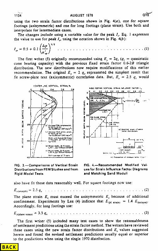
11; AUGUST 1978

using the two strain factor distributions shown in Fig. 4(u), one for square footings (axisymmetric) and one for long footings (plane strain). Use both and interpolate for intermediate cases.

The changes include using a variable value for the peak I,. Eq. I expresses the value to use for peak I,, using the notation shown in Fig. 4(b):

I,=O.5i-0.1 * ( ) l/2

. . . . . . . . . . . . . . . . * . . . . . . . . ., .

u:, (1)

The first writer (5) originally recommended using E, = 2q, (q, = quasistatic cone bearing capacity) with the previous fixed strain factor 0.6-28 triangle distribution. The new distributions now require modifications of this earlier recommendation. The original E, = 2 q, represented the simplest result that fit screw-plate text (axisymmetric) correlation data. But, E, = 2.5 q, would

CENTER LlNE VERTICAL STRAIN.%

FIG. 3.-Comparisons of Vertical Strain Distributions from FEM Studies and from Rigid Model Tests

FIG. 4.--Recommended Modified Val- ues for Strain Influence Factor Diagrams and Matching Sand Moduli

also have fit these data reasonably well. For square footings now use:

E F(sx,sym) = 2.5 q, . . . . . . . . . . . . . . . . . . . . . (2)

The plane strain E, must exceed the axisymmetric E, because of additional confinement. Experiments by Lee (4) indicate that E,,, rtrrinj = 1.4 E~axisym). Accordingly, for long footings use:

E s(plane slrmn! =3sq, . . . . . . . . . . . . . . . . . . . . . . . . . . .(3)

The first writer (5) included many test cases to show the reasonableness of settlement predictionsusing the strain factor method. The writers have reviewed these cases using the new strain factor distributions and E, values suggested herein and found the revised settlement predictions usually equal or superior to the predictions when using the single 1970 distribution.

GTE TECHNICAL NOTES i- 1135

C~NCLU~I~N~

The writers offer the following conclusions: (1) Use separate strain factor distributions for square and long footings, as shown in Fig. 4(u); (2) increase the peak value of strain factor as the net footing pressure increases, in accord with Fig. 4(b) and Eq. 1; and (3) multiply q, by 2.5 for square and 3.5 for long footings to obtain the equivalent sand modulus E, when using the Fig. 4(u) strain factor distributions.

APPENDIX.-REFERENCES

I.

2.

3.

4.

5.

Brown, P. T., and Gibson, R. E., “Rectangular Loads on Inhomogeneous Elastic Soil,” Journal oj the Soil Mechanics and Foundations Division, ASCE, Vol. 99. No. SMIO, Proc. Paper 10042, Oct., 1973. pp. 917-920. Duncan, J. M., and Chang, C-Y., “Nonlinear Analysis of Stress and Strain in Soils,” Journal of the Soil Mechanics and Foundations Division. ASCE. Vol. 96. No. SM5. Proc. Paper 7513, Sept., 1970, pp. 1629-1655. Hartman, J. P., “Finite Element Parametric Study of Vertical Strain Influence Factors and the Pressuremeter Test to Estimate the Settlement of Footings in Sand,” thesis presented to the University of Florida, at Gainesville, Fla., in 1974, in partial fulfillment of the requirements for the degree of Doctor of Philosophy. Lee, K. L., “Comparison of Plane Strain and Triaxial Tests on Sand.” Journal of rhe Soil Mechanics and Foundations Division, ASCE, Vol. 96, No. SM3, Proc. Paper 7276, May, 1970, pp. 901-923. Schmertmann, J. H., “Static Cone lo Compute Static Settlement Over Sand,” Journal of the Soil Mechanics and Foundations Division. ASCE. Vol. 96. No. SM3. Proc. Paper 7302, May, 1970, pp. 101 l-1043.

Documents

bartlett/CVEEN5305/Handout 6... · Created Date: 10/28/2015 5:49:07 PM