Baroclinic Tides at Fieberling Guyot: Evaluating the Ability

Baroclinic Tides at Fieberling Guyot: Evaluating the Ability to Simulate Velocities

Robin Robertson Lamont-Doherty Earth Observatory

Columbia University Palisades, New York 10964

USA Office (845) 365- 8527

fax (845) 365- 8157 [email protected]

Submitted to J. Atmos. Ocean Technology July 28, 2004

Robertson: Baroclinic tides at Fieberling Guyot: Evaluating the Ability to Simulate Velocities

2

ABSTRACT

Terrain-following ocean models are being used to simulate the baroclinic tides and to provide

estimates of the tidal fields to circulation and mixing studies. These models have successfully

reproduced elevations with most inaccuracies attributed to topographic errors; however, the

reproduction of either the baroclinic or barotropic velocity fields has not been as robust. Part of

the problem is the insufficiency of the observational data set in the simulated regions for

comparison. This problem can be addressed using a data set collected by K. M. Brink, J. M.

Toole, and C. C. Eriksen near Fieberling Guyot.

In order to evaluate the capability of the Regional Ocean Model System (ROMS) to simulate

tidal velocities, the combined tides of four constituents, M2, S2, K1, and O1 for the Fieberling

Guyot region were modeled. Several model parameters were varied in order to improve the

agreement with observations, including 1) bathymetry, 2) hydrography, 3) horizontal resolution,

4) vertical resolution (number of layers and layer spacing), and 5) the parameterization of

vertical mixing. The semi-diurnal baroclinic tides were replicated well with rms differences

between the model estimates and observations of 2.1 and 0.8 cm s-1 for the major axes for the M2

and S2 constituents, respectively. However the diurnal K1 baroclinic tides were not with rms

differences of 5.2 cm s-1. The most important factors were found to be the horizontal resolution

and the accuracy of the bathymetry. Finer horizontal resolution will improve the agreement

between model results and observations until the grid resolution reaches the accuracy of the

bathymetry. The vertical mixing parameterization was found to have minor effects on the

velocity fields, with most of the effects occurring within the benthic boundary layer; however, it

had dramatic effects on the estimation of the vertical diffusivity. The major axes of the tidal


3

ellipses and vertical momentum diffusivity observations were best replicated by the Large-

McWilliams-Doney and generic length scale version of the ?-? parameterization.

Key Words: Tides, Internal tides, baroclinic tides, internal waves, vertical mixing

parameterizations


4

1. Introduction

Recently, tides and internal waves have been recognized to play a significant role in ocean

mixing, (Munk and Wunsch, 1998; Garrett, 2003). Barotropic tides increase the benthic mixing

through higher benthic shear. They also interact with rough topography and generate baroclinic

tides, which induce vertical shear in the water column, leading to shear instabilities and mixing.

To fully understand and quantify the role that tides are playing in mixing, the baroclinic and

barotropic tidal fields must be known, particularly over rough topography and along the

continental shelf break. Although the barotropic tidal fields can be observed by satellite for M2,

S2, and K1 (Andersen 1995), only the semi-diurnal baroclinic tides are observable by satellite

(Ray and Mitchum, 1996). The diurnals cannot be resolved, because the repeat cycles of the

satellites are too close to their tidal periods (Ray and Mitchum, 1996). And these estimates

reflect only the surface signature not the mid-water column response, due to the limitations of

satellite imagery. Direct observation of the global baroclinic tidal fields, although desirable,

would be prohibitively expensive. An alternative method to determine baroclinic tidal fields is

modeling them for the rough topographic regions and along the continental shelves. Niwa and

Hibiya have modeled the baroclinic tides for the Pacific Ocean using a set of coarse grids in

order to estimate the baroclinic tidal energy (2001). Regionally, baroclinic tides have been

modeled in the Ross Sea by Robertson et al. (2003a; 2003b), over the Hawaiian Ridge by

Merrifield et al. (Merrifield et al., 2001; Merrifield and Holloway, 2002), and over the

Northwestern Australian Slope by Holloway (1996: 1997).

However for verification purposes, the modeling results should be evaluated using

observations as ground-truth and their limitations identified, since not all physical processes are

included and parameterizations are used in the mode to represent the unresolved processes. Due


5

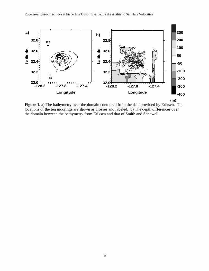
to an extensive set of observations for the Fieberling Guyot area collected by Noble, Ericksen,

Toole, Kunze, and Brink (Figure 1) (Noble et al., 1994; Ericksen 1998; Toole et al., 1997; Kunze

and Toole, 1997; and Brink,), it was selected for an eva luation of the capabilities of a baroclinic

tidal model. Since vertical mixing estimates are of interest and the sub-grid scale vertical mixing

is parameterized in this model, the effects of several different vertical mixing parameterizations

on the model velocity and vertical viscosity fields were evaluated.

Section 2 gives a quick description of the model and section 3 brief descriptions of the

different vertical mixing parameterizations and their implications on mixing. The baroclinic

tidal fields are evaluated and compared to observations in section 4, which also discusses a

sensitivity study evaluating different operating considerations. Section 5 evaluates the results

from using the different vertical mixing parameterizations. A summary is provided in section 6.

2. Model Description

a. The Model

When modeling regions with rough topography, it is preferable to use terrain-following

models, such as the Princeton Ocean Model (POM) or ROMS, since the coordinate system of

these models allows a more realistic representation of both the topography and surface and

benthic boundary layers with fewer vertical levels than are needed for equivalent z- level models.

Barotropic and baroclinic tides have been previously modeled using both POM and ROMS

(POM: Holloway, 1996; Robertson, 2001a; ROMS: R. Hetland, 2001 personal communication;

Robertson et al., 2003; Robertson, 2003). ROMS was used in this study and was chosen due to

the option of using more accurate baroclinic pressure gradient formulation (density Jacobian

scheme using monotonized cubic polynomial fits) (Ezer et al,. 2002) and inclusion of different

parameterizations for vertical mixing. No simulations were made with POM nor was any


6

attempt made to compare the performance of the two models. A comparison of the models has

been made for some applications by Ezer et al. (2002).

Using ROMS, different options are available for simulation of some of the physical

processes. The options used for the base case will be identified. For horizontal advection, third

order upstream differencing, Laplacian lateral diffusion along sigma surfaces (10 m2 s-1)

(Shchepetkin and McWilliams 2002) were used. As will be discussed later, a sensitivity study

was performed for several vertical mixing parameterizations (Table 1). However for the base

case, the Large-McWilliams-Doney (LMD) vertical mixing scheme was used (Large and Gent

1999). Flather radiative boundary conditions were implemented for the barotropic mode

velocities and flow relaxation boundary conditions for the baroclinic mode velocities and tracers.

Tidal forcing was implemented by setting elevations and velocities along all the open

boundaries, with the coefficients taken from a two-dimensional model of the region Egbert et

al.’s global inverse tidal model (OTIS) (Egbert and Erofeeva, 2002). Four major tidal

constituents were simulated, two semi-diurnals, M2 and S2 and two diurnals, K1 and O1. The

barotropic and baroclinic mode time steps were 8 s and 240 s, respectively, and the simulations

were run for 30 days, with hourly data from the last 15 days used for analysis. The time step was

reduced for the higher resolution simulations. The kinetic and potential energies stabilized

around 15 days, thus the first 15 days of simulated data was discarded.

b. Topography and Hydrography

The model domain (Figure 1) covered the Fieberling Guyot with a spacing of 2 km in the

North-South and East-West direction and 24 vertical levels. The nominal bathymetry was taken

from Smith and Sandwell (1997) and a more detailed bathymetry was supplied by Eriksen

(personal communication, 2003). No smoothing was performed on the water depths.


7

Initial potential temperature, ?, and salinity, S, fields were assembled from Levitus (1994).

The model elevation and velocities were initialized with the geostrophic velocities associated

with the initial hydrography as determined from a 30-day simulation without tidal forcing.

c. Model Outputs

Elevation, ? , and depth-independent velocities, U2 and V2, are produced by the two-

dimensional (barotropic) mode of the model and ?, S, and depth-dependent velocities, U3, V3,

and W3, by the three-dimensional (baroclinic) mode. The depth-dependent velocities comprise

the complete velocity from the equations of motion, and do not have the depth- independent

portion removed. Foreman’s tidal analysis routines were used to analyze these fields (Foreman

1977; 1978).

3. Vertical Mixing Parameterizations

The processes causing vertical mixing cover a wide-range of scales, from a few cm for salt

fingers to over a thousand meters for deep convective mixing. Many of these scales are not

resolvable for either sigma or z coordinate models without an excessive number of levels. To

address this problem, vertical mixing is parameterized in the models to represent the unresolved

sub-grid scale mixing. Consequently, the vertical mixing predicted by the model is completely

dependent upon the parameterization being used.

There have been many different approaches to estimating vertical mixing and several of the

parameterizations have been included in ROMS. The most predominantly used schemes are 1)

Pacanowski-Philander (PP) turbulence closure scheme (Pacanowski and Philander, 1981), 2) an

N-1 based scheme (BVF) (Gargett and Holloway, 1984), 3) Mellor-Yamada (MY) 2.5 level

turbulence closure scheme (Mellor and Blumberg, 1985), 4) Large-McWilliams-Doney (LMD)

scheme (Large and Gent, 1999), 5) a modification to LMD (LMD-SSCW) (Smyth et al., 2002), 6)


8

Lamont Ocean Atmospheric-Mixed-Layer Model (LOAM) scheme, which is based on PP (PP-

LOAM, 2002), and 7) generic length scale scheme (GLS), which can reproduce MY (? -? l), ?-? ,

?-?, and other ?-? based schemes (Umlauf and Burchard, 2003). All of these schemes, except

the second, use the gradient Richardson number (Ri) to determine spatially and temporally varing

vertical mixing coefficients for momentum (K?) and tracers (K? ), although the LMD and GLS

schemes are not completely dependent on Ri. In these parameterization schemes, Ri is used as a

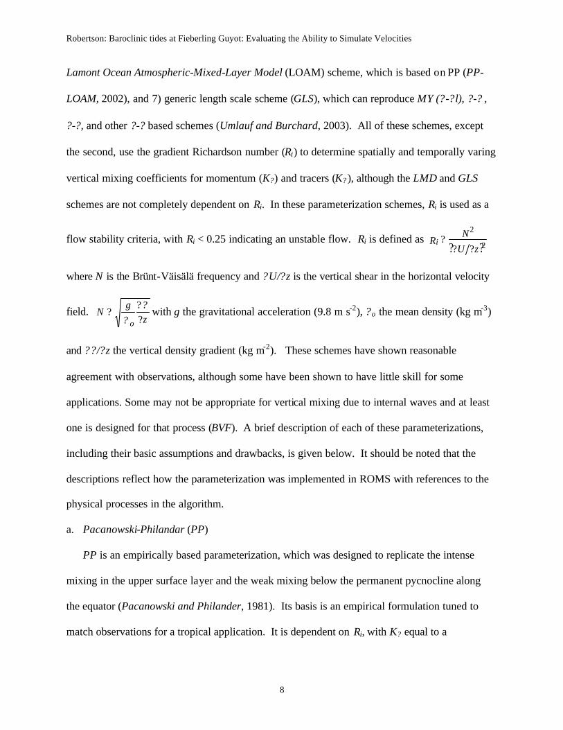
flow stability criteria, with Ri < 0.25 indicating an unstable flow. Ri is defined as ? ?zU

NRi

???

2

2

where N is the Brünt-Väisälä frequency and ?U/? z is the vertical shear in the horizontal velocity

field. z

gN

o ??

??

?with g the gravitational acceleration (9.8 m s-2), ? o the mean density (kg m-3)

and ?? /? z the vertical density gradient (kg m-2). These schemes have shown reasonable

agreement with observations, although some have been shown to have little skill for some

applications. Some may not be appropriate for vertical mixing due to internal waves and at least

one is designed for that process (BVF). A brief description of each of these parameterizations,

including their basic assumptions and drawbacks, is given below. It should be noted that the

descriptions reflect how the parameterization was implemented in ROMS with references to the

physical processes in the algorithm.

a. Pacanowski-Philandar (PP)

PP is an empirically based parameterization, which was designed to replicate the intense

mixing in the upper surface layer and the weak mixing below the permanent pycnocline along

the equator (Pacanowski and Philander, 1981). Its basis is an empirical formulation tuned to

match observations for a tropical application. It is dependent on Ri, with K? equal to a


9

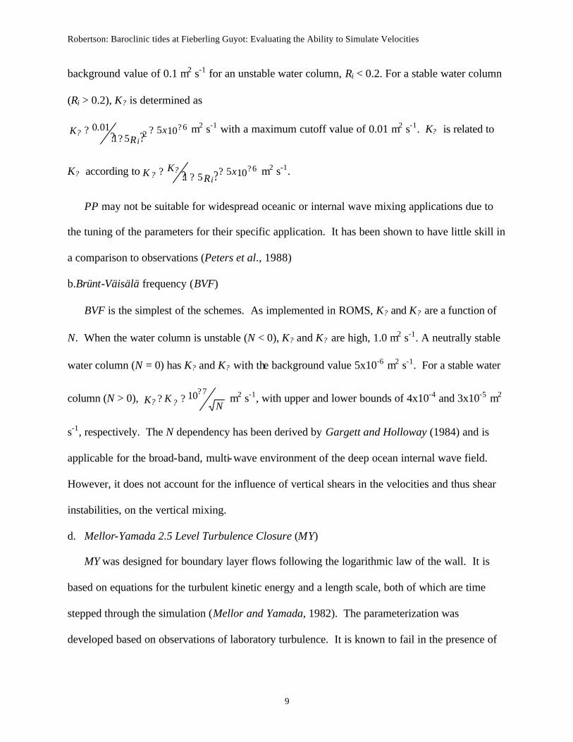
background value of 0.1 m2 s-1 for an unstable water column, Ri < 0.2. For a stable water column

(Ri > 0.2), K? is determined as

? ? 10551

01.0 62

???

? xR

Ki

? m2 s-1 with a maximum cutoff value of 0.01 m2 s-1. K? is related to

K? according to ? ? 105516???? x

RKK

i?? m2 s-1.

PP may not be suitable for widespread oceanic or internal wave mixing applications due to

the tuning of the parameters for their specific application. It has been shown to have little skill in

a comparison to observations (Peters et al., 1988)

b.Brünt-Väisälä frequency (BVF)

BVF is the simplest of the schemes. As implemented in ROMS, K? and K? are a function of

N. When the water column is unstable (N < 0), K? and K? are high, 1.0 m2 s-1. A neutrally stable

water column (N = 0) has K? and K? with the background value 5x10-6 m2 s-1. For a stable water

column (N > 0), N

KK 10 7???? ? m2 s-1, with upper and lower bounds of 4x10-4 and 3x10-5 m2

s-1, respectively. The N dependency has been derived by Gargett and Holloway (1984) and is

applicable for the broad-band, multi-wave environment of the deep ocean internal wave field.

However, it does not account for the influence of vertical shears in the velocities and thus shear

instabilities, on the vertical mixing.

d. Mellor-Yamada 2.5 Level Turbulence Closure (MY)

MY was designed for boundary layer flows following the logarithmic law of the wall. It is

based on equations for the turbulent kinetic energy and a length scale, both of which are time

stepped through the simulation (Mellor and Yamada, 1982). The parameterization was

developed based on observations of laboratory turbulence. It is known to fail in the presence of


10

stratification (Simpson et al., 1996) and was not designed for internal wave mixing (Large and

Gent, 1999). MY is also computationally intensive.

e. Large-McWilliams-Doney KP profile (LMD or KPP)

LMD separates mixing physics into three primary physical processes: local Ri instabilities

due to resolvable vertical shear, internal wave, and double diffusion. The total vertical mixing

coefficient for momentum, K?, is a sum of coefficients resolvable vertical shear and internal

waves KKK is ?? ??? , while the total vertical mixing coefficient for tracers, K? , is a sum of

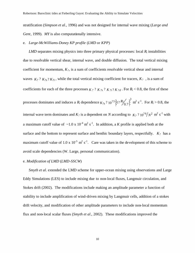
coefficients for each of the three processes KKKK dis ??? ???? . For Ri < 0.8, the first of these

processes dominates and induces a Ri dependence ????

?? ?? ?

7.01103

3 RK is? m2 s-1. For Ri > 0.8, the

internal wave term dominates and K? is a dependent on N according to NK 2610??? m2 s-1 with

a maximum cutoff value of ~1.0 x 10-4 m2 s-1. In addition, a K profile is applied both at the

surface and the bottom to represent surface and benthic boundary layers, respectfully. K? has a

maximum cutoff value of 1.0 x 10-5 m2 s-1. Care was taken in the development of this scheme to

avoid scale dependencies (W. Large, personal communication).

e. Modification of LMD (LMD-SSCW)

Smyth et al. extended the LMD scheme for upper-ocean mixing using observations and Large

Eddy Simulations (LES) to include mixing due to nonlocal fluxes, Langmuir circulation, and

Stokes drift (2002). The modifications include making an amplitude parameter a function of

stability to include amplification of wind-driven mixing by Langmuir cells, addition of a stokes

drift velocity, and modification of other amplitude parameters to include nonlocal momentum

flux and nonlocal scalar fluxes (Smyth et al., 2002). These modifications improved the


11

performance almost to that of the LES, although the simulations focused on the upper 100 m

(Smyth et al., 2002).

f. LOAM modifications to PP (PP-LOAM)

A modification in the parameterization values, PP-LOAM, has been developed at Lamont-

Doherty Earth Observatory (LDEO) for the more generalized ocean (LOAM, 2002). This

parameterization may be more appropriate for shallow coastal regions and regions with fronts.

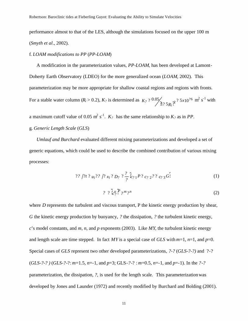
For a stable water column (Ri > 0.2), K? is determined as ? ? 105

5105.0 6

2??

?? x

RK

i? m2 s-1 with

a maximum cutoff value of 0.05 m2 s-1. K? has the same relationship to K? as in PP.

g. Generic Length Scale (GLS)

Umlauf and Burchard evaluated different mixing parameterizations and developed a set of

generic equations, which could be used to describe the combined contribution of various mixing

processes:

? ?GccPcDxut ii 321 ???? ????? ????????? (1)

? ? ??? ?nmo p

c? (2)

where D represents the turbulent and viscous transport, P the kinetic energy production by shear,

G the kinetic energy production by buoyancy, ? the dissipation, ? the turbulent kinetic energy,

c’s model constants, and m, n, and p exponents (2003). Like MY, the turbulent kinetic energy

and length scale are time stepped. In fact MY is a special case of GLS with m=1, n=1, and p=0.

Special cases of GLS represent two other developed parameterizations, ?-? (GLS-?-?) and ?-?

(GLS-?-? ) (GLS-? -?: m=1.5, n=-1, and p=3; GLS-? -? : m=0.5, n=-1, and p=-1). In the ? -?

parameterization, the dissipation, ?, is used for the length scale. This parameterization was

developed by Jones and Launder (1972) and recently modified by Burchard and Bolding (2001).


12

In the ?-? parameterization, the rate of dissipation of energy per unit volume and time, ? , is

used as the length scale, with ? ? kc0 4

?

?? ? where c0? again is a constant. In order to use this

scheme in stratified flows, buoyancy was included by Umlauf et al. (2003). An additional

scheme (GLS-gen) with m=1, n=-0.67, and p=1 was developed by Umlauf and Burchard (Warner

et al., 2003). GLS has been implemented in ROMS. For this study, the GLS parameters used

were those for the four GLS schemes compared by Warner et al. (2003). These four GLS

schemes have been compared for various applications including steady barotropic flow, wind-

induced surface mixed layer deepening in a stratified fluid, oscillatory stratified pressure-

gradient driven flow, and an estuarine situation (Warner et al., 2003). The GLS-MY performed

poorly in the estuarine flow and the performance of the other three, GLS-?-?, GLS-?-? , and

GLS-gen, were similar with slight differences (Warner et al., 2003). They were unable to

ascertain which of these three GLS-?-?, GLS-?-? , and GLS-gen, was more realistic (Warner et

al., 2003).

4. Simulating Baroclinic Tides

a. Three-dimensional Tidal Fields

The major axes of the tidal ellipses of the depth-dependent velocities, U3 and V3, were

determined for the four constituents, M2, S2, K1, and O1. The results of the base case will be

described here. Results of the sensitivity study will follow in subsequent sections. The semi-

diurnal constituents, M2 and S2, behaved similarly; consequently M2 will be taken as

characteristic of the semi-diurnal response.

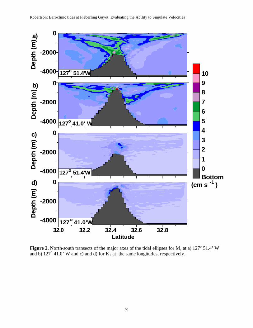
As predicted by linear internal wave theory, the semi-diurnal constituents generated interna l

tides over the crown and flanks of Fieberling Guyot (Figure 2a-b for M2). The internal tides


13

propagated away from the guyot following internal wave characteristics. Linear internal wave

theory predicted a barotropic response for the diurnal constituents since the location is poleward

of the diurnal critical latitudes (latitude where the inertial frequency equals the tidal frequency).

The diurnal response was nearly barotropic with slight baroclinic tides generated in the midwater

column and at the bottom over the crown of the guyot and very little propagation (Figure 2c-d

for K1). The diurnal response was much smaller than the semi-diurnal with peak values of 4 cm

s-1 and 10 cm s-1, respectively.

b.Observations

Fieberling Guyot was the focus of an intense observational study of tidal interactions with

seamounts and guyots topography, such as continental shelf waves and internal waves. Over

Fieberling Guyot, nine moorings with current meters or an ADCP were situated along two radial

arms (Figure 1) (Brink 1995). A pilot study the year before provided an additional mooring, P,

(Noble et al. 1994). The ten moorings yielded forty-four current observation locations/depths.

Three moorings, F3, F4, and F5, were situated close together and in the model comparisons, they

occupy the same grid cell. They were treated as one site even though their exact locations were

used when estimating the model values. Additionally, hydrographic survey and vertical viscosity

measurements were collected in the spring of 1991 by Kunze and Toole (1997). And a high

resolution bathymetric survey was performed (Eriksen 1991). This observational data set was

used both for initial conditions for the model and as ground-truth for the model estimates.

c. Validation of Model Results Against Observations

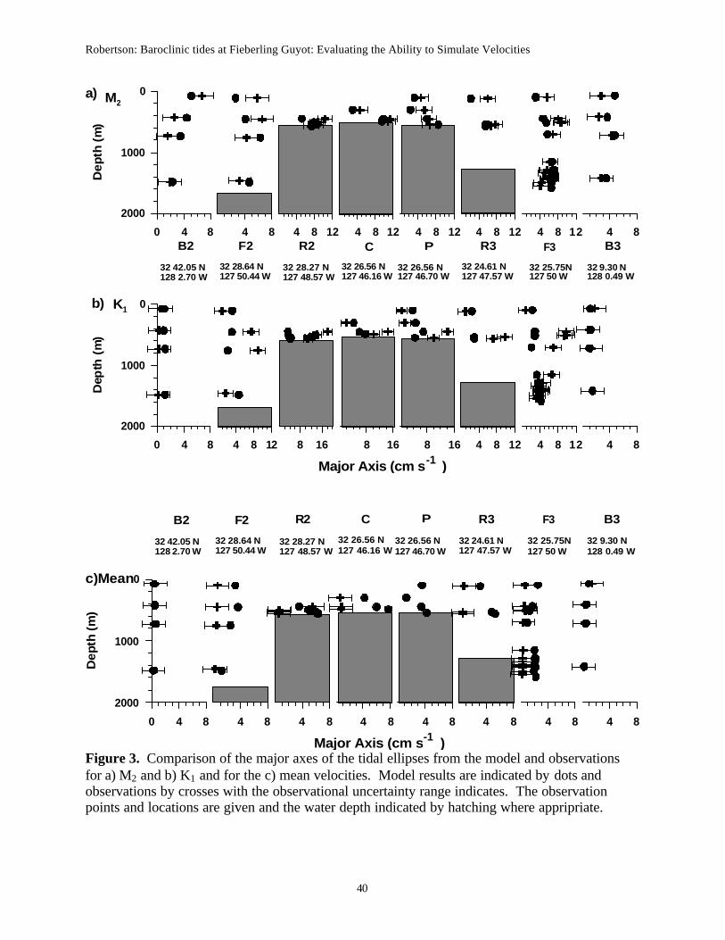
For the base case, the model estimates agreed well with the observations for the semi-diurnal

constituents with twenty-six and all estimates within the observational uncertainty (1.7 cm s-1)

for M2 and S2, respectively (Figure 3a). However, the agreement for the diurnals was poor for K1


14

with twenty-two of the estimates falling outside the observational uncertainty (Figure 3b). Only

seven of the estimates for O1 fell outside the observational uncertainty. Rms differences for the

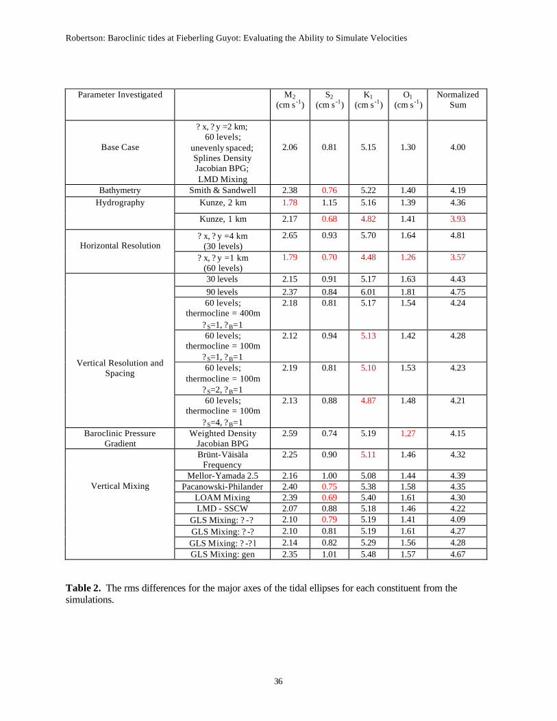
major axes were 2.06, 0.81, 5.15, and 1.30 cm s-1 for M2, S2, K1, and O1, respectively. The lower

rms differences for S2 and O1 reflect the lower observational velocities.

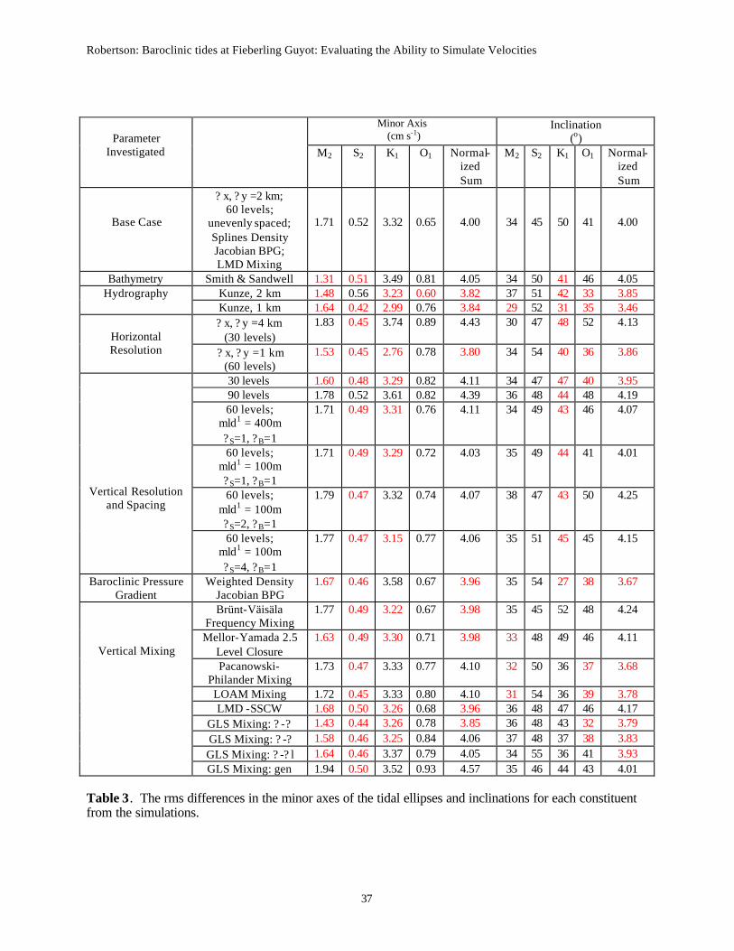
The rms difference reflects only the difference in the amplitude of the ellipse. The

orthogonal velocities and the angle the velocities impinge on the slopes are also important. Rms

differences were determined for the minor axes of the tidal ellipses and the inclination to

evaluate these factors. The rms differences for the minor axes were 1.71, 0.52, 3.32, and 0.65

cm s-1 for M2, S2, K1, and O1, respectively. The rms values for the minor axes are less than those

for the major axes, reflecting the smaller magnitudes. For the inclination, rms differences were

quite high, 34, 45, 50, and 41o for M2, S2, K1, and O1, respectively. High rms differences for the

inclination often occur when the major and minor axes have similar magnitudes, nearly circular

ellipses. With nearly circular ellipses, small errors can switch the minor axes to being the major

axis and vice versa, introducing a 90o shift into the inclination. And nearly circular ellipses are

typical for both the deep ocean and regions near the critical latitude (the latitude where the

inertial frequency equals the tidal frequency). Nearly circular ellipses occurred for some of the

lower magnitude values, particularly for K1.

Large mismatches occurred for K1 over the guyot. The model responds barotropically for the

diurnal constituents; however, the observations show a baroclinic response (Figure 3b). The

model response follows internal wave theory. Fieberling Guyot is poleward of the diurnal

critical latitudes (28o and 30o), so linear internal wave theory predicts a barotropic response

there. Thus, how does the baroclinic response enter the observations? Kunze and Toole. (1997)

postulated that relative vorticity of the tidal mean flow combines with the planetary vorticity to


15

shift the effective critical latitude poleward of Fieberling Guyot, so baroclinic tides are

generated. However, this does not happen in the model results. At this resolution, the model

does not estimate the mean velocities sufficiently (Figure 3c) to reduce the vorticity and as a

result the diurnal response is barotropic. The model overpredicts the mean ve locity for most

(twenty-six of thirty-six) of the sites. Note that the mean velocities were not determined for site

P, since the time series were unavailable.

The mean velocities were different than those estimated by Beckmann and Haidvogel (1997).

Beckmann and Haidvogel modeled the circulation around Fieberling Guyot forced by a generic

diurnal tide and reasonably simulated the mean flow. They used smoothed topography on a

nominally 0.5 km grid. But they did not do a quantitative comparison against observational data.

Since the models are similar, the different response is probably either the forcing or the

horizontal resolution.

There are many sources for disagreement between the model estimates and the observation.

Sometimes, there are errors in the observations and observations at nearby locations or nearby

depths on the same mooring will differ greatly. Velocity disagreement can occur when the

model depth for a location is different than the corresponding observed water depth, especially

when the depth for either the model estimate or the observation is in the boundary layer for one

but not the other. Differences in the background flow can lead to differences between the model

and the observations. The model simulations here have no background flow, but the

observations often do. Small, sub-grid scale features ignored by the model, but can influence the

observed fields.

d. Sensitivity study


16

In order to evaluate the effects of inputs and parameters on the modeling capability, a

sensitivity study was made for different bathymetries, hydrographies, horizontal and vertical

resolutions, and vertical spacing (Table 1). Effects of the vertical mixing parameterization were

also investigated and are discussed in section 5. Model performance was evaluated using rms

differences for the major and minor axes of the tidal ellipses and the inclination for each

constituent (Tables 2 and 3). To facilitate the comparison between simulations, a normalized

sum of the rms differences was determined. This normalized sum combines values for each

simulation normalized by the corresponding value for the base case.

1) Bathymetric effects

To investigate the effect of the accuracy of the bathymetry on the performance of the model,

a simulation was performed using the Smith and Sandwell bathymetry at the same resolution as

the bathymetry from Eriksen. Although the same resolution was used, the Smith and Sandwell

bathymetry is coarser and some of the finer features in the Eriksen are smoothed out (Figure 1b).

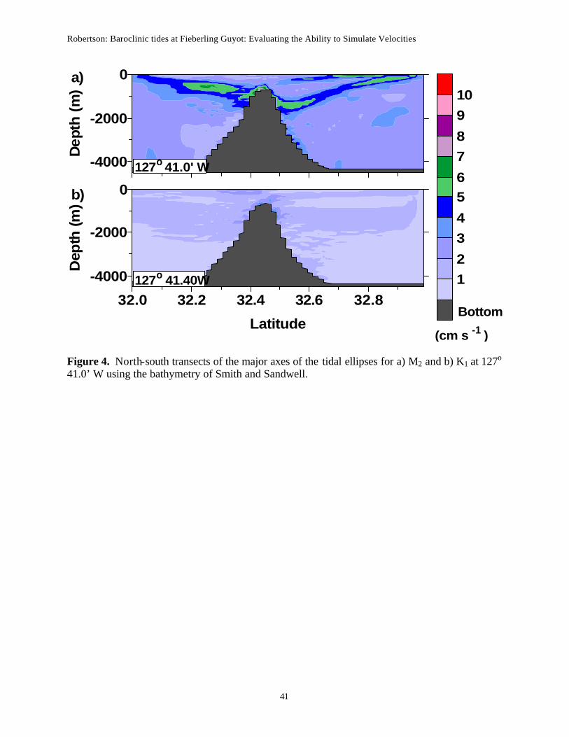
For the semi-diurnal constituents, the baroclinic response was greater with the Eriksen

bathymetry (Figure 2) than with the Smith and Sandwell bathymetry (Figure 4). The rms

differences for the major axes were slightly higher for M2, K1, and O1 and slightly lower for S2

for the Smith and Sandwell bathymetery (Table 2). Although the simulation with the Smith and

Sandwell bathymetry replicated the minor axes for the semidiurnal constituents better than with

the Eriksen bathymetery with lower rms values (Table 3), the Eriksen bathymetery simulation

replicated the overall currents better as reflected in the lower value for the normalized sum of the

rms differences for both the major and minor axes.

2) Hydrographic effects


17

For the base case, the initial hydrography was taken from a climatic atlas (Levitus, 1994).

Since baroclinic tidal generation is dependent on the hydrography, a simulation was performed

using the hydrography measured by Kunze and Toole (1997). Profiles for observed potential

temperature and salinity were optimally interpolated to the grid cell locations and depths. The

rms differences for the major axes were lower with the realistic hydrography for M2, but higher

for S2 and O1 (Table 2). The rms differences were generally lower for the major and minor axes

and inclination with the realistic hydrography as reflected in the lower normalized sums (Tables

2 and 3). A high resolution simulation was performed using the realistic hydrography on a 1 km

grid. Although this 1 km, realistic hydrography simulation performed better than the base case

with lower normalized sums for all tidal ellipse parameters, it did not perform better than the 1

km simulation with Levitus hydrography with respect to the major axes (Tables 2 and 3).

3. Horizontal resolution effects

To investigate the effects of the horizontal resolution, simulations were performed using the

Eriksen bathymetry, but with grid resolutions of 4 km, 2 km, and 1 km in both horizontal

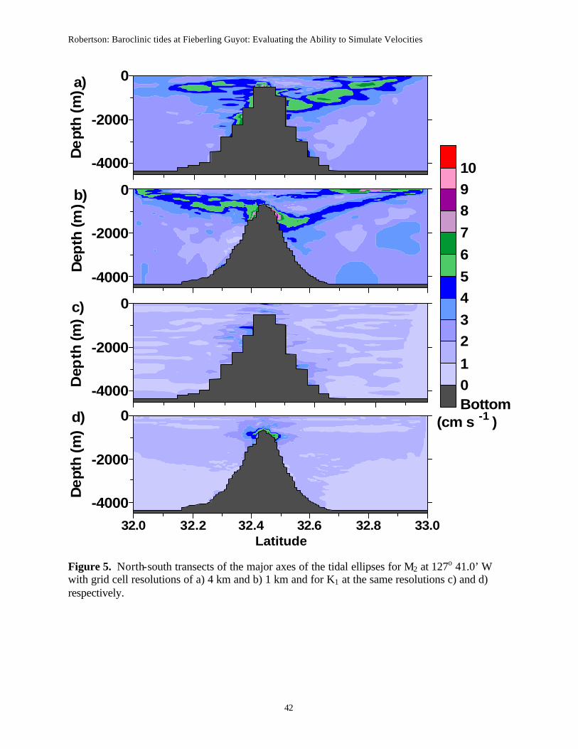
directions (Table 1). With the higher resolution bathymetry, more generation occurred along the

rim and flank for all constituents (Figure 5). The model results best replicated the observations

with the 1 km resolution with lower rms differences for the major and minor axes for all

constituents (Tables 2 and 3). The normalized sums of the rms differences for all constituents

was significantly lower for the 1 km resolution than for the base case, 3.57, 3.80, and 3.86 for the

major axes, minor axes, and inclination, respectively, compared to 4.00 for the base case. The

improvements for the semi-diurnals occurred over the flank, rim, and center of the guyot.

Excessively strong mean currents, present in the coarse resolution simulation, were reduced in

the higher resolution simulations. The estimates of the mean currents improved dramatically


18

over the flank and the center, although the observed mid-water column peak at F3 and high

benthic velocities at R2 were not reproduced. Correspondingly, for the diurnal constituents, the

observed mid-water column peaks at F2 and F3 and the high benthic values at R2, R3, C and P

were not reproduced (Figure 5c-d). The generation of baroclinic tides shifted to shallow depths

on the guyot with the finer resolution for the semi-diurnals (Figure 5a-b). For the diurnals,

baroclinic tidal generation increased both in amplitude and extent as the resolution increased

(Figures 2b and 5c-d). With the finer resolution, baroclinic tidal generation was also more

localized with large major axes occurring in isolated spots. Although better performance might

have been attained by higher resolution simulations, 0.5 km, such a high resolution simulation

was not done since it exceeded the resolution of the bathymetry, ~1 km.

4) Vertical resolution and spacing effects

Vertical resolution depends not only on the number of levels, but also on the spacing of the

levels. The spacing of the levels in ROMS is determined by three parameters: the mixed layer

depth, ?S, and ?B. ?S, and ?B create closely spaced levels at the surface and bottom, respectively,

in order to resolve the dynamics in the boundary layers more effectively. Simulations were

performed with 30 and 90 levels, as a decrease and an increase in the layers over the 60 levels

used in the base case. The spacing parameters were not changed for these simulations. The

spacing parameters were changed for additional cases using 60 levels, six of which are shown in

Tables 2 and 3. With only 30 levels, the baroclinic tidal generation decreased and the

disagreement between the observations and model estimates slightly increased. The changes

were small however, with rms differences for the major axes that were only slightly larger.

There was no effective change in the baroclinic generation or improvement in the agreement

with the increase to 90 levels. Changing the level spacing can effectively increase the number of


19

levels for regions where variables change rapidly, like the surface and the bottom. Although the

performance improved for some of the vertical spacings for K1, the overall model performance

was not improved either by deepening the mixed layer thickness or modifying the spacing in the

surface and boundary layers as seen by the higher normalized sum of the rms differences for all

ellipse parameters (Tables 2 and 3).

5. Baroclinic Pressure Gradient

The baroclinic pressure gradient is the term in the Navier-Stokes equations that generates the

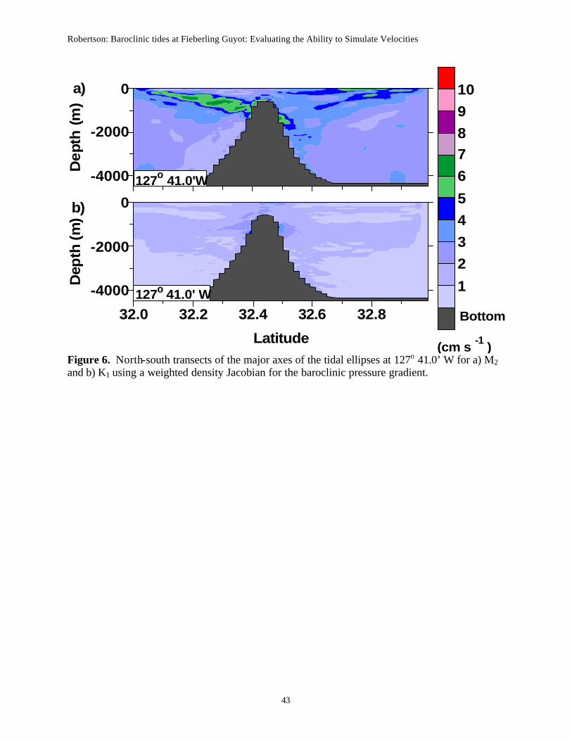
baroclinic tides and internal waves. A simulation was performed with a weighted density

Jacobian numerical method for determining the baroclinic pressure gradient. Although they had

similar responses (Figures 2 and 6), more baroclinic generation occurred with the splines density

Jacobian. Rms differences were lower for the major axes for the splines density Jacobian and

rms differences were lower for the for the semidiurnal minor axes and diurnal inclinations for the

weighted density Jacobian; however, the improvement in the minor axis and inclination did not

out weigh the worse performance in the major axes.

5. Vertical Mixing Parameterization Effects

Performance of different vertical mixing schemes has been the subject of much recent

discussion (Umlauf et al., 2003; Warner et al., 2003) and the scheme with the best performance

for one application may not perform the best for another. For example, in an application of tides

in the Irish Sea, GLS ?-?l and GLS: ?-? performed similarly (Burchard et al, 1998); however, in

an estuarine application, GLS ? -? l performed poorer than GLS: ? -? or GLS: ?-? (Warner et al.,

2003). GLS: ?-? has been said to be more accurate than LMD, but LMD is less computationally

intensive (Smyth et al., 2002).


20

The performance of vertical mixing parameterization schemes for the application of

baroclinic tides over Fieberling Guyot was evaluated. Ten different parameterizations were

investigated for their effects on both the velocity fields and the vertical mixing coefficient as

estimated by the model (see section 3 for a brief description of their characteristics).

a. Effects on Velocities

Vertical mixing controls the dissipation of energy and the reduction velocities in the benthic

boundary layer and the dissipation of the beams of internal tidal energy and the distance the

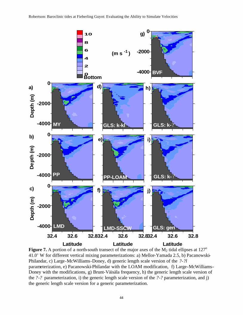
internal tidal beams propagate. The differences between the velocity fields of the ten vertical

mixing parameterizations were minor and occurred primarily near the bottom and near the

internal tidal beams (Figure 7). GLS: ? -? l had less internal tidal generation and smaller major

axes of the tidal ellipses over the flank than the other schemes (Figure 7). MY, BVF, LMD, PP-

LOAM, and LMD-SSCW had more generation with patches of larger major axes near the flanks

of the seamount than the others (Figure 7). Rms differences for the ellipse parameters indicate

that the best match with the observations occur with LMD and GLS: ?-? (Table 2). LMD had

the lowest rms differences for the major axes with GLS: ?-? only slightly higher. GLS: ?-? had

lower rms differences for the minor axes and inclination as indicated by the normalized sums

semi-diurnal constituents (Table 3). The normalized sum for the GLS: ?-? were low enough to

offset the slightly higher major axes so that for the performance of the two schemes can be

considered roughly equivalent with respect to the velocities.

b. Effects on the Vertical Diffusivities

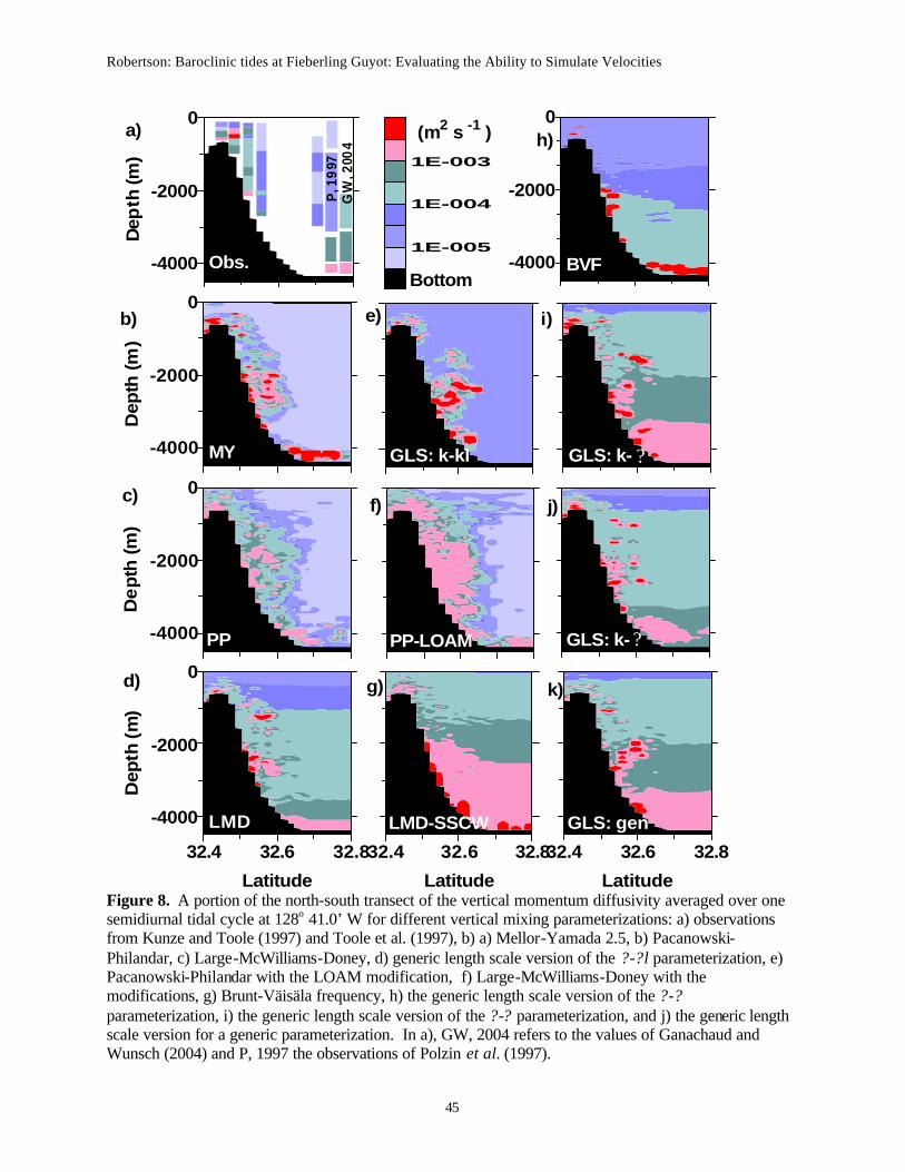
Observed vertical diffusivities for this area showed background values of 1-5 x10-5 m2 s-1 in

the upper 1000 m with peaks over 5x10-3 m2 s-1 in the regions of internal wave shear (Kunze and

Toole, 1997) (Figure 8a). Polzin et al.’s observations in the Brazil Basin suggest values of 10-3


21

m2 s-1 for roughly the 250 m above the bottom, 10-4 m2 s-1 above that level to 1000 m above the

bottom and a background value of 10-5 m2 s-1 in the upper 1000 m (1997).

Although the differences in the velocity fields for the vertical mixing parameterizations were

minor, the model estimates for the vertical diffusivities were quite varied for both the

background value and the response to the shear associated with the internal tide. It should be

noted that the vertical momentum diffusivities are time dependent through both the stratification

and the shear. The values in Figure 8 are averaged over one semidiurnal period. LMD, LMD-

SSCW, GLS: ?-? ., GLS: ?-?, and GLS: gen had a vertical gradient in the background vertical

momentum diffusivity, with larger values near the bottom and smaller values near the surface

(Figures 8d, 8g, 8i, 8j, and 8k). BVF also had a vertically varying background vertical

momentum diffusivity, but of a smaller magnitude (Figure 8h). The background values for these

schemes were greater than 5x10-4 m2 s-1, but basically agree with the general, bulk values

determined by Ganachaud and Wunsch (2004) and those observed by Polzin et al. (1997)

(Figure 8a). The background values for MY, PP, and PP-LOAM were uniform throughout the

water column and less than 1x10-5 m2 s-1 (Figures 8b, 8c, 8f), which agree with the observed

background value of Kunze and Toole (1997) (Figure 8a). GLS: ?-?l also had a uniform

background value, but it was higher, ~ 5 x10-5 m2 s-1. All of the schemes except for PP, PP-

LOAM, and BVF showed a patch of vertical momentum diffusivities greater than 1x10-3 and

peaks greater than 5x10-3 m2 s-1in response to the shear from the internal tides near the flank of

the guyot and radia ting along the ray of high major axes. (Figure 8). Values of these magnitudes

were observed over the peak and the flank of the guyot (Figure 8a). The background values of

LMD-SSCW were quite high over the bottom 2000 m and obscured the patch of high vertical

momentum diffusivities. The background value was also high at the surface for LMD-SSCW.


22

This is believed to be due to the enhanced mixing in the profile applied both at the surface and

the bottom. This enhanced mixing improved performance for some applications, but not this

one. PP had isolated spots vertical diffusivities reaching over 1x10-3 m2 s-1 (Figure 8c) and PP-

LOAM had a large patch of vertical diffusivities greater than 1x10-3 m2 s-1 (Figure 8f). PP and

PP-LOAM are sensitive to scaling factors and the turbulence did not scale to provide as much

mixing as the other schemes for PP and mixing over a broader area for PP-LOAM. BVF had

isolated spots of elevated vertical diffusivities in response to the internal tides (Figure 8h), but

they were adjacent to the guyot, but not radiating away (Figure 8a). This reflects the N

dependency of the scheme. Mixing will reduce the stratification, lowering N and increasing K?.

This relationship also is seen in the background values for BVF, with lower K? in the more

stratified upper ocean. Over the top of the guyot, MY, LMD, GLS: ?-? , and GLS: ?-? best

reproduced the observed vertical momentum diffusivities.

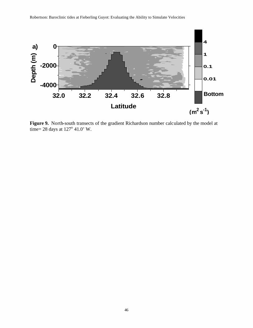
Why do the responses of the different vertical mixing parameterizations vary so much? A

map of the inverse gradient Ri for the same time as the vertical diffusivities gives some insight

(Figure 9), since most of them are gradient Ri based. A large patch of where the water column is

nearly unstable hugs the flank of Fieberling Guyot with Ri < 1.0 (inverse Ri >1) and patches

occur with unstable conditions Ri < 0.25 (inverse Ri >4). This patch coincides with the regions

of high diffusivities for all schemes except BVF, which is not gradient Ri based. Small patches

with unstable gradient Ri also occur near the peak of the guyot (Figure 9). Generally, the

gradient Ri values increase rapidly away from the guyot until a background value is reached,

indicating an increasingly more stable water column further away from the guyot (Figure 9).

The Ri based schemes reflected this in their vertical diffusivity estimates.


23

Differences also appear in the benthic boundary values. The values for GLS: ?-? decrease

near the bottom as the shear is reduced in the benthic boundary layer (Figure 8j). Other schemes

compensate for this reduction and do not show a reduction in the value near the bottom.

Finally, the big question of which scheme performs the best. Although the observations at

this site do not support the high vertical varying background values, the best match based on the

rms differences for the major axes occurred for LMD and GLS: ? -? , both of which had strong

vertical background gradients. The background gradient of the vertical momentum viscosities is

supported by the general observational estimates of Ganachaud and Wunsch (2004) (Figure 8a)

and Polzin et al. (1997). LMD replicates these observed patterns of Ganachaud and Wunsch and

Polzin et al. better than GLS: ?-? . (Figure 8). Therefore, the best performers appear to be LMD

and GLS: ?-? ., with LMD performing slightly better. These two schemes have the lowest rms

differences for the major axes, and replicate the observed vertical momentum diffusivities than

the others.

6. Summary

The capability of ROMS to simulate the baroclinic tides was evaluated in a sensitivity study that

investigated the impact of some of the inputs, resolution, and some parameterizations on the

performance. For the best case, the model replicated the baroclinic velocities for the semi-

diurnal constituents with rms differences for the major axes of 1.8 and 0.7 cm s-1 for M2 and S2,

respectively and for the diurnal constituents to 4.5 and 1.3 cm s-1 for K1 and O1, respectively.

Since Fieberling Guyot is poleward of the diurnal critical latitudes, linear internal wave theory

does not predict a baroclinic response and the model followed this response. However, the

observations show a baroclinic response for the diurnal constituents, which is not replicated by

the model. Kunze and Toole hypothesized that the tidally- induced mean current reduces the


24

vorticity enough to allow baroclinic waves and this is what is seen in the observations (1997).

The model does not reproduce the tidally induced mean velocity sufficiently to reduce the

vorticity and as a result only a diurnal barotropic response occurs.

Several model parameters were varied in order to improve the agreement with observations,

including 1) bathymetry, 2) hydrography, 3) horizontal resolution, 4) vertical resolution (number

of layers and layer spacing), and 5) the parameterization of vertical mixing. The most important

factors were found to be the horizontal resolution and the accuracy of the bathymetry. Finer

horizontal resolution improves the agreement between model results and observations until the

grid resolution reaches the accuracy of the bathymetry. The vertical mixing parameterization was

found to have minor effects on the velocity fields, but dramatic effects on the estimation of the

vertical diffusivity. Diffusivity observations were best replicated by the LMD paramterization of

vertical mixing with also good performance by the generic length scale method of applying the

?-? parameterization.

Acknowledgements:

Thanks are due to Marlene Noble, Charles Eriksen, John Toole, Eric Kunze, and Kenneth

Brink for supplying me with the data for Fieberling Guyot. Valuable information and insight

into the vertical mixing parameterizations was gained during discussions with William Large and

I am grateful for his input. This study was funded by (Office of Polar Programs) OPP grant

OPP-00-3425 of NSF. This is Lamont publication ????. Any opinions, findings, and

conclusions or recommendations expressed in this material are those of the authors and do not

necessarily reflect the views of the National Science Foundation.


25

References

Andersen, O. B., 1995, Global ocean tides from ERS 1 and TOPEX/Poseidon altimetry, J.

Geophys. Res.,100, 22,249-22,259.

Beckmann, A., and D. B. Haidvogel, 1997, A numerical simulation of flow at Fieberling Guyot,

J. Geophys. Res.,102, 5595-5613.

Brink, K. H., 1991, Coastal-trapped waves and wind-driven currents over the continental shelf,

Ann. Rev. Fluid Mech., 23, 399-412.

Brink, K. H., Tidal and lower frequency currents above Fieberling Guyot, J. Geophys. Res., 100,

10,817-10,832, 1995.

Burchard, H. and K. Bolding, 2001, Comparative analysis of four second-moment turbulence

closure models fo the oceanic mixed layer, J. Phys. Oceanogr., 31, 1943-1968.

Burchard., H., O. Petersen, and T. P. Rippeth, 1998, Comparing the performance of the Mellor-

Yamada and the k-? two-equation turbulence models, J. Geophys. Res., 103, 10,54371-

10,554.

Cummins, P. F., L.-Y-. Oey, 1997, Simulation of barotropic and baroclinic tides off northern

British Columbia, J. Phs. Oceanog., 27, 762-781.

Egbert, G. D., A. F. Bennett, and M. G. G. Foreman, 1994, TOPEX/Poseidon tides estimates

using a global inverse model, J. Geophys. Res., 99, 24821-24852.

Egbert, G. D., and S. Erofeeva, 2002, Efficient inverse modeling of barotropic ocean tides, J. of

Atmos.and Ocean. Tech., 19, 22,475-22,502.

Egbert, G. D., and R. D. Ray, 2000, Significant dissipation of tidal energy in the deep ocean

inferred from satellite altimeter data, Nature, 405, 775-778.


26

Egbert, G. D., and R. D. Ray, 2001, Estimates of M2 tidal energy dissipation from

TOPEX/Poseidon altimeter data, J. Geophys. Res., 106, 22,475-22,502.

Eriksen, C. C., 1991, Observations of amplified flows atop a large seamount, J, of Geophys. Res.,

96, 15,227-15,236.

Eriksen, C. C., 1998, Internal wave reflection and mixing at Fieberling Guyot, J. Geophys. Res.,

103, 2977-2994.

Ezer, T., H. Arango, and A. F. Shchepetkin, 2002, Developments in terrain-following ocean

models: Intercomparisons of numerical aspects, Ocean Modeling, 4, 249-267.

Foreman, M. G. G., 1977, Manual for tidal height analysis and prediction, Pacific Marine

Science Report No. 77-10, Institute of Ocean Sciences, Patricia Bay, Sidney, B.C., 58 pp..

Foreman, M. G. G., 1978, Manual for tidal current analysis and prediction, Pacific Marine

Science Report No. 78-6, Institute of Ocean Sciences, Patricia Bay, Sidney, B.C., 70 pp..

Ganachaud, A. and C. Wunsch, 2004, Improved estimates of global ocean circulation, heat

transport and mixing from hydrographic data, Nature, 410, 240-242.

Gargett, A. E. and G. Holloway, 1984, Dissipation and diffusion by internal wave breaking, J.

Mar. Res., 42, 15-27.

Garrett, C. 2003, Internal tides and ocean mixing, Science, 301, 1858-1859, 2003.

Holloway, P.E., 1996, A numerical model of internal tides with application to the Australian

North West Shelf, J. Phs. Oceanog., 26, 21-37.

Holloway, P. E., 2001, A regional model of the semi-diurnal internal tide on the Australian North

West Shelf, J. Geophys. Res., 106, 19,625-19,638.

Holloway, P. E., and M. A. Merrifield, 1999, Internal tide generation by seamounts, ridges, and

islands, J. Geophys. Res., 104, 25,937-25,951.


27

Kunze, E., and J. M Toole, 1997, Tidally driven vorticity, diurnal shear, and turbulence atop

Fieberling seamount, J. Phs. Oceanog., 27, 2663-2693.

Launder, B. E., and B. I. Sharma, 1974, Application of the energy dissipation model of

turbulence to the calculation of flow near a spinning disc, Letters in Heat and Mass Transfer,

1, 131-138.

Large, W. G., and P. R. Gent, 1999, Validation of vertical mixing in an equatorial ocean model

using large eddy simulations and observations, J. Phs. Oceanog., 29, 449-464.

Levitus, S. and T. Boyer, 1994, World Ocean Atlas 1994 Volume 4: Temperature. NOAA Atlas

NESDIS 4, U.S. Department of Commerce, Washington, D.C..

LOAM, 2002, The Lamont Ocean Atmosphere mixed layer Model, www-documentation,

Lamont Doherty Earth Observatory, http://rainbow.ldeo.columbia.edu/climategroup/loam/,

ed Naik.

Merrifield, M. A. and P. E. Holloway, 2002, Model estimates of M2 internal tide energetics at the

Hawaiian Ridge, J. Geophys. Res., 107, 1029/2001JC000996.

Merrifield, M. A., P. E. Holloway, and T. M. S. Johnson, 2001, The generation of internal tides

at the Hawaiian Ridge, Geophys. Res. Lett., 28, 229-562.

Mellor, G. L., and A. F. Blumberg, 1985, Modeling vertical and horizontal diffusivities with the

sigma coordinate problem, Mon. Weather Rev., 113, 1380-1383.

Mellor, G. L. and T. Yamada, 1982, Development of a turbulence closure model for geophysical

fluid problems, Reviews of Geophysics and Space Physics, 20, 851-875, 1982.

Muench, R. D., L. Padman, S. L. Howard, and E. Fahrbach, 2003, Upper ocean diapycnal mixing

in the northwestern Weddell Sea, Deep-Sea Res., 49, 4843-4861.


28

Munk, W. and C. Wunsch, 1998, The moon and mixing: Abyssal recipies II, Deep-Sea Res., 45,

1977-2010.

Niwa, Y., and T. Hibiya, 2001, Numerical study of the spatial distribution of the M2 internal tide

in the Pacific Ocean, J. Geophys. Res., 106, 22,441-22,450

Noble, M. A., K. H. Brink, and C. C. Eriksen, 1994, Diurnal-period currents trapped above

Fieberling Guyot: observed characteristics and model comparison, Deep-Sea Res. I, 41, 643-

658.

Pacanowski, R. C., and G. Philander, 1981, Parameterization of vertical mixing in numerical

models of the tropical ocean, J. Phs. Oceanog., 11, 1442-1451.

Peters, J., M. C. Gregg, and J. M. Toole, 1988, On the parameterization of equatorial turbulence,

J. Geophys. Res., 93, 1199-1218.

Polzin, K. L., J. M. Toole, J. R. Ledwell, and R. W. Schmitt, 1997, Spatial variability of

turbulent mixing in the abyssal ocean, Science, 276, 93-96.

Ray, R. D., and G. T, Mitchum,1996, Surface manifestation of internal tides generated near

Hawaii, Geophys. Res. Let., 23, 2101-2104.

Robertson, R., 2003, Baratropic and baroclinic tides in the Ross Sea, submitted to Antarctic

Science, October, 2003

Robertson, R., 2001a, Internal tides and baroclinicity in the southern Weddell Sea: Part I: Model

description, and comparison of model results to observations, J. Geophys. Res., 106, 27,001-

27,016, 2001a.

Robertson, R., 2001b, Internal tides and baroclinicity in the southern Weddell Sea: Part II:

Effects of the critical latitude and stratification, J. Geophys. Res., 106, 27,017-27,034.


29

Robertson, R., A. Beckmann, and H. Hellmer, 2003, Tidal dynamics in the Ross Sea, Antarctic

Science, 15, 41-46.

Shchepetkin, A.F., J. C. McWilliams, 2003, A method for computing horizontal pressure

gradient force in an ocean model with non-aligned vertical coordinates, J. Geophys. Res.108,

DOI 10:1029/2001 JC001047.

Simpson, J, H., W. R. Crawford, T. P. Rippeth, A. R. Campbell, and J. V. S. Check, The vertical

structure of turbulent dissipation in shelf seas, J. Phs. Oceanog., 26, 1579-1590, 1996.

Smith, W. H. F., and D. T. Sandwell, Global seafloor topography from satellite altimetry and

ship depth soundings, Science, 277, 1956-1962, 1997.

Smyth, W. D., E. D. Skyllingstad, G. B. Crawford, and H. Wisjesekera, 2002, Nonlocal fluxes

and Stokes drift effects in the K-profile paramterization, Ocean Dynamics, 52, 104-115.

Toole, J. M., R. W. Schmitt, and K. L. Polzin, 1997, Near-boundary mixing above the flanks of a

mid- latitude seamount, J. Geophys. Res., 102, 947-959.

Umlauf, L., and H. Burchard, 2003, A generic length-scale equation for geophysical turbulence,

J. Mar. Res., 61, 235-265.

Umlauf, L., H. Burchard, and K. Hutter, 2003, Extending the ?-? turbulence model toward

oceanic applications, Ocean Model., 5, 195-218.

Warner, J. C., C. R. Sherwood, H. G. Arango, B. Butman, and R. P. Signell, 2003, Performance

of four turbulence closure methods implemented using a generic length scale method,

submitted to Ocean Model.


30


31

List of Figures

Figure 1. a) The bathymetry over the domain contoured from the data provided by Eriksen. The

locations of the ten moorings are shown as crosses and labeled. b) The depth differences over

the domain between the bathymetry from Eriksen and that of Smith and Sandwell.

Figure 2. North-south transects of the major axes of the tidal ellipses for M2 at a) 127o 51.4’ W

and b) 127o 41.0’ W and c) and d) for K1 at the same longitudes, respectively.

Figure 3. Comparison of the major axes of the tidal ellipses from the model and observations

for a) M2 and b) K1 and for the c) mean velocities. Model results are indicated by dots and

observations by crosses with the observational uncertainty range indicates. The observation

points and locations are given and the water depth indicated by hatching where appripriate.

Figure 4. North-south transects of the major axes of the tidal ellipses for a) M2 and b) K1 at 127o

41.0’ W using the bathymetry of Smith and Sandwell.

Figure 5. North-south transects of the major axes of the tidal ellipses for M2 at 127o 41.0’ W

with grid cell resolutions of a) 4 km and b) 1 km and for K1 at the same resolutions c) and d)

respectively.

Figure 6. North-south transects of the major axes of the tidal ellipses at 127o 41.0’ W for a) M2

and b) K1 using a weighted density Jacobian for the baroclinic pressure gradient.


32

Figure 7. A portion of a north-south transect of the major axes of the M2 tidal ellipses at 127o

41.0’ W for different vertical mixing parameterizations: a) Mellor-Yamada 2.5, b) Pacanowski-

Philandar, c) Large-McWilliams-Doney, d) generic length scale version of the ?-?l

parameterization, e) Pacanowski-Philandar with the LOAM modification, f) Large-McWilliams-

Doney with the modifications, g) Brunt-Väisäla frequency, h) the generic length scale version of

the ? -? parameterization, i) the generic length scale version of the ? -? parameterization, and j)

the generic length scale version for a generic parameterization.


33

Figure 8. A portion of the north-south transect of the vertical momentum diffusivity averaged

over one semidiurnal tidal cycle at 128o 41.0’ W for different vertical mixing parameterizations:

a) observations from Kunze and Toole (1997) and Toole et al. (1997), b) a) Mellor-Yamada 2.5,

b) Pacanowski-Philandar, c) Large-McWilliams-Doney, d) generic length scale version of the ?-

?l parameterization, e) Pacanowski-Philandar with the LOAM modification, f) Large-

McWilliams-Doney with the modifications, g) Brunt-Väisäla frequency, h) the generic length

scale version of the ?-? parameterization, i) the generic length scale version of the ?-?

parameterization, and j) the generic length scale version for a generic parameterization. In a),

GW, 2004 refers to the values of Ganachaud and Wunsch (2004) and P, 1997 the observations of

Polzin et al. (1997).

Figure 9. North-south transects of the gradient Richardson number calculated by the model at

time= 28 days at 127o 41.0’ W.


34

List of Tables

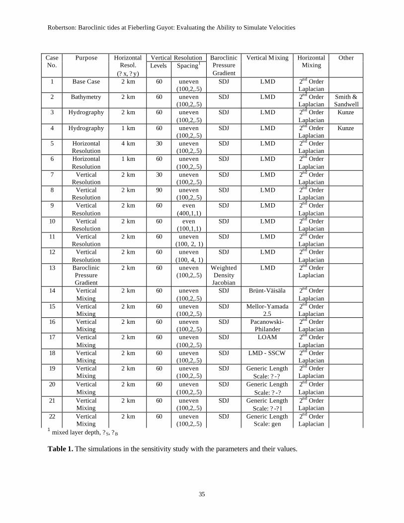
Table 1. List of simulations in the sensitivity study with the parameters and their values.

Table 2. The rms differences for the major axes of the tidal ellipses for each constituent from

the simulations.

Table 3. The rms differences in the minor axes of the tidal ellipses and inclinations for each

constituent from the simulations.


35

1 mixed layer depth, ?S, ?B Table 1. The simulations in the sensitivity study with the parameters and their values.

Vertical Resolution Case No.

Purpose Horizontal Resol.

(? x, ? y) Levels Spacing1

Baroclinic Pressure Gradient

Vertical M ixing Horizontal Mixing

Other

1 Base Case 2 km 60 uneven (100,2,.5)

SDJ LMD 2nd Order Laplacian

2 Bathymetry 2 km 60 uneven (100,2,.5)


Smith & Sandwell

3 Hydrography 2 km 60 uneven (100,2,.5)


Kunze

4 Hydrography 1 km 60 uneven (100,2,.5)


Kunze

5 Horizontal Resolution

4 km 30 uneven (100,2,.5)


6 Horizontal Resolution

1 km 60 uneven (100,2,.5)


7 Vertical Resolution

2 km 30 uneven (100,2,.5)



2 km 90 uneven (100,2,.5)



2 km 60 even (400,1,1)



2 km 60 even (100,1,1)



2 km 60 uneven (100, 2, 1)



2 km 60 uneven (100, 4, 1)


13 Baroclinic Pressure Gradient

2 km 60 uneven (100,2,.5)

Weighted Density Jacobian

LMD 2nd Order Laplacian

14 Vertical Mixing

2 km 60 uneven (100,2,.5)

SDJ Brünt-Väisäla 2nd Order Laplacian

15 Vertical Mixing

2 km 60 uneven (100,2,.5)

SDJ Mellor-Yamada 2.5

2nd Order Laplacian

16 Vertical Mixing

2 km 60 uneven (100,2,.5)

SDJ Pacanowski-Philander

2nd Order Laplacian

17 Vertical Mixing

2 km 60 uneven (100,2,.5)

SDJ LOAM 2nd Order Laplacian

18 Vertical Mixing

2 km 60 uneven (100,2,.5)

SDJ LMD - SSCW 2nd Order Laplacian

19 Vertical Mixing

2 km 60 uneven (100,2,.5)

SDJ Generic Length Scale: ? -?

2nd Order Laplacian

20 Vertical Mixing

2 km 60 uneven (100,2,.5)

SDJ Generic Length Scale: ? -?

2nd Order Laplacian

21 Vertical Mixing

2 km 60 uneven (100,2,.5)

SDJ Generic Length Scale: ? -? l

2nd Order Laplacian

22 Vertical Mixing

2 km 60 uneven (100,2,.5)

SDJ Generic Length Scale: gen

2nd Order Laplacian


36

Parameter Investigated M2 (cm s -1)

S2 (cm s -1)

K1 (cm s -1)

O1 (cm s -1)

Normalized Sum

Base Case

? x, ? y =2 km; 60 levels;

unevenly spaced; Splines Density Jacobian BPG; LMD Mixing

2.06

0.81

5.15

1.30

4.00

Bathymetry Smith & Sandwell 2.38 0.76 5.22 1.40 4.19 Kunze, 2 km 1.78 1.15 5.16 1.39 4.36 Hydrography

Kunze, 1 km 2.17 0.68 4.82 1.41 3.93

? x, ? y =4 km (30 levels)

2.65 0.93 5.70 1.64 4.81 Horizontal Resolution

? x, ? y =1 km (60 levels)

1.79 0.70 4.48 1.26 3.57

30 levels 2.15 0.91 5.17 1.63 4.43 90 levels 2.37 0.84 6.01 1.81 4.75 60 levels;

thermocline = 400m ?S=1, ?B=1

2.18 0.81 5.17 1.54 4.24

60 levels; thermocline = 100m

?S=1, ?B=1

2.12 0.94 5.13 1.42 4.28


?S=2, ?B=1

2.19 0.81 5.10 1.53 4.23

Vertical Resolution and Spacing


?S=4, ?B=1

2.13 0.88 4.87 1.48 4.21


Weighted Density Jacobian BPG

2.59 0.74 5.19 1.27 4.15

Brünt-Väisäla Frequency

2.25 0.90 5.11 1.46 4.32

Mellor-Yamada 2.5 2.16 1.00 5.08 1.44 4.39 Pacanowski-Philander 2.40 0.75 5.38 1.58 4.35

LOAM Mixing 2.39 0.69 5.40 1.61 4.30 LMD - SSCW 2.07 0.88 5.18 1.46 4.22

GLS Mixing: ? -? 2.10 0.79 5.19 1.41 4.09 GLS Mixing: ? -? 2.10 0.81 5.19 1.61 4.27 GLS Mixing: ? -? l 2.14 0.82 5.29 1.56 4.28

Vertical Mixing

GLS Mixing: gen 2.35 1.01 5.48 1.57 4.67

Table 2. The rms differences for the major axes of the tidal ellipses for each constituent from the simulations.


37

Minor Axis (cm s-1)

Inclination (o)

Parameter

Investigated

M2 S2 K1 O1 Normal- ized Sum

M2 S2 K1 O1 Normal- ized Sum

Base Case

? x, ? y =2 km; 60 levels;

unevenly spaced; Splines Density Jacobian BPG; LMD Mixing

1.71

0.52

3.32

0.65

4.00

34

45

50

41

4.00

Bathymetry Smith & Sandwell 1.31 0.51 3.49 0.81 4.05 34 50 41 46 4.05 Kunze, 2 km 1.48 0.56 3.23 0.60 3.82 37 51 42 33 3.85 Hydrography Kunze, 1 km 1.64 0.42 2.99 0.76 3.84 29 52 31 35 3.46 ? x, ? y =4 km

(30 levels) 1.83 0.45 3.74 0.89 4.43 30 47 48 52 4.13

Horizontal Resolution ? x, ? y =1 km

(60 levels) 1.53 0.45 2.76 0.78 3.80 34 54 40 36 3.86

30 levels 1.60 0.48 3.29 0.82 4.11 34 47 47 40 3.95 90 levels 1.78 0.52 3.61 0.82 4.39 36 48 44 48 4.19 60 levels;

mld1 = 400m ?S=1, ?B=1

1.71 0.49 3.31 0.76 4.11 34 49 43 46 4.07

60 levels; mld1 = 100m ?S=1, ?B=1

1.71 0.49 3.29 0.72 4.03 35 49 44 41 4.01

60 levels; mld1 = 100m ?S=2, ?B=1

1.79 0.47 3.32 0.74 4.07 38 47 43 50 4.25

Vertical Resolution and Spacing

60 levels; mld1 = 100m ?S=4, ?B=1

1.77 0.47 3.15 0.77 4.06 35 51 45 45 4.15


Weighted Density Jacobian BPG

1.67 0.46 3.58 0.67 3.96 35 54 27 38 3.67

Brünt-Väisäla Frequency Mixing

1.77 0.49 3.22 0.67 3.98 35 45 52 48 4.24

Mellor-Yamada 2.5 Level Closure

1.63 0.49 3.30 0.71 3.98 33 48 49 46 4.11

Pacanowski-Philander Mixing

1.73 0.47 3.33 0.77 4.10 32 50 36 37 3.68

LOAM Mixing 1.72 0.45 3.33 0.80 4.10 31 54 36 39 3.78 LMD -SSCW 1.68 0.50 3.26 0.68 3.96 36 48 47 46 4.17

GLS Mixing: ? -? 1.43 0.44 3.26 0.78 3.85 36 48 43 32 3.79 GLS Mixing: ? -? 1.58 0.46 3.25 0.84 4.06 37 48 37 38 3.83 GLS Mixing: ? -? l 1.64 0.46 3.37 0.79 4.05 34 55 36 41 3.93

Vertical Mixing

GLS Mixing: gen 1.94 0.50 3.52 0.93 4.57 35 46 44 43 4.01 Table 3. The rms differences in the minor axes of the tidal ellipses and inclinations for each constituent from the simulations.


38

-128.2 -127.8 -127.4

Longitude

32.0

32.2

32.4

32.6

32.8

Latit

ude

B2

B3

F2

F3F4,F5 C

R3

R2P

-128.2 -127.8 -127.4

Longitude

32.0

32.2

32.4

32.6

32.8

Latit

ude

a)b)

-400

-300

-200

-100

-50

50

100

200

300

(m)Figure 1. a) The bathymetry over the domain contoured from the data provided by Eriksen. The locations of the ten moorings are shown as crosses and labeled. b) The depth differences over the domain between the bathymetry from Eriksen and that of Smith and Sandwell.


39

Bottom

-4000

-2000

0D

ept

h (m

)

(cm s -1 )

-4000

-2000

0

Dep

th (m

)

-4000

-2000

0

Dep

th (m

)

32.0 32.2 32.4 32.6 32.8Latitude

-4000

-2000

0

Dep

th (

m)

127o 51.4'W

127o 41.0' W

127o 51.4'W

127o 41.0'W

a)

b)

c)

d)

01

23

45

6

7

8910

Figure 2. North-south transects of the major axes of the tidal ellipses for M2 at a) 127o 51.4’ W and b) 127o 41.0’ W and c) and d) for K1 at the same longitudes, respectively.


40

32 42.05 N128 2.70 W

32 28.64 N127 50.44 W

32 28.27 N127 48.57 W

32 26.56 N127 46.16 W

32 9.30 N128 0.49 W

32 25.75N127 50 W

32 24.61 N127 47.57 W

Major Axis (cm s-1 )

B2 F2 R2 C B3F3R34 8

0

1000

2000

Dep

th (m

)

4 8 120 4 8 4 8 12 4 8 12 4 8 12 4 8 12 4 8P

32 26.56 N127 46.70 W

4 8 12

0

1000

2000

Dep

th (

m)

8 160 4 8 8 16 8 16 4 8 12 4 8 12 4 8

a)

b) K1

M2

32 42.05 N128 2.70 W

32 28.64 N127 50.44 W

32 28.27 N127 48.57 W

32 26.56 N127 46.16 W

32 9.30 N128 0.49 W

32 25.75N127 50 W

32 24.61 N127 47.57 W

Major Axis (cm s-1 )

B2 F2 R2 C B3F3R3P

32 26.56 N127 46.70 W

4 8

0

1000

2000

Dep

th (m

)

4 80 4 8 4 8 4 8 4 8 4 8 4 8

c)Mean

Figure 3. Comparison of the major axes of the tidal ellipses from the model and observations for a) M2 and b) K1 and for the c) mean velocities. Model results are indicated by dots and observations by crosses with the observational uncertainty range indicates. The observation points and locations are given and the water depth indicated by hatching where appripriate.


41

-4000

-2000

0D

epth

(m)

12

34

56

78

910

Bottom32.0 32.2 32.4 32.6 32.8

Latitude

-4000

-2000

0

Dep

th (m

)

(cm s -1 )

127o 41.0' W

127o 41.40W

a)

b)

Figure 4. North-south transects of the major axes of the tidal ellipses for a) M2 and b) K1 at 127o 41.0’ W using the bathymetry of Smith and Sandwell.


42

Bottom

-4000

-2000

0D

ept

h (m

)

(cm s -1 )

-4000

-2000

0

Dep

th (m

)

-4000

-2000

0

Dep

th (m

)

32.0 32.2 32.4 32.6 32.8 33.0Latitude

-4000

-2000

0

Dep

th (

m)

a)

b)

c)

d)

01

23

45

6

7

8910

Figure 5. North-south transects of the major axes of the tidal ellipses for M2 at 127o 41.0’ W with grid cell resolutions of a) 4 km and b) 1 km and for K1 at the same resolutions c) and d) respectively.


43

Bottom

-4000

-2000

0D

epth

(m

)

(cm s -1 )

32.0 32.2 32.4 32.6 32.8

Latitude

-4000

-2000

0

Dep

th (

m)

127o 41.0'W

127o 41.0' W 1

2345

678910a)

b)

Figure 6. North-south transects of the major axes of the tidal ellipses at 127o 41.0’ W for a) M2 and b) K1 using a weighted density Jacobian for the baroclinic pressure gradient.


44

0

2

4

6

8

10

Bottom

(m s -1 )

-4000

-2000

0

Dep

th (m

)

-4000

-2000

0

De

pth

(m)

32.4 32.6 32.8

Latitude

-4000

-2000

0

Dep

th (m

)

d)a)

b)

c)

32.4 32.6 32.8

Latitude

e)

f)

LMD

MY

PP

GLS: k-kl

PP-LOAM

LMD-SSCW

h)

i)

j)

32.4 32.6 32.8

Latitude

GLS: gen

?

?GLS: k-

GLS: k-

-4000

-2000

0g)

BVF

Figure 7. A portion of a north-south transect of the major axes of the M2 tidal ellipses at 127o 41.0’ W for different vertical mixing parameterizations: a) Mellor-Yamada 2.5, b) Pacanowski-Philandar, c) Large-McWilliams-Doney, d) generic length scale version of the ?-?l parameterization, e) Pacanowski-Philandar with the LOAM modification, f) Large-McWilliams-Doney with the modifications, g) Brunt-Väisäla frequency, h) the generic length scale version of the ? -? parameterization, i) the generic length scale version of the ? -? parameterization, and j) the generic length scale version for a generic parameterization.


45

Figure 8. A portion of the north-south transect of the vertical momentum diffusivity averaged over one semidiurnal tidal cycle at 128o 41.0’ W for different vertical mixing parameterizations: a) observations from Kunze and Toole (1997) and Toole et al. (1997), b) a) Mellor-Yamada 2.5, b) Pacanowski-Philandar, c) Large-McWilliams-Doney, d) generic length scale version of the ?-? l parameterization, e) Pacanowski-Philandar with the LOAM modification, f) Large-McWilliams-Doney with the modifications, g) Brunt-Väisäla frequency, h) the generic length scale version of the ?-? parameterization, i) the generic length scale version of the ?-? parameterization, and j) the generic length scale version for a generic parameterization. In a), GW, 2004 refers to the values of Ganachaud and Wunsch (2004) and P, 1997 the observations of Polzin et al. (1997).

1E-005

1E-004

1E-003

Bottom-4000

-2000

0D

epth

(m

)(m2 s -1 )

-4000

-2000

0

Dep

th (

m)

-4000

-2000

0

De

pth

(m

)

32.4 32.6 32.8

Latitude

-4000

-2000

0

Dep

th (

m)

a)

e)b)

c)

d)

32.4 32.6 32.8

Latitude

f)

g)

LMD

MY

PP

GLS: k-kl

PP-LOAM

LMD-SSCW

i)

j)

k)

32.4 32.6 32.8

Latitude

GLS: gen

?

?GLS: k-

GLS: k-

-4000

-2000

0h)

Obs. BVF

GW

, 200

4P

, 19

97


46

Bottom32.0 32.2 32.4 32.6 32.8

Latitude

-4000

-2000

0

Dep

th (m

)

0.01

0.1

1

4

(m2 s-1)

a)

Figure 9. North-south transects of the gradient Richardson number calculated by the model at time= 28 days at 127o 41.0’ W.


47

Documents

Baroclinic Tides at Fieberling Guyot: Evaluating the Ability