Embed Size (px)
Citation preview
1. Introduction
1.1. Notation.
• P(Rn) := polynomials on Rn
• Hpm := harmonic polynomials of degree n, i.e. P (x) 3 ∆P = 0
• ∆ =∑∂2xi
• IQ := polynomials invariant under the orthogonal group O(Q)• Q(x) :=
∑x2i .
Problem. Describe the space HPm and IQ.
Lemma. IQ is formed of functions f(r2) : f ∈ C[x], where r2 =P∑i=1
x2i .
Proof. a) IQ is a homogeneous ring:
IQ = ⊕m≥0ImQ where m is the total degree.
b) The orbit of the line L1 = (x1, 0, . . . , 0) under SO(Q) is densein Rp.
f 7→ f |L1 = qf
is an injection into polynomial functions of one variable q satisfyingq(x) = q(−x). These are functions of the form q(x) = P (x2). Anysuch function is the restriction of an f ∈ IQ. Indeed, if (x1, . . . , xp) is
a point, and r =√x2
1 + · · ·+ x2p , f(x) := q(r2) is the candidate.
Structure ofHpm. We can construct such elements. First, if g ∈ O(Q),
f ∈ Hpm, then
(g · f)(x) = f(g−1 · x)
is also in Hpm. This is because in general,
∆(g · f)(x) = ∆(f)(g · x).
It is “easy” to find some functions in Hpm:
f(x) = (x1 ± ix2)m.
Question. To what extent are these “all” of Hpm.
Definition. Let G be a group, and V a finite dimensional complexspace. A representation is a group homomorphism
π : G→ GL(V ),
where GL(V ) is the group of invertible linear transformations of V .1
2
A representation is called irreducible, if any W ⊂ V invariantunder G is either (O), or V .
The formula (π(g)f)(x) = f(g−1x) defines a representation into thespace V of functions.
Theorem. HPm is irreducible.
So Hpm is generated by (x1 + ix2)m. But how do we write the answer
out systematically?We want to develop a geneal theory that deals with such questions.For GL(V ), with V a finite dimensional real or complex vector space,
• multiplication, µ : GL(V )×GL(V )→ GL(V ),• inverse, ι : GL(V )→ GL(V )
are differentiable, in fact even real or complex analytic. A Lie groupis a group G with a manifold structure such that multiplication andinverse are C∞. When V is a real n-dimensional vector space, we willwrite GL(n,R) ⊂ Mn(R) (' Rn2
= gl(n,R)) is an open subset. It isgiven by det 6= 0.
1.2. Linear Lie groups. An important class of Lie groups is givenby groups G ⊆ GL(n,R) which are closed subgroups in the inducedtopology.
An important feature is the exponential map: exp : gl(V ) →GL(V ).
exp(X) :=∑ X i
i!.
This is C∞, in fact analytic. Recall that exp(X + Y ) 6= expX · expY,and a local inverse near the identity Id is given by
log(X) =∑
(−1)i−1 (X − Id)i
ionly defined for X close to Id.
Definition. The Lie algebra g = L(G) of G is
g := X ∈ gl(n) | exp(tX) ∈ G ∀ t ∈ R.
More generally, a Lie algebra a, is a vector space with a skew linearmap
[ , ] : a× a→ a
satisfying
(a): [X, Y ] = −[Y,X],(b): [aX1 + bX2, Y ] = a[X1, Y ] + b[X2, Y ],(c): [X, [Y, Z]] + [Z, [X, Y ]] + [Y, [Z,X]] = 0.
3
Proposition. If G = O(Q), then
L(G) = X : X +t X = 0.
Proof. Recall the relations
(v, w) :=∑
viwi,
g ∈ O(Q)⇔ (gv, gw) = (v, w)⇔ tg · g = Id,
and
estX = t(esX).
Differentiate estX · esX = Id in s, and set s = 0:
tX +X = 0.
Conversely, assume tX + X = 0, same as tX = −X. Exponentiating,we get
etX = e−X = (eX)−1.
Other Examples.
Strictly upper triangular group.
N =
1 ∗
. . .0 1
n×n
, n =
0 ∗
. . .0 0
Heisenberg group.
Hn =
1 a1 · · · an−1 z
. . . 0 bn−1...b1
1
gn = p1 · · · pn−1, q1 · · · qn−1
[pi, pj] = [qi, qj] = 0, [pi, qj] = δijz
An interesting representation of the Heisenberg group:
V = C[x1, . . . , xn]
pi 7→ mxi
qi 7→ ∂xiz 7→ c · Id
4
Remark. In general, a representation of a Lie group gives rise to arepresentation of the corresponding Lie algebra by differentiation
π(X)v :=d
dt
∣∣∣t=0
π(etX)v.
Not all representations can be differentiated, e.g.
V = L2(R) (π(x)f)(y) := f(x+ y).
Theorem. g is a Lie algebra.
Proof. Assume etX ∈ G, esY ∈ G ∀ s, t ∈ R. We need to show thatet(X+Y ), et[X,Y ] ∈ G ∀t ∈ R. In general we can write
eX+Y =∞∑n=0
(X + Y )n
n!=∑n=0
1
n!
∑i1+i2+···+in=m,ij=0,1
X i1Y i2 · · ·X im−1Y im ,
and we can try to sort this out in terms of eX and eY . A better waymight be to consider
(etnX · e
tnY )n
=(I +
t
nX +
t2
2!n2X2 + · · ·
)(I +
t
nY +
t2
2!n2Y 2 + · · ·
)· · ·(I +
t
nY +
t2
2!n2Y 2 + · · ·
)= I + n · t
n(X + Y ) +
1
n(awful series).
The limit as n → ∞ is et(X+Y ). Since the original expression is in G,and G is closed, the limit is in G as well. This implies that X +Y ∈ g.
For [X, Y ] use(etnX · e
tnY · e−
tnX · e−
tnY)n2
= e[X,Y ]+ 1n
(awful series).
2. The differential of exp
We start with the easy observation that
d
dt
∣∣∣t=t0
etX = X · et0X = et0X ·X
The next theorem gives the formula for the differential of the exponen-tial map. If X ∈ g, a Lie algebra, denote by adX, the linear map
adX : g −→ g, adX(Y ) := [X, Y ].
5
This is linear, and satisfies
adX([Y, Z]) = [adX(Y ), Z] + [Y, adX(Z)],
ad[X, Y ] = adx adY − adY adX(= [adX, adY ]).
These relations come from the Jacobi identity. The first one meansthat adX is a derivation. The second one is interpreted as sayingthat the map
ad : g −→ gl(g)
is a Lie algebra homomorphism. In general, for a vector space V, wewrite gl(V ) for the Lie algebra of endomorphisms of V with the bracketstructure [A,B] := AB − BA. A Lie algebra homomorphism is alinear map satisfying:
F : g −→ h, F ([a, b]) = [F (a), F (b)].
If A ∈ End(V ), and
f(z) =∑
anzn
is a power series, define
f(A) :=∑
anAn,
provided the series∑|an|||A||n converges. In particular, for f(z) :=
1−ezz, the series
1− e−adX
adX:=∑n≥0
(−adX)n
(n+ 1)!
makes sense.
Theorem. Let λ : R→ g be any curve. Then
d
dteλ(t) = eλ(t) 1− e−adλ(t)
adλ(t)(λ′(t))
Proof. The following relations hold:
• adX = LX −RX , and LX , RX , adX commute,
• eλ(t) =∑∞
n=0(λ(t))n
n!,
6
where LX and RX are multiplication by X on the left and right respec-tively. Differentiate in t:
∞∑n=0
n−1∑k=0
λ(t)n−1−k · λ′(t) · λ(t)k
n!=∞∑n=0
1
n!
n−1∑k=0
(Ln−1−kλ(t) Rk
λ(t))(λ′(t))
=∞∑n=0
1
n!
Lnλ(t) −Rnλ(t)
Lλ(t) −Rλ(t)
(λ(t)) =eLλ(t) − eRλ(t)
adλ(t)(λ′(t))
= eλ(t) · 1− e−adλ(t)
adλ(t)(λ′(t)).
In particular, the differential at 0 of exp is the identity. So exp is alocal isomorphism from a neighborhood of 0 ∈ g to a neighborhood ofId ∈ G. So for X, Y small, there is Z(X, Y ) such that
eX · eY = eZ(X,Y ).
Of courseZ(X, Y ) = log(EX · eY ),
where
logA =∞∑n=1
(−1)n−1
n(A− I)n
is only defined for ‖A− I‖ < 1.But in fact Z(X, Y ) is a series in X, Y which is defined for all X, Y .
Question. What is this series?
Theorem (Campbell-Baker-Hausdorff). Let ψ(Z) := z log zz−1
. Then
log(eX · eY ) = X +
∫ 1
0
ψ(eadX · etadY )(Y )dt.
Proof. Define Γ(t) so that γ(0) = X, and
eΓ(t) = eX · etY .Then
eadΓ(t) = eadX · etadY
because in general,
eadZ(W ) = eLZ · e−RZ = LeZ ·Re−Z (W ) = eZ ·W · e−Z .Then by the previous result,
d
dteΓ(t) = eΓ(t)ϕ(−adΓ(t))(Γ′)(t)).
7
On the other hand, this is also
eX · etY · Y = eΓ(t) · Y
So
ϕ(−adΓ(t))(Γ′(t)) = Y.
Now
ψ(z) · ϕ(− log z) =z log z
z − 1· e− log z − 1
− log z=
z
z − 1·
1z− 1
−1= 1.
So
Γ′(t) = ψ(eadΓ(t))(Y ).
Integrating, we get the formula in the statement.
Corollary.
eX · eY = eX+Y+ 12
[X,Y ]+···
eX · eY · e−X = eY+[X,Y ]+···
eX · eY · e−X · e−Y = e[X,Y ]+···
These relations were used to prove that a closed linear group has aLie algebra, in fact is a Lie group.
Remark. For a closed subgroup G of GL(n), the exponential mapgives coordinates
exp : U∼−→ V
This makes G into a manifold.To define the Lie algebra of a linear group, we don’t even need G
closed. Define g as the set
X ∈ gl(n) | there exists a C1 path λX(t) ∈ G with λ′X(0) = X,λX(0) = I.
Then g is a Lie algebra, because we compute
d
dt
∣∣∣t=0eλX(t) · eλY (t) = X + Y,
d
dt
∣∣∣t=0eλX(at) = aX
d
dt
∣∣∣t=0eλX(t) · eλY (t) · e−λX(t) · e−λY (t) = [X, Y ].
Moreover,
X ∈ g⇒ etX ∈ G for all t ∈ R (moderately difficult) .
For X ∈ gl(n), we construct a vector field on G = GL(n)
H(g) := gX.
8
This is viewed as a tangent vector to G at g. An integral curve is acurve whose tangent vector is X at all points. In other words,
γ : (a, b)→ G
dγ
dt= X (γ(t)) = γ(t)X
If we specify γ(x0) = g0, this has a unique solution, which extends toall of R
γ(t) = g0 exp tX.
2.1. Suppose we have a continuous group homomorphism
Ψ : G→ GL(m)
G ⊂ GL(n), a closed linear group. If X ∈ g, we can look at ψ(exp tX).This is a continuous homomorphism
Γ : R→ GL(m).
Indeed, exp(t1 + t2)X = exp t1X · exp t2X, and Ψ is a group homo-morphism. But any such homomorphism is in fact C∞, and there is Ysuch that
ψ(exp tX) = etY .
For |t| < ε, a small ε > 0, look at
γ : R→ gl(m)
γ(t) = log Γ(t)
γ(t1 + t2) = γ(t1) + γ(t2) for |t1|, |t1| <ε
2.
This extends to an additive continuous map
γ : R→ gl(m)
Let Y := γ(1).So we get a Lie algebra map
dψ : g→ gl(m).
it also follows that if the map Ψ is continuous, it is C∞.Conversely, if you have a Lie algebra map
ψ : g→ GL(m),
defineΨ(g) = ψ(log g).
This is defined for g in a small open set c ∈ V . The CBH formulaimplies that in fact
Ψ(g1g2) = Ψ(g1) ·Ψ(g2)
9
provided g1, g2, g1 · g2 ∈ V .
Example. G = S1, L(G) = Rψ(t) = tX.
Then Ψ(eiθ) = eirθ is not necessarily defined for all θ, because
e2πi = 1⇒ e2rπi = Id.
Example. (e2πiθ, e2πiτθ) with τ irrational is dense in T 2 = S1 × S1.This is a Lie group.
Example. The Lie algebra so(3) is the subalgebra of gl(3) of skewsymmetric matrices. A basis is given by
e2 =
0 0 10 0 0−1 0 0
, e1 =
0 1 0−1 0 00 0 0
, e3 =
0 0 00 0 −10 1 0
.
It acts on functions in Hm by the formulas
f ∈ Hm (X · f)(x1, x2) :=d
dt
∣∣∣t=0f(etX ·
(x1
x2
)).
This is a Lie algebra representation, i.e.
[X, Y ] · f = X · (Y · f)− Y · (X · f), f ∈ Hm ⇒ X · f ∈ Hm
and a lot easier to deal with, than the group action that it comes fromby differentiation, (g · f)(x) := f(g · x). The bracket relations are
[e1, e2] = e3, [e2, e3] = e1, [e3, e1] = e2.
We can also compute
e1 · (x1 + ix2)m = im(x1 + ix2)m
[(e2 + ie3) · (x1 + ix2)m] = i(m− 1)[(x1 + ix2)m−1].
Of course there is an analogue of this action for all dimensions. Thesimplest one is for p = 2 :
Hm2 = a(x1 + ix2)m + b(x1 − ix2)m,
and the group acting is
SO(2) =
(cosθ sin θ− sin θ cos θ
).
It acts by e±imθ on the two vectors (x1± ix2)m. O(2) is the product ofSO(2) with another element, with action(
cosθ − sin θ+ sin θ cos θ
)(x1
x2
)=
(cos θx1 − sin θx2
+ sin θx1 + cos θx2
).
10
It takes (x1 + ix2)m to (x1 − ix2)m
3. Representations of R as a Lie algebra.
Since R is generated by 1, as a vector space, the assignment 1 7→M,some n × n matrix, determines the representation, t 7→ tM. Up tosimilarity of M , these are the same representation (π, V ) and (ρ,W )are called equivalent, if there is an invertible linear map A : V → W ,such that
ρ(g) A = A π(g) ∀ g ∈ GM1 A = A M2 ⇒M2 = A−1M1A.
So Equivalence classes of representations of R ↔ Jordan canonicalforms of matrices.
For Rn, a representation is determined by n commuting matrices.
Lie algebras of dimension 2. let e1, e2 be a basis of the Lie algebra.Then up to equivalence, there are two possible structures:
• [e1, e2] = 0,• [e1, e2] = e2.
Continuous representations of S1. A continuous representation πof S1 is an assignment eiθ 7→ M(θ), where M(θ) is an n× n invertiblematrix depending continuously on θ, and such that
M(θ1+θ2) = M(θ−1)·M(θ2), M(−θ) = M(θ)−1, M(2iπ) = Id.
For small θ, we can consider
dπ(θ) := R(θ) = logM(θ).
Then R(θ) extends uniquely to a representation of (R,+). Let X :=R(1). Then π(θ) = eiθX . This describes all the continuous represnta-tions of S1; They are the exponentials of the representations of R, butwith matrices that satisfy e2iπX = Id. There is an inner product on Cn
so that all operators are unitary. Indeed, take any inner product 〈 , 〉on Cn
(v, w) =1
2π
∫ 2π
0
〈M(θ)v,M(θ)v〉dθ
By differentiating, we find that the matrix X is skew hermitian. Letv1, . . . , vn be a basis of eigenvectors of X. Then each subspace Cvi isstabilized by π(S1), and forms an irreducible representation. The fullspace decomposes into a direct sum
Cn = ⊕Cviof π(S1) invariant subspaces. S1.
11
Lie algebras of dimension 3. (over C) . One of the main examplesis sl(2,C) :
sl(2,C) = e, h, f [h, e] = 2e(0 10 0
),
(1 00 −1
),
(0 01 0
)[h, f ] = 2f
[e, f ] = h
This is the Lie algebra of the Lie subgroup SL(2,C), two by two ma-trices of determinant 1.
Exercise 1. Classify all Lie algebras of dimension 3.
You should find the abelian one, sl(2) and the Heisenberg algebra,p, q, z, p, q] = z, [p, z] = [q, z] = 0. A example of a representation isp 7→ mx, q 7→ ∂x, z 7→ 1. Can also think of the Heisenberg algebra as0 a c
0 0 b0 0 0
.
Representations of sl(3). Recall V = xαyβa+b=N , the space ofhomogemneous polynomials of degree N is two variables has dimensionN + 1. We can define a representation of Sl(3) by the formula(
a bc d
)· xαyβ = (ax+ by)α · (cx+ dy)β
We differentiate to get a representation of the Lie algebra. A basis ofsl(3) is given by
e =
(0 10 0
)h =
(1 00 −1
)f =
(0 01 0
).
Then, (1 t0 1
)xαyβ = (x+ ty)αyβ
so e · xαyβ = αxα−1yβ+1. Furthermore,(1 0t 1
)· xαyβ = xα(tx+ y)β
so f · xαyβ = βxα+1yβ−1. Finally,(et 00 et
)xαyβ = eαt · e−βtxαyβ
so h · xαyβ. Thus xN is “killed” by e, and has h-eigenvalue N .
12
Consider SU(2), the subgroup of Sl(3,C) of unitary matrices. ItsLie algebra is generated by
e1 =
(i/2 00 −i/2
),
e2 =
(0 1/2−1/2 0
),
e3 =
(0 i/2i/2 0
).
These basis vectors satisfy
[e1, e2] = e3, [e2, e3] = e1, [e3, e1] = e2.
On the other hand, we saw that so(3) also has a basis satisfying theserelations, so su(2) ∼= so(3). The representations constructed earlier forSL(2), give rise to representations of so(3). We would like to identifythe representations of So(3) onHm with the ones constructed above. Sofar we know that we get representations of SU(2) this way by restrictingthe representations of SL(2,C).
We know that there is a Lie algebra map
ψ : su(2)→ so(3) ⊆ R3.
We would like to exponentiate this map to the group. This is possible,identify R3 with skew hermitian matrices. The inner product is
〈A,B〉 := tr(AB∗)
Then
SU(2) =
(α β−β α
): |α|2 + |β|2 = 1
.
it is also the group of 2 × 2 matrices satisfying g · g∗ = Id. Define amap
Ψ : SU(2) −→ Aut(R2), Ψ(g) · A = gAg−1.
Then
〈g · A, g ·B〉 = tr(gAg−1 · g∗−1B∗g∗) = tr(AB∗),
so Ψ maps SU(2) to O(3). In fact it is SO(3); because SU(2) isconnected. We can compute the kernel of Ψ, it is ±Id. In fact weget an exact sequence
1→ ±Id → SU(2)→ SO(3)→ 1.
So representations of SU(2), trivial on−I drop down to SO(3), and anyirreducible representation of SO(3) comes from an irreducible repres-ntation of SU(2), trivial on ±Id.
13
Irreducible finite dimensional representations of sl(2,C)
First, we analyze the relation to representations of su(2). Complexifythe algebra. Then
[2ie1, e2 + ie3] = 2i(e3 − ie2) = 2(e2 + ie3)
[2ie1, e2 − ie3] = 2i(e3 + ie2) = −2(e2 − ie3)
[e2 − ie3, e2 + ie3] = ie1 + ie1 = 2ie1
Seth = 2ie1, e = e2 + ie3, f = e2 − ie3
π(h) must have an eigenvector v
π(h)v = λv
Thenπ(h)π(e)v = π(e)π(h)v + π([h, e])v = (λ+ 2)v.
So assume also that π(e)v = 0 called highest weight vector.vλ, vλ−2 = π(f)v, π(f)2v, . . . , π(f)nv = vλ−2n linearly independent.
This spans V , because (π, V ) is assumed irreducible. Let N be suchthat π(f)vλ−2N = 0.
(λ− 2N)vλ−2N = (π(e)π(f)−π(f)π(e))vλ−2N = −π(f)(cλ−2Nvλ−2N+2)
π(e)π(f)n = π(f)π(e)π(f)n−1 + π(h)π(f)n−1
= π(f)2π(e)π(f)n−2 + π(f)π(h)π(f)n−2 + π(h)π(f)n−1
= π(f)nπ(e) +n−1∑k=0
π(f)kπ(h)π(f)n−k−1
applied to vλ, and n = N ,
(λ) + (λ− 2) + · · ·+ (λ− 2N + 2) = Nλ−N · (N − 1) = N(λ−N + 1).
λ− 2N = −Nλ+N2 −N(N + 1) · λ = N2 +N = N · (N + 1)⇒ λ = N
So each N ∈ N has an irreducible module (πN , VN) attached to it.
Realization: VN = xayb : a+ b = N has dimension N + 1.Action of SL(2,C) is(
a bc d
)· x = ax+ cy
(a bc d
)· xrys =(
a bc d
)· y = bx+ dy (ax+ cy)r · (bx+ dy)s
14
Differentiation gives
e1 =1
2ih = − i
2h, e2 =
e+ f
2, e3 =
1
2i(e− f).
But note that
e2πih =
(1 00 1
)e2πe1 =
1 0 00 1 00 0 1
eht · vΛ = eΛtvΛ ete1 · vΛ = e−
ti2hvΛ = e−
tΛ2 vΛ
For e−2πΛ
2 to be 1, need Λ ∈ 2N.So only the odd dimensional representations occur.
4. Review of Manifolds
4.1. Basic Notions.
• M , a locally Euclidean space of dimension d. This means aHausdorff topological space where each point has a neighbor-hood ' U, an open set of Rd
ϕ : U → V ⊆ Rd
• Differentiable structure of class Ck (k = ∞, ω), is a clooectionof charts (Uα, ϕα) : α ∈ A
(a)⋃Uα = M
(b) ϕα ϕ−1β is Ck
(c) Uα is maximal.• Uαα∈A a cover by open sets is called locally finite if for anym ∈ M there exists V open such that V ∩ Uα 6= φ for finitelymany α ∈ A only. M is called paracompact if any open coverhas a locally finite open subcover.
A topological space which is locally compact, Hausdorff andsecond countable, is paracompact.• A partition of unity is a collection ϕi : i ∈ I where the φi areC∞ functions satisfying,
(a) supp ϕi : i ∈ I is locally finite(b)
∑ϕi(p) = 1 ∀ p ∈M , ϕi ≥ 0.
We only consider manifolds which are locally compact, Hausdorff, sec-ond countable.
Theorem. Any cover Uαα∈A of M has a countable partition of unityϕi : i ∈ I subordinate to Uα with suppϕi compact.
(subordinate means that for any i, suppϕi ⊂ Uα for some α.)
15
4.2. Germs. Fix m ∈ M . Two functions f, g ∈ C∞(M) define thesame germ atm, if there is a neighborhood V ofm, such that f |V = g|V .
We use the following notation.
: Fm the algebra of germs at m. Then f ∈ Fm has a well definedvalue f(m).
: Fm := germs which vanish at m.
There is a descending sequence of ideals
Fm ⊃ F2m ⊃ F3
m · · · .
Definition. A tangent vector at m is a derivation
D : Fm → R, D(f · g) = f(m) ·Dg +Df · g(m),
D(af + bg) = aD(f) + bD(g)
We denote by
Mm := the linear space of tangent vectors. ThenMm ' (Fm/F2M)∗
has dimension d.
Tangent vectors come from curves via differentiation. Let
λ : I →M, where I = (−c, c) λ(0) = m.
The tangent vector at m associated to λ is
vλ(f) =d
dt
∣∣∣t=0f(λ(t)).
If
Ψ : M → N is a C∞ map,
then it induces a map
Ψm,∗ : Mm → Nm, Ψm,∗(v)(f) := v(f Ψ).
There is a commutative diagram
TMΨ∗−−−→ TN
πM
y πN
yM
Ψ−−−→ N
16
4.3. Tangent Bundle.
T (M) =∐m∈M
Mm, T (M)π→M, π(vm) = m.
T (M) has the following manifold structure. If (U,ϕ) is a chart, ϕ =(ϕ1, . . . , ϕd),
ϕ : π−1(U) → V × Rd
(r, vr) 7→ (ϕ(r), ϕ∗(vr)(f))
where ϕ∗(vr)(f) =d
dt
∣∣∣t=0
(f ϕ)(λvr(t)))
Vector Fields: Recall π : T (M) → M. Any C∞-map X : U →π−1(U) such that π X = idU is called a vector field.
If f ∈ C∞(U), then we can define X (f)(m) := (Xmf)(m).In coordinates,
X =∑
ai∂
∂xi,
where ai are C∞. It satisfies
X (f · g) = X (f) · g + f · X (g).
A curve σ : I →M is called an integral curve for X , if
·σ(t) = X (σ(t))
σ(0) = m is called the initial condition.
Notation.·σ = dσ
dt
Theorem. Let X be a C∞ vector field. For any m ∈ M there exista(m) < 0 < b(m) and a C∞ curve
γm : (a(m), b(m))→M
such that
γm(0) = m,·γ(t) = X(γ(t)).
The integral curve is unique in the sense that if
µ : (c, d)→M µ(0) = m,
is another curve, then a(m) ≤ c < 0 < d ≤ b(m) and µ(t) = γm(t).
17
We can define a transformation
Xt : Dt →M
Xt(m) = γm(t)
where Dt = m ∈M : t ∈ (a(m), b(m)). The theorem implies that forfixed t, Dt is open. Then
Xt is smooth,Xt Xs = Xt+s,
Definition. X is called complete, if Dt = M ∀t.
5. Lie groups
A Lie group is a C∞ manifold G, with a group structure such that
m : G×G→ G m(x, y) = x · y,
i : G→ G i(x) = x−1
are C∞. Fix a g ∈ G. Define
Lg : G→ G Lg(x) = gx,
Rg : G→ G Rg(x) = xg,
Ad(g) : G→ G Ad(g) = Lg Rg−1 = Rg−1 Lg,and
g := TeG.
Recall that
(Lg)∗,x : TxG→ TgxG.
Definition. A vector field X : G→ TG is called left invariant, if
(Lg)∗,x(X (x)) = X (gx))
Similarly for right invariant vector fields. The vector space of left in-variant vector fields will be denoted L(G).
Proposition. L(G) ' g as a vector space.
Proof. Let X ∈ g. Define X (g) := (Lg)∗,e(X). This is a left invariant,C∞-vector field. The assignment X ∈ g 7→ X gives the isomorphism.
Proposition. L(G) is a Lie algebra under the usual bracket.
18
Proof. This is mostly left as an exercise. It is better to look at vectorfields as acting on functions
[X, Y ](f) := X(Y (f))− Y (X(f)).
If Ψ : M → N , (ψ = Lg, M = N = G) is an isomorphism, andY ∈ V ec(N), define Ψ∗(Y )(m) = Ψ−1
∗,ψ(m)(Y (Ψ(m)):
TMΨ−1∗←−−− TN
Ψ∗(Y )
x Y
xM
Ψ−−−→ N
On functions,
Ψ∗(Y )(f)(m) = Y (f Ψ−1)(ψ(m))
If X ∈ V ec(M), define
Ψ∗(X )(n) = Ψ∗,ψ−1(n)(X (ψ−1(n)))
Ψ∗(X )(f)(n) = X (f Ψ)(ψ−1(n))
Remark. If Φ : M → N is a diffeomorphism, Φ∗ is usually calledAdjΦ,
Adj(Φ)(X ) = Φ−1∗ X Φ.
Of course Φ∗ is just Adj(Φ∗).Then
Ψ∗([X1,X2]) = [Ψ∗X1,Ψ∗X2]
Ψ∗([Y1,Y2]) = [Ψ∗Y1,Ψ∗Y2].
Exercise 2. Complete the details of the proof.
A vector field X is left invariant, iff
(Lg)∗(X ) = X (Lg(x) = gx).
Indeed,
[(Lg)∗X ](x) := (Lg)∗,g−1xX (g−1x) = X (g · g−1x) = X (x).
19
Integral curves. If X ∈ g, let X is the left invariant vector field inL(G), satisfying X (e) = X. Write γX(t) (= γX(t, e)) for the integralcurve of X with initial condition γX(0) = e. So
·γX(t) = X (γ(t)) = (Lγ(t))∗,e(X).
Fix a g, and consider µ(t) := gγX(t) = Lg(γX(t)). Then·µ(t) = (Lg)∗,γ(t)(
·γX(t)) == (Lg)∗,γ(t)(X (γ(t)) = X (gγ(t)).
Thus µ(t) is the integral curve for X with initial condition µ(0) = g.We can thus extend γX(t) defined for t ∈ (−ε, ε) as follows. Note thatγX(ε/2)γX(t) is defined for t ∈ (−ε, ε), and
γX(t) =
γX(t) (−ε, ε)γX( ε
2)γX(t− ε
2) t ∈ ( ε
2, 3ε
2)
γX(− ε2)γX(t+ ε
2) t ∈ (−3ε
2,− ε
2)
is an integral curve with initial condition γX(0) = e. The domain ofdefinition is (−3ε
2, 3ε
2). Continuing this way, we conclude that any left
invariant vector field is complete.We define expG(X) := γX(1).
Remark. In general,
γ(g, t0 + t) = γ(γ(g, t0), t)
exp(t1X + t2X) = exp t1X exp t2X.
Lie brackets. Let x ∈M , X ,Y ∈ V ec(M) with flows µ and ν. Let
Γx(t, τ) = ν(µ(ν(x,−t), τ), t).
Proposition.
[X ,Y ](x) =∂2
∂t∂τ
∣∣∣(0,0)
Γx(t, τ).
Proof. Compute∂2
∂t∂τ
∣∣∣(0,0)
f(Γx(t, τ))
for a C∞ function f. Note that t occurs in two places, so differntiatingin t first, we get:
∂
∂τ
∣∣∣τ=0Y(f)(µ(x, τ)) +
∂
∂τ
∣∣∣τ=0
( ∂∂t
∣∣∣t=0f(µ(ν(x,−t), τ)
)= X (Y(f))(x) +
∂
∂t
∣∣∣t=0
∂
∂τ
∣∣∣τ=0
f(µ(ν(x,−t)), τ)
= X (Y(f)) +∂
∂t
∣∣∣t=0Y(f)(ν(x,−t)) = X (Y(f))− Y(X (f)).
20
For a Lie group, µX(g, τ) = g exp τX, ν(h, t) = h exp tY . So the curveis Γx(t, τ) = x exp−tY exp τX exp tY . Recall also that
·µ(t) = (Lg)∗,γ(t)(
·γX(t)) = (Lg)∗,γ(t)((Lγ(t))∗,e(X))
= (Lgγ(t))∗,e(X) = X (µ(t)).
In other words, µ(t) is the integral curve with initial condition µ(0) =g.
We define a map
expG : g→ G, expGX := γX(1).
The map will be abbreviated exp when it is clear what the group is.
Proposition. exp is C∞.
Proof. Let V = TeG. Define
U : G× V → T (G× V ) = T (G)× V
U(g, v) := ((Lg)∗,e(V ), 0).
Let (Ω1,Ω2) be its flow; it depends C∞ on the initial condition (g0, v0).Then Ω2(t) is constant, equal to the initial condition v0.
·Ω1(t) = (LΩ1(g,v,t))∗,e · Ω2 = (LΩ1(g,v,t))∗,e(v) = g exp tv
because Ω2(t) ≡ v.Setting t = 1, the basic theorem implies (g, v) 7→ g exp v is C∞ in
the initial condition (g, v).
Corollary. exp∗,0 = Id, so exp is a local diffeomorphism, in otherwords there are neighborhoods 0 ⊂ U, and e ⊂ V, such that
exp : U∼→ V.
Let now F : G→ G′ be a local homomorphism.
Proposition. The following diagram commutes:
gdF−−−→ g′
expG
y expG′
yG
F−−−→ G′
21
Proof. Let µ(t) := F (exp tX)
d
dt
∣∣∣t=t0
F (exp tX) =d
dx
∣∣∣t=0F (exp(t0X + tX))
=d
dt
∣∣∣t=0F (exp t0X) · F (exp tX)
= (LF (exp t0X))∗,e dFe(X).
Corollary. Two locally isomorphic Lie groups have the same Lie alge-bra.
Theorem. The Lie algebra of a commutative Lie group is commuta-tive.
Proof.
ν(µ(ν(x,−t), τ), t) = µ(ν(x,−t), τ) · exp tY
= ν(x,−t) · exp τX · exp tY
= x · exp−tY · exp τX · exp tY
= x exp τX.
Corollary. If [X, Y ] = 0, then
expX · expY = exp(X + Y ).
In particular, expX and expY commute.
Proof. Let α(t) = µ(ν(x, t), t). This is also
α(t) = exp tY · exp tX,
and satisfiesα(1) = expY · expX.
But
α′(t) = (µt)∗(Y(ν(x, t)) + X (α(t))) = (µt)∗(Y(µ−t(α(t)))) + X (α(t))
= (Y + X )(α(t)).
Again, we have used the fact that t appears in two places; so whenyou differntiate, you get a sum where you set one t constant, anddifferentiate the other one).
We have used the following lemma:
Lemma. Suppose X ↔ µ, Y ↔ ν. Then
d
dt[Adj(νt)(X )] = [Adj(νt)X ,Y ].
22
Proof. First note that
ν(x, t) = ν(ν(x, s), t− s).So Adjνt = Adjν−t0 · Adjνt0 . Also, Adjνt(Y) = Y . Thus,
Adj(νt)(X ) = Adjνt−t0(Adjνt0(X )),
and[Adj(νt)(X ),Y ] = Adjνt[X ,Y ].
Thus it is enough to prove
d
dt
∣∣∣t=0
[Adj(νt)(X )] = [X ,Y ].
But Adj(νt)(X ) = (νt)∗ X ν−t on a function f , is given by
d
dτ
∣∣∣τ=0
f(ν(µ(x,−t), τ), t)).
The previous formula gives the result.
Alternate Version.d
dt
∣∣∣t=t0
d
dτ
∣∣∣τ=0
exp tXexpτY exp−tX
= (Lexp t0X)∗ · (Rexp−t0X)∗∂2
∂t∂τ
∣∣∣t=τ=0
(exp tX exp τY exp−tX)
= (L...) R...([X ,Y ](e)) = 0.
Sod
dτ
∣∣∣τ=0
(exp tX · exp τY · exp−tX) = Y.
But the curve µ(t) = g exp tXg−1 is the integral curve for Ad(g)X 3Ad(g)(X)1 = (Lg)∗ (Rg−1)∗(X).
Soexp tX exp τY exp−tX = exp τY.
Corollary. Assume G connected. Then G abelian ⇔ g abelian.
Theorem. Let F : G → G′ be a local, continuous homomorphism.Then F is C∞.
Proof. This is true for G = R. Choose a basis X1, . . . , Xn for g. Then
t 7→ F (exp tXi)
is a continuous homomorphism from (R,+) to G′. So it is C∞. To beprecise, there is Yi ∈ g′, so that F (expG tXi) = expG′ tYi. Recall thatexpG′ is a local diffeomorphism near e′. Write logG′ for the local inverse.
23
We can form t 7→ logG′ F (expG(tXi)). This extends to a homomorphismfrom (R,+) to g′,+, so is of the form t 7→ Yi.
For (t1, . . . , tn) sufficiently small, define
(t1, . . . , tn) 7→ exp t1X1 · · · exp tnXn.
This is a local diffeomorphism at 0. Then
F (exp t1X1 · · · exp tnXn) = exp t1Y1 · · · exp tnYn
which is C∞.
Corollary. If G and G′ are locally isomorphic, then g ' g′ Conversely,if G1 ∼ G2 topologically, then ⇒ G1 ∼ G2 as Lie groups. A topologicalgroup has at most one Lie structure.
Adjoint Representation.
Ag : G→ G Ag(x) := gxg−1
d(Ag) := Ad(g) : L(G)→ L(G)
satisfies
Ad(g)([X, Y ]) = [Adg(X), Adg(Y )]
and also Ad(g1 · g2) = Ad(g1) · Ad(g2). So
Ad : G→ GL(g)
is a representation. Define ad : g→ gl(g) to be d(Ad). Then there is acommutative diagram
gAd(g)−−−→ g
expG
y expG
yG
Ag−−−→ GSo
Ag(expG ξ) = expGAd(g)ξ
g · expG ξg−1 = expG(Ad(g)ξ).
Theorem. adξ(η) = [ξ, η].
Proof.
ad(ξ) = d(Ad)(ξ) = Ad∗,e(ξ) =d
dt
∣∣∣t=0Ad(exp tξ)
24
applied to η, we get
ad(ξ)(η) =d
ddt
∣∣∣t=0Ad(expG tξ)(η)
=d
dτ
∣∣∣τ=0
d
dt
∣∣∣t=0
exp tξ exp τη exp−tξ = [ξ, η].
We also have another diagram
gad−−−→ gl(g)
expG
y expGL
yG
Ad−−−→ GL(g)So
Ad(expGX) = eadX ,
andexpG(eadX(Y )) = expGX · expG Y · expG(−X).
Indeed,Ad(expGX)(Y ) = eadX(Y )
and
expG(eadX(Y )) = expG(Ad(expGX)(Y )) = AexpGX(expG Y )
= expGX · expG Y · expG(−X).
Differential of exp. Define γg(s) = g exp(X+sY )·exp(−X),·γg(0) =
g. Then·γg(0) = (Lg)∗(Rexp−X)∗,expX exp∗,X(Y ).
WriteΨ(X)(Y )(g) :=
·γg(0).
Proposition.
Ψ(X)(Y )(e) =eadX − IadX
(Y ).
Proof. Let α(t) := Ψ(tX)(tY )(e). Then show·α(t) = Y + adX(α(t)).
On the other hand, consider
ρ(t) =eadtX − IadtX
(tY ).
Then ρ(0) = 0, and
dρ
dt=∞∑n=0
tn+1 (adX)n
(n+ 1)!(Y ) =
∞∑n=0
tn(adX)n
n!Y = Y + adX(ρ(t)).
25
This implies the assertion, since α(0) = 0, and using uniqueness ofsolutions to D.E.
So we compute·α :
d
dt
∣∣∣t=τ
d
ds
∣∣∣s=0
exp(tX + stY ) exp(−tX)
=∂2
∂t∂s
∣∣∣s=0,t=τ
(exp(tX + stY ) exp(−τX) + exp(τX + τsY ) exp−tx)
=∂2
∂σ∂s
∣∣∣s=σ=0
(exp(σX + σsY ) exp(τX + τsY ) exp(−τX))
+− d
ds
∣∣∣s=0
X(exp(τX + τsY ) exp(−τX))
=∂2
∂σ∂s
∣∣∣σ=s=0
exp(σX) exp(τX + τsY ) exp(−τX)
+∂2
∂σ∂sexp(σX + σsY )− d
ds
∣∣∣s=0
X(exp(τX + τsY ) · exp(−τX))
= Y (e) +·γexp(σ(X))(0)(τX, τY )− d
ds
∣∣∣s=0
X(γe(s))
Recall
exp∗,X(Y ) = (RexpX)∗eadX − IadX
(Y )
Corollary. The local structure of a Lie group is determined by its Liealgebra structure.
Proof.
log(expX · expY ) = X +
∫ 1
0
ϕ(eadX · eadtY )(Y )dt
where ϕ(z) = z log zz−1
.Same proof as for GL(N). This is the Baker-Campbell-Haussdorff
formula.
Corollary. For any Lie algebra homomorphism
F : g→ g′,
there is a local group homomorphism
F : G→ G′.
Proof. Define
F (expGX) := expG′ f(X).
26
Since expG is a local diffeomorphism near 0, F is well defined. Thefact that F (g1g2) = F (g1)F (g2), follows from the formula in the proofof the above corollary.
5.1. Brief Review of Homotopy.
Definition. Let X be arcwise connected. We say X is simply con-nected, if every closed curve is contractible.
Definition. Two curves
γ1 : [0, 1]→ X γ2 : [0, 1]→ X
satisfying
γ1(0) = γ2(0) = x1, γ1(1) = γ2(1) = x2
are homotopic if there exists a continuous map H,
H : [0, 1]× [0, 1]→ X
H(t, 0) = γ1(t), H(t, 1) = γ2(t)
H(0, s) = x1, H(1, s) = x2.
Contractible means γ(t) ∼ γ0(t) ≡ x0
Theorem. Let G be simply connected, and F : U ⊆ G → G′ a localhomomorphism. Then F extends uniquely to a homomorphism.
Proof. Let e ∈ V0 be a neighborhood such that V0·V0 ⊂ U , and F (gh) =F (g) · f(h), g, h ∈ V0. Let V ⊂ V0 be such that V · V −1 ⊂ V0.
Given a curve γ : [a, b]→ G, partition
[a, b] a = a0 < a1 · · · < an = b
so that if t1, t2 ∈ [ai, ai+1], then γ(t1) ·γ(t2)−1 ∈ V0. Set γi = γ(ai−1)−1 ·γ(ai), and K(γ) =
∏F (γi).
Exercise 3. Show that
• K(γ) is independent of the partition.• K(γ) only depends on the homotopy class of γ.• K(g0γ) = K(γ).• K(γ1 ∗ γ2) = K(γ1) ·K(γ2).• If Imγ ⊂ V , K(γ) = F (γ(a))−1 · F (γ(b)).• If γ ≡ g0, then K(γ) = e.
Recall multiplication in π1(X). If γ1 : [0, 1] → X, γ2 : [0, 1] → Xand γ1(1) = γ2(0), then
γ1 ∗ γ2(s) =
γ1(2s) 0 ≤ s ≤ 1
2
γ2(2s− 1) 12≤ s ≤ 1.
27
If g ∈ G, choose γ : [0, 1]→ G, γ(0) = e, γ(1) = g,
F (g) := K(γ).
The proof follows from these properties.
Corollary. Locally isomorphic simply connected groups are isomor-phic.
5.2. Review of Covering Spaces. Recall γ1∗γ2 and γ−(t) = γ(1−t).Define
π1(X, x0) := Homotopy classes of closed curves with endpoints x0π1(X, x0) is a group with ∗ and −. If f : X → Y , can define
f# : π1(X, x0)→ π1(Y, f(x0)).
This is independent of x0, if X is arcwise connected.
Definition. p : Y → X is called a covering of X if for each x, there isa neighborhood U such that p−1(U) is a disjoint union of neighborhoodsso that p is an isomorphism with U on each of them.
Proposition. Let γ be a curve, and y0 ∈ p−1(γ(0)). There is a uniquelift γ : [0, 1]→ Y , p γ = γ, γ(0) = y0.
Proposition. Let γ1, γ2 be homotopic (with fixed endpoints), and γ1 ,γ2 be lifts with γ1(0) = γ2(0) = y0. Then γi are homotopic.
Proposition. p : Y → X with Y arcwise connected. Then π1(X, x0)acts transistively on p−1(x0).
Theorem. p : Y → X a covering, Y arcwise connected, X simplyconnected. Then p is an isomorphism.
Theorem. Suppose X is locally simply connected, arcwise connected.There is a 1-1 correspondencebetween normal subgroups H ⊆ π1(X, x0)and covering maps p : Y → X.
5.3. Coverings of Lie Groups. We now apply the general theory toA connected Lie group G.
Theorem. π1(G, e) is abelian, and ∗ is induced by
(γ · δ)(t) := γ(t) · δ(t).
Proof.
h(t, x) =
γ(2t− ts)δ(st) 0 ≤ t ≤ 1
2
γ(1− s(1− t)) · δ(2t− 1 + s(1− t)) 12≤ t ≤ 1
28
g(t, s) =
γ(st)δ(2t− 2s) 0 ≤ t ≤ 1
2
γ(2t− 1 + s(1− t)) · δ(1− s(1− t)) 12≤ t ≤ 1
Theorem. Let G be a connected Lie group. ∃! simply connected Lie
group G which is a covering group,
p : G→ G, and ker p = π1(G)
is a central subgroup.
Proof. G exists and is unique as a topological space. A realization isas homotopy classes γ of curves satisfying γ(0) = e, with p(γ) :=
γ(1), [γ] · [δ] = [γ · δ]. This is a group homomorphism, and G is a Liegroup. Let now [γ0] ∈ ker p, i.e., γ0(0) = γ0(1) = e. Look at
[γ]→ [γ] · [γ0] · [γ]−1.
This maps G to G, with image in ker p. Because it is continuous, it isconstant. So the kernel is a central subgroup.
Spin groups
An important set of examples of covering groups are the Spin groups,which are the simply connected cover groups of the orthogonal groups.Versions of these groups over fields other than R and C figure promi-nently in number theory. We will mostly deal with the even orthogonalgroups over C. The main reference is the book by Fulton and Harris.
5.4. Clifford Algebra.
• V a vector space/C• Q a quadratic form
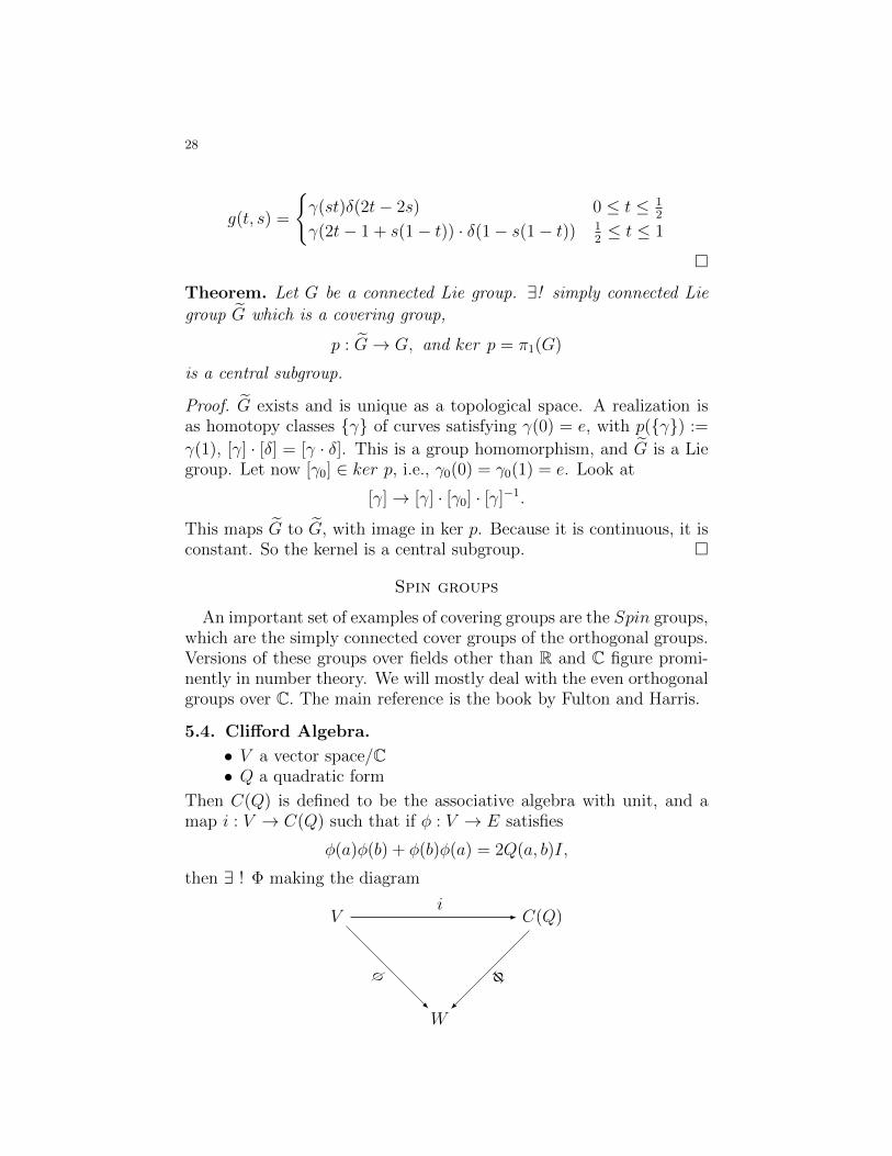
Then C(Q) is defined to be the associative algebra with unit, and amap i : V → C(Q) such that if φ : V → E satisfies
φ(a)φ(b) + φ(b)φ(a) = 2Q(a, b)I,
then ∃ ! Φ making the diagram
Vi
- C(Q)
W
Φφ
-
29
commutative.
Construction: C(Q) := T (V )/a⊗ b+ b⊗ a−Q(a, b)• Q ≡ 0 gives Λ∗∨• a⊗ b− b⊗ a gives S ′(V )• a⊗ b− b⊗a− [a, b] gives the universal enveloping algebra U(g).
Basis of C(Q): Pick e1, . . . , en, an ordered basis of V . Then
ei1 · ei2 · · · eik1≤i1<i2<···<ik≤n
is a basis of C(Q). Furthermore,
C(Q) = C(Q)ev ⊕ C(Q)odd,
the even and the odd parts.
Assume Q nondegenerate. C(Q) is also a Lie algebra.
5.5. Relation to so(Q). Recall that
so(Q) := X ∈ End(V ) : Q(Xv,w) +Q(v,Xw) = 0.First, observe that so(Q) ' Λ2V . The map is a ∧ b 7→ φa∧b, given by
ϕa∧b(v) = 2Q(b, v)a− 2Q(a, v)b.
Exercise 4. Show that [ϕa∧b, ϕc∧d] corresponds to
= 2Q(b, c)a ∧ d− 2Q(b, d)a ∧ c− 2Q(a, d)c ∧ b+ 2Q(a, c)b ∧ d.
Next define
ψ(a ∧ b) =1
2(a · b− b · a) ∈ C(Q).
Thenψ ϕ−1 : so(Q) → C(Q)ev,
and this is a Lie algebra homomorphism.
From here on, we assum that dimW is even. Then V = W ⊕W ′
so that Q|W ≡ 0, Q|W ′ ≡ 0. Thus W , W ′ are in duality via Q. Letv1 · · · vn, and w1 · · ·wn be dual bases. Then
(5.5.1) so(Q)↔[vi ∧ wj vi ∧ vjwi ∧ wj vi ∧ wj.
]This corresponds to the fact that in this basis,(5.5.2)
Q←→[0 II 0
]so(Q)←→
[A BC −tA
], A ∈ gl(n), B, C skew symmetric.
30
Theorem. C(Q) ' End(Λ∗W ).
Proof. To get a map
C(Q)→ E = End(Λ∗W ),
need a map ` from V to E, satisfying some conditions. We need
(5.5.3)
` : W → E, `′ : W ′ → E,
satisfying
`(w)2 = `′(w′)2 = 0, `(w) · `′(w′) + `′(w′)`(w) = 2Q(w,w′).
Define
(5.5.4)`(w)ξ := w ∧ ξ
`′(w′)(ξ1 ∧ · · · ∧ ξr) :=∑
(−1)i−1Q(w′, ξi)ξ1 ∧ · · · ξi · · · ∧ ξr.
Exercise 5. Complete the argument.
The spin representations. There is decomposition
Λ∗W = ΛevW ⊕ ΛoddW,
and this is respected by the action of C(Q)ev.
C(Q)ev = End(ΛevW )⊕ End(ΛoddW ).
Since so(Q) maps to C(Q)ev, we get two representations of so(Q), S±.
Proposition. S± are irreducible as so(Q) representations.
Proof. This follows from the fact that so(Q) generates C(Q)ev.
But we can also see the finer structure. Define
τ(w1 · · ·wr) = wr · · ·w1,
α(w1 · · ·wr) = (−1)rw1 · · ·wr.Let ∗ = α τ . Then (xy)∗ = y∗x∗, α(xy) = α(x)α(y). Define
Spin(Q) = x ∈ C(Q)ex : xx∗ = 1 and x · V · x∗ ⊂ V .There is a map
ρ : Spin(Q)→ SO(Q),
ρ(x) · v = x · v · x∗.Define
Pin(Q) = x ∈ C(Q) : x · x∗ = 1 x · v · x∗ ⊂ V ,ρ : Pin(Q)→ 0(Q) ρ(x)v = α(x) · v · x∗.
Then
31
• Spin(Q) is connected,• ρ is surjective,• ρ has kernel ±I.
The representations S± do not exponentiate to SO(V ). Let e1, . . . , en, f1, . . . , fnbe a basis of V
3 Q(ei, ej) = Q(fi, fj) = 0, Q(ei, fj) = δij.
so(Q) =X =
[A BC −tA
]: B + tB = 0, C + tC = 0
J =
[0 II 0
]XJ + J tX = 0.
So a basis of so(Q) is given by Eij − Ej+n,i+n, i = j ≤ n,
Eij − Ej−n,i 1 ≤ i ≤ n < j ≤ 2n
Eij − Ej,i−n 1 ≤ j ≤ n < i ≤ 2n.
The matchup is
Zij = Eij − Ej+n,i+n ↔ ϕ 12ei∧fj .
Then e2π√−1Zi,i = Id, but 1
2ei ∧ fi 7→ 1
2(eifi − 1). Then
1
2(eifi − 1)(eI) =
1 if i ∈ I0 otherwise
and e2π√−1 1
2(eifi−1) hasd eigenvalues −1.
5.6. Fundamental groups. Recall that
SO(n)/SO(n− 1) ' Sn−1.
If n > 2, π1(Sn−1)(= π2(Sn−1)) = 0. The long exact sequence of ofhomotopy groups implies that
π1(SO(n)) ' · · · ' π1(SO(3)) ' Z2.
On the other hand,
π1(SO(n,C)) ' π1(SO(n)).
This is because any matrix decomposes uniquely as M = U · S withU unitary, S hermitian. This is called the polar decomposition. But iftM ·M = Id, then S = (tM ·M)1/2 satisfies this as well, and thereforeso does U . In other words, if M ∈ SO(n,C), then U, S ∈ SO(m,C)as well. In fact there is a C∞-diffeomorphism
SO(n)× S ∈ so(n,C) hermitian → SO(n,C)
(k,X) 7→ k expX.
32
The second part involving exp is contractible.
5.7. Symplectic Group. Q nondegenerate skew form on V , dimVeven. Then there are similar results as in the orthogonal case’:
Q(a, b) = −Q(b, a)
sp(Q) = X ∈ End(V ) | Q(Xa, b) +Q(a,Xb) = 0Sp(Q) = x ∈ Aut(V ) | Q(xa, xb) = Q(a, b)
sp(Q) ' S2(V ) (sp(Q) −→[wiw
′j wiw
′j
w′iw′j wiw
′j
])
(a · b)(ξ) = Q(a, ξ)b+Q(b, ξ)a.
Exercise 6. Sp(Q) is simply connected.
This follows from the fact that the compact groups Sp(m) := Sp(m,C)∩U(2m) satisfy
(5.7.1) Sp(m)/Sp(m− 1) ∼= S4n−1.
The details are quite hard without further background material on thestructure of compact groups.
5.8. Unitary Groups. SU(n) is simply connected for n ≥ 2. Thisfollows from
SU(n)/SU(n− 1) ' S2n−1
For n = 2 get S3.
6. Covering groups of compact groups
Assume G is a covering group of a compact group G, i.e.
1→ Z → G→ G→ 1
with Z central and discrete.
Theorem. Assume that g = [g, g]. Then G is compact.
Proof. (I) There is a compact set K ⊂ G such that
K · Z = G.
For each g ∈ G, pick Ug ⊆ G open, with U g compact, and p : Ug →p(Ug). Extract a finite subcover of G. Then
K =⋃
U gi
satisfies the requirements.
33
we may as well assume K = K−1.
(II) There are finitely many z1, . . . , zn ∈ Z 3 Kz1, . . . , Kzn coverK ·K−1.
This follows from⋃z∈Z Kz ⊃ K ·K−1.
(III) Let Z1 ⊂ Z be the subgroup generated by the zi. Let
p1 : G→ G/Z1
Then p1(K) is a subgroup. This is because any k1 · k2 = k · z1 for some
k ∈ K, z1 ∈ Z1. Since it contains an open set, p1(K) = G/Z1, so G/Z1
is compact.To complete the proof, it is enough to show thatZ1 is finitep1(Z) is finite (why?!)The second assertion is clear.Z1 is finitely generated, abelian. If it is infinite, there is a nontrivial
ϕ : Z1 → C, ϕ(z1z2) = ϕ(z1) + ϕ(z2)
(Z1 ' Zk ⊕ (Z/pk11 )⊕ · · · ⊕ (Z/pkrZ) with k > 0).
Suppose ϕ extends to a Φ : G→ CΦ(g1g2) = Φ(g1) + Φ(g2).
Then dΦ : g→ C is Lie homomorphism, and so dΦ([x, y]) = 0, becauseC is an abelian Lie algebra. Since g = [g, g], then dΦ ≡ 0, so Φ istrivial. This contradicts Φ|Z1 = ϕ 6= 0.
(IV) Recall K = K−1 compact ⊆ K1 ⊂ K1. Let f0 ≥ 0 be such that
f0(g) =
1 g ∈ K0 g /∈ K1
Writeσ0(g) =
∑z∈Z1
f0(gz−1).
Then 0 < σ0(g) <∞ for any g ∈ G. This is because on the one handthere is at least one z 3 gz ∈ K, and on the other hand, gZ1 ∩K1 isdiscrete and closed, so finite.
Let
f(g) :=f0(g)
σ0(g).
Then ∑z∈Z1
f(gz) = 1.
34
Defineψ0(g) :=
∑z∈Z1
f(gz−1)ϕ(z) +∑z∈Z1
f(z)ϕ(z).
Thenψ0(z0) = ϕ(z0) z ∈ Z1
ψ0(z0) =∑z∈Z1
f(z0z−1)ϕ(z) +
∑f(z)ϕ(z)
=∑
f(u)(ϕ(u−1) + ϕ(z0)) +∑
f(z)ϕ(z) = ϕ(z0)
ψ0(gz0) =∑
f(gz0z−1)ϕ(z) +
∑f(z)ϕ(z)
=∑
f(gu−1)ϕ(z−10 u) +
∑f(z)ϕ(z)
ψ0(g) + ψ0(z0).
SetΨ1(g, h) := ψ0(gh)− ψ0(h).
ThenΨ1(g, hz) = ψ0(ghz)− ψ0(hz) = Ψ1(g, h),
so it drops down to G× G/Z1; call this Ψ2(g, γ).Let
Φ(g) =
∫G/Z1
Ψ2(g, γ)dγ.
Then
Φ(z) =
∫G/Z1
Ψ2(z, γ)dγ
andΨ1(z, γ) = ψ0(zγ)− ψ0(γ) = ψ(z).
If we normalize so that∫G/Z1
dγ = 1, Φ(z) = ϕ(z). Furthermore
Φ(g1g2) =
∫G/Z1
ψ2(g1g2, γ)dγ
ψ2(g1g2, γ) = ψ0(g1g2γ)− ψ0(γ)
=∑z∈Z1
f(g1g2γz−1)ϕ(z)−
∑z∈Z1
f(γz)ϕ(z)
= ψ2(g1; g2γ) + ψ2(g2; γ).
35
Integrating, and using the invariance of dγ, we get
Φ(g1g2) = Φ(g1) + Φ(g2).
6.1. Remark. s : SO(n) → Aut(S), S spin representation comesfrom 〈v, w〉 =
∑viwi, C(V ), this time V = Rn.
We can define an operator on functions F : V → S
F = (f1, · · · , fdimS) dimS = 2n
D =∑
∂xiS(xi).
Then
D2 =∑i,j
∂xi∂xjs(ei)s(ej)
=∑i≤j
∂xi∂xj [s(ei)s(ej) + s(ej)s(ei)]
= 2∑
∂2xi
(acting on each coordinate).
7. Lie Subgroups
7.1. Frobenius Theorem. We follow F. Warner’s book.
Definition. A d-dimensional distribution on a manifold M , is a choiceof d-dimensional subspace
m 7→ D(m) ⊆ TmM
which is smooth in m.A submanifold (N,ψ) is called integral for D, if ψ∗(TnN) = D(ψ(n))∀n ∈ N .D is called involutive if X (m) , Y(m) ∈ D(m) ∀m ⇒ [X ,Y ](m) ∈D(m) as well.
C∞ means that for each m0 ∈ M , there exists Vm0 ⊆ M , a neigh-borhood, and d linearly independent vector fields X1, . . . , Xd so thatspanX1(m), . . . , Xd(m) = D(m), ∀m ∈ Vm0 .
Theorem. (Frobenius) D involutive ⇔ through each point passes aunique submanifold integral for D. Fix an m ∈ M . There exists acoordinate system ((x1, . . . , xn), U) so that xi = ci, i > d from integralsubmanifolds.
36
7.2. Application to Lie Groups.
Theorem. Let h ⊆ g be a Lie subalgebra, G a connected Lie groupwith Lie algebra g. There exists a unique Lie subgroup H ⊆ G with Liealgebra h.
Proof. Construct a distribution H by
H(g) = (Lg)∗,e(h).
We can choose a basis X1, . . . , Xd of h, and then X1, . . . ,Xd arelinearly independent at every g, span H(g), and
[Xi,Xj](g) = (Lg)∗,e[Xi, Xj].
Then X (g) ∈ H(g) for any g ∈ G if and only if
H(g) =d∑i=1
ai(g)Xi(g) ∀ g ∈ G.
This implies that H is involutive because(7.2.1)[∑
aiXi,∑
bjXj]
=∑i,j
(aibj[Xi, Xj] + aiXi(bj)Xj − bjXj(ai)Xi
)Let (ϕ,He) be the maximal connected integral submanifold through
e ∈ G. If h ∈ He, then Lh−1(He) is also an integral manifold passingthrough e. Thus Lh−1He = He, so He is a group.
Write He for H. We also need to check that
α : H ×H → H α(x, y) = x−1y
is C∞. Write τ for the map τ(x, y) = x−1y on G. Then τ is C∞. Wehave β = τ (ϕ× ϕ), and
H ×H ϕ×ϕ→ G×G τ→ G,
which is C∞. So α is in a commuting diagram
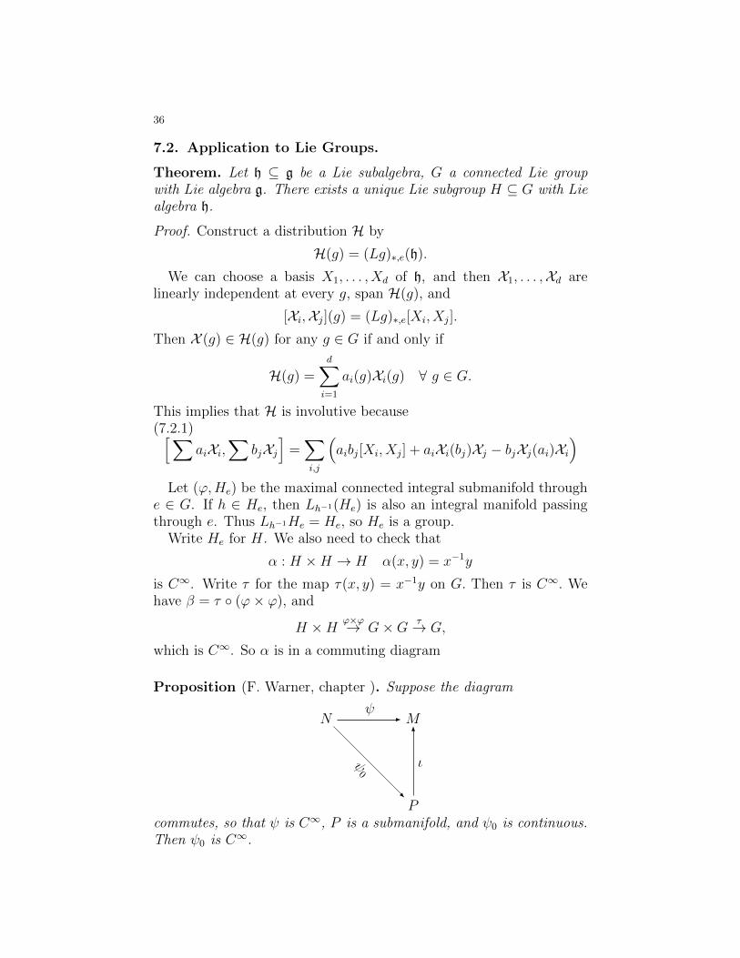
Proposition (F. Warner, chapter ). Suppose the diagram
Nψ- M
P
ι
6
ψ0
-
commutes, so that ψ is C∞, P is a submanifold, and ψ0 is continuous.Then ψ0 is C∞.
37
Proposition. Suppose, that the diagram above commutes, ψ0 arbi-trary, but P is involutive for a distribution D. Then ψ0 is continuous(and therefore C∞).
Theorem. Let (H,ϕ) be a Lie subgroup of G. Then ϕ is an imbedding⇔ H is closed.
Proof. Assume ϕ(H) is closed. To show the claim, it is enough to showthat there is an open set V ⊆ H such that ϕ|V is a homeomorphism ofV into ϕ(H) with the relative topology. Using translations by h ∈ H,the claim follows for all h ∈ H.
Let (U, τ) be coordinates at e, such that ϕ(H) ∩ U is a countableunion of slices. Let e ∈ C ⊂ U be closed, and S be given by
S : τ1 = 0, . . . , τd = 0
ϕ(H) ∩ U : τd+1 = cd+1, . . . , τn = cn
Then τ(ϕ(H) ∩ S) is non empty, closed, countable. Thus it has anisolated slice S0. Conversely, let σi ∈ H with σi → σ ∈ G. Choose acoordinate neighborhood (U, τ) near e so that ϕ(H)∩U is a single sliceS. Choose V ⊆ W ⊆ U such that V −1 · V ⊆ W ⊆ U . Then σn ∈ σVfor n ≥ N . Then σ−1
N σn ∈ W , so σ−1N σ ∈ W . But σ−1
N σn ∈ S ∩W , soσ−1N σ ∈ S, i.e., σ ∈ H.
Theorem. Let H ⊂ G be a closed topological subgroup of a Lie groupG. Then H is a Lie group.
Proof. Let
h := X ∈ g : exp tX ∈ H ∀t ∈ R.Then h is a Lie subalgebra of g. The proof is the same as for subgroupsof GL(n), (
exp1
nX · exp
1
nY)n→ exp(X + Y )(
exp1
nX · exp
1
nY · exp− 1
nX · exp− 1
n
)n2
→ exp[X, Y ].
Let H0 be the subgroup corresponding to H. Then H0 ⊆ H. Wewant to show H0 = H. Let hn ∈ H, hn /∈ H0 be such that hn → e.Write g = h⊕ s, and write
hn = expXn · expYn Xn ∈ h, Yn ∈ s.
Then Xn → 0, Yn → 0.
38
May as well use hn = expYn, Yn ∈ s. Write Yn = anZn, with an > 0,an → 0, Zn → Z0 6= 0. For any t > 0, let [ t
an] = j(n) ∈ Z. Then
an · j(n) = t+ xn, and
xn → 0(xn = an
( t
an−[ tan
])).
Then
exp anZn ∈ H, (exp anZn)j(n) ∈ H
limn→∞
(exp anZn)j(n) = exp tZ0.
Since H is closed, Z0 ∈ h ∩ S, a contradiction.
7.3. Homogeneous Manifolds. Let H ⊂ G be a closed Lie sub-group. Let G/H be the coset space, π : G→ G/H.
Theorem. There exists a unique C∞ structure on G/H such that(a) π is C∞
(b) there exist local smooth sections of G/H to G, i.e., if σH ∈ G/H,∃ σH ∈ W ⊂ G/H open, and τ : W → G, C∞ so that π τ = id.G/H called homogeneous space.
Proof. See F. Warner, section 3.58. The idea is as follows. As in theprevious proof, write g = s ⊕ h. Let 0 ∈ U1 × U2 ⊂ h × S be smallenough so that
(X1, X2) 7→ expX1 · expX2
is a diffeomorphism onto an open neighborhood e ∈ V ⊆ G.Because H is closed, we can arrange it so that
expX1 · h1 = expX1 · h2
if and only if X1 = X ′1. Thus
τ : U1 → G/H τ(X1) = expX1 ·H
can be used as coordinates.
Remark. The structure is such that the map G×G/H → G/H givenby left multiplication is C∞.
39
Examples.
• SO(n)/SO(n−1) ' Sn−1, SU(n)/SU(n−1) ' S2n−1, Sp(n)(Sp(n−1) ' S4n−1.• Flag Varieties A generalized flag is a collection
(0) ⊂ V1 ⊂ V2 ⊂ · · · ⊂ Vk = V
with fixed dimensions dimV1 = i1 < dimV2 = i2 < · · · <dimVk = dimV. The set of flags is denoted F(i1, i2, . . . , ik) ThenGL(V ) acts on F(i1, . . . , ik) in the obvious way. The action istransitive, if α1, α2 ∈ F(i1, . . . , ik) there exists g ∈ GL(V ) suchthat g · α1 = α2.
Fix a basis e1 · · · en, and a flag
e1, . . . , ei1 ⊂ ei1+1, . . . , ei1+i2 ⊂ . . . ⊂ ei1+···+ik−1+1, . . . , en.The stabilizer is the block upper triangular group P formed ofmatrices of the form
(7.3.1)
GL(i1) ∗ . . .
0 GL(i2 − i1) . . .0 0 . . .. . . . . . . . .0 0 GL(ik − ik−1)
This is a closed subgroup, called a parabolic subgroup. Then
G/P ' F(i1, . . . , ik).
If you use an orthonormal basis, one can also prove that
F ∼= U(n)/[U(i1)× U(i2 − i1)× · · · × U(ik − ik−1)].
8. Review of Lie Algebras
Definition. The center of g is
Z(g) = X ∈ g : [X, Y ] = 0 ∀Y ∈ g.An ideal of g is a Lie subalgebra J ⊆ g, such that [g,J ] ⊆ J .
Proposition. Suppose G a connected Lie group, and J ⊆ g an ideal.Then the (connected) group I ⊆ G corresponding to I is a normalsubgroup.
Proof. Let X ∈ g. Then
(LexpX)∗,e (Rexp−X)∗,expX(J ) = eadX(J ) = J .Then since exp is a local diffeomorphism near 0,
(8.0.2) Ad(g)(J ) = J ,
40
for g ∈ G near e. Since any neighborhood of e generates G, it followsthat Ad(g)(J ) = J for all g ∈ G. Now I is the submanifold so that
TiI = (Li)∗,e(J ), ∀i ∈ I.Then gIg−1 has tangent space at gxg−1 equal to
(Lg)∗xg−1(Rg−1)∗,x(Lx)∗,e(J ) = (Lgxg−1)∗,eAd(g)(J ) = (Lgxg−1)∗,e(J ).
So they are both integral manifolds for J passing through e. ThusgIg−1 = I.
Proposition. Let I ⊂ G be a normal subgroup. Then J := L(I) is anideal.
Proof. (Lexp tX)∗,exp−tX (Rexp−tX)∗,e(J ) = J , and this can be writtenas
etadX(J ) = J .Differentiating, we get
(8.0.3) adX(J ) ⊂ J .
Definition. A Lie algebra is called simple, if it has no nontrivial ideals,and dim g > 1.
Lower Central Series.
D1g = [g, g], . . . ,Dkg = [g,Dk−1g].
Derived Series. D1g = [g, g], Dkg = [Dk−1g,Dk−1g].Nilpotent means Dkg = 0 for some kSolvable means Dkg = 0 for some k.
Definition. Lie groups are called nilpotent/solvable, if their Lie alge-bras are so.
9. Nilpotent and solvable algebras
References:Humphreys, I.2 and I.3 , Jacobson, II.3, II.4, II.6 , Helgason III.1,
III.2.
A subspace I ⊆ g is called an ideal if [g, I] ⊆ I.
Definition. The derived series is defined inductively by
(1) D1g = [g, g],(2) Di+1g = [Dig,Dig].
41
Lemma. Dig is an ideal.
Proof. We do an induction on i. D1g is an ideal by the Jacobi identity.Similarly let X ∈ Di, Y ∈ Di and Z ∈ g. Then
ad[X, Y ] = adX adY − adY adX
so[[X, Y ], Z] = [X, [Y, Z]]− [Y, [X,Z]]
Then apply the induction hypothesis.
Definition. A Lie algebra is called solvable if Dng = 0 for some n > 0.
The lower central series is defined as
(1) C1g = [g, g],(2) Ci+1g = [g, Cig].
Definition. An algebra is called nilpotent if Cng = 0 for some n > 0.
Since Cng ⊇ Dng nilpotent implies solvable.
Proposition.
(1) Every subalgebra and every quotient of a solvable algebra is solv-able.
(2) If I ⊆ g is a solvable ideal such that g/I is solvable, then g issolvable.
(3) The sum of two solvable ideals is solvable.
Proof. (1) If h ⊆ g then Dih ⊆ Dig. If 0 → I → gπ−→ h → 0, then
π−1Dih ⊆ Dig.(2) If I and h are solvable, π(Dnh) = 0 for some n. So Dng ⊆ I. But
then Dn+mg ⊆ DmI = 0 for large m.(3) follows from (1) and (2): 0 → I1 → I1 + I2 → I2/I1 ∩ I2 → 0,
I1 + I2/I1 ' I2/I1 ∩ I2.
Examples: b =
∗ ∗. . .
0 ∗
, n =
0 ∗. . .
0 0
are solvable and
nilpotent respectively. sl(n) on the other hand is neither.
Proposition. The sum of two nilpotent ideals is nilpotent.
Proof. Let X1 ∈ I1 and X2 ∈ I2. Then
(9.0.4) (adX1 + adX2)m(Y ) =∑
adXi1 · · · adXim(Y )
with ij = 1 or 2. If mi are such that CmiIi = (0), then (9.0.4) iscontained in one of CmiIi so it is zero. Then apply Engel’s theorem
42
which is proved later. You can also prove directly that Cm(I1+I2) = (0)but this is more tedious.
Let S ⊂ g be a solvable ideal of maximal dimension. If I is anyother solvable ideal, S + I is solvable. Since S ⊆ S + I the maximalityimplies S = S +I, or I ⊆ S. Thus S is unique; it is called the solvableradical. If S = (0), we say g is semisimple. If g has no proper nonzeroideals and Dg 6= 0, we say g is simple.
Corollary. g contains a nilpotent ideal of maximal dimension N , calledthe nilradical.
Note that N ⊆ S.
Lemma.
(1) g/S is semisimple.(2) If g is simple, then g is semisimple.
Proof. (2) Let S ⊆ g be the radical. Either S = g or S = 0. If S = g,then DS = Dg 6⊆ g so DS = 0. But then Dg = 0 which contradictsthe definition of simple. Thus S = (0), i.e. g is semisimple.
(1) Let I ⊆ g/S be solvable. Its inverse image contains S andis solvable by proposition 9. Thus the inverse image is equal to S,i.e. I = (0).
Lemma. A finite dimensional Lie algebra g is solvable if and only ifevery nonzero ideal contains a subideal of codimension 1.
Proof. If g is solvable, Dg 6= g. Any linear subspace Dg ⊆ I ⊆ gis an ideal. Since g is solvable, D1g 6= g, we can find an ideal I ofcodimension 1. Conversely, since g contains an ideal of codimension 1,D1g 6= g. By induction Di+1 6= Di+1, and the claim follows from thefact that g is finite dimensional.
Note: If I1 is a subideal of I, i.e. [I, I1] ⊆ I1, this doesn’t mean it isan ideal of g.
9.1. Flags and Engel’s theorem.
Notes and talk prepared by Todd Kemp.
Proposition. If g/Z(g) is nilpotent, so is g.
Proof. There is an n such that gn ⊆ Z(g), since (g/Z(g))n = Z(g).Thus gn+1 = [ggn] ⊆ [gZ(g)] = 0.
Lemma. If g is nilpotent, adx is nilpotent for any x ∈ g.
43
Proof. Indeed, for n such that Cng = (0),
(9.1.1) [x1, [x2, [· · · [xny]] · · · ]]] = 0
for all xi, yi ∈ g. In other words, adx1adx2 · · · adxn(y) = 0, ∀ xi, yi ∈ g.Thus, letting xi = x ∀ i, (adx)n = 0, so adx a nilpotent endomorphism.
We say x is ad-nilpotent if adx is a nilpotent endomorphism. Thus,if g is nilpotent, then all x ∈ g are ad-nilpotent. The converse is Engel’stheorem.
Theorem. If x ∈ gl(V ) is a nilpotent endomorphism, then adx isnilpotent.
Proof. Define Lx(y) = xy, Rx(y) = yx. Then if xn = 0, Lnx(y) = xny =0, and Rn
x(y) = yxn = 0. Thus, Lx, Rx are nilpotent endomorphisms.Since g`(V ) is associative, Lx and Rx commute.
Let a, b be nilpotent in a ring R, and ab = ba. Then
(9.1.2) (a+ b)n =∑(
n
m
)an−mbm
So suppose ak = 0, b` = 0. Choose n > ` + k. Then, in the terman−mbm, if n − m < k, then m > n − k ≥ `. So bm = 0. Otherwisen−m ≥ k, so an−m = 0. Thus (a+ b)n = 0.
So, Lx−Rx is nilpotent. But adx = Lx−Rx, so adx is nilpotent.
Theorem. Let g be a subalgebra of g`(V ), V 6= 0 finite dimensional.If every element of g is nilpotent, then ∃ v ∈ V \0 with g · V = 0.
Proof. We do an induction on dim(g). In the case dim(g) = 1, this isjust the claim that a single nilpotent linear transformation always hasan eigenvector (with eigenvalue 0). This is standard linear algebra.
So let dim(g) > 1. Let h ⊂ g be a subalgebra. By lemma (9.1), anyadx is nilpotent, so acts on g as an algebra of nilpotent linear trans-formations. In particular h acts on g/h by nilpotent trasnformations.By induction, there is x ∈ g not in h such that
(9.1.3) [x, h] ⊂ h.
This means that the normalizer of h is strictly larger than h. Choose amaximal proper subalgebra h. For such an algebra,
(9.1.4) Ng(h) = g,
So h is an ideal of g and therefore g/h is an algebra.
44
We claim h is codimension 1. Indeed any subspace h ⊂ k ⊂ g isa subalgebra contradicting the maximality of h. Then we can find anelement z /∈ g so that
(9.1.5) g = h + Kz.
By the induction hypothesis, as dim h < dim g, there is 0 6= v ∈ V sothat h · v = 0.; In other words, W = v ∈ V ; h · v = 0 is nonzero. Buth is an ideal, so if x ∈ g, y ∈ h, [x, y] ∈ h. Thus
(9.1.6) (yx)w = xy · w − [xy]w = 0 · 0 = 0 ∀ w ∈ W.
So xW ⊆ W . In particular z ∈ g \ h maps W → W . It is nilpotent, sothere is 0 6= v ∈ W such that z · v = 0, The claim follows.
Theorem (Engel). If all elements of g are ad-nilpotent, then g is nilpo-tent.
Proof. We do an induction on the dimension of g. The claim is truefor dim g = 1. The assumptions imply that adg ⊆ g`(g) consists ofnilpotent endomorphisms. So there is 0 6= x ∈ g satisfying ady(x) = 0∀ y ∈ g, i.e. , [y, x] = 0 ∀ y ∈ g. Thus x ∈ Z(g) 6= 0 and so Z(g) 6= (0).
Thus g/Z(g) is clearly ad-nilpotent, and has smaller dimension. Bythe induction hypothesis, g/Z(g) is nilpotent. So by proposition 9.1, gis nilpotent.
Corollary. If g is nilpotent, then any nonzero ideal h has nontrivialintersection with Z(g). In particular, Z(g) 6= 0.
Proof. g acts via ad on h, so by theorem 9.1, there is 0 6= x ∈ h killedby g, i.e. , [g, x] = 0, so x ∈ h ∩ Z(g).
Definition. A flag in V is a chain (Vi) of subspaces
(9.1.7) 0 = V0 ⊆ V1 ⊆ · · · ⊆ Vn = V with dimVi = i.
We say x ∈ End(V ) stablizes (Vi) if x · Vi ⊆ Vi ∀i.
Corollary. If g ⊆ g`(V ) (V 6= 0 finite dimensional) consists of nilpo-tent endomorphisms, then there exists a g-stable flag (Vi).
Proof. By theorem 9.1 there is v 6= 0 in V satisfying g · v = 0. SetV1 = Fv. Let π : W → V/V1; the induced action of g on W is alsoby nilpotent endomorphisms. By induction on dimV , W has a flagstabilized by g, 0 = W0 ⊆ W1 ⊆ · · · ⊆ Wn−1 = W . Then
(9.1.8) 0 = V0 ⊆ V1 = π−1(W0) ⊆ π−1(W1) ⊆ · · · ⊆ π−1(Wn−1)
is a flag stabilized by g.
45
Theorem. Let (π, V ) be a representation of a solvable algebra g. ThenV has a joint eigenvector for g.
Proof. We do an induction on the dimension of g. Let h ⊆ g be an idealof codimension 1 (section 9), and let z be such that g = Cz + h. Byinduction there is λ : h → C a linear functional, and 0 6= v ∈ V suchthat
π(x)v = λ(x)v ∀ x ∈ h.
Let Wλ be the sum of all h invariant subspaces of Vλ. It is nonzerobecause v ∈ Wλ and is again a representation of h.Claim: π(z) stabilizes Wλ.
First observe that π(z)Wλ ⊂ Vλ. Indeed in general if a, b ∈ End(V ),then
bm · a = abm +∑
k+`=m−1
bk · [b, a] · b`.
Let b = π(y)−λ(y), a = π(z). Then [b, a] ∈ h so [b, a] leaves Wλ stable.If m is large enough either bk or b` annihilates any w ∈ Wλ. Then
π(h)π(z)w = π(z)π(h)w + π([h, z])w ∈ π(z)Wλ +Wλ,
so Wλ +π(z)Wλ ⊂ Vλ is invariant under h. By the definition of Wλ, weget π(z)Wλ ⊂ Wλ.
Note that for any a, b ∈ End(V ), tr[b, a] = 0. If we let b = π(y),a = π(z) and V = Wλ, then tr π([y, z]) = 0 and also
tr([b, a]) == λ([y, z]) · dimWλ.
So λ([y, z]) = 0. If
W 0λ := w | π(y)w = λ(y)w ∀y ∈ h,
then π(z)W 0λ ⊆ W 0
λ , because
π(y)π(z)w = π(z)π(y)w + π([y, z])w = λ(y)π(z)w.
Let w0 6= 0 be an eigenvector for π(z) in W 0λ . This satisfies the claim
of the theorem.
Corollary. Let (π, V ) be any finite dimensional representation of asolvable algebra g. Then there is a basis of V such that all π(x) withx ∈ g are upper triangular.
Proposition. If g is nilpotent,
V =∑λ∈g∗
Vλ
whereVλ := v ∈ V | (π(x)− λ(x))nv = 0 for some n
46
Note that this fails for the algebra
g = r(a, x) :=
[a x0 −a
],
and the standard two-dimensional represenation. The generalizedeigen values are
λ±(r(a, x)) = ±a,but there is no direct sum decomposition.
The statement applies to the adjoint action of g on itself. In thiscase we
(9.1.9) [gα, gβ] ⊂ gα+β.
More generally, suppose that y ∈ gα and v ∈ Vλ. We claim that π(x)v ∈Vλ+α. Indeed g⊗ V is a representation via π(x)[y⊗ v] := ad(x)y⊗ v+y ⊗ π(x)v and the map m : g⊗ V → V given by m(y ⊗ v) := π(y)v isa Lie homomorphism. Then
(9.1.10) (x−λ−α)n(y⊗v) =∑(
n
i
)(ad(x)−α)iy⊗ (π(x)−λ)n−iv,
so the claim follows. This says that Vλ is not necessarily a representa-tion of g.
9.2. Example. If 0→ h ⊆ g→ k→ 0 and h, k are nilpotent, it is notnecessarily true that g is nilpotent.
g =
(∗ ∗0 ∗
), h =
(0 ∗0 0
), k =
(∗ 00 ∗
).
9.3. Proof of proposition 9.1. We do an induction on dim g, anddimV. Suppose a, b ∈ End(W ), are such that there is n so that
(ada)n(b) = 0.
This implies that b preserves the generalized eigenspaces of b, because
(a− λ)mb =∑k+l=m
(m
k
)ad(a− λ)k(b)(a− λ)l.
Now use the decomposition g = Cz + h, where h is an ideal of codi-mension 1. Then
V =∑λ∈h∗
Vλ,
47
and it follows that z preserves the eigenspaces. Thus each Vλ is arepresentation of g. By induction we can assume that V = Vλ, for asingle λ ∈ h∗. Decompose V into generalized eigenspaces for z:
V =∑
Vρ.
By the same argument as before, with a = z and b ∈ h, we see thatthe Vρ are also representations of g. By induction we may assume thatV is a generalized eigenspace for h corresponding to λ ∈ h∗, and for zcorresponding to ρ. Let
µ(rz + x) := rρ+ λ(x).
We claim that V is the generalized eigenspace corresponding to µ.Indeed, let v ∈ V be such that π(rz + x) = µv, for all r ∈ R, x ∈ h.Then also,
π(x)v = λ(x)v, π(rz) = rρv.
In other words,µ(z) = ρ, µ
∣∣h
= λ.
The claim follows.
10. Cartan subalgebras
References:Humphreys II.4, II.5 , Jacobson III.1-III.6 , Helgason III.3.
10.1. Cartan subalgebras.
Definition. A subalgebra h ⊆ g is called a Cartan subalgebra (CSA) if
(1) h is nilpotent(2) h is its own normalizer.
If h ⊆ g is a subspace, let the normalizer of h be defined to be
N(h) := X ∈ g : ad X(h) ⊆ h.Lemma. N(h) is a subalgebra.
Proof. ad[x, y](h) = adxady(h)− adyadx(h)).
For α : h→ C, define
gα := x ∈ g | (ad h− α(h))mx = 0 for some n, any h ∈ h.Then there is a decomposition
g =∑α∈∆
gα.
An α such that gα 6= 0 is called a root.
48
Proposition. [gα, gβ] ⊆ gα+β.
Proof. Recall that D ∈ End(g) is called a derivation if D([x, y]) =[Dx, y] + [x,Dy]. For a derivation,
(10.1.1) (D − α− β)n[x, y] =∑k+`=n
(n
`
)[(D − α)kx, (D − β)`y].
If x and y are generalized eigenvectors with eigenvalues α, β, then forn large enough, one of the terms in each bracket of the sum in (10.1.1)is zero. This implies that [x, y] is in the generalized eigenspace of Dfor the eigenvalue α+ β. Apply this to D = adh for h ∈ h to concludethe claim of the proposition.
Corollary. g0 ⊇ h and any x ∈ gα, α 6= 0 is ad-nilpotent.
Proposition. A nilpotent subalgebra h ⊆ g is a CSA if and only ifh = g0.
Proof. Since h is nilpotent, there is a decomposition
g = g0 +∑α 6=0
gα.
The normalizer N(h) is contained in g0. So if h = g0, then h = N(h). Onthe other hand, suppose h = N(h), and h ⊂ g0, but V := g0/h 6= (0).Then V is a representation of h where all elements act nilpotently. ByEngel’s theorem, V has a nonzero joint eigenvector. Its inverse imagein g0 is in the normalizer of h, but not in h, a contradiction.
We now show that every Lie algebra has a CSA. For an elementh ∈ g, let
g0(h) : x ∈ g | (ad h)mx = 0 for some m,and let
(10.1.2) p(t, h) := det(tI − adh) = tn + pn−1(h)tn−1 + · · ·+ p`(h)t`.
Note that p(0, h) = 0 because every adh has nontrivial kernel. So let` > 0 be the lowest integer so that p`(h) 6= 0 for some h. If p`(h) 6= 0,then in fact ` = dim g0(h).
Definition. An element h ∈ g is called regular if dim g0(h) is minimal.Equivalently p`(h) 6= 0.
Proposition. Assume K is algebraically closed. If h0 is regular, thenh = g0(h0) is a CSA. Conversely, every CSA is the generalized nullspace of an element.
49
Proof. We need to show that if h ∈ h, then adh|h is nilpotent. Supposenot. Consider λh+µh0 for (λ, µ) ∈ K2 (K = C if you’re uncomfortablewith other fields). There is a nonempty open set (λ, µ) so that g0(λh+µh0) has strictly smaller dimension than h. Indeed, decompose g =∑
gα according to generalized eigenvalues of h0. The subspaces gα arestabilized by λh+ µh0. The set
(λ, µ) : λh+ µh0 has no generalized eigenvalue 0 on any gα, α 6= 0is Zariski open, so nonempty. For a pair in this set, g0(λh + µh0) ⊆g0(h0). If h is not nilpotent the generalized 0-eigenspace of a(λ, µ) =ad(λh+µh0) is strictly smaller than h, which contradicts the fact thath0 was assumed regular. To prove this fact, consider the characteristicpolynomial
p(t, λ, µ) = det[tId− a(λ, µ)|h].If adh|h is not nilpotent, then p(t, λ, 0) is only divisible by a powersmaller than tdim h. Thus there is a Zariski open set so that p(t, λ, µ) isnot divisible by tdim h.
The fact that g0(h0) is its own normalizer is easy.Conversely, let h be a CSA, and write
g = h⊕∑α∈∆
gα
where ∆ are the nonzero roots. Since there are only finitely many, leth0 ∈ h, be such that α(h0) 6= 0 for any α ∈ ∆. Then g0(h0) = h. Onthe one hand, g0(h0) ⊂ h because the nonzero roots don’t vanish on h0.On the other hand, adh0 acts nilpotently on h because h is nilpotent.So h ⊂ g0(h0).
10.2. Remark. It is not clear that the element h0 is regular, as theremay be an element whose generalized eigenspace has strictly smallerdimension which is not in h.
11. Cartan’s criteria
11.1. Cartan’s criterion for solvability.
Theorem. Suppose that g has a finite dimensional representation (π, V )such that
(1) ker π is solvable.(2) tr(π(x)2) = 0 for all x ∈ D1g.
Then g is solvable.
Corollary. g solvable ⇔ tr((ad x)2) = 0 ∀ x ∈ D1g.
50
Proof. ad : g → End(g), ker ad = Z(g) := x ∈ g | [x, y] = 0 ∀y ∈g.
11.2. Cartan’s criterion for semisimplicity.
Definition. For any Lie algebra g, define
By(x, y) := tr(ad x · ad y).
Theorem. g is semisimple ⇔ Bg is nondengerate.
Remark: Recall that g is semisimple means g has no nonzero solvableideal. Also Z(g) = 0.
Definition. Bg(x, y) := tr(adzady) is called the Cartan-Killing form.
Proposition. B(x, y) = B(y, x), B(ad x(y), z) +B(y, ad x(z)) = 0.
11.3. Proof of Theorem 11.1. It is enough to show g 6= D1g, be-cause the assumptions also hold for D1g, . . ..
Suppose not, i.e. g = D1g. Then g = h +∑α 6=0
gα and so
g = D1g =∑
[gλ, gµ].
But [gλ, gµ] ⊆ gλ+µ so
h = [h, h] +∑
[gα, g−α].
Recall that V =∑Vλ, where Vλ are generialzed eigenspaces for h. We
will show that π(g) is nilpotent by using Engel’s theorem. We startby showing that π(h) is nilpotent. Since h is nilpotent, it is solvableand Lie’s theorem applies. Thus it is enough to show that λ(h) = 0 forall h ∈ h. Since trπ(h)|Vλ = λ(h) dimVλ, we get that λ([h1, h2]) = 0.Let now eα ∈ gα and e−α ∈ g−α Write hα := [eα, e−α]. We compute
tr(π(hα)). Let ρ be such that Vρ 6= (0). Let W :=∑i∈Z
Vρ+iα. Then eα,
e−α and hα stabilize W . Therefore, tr(π(hα)) = tr([eα, e−α]) = 0. Onthe other hand,
trW (π(hα)) =∑
(ρ+ iα)(hα) · dimVρ+iα,
so
0 =(∑
dimVρ+iα
)ρ(hα) +
(∑i dimVρ+iα)α(hα)
Solving for ρ(hα) we get
(11.3.1) ρ(hα) = rρ · α(hα), rρ ∈ Q
51
Then
(11.3.2) 0 = tr(π(hα)2) =( ∑λ(hα) 6=0
r2λ · dimVλ
)α(hα)2.
If α(hα) = 0, then (11.3.1) shows that all λ(hα) = 0. If not, (11.3.2)shows that r2
λ dimVλ = 0. In either case, λ(hα) = 0 for all λ. It followsthat the only generalized eigenspace of h is V0. But then since π(eα)maps V0 to Vα and the latter is (0), we get that π(eα) acts by zero. Thusπ(g) is a nilpotent algebra and therefore also solvable. Since kerπ isassumed solvable, g is solvable, contradicting g = D1g.
11.4. Proof of Theorem 11.2. (⇒) Suppose g is semisimple. Letg⊥ be the radical of B, i.e.
g⊥ := x ∈ g | B(x, y) = 0 ∀y ∈ g.
We need to show g⊥ = (0). First, g⊥ is an ideal because B(ad z(x), y) =−B(x, ad z(y)) = 0. Next, B(x, x) = tr((ad x)2) = 0, for x ∈ g⊥. Thusg⊥ is solvable by theorem 11.1, so must be zero.
(⇐) Suppose g is not semisimple. Let I ⊆ g be a nonzero abelianideal. Such an ideal exists since there is a nontrivial solvable idealS ⊆ g. Then let n be such that D(n)S 6= 0 and D(n+1)S = 0. Thentake I to be DnS. D(n)S is an ideal since by induction ad x([y, z]) =[ad x(y), z] + [y, ad x(z)]. Choose a basis of g so that the first k vectorsare in I. Then for a ∈ g, and b ∈ I,
ada =
(∗ ∗0 ∗
)adb =
(0 ∗0 0
)We can then check that tr(adb · ada) = 0 So 0 6= I ⊆ radB.
11.5. Derivations.
Corollary. If g is semisimple then g = [g, g].
Exercise 7.
(1) Is the converse true?(2) Compute Bg for sl(n) and show that
tr(ad x · ad y) = ∗tr(x · y).

52
11.6. Proof of corollary 11.5. Suppose h ⊆ g is any ideal. Thenlet
h⊥ := x ∈ g | B(x, y) = 0 ∀ y ∈ h.Now h ∩ h⊥ = (0). This is because h⊥ is an ideal, and tr[(adx)2] = 0.So by Cartan’s criterion, it is solvable. Since g is semisimple, this idealmust be (0). h∩h⊥ = (0). Thus since dim g = dim h+dim h⊥−dim(h∩h⊥) we get
g = h⊕ h⊥.
In particular, apply this to h = [g, g]. Then h⊥ ⊆ radB. Indeed,
B(x, [y, z]) = 0 ∀y, z ⇔ B([x, y], z) = 0 ∀y, zThis is equivalent to
[x, y] = 0 ∀y ∈ g⇔ x ∈ Z(g) = (0).
So g = [g, g].
Corollary. For any ideal h in a semisimple Lie algebra g, we have
g = h⊕ h⊥.
Definition. Let g be an (arbitrary) Lie algebra. Define
Der(g) := D ∈ End g | D([x, y]) = [Dx, y] + [x,Dy].
Lemma. Der(g) forms a subalgebra. There is a natural map
ad : g→ Der(g)
with kernel Z(g). For a semisimple algebra, the map ad : g −→ Der(g)is an inclusion.
Note:
(1) ad g ⊆ Der(g) = D is an ideal because [D, ad x] = ad D(x).Indeed,
D · ad x− ad x ·D = ad D(x).
(2) BD(x, y) = Bg(x, y) for x, y ∈ g. (For any ideal I ⊆ g, BI(x, y) =Bg(x, y), x, y ∈ I.)
Proposition. If g is semisimple, g ∼= Der(g).
Proof. Let g⊥ be the orthogonal of g in D (with respect to BD). Then
g ∩ g⊥ = (0).
Indeed, if x ∈ g ∩ g⊥, 0 = BD(x, y) = Bg(x, y) ∀y ∈ g; so x = 0.. Asbefore dimD = dim g + dim g⊥ − dim(g ∩ g⊥), so
D = g + g⊥.
53
Furthermore if D ∈ g⊥, adD(x) = [D, ad x] ∈ g ∩ g⊥ = (0). Butif ad D(x) = 0, D(x) = 0 ∀x. So D = 0. Thus g⊥ = (0), andg = Derg.
11.7. Cartan subalgebras of semisimple Lie algebras. This lec-ture was given by E. Klebanov.
11.8. Jordan decomposition. We recall the following basic results.Let V be a (not necessarily finite dimensional) vector space over a fieldK of characteristic zero.
Definition. An element x ∈ End(V ) is called nilpotent if xn = 0 forsome n. It is called locally nilpotent if for any v ∈ V, there is n such thatxnv = 0. The element is called semisimple if any x-invariant subspaceW, has an x-invariant complement.
If V = g is a Lie algebra, an element x ∈ g is called nilpotent(semisimple if adx is nilpotent (semisimple).
If K is algebraically closed, semisimple is the same as diagonalizable.
Proposition. Let x ∈ End(V ), where V is a finite dimensional vectorspace over a field K. Then x = xs+xn uniquely, where xs is semisimpleand xn is nilpotent and [xs, xn] = 0. Furthermore there are polynomialsps and pn so that xs = ps(x) and xn = pn(x). In particular if W ⊂ Vis x-invariant, then it is xs and xn invariant as well.
For a proof, consult any standard linear algebra text or Humphreys,section 4.2.
11.9. We assume that the field is algebraically closed. This is notnecessary, but makes the exposition simpler. Let V = g be an arbitraryfinite dimensional Lie algebra and D ∈ Der(g).
Proposition. Let D = Ds + Dn be the Jordan decomposition. ThenDs, Dn are derivations.
Proof. It is enough to show that Ds is a derivation, since Dn = D−Ds
and derivations form a vector space. Let
(11.9.1) g =∑α
gα
be the generalized weight decomposition. We know that [gα, gβ] ⊂ gα+β
and Dsv = γv for any v ∈ gγ. It is now easy to check that if v ∈ gαand w ∈ gβ, then
(11.9.2) Ds[v, w] = [Dsv, w] + [v,Dsw]
Thus Ds is a derivation.
54
Corollary. If g is semisimple, then x = xs +xn so that xs is semisim-ple, xn is nilpotent and [xs, xn] = 0. The decomposition is unique.
Proof. The result follows from the previous proposition and the factthat for a semisimple algebra ad : g −→ Der(g) is an isomorphism.
11.10. The next theorem is the main result for CSA’a of finite dimen-sional semisimple Lie algebras.
Theorem. A subalgebra h ⊂ g is a CSA if and only if
(1) h is maximal abelian,(2) each h ∈ h is semisimple.
Proof. ⇐= . If an algebra h is abelian, it is certainly nilpotent. Let
(11.10.1) g = g0 +∑α 6=0
gα
be the root decomposition corresponding to the adjoint action of h ong. Since h acts by generalized eigenvalue 0 on g0, and is formed ofsemisimple elements, it actually commutes with all of g0. Let h0 ⊂ g0
be a CSA of g0. Since it commutes with h and is its own normalizer,h ⊂ h0. Since [g0, gα] ⊂ gα, the normalizer of h0 in g is h0, so h0 is aCSA of g. If x ∈ g0, then xs, xn ∈ g0 as well because x normalizes h.Suppose there is a nilpotent element x ∈ g0. Then tr(adx ady) = 0for any y ∈ g (because this is true for any y ∈ gα as well as for y ∈ g0).Thus x = 0, so g0 is formed of semisimple elements only. But then h0
is a nilpotent algebra formed of semisimple elements only. Thus h0 isabelian, so by the maximality assumption of h, we conclude h = h0 is aCSA. Finally g0 also commutes with h, so is contained in its normalizer,i.e. h = g0.
=⇒ . If x ∈ h and h is a CSA, then xs, xn ∈ h as well becauseh is its own normalizer. If h contains any nilpotent element x then theabove argument shows that tr(adx ady) = 0 for any y ∈ g, so x = 0.As before, since h is formed of semisimple elements only, it is abelian.Finally, any abelian algebra containing h must be in N(h) so equalsh.
11.11. Conjugacy classes of CSA’s.
References. For basic facts about the relations between Lie groupsand their Lie algerbas consult F. Warner or Helgason. We are usingthe bare minimum for closed subgroups of GL(n,R). For this you canalso consult the course notes of Godement published by the Universityof Paris VII. Also consult Jacobson IX.1 and IX.2.
55
Let g be an arbitrary Lie algebra over an algebraically closed field ofcharacteristic zero. Define the following groups:
Aut(g) := g ∈ GL(g) : g([x, y]) = [gx, gy] ∀x, y ∈ g(11.11.1)
Int(g) := the smallest closed subgroup of Aut(g) containing eadx ∀x ∈ g(11.11.2)
Lemma. The Lie algebra of Aut(g) is Der(g). The Lie algebra ofInt(g) is adg.
Proof. Suppose D ∈ gl(g) is such that etA ∈ Aut(g) for all t ∈ R. Then
0 =d
dt|t=0[etDx.etDy] = [Dx, y] + [x,Dy].
Thus D is a derivation. For the corresponding statement about Int(g),one observes first that since the exponential map
exp : gl(V ) −→ GL(V ), exp(X) := eX
has differential Id at 0, it is an isomorphism between a small open setcontaining 0 in adg and a small open set in Int(g) containing Id. Theclaim about the Lie algebra follows.
Theorem. Every CSA contains a regular element.
Proof. First note that the set of regular elements in g is open anddense, because it is the set where the polynomial p` of (10.1.2) doesnot vanish. On the other hand, there is a map
Ψ : Int(g)× h −→ g, Ψ(g,H) := g(H).
We show that the image of this map contains an open set. By theimplicit function theorem, it is enough to show that the differentialat a (Id,H0) is onto. The tangent space at this point is (adg, h). Tocompute DΨ(X,H) = DΨ(X, 0) +DΨ(0, H). For this we compute
d
dt|t=0Ψ(etadX , H0) = [X,H0],
d
dt|t=0Ψ(Id,H0 + tH) = H.
We conclude
(11.11.3) DΨ(X,H) = −adH0(X) +H.
Recall g = h +∑
α∈∆ gα and choose H0 so that none of the roots in∆ vanish on it. The it is easy to see that the first part of (11.11.3)maps any gα onto itself and the second part shows that the image ofDΨ contains h. The claim follows.
56
11.12. Conjugacy.
Theorem. Assume the filed K is algebraically closed, and of character-istic zero. Any two CSA’s in g are conjugate by an element in Int(g).
Proof. Write g = h +∑
gα, and choose a basis h1, . . . , h`, e1, . . . , ensuch that the hi form a basis of h, and e − i a basis of the gα. Recallthat the adei are nilpotent. We consider the map
(11.12.1) Φ : (ξk, xj) 7→∏
exjadej(∑
ξkhk)
from K`+n to g. Since ademj = 0 for large m, exjadej is polynomial in xj,and so Φ is a polynomial map.
Next we show that dΦ is an isomorphims at some point. The differ-ential is
(11.12.2) dΦ(0,...,0,ξ0j ) = (X1, . . . , Xn, Y1, . . . , Y`) =
∑[Xi, h
0]+∑
Yj,
where h0 =∑ξ0jhj. If h0 is
Choose ξ0k such that
∑ξ0khk is regular. Then this map is an isomor-
phism.
Fact. A polynomial map Φ : V −→ W, where V, W are vector spaces,such that the differential is onto at some point, has the property that itsimage contains a Zariski open set. In other words there is a polynomialg onW such that the set where g 6= 0 is contained in the image of Φ. Similarly, by the C∞ open mapping theorem, if hreg is the set of regularpoints in h, Φ(Int(g)× hreg) is open.
Now let h be another CSA. Then the image of Φ intersects the image
Φ(Int(g) × hreg). Thus there is an element h ∈ h and an element x ∈Int(g) such that x · h ∈ h. The claim now follows, because x must map
h = g0(h) to h.
Exercise 8. Compute Aut(g) and Int(g) for the Heisenberg algebraHn.
12. Root structure of a semisimple algebra
12.1. Root space structure. Recall, g be a semisimple Lie algebra,h ⊆ g a CSA. The root decomposition is
(12.1.1) g = h +∑α∈∆
gα ∆ ⊆ h∗ the roots
and since h is ad-semisimple, the root spaces satisfy
(12.1.2) gα = x ∈ g | [H,X] = α(H)X for all H ∈ h
57
Theorem. (1) dim gα = 1 for all α ∈ ∆(2) If α, β ∈ ∆ are such that α + β 6= 0 then gα ⊥ gβ (with respect
to B)(3) B|h is nondegenerate. For each α ∈ ∆ there is a unique Hα ∈ h
such that
B(H,Hα) = α(H).
(4) If α ∈ ∆ then −α ∈ ∆, [gα, g−α] = CHα and α(Hα) 6= 0.
Proof. (2) is easy. For (3), if H ∈ radB|h, note that
B(H, gα) = 0 for all α ∈ ∆
so H ∈ radB|g. Thus H = 0. For (1) and (4), note that
h =∑α∈∆
[gα, g−α].
Let Xα ∈ gα. X−α ∈ g−α. Then
(12.1.3) B([Xα, X−α], H) = B(Xα, [X−α, H]) = α(H)B(Xα, X−α).
Thus [Xα, X−α] = B(Xα, X−α)Hα. If B(Xα, X−α) = 1, then because of(3), [Xα, X−α] = Hα. Note from a previous proof that for any root βwe have
β(Hα) = rβα(Hα) rβ ∈ QThen since
B(H1, H2) =∑γ∈∆
γ(H1)γ(H2)
we get
B(Hα, H) = α(Hα)∑β∈∆
rββ(H).
If α(Hα) = 0, B(Hα, H) = 0 for all H ∈ h, so Hα = 0. But B(Hα, H) =α(H) which is not identically zero. So α(Hα) 6= 0.
Note thatXα,
2α(Hα)
Hα, X−α
forms an sl(2,C). Write
Xα, Hα, X−α = sl(2)α.
Let β ∈ ∆ and consider the space
(12.1.4)∑n∈Z
gβ+nα.
This is an sl(2)α module. It follows that Hα has to act by integers ongβ+nα:
(12.1.5) (β + nα)(Hα) ∈ Z.
58
So we get2B(Hβ, Hα)
B(Hα, Hα)∈ Z. Now let q ≤ n ≤ p be the integers so that
gβ+(p+1)α = 0, gβ+(q−1)α = 0. Then
(12.1.6) (β + qα)(Hα) = −(β + pα)(Hα).
(12.1.7) (β, α) + 2q = −(β, α)− 2p.
So
(12.1.8) p+ q = −2B(Hα, Hβ)
B(Hα, Hα).
Suppose D−α ∈ g−α is linearly independent of X−α. We assume as wemay, D−α 6= 0 and B(D−α, X+α) = 0. Then [D−α, X+α] = 0 by thereason given right after(12.1.3) So D−α is a null vector for adXα and[Hα, D−α] = −2D−α. This cannot happen in an sl(2)–module. Thusdim gα = 1 for all α ∈ ∆. In particular
∑gβ+nα is an irreducible
sl(2)α-module.
12.2.
Theorem. (1) The only roots proportional to α are ±α and 0.(2) [gα, gβ] = gα+β if α + β ∈ ∆.
Proof. (1) Suppose r ·α with r 6= 0 is a root. Then Hrα = rHα and wefind
2B(Hα, Hα) · rB(Hα, Hα)
∈ Z,2B(Hα, Hα)r
r2B(Hα, Hα)∈ Z.
The only nonzero choices for r are ±12, ±1, ±2. So suppose α is a root
so that 2α is a root as well. Let β = α and look at the string through2α. Then since ±3α is not a root, p = −1 and q = 1. Then
(12.2.1) 0 =2(α, 2α)
(2α, 2α= 1
a contradiction.
(2) follows from the fact that∑
gα+nβ is an irreducible sl(2)β mod-ule.
59
12.3.
Theorem. Let hR :=∑α∈∆
RHα. Then
(1) B|hR is real positive definite,(2) h = hR + ihR.
Proof. For (1), we compute α(Hα):
α(Hα) = B(Hα, Hα) =∑β∈∆
β(Hα) · β(Hα)
(12.3.1)
=∑β∈∆
1
2α(Hα)β(Hα) · 1
2α(Hα)β(Hα) =
α(Hα)2
4
∑β∈∆
β(Hα)2(12.3.2)
so α(Hα) is nonnegative, in fact since it is nonzero it is positive. (2)follows easily.
12.4.
Theorem. Let h ⊆ g be a CSA. There is a basis Xα ∈ gα, α ∈ ∆ suchthat
[Xα, X−α] = Hα, [H,Xα] = α(H)Xα, [Xα, Xβ] = Nα,β
satisfying
Nα,β = 0 if α + β /∈ ∆
Nα,β = −N−α,−β.Furthermore,
N2α,β =
q(1− p)2
α(Hα)
where β + nα, p ≤ n ≤ q is the α-string through β.
This is called Weyl’s normal form. A proof can be found in Helgason,Jacobson or Samelson, Lie algebras.
12.5. Real forms. A real vector space V is said to have a complexstructure if there is an R-linear J : V −→ V such that J2 = −Id. ThenV is a complex vector space with scalar multiplication
(a+ ib)v = av + bJv.
Conversely if E is a complex vector space, it is also a real vector spacewith complex structure via J = i Id.
60
Definition. A real algebra g is said to have a complex structure if thereis a complex structure J such that adX J = J adX.
For a complex algebra, a real form is a subalgebra gR ⊂ g satisfyinggR ∩ igR = (0) and g = gR + igR.
Recall also that if g is a real Lie algebra, its complexification isdefined as gc := g⊗R C with the obvious bracket structure. Then g isa real form of gc.
Exercise 9. Show that a real Lie algebra g is semisimple, solvable,nilpotent if and only if gc is semisimple, solvable, nilpotent.
12.6. Compact forms.
Definition. A real Lie algebra g is called compact if the Cartan-Killingform B is negative definite.
In such a case, the groups Aut(g) and Int(g) are compact becausethey are closed subgroups of the (compact) unitary group U(B), lineartransformations that are unitary with respect to B.
Let g be complex semisimple and ∆ be the roots. A subset ∆+ iscalled a positive system if
(1) α, β ∈ ∆+, then α + β ∈ ∆+ or else is not a root.(2) ∆+ ∪ (−∆+) = ∆,
Such systems always exist; choose an H0 ∈ hR such that α(H0) 6= 0 forany α ∈ ∆. Then
∆+ := α : α(H0) > 0.Conversely any positive system is given by this procedure, but this willbe proved later.
Theorem. Every semisimple Lie algebra g has a a compact real form.
Proof. Choose a positive system ∆+ and consider the subspace
gk = ihR +∑α∈∆+
R(Xα −X−α) +∑α∈∆+
R(Xα + iX−α)
where the root vectors are in normal form as in 12.4. It is not hardto see that B is negative definite when restricted to this subspace; thevectors Xα have to satisfy B(Xα, X−α) = 1 since [Xα, X−α] = Hα. Thefact that it is a a subalgebra also follows from theorem 12.4.
Exercise 10. Show that g is nilpotent, solvable semisimple iff and onlyif gR is.
Recall
(12.6.1) ad : g→ Der(g).
61
For g semisimple this is an isomorphism. Recall
(12.6.2) Aut(g) := A ∈ GL(g) | A([x, y]) = [Ax,Ay].Int(g) := the closure of the subgroup of Aut(g) generated by eadx withx ∈ g. If g is semisimple, the Lie algebras of these groups are the same,Der(g) ' g.
Suppose now g is real and compact. Then
(12.6.3) B(Ax,Ay) = tr(adAx adAy) = tr(adx ady)
because
(12.6.4) ad(Ax)(g) = [Ax, y] = A([x,A−1y]] = A adx A−1.
Since B is negative definite, Aut(g) and Int(g) are closed subgroups ofthe unitary group, therefore compact.
Theorem. Suppose G is a compact Hausdorff topological group. ThenG has a unique biinvariant (Borel) measure.
(12.6.5) f ∈ Cc(G) 7→∫G
f(x)dµ(x)
such that
(12.6.6)
∫G
f(gx)dµ(x) =
∫G
f(xg)dµ(x) =
∫G
f(x)dµ(x)
for all g ∈ G and f ∈ Cc(G).
Proposition. Suppose (π, V ) is a representation of a compact groupG. V a complex vector space. Then V has a G–invariant inner product.
Proof. Let 〈 , 〉 be any inner product. Define
(12.6.7) (v, w) =
∫G
〈π(x)v, π(x)w〉dµ(x).
Exercise 11. Complete the proof.
Corollary. Any finite dimensional representation of G is completelyreducible.
Proof. Let 〈 , 〉 be a G–invariant inner product. If W ⊆ V is aninvariant subspace, then W⊥ is also G–invariant.
Theorem. Let (π, V ) be a finite dimensional representation of a com-plex semisimple Lie algebra. Then (π, V ) is completely reducible.
62
Proof. Let gR be a compact real form. A nontrivial result asserts thatthere is a simply connected Lie group GR with Lie algebra gR. Standardproperties of Lie groups imply that (π, V ) exponentiates to a represen-tation of GR. Let W be a g–invariant subspace. It is GR–invariant, soit has a GR–invariant complement, W ′. Then W ′ is gR invariant. Sinceg = gR ⊗R C, and W ′ is complex, W ′ is g invariant.
References: F. Warner, Hausner-Schwartz
12.7. Conjugacy classes of CSA’s.
Theorem. Any two CSA’a in a compact Lie algebra g are conjugateby an element in Int(g).
Proof. It is enough to prove the theorem in the case of g semisimple.Then G := Int(g) is compact. Let H1h1, and H2 ∈ h2 be regularelements. it is sufficient to show that there is g ∈ G such that g ·H1 ∈h2. Consdier the function
(12.7.1) f(g) = B(g ·H1, H2).
Because the group is compact, this function achieves its minimum atsay x ∈ G. Then
(12.7.2) F (t) = B(etXx ·H1, H2)
has a critical point at t = 0, so its derivative is zero. The derivative is
(12.7.3) B([X, x ·H1], H2) = B(X, [x ·H1, H2]) = 0.
Since this is true for all X ∈ g, it follows that [x · H1, H2] = 0. Thusx−1 ·H2 commutes with H1, so must be in h1. The claim follows.
The same argument also implies
Corollary. Fix a CSA h ∈ g, where g is a compact Lie algebra. Thenany element of g is conjugate by Int(g) to an element in h.
13. Representation theory of compact Lie groups
Most of the material in sections 13.1-13.2 is taken from Brocker-tomDieck.
63
13.1. Basic Notions.
• G a compact topological group, with (biinvariant) Haar measuredg.• An operator K : E −→ F between two normed vector spaces is
called continuous, if there is a constant A > 0 such that
(13.1.1) ||Kv|| ≤ A||v||.
The norm of the operator is
(13.1.2) ||K|| := supv∈E||Kv|| : ||v|| = 1.
• C0(G) continuous complex valued functions on G. This spaceis a complete Banach space with the norm
(13.1.3) |f | := supx∈G|f(x)|.
• L2(G) is the space of complex valued Lesbegue measurable func-tions on G. This is a Hilbert space with inner product
(13.1.4) 〈f1, f2〉 =
∫G
f1(g)f2(g) dg.
The norm will be denoted || ||, and the inclusion map ι :C0(G) −→ L2(G) is continuous.
13.2. Compact symmetric operators. The typical example thatwe are concerned with, is an operator given by a kernel, i.e. a contin-uous function k(x, y) : G×G −→ C, and the operator is
(13.2.1) Kf(g) :=
∫G
k(g, x)f(x) dx.
An operator is called compact, if it maps any bounded set into a pre-compact set. (We only need to deal with sequential compactness).
Theorem (Ascoli-Arzela). A set in C0(G) is precompact if and onlyif it is bounded and uniformly continuous.
Corollary. Kernel operators viewed as operators from (C0(G) to L2(G),or L2(G) to L2(G) are compact.
Definition. An operator K : H −→ H is called symmetric if
〈Kv,w〉 = 〈v,Kw〉.
A kernel operator where the function k is real valued, and k(g, h) =k(h, g), is symmetric.
64
Proposition. For a symmetric operator K,
||K|| = sup |〈Kv, v〉| ||v|| = 1.
Proof. Write M for the left hand side of the equation in the proposition.First,
(13.2.2) |〈Kv, v〉| ≤ ||Kv|| · ||v|| ≤ ||K||.Second, for ||x|| = 1, and y = Kx/||Kx||,(13.2.3)4||Kx|| = 〈K(x+y), x+y〉−〈K(x−y), x−y〉 ≤M ||x+y||2+M ||x−y||2 = 4M.
Corollary. A symmetric compact operator always has an eigenvalue,namely ±||K||.Proof. Let xn ∈ H be such that ||xn|| = 1, and lim〈Kxn, xn〉 = ||K||.We may assume that lim〈Kxn, xn〉 = α = ±||K||, because K is com-pact. We may also assume that limKxn = y, because K is compact.But also
0 ≤ ||Kxn − αxn||2 =||Kxn||2 − 2α〈Kxn, xn〉+ α2||xn||2 ≤α2 − 2α〈Kxn, xn〉+ α2.(13.2.4)
Since the right hand side also converges to 0, we find that limαxn = yas well. the case when α = 0 is trivial. When α 6= 0, x = y/α is thenonzero eigenvector.
For λ ∈ C, define
(13.2.5) Hλ := v ∈ |H : Kv = λv.Theorem (Spectral theorem for compact symmetric operators).
Let K : H −→ H be a compact symmetric operator. Then for eachε > 0,
(13.2.6)⊕λ≥ε
Hλ
is finite dimensional. Furthermore⊕λ
Hλ
is dense in H.Proof. If the space of eigenvalues above is not finite dimensional, thereis an infinite sequence xn of eigenvectors which are orthonormal. Thissequence is bounded, but the vectors Kxn satisfy
(13.2.7) ||λnxn − λmxm||2 = λ2n + λ2
m ≥ 2ε2
65
so do not give a compact sequence.
Now suppose that E :=⊕
λHλ is not dense in H, and let F 6= (0) beits orthocomplement. Then F is invariant under K, so its restriction toF gives a new symmetric operator KF : F −→ F. It has an eigenvalue,contradicting the definition of E.
13.3. Schur orthogonality relations. Let (π, V ) and (ρ,W ) be ir-reducible representations. There are several representations we canconstruct from them:
• (π∗, V ∗), where
V ∗ = λ : V −→ C : λ(c·v) = cλ(v) complex linear, π∗(x)λ(v) = λ(π(x−1)v).
• (πh, Vh) where Vh = V, but scalar multiplication is via the con-jugate, c · v := cv.• (πh, V h) where
V h = λ : V −→ C : λ(c · v) = cλ(v) complex conjugate linear• (π ⊗ ρ, V ⊗W ), a representation of G×G,
π ⊗ ρ(g1, g2)v ⊗ w := π(g1)v ⊗ ρ(g2)w.
• (Λkρ,ΛkV ) the k-th exterior power.• (Skπ, SkV ) the k-th symmetric power.
A representation (π, V ) is isomorphic to (π∗, V ∗) if and only if it admitsa nondegenerate invariant bilinear form. The adjoint representation ofa semisimple Lie group has this property. It is isomorphic to (πh, V h)if and only if it admits a nondegenerate invariant hermitian form. Anyrepresentation of a compact group has this property.
Definition. A matrix entry is a function of the form
fv1,v2(x) = 〈π(x)v1, v2〉 = 〈v1, π(x)−1v2〉.
Let v1, . . . , vn be an orthonormalbasis. Then π(g) = [πij(g)]1≤i,j≤n,and
π(g−1) = tπ(g).
The goal is to compute
(13.3.1)
∫G
fv1,v2(g)fw1,w2(g) dg.
The measure is normalized so that the integral of the constant function1 is 1.
Proposition (Schur’s lemma). Let A : V −→ W be an intertwiningoperator, i.e. A π(x) = ρ(x) A. Then
A = 0 if V 6' W,
66
A = λId if V ' W.
Proof. The kernel and the image of A are invariant subspaces. So eitherA is an isomorphim, or A = 0. If the represntations are inequivalent,then A = 0, and we are in the first case. In the second case, we mayas well assume that π and ρ are identical. Then A has at east onenontrivial eigenspace Vλ, with eigenvale say λ. Let v be an eigenvector.The relation
(13.3.2) Aπ(g)v = π(g)Av = λπ(g)v
implies that Vλ is G-invariant. Since it is nontrivial, Vλ = V.
Let now A : V −→ W be arbitrary. Then we can form
(13.3.3) A =
∫G
ρ(x) A π(x−1) dg.
This is an intertwining operator.
Corollary.
A =
∫G
ρ(x) A π(x−1) dg =
0 if V 6' W,
trAdimV
Id if V ' W.
Proof. Both cases follow from Schur’s lemma, except for the constant.Its value is obtained by taking tr of both sides of the equation∫
G
ρ(x) A π(x−1) dg = λId.
Now choose orthonormalbases vi and wj and apply the aboveresult to the matrix Eij which has zeroes everywhere except in row iand column j. Then ρ(x) A π(x)−1 has ts-entry πis(x)πtj(x
−1) =
πis(x)πjt(x). We conclude that
(13.3.4)
∫G
πis(g)πjt(g) dg =
0 if V 6' W,δijδstdimV
if V ' W.
Corollary (Schur orthogonality relations).∫G
fv1,v2(g)fw1,w2(g) dg =
0 if V 6' W,〈v1,v2〉〈w1,w2〉
dimVif V ' W.
13.4. Characters.


![, AND SCOTT MCCULLOUGH arXiv:1512.02983v1 [math.FA] 9 … · 2015-12-10 · tuple of symmetric n × n matrices, the evaluation p ... Elements of P are free polynomials or nc polynomials](https://img.pdfslide.us/doc/110x75/5bfb4afd09d3f2941b8c91b1/-and-scott-mccullough-arxiv151202983v1-mathfa-9-2015-12-10-tuple-of.jpg)