Banks’ responses to funding liquidity shocks: Lending adjustment, liquidity hoarding and fire sales

Int. Fin. Markets, Inst. and Money 26 (2013) 152– 174

Contents lists available at SciVerse ScienceDirect

Journal of International FinancialMarkets, Institutions & Money

journal homepage: www.elsevier.com/locate/ intf in

Banks’ responses to funding liquidity shocks:Lending adjustment, liquidity hoarding and firesales�

Leo de Haan ∗, Jan Willem van den End

De Nederlandsche Bank, Economics and Research Division, P.O. Box 98, 1000 AB Amsterdam,The Netherlands

a r t i c l e i n f o

Article history:Received 26 July 2012Accepted 12 May 2013

Available online 30 May 2013

JEL classification:G21G32

Keywords:BanksFundingLiquidityBanking crisis

a b s t r a c t

The crisis of 2007–2009 has shown that financial market turbulencecan lead to huge funding liquidity problems for banks. This paperprovides empirical evidence on banks’ responses to market fund-ing shocks, using data of seventeen of the largest Dutch banks overthe period January 2004–April 2010. The dynamic interrelationsamong instruments of bank liquidity management are modelledin a panel Vector Autoregressive (p-VAR) framework. Orthogonal-ized impulse responses reveal that banks respond to a negativefunding liquidity shock in a number of ways. First, banks reducelending, especially wholesale lending. Second, banks hoard liquid-ity in the form of liquid bonds and central bank reserves. Third,banks conduct fire sales of securities, especially equity. Fourth, firesales are triggered by liquidity constraints rather than by solvencyconstraints. Finally, there is some causality running from fire salesof equity to wholesale lending and liquidity hoarding.

© 2013 Elsevier B.V. All rights reserved.

� The views expressed are those of the authors and do not necessarily reflect official positions of DNB. The authors would liketo thank two anonymous referees, as well as Itai Agur, Saad Badaoui, Jakob de Haan, Jan Jacobs, Inessa Love, Andrew Lynch, andPeter van Els and participants of seminars at DNB and the University of Groningen, the BCBS Workshop ‘Challenges for regulatorsin the new financial landscape’ (Mexico City, 2011), the 72nd International Atlantic Economic conference (Washington, DC),the 3rd World Finance conference (Rio de Janeiro) and the International Conference on the ‘Global Financial Crisis: EuropeanFinancial Markets and Institutions’ (University of Southampton, 2013) for valuable comments and advice. Jack Bekooij, RenéBierdrager and Franka Liedorp kindly provided data.

∗ Corresponding author.E-mail addresses: [email protected] (L. de Haan), [email protected] (J.W. van den End).

1042-4431/$ – see front matter © 2013 Elsevier B.V. All rights reserved.http://dx.doi.org/10.1016/j.intfin.2013.05.004

dx.doi.org/10.1016/j.intfin.2013.05.004

http://www.sciencedirect.com/science/journal/10424431

http://www.elsevier.com/locate/intfin

http://crossmark.crossref.org/dialog/?doi=10.1016/j.intfin.2013.05.004&domain=pdf

mailto:[email protected]

mailto:[email protected]

dx.doi.org/10.1016/j.intfin.2013.05.004

L. de Haan, J.W. van den End / Int. Fin. Markets, Inst. and Money 26 (2013) 152– 174 153

1. Introduction

The recent financial crisis has shown that if wholesale funding dries up, banks face huge fundingliquidity problems. The freeze of wholesale funding markets was an essential characteristic of thecrisis (IMF, 2010). In particular, the part of wholesale funding that is linked to asset markets, i.e. repofunding, issuance of securities and asset-backed finance, was hit hard. This activated the liquiditychannel of financial transmission through which market funding liquidity shocks are propagated tobank lending and the real economy (BCBS, 2011). Financial market related funding sources are thefocus of this paper.

This paper contributes to the growing literature on how banks adjust to a funding liquidity shockoriginating from financial market volatility, using unique monthly supervisory data on Dutch banks’liquidity positions during the financial crisis. Dutch banks are highly dependent on financial marketfunding, which makes them especially suitable for an empirical study of banks’ responses to fundingliquidity shocks originating from financial and interbank markets. The monthly frequency of our datais an advantage for the analysis at hand, as financial market shocks can have an immediate effect onbank liquidity.

The rich detail of our data also allows us to address three types of adjustment on the asset side of thebank balance sheet: (1) reduced lending, (2) liquidity hoarding, and (3) fire sales. Fig. 1 shows a stylisedbank balance sheet illustrating these three types of responses. If a bank is confronted with a negativeshock in financial market funding (depicted by a downward pointing arrow), it has the followingoptions. First, it can cut down lending, either retail or wholesale. Second, it can sell securities fromits investment portfolio, which is known as ‘fire sales’ if the bank is under pressure to do so. Third, itcan hoard liquidity by accumulating deposits at the central bank, which is the safest store of liquidity.If the bank fears that its future access to liquidity is uncertain, it may even borrow extra from thecentral bank and hold these funds as a buffer in deposit at the central bank. Liquidity buffers couldalso be strengthened by holding more highly liquid bonds. These precautionary saving measures canbe classified as ‘liquidity hoarding’.

Aspects of the above mentioned three behavioural responses to funding liquidity shocks have beenaddressed in the recent literature on bank liquidity, both empirically and theoretically (see Section 2).

To the best of our knowledge the link between fire sales and funding constraints has not beenresearched for European banks. This is taken up in the present paper. Thereby, the effects of bothliquidity and capital constraints on fire sales will be examined. Our contribution is that we addressall three responses at the same time. For this, we employ a multi-equation framework instead of asingle-equation framework, thus taking into account the dynamic interrelations among instrumentsof bank liquidity management. To investigate bank liquidity management strategies in more detail, ourpaper uses disaggregated balance sheet data. A multi-equation approach has been used before. Spindtand Tarfan (1980), for example, model US banks’ liquid assets and liabilities as a system of equations.In their model, liabilities are qualified as (weakly) exogenous and assets as endogenous, based onthe idea that banks can determine their investment and lending strategies, while the availability offunding is predominantly given. We adopt similar assumptions in this paper. However, there areseveral differences between their and our approach. Spindt and Tarfan estimate separate modelsfor five large US money-centre banks and then average the coefficients. In contrast, we estimate amulti-equation model while pooling our sample of banks, so that the model describes the banks’

Cla ims on Central Bank ↑ Retail deposit s

Retail credit ↓ Market f unding ↓

Wholesale credit ↓ Lia bili ties to Central Bank ↑

Securiti es holdings ↓ Capital

- of which: Liquid securitie s holdings ↑

Note: A downward (upward) po inti ng arrow denotes a decrease (increase).

Fig. 1. Stylised bank balance sheet: possible responses to a shock in market funding.

154 L. de Haan, J.W. van den End / Int. Fin. Markets, Inst. and Money 26 (2013) 152– 174

average behaviour. Furthermore, we use a panel Vector Autoregressive (p-VAR) model, which takesinto account the heterogeneity between individual banks by allowing for fixed effects. A useful featureof VAR models is that they can generate orthogonalized impulse-response functions, identifying theimpact of an isolated shock to one variable to all the other variables in the system.

Our VAR model is estimated using monthly supervisory data of 17 of the largest Dutch banks overthe period January 2004–April 2010. The sample period encompasses the pre-crisis and the crisisperiod. The 17 banks are universal banks, offering a wide range of products. These banks togetheraccount for around 95% of the banking sector in the Netherlands. Since Dutch banks, unlike e.g. USbanks, are relatively dependent on financial market funding, they are especially suitable for an empir-ical study of banks’ responses to funding liquidity shocks originating from financial markets. Thisdependency on wholesale funding of Dutch banks relates to the fact that they have greater depositfunding gaps (i.e. the difference between retail deposits and loans) than banks in other countries (DNB,2012). In addition, Dutch banks rely more on the securitisation market than banks in other countries,which also makes them vulnerable to financial market funding shocks (DNB, 2011).

In the analysis, funding liquidity shocks are measured in several ways. First, by shocks in marketfunding. Second, by shocks in the money market spread on the interbank market. Third, among severalother robustness checks, we use shocks in the credit default swap spread as a stress indicator. Finally,we compare results for the pre-crisis and crisis period. We find that banks respond to an asset marketdriven funding shock in several ways. First, banks reduce wholesale lending but not retail lendingthat has longer maturity. Second, banks hoard liquidity, in the form of liquid bonds and central bankreserves. Third, banks conduct fire sales of securities, especially equity, while they hold on to theirbond holdings for liquidity purposes. Fourth, our results suggest that fire sales are triggered by liquidityconstraints rather than by solvency constraints. Finally, we find some causality running from fire salesof equity to wholesale lending and liquidity hoarding.

The structure of the paper is as follows. Section 2 discusses some previous studies, while Section3 introduces the model. Section 4 describes the data and some stylised facts. Section 5 discusses theresults. Section 6 briefly addresses the causality between the three different responses. Section 7presents several robustness checks, after which Section 8 concludes.

2. Previous studies

Concerning the response of bank lending to funding liquidity shocks, the theoretical study ofDiamond and Rajan (2005) stresses the interaction and reinforcing effects of banks’ liquidity shortagesand solvency problems. They explain how aggregate liquidity shortages can emerge and force banksto prematurely foreclose on loans that otherwise would generate liquidity, which can restrain futurelending. Empirically, the response of bank lending to funding shocks has been examined mostly bymeans of single equation models. For example, Ivashina and Scharfstein (2010) find that a greatervolatility of deposits and draws on committed credit lines prompt banks to reduce lending. Cornettet al. (2011) find that US banks with more stable funding sources were better able to continue lendingduring the crisis.

With respect to liquidity hoarding, Cornett et al. (2011) find that US commercial banks hoard moreliquidity when they have more illiquid assets and unused off-balance sheet loan commitments ontheir balance sheet.1 Berrospide (2012) concludes that US commercial banks rather hoard liquidity inanticipation of future expected losses from securities write-downs. Acharya and Merrouche (2012)document that a rising precautionary demand for liquidity by large settlement banks in the UK causedinterbank rates to rise, especially during the crisis period. Heider et al. (2009) show how banks’ assetrisk may affect funding liquidity in the interbank market in such a way that it leads to an interbankmarket breakdown with liquidity hoarding. They provide a theoretical explanation for the observeddevelopments in the interbank market before and during the crisis, i.e. a dramatic increase of unse-cured rates and excess reserves holdings by banks. Acharya et al.’s (2012) theoretical study relates

1 Another strand of empirical literature addresses how bank liquidity affects the response of bank lending to monetary policyshocks. See, e.g., Kashyap and Stein (2000) for the US and De Haan (2003) for an application to the Netherlands.


liquidity hoarding to so-called ‘predatory behaviour’, aimed at the exploitation of urgent fundingneeds of other market participants. They show that banks with surplus liquidity have an incentiveto strategically underprovide liquidity to other banks, to be able to benefit from the latter’s forcedfire sales of assets against low liquidation prices. Similarly, Diamond and Rajan (2009) show that theexpectation of distressed banks being forced to sell assets in the future at fire-sale prices drives healthybanks to hoard liquid funds so as to allow them to take advantage of future investment opportunities.

Fire sales as such are captured in theoretical models (e.g. Cifuentes et al., 2005) or in simulationmodels of central banks (e.g. Aikman et al., 2009). These models consider both liquidity and capital con-straints as triggers of fire sales, without specifying which constraint is the most binding. Brunnermeierand Pedersen’s (2009) theoretical model shows the link between assets’ market liquidity and traders’funding liquidity. Traders provide market liquidity, and their ability to do so depends on their avail-ability of funding. Conversely, traders’ funding depends on the assets’ market liquidity. They showthat, under certain conditions, market liquidity and funding liquidity are mutually reinforcing, lead-ing to liquidity spirals. The model explains the empirically documented feature that market liquiditycan suddenly dry up and is subject to ‘flight to quality’. Acharya and Viswanathan (2011) show thatadverse asset shocks lead to de-leveraging and sudden drying up of market and funding liquidity.Boyson et al. (2011), examining the behaviour of 168 US banks during the period 1980–2008, find thatthe minority of banks that faced funding declines during crises circumvent fire sales by shifting todeposits, issuing equity and cherry picking.2

3. Model

We use the following panel-VAR model, which treats all variables in the system as endogenous andallows for unobserved individual heterogeneity by including fixed effects:[

Xt

Yit

]= Ai + B(L)

[Xt

Yit

]+ εit (1)

where Xt is a vector containing market funding cost for each month t and Yit is a vector holding a set ofbalance sheet variables for each bank i and month t. Ai is a matrix of bank-specific fixed effects, B(L) is amatrix polynomial in the lag operator whose order is 3 according to the Akaike’s information criterion.εit is the error term. The coefficients of the p-VAR model are estimated by system Generalised Methodof Moments (GMM), using lags of the model variables as instruments.3 GMM is widely used in theabsence of strictly exogenous variables or instruments; see for instance Doytch and Uctum (2011).System GMM has one set of instruments to deal with the endogeneity of regressors and another set todeal with the correlation between the lagged dependent variables and the error terms. The fixed effectsare eliminated by expressing all variables as deviation from their means. Since the fixed effects arecorrelated with the regressors as a result of the inclusion of lags of the dependent variables, ordinarymean-differencing (i.e. expressing all variables as deviations from their full sample period’s means)as commonly used to eliminate fixed effects would create biased coefficients. To avoid this problem,forward mean-differencing, also known as ‘Helmert’ transformation’, is used instead (cf. Arellano andBover, 1995). This procedure removes only the forward mean, i.e. the mean of all future observationsavailable in the sample and preserves the orthogonality between transformed variables and laggedregressors, so that the lagged regressors can be used as valid instruments for estimating the coefficientsby system GMM.

The model variables are chosen for their relevance with respect to our three behavioural hypothesesunder consideration (see Appendix A for the definitions of the variables). On the liability side, wedistinguish retail funding (RETDEP), secured wholesale funding by repurchase agreements (REPO) andsecurities funding (SECUR). Next to these balance sheet variables, we include a market funding costvariable, proxied by the spread on the money market swap rate (SPR). SPR is the cost of unsecured

2 For a more complete review of the literature of fire sales, see e.g. Shleifer and Vishny (2011).3 For more details we refer to Love and Zicchino (2006), whose Stata code we gratefully used for the estimation.


interbank funding and is usually considered to be an important determinant of banks’ deposit andlending rates. The model is used to simulate banks’ responses on the asset side of their balance sheetsto shocks in the above mentioned funding variables. Thereby, three types of responses are considered:(1) bank lending, (2) liquidity hoarding and (3) fire sales.

For bank lending, we consider two main categories, wholesale lending (WSCR) and retail lending(RETCR). Liquidity hoarding is captured by the asset side variables of highly liquid bonds (BONDL)4 andclaims on the Central Bank (CCB). Both can act as liquidity buffer in times of stress. For fire sales, weconsider investments in less liquid bonds (BONDI)5 and equity investments (EQ), under the assumptionthat under stressful market conditions banks prefer to sell their least liquid bonds (BONDI) first, whileholding on to their highly liquid bonds (BONDL) for precautionary (liquidity hoarding) reasons. Thisis in line with Van den End and Tabbae (2012), who find that Dutch banks in the crisis sold their lessliquid balance sheet items before selling their more liquid balance sheet items. There can be severalreasons for this behaviour. First, less liquid assets have a relatively high risk profile and to preserveaccess to market funding, banks may be forced to reduce their exposure risk by selling these assetsat distressed or fire-sale prices (French et al., 2010). Second, keeping the most liquid assets on thebalance sheet sustains the liquidity ratio of a bank, since highly liquid assets have a relatively heavyweight in the numerator of this ratio. Third, illiquid assets (or equity) are not eligible as collateral forcentral bank funding and thus not a useful instrument to obtain contingency funding.

Two remarks should be made as to the scope of the model. First, the causality between marketliquidity and funding liquidity is not explored in the paper. Our focus is on the causality running fromfunding liquidity to bank assets. Second, contagion effects between individual banks are not studiedexplicitly in this paper. However, several of the model variables (for example, WSCR and REPO) partlymeasure how much a particular bank lends to c.q. borrows from all other banks. Hence, spill-overeffects are captured implicitly by the panel VAR model’s coefficient estimates.6

To examine banks’ responses to funding liquidity shocks, we use impulse-response functions thatare derived from the p-VAR model. The shocks are orthogonalized, so that the response of one vari-able to a shock in another variable can be interpreted as the reaction of the former variable to theinnovations in the latter, while holding all other shocks equal to zero. To orthogonalize the shocksit is necessary to decompose the residuals. The decomposition is conducted by imposing a particularordering of the variables in the system and attributing any correlation between the residuals of anytwo elements to the variable that comes first in the ordering. This procedure is known as the Choleskidecomposition. The identifying assumption is that variables that come earlier in the ordering affectthe following variables contemporaneously, as well as with lags, while the variables that come lateraffect the previous variables only with lags. In other words, the variables that appear earlier in theordering are more exogenous than the ones that appear later (or, more formally, in the short run theformer are weakly exogenous with respect to the latter). We will perform robustness checks to testthe sensitivity of the outcomes for changes in the ordering of the variables.

For our model specifications, we generally adopt the following principles with respect to the order-ing of the variables. First, we assume that shocks in the cost of wholesale funding have an immediateeffect on the balance sheet variables and that the funding cost responds to the balance sheet shockswith a lag. Second, we assume that bank liabilities respond more quickly than bank assets. This assump-tion reflects the fact that funding depends on market conditions that are often outside the banks’ directcontrol, while banks’ asset management in principle is at their own discretion.7 In other words, theliability side (costs and volumes) is more exogenous than the asset side and therefore liability items

4 Liquid bonds are debt instruments consisting of marketable debt instruments which meet uniform Eurosystem eligi-bility criteria (i.e. the conditions that apply to the collateral used by bank in refinancing operations with the Eurosystem.See the ECB Guideline of 20 September 2011 on monetary policy instruments and procedures of the Eurosystem:http://www.ecb.europa.eu/ecb/legal/pdf/l 33120111214en000100951.pdf).

5 Less liquid bonds are debt instruments consisting of marketable and nonmarketable assets which are of particular impor-tance for national financial markets and banking systems. The eligibility criteria for these assets are established by the nationalcentral banks, subject to the minimum eligibility criteria established by the ECB.

6 On contagion, we refer to Van den End and Tabbae (2012), who find that responses of Dutch banks during the crisis becameincreasingly correlated across banks.

7 Access to funding may depend on banks’ risk management strategies as well, but most likely with a lag.

http://www.ecb.europa.eu/ecb/legal/pdf/l_33120111214en000100951.pdf


appear earlier in the ordering. Third, we assume that financial market instruments (assets as wellas liabilities) respond more quickly than retail items. This takes into account that financial marketinstruments usually have shorter maturities than retail instruments and therefore can be more easilyadjusted. Fourth, we assume that liquid balance sheet items with a short maturity adjust more quicklythan less liquid and longer-term items.

Since the impulse-response functions are constructed from the model’s estimated coefficients, thelatter’s standard errors need to be taken into account. We calculate the standard errors and gen-erate confidence intervals of the impulse response functions using Monte Carlo simulations. This isconducted by taking random draws of the model’s coefficients, using the estimated coefficients andtheir variance–covariance matrix. We take 1000 draws. The 5th and 95th percentiles of the resultingdistribution are used for the 90% confidence intervals of the impulse-responses.

4. Data and stylised facts

We use monthly data on liquid assets and liabilities of Dutch banks over the period January2004–April 2010. This period encompasses both the pre-crisis and the crisis period. Our variablesof interest are summed up and defined in Appendix A. All balance sheet variables are scaled by totalassets. The forward mean-differencing transformation contributes to the stationarity of the modelvariables. Panel unit root tests indicate that all series are stationary.8 Since we are interested in delib-erate portfolio adjustments net of revaluation effects, the market values of the variables for securitiesholdings (BONDL, BONDI and EQ) have been deflated by a relevant market price index (see AppendixA)9. This procedure ensures that value declines or write-downs owing to price effects are not inter-preted as sales (by this procedure the changes in the securities holdings can be interpreted as volumeadjustments).

The data source of the bank variables is De Nederlandsche Bank’s (DNB) prudential liquidity report(DNB, 2003). This unique data source contains end-of-month data on liquid assets and liabilities for allDutch banks (including branches and subsidiaries of foreign banks) under supervision, with a detailedbreak-down per balance sheet item. Not every item is reported by all banks, since small banks donot have exposures in all categories. For that reason we use data of 17 banks whose average sizeduring the sample period, measured by total assets, falls above the 80th percentile of the full sample’sdistribution.10 We also use a sub-sample of the 5 largest banks. These top-5 banks (ING, ABN-Amro,Rabobank, SNS and Fortis-Netherlands, until its merger with ABN-Amro mid-2010) represent around85% of total assets in the sector. The total sample of 17 institutions consists of the top-5 banks, 9 smallerdomestic banks and 3 subsidiaries of foreign banks, together accounting for around 95% of the sector.The largest banks in the Netherlands are universal banks, offering a wide range of products. Therefore,their behaviour can be considered to be representative for universal banks in other countries that arerelatively dependent on wholesale funding.

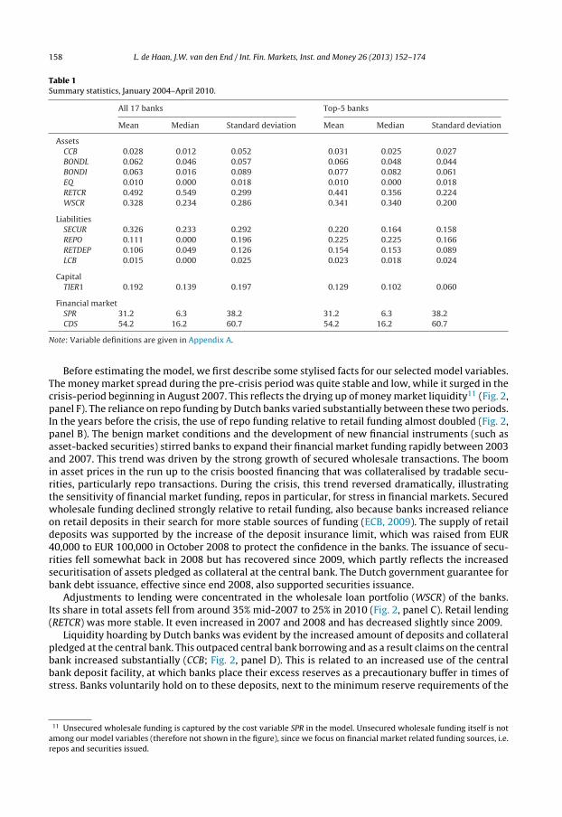
The asset side of the balance sheets is dominated by retail and wholesale loans (Table 1). On theliability side of the balance sheet, retail borrowing accounts for only a small portion (on average10–15%). This is due to the relatively limited retail savings market in the Netherlands, where bankshave to compete with pension funds and insurers (DNB, 2010). Our two samples mostly differ withregard to their reliance on asset market related wholesale funding. The largest 5 banks are moredependent on the repo market, with a share of secured wholesale borrowing (REPO) in total fundingtwice as high compared to the average of 17 banks. The smaller banks are relatively more dependenton the issuance of securities (bonds, commercial paper, certificates of deposits, including asset-backedsecurities), as reflected in the average share of SECUR of 32.6% for the whole sample of 17 banks versus22.0% for the top-5 banks.

8 Levin et al. (2002) t-tests are reported in Appendix B.1. Excluding panel means and time trends, unit roots for all series canbe rejected.

9 The bond index changed around 5% in the sample period while the equity index declined 40–50%, so de facto only theadjustment for EQ has a material impact.

10 The total number of banks under supervision at the end of March 2010 was 81.


Table 1Summary statistics, January 2004–April 2010.

All 17 banks Top-5 banks

Mean Median Standard deviation Mean Median Standard deviation

AssetsCCB 0.028 0.012 0.052 0.031 0.025 0.027BONDL 0.062 0.046 0.057 0.066 0.048 0.044BONDI 0.063 0.016 0.089 0.077 0.082 0.061EQ 0.010 0.000 0.018 0.010 0.000 0.018RETCR 0.492 0.549 0.299 0.441 0.356 0.224WSCR 0.328 0.234 0.286 0.341 0.340 0.200

LiabilitiesSECUR 0.326 0.233 0.292 0.220 0.164 0.158REPO 0.111 0.000 0.196 0.225 0.225 0.166RETDEP 0.106 0.049 0.126 0.154 0.153 0.089LCB 0.015 0.000 0.025 0.023 0.018 0.024

CapitalTIER1 0.192 0.139 0.197 0.129 0.102 0.060

Financial marketSPR 31.2 6.3 38.2 31.2 6.3 38.2CDS 54.2 16.2 60.7 54.2 16.2 60.7

Note: Variable definitions are given in Appendix A.

Before estimating the model, we first describe some stylised facts for our selected model variables.The money market spread during the pre-crisis period was quite stable and low, while it surged in thecrisis-period beginning in August 2007. This reflects the drying up of money market liquidity11 (Fig. 2,panel F). The reliance on repo funding by Dutch banks varied substantially between these two periods.In the years before the crisis, the use of repo funding relative to retail funding almost doubled (Fig. 2,panel B). The benign market conditions and the development of new financial instruments (such asasset-backed securities) stirred banks to expand their financial market funding rapidly between 2003and 2007. This trend was driven by the strong growth of secured wholesale transactions. The boomin asset prices in the run up to the crisis boosted financing that was collateralised by tradable secu-rities, particularly repo transactions. During the crisis, this trend reversed dramatically, illustratingthe sensitivity of financial market funding, repos in particular, for stress in financial markets. Securedwholesale funding declined strongly relative to retail funding, also because banks increased relianceon retail deposits in their search for more stable sources of funding (ECB, 2009). The supply of retaildeposits was supported by the increase of the deposit insurance limit, which was raised from EUR40,000 to EUR 100,000 in October 2008 to protect the confidence in the banks. The issuance of secu-rities fell somewhat back in 2008 but has recovered since 2009, which partly reflects the increasedsecuritisation of assets pledged as collateral at the central bank. The Dutch government guarantee forbank debt issuance, effective since end 2008, also supported securities issuance.

Adjustments to lending were concentrated in the wholesale loan portfolio (WSCR) of the banks.Its share in total assets fell from around 35% mid-2007 to 25% in 2010 (Fig. 2, panel C). Retail lending(RETCR) was more stable. It even increased in 2007 and 2008 and has decreased slightly since 2009.

Liquidity hoarding by Dutch banks was evident by the increased amount of deposits and collateralpledged at the central bank. This outpaced central bank borrowing and as a result claims on the centralbank increased substantially (CCB; Fig. 2, panel D). This is related to an increased use of the centralbank deposit facility, at which banks place their excess reserves as a precautionary buffer in times ofstress. Banks voluntarily hold on to these deposits, next to the minimum reserve requirements of the

11 Unsecured wholesale funding is captured by the cost variable SPR in the model. Unsecured wholesale funding itself is notamong our model variables (therefore not shown in the figure), since we focus on financial market related funding sources, i.e.repos and securities issued.


Fig. 2. Development of model variables.

Eurosystem, which are quite stable at 2% of short-term bank liabilities. The rising share of highly liquidbonds in the total bond portfolio also indicates that Dutch banks hoarded liquidity in the crisis. Theshare of liquid bonds doubled between 2007 and 2010 to nearly 10%. Holdings of less liquid bonds alsoincreased between end-2008 and the beginning of 2010 (BONDI in panel E). This development partlyrelates to securitisation of loans. Since banks were no longer able to place securitised assets in themarket during the crisis, they retained these (asset-backed) securities on their balance sheets for lateruse as collateral when borrowing from the central bank. The Eurosystem made it easier to borrow by


providing unlimited liquidity through fixed rate full allotment from October 2008, extending the listof eligible collateral and lengthening the maturities of LTROs to six and twelve months (ECB, 2010b).

Fig. 2, panel E, shows the development of bond and equity portfolios, adjusted for revaluations.The decline of equity and bond portfolios between mid-2007 and mid-2008 reflects an active scalingdown of these exposures, possibly reflecting fire sales.

5. Results

In this section four p-VAR models are estimated. The first three are designed to capture three typesof bank asset reallocation after a shock in funding liquidity, i.e. (1) a cut in lending, (2) liquidity hoard-ing, and (3) fire-sales. As an encore, a fourth model is estimated designed to test a fourth hypothesis,i.e. whether fire sales are triggered by solvency constraints. As is usual in VAR-studies, results arepresented in the form of impulse responses, including confidence bands. The estimated coefficientsare given in Appendixes.

Results are discussed for the sample of 17 banks and for the sub-sample of the 5 largest banks.However, we only display the results for the sub-sample of 5 banks if they are materially differentfrom those of the full sample of 17 banks.

5.1. Response of lending

In the bank lending model, the variables in vectors X and Y of model (1) are:

[SPR REPO RETDEP WSCR RETCR]′

For bank lending we consider two main categories, wholesale lending (WSCR) and retail lending(RETCR). By also taking two main funding sources into account, i.e. secured wholesale borrowing (REPO)and retail deposits (RETDEP), we model credit management in relation to funding liquidity. With theinclusion of the money market spread (SPR), the model incorporates the price of bank funding, whichalso determines bank lending rates. Hence, the model captures both credit demand and credit supplyeffects. The price of funding is assumed to affect credit demand. When the interbank spread (SPR)rises, banks pass the increased funding costs on to their customers by raising lending rates. As aconsequence, the demand for credit may fall according to the traditional interest rate channel ofmonetary transmission.12 Credit supply effects are assumed to originate from changes in the availablevolume of financial market related wholesale funding, i.e. repo and securities funding. When banksare rationed on the funding market, they have less means to support their asset side activities. As aconsequence, they may curtail lending according to the liquidity channel of financial transmission.

We allow retail deposits to be immediately affected by the stress in the wholesale funding market,while any feedback effect is assumed to occur only with a lag. The response variable of interest is banklending, which is split into wholesale lending and retail lending, of which wholesale lending comesfirst. Robustness checks indicate that changes in the ordering of the variables have no substantial effecton the results.

From the impulse responses (Fig. 3) it appears that wholesale lending (WSCR) reacts significantlyand positively to a shock in secured wholesale funding (REPO) and significantly and negatively to ashock in the money market spread (SPR).13 This applies both to the sample of 17 banks and the sub-sample of the 5 largest banks, and is in line with the experience in the 2007–2009 financial crisis thatwholesale loans were most vulnerable to funding liquidity risk (ECB, 2010a). A sudden rise of interbankspreads and/or constraints in repo funding urge banks to adjust their asset side quickly, both in termsof size and in terms of risk. It is plausible, and evident from the data (Fig. 2, panel B), that banks realisethis adjustment by changing their wholesale lending rather than their retail lending, since in general

12 As a robustness check, we also try an alternative control variable for credit demand effects, i.e. real GDP growth (see Section7).

13 The estimated coefficients are reported in Appendix B.2. The impulse response is also economically substantial: a 1% pointdecrease in REPO can be calculated to lead to a 0.8 percentage point decrease in WSCR.


Fig. 3. Adjustment of lending, sample of 17 banks.


the former has a shorter maturity and a higher risk profile than the latter. This outcome is consistentwith the theoretical framework of Huang and Ratnovski (2011), who show that negative market signalsare an incentive for wholesale financiers to withdraw from lending, especially short-term interbanklending. Liedorp et al. (2010) establish the channel of contagion running from wholesale funding tointerbank lending empirically.

As shown in panel E of Fig. 3, the impulse responses show a significantly negative response of retaillending (RETCR) to a shock in wholesale lending (WSCR). This suggests that, after a shock in the repomarket, banks reduce the share of wholesale loans in their loan book in favour of (lower risk) retailloans. This substitution effect is weaker for the top-5 banks, possibly because the largest banks havea more diversified asset side and therefore more flexibility to adjust their balance sheets. For bothgroups of banks, retail lending (RETCR) shows a brief but significantly positive response to a shockin retail deposits (RETDEP; Fig. 3, panel D). This reflects the linkage between both retail items in theasset and liability management of banks. By matching retail lending with retail deposits, banks limitthe retail funding gap and thereby their dependence on volatile wholesale markets for funding. Undervolatile market conditions, banks shift their funding to more stable retail deposits, as is shown by thesignificant positive response of RETDEP to a shock in SPR (Fig. 3, panel H). Such behaviour of banks wasevident in the crisis, when several Dutch banks attracted more retail deposits by offering relatively highdeposit rates.14. This supply effect was reinforced by customers’ preferences for safe bank deposits.The response of RETDEP is only marginally significant for the top-5 banks, which again underlines thatthese banks have access to a wider range of non-retail funding possibilities than smaller banks.

5.2. Liquidity hoarding

The variables in the model for liquidity hoarding are:

[SPR REPO LCB BONDL CCB]

Liquidity hoarding is captured by highly liquid bonds (BONDL) and claims on the central bank (CCB).Both can act as liquidity buffer in times of stress. By relating these two variables to REPO the linkbetween liquidity hoarding and market dependent funding sources can be investigated. The variableSPR takes into account the influence of funding costs on the unsecured interbank market. Liabilitiesto the central bank (LCB) are included, being the counterpart of claims to the central bank (CCB). Thisallows us to distinguish between borrowing from the central bank (LCB) and liquidity hoarding at thecentral bank (CCB). The funding variables come first in the ordering of the p-VAR. By implication ofthe ordering, the money market spread has an immediate effect on repo borrowing and central bankborrowing, while any feedback effects are assumed to occur only with a lag. The response variable ofinterest is liquidity holdings, which is split into highly liquid bonds and claims on the central bank.

The impulse responses (Fig. 4) indicate that liquidity hoarding is evident in response to a shock inrepo funding.15 For both samples of banks BONDL shows a (short) significant and negative reactionto a shock in secured borrowing (REPO; see Fig. 4, panels B and H), indicating that a disruption in thesecured funding market is followed by an accumulation of highly liquid assets.16 This is in accordancewith the experience during the crisis, when at some point only high-quality collateral was acceptedfor repo transactions, which stimulated the hoarding of such assets. There is also significant evidenceof liquid bond hoarding in response to an upward shock in the money market spread (SPR) by the top-5 banks (Fig. 4, panel G). We find no empirical evidence for feedback effects running from liquidityhoarding to the money market spread; the response of SPR to a shock in BONDL is not significant (resultnot shown in the figure).

The accumulation of central bank reserves (CCB) shows a brief positive response to a shock in themoney market spread (SPR) for both samples (see Fig. 4, panels C and I). Hence, the price of funding

14 The margin between household saving rates and 3 month Euribor increased from −30 basis points in early 2008 to around+200 basis points in early 2010.

15 The estimated coefficients are reported in Appendix B.3.16 The impulse response is economically not very substantial: a 1% point decrease in REPO can be calculated to lead to a 0.1%

point increase in BONDL.


Fig. 4. Liquidity hoarding.

liquidity appears to be an incentive for precautionary savings at the central bank. This is in line withthe theoretical model of Gale and Yorulmazer (2011), according to which the price of liquidity is anincentive to hoard liquidity. Borrowing from the central bank (LCB) shows a similar positive responseto a shock in the money market spread (Fig. 4, panels E and K). This indicates precautionary borrowingby banks in times of stress. Apparently, the funds that were borrowed from the central bank were(partly) stored as deposits at the central bank as the safest storage of liquid assets. The largest banksborrowed and deposited relatively more at the central bank than the other banks in the sample (seeTable 1).

Banks also hoard central bank deposits in response to a shock in repo funding; the impulse responsein panel D of Fig. 4 is significantly negative. This is in accordance with the liquidity hoarding hypothesis,which assumes a negative response of CCB to a shock in REPO (e.g. decline in repo funding stimulatesbanks to hoard central bank reserves). However, the central bank deposits (CCB) of the 5 largest banksdo not show a significant response to a shock in REPO. The big banks might feel less need to hoard


central bank liquidity when repo funding dries up, being less worried to loose market access becauseof their diversified funding base.

5.3. Fire sales

The variables in the model for fire sales are:

[SPR REPO SECUR BONDI EQ ]′

The first three variables are identical to the ones in the liquidity hoarding specification. The responsevariable of interest is securities holdings, which is split into less liquid bonds (BONDI) and equityinvestments (EQ). We include BONDI instead of BONDL (which we used in the liquidity hoarding model),assuming that under stressful market conditions banks prefer to sell their least liquid bonds (BONDI)first, while holding on to their highly liquid bonds (BONDL) for precautionary reasons.

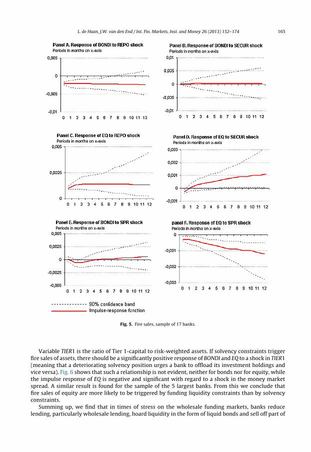
The impulse responses in Fig. 5 do not show a significant response of investment portfolios toshocks in securities issued (SECUR; Fig. 5, panels B and D), but the significant positive response of equityholdings to a shock in secured wholesale funding (REPO; panel C) is consistent with the occurrence offire sales (this result is robust to changing the ordering of the variables in the VAR, while the sampleof the 5 largest banks shows a similar impulse response).17 The positive relation between equityholdings and secured funding may also reflect the use of equities in private repos and securities lendingtransactions. When these activities are buoyant, banks equity holdings are useful as collateral, whilesuch holdings become less useful when the secured funding market collapses and only high-qualitybonds are accepted as collateral. In transactions with the central bank (ECB) equities are not eligible forrefinancing operations. Fixed income assets (like bonds) are eligible collateral if they fulfil particularcriteria (ECB, 2011). The significant negative response of EQ to an upward shock in the money marketspread (SPR) confirms the risk of fire sales after a shock in wholesale funding (panel F). This findingis in line with the results of Nyborg and Östberg (2010), that tightness in the interbank market forliquidity leads banks to pull-back liquidity, i.e. recovering the liquidity granted to a counterparty byselling equity portfolios, among other things. They conclude that this could be either due to directsales of equity holdings by banks or to sales by other stock market investors that are confronted by areduced liquidity supply of banks.

Surprisingly, there is a negative response of less liquid bond holdings (BONDI) to a shock in securedwholesale funding (Fig. 5, panel A), while there is no significant ‘fire sales effect’ for bonds in responseto a shock in the funding spread (panel E). The same result – not shown in the figure – is found whenless liquid bonds (BONDI) are replaced by highly liquid bonds (BONDL), suggesting that banks do notdistinguish between liquid and illiquid bonds when they adjust their bond portfolio in response to afunding shock. Apparently, the liquidity hoarding motive (i.e. an increase of liquid bond holdings aftera negative funding shock, cf. Section 5.2) dominates the fire sale motive with regard to bond portfolios.A reason for this dominance could be the additional liquidity supplied by the central bank during thecrisis, which enabled banks to obtain funding against liquid and less liquid bonds as collateral.18 Bythese liquidity operations, central banks mitigated the adverse consequences of fire sales of assets infinancial markets by banks (ECB, 2010a). By this, central banks complemented the market when itfailed to function.

As pointed out in Section 2, theoretical models (e.g. Cifuentes et al., 2005) and simulation models(e.g. Aikman et al., 2009) are not clear about the issue whether liquidity or capital constraints are themain trigger for fire sales. Therefore, we also estimate a fourth model that relates securities holdingsto both bank capital and the money market spread:

[SPR TIER1 BONDI EQ ] ′

17 The estimation results are reported in Appendix B.4. The impulse response of EQ to REPO is economically not very substantial:a 1% point decrease in REPO can be calculated to lead to a 0.1% point decrease in EQ.

18 The Eurosystem provided unlimited liquidity through fixed rate full allotment from October 2008 and extended the listof eligible collateral, by including lower rated assets, debt instruments denominated in other currencies than euro and debtinstruments issued by credit institutions, such as CDs.


Fig. 5. Fire sales, sample of 17 banks.

Variable TIER1 is the ratio of Tier 1-capital to risk-weighted assets. If solvency constraints triggerfire sales of assets, there should be a significantly positive response of BONDI and EQ to a shock in TIER1(meaning that a deteriorating solvency position urges a bank to offload its investment holdings andvice versa). Fig. 6 shows that such a relationship is not evident, neither for bonds nor for equity, whilethe impulse response of EQ is negative and significant with regard to a shock in the money marketspread. A similar result is found for the sample of the 5 largest banks. From this we conclude thatfire sales of equity are more likely to be triggered by funding liquidity constraints than by solvencyconstraints.

Summing up, we find that in times of stress on the wholesale funding markets, banks reducelending, particularly wholesale lending, hoard liquidity in the form of liquid bonds and sell off part of


Fig. 6. Fire sales and solvency, sample of 17 banks.

their investment portfolio, especially equity. We also find that fire sales are more likely to be triggeredby funding liquidity constraints than by solvency constraints.

6. Is there causality between the behavioural responses?

It is conceivable that a reaction of banks in one market segment may cause adjustments in othermarkets. For example, fire sales may depress bank assets’ market values, which may reduce theircapacity and/or willingness to lend. Liquidity hoarding may lead to cuts in credit lines. Conversely, areduction in wholesale lending may be an incentive for liquidity hoarding or fire sales by banks thatare in need of liquidity but that are not able to borrow from other banks.

In this section, we test for causalities between lending, liquidity hoarding, and fire sales. Specif-ically, for each individual bank, we conduct two-way Granger causality tests between pairs of thevariables that show a significant and/or expected impulse response in the previous section. We reportresults for lags of 3 and 6 months, respectively. The results for 3 and 6 lags (Table 2) indicate thatfor 8 and 6 banks, respectively, there is a significant causality running from fire sales to wholesalelending (from EQ to WSCR). This suggests that fire sales for these banks exert a negative impact onbalance sheets, reducing their capacity and/or willingness to lend, in particular to higher risk (whole-sale) customers. For 6 lags, there is also a causality for 6 banks running from fire sales to liquidityhoarding (from EQ to BONDL), suggesting that banks in need of liquidity sell equity and use theproceeds to purchase liquid bonds. We note, however, that the numbers of banks for which thesesignificant causalities are found, are relatively small compared to the total number of banks in thesample.

Summing up, we find some weak evidence that causality in bank behaviour runs from fire sales ofequity to wholesale lending and liquidity hoarding.


Table 2Granger causality tests.

Lag(3) Lag(6)

Causalitya Sampleb Causalitya Sampleb

WSCR ⇒ BONDL 1 14 0 14BONDL ⇒ WSCR 4 14 2 14WSCR ⇒ EQ 3 13 2 13EQ ⇒ WSCR 8 17 6 17BONDL ⇒ EQ 2 13 2 13EQ ⇒ BONDL 4 14 6 14

a Number of banks for which the H0 of no causality could be rejected at a significance level of 5%.b Number of banks for which the test could be performed.

7. Robustness

In this section we present some robustness tests.19 First, we re-estimate the models for the 12smaller banks in our sample of 17 banks. Concerning the lending model the only notable differenceis that retail credit does not significantly respond to shocks in SPR and REPO, which suggests thatcredit supply by the smaller banks is less sensitive to developments in wholesale funding markets.The impulse responses for the liquidity hoarding model are in line with the findings for the wholesample. The response of central bank reserves (CCB) to repo funding (REPO) and funding cost (SPR)shocks is even stronger for the 12 banks than for the whole sample, suggesting that the smaller banksare more dependent on the central bank for liquidity. With regard to the fire sales model, the responseof equity holdings (EQ) to a shock in the money market spread (SPR) and secured wholesale funding(REPO) is not found to be significant for the smaller banks (compared to the significant response forthe whole sample of banks). One possible explanation for this difference is that the smaller banks inthe Netherlands hold less equity in their trading books and more equity in the form of participationsthat can be sold less easily. A shock to the capital ratio has no significant effect on equity or bondholdings, similar to the result for the whole sample of banks.

Second, we re-estimate the models for a sub-period representing the financial crisis (June 2007to the last month in the dataset, April 2010).20 The impulse responses for the lending model showsome notable differences. The response of wholesale lending (WSCR) to a shock in secured wholesalefunding (REPO) is stronger for the crisis period. This can be explained by the strong adverse shocks tothe wholesale funding market during the crisis. At the peak of the crisis in September/October 2008,repo funding of Dutch banks dropped by almost 1 standard deviation on average for two monthsin a row. For comparison: all impulse response functions show a 1 standard deviation shock duringone single month. The results of the liquidity hoarding and fire sales models for the crisis period arecomparable to the results presented in Sections 5.2 and 5.3 for the whole sample.

Third, we test the robustness of the results for bank lending for the choice of the control variable forcredit demand. Specifically, we replace the interest rate spread (SPR) by real GDP growth (quarter-on-quarter change). Economic growth can be considered to be another driver of credit demand, alternativeto the interest rate spread (SPR).21 The impulse responses indicate that a shock in GDP growth has nosignificant effects on either retail or wholesale lending, in contrast to the significant effects of a shockin SPR to lending (see Section 5.1). However, controlling for credit demand by GDP growth insteadof SPR does not materially change the impulse responses of retail and wholesale lending to a shockin repo funding or retail deposits (which we interpreted as credit supply effects in Section 3). Thissuggests that the credit supply effects are robust to different variables that control for credit demand.

19 For reasons of space, the results of the robustness tests, with the exception of the second robustness test, are not presentedin figures or tables, but they are available on request.

20 The coefficient estimates are presented in Appendix B.5.21 The use of real GDP growth as a control variable for loan demand is common in e.g. the extensive empirical literature on

the credit channel (e.g. Kashyap and Stein, 2000; De Haan, 2003), where bank loan supply effects are examined. A tight relationbetween wholesale lending and GDP growth is also confirmed in studies such as Sørensen et al. (2009).


Fourth, we introduce a variable to the VAR specifications to test for the influence of the defaultrisk of the banks. This risk is reflected in the credit default swap spread (CDS, see Fig. 2, panel F)22

which replaces the money market spread variable (SPR) in the model specifications. In all models, CDSis included as the first variable, assuming that market prices are more exogenous to banks than theirown balance sheets. In general, the results are similar to those of the original model specificationsincluding SPR. A notable difference in the model for bank lending is that the response of wholesalecredit to a shock in CDS is not significant for the whole sample of banks, while it is significantly negativeif SPR is included instead of CDS (see Section 5.1). This suggests that wholesale lending is to a largerextent driven by funding liquidity risk than by banks’ default risk. A similar conclusion can be drawnwith regard to the response of equity holdings in the fire sales model, which is significant for a shockin SPR (see Section 5.3), but not significant for a shock in CDS (this difference is specifically due tothe largest 5 banks). This is in line with the result found in Section 5.3, i.e. that liquidity constraintsrather than solvency constraints seem to trigger sales of equity holdings. A difference in the liquidityhoarding model is that the response of central bank reserves (CCB) to a shock in secured wholesaleborrowing (REPO) is no longer significant. There is a significantly positive response of CCB to CDS,though, suggesting that stress in financial markets (reflected in a higher CDS) goes in tandem withincreased demand for central bank reserves (reflected in an increase of CCB).

8. Conclusion

This paper provides empirical evidence on banks’ responses to funding liquidity shocks, using dataof seventeen of the largest Dutch banks over the period January 2004 to April 2010. The dynamicinterrelations among instruments of bank liquidity management are modelled in a panel VectorAutoregressive (p-VAR) framework. Orthogonalized impulse responses reveal that banks respond to anegative funding liquidity shock in a number of ways. First, banks reduce lending, especially wholesalelending. Wholesale loans are most vulnerable to funding liquidity risk and banks adjust their whole-sale lending rather than their retail lending that generally has longer maturity. Second, banks hoardliquidity, in the form of liquid bonds and central bank reserves. A disruption of the secured fund-ing market is followed by an accumulation of highly liquid assets and the price of funding liquidityappears to be an incentive for precautionary savings at the central bank. Third, banks conduct fire salesof securities, especially equity. With regard to bond holdings, the liquidity hoarding motive seems todominate the fire sale motive when the central bank supplies additional liquidity during the crisis,enabling banks to obtain funding against bonds as collateral. We also find that fire sales are triggeredby liquidity constraints rather than by solvency constraints.

These results have two important policy implications. First, the results confirm that extendedliquidity operations by the central bank can effectively complement the market when it fails to func-tion in a crisis. Central bank deposits provide banks with a precautionary liquidity buffer, while theadditional liquidity supply of the central bank enable banks to obtain funding against collateral (of lessliquid bonds such as asset-backed securities) that is otherwise not eligible for private repo transac-tions. By doing this, the central bank can prevent costly fire sales by banks with too much reliance onwholesale funding. This underlines that a flexible collateral framework of central banks, which can bebroadened in times of stress, is an important safeguard against banks’ responses that destabilise finan-cial markets. Second, the results support the proposal by the Basel Committee to enhance the quantityand quality of liquidity buffers of banks and to reduce their maturity mismatches (BCBS, 2010). Ourresults show that shocks to wholesale funding can induce major adjustments of banks’ balance sheetsthat can be costly for the economy and destabilise financial markets. It may be assumed that banks withmore and higher-quality liquid buffers respond less strongly to shocks in financial markets. Our resultsparticularly support the requirement of the Basel Committee to increase liquidity buffers mostly forbanks with a strong reliance on wholesale funding.

22 For the 12 smaller banks CDS spreads are not available. Therefore, for those banks we use the average CDS spreads of thefive largest banks.


Appendix A. Variable names and definitions

Name Definition

Assetsa

CCB Claims on central bank (deposits at the Eurosystem)BONDL Liquid bond holdings (debt instruments consisting of marketable debt instruments which fulfil

uniform euro area-wide eligibility criteria). Bonds are reported at current market values. In thepaper we deflated the value by the FTSE EURO index of corporate bonds

BONDI Less liquid bond holdings (debt instruments consisting of marketable and nonmarketable assetswhich are of particular importance for national financial markets and banking systems. Theeligibility criteria for these assets are established by the national central banks, subject to theminimum eligibility criteria established by the ECB). Bonds are reported at current market values.In the paper we deflated the value by the FTSE EURO index of corporate bonds

EQ Equity portfolio (quoted and non-quoted equities). Stocks are reported at current market values.In the paper we deflated the value by the MSCI worldwide stock index

RETCR Retail credit (credit claims outstanding to households and companies)WSCR Wholesale credit (secured and unsecured credit claims outstanding to professional counterparties)

Liabilitiesa

SECUR Securities issued (consisting of debt instruments, such as bonds, CPs, CDs and subordinatedliabilities)

REPO Secured wholesale borrowing (amounts related to repo, reverse repo and securities borrowingtransactions other than with central banks, secured by debt instruments or equity)

RETDEP Retail deposits (fixed-term and demand deposits of households and smaller companies)LCB Liabilities to central bank (borrowing from the Eurosystem through main refinancing operations

and long-term refinancing operations)

CapitalTIER1 Ratio of Tier 1 capital to risk-weighted assets

Financial marketsSPR Money market spread (spread between 3-month Euro Interbank Offer Rate (Euribor) and

overnight Euro Interbank Offer Rates (Eonia) swap index), in basis pointsCDS Credit default swap spread, in basis points (average 5-year CDS spreads of five largest financial

institutions in the Netherlands)a Ratios to total assets.

Appendix B.

B.1. Levin et al. (2002) unit-root tests

Ho: Panels contain unit rootsHa: Panels are stationary

Panel means: Included Included Not includedTime trend: Not included Included Not included

Variable Adjusted t p-Value Adjusted t p-Value Adjusted t p-Value

SPR −4.54 0.00 −5.80 0.00 −8.63 0.00REPO −0.81 0.21 −0.30 0.38 −4.28 0.00RETDEP −2.22 0.01 −0.08 0.47 −4.25 0.00WSCR −2.65 0.00 −2.03 0.02 −5.39 0.00RETCR −2.94 0.00 −4.34 0.00 −5.56 0.00SECUR −0.02 0.49 −0.61 0.27 −4.04 0.00LCB 0.22 0.56 −0.92 0.82 −5.25 0.00BONDL −2.66 0.00 −2.69 0.01 −5.55 0.00CCB −3.71 0.00 −4.65 0.00 −5.73 0.00BONDI −1.64 0.05 −2.41 0.01 −4.94 0.00EQ −0.71 0.24 −0.53 0.30 −4.60 0.00TIER1 −3.58 0.00 −5.69 0.00 −5.69 0.00

ADF regressions: 1 lag; AR parameter: Common.LR variance: Bartlett kernel, 13.00 lags average (chosen by LLC).


B.2. Estimation results for lending, period January 2004–April 2010

Explanatory variables Dependent variables

SPR REPO RETDEP WSCR RETCR

Panel A: sample of 17 banksSPR (t-1) 1.26*** (36.72) −0.00 (−1.12) 0.00*** (3.18) −0.00*** (−2.68) 0.00** (2.45)SPR (t-2) −0.58*** (−13.39) 0.00 (−0.32) −0.00 (−1.47) 0.00 (1.13) 0.00* (−1.72)SPR (t-3) 0.27*** (13.56) 0.00 (0.72) 0.00 (1.12) 0.00 (0.00) 0.00 (0.84)REPO (t-1) −38.04 (−0.92) 1.03*** (10.45) 0.00 (0.02) 0.21*** (2.64) −0.09* (−1.73)REPO (t-2) 37.48 (0.77) 0.01 (0.11) 0.01 (0.27) 0.05 (0.44) −0.02 (−0.32)REPO (t-3) 8.67 (0.34) −0.05 (−0.71) −0.01 (−0.69) −0.24*** (−3.34) 0.90** (2.23)RETDEP (t-1) 51.41 (0.68) −0.05 (−0.63) 0.91*** (10.2) −0.03 (−0.22) −0.12 (−0.85)RETDEP (t-2) 75.78 (1.00) 0.14 (1.55) 0.12 (1.57) 0.09 (0.70) 0.04 (0.37)RETDEP (t-3) −95.41 (−1.24) −0.08 (−1.28) −0.03 (−0.75) −0.048 (−0.45) 0.08 (0.94)WSCR (t-1) 29.24 (1.26) −0.03 (−1.46) 0.03 (1.33) 0.64*** (6.72) 0.44 (0.02)WSCR (t-2) −5.09 (−0.30) 0.09 (0.52) −0.01 (−0.71) 0.01 (0.10) 0.03 (0.09)WSCR (t-3) −26.00 (−1.63) 0.01 (0.70) −0.01 (−1.31) 0.34*** (3.32) −0.03 (−1.28)RETCR (t-1) 48.09 (−1.15) −0.01 (−0.41) 0.00 (0.17) −0.03 (−0.31) 0.81*** (8.88)RETCR (t-2) −14.13 (−0.54) 0.00 (−0.14) 0.00 (0.09) −0.10 (−1.10) 0.09** (2.12)RETCR (t-3) −15.68 (−0.78) 0.00 (−0.15) 0.00 (0.01) 0.09 (1.26) 0.09*** (2.66)

Number of observations 1199

Panel B: sample of top-5 banksSPR (t-1) 1.25*** (23.34) −0.00 (−0.73) 0.00** (2.21) −0.00* (−1.67) 0.00** (2.39)SPR (t-2) −0.55*** (−8.07) 0.00 (0.07) −0.00 (−0.19) −0.00 (−0.17) −0.00 (−0.95)SPR (t-3) 0.25*** (6.81) −0.00 (−0.35) −0.00 (−0.11) 0.00 (0.84) −0.00 (−0.11)REPO (t-1) −11.86 (−0.12) 0.93*** (7.31) −0.00 (−0.06) 0.11 (0.78) −0.14 (−1.60)REPO (t-2) 38.51 (0.63) 0.09 (0.77) 0.01 (0.14) 0.15 (1.34) −0.09 (−0.91)REPO (t-3) 114.48 (1.37) −0.11 (−0.82) 0.00 (0.03) −0.22* (−1.73) 0.29** (2.53)RETDEP (t-1) 151.13 (1.04) 0.01 (−0.63) 0.91*** (12.71) 0.09 (0.44) −0.34* (−1.72)RETDEP (t-2) 278.80 (0.95) 0.22 (1.16) 0.12 (1.35) 0.01 (0.05) 0.15 (0.63)RETDEP (t-3) −387.36 (−1.15) −0.13 (−1.14) −0.06 (−0.74) −0.09 (−0.43) 0.18 (0.89)WSCR (t-1) 57.85 (0.59) 0.04 (0.28) 0.03 (0.66) 0.66*** (5.02) 0.18* (1.66)WSCR (t-2) −36.99 (−0.38) 0.00 (0.02) −0.03 (−0.78) 0.14 (1.14) −0.08 (−0.72)WSCR (t-3) −138.27** (−2.02) 0.04 (0.32) −0.01 (−0.21) 0.14 (1.34) −0.15* (−1.71)RETCR (t-1) 45.58 (0.73) 0.05 (0.53) −0.02 (−0.55) 0.03 (0.29) 0.91*** (10.36)RETCR (t-2) −44.82 (−0.55) 0.66 (−0.55) 0.02 (0.82) 0.05 (0.43) −0.09 (−0.84)RETCR (t-3) 48.86 (0.86) 0.02 (0.19) −0.01 (−0.20) −0.11 (−1.06) 0.18 (2.11)


Panel VAR model estimation by GMM, with fixed effects removed prior to estimation (see Section 3 for details).Heteroskedasticity adjusted t-statistics within parentheses.

* Significance at 10% level.** Significance at 5% level.

*** Significance at 1% level.

B.3. Estimation results for liquidity hoarding, period January 2004–April 2010


SPR REPO LCB BONDL CCB

Panel A: sample of 17 banksSPR (t-1) 1.24*** (18.80) −0.00 (−0.89) −0.00 (−0.27) 0.00 (0.13) 0.00 (0.14)SPR (t-2) −0.57*** (−14.02) −0.00 (−0.21) −0.00 (−0.17) 0.00* (1.71) −0.00 (−0.40)SPR (t-3) 0.25*** (9.36) 0.00 (0.26) −0.00 (−0.17) −0.00* (−1.65) −0.00 (−1.03)REPO (t-1) −33.07 (−0.70) 1.00*** (10.81) 0.00 (0.09) −0.00 (−0.05) −0.11 (−1.28)REPO (t-2) 40.18 (0.83) 0.01 (0.07) −0.02 (−1.09) −0.01 (−0.14) −0.02 (−0.23)REPO (t-3) 4.89 (0.22) −0.03 (−0.44) 0.01 (0.75) 0.01 (0.22) 0.09 (1.39)LCB (t-1) 50.82 (1.11) 0.05 (0.96) 0.85*** (11.14) 0.01 (0.21) 0.08 (0.72)LCB (t-2) −0.50 (−0.01) 0.07 (0.82) 0.05 (0.59) −0.11 (−1.29) 0.13 (0.95)LCB (t-3) −43.15 (−0.77) −0.08 (−0.92) 0.04 (0.46) 0.13 (1.50) −0.05 (−0.32)BONDL (t-1) −95.46 (−0.82) 0.01 (0.07) −0.07 (−0.76) 0.91*** (7.64) −0.14 (−0.41)




BONDL (t-2) 36.96 (1.24) −0.01 (−0.31) 0.00 (0.01) 0.04 (0.58) −0.05 (−0.76)BONDL (t-3) −1.02 (−0.04) −0.01 (−0.33) −0.03 (−1.02) 0.07 (1.62) 0.01 (0.15)CCB (t-1) 23.69 (1.14) −0.01 (−0.41) 0.02 (1.24) −0.00 (−0.30) 0.63*** (5.47)CCB (t-2) −13.02 (−0.68) −0.00 (−0.35) 0.00 (0.01) 0.02 (1.37) −0.06 (−0.34)CCB (t-3) 27.12* (1.97) 0.00 (0.10) −0.00 (−0.31) −0.01 (−1.01) 0.40*** (2.75)


Panel B: sample of top-5 banksSPR (t-1) 1.19*** (15.35) −0.00* (−1.63) 0.00* (1.49) −0.00 (−0.07) 0.00 (0.34)SPR (t-2) −0.54*** (−7.94) 0.00 (0.37) −0.00** (−1.89) 0.00** (2.66) −0.00 (−1.19)SPR (t-3) 0.28*** (6.65) −0.00 (−0.76) 0.00 (0.54) −0.00** (−2.29) 0.00 (0.94)REPO (t-1) 8.55 (0.16) 0.96*** (10.21) 0.01 (0.31) −0.01 (−0.22) 0.02 (0.59)REPO (t-2) −17.11 (−0.33) 0.10 (0.91) −0.01 (−0.49) 0.01 (0.40) −0.05 (−1.55)REPO (t-3) 66.18** (1.84) −0.06 (−0.85) 0.00 (0.06) −0.01 (−0.45) 0.01 (0.36)LCB (t-1) 301.58 (1.39) 0.45*** (2.56) 0.76*** (11.58) 0.09 (0.57) −0.04 (0.27)LCB (t-2) 448.26*** (2.62) −0.09 (−0.39) 0.05 (0.59) −0.12 (−0.75) 0.00 (0.22)LCB (t-3) 60.65 (0.55) −0.29 (−1.24) 0.17*** (2.23) 0.08 (0.69) 0.05 (0.36)BONDL (t-1) 48.03 (−0.53) −0.12 (−0.99) 0.01 (0.29) 0.77*** (10.11) 0.10 (1.09)BONDL (t-2) −52.67 (−0.45) 0.17 (1.31) −0.00 (−0.06) 0.18*** (2.05) −0.22* (−1.80)BONDL (t-3) 82.65 (1.04) −0.11 (−0.83) −0.02 (−0.41) 0.04 (0.64) 0.09 (1.08)CCB (t-1) 2.22 (0.15) 0.02 (0.15) −0.01 (−0.25) −0.01 (−0.12) 0.70*** (5.26)CCB (t-2) 99.60 (1.38) −0.05 (−0.43) 0.05 (1.44) 0.03 (0.38) 0.12 (1.56)CCB (t-3) 78.09 (1.12) 0.15 (1.52) −0.03 (−0.66) −0.05 (−0.98) 0.14*** (2.21)


VAR model is estimated by GMM, fixed effects are removed prior to estimation (see Section 3 for details).Heteroskedasticity adjusted t-statistics in parentheses.



B.4. Estimation results for fire sales, period January 2004–April 2010


SPR REPO SECUR BONDI EQ

Panel A: sample of 17 banksSPR (t-1) 1.24*** (35.01) 0.00 (−0.75) 0.00*** (−3.06) −0.00** (−2.21) −0.00 (−0.24)SPR (t-2) −0.57*** (−12.82) 0.00 (−0.24) 0.00** (2.42) 0.00 (1.43) 0.00 (0.22)SPR (t-3) 0.27*** (13.29) 0.00 (0.42) −0.00 (−1.61) −0.00 (−0.39) −0.00 (−1.05)REPO (t-1) −50.56 (−1.18) 1.03*** (10.50) −0.05 (−1.57) −0.03 (−0.70) 0.03** (2.00)REPO (t-2) 50.11 (0.97) 0.01 (0.04) 0.05 (1.29) 0.01 (0.16) −0.02 (−0.73)REPO (t-3) −12.82 (−0.68) −0.03 (−0.51) −0.02 (−0.63) 0.01 (0.39) −0.01 (−0.93)SECUR (t-1) −41.71 (−0.64) 0.05 (1.60) 0.73*** (5.08) 0.00 (0.01) 0.02** (2.22)SECUR (t-2) 41.84** (2.49) −0.01 (−0.52) 0.15 (1.20) 0.01 (0.70) −0.00 (−0.54)SECUR (t-3) 3.90 (0.22) −0.01 (−0.49) 0.01 (0.16) −0.01 (−0.71) −0.00 (−0.64)BONDI (t-1) −65.31 (−1.40) 0.09 (1.50) 0.05 (1.05) 0.88*** (15.86) 0.02* (1.89)BONDI (t-2) 77.28 (1.58) −0.07 (−0.87) −0.02 (−0.49) 0.01 (0.07) −0.02 (−1.12)BONDI (t-3) −38.19 (−1.59) −0.03 (−0.43) −0.04 (−0.98) 0.10 (1.09) −0.00 (−0.08)EQ (t-1) −51.69 (−0.28) 0.25 (1.23) −0.18 (−0.95) 0.09 (0.93) 0.88*** (9.71)EQ (t-2) 39.39 (0.20) −0.13 (−0.47) −0.15 (−1.31) 0.06 (0.84) −0.01 (−0.12)EQ (t-3) 137.73 (0.78) −0.03 (−0.10) 0.02 (0.19) −0.08 (−1.22) 0.12 (1.18)


Panel B: sample of top-5 banksSPR (t-1) 1.24*** (21.67) −0.00 (−0.58) −0.00** (−1.82) −0.00 (−1.17) −0.00 (−0.16)SPR (t-2) −0.58*** (−8.37) −0.00 (−0.14) 0.00 (1.58) −0.00 (−0.34) 0.00 (0.34)




SPR (t-3) 0.29*** (7.44) −0.00 (−0.43) 0.00 (0.38) 0.00 (0.25) −0.00 (−1.62)REPO (t-1) −88.14 (−0.72) 0.85*** (6.96) 0.12 (1.01) −0.07* (−1.79) 0.05 (1.49)REPO (t-2) 46.25 (0.67) 0.06 (0.58) 0.03 (0.55) −0.03 (−0.92) −0.04 (−1.02)REPO (t-3) 7.84 (0.23) −0.08 (−1.10) 0.00 (0.06) 0.05** (2.07) −0.03 (−1.06)SECUR (t-1) −235.12** (−2.41) 0.16 (1.21) 1.04*** (10.09) −0.03 (−0.74) 0.05 (1.21)SECUR (t-2) 253.13*** (2.79) −0.25** (−1.86) −0.06 (−0.68) 0.05 (1.04) −0.07 (−1.37)SECUR (t-3) −39.91 (−0.67) −0.02 (−0.19) 0.12 (1.37) −0.05 (−1.30) −0.00 (−0.13)BONDI (t-1) −40.06 (−0.40) −0.07 (−0.46) 0.03 (0.33) 0.58*** (8.60) 0.07 (1.51)BONDI (t-2) 118.99 (0.99) 0.03 (0.24) 0.04 (0.44) 0.25*** (3.11) −0.05 (−1.13)BONDI (t-3) −115.51** (−1.71) −0.04 (−0.31) 0.02 (0.24) 0.12* (1.74) −0.03 (−0.77)EQ (t-1) −15.69 (−0.07) 0.35 (1.53) −0.05 (−0.32) 0.10 (1.47) 0.78*** (8.62)EQ (t-2) 40.34 (0.19) −0.15 (−0.51) −0.27* (−1.79) 0.11 (1.45) 0.00 (0.01)EQ (t-3) 123.54 (0.58) 0.15 (0.56) 0.01 (0.04) −0.10 (−1.51) 0.15 (1.40)


Panel VAR model estimated by GMM, with fixed effects removed prior to estimation (see Section 3 for details).Heteroskedasticity adjusted t-statistics within parentheses.



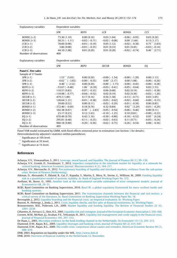
B.5. Estimation results, crisis period June 2007–April 2010


SPR REPO RETDEP WSCR RETCR

Panel A. LendingSample of 17 banks

SPR (t-1) 1.09*** (34.92) 0.00 (0.15) 0.00*** (0.43) −0.00 (−0.30) 0.00** (1.34)SPR (t-2) −0.52*** (−12.40) −0.00 (−0.69) 0.00 (−0.74) 0.00 (0.63) −0.00* (−1.66)SPR (t-3) 0.21*** (9.69) 0.00 (0.70) 0.00 (0.81) 0.00 (0.43) 0.00 (0.88)REPO (t-1) −131.35 (−1.65) 1.08*** (6.00) −0.02 (−0.76) 0.31** (2.13) −0.10 (−1.13)REPO (t-2) 107.57 (1.27) −0.03 (−0.14) 0.01 (0.19) 0.05 (0.29) −0.01 (−0.01)REPO (t-3) −1.19 (−0.03) −0.09 (−1.17) −0.01 (−0.51) −0.30*** (−2.86) 0.07 (1.23)RETDEP (t-1) −240.60 (−0.86) 0.03 (0.19) 0.72*** (3.60) 0.36 (0.84) −0.24 (−0.57)RETDEP (t-2) 105.67 (0.91) 0.28*** (2.68) 0.18** (2.09) 0.17 (0.76) 0.04 (0.27)RETDEP (t-3) −49.82 (−0.28) −0.25** (−2.35) −0.03 (−0.41) −0.24 (−0.97) 0.11 (0.57)WSCR (t-1) 60.08 (1.65) −0.03 (−1.07) 0.01 (0.38) 0.64*** (5.68) 0.03 (0.51)WSCR (t-2) 9.04 (0.33) 0.02 (1.48) −0.02 (−1.15) −0.02 (−0.14) −0.01 (−0.19)WSCR (t-3) −18.52 (−0.77) 0.01 (0.36) 0.00 (0.45) 0.36*** (2.82) 0.00 (−0.14)RETCR (t-1) 86.85 (1.15) 0.01 (0.33) −0.04 (−0.96) 0.10 (0.77) 0.76*** (5.14)RETCR (t-2) −1.38 (−0.03) 0.01 (0.53) −0.03 (−1.35) −0.09 (−0.84) 0.08 (1.45)RETCR (t-3) −5.01 (−0.14) 0.00 (−0.04) 0.00 (0.09) 0.11 (1.14) 0.07 (1.24)




Panel B. Liquidity hoardingSample of 17 banks

SPR (t-1) 1.44*** (7.19) 0.00 (0.71) 0.00 (1.08) −0.00 (−0.42) 0.00 (1.49)SPR (t-2) −0.63*** (−5.91) −0.00 (−0.54) −0.00 (−0.86) 0.00* (1.61) −0.00 (−1.09)SPR (t-3) 0.36*** (3.90) 0.00 (0.40) 0.00 (0.77) −0.00 (−1.30) 0.00 (0.61)REPO (t-1) 8.37 (0.08) 1.05*** (5.90) 0.05 (1.11) −0.01 (−0.24) 0.06 (0.39)REPO (t-2) 136.39 (1.44) −0.03 (−0.15) −0.01 (−0.31) −0.01 (−0.17) −0.01 (−0.06)REPO (t-3) −73.27 (−1.23) −0.07 (−0.84) −0.02 (−0.45) 0.01 (0.27) 0.05 (0.37)LCB (t-1) 57.90 (0.57) 0.00 (0.03) 0.92*** (9.46) 0.02 (0.22) 0.11 (0.55)LCB (t-2) 20.63 (0.17) 0.10 (1.14) −0.05 (−0.47) −0.13 (−1.32) 0.14 (0.70)LCB (t-3) −116.13 (−1.13) −0.08 (−0.82) 0.05 (0.56) 0.15 (1.59) −0.18 (−0.86)BONDL (t-1) 95.99 (0.65) 0.03 (0.33) 0.04 (0.55) 0.90*** (7.64) 0.40 (1.56)



SPR REPO LCB BONDL CCS

BONDL (t-2) 73.36 (1.10) 0.00 (0.16) 0.03 (1.04) −0.06 (−0.95) 0.03 (0.26)BONDL (t-3) 50.31 (−1.11) −0.02 (−0.71) −0.02 (−0.08) 0.09* (1.66) 0.13 (1.17)CCB (t-1) 78.60 (0.98) −0.01 (−0.19) 0.05 (1.12) −0.02 (−0.38) 0.75*** (3.83)CCB (t-2) 3.86 (0.08) −0.01 (−0.35) 0.01 (0.33) 0.01 (0.45) −0.03 (−0.14)CCB (t-3) 44.10 (1.08) 0.01 (0.29) 0.01 (0.28) −0.02 (−0.74) 0.46*** (2.71)




Panel C. Fire salesSample of 17 banks

SPR (t-1) 1.53*** (5.03) 0.00 (0.20) −0.00 (−1.54) −0.00 (−1.20) 0.00 (1.13)SPR (t-2) −0.62*** (−3.82) −0.00 (−0.55) 0.00** (2.17) 0.00 (1.08) −0.00 (−0.26)SPR (t-3) 0.40** (−2.52) 0.00 (0.39) −0.00* (−1.73) −0.00 (−0.45) −0.00 (−0.28)REPO (t-1) −53.67 (−0.48) 1.06*** (6.39) −0.03 (−0.41) −0.05 (−0.64) 0.02 (1.53)REPO (t-2) 110.57 (0.83) −0.07 (−0.33) 0.06 (0.68) 0.02 (0.19) −0.01 (−0.38)REPO (t-3) −110.98 (−0.77) −0.04 (−0.52) 0.02 (0.19) 0.02 (0.30) −0.02 (−1.26)SECUR (t-1) 479.3 (1.00) 0.17 (0.16) 0.56 (1.58) −0.13 (−0.71) 0.03 (1.05)SECUR (t-2) 128.64 (1.31) −0.01 (−0.38) −0.05 (−0.62) −0.02 (−0.60) −0.00 (−0.13)SECUR (t-3) 39.60 (0.52) 0.00 (0.11) −0.02 (−0.29) −0.01 (−0.39) 0.00 (0.85)BONDI (t-1) −372.46 (−0.69) 0.18 (0.76) 0.32 (0.84) 0.92*** (3.29) −0.01 (−0.29)BONDI (t-2) 102.38 (0.67) −0.30*** (−2.83) −0.05 (−0.54) −0.06 (−0.46) 0.00 (0.11)BONDI (t-3) 23.17 (0.23) 0.12 (1.63) −0.10 (−1.25) 0.10 (0.81) −0.00 (−0.23)EQ (t-1) 670.49 (0.70) 0.42 (1.16) −0.50 (−0.80) −0.18 (−0.52) 0.95*** (6.24)EQ (t-2) 295.81 (0.40) −0.11 (−0.25) −0.02 (−0.63) 0.11 (0.71) −0.05 (−0.24)EQ (t-3) 960.18 (0.80) −0.20 (−0.36) −0.62 (−0.75) −0.26 (−0.54) 0.08 (−0.36)


Panel VAR model estimated by GMM, with fixed effects removed prior to estimation (see Section 3 for details).Heteroskedasticity adjusted t-statistics within parentheses.



References

Acharya, V.V., Viswanathan, S., 2011. Leverage, moral hazard, and liquidity. The Journal of Finance 66 (1), 99–138.Acharya, V.V., Gromb, D., Yorulmazer, T., 2012. Imperfect competition in the interbank market for liquidity as a rationale for

central banking. American Economic Journal: Macroeconomics 4 (2), 184–217.Acharya, V.V., Merrouche, O., 2012. Precautionary hoarding of liquidity and interbank markets: evidence from the sub-prime

crisis. Review of Finance (forthcoming).Aikman, D., Alessandri, P., Eklund, B., Gai, P., Kapadia, S., Martin, E., Mora, N., Sterne, G., Willison, M., 2009. Funding liquidity

risk in a quantitative model of systemic stability. In: Bank of England Working Paper No. 372.Arellano, M., Bover, O., 1995. Another look at the instrumental variable estimation of error component models. Journal of

Econometrics 68, 29–51.BCBS, Basel Committee on Banking Supervision, 2010. Basel III: a global regulatory framework for more resilient banks and

banking systems.BCBS, Basel Committee on Banking Supervision, 2011. The transmission channels between the financial and real sectors: a

critical survey of the literature. In: Basel Committee on Banking Supervision Working Paper No. 18.Berrospide, J., 2012. Liquidity hoarding and the financial crisis: an empirical evaluation. In: Working Paper.Boyson, N., Helwege, J., Jinda, J., 2011. Crisis, liquidity shocks, and fire sales at financial institutions. In: Working Paper.Brunnermeier, M.K., Pedersen, L.H., 2009. Market liquidity and funding liquidity. The Review of Financial Studies 22 (6),

2201–2238.Cifuentes, R., Ferrucci, G., Shin, H.S., 2005. Liquidity risk and contagion. Journal of the European Economic Association 3, 556–566.Cornett, M.M., McNutt, J.J., Strahan, P.E., Tehranian, H., 2011. Liquidity risk management and credit supply in the financial crisis.

Journal of Financial Economics 101, 297–312.De Haan, L., 2003. Microdata evidence on the bank lending channel in the Netherlands. De Economist 151 (3), 293–315.Diamond, D.W., Rajan, R.G., 2005. Liquidity shortages and banking crises. Journal of Finance 60 (2), 615–647.Diamond, D.W., Rajan, R.G., 2009. The credit crisis: conjectures about causes and remedies. American Economic Review 99 (2),

606–610.DNB, 2003. Regulation on liquidity under the Wft., http://www.dnb.nlDNB, 2010. Overview of financial stability in the Netherlands 12, November.

http://refhub.elsevier.com/S1042-4431(13)00026-7/sbref0005




















































































































































































































































http://www.dnb.nl/











DNB, 2011. Dutch securitisations back in investors’ favour. DNBulletin.DNB, 2012. Overview of Financial Stability in the Netherlands, March, 15.Doytch, N., Uctum, M., 2011. Does the worldwide shift of FDI from manufacturing to services accelerate economic growth? A

GMM estimation study. Journal of International Money and Finance 30, 410–427.ECB, 2009. EU banks’ funding structures and policies.ECB, 2010a. Report on deleveraging in the EU banking sector.ECB, 2010b. Monthly Bulletin, October.ECB, 2011. General documentation on Eurosystem monetary policy instruments and procedures.French, K.R., et al., 2010. The Squam Lake Report. Princeton University Press, Princeton, NJ.Gale, D., Yorulmazer, T., 2011. Liquidity hoarding. Federal Reserve Bank of New York Staff Report, 488.Heider, F., Hoerova, M., Holthausen, C., 2009. Liquidity hoarding and interbank market spreads: the role of counterparty risk.

In: ECB Working Paper No. 1126.Huang, R., Ratnovski, L., 2011. The dark side of bank wholesale funding. Journal of Financial Intermediation 20 (2), 248–263.IMF, 2010. Systemic liquidity risk: improving the resilience of financial institutions and markets. In: Global Financial Stability

Report, October.Ivashina, V., Scharfstein, D., 2010. Bank lending during the financial crisis of 2008. Journal of Financial Economics 97, 319–338.Kashyap, A., Stein, J., 2000. What do a million observations on banks say about the transmission of monetary policy. American

Economic Review 90, 407–428.Levin, A., Lin, C., Chu, C., 2002. Unit root test in panel data: asymptotic and finite-sample properties. Journal of Econometrics

108, 1–24.Liedorp, F.R., Medema, L., Koetter, M., Koning, R.H., Van Lelyveld, I., 2010. Peer monitoring or contagion? Interbank market

exposure and bank risk. In: DNB Working Paper No. 248.Love, I., Zicchino, L., 2006. Financial development and dynamic investment behaviour: evidence from panel VAR. Quarterly

Review of Economics and Finance 46, 190–210.Nyborg, K.G., Östberg, P., 2010. Money and liquidity in financial markets, Centre for Economic Policy Research. In: Discussion

Paper No. 7905.Shleifer, A., Vishny, R., 2011. Fire sales in finance and macroeconomics. Journal of Economic Perspectives 25 (1), 29–48.Sørensen, C.K., Marques-Ibánez, D., Rossi, C., 2009. Modelling loans to non-financial corporations in the euro area. In: ECB

Working Paper No. 989.Spindt, P.A., Tarfan, V., 1980. Liquidity adjustment behaviour of large money center banks. Journal of Money, Credit and Banking

12 (2), 198–208.Van den End, J.W., Tabbae, M., 2012. When liquidity risk becomes a systemic issue: empirical evidence of bank behaviour.

Journal of Financial Stability 8 (2), 107–120.




























































































































































































































































































































Documents

Banks’ responses to funding liquidity shocks: Lending adjustment, liquidity hoarding and fire sales