Banks as Producers of Financial Services

Wilbur John Coleman II and Christian Lundblad∗

2018-12-30

Abstract

This paper documents that a rise in government debt is associated with a fall

in shadow banking and a rise in traditional banking. This is explained in a model

where banks are valued for the financial services they offer. Government debt does

not compete directly with banks in providing financial services, but the demand for

government debt by banks imparts a liquidity premium to government debt. A rise in

government debt is estimated to disproportionately benefit traditional banks so they

expand at the expense of shadow banks. An optimal debt policy leads both types of

banks to become default free.

∗Duke University (coleman@duke.edu), and The University of North Carolina (Chris-tian Lundblad@kenan-flagler.unc.edu). We wish to thank Ravi Bansal for many helpful comments.

1 Introduction

We begin this paper by documenting that a rise in government debt is associated with

a fall in shadow banking assets and a rise in traditional/commercial banking assets.

The curious positive association between government debt and traditional banking

poses a challenge to a variety of banking models that posit banks’ value stem pri-

marily from their production of safe, liquid assets. If safety per se receives special

value in an economy, and banks are primarily involved in the production of safe as-

sets, then government debt should be a substitute for all types of banking, including

traditional banking. Models of banking that primarily stress the role of banks in pro-

ducing safe, liquid assets include Gorton and Pennacchi (1990), Holmstrom and Tirole

(1998), Krishnamurthy and Vissing-Jorgenson (2012, 2015), Stein (2012), Sunderam

(2014), Greenwood, et. al. (2015), and Diamond (2017) among many others.1 In this

paper we argue that banks’ value stem primarily from their production of a menu of

financial services, albeit services whose expected value depends to a significant extent

on the safety of banks. As it regards government debt, this distinction is important,

as government debt does not per se produce financial services. Focusing on financial

services also provides a natural distinction between traditional and shadow banks in

terms of the menu of financial services each produces. Traditional banks offer a full

menu of check-clearing and electronic transaction services and are meant to accommo-

date high-volume transaction accounts, whereas shadow banks offer more limited free

check-writing features and are meant to satisfy liquidity needs. We show that such a

model is able to explain the different response of traditional and shadow banks to a

change in the supply of government debt. This model is also consistent with a variety

of other features of banking, including how traditional and shadow banks respond in

different ways to a rise in uncertainty. Specifically, with deposit insurance the model

predicts that a rise in uncertainty leads to a shift towards traditional banks and away

from shadow banks, but without deposit insurance the model predicts that a rise in

uncertainty leads to a shift away from both traditional and shadow banks. We validate

this prediction by comparing the behavior of banking during the Great Depression to

the behavior during the 2007/08 Financial Crisis.

In our model, shadow banks emerge in a competitive banking system to compete

with traditional banks to provide financial services. In defining shadow banks, the

model builds on the unique role of banking in offering financial services backed up by

1To be sure, Diamond and Dybvig (1983) stress the safe, liquid aspect of bank deposits, but in theirsetup banks offer risk sharing that differentiates their deposits from government debt from the perspectiveof depositors.

1

holdings of safe assets. Due to their more limited role in providing financial services,

shadow banks find it optimal to hold a somewhat riskier portfolio of assets in com-

parison to traditional banks. Traditional banks, in contrast, offer financial services

such as checkable deposits that depend more on safety and therefore choose to hold

a safer portfolio of assets. In this setup, government debt does not provide financial

services and hence does not compete directly with financial institutions. Rather, fi-

nancial institutions purchase government debt to manage their exposure to risk, which

is especially important for financial institutions as the service they provide depends to

an important degree of the safety of the assets they create. Indeed, if government debt

is in limited supply, the demand for government debt by financial institutions leads to

a liquidity premium in the price of government debt. This liquidity premium is not a

reflection of a financial service offered by government debt or any other riskless asset,

but rather is a reflection of the demand for government debt by financial institutions

that offer financial services that depend to a significant extent on the expectation of

the fulfillment of this service. This distinction is important to understand the value

created by various types of financial institutions and to understand how this value

depends on the supply of government debt.

A rise in the supply of government debt leads to a fall in its liquidity premium that

encourages all financial institutions to hold more of this debt, to become safer, and to

expand. A key insight of this paper is that with a sufficient supply of government debt

to eliminate the liquidity premium on this debt, all financial institutions should become

riskless. Indeed, we show that this is the optimal government debt policy. The relative

size of shadow to traditional banking would then depend entirely on the relative cost

and value of the financial service they offer. Any substitution of traditional banking for

shadow banking as government debt expands from relatively low levels thus depends on

a comparison of how each is able to compete in an environment where they must absorb

risk versus an environment where each becomes riskless. Of course, the situation is

quite different with deposit insurance for traditional banks. With deposit insurance

traditional banks continue to benefit from an expansion of government debt, as the

liquidity premium on government debt acts like a tax, and hence a lower tax due to an

expansion of government debt encourages traditional banks to expand. Shadow banks

will have to accommodate this expansion insofar as they compete in offering financial

services. Here too we show that the optimal government debt policy is to expand the

supply of government debt to eliminate the liquidity premium that then encourages all

banks to become free of default risk, obviating the need for deposit insurance.

This model addresses a number of issues raised in recent literature. Gorton and

2

Metrick (2012) argue that securitized lending through shadow banks emerged to com-

pete with traditional banks due to the limits of deposit insurance. Surely the securitized

lending feature of shadow banks is an important part of their development, but the

emergence of shadow banking, defined generally as financial institutions that compete

with traditional financial institutions of the day, predates deposit insurance,2 so their

continual emergence seems to be more fundamental to banking than just a reaction to

deposit insurance. As argued here, banking fundamentally involves a variety of ser-

vices that differ by cost and value, so if traditional banks are constrained in one way

or another, alternative forms of banking emerge to offer a limited menu of financial

services at lower cost. In modern parlance, institutional investors may not require

high-cost checkable deposits, and may be better served by lower cost Money Market

Mutual Funds that mostly offer some form of liquidity. Part of the technological inno-

vation spurring the expansion of Fintech today may be thought of in a similar manner.

Also, since the cost of default may not be as drastic as with traditional banking, in

pursuit of higher returns shadow banks may also choose to expose themselves more to

bankruptcy risk.

Krishnamurthy and Vissing-Jorgenson (2015) provide empirical support for the

argument that government debt competes with the financial sector in the production

of safe assets, hence an increase in the supply of government debt crowds out financial

sector lending. Their model supports this finding by including all safe assets, whether

produced by banks or supplied by the government, directly in preferences.3 In our

model traditional banks offer an important service that essentially enhances the value

of government debt, so in this sense rather than competing with government debt in

the provision of liquidity, government debt is an important input into their production

of financial services. Traditional banks are thus constrained by the supply of safe

government debt, by which is meant that a limited supply of government debt leads

to a high liquidity premium that makes government debt expensive to hold, so an

expansion of government debt increases the size of the traditional banking sector. As

shadow banks compete with traditional banks, a rise in the supply of government debt

tends to shrink the size of shadow banking. We re-examine the empirical evidence

presented by Krishnamurthy and Vissing-Jorgenson (2015) and find indeed that a rise

in the supply of government debt is associated with a fall in the size of shadow banking

2As discussed below, prior to the creation of the Federal Reserve or federal deposit insurance, in the late19th and early 20th century state-chartered Trust Companies emerged to compete with traditional nationalbanks. To be sure, though, some states offered state-level insurance.

3In a related approach, Nagel (2016) places bank deposits and government debt in preferences as imperfectsubstitutes and estimates a high degree of substitutability between money and near money assets.

3

but, as our model predicts, a rise in the size of traditional banking.

The next section of this paper highlights the characteristics of Bank Trusts and

Money Market Mutual Funds that will be the foundation for thinking of them as

shadow banks in this paper. The section after that summarizes U.S. time series data

on shadow and traditional banking, which in particular distinguishes between the pe-

riod prior to deposit insurance and period during deposit insurance. The next part

develops a model of shadow and traditional banking in a competitive market without

deposit insurance. Following the presentation of the model we show, first through

a simple example and then via simulations of a more general specification, that the

model exhibits key features that characterize the data. We then extend the model to

include a discussion of deposit insurance and contrast the behavior of the model with

and without deposit insurance. We show that the model without deposit insurance

can explain key aspects of the behavior of shadow and traditional banks during the

Great Depression, and the model with deposit insurance can explain key aspects of the

behavior of shadow and traditional banks during the 2007/2008 Financial Crisis. We

then conclude. All proofs are in the appendix.

2 Trusts and Money Market Funds as Shadow

Banks

In the model below, we provide a fundamental, economic motivation for the existence

of two types of financial intermediaries, one we call a shadow bank and one we call a

traditional bank. By shadow bank we do not mean a bank-like financial intermediary

that operates outside a regulatory environment imposed on traditional banks (although

this could certainly be a feature of a particular banking environment). By shadow bank

we mean a financial intermediary that offers a menu of financial services that share

some characteristics of a traditional bank but are otherwise more limited in scope. As a

consequence, these shadow banks face different costs of providing their service, different

costs of default on this service and as well face different incentives for investing in risky

portfolios. With our focus more on financial services than maturity transformation, we

have a somewhat more narrow perspective on shadow banking that what is described

in the Financial Stability Board’s (2018) Global Shadow Banking Monitoring Report,

which includes insurance corporations and pension funds in their measure of shadow

banking.4 Here we provide some discussion along these lines of two types of shadow

4See, e.g., Global Shadow Banking Monitoring Report 2017.

4

banks, trust companies that were prevalent in the late 19th and early 20th century, and

Money Market Mutual Funds along with certain aspects of investment banks beginning

in the second half of the 20th century.

2.1 Trust Companies

As described by Moen and Tallman (1992), trust companies are state-chartered insti-

tutions that emerged out of the Free Banking Era to compete with national banks, so

that by 1907 trust companies in New York State had about 75 percent of the total

assets of national banks. Both trust companies and national banks accepted deposits

and cleared checks, so in this sense they were similar. However, as summarized by

Moen and Tallman (1992, p.613):

Although trusts could perform many of the particular functions of banks,the general role of trusts in the New York financial market was different fromthat of national banks. While the volume of deposits at trust companies inNew York City was comparable to that at national banks, trusts did muchless clearing activity than national banks. The trusts had only 7 percentof the clearings of national banks, so were not like commercial banks thatprovided transactions services to the average depositor. According to GeorgeBarnett, trust deposit accounts served as ”surplus funds of individuals andcorporations deposited for income and pending investment,” and thus werenot widely used as transactions or checking accounts, despite the fact thatthe deposits were demand deposits subject to check.

There is thus a strong sense in which trust companies were not in the business of

creating high-volume transaction services, as would a national bank. The use of a trust

company is highlighted in the following quote from Herrick (1908, p. 378) that is cited

in Moen and Tallman (1992):

Banks and trust companies are not identified with each other in the popularmind. Banks are ancient, trust companies are modern. Banks deal primar-ily with merchants, trust companies with all classes, without distinction.Banks lend on personal credit, trust companies on the security of pledgedcollaterals. Banks take on the risk of the business success of mercantileenterprises, while trust companies incur only the risk of a decline in in-vestment values. Banks actively promote commerce, while trust companiesmanage investments. What they have in common is that they both receivedeposits....

Regarding investments by trust companies, Moen and Tallman (1992, p. 613-614)

note: “... trusts were an important source of short-term business financing, actively

5

underwriting and distributing securities. ... in contrast to national banks, trusts could

own stock equity directly. They could also own real estate, although no more than 15

percent of their total assets could be in this form.”

Thus, it seems that trust companies offered limited financial services to a clientele

that did not require full-service checkable accounts. Presumably, trusts offered these

serves at a lower cost than the full menu of services of a national bank, and as stated

by Moen and Tallman (1992, p. 613), “... they generally offered higher interest rates

on deposits than did national banks.” Trusts were also freed to invest in a broader set

of asset classes than traditional banks, and they chose to do so.

2.2 Money Market Mutual Funds

In contemporary banking, limited bank-like services would seem to correspond to ser-

vices offered by Money Market Mutual Funds (MMMF). These funds typically offer

limited free check-writing, automated electronic exchange services, telephone exchange

and redemption, and are highly liquid and easily converted into cash on demand. Firms

use them as part of their cash flow management system. Indeed, the initial MMMFs

were created to be substitutes to commercial bank accounts that were limited in inter-

est payments by Regulation Q. At their peak in 2008, MMMFs had over $3.9 trillion

in assets, which was 26 percent of GDP. MMMFs are also intimately connected to

what is broadly thought of as the shadow banking sector. MMMFs are the largest

holder of commercial paper issued or underwritten by investment banks, at their peak

holding almost 50 percent of all open-market paper. In this sense, MMMFs are a key

component in the demand for maturity transformation fueling the shadow banking

system. Indeed, conceptually we will think of the shadow banking sector as reflected

in an integrated balance sheet, with MMMFs offering limited financial services on the

one end, and investment banks issuing commercial paper backed up by risky assets

(such as mortgages) on the other end (to be sure, a significant fraction of the activity–

M&A, IPOs, market making, etc.–of investment banks seems unrelated to what would

reasonable be thought of as shadow banking activity).

Corresponding to our association of MMMFs with shadow banking, we will associate

M2 minus the currency component of M2 minus retail money funds with traditional

banking. Retail money funds are incorporated into M2 because they are considered

cash equivalent and held in small amounts (institutional money funds are held in large

amounts). However, retail money funds are not issued by commercial banks, rather

they are issued by asset managers. Along these lines, they are not regulated by the

6

FDIC or the Fed, but are regulated by the SEC. For these reasons, we move retail

money funds out of M2 and keep them in our measure of MMMFs as we separate

measures of traditional banking from shadow banking.

3 The Data

Here we describe data in two time periods. This first time period is prior to 1933, which

is a historical period without deposit insurance, and the second period is following 1980,

a period with deposit insurance. For the latter time period we focus on data since 1980

because MMMFs, our measure of the size of shadow banking, only came into existence

in 1971 and did not exist in substantial quantity prior to 1980. For the period prior to

1933 we are similarly constrained by the emergence of trust companies, which did not

become important financial intermediaries until the early 1900s (Moen and Tallman,

1992). The longer time series after 1980 also allows us to more thoroughly examine some

issues, such as the relation between bank size and government debt, which is difficult

to do for the earlier time period. The first time period includes the Great Depression

and the latter time period includes the Financial Crisis of 2007/2008, which will allow

us to compare the behavior of shadow and commercial bank size with and without

deposit insurance during a financial panic.

3.1 Bank Assets and the Supply of Government Debt

Here we describe the relation between the size of traditional and shadow banks and

the supply of government debt using U. S. quarterly data from 1980 to 2017. For the

supply of safe government debt we use the supply of U.S. Treasury securities held by

the public (net of any foreign holdings) obtained from the Federal Reserve’s Flow of

Funds accounts. For a measure of traditional bank size we use M2 minus the currency

held by the public component of M1 minus retail money funds, all obtained from

St. Louis FRED. For a measure of the size of liquidity provided by shadow banks

we use financial assets held by Money Market Mutual Funds, which includes retail

and institutional money funds, also available from St. Louis FRED. All monetary

aggregates are measured relative to nominal GDP, obtained from St. Louis FRED.

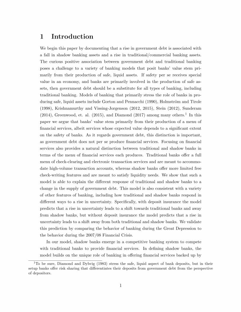
Fig. 1 displays the data on traditional bank size, shadow bank size, and government

debt, all relative to GDP. Table 1 displays results of regressing bank size on the supply

of government debt and real per-capita GDP growth volatility (5-year smoothed). Due

to the trend in MMMF, all regressions involving MMMF include a time trend. The

7

Figure 1: Bank Size and Government Debt

0.2

.4.6

Frac

tion

of G

DP

1980 1990 2000 2010 2020Year

MMMF M2 - Currency - RMFGovt Debt held Domestic

first regression shows results regressing the ratio of traditional bank size to shadow

bank size on government debt and GDP volatility. Here we see very clearly that

a rise in government debt leads to a rise in traditional banking relative to shadow

banking. We also see that a rise in uncertainty as captured in the volatility of GDP

also leads to a substitution towards traditional banking and away from shadow banking.

The second regression shows results of regressing traditional bank size on government

debt and GDP volatility and the third regression shows results of regressing shadow

bank size on government debt and GDP volatility. Government debt enters significant

and positive in the traditional bank regression and significant and negative in the

shadow bank regression, reflecting the complementary nature of government debt and

traditional banking and the substitutability between traditional and shadow banking.

Also, the coefficient on GDP volatility is positive and significant in the traditional

bank regression and negative and significant in the shadow bank regression, reflecting

a flight to quality during times of heightened uncertainty.

3.2 Bank Assets, Financial Crises, and Deposit Insurance

Here we contrast the behavior of shadow and traditional banks with and without

deposit insurance during a financial panic. Historical data on bank trust assets is

obtained from various edition of the Annual Report of the Comptroller of the Currency.

Historical data on M2 and Currency Held by the Public is obtained from Friedman

and Schwartz (1963). For the period 1928 to 1935, Fig. 2 plots for value of M2 net of

8

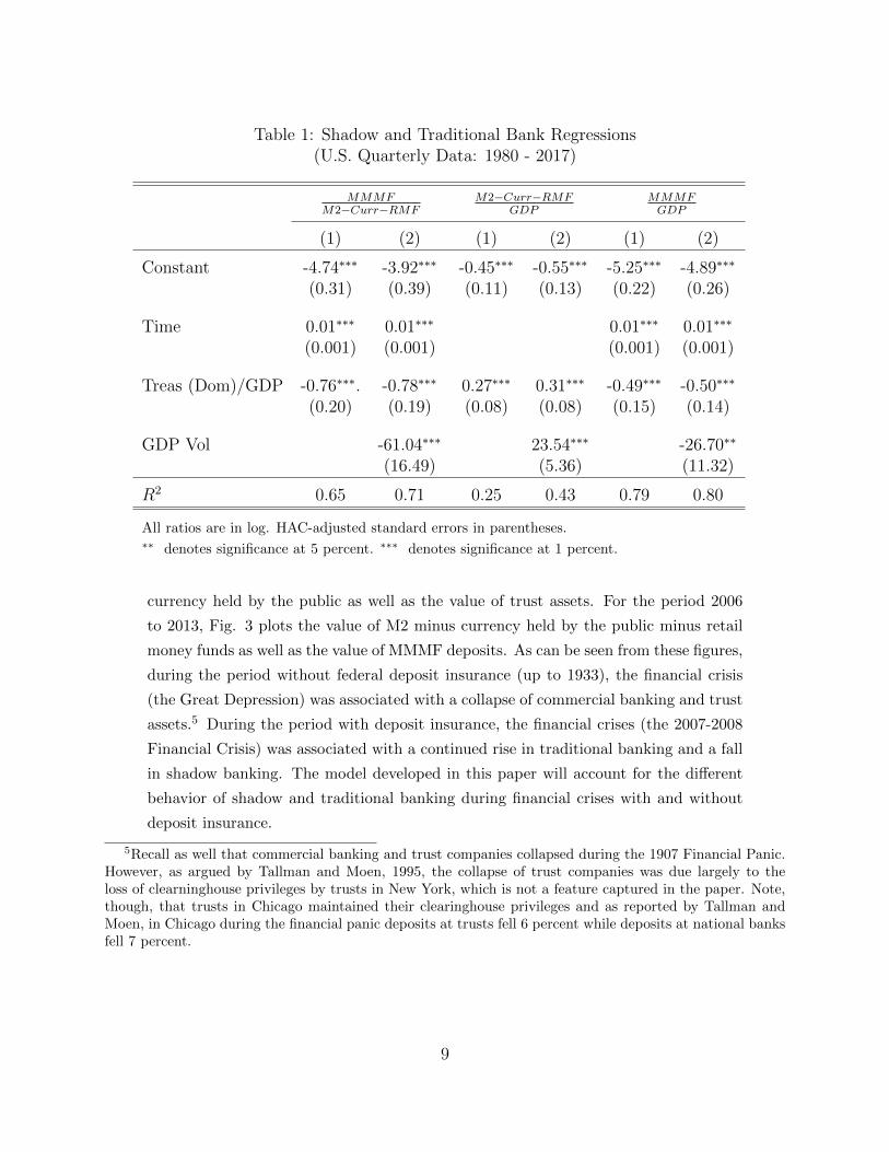
Table 1: Shadow and Traditional Bank Regressions(U.S. Quarterly Data: 1980 - 2017)

MMMFM2−Curr−RMF

M2−Curr−RMFGDP

MMMFGDP

(1) (2) (1) (2) (1) (2)

Constant -4.74∗∗∗ -3.92∗∗∗ -0.45∗∗∗ -0.55∗∗∗ -5.25∗∗∗ -4.89∗∗∗

(0.31) (0.39) (0.11) (0.13) (0.22) (0.26)

Time 0.01∗∗∗ 0.01∗∗∗ 0.01∗∗∗ 0.01∗∗∗

(0.001) (0.001) (0.001) (0.001)

Treas (Dom)/GDP -0.76∗∗∗. -0.78∗∗∗ 0.27∗∗∗ 0.31∗∗∗ -0.49∗∗∗ -0.50∗∗∗

(0.20) (0.19) (0.08) (0.08) (0.15) (0.14)

GDP Vol -61.04∗∗∗ 23.54∗∗∗ -26.70∗∗

(16.49) (5.36) (11.32)

R2 0.65 0.71 0.25 0.43 0.79 0.80

All ratios are in log. HAC-adjusted standard errors in parentheses.∗∗ denotes significance at 5 percent. ∗∗∗ denotes significance at 1 percent.

currency held by the public as well as the value of trust assets. For the period 2006

to 2013, Fig. 3 plots the value of M2 minus currency held by the public minus retail

money funds as well as the value of MMMF deposits. As can be seen from these figures,

during the period without federal deposit insurance (up to 1933), the financial crisis

(the Great Depression) was associated with a collapse of commercial banking and trust

assets.5 During the period with deposit insurance, the financial crises (the 2007-2008

Financial Crisis) was associated with a continued rise in traditional banking and a fall

in shadow banking. The model developed in this paper will account for the different

behavior of shadow and traditional banking during financial crises with and without

deposit insurance.

5Recall as well that commercial banking and trust companies collapsed during the 1907 Financial Panic.However, as argued by Tallman and Moen, 1995, the collapse of trust companies was due largely to theloss of clearninghouse privileges by trusts in New York, which is not a feature captured in the paper. Note,though, that trusts in Chicago maintained their clearinghouse privileges and as reported by Tallman andMoen, in Chicago during the financial panic deposits at trusts fell 6 percent while deposits at national banksfell 7 percent.

9

Figure 2: Bank Assets During the Great Depression

Deposit Insurance

2530

3540

45M

2 - C

urre

ncy,

bil.

1214

1618

Trus

t Ass

ets,

bil.

1928 1930 1932 1934 1936Year

Trust Assets, bil. M2 - Currency, bil.

4 The Model

The model consists of firms, a government, financial intermediaries, and households in

a discrete-time, infinite-horizon, risk-neutral setting subject to uncertainty.

4.1 Firms

A large number of identical firms arise each period and exist for only one period.

Production is an exogenous amount and is fully perishable at the end of the period.

Denote the aggregate output of all firms in the current period by y ≥ 0. Aggregate

output y′ in the next period is drawn from a conditional distribution F (y′, y).

Assumption 1. F (y′, y) > 0 is a distribution function for every y ≥ 0 with compact

support 0 < ymin ≤ y′ ≤ ymax.

As we discuss the equilibrium, we will make further assumptions on F . Denote the

expectation operator over next period’s realizations of y′ conditional on the current

realization y as Ey and denote y = Ey[y′]. Denote also the gross growth rate of

aggregate output by g′ = y′/y.

For simplicity, the only claim on firms is a claim on a portfolio of all firms that

trades one period prior to production. That is, owning z′ claims in the current period

entitles the owner to z′y′ units of aggregate output y′ in the next period. All claims

10

Figure 3: Bank Assets During the 2007/2008 Financial Panic

Lehman bankruptcy

5000

6000

7000

8000

9000

1000

0M

2 - C

urr -

RM

F, b

il.

2000

2500

3000

3500

MM

MF,

bil.

2006 2008 2010 2012 2014Year

MMMF, bil. M2 - Curr - RMF, bil.

are initially owned by households and are traded one period prior to the production of

output. Denote the price of a unit of such a claim in terms of current consumption by

p.

4.2 Government

The government fully honors its existing debt obligations, issues new one-period debt,

and levies a lump-sum tax or pays a lump-sum distribution. Denote the face value in

units of current output of outstanding debt in the current period as B. The government

issues new one-period debt B′ at a per-unit price qb. The difference T = B − qbB′ is

financed by a lump-sum tax (positive or negative) on households. Denote debt per unit

of aggregate output as b′ = B′/y. Assume the government implements a stationary

policy to achieve an amount of debt per unit of aggregate output b′ = G(y) based on

realizations of y.

Assumption 2. G(y) > 0 for every y ≥ 0.

4.3 Financial Intermediaries

Households create and manage financial intermediaries. Financial intermediaries accept

deposits from households and invest in a portfolio of government bonds and equities.

11

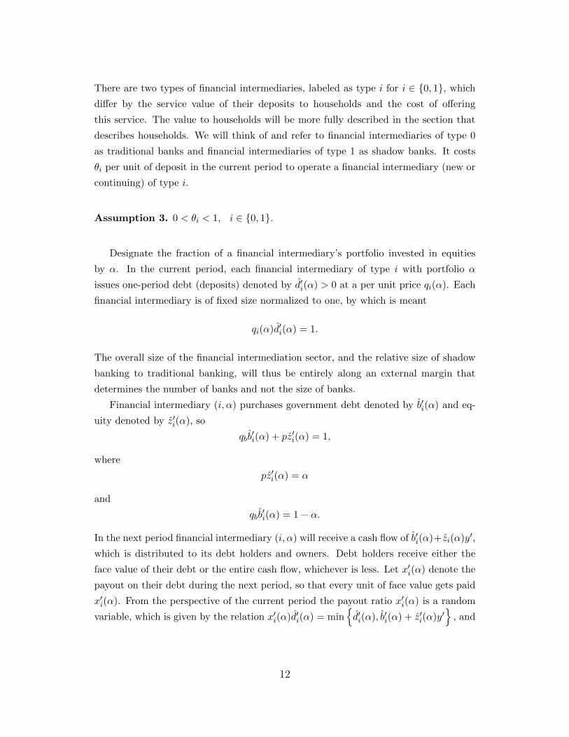
There are two types of financial intermediaries, labeled as type i for i ∈ 0, 1, which

differ by the service value of their deposits to households and the cost of offering

this service. The value to households will be more fully described in the section that

describes households. We will think of and refer to financial intermediaries of type 0

as traditional banks and financial intermediaries of type 1 as shadow banks. It costs

θi per unit of deposit in the current period to operate a financial intermediary (new or

continuing) of type i.

Assumption 3. 0 < θi < 1, i ∈ 0, 1.

Designate the fraction of a financial intermediary’s portfolio invested in equities

by α. In the current period, each financial intermediary of type i with portfolio α

issues one-period debt (deposits) denoted by d′i(α) > 0 at a per unit price qi(α). Each

financial intermediary is of fixed size normalized to one, by which is meant

qi(α)d′i(α) = 1.

The overall size of the financial intermediation sector, and the relative size of shadow

banking to traditional banking, will thus be entirely along an external margin that

determines the number of banks and not the size of banks.

Financial intermediary (i, α) purchases government debt denoted by b′i(α) and eq-

uity denoted by z′i(α), so

qbb′i(α) + pz′i(α) = 1,

where

pz′i(α) = α

and

qbb′i(α) = 1− α.

In the next period financial intermediary (i, α) will receive a cash flow of b′i(α)+zi(α)y′,

which is distributed to its debt holders and owners. Debt holders receive either the

face value of their debt or the entire cash flow, whichever is less. Let x′i(α) denote the

payout on their debt during the next period, so that every unit of face value gets paid

x′i(α). From the perspective of the current period the payout ratio x′i(α) is a random

variable, which is given by the relation x′i(α)d′i(α) = mind′i(α), b′i(α) + z′i(α)y′

, and

12

can be rewritten as

x′i(α) = min

1,

(αy′

p+ (1− α)

1

qb

)qi(α)

.

The next-period payoff to owners of one financial intermediary can similarly be written

as

ω′i(α) = max

0, α

y′

p+ (1− α)

1

qb− 1

qi(α)

.

Households begin a period with Ni(α) financial intermediaries of type i ∈ 0, 1holding portfolio α ∈ [0, 1] for various values of α and choose N ′i(α) financial inter-

mediaries for the current period for various values of α. To clarify with an example,

households may begin a period with N1(α) = 0 except for N1(.5) > 0 and choose

N ′1(α) = 0 except for N ′1(.75) > 0, which means that households begin a period with

all financial intermediaries of type 1 investing 50 percent of their portfolio in equities

and for the next period choose all financial intermediaries of type 1 investing 75 per-

cent of their portfolio in equities. This notation will be suitable for characterizing an

equilibrium in which, for each i, there is an optimal portfolio mix α that all households

choose, but in which this optimal portfolio mix may change over time.

4.4 Households

Risk-neutral households value an infinite sequence of consumption c, c′, c′′, ... via the

expected utility function with constant discount factors

c+ βE[c′] + β2E[c′′] + ... (1)

where 0 < β < 1.

Transactions involving goods cost resources and financial intermediaries offer a ser-

vice that reduces this transaction cost. This service is embodied in the debt or account

d′i, such as various levels of check writing features (e.g., a traditional bank would allow

essentially an unlimited number of checks to be written against the account whereas

a money money mutual fund would allow limited check writing), instant liquidity,

or some accounting/bookkeeping features. To simplify the notation, from the out-

set assume that for each type i financial intermediary, households choose to purchase

debt from one portfolio type α′i, but choose the portfolio type optimally. Later we

will show that households will never have an incentive to deviate from such an equi-

librium (that is, at any point in time there will never be two types of traditional

13

banks or two types of shadow banks, although these types of banks can differ from

each other and over time). Financial services are derived from the CES compos-

ite (Σ1j=0γj(qj(α

′j)d′j(α′j))

ε)1/ε, where qi(α′i)d′i(α′i) for i ∈ 0, 1 is the value of debt

holdings or deposits that a household holds of financial intermediaries of type i with

portfolio α′i (throughout the remainder of this paper, we will simply use Σ to denote

the summation over j from 0 to 1). With this composite, transaction costs are given

by

νc+ψ

η − 1yη(

Σγj(qj(α′j)d′j(α′j))

ε) 1−η

ε,

where ν > 0, ψ > 0, η > 1, ε ≤ 1, γ0 = 1 (a normalization) and y is per-capita firm

output (which is exogenous to household decisions).

Regarding the form of the transaction-cost function, note that a rise in consumption

and liquid assets leads to a less than proportionate rise in transaction costs, reflecting

an economy of scale in transaction costs for wealthier households. Over time the rise

in y will ensure that as consumption and liquid assets rise, transaction costs will rise

in proportion in equilibrium.

A key assumption underlying this model concerns the cost of default of a financial

intermediary for a household. We have in mind that if a financial intermediary is

relied on to provide a service based on a credible promise to maintain the value of

deposits, such as the clearing of checks or providing other forms of liquidity, then

to households there is a cost in addition to the lost value of the defaulted asset if

the financial intermediary is not able to honor its debt (Bansal and Coleman, 1996,

essentially assume this cost is infinite). Specifically, we assume that this additional

cost of default is given by

Σξj(1− xj(αi))dj(αj).

Note that xi(αi) is the payout rate on debt from financial intermediary (i, αi) that

matures in the current period, so (1−xi(αi))di(αi) is the face value of debt that is not

paid. The cost of default is the key mechanism by which the riskiness of an asset limits

its usefulness in providing transaction or liquidity services. While this is an ex-post

feature, certainly ex-ante assets that have a relatively high likelihood of default will

have a lower expected value in terms of financial services. Note that the cost of default

can differ by financial intermediary type, capturing the idea that different levels of

service may be associated with different levels of default cost.

Households own all the financial intermediaries and begin each period directly own-

ing all the firms that yield output in the next period. Denote by zh the amount of

equity directly owned by each household that is a claim to current output (a remaining

14

amount, say zb, is owned by financial intermediaries). Denote by z′ the amount of

equity owned by each household at the beginning of a period that is a claim to next

period’s output (which in aggregate equals one). During the period households sell

claims on firms (to financial intermediaries), keeping equity z′h. Households can also

purchase government debt directly, denoted by b′h, but in doing so do not receive any

financial services (all financial services are provided by financial intermediaries). At

the beginning of each period households also make or receive lump-sum tax payments

to the government, denoted by T . To distinguish between a choice of financial inter-

mediary for deposits (as a consumer of financial services) from one for investment (as

a producer of financial services), let α′i denote a choice of a financial intermediary for

deposits and α′i denote a choice of financial intermediary for investment.

The flow budget constraint for households in the current period is given by

c + νc+ψ

η − 1yη(

Σγj(qj(α′j)d′j(α′i))

ε) 1−η

ε+ Σξj(1− xj(αj))dj(αj) (2)

+ qbb′h + Σqj(α

′j)d′j(α′j) + p(z′h − z′) + Σn′j(α

′j)θj + T

= bh + Σxj(αj)dj(αj) + zhy + Σnj(αj)ωj(αj).

Households must also satisfy various non-negativity conditions, such as n′i ≥ 0, d′i ≥ 0,

b′h ≥ 0 and z′h ≥ 0.

4.5 Equilibrium Conditions

With free entry, if financial intermediary (i, α) is in operation, then owners should

expect discounted profits to equal zero, which leads to the following relation under risk

neutrality

θi = βEy max

0, α

y′

p+ (1− α)

1

qb− 1

qi(α)

.

In general, the value qi(α) is the lowest price a financial intermediary of type i with

portfolio α will accept for its debt. It remains to determine if households will choose

to hold debt from a financial intermediary of type i with portfolio α at the price qi(α).

Households choose state-contingent sequences for c, b′h, d′i, n′i, α

′i, α

′i and z′h to

maximize preferences given by (1), subject to their flow budget constraints given by

(2). Denote the number of next-period financial intermediaries of type i with portfolio

α per unit of aggregate output by n′i(α) = N ′i(α)/y, and denote aggregate financial in-

termediary debt per unit of output by d′i(α) = n′i(α)d′i(α). Denote aggregate household

consumption by c. Denote household aggregate debt holdings by B′h and household

15

aggregate debt holdings per unit of aggregate output by b′h = B′h/y. Note that initial

aggregate household equity holdings equal 1. The first-order conditions, after imposing

market-clearing conditions and transforming to aggregate variables, can be written as:

y = c+ νc+ψ

η − 1

(Σγj(qjd

′j)ε) 1−η

ε y +y

gΣξj(1− xj)dj + yΣn′jθj , (3)

qb ≥ β, w/eq. if b′h > 0, (4)

qi ≥ βEy[x′i] + ψ

(Σγj(qjd

′j)ε) 1−η

ε−1γi(qid

′i)ε−1qi − βξi(1− Ey[x′i]),

w/eq. if d ′i > 0, (5)

qbb′ = qbb

′h + Σ(1− α′j)qjd′j , (6)

p = βy, (7)

qid′i = n′i, (8)

where “w/eq.” denotes “with equality,” where

Ey[x′i] = Ey

[min

1,

(α′iy′

y+ (1− α′i)

β

qb

)qiβ

], (9)

θi = Ey

[max

0, α′i

y′

y+ (1− α′i)

β

qb− β

qi

], (10)

and the non-negativity constraints d′i ≥ 0 and b′h ≥ 0 hold. Further, as shown by

considering deposits at financial intermediaries with alternative strategies for α′i, opti-

mality with respect to α′i requires that

qi ≥ βEy[x′i] + ψ(Σγj(qjd

′j)ε) 1−η

ε−1γi(qid

′i)ε−1qi − βξi(1−Ey[x′i]), for any 0 ≤ α′i ≤ 1,

(11)

for Ey[x′i] and qi defined by

Ey[x′i] = Ey

[min

1,

(α′iy′

y+ (1− α′i)

β

qb

)qiβ

], (12)

θi = Ey

[max

0, α′i

y′

y+ (1− α′i)

β

qb− β

qi

]. (13)

Eq. (3) is the aggregate flow budget constraint. Eq. (4) stipulates that if some

government debt is not held to generate a liquidity value, then its rate of return must

equal the rate of time preference. Eq. (5), the key equation in this model, stipulates

that the return on financial intermediary debt/deposits must reflect both the liquidity

value of this debt as well as the costs of not fulfilling the promise of delivery on any

promised financial service. Eq. (6) accounts for the various holdings of government

16

debt. Eq. (7) relates the price of equity to its expected payoff in a risk-neutral setting.

Eq. (8) relates the number of financial intermediaries (and the total cost of financial

intermediation) to the overall volume of financial intermediation. Eqs. (9)-(10) sum-

marize the expected payout on financial intermediary debt as well as the zero expected

profit condition for financial intermediaries. Conditions (11)-(13) are conditions for

optimality for the type of financial intermediaries and thereby rule out any excess prof-

its for other types of financial intermediaries to enter. To simplify the notation, define

θ = (θ0, θ1), and similarly for ξ, q, d′, n′, and α. For given parameters (θ, ψ, ξ, η),

the system defined by eqs. (3)-(13) determines a recursive, stationary equilibrium

comprised of endogenous variables (c, qb, q, p, d′, n′, α′) conditional on the state y.

To solve for the equilibrium, motivated by eq. (10), for fixed y define H(a, e),

0 ≤ a ≤ 1, 0 < e ≤ 1, such that

0 = Ey

[max

−e, a

(y′

y− 1

)−H(a, e)

]. (14)

Lemma 1: Under Assumptions 1 and 3, a unique function H(a, e) exists such that eq.

(14) holds for every 0 ≤ a ≤ 1, 0 < e ≤ 1. The solution H(a, e) is a continuous function

of a and e. If a ≤ e then H(a, e) = 0, else H(a, e) ≥ 0. If e ≤ e then H(a, e) ≥ H(a, e)

for every 0 ≤ a ≤ 1.

For ease of notation, define hi(a) = H(a, θi). In some sense hi(α′i) is a measure of

the exposure to default of a financial intermediary of type i with investor capital θi

and portfolio α′i, as it is zero when there is no risk of default and positive if there is

risk of default. From the definition of hi and eq. (10) it follows that

α′i + (1− α′i)β

qb− β

qi= θi − hi(α′i). (15)

Combine eqs. (9) and (10) to derive

Ey[x′i] =

(α′i + (1− α′i)

β

qb− θi

)qiβ. (16)

Substitute eqs. (15) and (16) into eq. (5) to derive the following relation that must

hold in equilibrium

(1− α′i)(

1− β

qb

)+ ξihi(α

′i) + θi ≥ ψ

(Σγj(qjd

′j)ε) 1−η

ε−1γi(qid

′i)ε−1, w/eq. if d ′i > 0.

(17)

17

Similarly, the condition of optimality with respect to α′i can be summarized as

(1−α′i)(

1− β

qb

)+ξihi(α

′i)+θi ≥ ψ

(Σγj(qjd

′j)ε) 1−η

ε−1γi(qid

′i)ε−1, for any θi ≤ α′i ≤ 1.

(18)

To summarize, an equilibrium can now be characterized as a (qb, q, b′h, d′, α′) that

solve eqs. (4), (6), (15), (17) and (18), along with (c, n′, p) that solve eqs. (3), (7) and

(8), and in which the non-negativity constraints d′ ≥ 0 and b′h ≥ 0 hold.

The equilibrium can be characterized more sharply by assuming the conditional

distribution F (y′, y) is continuous with density f(y′, y).

Assumption 4.

F (y′, y) is continuous with probability density function f(y′, y) for every y ≥ 0.

Define Ωi(a), a > 0, defined as

Ωi(a) = 1 +hi(a)− θi

a.

In addition to the results of Lemma 1, we can now establish the following properties

of hi.

Lemma 2: Under Assumptions 1-4, the function hi(a) that solves eq. (14) is a twice

continuously-differentiable, concave function with derivatives given by

h′i(a) =

∫∞yΩi(a)

(y′

y − 1)f(y′, y)dy′∫∞

yΩi(a) f(y′, y)dy′≥ 0, (19)

h′′i (a) =

(ah′i(a)− hi(a) + θi

a

)2 f(yΩi(a), y)y

a∫∞yΩi(a) f(y′, y)dy′

≥ 0. (20)

Eq. (18) can now be rewritten using the following Lemma.

Lemma 3: Under Assumptions 1-4, eq. (18) holds if and only if

ξih′i(α′i) ≤ 1− β

qb, w/eq. if α′i < 1. (21)

18

To summarize, an equilibrium is (qb, q, b′h, d′, α′) that solve eqs. (4), (6), (15), (17),

and (21), along with (c, n′, p) that solve eqs. (3), (7) and (8), and in which the non-

negativity constraints d′ ≥ 0 and b′h ≥ 0 hold. It turns out that the existence of an

equilibrium is remarkably easy to prove.

Theorem 4: Under Assumptions 1-4, there exists an equilibrium (qb, q, b′h, d′, α′) that

solves eqs. (4), (6), (15), (17), and (21), along with (c, n′, p) that solves eqs. (3), (7)

and (8), and in which the non-negativity constraints d′ ≥ 0 and b′h ≥ 0 hold.

4.6 Equilibrium for a Simple Example

Suppose aggregate output can take on only two values, 0 with probability 1 − π and

y > 0 with probability π, 0 < π < 1, and that the liquidity aggregate is linear in

traditional and shadow bank deposits, achieved by setting ε = 1. With this two-state

distribution, the function hi is given by

hi(a) = max

0, (a− θi)

1− ππ

. (22)

Note that this discrete distribution violates Assumption 4, hence we need to ensure

eq. (18) holds instead of the condition in Lemma 3. Substitution of eq. (22) into (18)

reveals that

α′i =

θi, if 1−ππ ξi ≥ 1− β

qb.

1, otherwise.(23)

Hence, a financial intermediary either chooses α′i = θi and will thereby be risk-free, or

α′i = 1 and thereby invests all of its assets in equities.

To simplify the exposition, we will make the following additional assumptions for

this example.

Assumption 5.

(i) :γ1

θ1≤ 1

θ0, (24)

(ii) : γ1 < 1, (25)

(iii) :1− ππ

ξ1 < 1 ≤ 1− ππ

ξ0, (26)

(27)

Assumption 5(i) is a key assumption that will lead to traditional banks dominating

19

in the provision of liquidity if they are not constrained by the supply of safe assets.

Assumptions 5(ii) and 5(iii) narrow down the equilibria to one in which traditional

banks always choose to be safe and shadow banks, if they choose to enter and compete

with traditional banks, choose a risky portfolio of assets.

To assist in the characterization of the equilibrium, define the function w = W (D), D >

0 such that

1− (1− θ0)w = ψ

(D

(1− θ0)w

)−η. (28)

Lemma 5: For any D > 0 there exists a unique w that solves eq. (28), 0 < w <

1/(1− θ0), and both W (D) and D/W (D) are increasing functions of D.

Use W to define D∗0 such that

1 = W (D∗0),

and to define D∗1 such that D∗1 = 0 if

ξ1(1− θ1)1− ππ

+ θ1 ≥ γ1,

otherwise D∗1 solves

ξ1(1− θ1)1− ππ

+ θ1 = [(1− θ0)(1−W (D∗1)) + θ0]γ1.

Note that with Lemma 5 and Assumption 5(i) it follows that

0 ≤ D∗1 < D∗0.

Proposition 6: Under Assumptions 1-3 and 5, the equilibrium is comprised of the

following three regions:

20

(Region 1): If βb′ > D∗0, then the equilibrium is given by

α′i = θi, i ∈ 0, 1 (29)

β

qb= 1, (30)

β

qi= 1− θi, i ∈ 0, 1 (31)

q0d′0 =

D∗01− θ0

, (32)

q1d′1 = 0, (33)

qbb′h = βb′ −D∗0. (34)

(Region 2): If D∗1 < βb′ ≤ D∗0, then the equilibrium is given by

α′0 = θ0, (35)

α′1 =

θ1, if 1−ππ ξ1 ≥ 1−W (βb′).

1, otherwise.(36)

β

qb= W (βb′), (37)

β

q0= (1− θ0)W (βb′), (38)

β

q1=

(1− θ1)W (βb′), if 1−ππ ξ1 ≥ 1−W (βb′).

1−θ1π , otherwise.

(39)

q0d′0 =

βb′

(1− θ0)W (βb′), (40)

q1d′1 = 0, (41)

qbb′h = 0. (42)

21

(Region 3): If 0 < βb′ ≤ D∗1, then the equilibrium is given by

α′0 = θ0, (43)

α′1 = 1 (44)

β

qb= W (D∗1), (45)

β

q0= (1− θ0)W (D∗1), (46)

β

q1=

1− θ1

π, (47)

q0d′0 =

βb′

(1− θ0)W (D∗1), (48)

q1d′1 =

1

γ1

D∗1 − βb′

(1− θ0)W (D∗1), (49)

qbb′h = 0. (50)

When there is a large amount of government debt outstanding, specifically βb′ >

D∗0, then the economy is in Region 1, which means that traditional banks completely

crowd out shadow banks. With such high levels of government debt, the price of

government debt does not reflect a liquidity premium. Hence, shadow banks cannot

take advantage of a higher risk-adjusted return from shifting their portfolio to riskier

securities (whose price never reflects a liquidity premium). Traditional and shadow

banks thus compete only on cost θi and return γi characteristics, and by assumption

traditional banks dominate in this comparison in the provision of liquidity.

As the supply of government debt falls, the economy enters Region 2 and then

later Region 3. In Region 2 the price of government debt begins to reflect a liquidity

premium, but still the advantage to shadow banks of shifting their portfolio to riskier

securities does not encourage them to enter. As the economy enters Region 3 the price

of government debt reflects a sufficient premium that both lowers the return on safe

assets held by traditional banks and provides a sufficient advantage to shadow banks

that can absorb the risk of investing in riskier assets, so that shadow banks begin to

enter. In Region 3, a region in which both traditional and shadow banks enter, a rise

in government securities b′ leads to a rise in traditional banking and a fall in shadow

banking. This matches a key feature of the data. In the model, a rise in government

securities leads traditional banks to expand as they earn a higher return on their safe

portfolio and leads shadow banks to contract as they are less able to exploit a liquidity

22

premium by investing in risky securities.

4.7 Some General Results

From eq. (17) it follows that if q0d′0 > 0 and q1d

′1 > 0 (which will occur if ε < 1), then

q1d′1

q0d′0=

γ1

(1− α′0)(

1− βqb

)+ ξ0h0(α′0) + θ0

(1− α′1)(

1− βqb

)+ ξ1h1(α′1) + θ1

1

1−ε

.

This equation captures a number of different features that determine the relative size

of shadow to traditional banking. A higher value of shadow banking as reflected in

γ1 tends to lead to more shadow banking. Similarly, a lower cost of shadow banking

as reflected in a low value of θ1 (or a higher cost of traditional banking as reflected

in a high value of θ0) tends to lead to more shadow banking. Holding government

debt in some sense acts like a tax due to its low return. The total effect of this tax is

captured by the amount of government debt held, 1−α′1 for shadow banks and 1−α′0for traditional banks, times the departure of the return on government debt from its

fundamentals (the rate of time preference), as captured by 1−β/qb. Lastly, the cost of

default times the exposure to default risk, as captured by ξ1h1(α′1) for shadow banks

and ξ0h0(α′0) for traditional banks, determines the relative size of shadow banking.

To further explore the size of shadow to traditional banking, consider two extremes,

one in which government debt is so high that there is no liquidity premium on govern-

ment debt, and one in which no government debt is issued. Suppose also that there is

imperfect substitutability between traditional and shadow bank deposits (ε < 1) and

that there is a continuous distribution of shocks. Define `0 and `1 such that

θi = ψ(Σγj`

εj

) 1−ηε−1γi`

ε−1i , (51)

which means that

`0 =

(θ0

ψ(1 + γ1ϕε)1−ηε−1

)− 1η

, (52)

`1 =

(θ0

ψ(1 + γ1ϕε)1−ηε−1

)− 1η

ϕ, (53)

23

for

ϕ =

(γ1θ0

θ1

) 11−ε

.

Proposition 7: (a) If

βb′ ≥ Σ(1− θj)`j

then the equilibrium is given by

α′i = θi,

qb = β,

β

qi= 1− θi,

qbb′h = βb′ − Σ(1− θj)`j .

qid′i = `i,

(b) If b′ = 0, then the equilibrium is given by

α′i = 1,

β

qi= 1− θi + hi(1),

b′h = 0,

and qid′i for i ∈ 0, 1 solve

ξihi(1) + θi = ψ(Σγj(qjd

′j)ε) 1−η

ε−1γi(qid

′i)ε−1.

From Proposition 7(a) it follows that as qbb′ becomes very large, the size of shadow

banking relative to traditional banking is determined by

q1d′1

q0d′0=

(γ1θ0

θ1

) 11−ε

. (54)

Large values of qbb′ thus do not completely crowd out any particular type of financial

institution, but rather leads the relative size of financial institutions to be determined

by their relative value as reflected in γ1 and relative cost as reflection in θ1/θ0. With

large values of qbb′, shadow banking is relatively larger when it has a higher relative

value (γ1) and a lower relative cost (θ1/θ0). As well, large values of qbb′ make all types

24

of financial institutions safer by raising the return on safe, government assets which in

turn encourages financial intermediaries to invest in these types of safe assets. With

sufficiently large values of qbb′ financial intermediaries invest sufficiently in government

securities so that they become free of default risk.

From Proposition 7(b) it follows that as qbb′ becomes very small, the size of shadow

banking relative to traditional banking is determined by

q1d′1

q0d′0=

(γ1(ξ0h0(1) + θ0)

ξ1h1(1) + θ1

) 11−ε

.

Since both types of financial intermediaries are now exposed to risk of default, the

cost of default as captured by ξ0 and ξ1 is now important in determining their relative

size. Shadow banking is relatively larger when the cost of default of shadow banking

is relatively low (ξ1) or the cost of default of traditional banking is relatively high (ξ0).

Their relative size is also determined by how each type of financial intermediary is

exposed to default risk, as captured by h0(1) and h1(1). A high value of θ0 relative

to θ1 will lead to low value of h0(1) relative to h1(1) as a higher value of θ0 leads to

a larger capital investment in traditional banks that makes them safer for depositors.

Note that these effects tend to work in opposite directions, as a traditional bank may

have a higher value of ξ0, but due potentially to a higher value of θ0, may have a lower

value of h0(1).

In comparing the two extreme cases, (q1b′1)/(q0d

′0) falls as qbb

′ rises from 0 to a very

large value ifξ1h1(1)

ξ0h0(1)<θ1

θ0.

The right side can be thought of as capturing the cost advantage of traditional banking

relative to shadow banking and the left side can be thought of as the risk advantage of

traditional banking relative to shadow banking. If the cost advantage exceeds the risk

advantage, then a rise in government debt will be associated with a rise in traditional

banking relative to shadow banking. The reason is that a rise in government debt

makes risk less important as a feature distinguishing all types of banking. In this range

of parameter values traditional banking has a cost advantage, so as the equilibrium

moves from one where relative size is determined by a risk advantage to one where

relative size is determined by a cost advantage, traditional banking will rise relative

to shadow banking. It is of course not at all clear how this comparison works out in

actual banking environments, as it will depend on values of parameters that need to

be estimated. It is thus not clear that a rise in government debt should be expected to

25

lead to an expansion or contraction of traditional banking relative to shadow banking

in an environment without deposit insurance.

4.8 Simulation: Lognormal Distribution for Output

To study the performance of the model with a continuous distribution for shocks to

aggregate output and for all possible values of government debt, consider simulations

of the model when the log of aggregate output is drawn from a Normal distribution

with mean µ and variance σ2: ln y′ ∼ N (µ, σ2) . Let Φ denote the CDF for N (0, 1) .

Recall the definition of Ωi(α) and note that Ωi(α) solves

Ωi(α) = Ωi(α)Φ

(ln (Ωi(α))

σ+σ

2

)− Φ

(ln (Ωi(α))

σ− σ

2

)+α− θiα

.

The solution Ωi(α) (and thereby hi(α)) will have to be computed numerically, which

will be facilitated by the result that Φ has good approximations that are closed form.

Note as well that

h′i(α) =1

α

θi

1− Φ(

ln Ωi(α)σ + σ

2

)+ Ωi(α)− 1.

We will choose parameter values so that the model matches various moments listed

in Table 2.6 Since this version of the model does not include deposit insurance (deposit

insurance will be included in the next section), the data in Table 2 largely covers the

period 1900 - 1933, which is prior to the Banking Act of 1933 that created federal

deposit insurance. Specifically, we will choose parameters so that the model matches

the conditional variance of log real per-capita GDP, the real return to the stock market,

real interest rates on short-term government debt, commercial paper, and traditional

bank deposits, traditional bank assets as measured by M2 minus currency held by the

public as a ratio to GDP, trust bank assets as a ratio to GDP, as well as the fraction

of asset portfolios that commercial and trust banks invest in government debt or cash.

Note that one moment we will not match is the ratio of government debt to GDP, but

rather by construction we will match the ratio of government debt held by financial

intermediaries to GDP. In the model they are the same (at least for the equilibria in

which government debt offers a liquidity premium), but in reality these two ratios can

be quite different. There are surely a variety of reasons for holding government debt

that are not captured by this model, and here we focus mainly on the demand for

6Due to the difficulty of obtaining historical data, all of the variables do not begin in the same year.

26

government debt by financial intermediaries.

The model is assumed to operate at a quarterly frequency. The variance σ2 of

the conditional distribution of log income y is chosen to match the variance of the

first difference of log per-capita quarterly real GDP, estimated as the annual variance

divided by 4. The subjective discount factor β is chosen to match the real return on

the stock market. The parameter θ0 is chosen so that eq. (15) for i = 0 holds at values

of α0, qb, and q0 from the data, and similarly for θ1. Given θ0, the value of ξ0 is chosen

to be consistent with eq. (21) for i = 0, and similarly for ξ1. Eq. (17) represents two

equations in the remaining four unknown parameters η, ε, ψ, and γ1. Our approach

will be to use eq. (17) to determine ψ and γ1 for various choices of η and ε. In

some sense the more interesting parameter is ε, which determines the substitutability

between traditional and shadow bank deposits, so essentially we will be asking how

the predictions of the model depend on the substitutability between these two types

of assets (we will always assume η = 2). The values of the parameters are in Table 3.

The solution to the model with these parameter values is presented in Table 4. Note

that the solution to the model does not depend on the particular choice of ε, as ψ and

γ1 are chosen to maintain the calibration, but the response of the model to a change

as the quantity of government debt or uncertainty may depend on the value of ε.

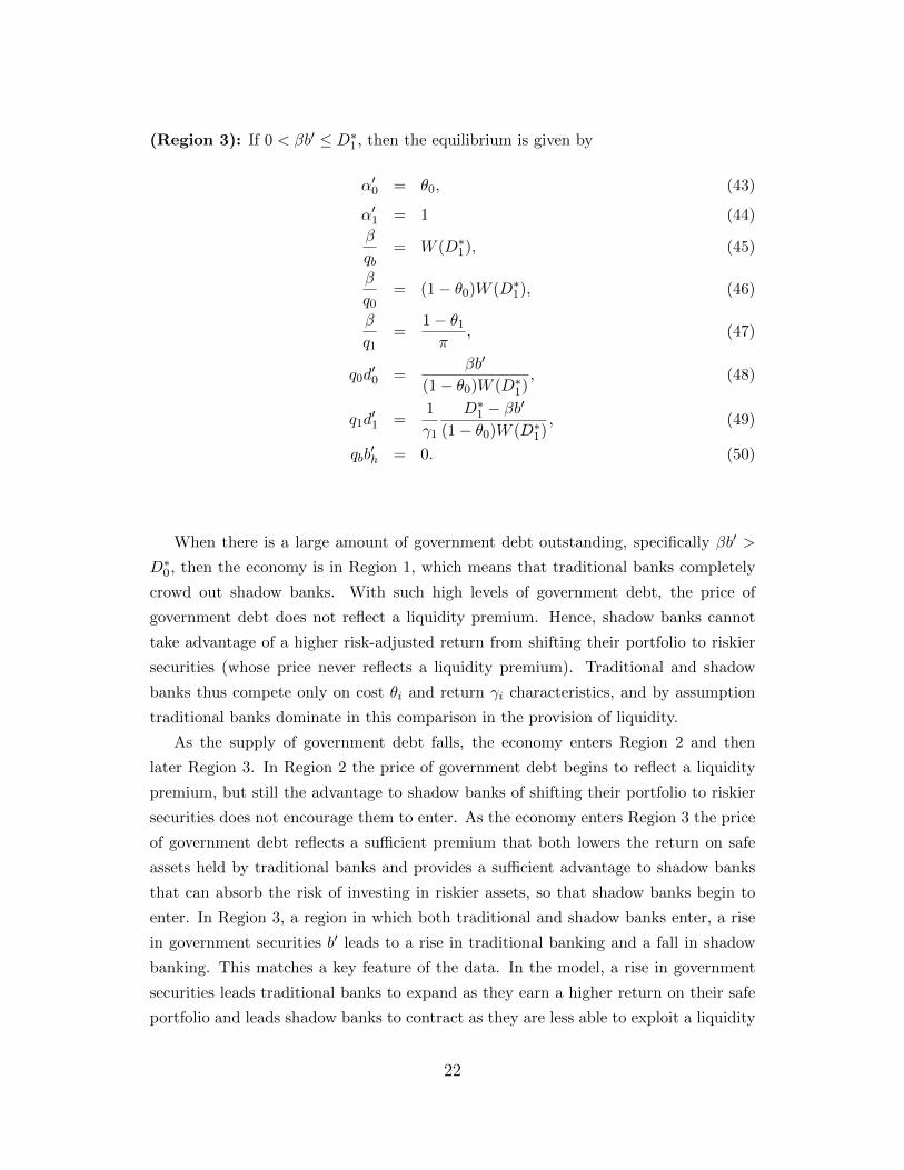
Consider how each type of bank responds to a rise in government debt. Fig. 4 shows

that a rise in government debt leads to a fall in traditional banking and a rise in shadow

banking. The possibility of this result is already explained above. For the parameter

values in Table 3, due to the larger initial capital investment required of a traditional

bank (θ0 > θ1), at low levels of government debt traditional banks have a risk advantage

over shadow banks that is larger than the cost advantage of traditional banks.7 Thus,

traditional banks dominate at low levels of government debt. As government debt

expands, traditional banks lose this advantage and, at the estimated parameter values,

shadow banks offer sufficient value so that they begin to replace traditional banks. As

we will see, though, the situation is very different with deposit insurance.

Fig. 5 documents that the size of traditional and shadow banking both fall with a

rise in uncertainty. Both types of banks choose to be exposed to risk, and the liquidity

value of their deposits depends importantly on the safety of these deposits, so a rise

in uncertainty leads to a fall in the expected value of both types of bank deposits.

This behavior mimics the observed behavior of both types of banks during the Great

7In the simulation h0(1) = 0.0116 and h1(1) = 0.0147, so that (ξ1h1(1))/(ξ0h0(1)) = 1.07 is higher than

θ1/θ0 = .79, which leads to(γ1θ0θ1

) 11−ε

= .91 and(γ1(ξ0h0(1)+θ0)ξ1h1(1)+θ1

) 11−ε

= 0.35.

27

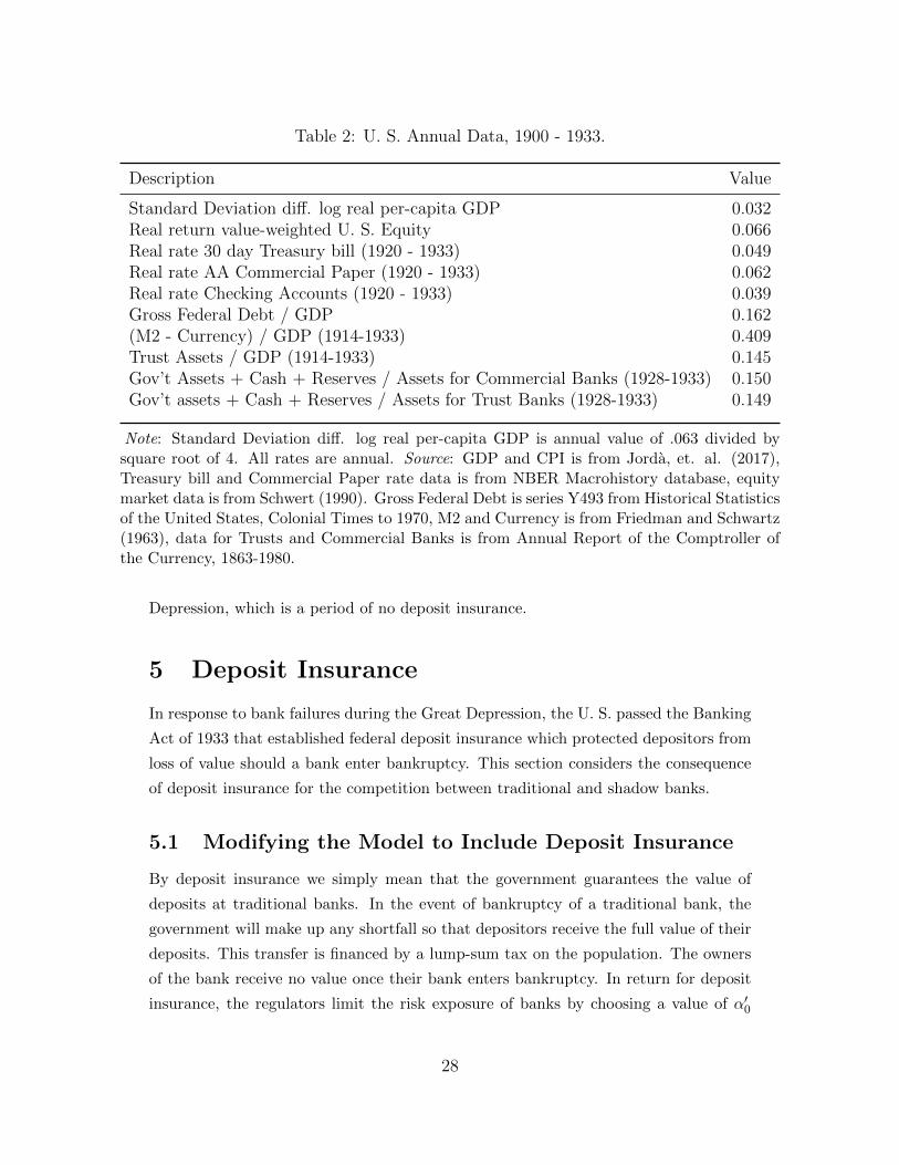
Table 2: U. S. Annual Data, 1900 - 1933.

Description Value

Standard Deviation diff. log real per-capita GDP 0.032Real return value-weighted U. S. Equity 0.066Real rate 30 day Treasury bill (1920 - 1933) 0.049Real rate AA Commercial Paper (1920 - 1933) 0.062Real rate Checking Accounts (1920 - 1933) 0.039Gross Federal Debt / GDP 0.162(M2 - Currency) / GDP (1914-1933) 0.409Trust Assets / GDP (1914-1933) 0.145Gov’t Assets + Cash + Reserves / Assets for Commercial Banks (1928-1933) 0.150Gov’t assets + Cash + Reserves / Assets for Trust Banks (1928-1933) 0.149

Note: Standard Deviation diff. log real per-capita GDP is annual value of .063 divided bysquare root of 4. All rates are annual. Source: GDP and CPI is from Jorda, et. al. (2017),Treasury bill and Commercial Paper rate data is from NBER Macrohistory database, equitymarket data is from Schwert (1990). Gross Federal Debt is series Y493 from Historical Statisticsof the United States, Colonial Times to 1970, M2 and Currency is from Friedman and Schwartz(1963), data for Trusts and Commercial Banks is from Annual Report of the Comptroller ofthe Currency, 1863-1980.

Depression, which is a period of no deposit insurance.

5 Deposit Insurance

In response to bank failures during the Great Depression, the U. S. passed the Banking

Act of 1933 that established federal deposit insurance which protected depositors from

loss of value should a bank enter bankruptcy. This section considers the consequence

of deposit insurance for the competition between traditional and shadow banks.

5.1 Modifying the Model to Include Deposit Insurance

By deposit insurance we simply mean that the government guarantees the value of

deposits at traditional banks. In the event of bankruptcy of a traditional bank, the

government will make up any shortfall so that depositors receive the full value of their

deposits. This transfer is financed by a lump-sum tax on the population. The owners

of the bank receive no value once their bank enters bankruptcy. In return for deposit

insurance, the regulators limit the risk exposure of banks by choosing a value of α′0

28

Table 3: Parameter Values for Model Without Deposit Insurance

ValueParameter Description ε = .85 ε = .90 ε = .95

σ income std. dev. 0.0320 0.0320 0.0320β time discount 0.9841 0.9841 0.9841θ0 unit cost trad. bnk. 0.0140 0.0140 0.0140θ1 unit cost shad. bnk. 0.0110 0.0110 0.0110ξ0 default cost trad. bnk. 0.1884 0.1884 0.1884ξ1 default cost shad. bnk. 0.1588 0.1588 0.1588η transaction cost curv. 2.0 2.0 2.0ψ transaction cost coef. 0.0047 0.0046 0.0046γ1 liq. value shad. bnk. 0.7075 0.7452 0.7849

Table 4: Model Solution Without Deposit Insurance

Variable Description Value

rb interest gov’t debt 0.049r0 interest trad. bnk. 0.039r1 interest shad. bnk. 0.062qbb′ value gov’t debt 0.083

q0d′0 value trad. bnk. 0.400

q1d′1 value shad. bnk. 0.145

qbb′h value gov’t debt holding pvt. 0.0

α′0 frac. equity debt holding trad. bnk. 0.85α′1 frac. equity holding shad. bnk. 0.849

Note: All rates are annualized.

(the fraction of assets invested in risky securities). Since a choice of α′0 limits the risk

exposure of banks, it is meant to capture the effects of both reserve requirements and

capital adequacy requirements. The set-up of the problem is as before, except with

x′0 = 1 (reflecting deposit insurance), and α′0 given by the regulator. The Euler eq. (5)

for i = 0 now becomes

q0 ≥ β + ψ(Σγj(qjd

′j)ε) 1−η

ε−1γ0(q0d

′0)ε−1q0, w/eq. if d ′0 > 0, (55)

29

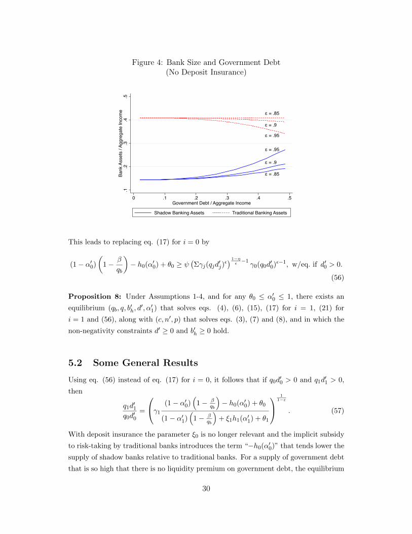
Figure 4: Bank Size and Government Debt(No Deposit Insurance)

ε = .85

ε = .9

ε = .95

ε = .95

ε = .9

ε = .85

.1.2

.3.4

.5Ba

nk A

sset

s / A

ggre

gate

Inco

me

0 .1 .2 .3 .4 .5Government Debt / Aggregate Income

Shadow Banking Assets Traditional Banking Assets

This leads to replacing eq. (17) for i = 0 by

(1− α′0)

(1− β

qb

)− h0(α′0) + θ0 ≥ ψ

(Σγj(qjd

′j)ε) 1−η

ε−1γ0(q0d

′0)ε−1, w/eq. if d ′0 > 0.

(56)

Proposition 8: Under Assumptions 1-4, and for any θ0 ≤ α′0 ≤ 1, there exists an

equilibrium (qb, q, b′h, d′, α′1) that solves eqs. (4), (6), (15), (17) for i = 1, (21) for

i = 1 and (56), along with (c, n′, p) that solves eqs. (3), (7) and (8), and in which the

non-negativity constraints d′ ≥ 0 and b′h ≥ 0 hold.

5.2 Some General Results

Using eq. (56) instead of eq. (17) for i = 0, it follows that if q0d′0 > 0 and q1d

′1 > 0,

then

q1d′1

q0d′0=

γ1

(1− α′0)(

1− βqb

)− h0(α′0) + θ0

(1− α′1)(

1− βqb

)+ ξ1h1(α′1) + θ1

1

1−ε

. (57)

With deposit insurance the parameter ξ0 is no longer relevant and the implicit subsidy

to risk-taking by traditional banks introduces the term “−h0(α′0)” that tends lower the

supply of shadow banks relative to traditional banks. For a supply of government debt

that is so high that there is no liquidity premium on government debt, the equilibrium

30

Figure 5: Bank Size and Uncertainty(No Deposit Insurance)

ε = .95ε = .9

ε = .85

ε = .85

ε = .9ε = .950

.1.2

.3.4

Bank

Ass

ets

/ Agg

rega

te In

com

e

.03 .06 .09 .12 .15sigma

Shadow Banking Assets Traditional Banking Assets

is the same as before since both banks acquire sufficient government debt to become

default free (provided α′0 = θ0). With a fixed value of α′0 > 0 it is no longer possible

to run the thought experiment of letting the supply of government debt go to zero.

However, from eq. (57) we can see that a low required value of α′0 acts like a tax in

forcing traditional banks to hold low interest-bearing government debt, and thus a rise

in the supply of government debt that raises the interest rate may disproportionately

benefit traditional banks.

5.3 Simulation of the Model With Deposit Insurance

We again assume a log-normal distribution of output and calibrate the model in the

similar manner as before, which leads to using the same method for choosing values

of parameters for σ, β, θ0, θ1, ξ1, α0 and α1, except based on data in Table 5 instead

of Table 2. Table 5 is based on more recent data since 1980 that includes deposit

insurance. We will choose parameters to match similar moments as before, although

now traditional bank assets are measured by M2 minus currency held by the public

minus retail money funds, and shadow bank assets are measured by financial assets

held by money market mutual funds. Since depositors never lose any value of their

deposits, the parameter ξ0 is no longer relevant. The only parameters that required a

new method for calibration are ψ and γ1, which are now based on eq. (56) for i = 0

and eq. (17) for i = 1. The new parameter values are listed in Table 6 and the new

31

Table 5: U. S. Quarterly Data, 1980 - 2017.

Description Value

Standard Deviation diff. log real per-capita GDP (1950-2017) 0.009Real return value-weighted CRSP (1950 - 2017) 0.072Real rate 30 day Treasury bill 0.022Real rate AA Commercial Paper 0.029Real rate Checking Accounts (6/2009-4/2018) -0.015Marketable U. S. Treasuries (domestic) / GDP 0.255(M2 - Currency - RMF) / GDP 0.442MMMF / GDP 0.118Treasury bills plus Reserves / Assets for Commercial Banks 0.25Treasury bills / Assets for Shadow Banks 0.10

Note: All rates are annualized based on quarterly data. Source: Equity returnis value-weighted total return from CRSP. All other data is from St. LouisFederal Reserve Bank Fred Database.

model solution is in Table 7. The essential difference is that the calibration leads to

a significantly higher value of ξ1 and a lower value of γ1, which suggests that shadow

banks today offer a different value than shadow banks prior to the Great Depression.

Table 6: Parameter Values for Model With Deposit Insurance

ValueParameter Description ε = .85 ε = .90 ε = .95

σ income std. dev. 0.0090 0.0090 0.0090β time discount 0.9832 0.9832 0.9832θ0 unit cost trad. bnk. 0.0177 0.0177 0.0177θ1 unit cost shad. bnk. 0.0098 0.0098 0.0098ξ1 default cost shad. bnk. 4.8919 4.8919 4.8919η transaction costs curv. 2.0 2.0 2.0ψ transaction cost coef. 0.0057 0.0056 0.0056γ1 liq. value shad. bnk. 0.5335 0.5699 0.6088

Fig. 6 shows that with deposit insurance, a rise in government debt leads to a rise

in traditional bank assets and a fall in shadow bank assets. This is supported in the

data in Table 1 and is explained by the model. Government debt does not directly

offer financial services and hence does not compete with banks in the provision of

financial services. The only effect of changing government debt is thus through directly

32

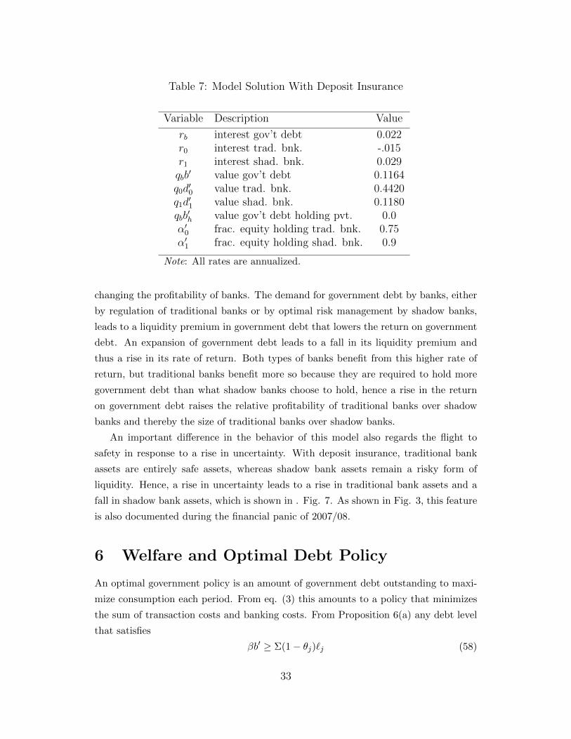
Table 7: Model Solution With Deposit Insurance

Variable Description Value

rb interest gov’t debt 0.022r0 interest trad. bnk. -.015r1 interest shad. bnk. 0.029qbb′ value gov’t debt 0.1164

q0d′0 value trad. bnk. 0.4420

q1d′1 value shad. bnk. 0.1180

qbb′h value gov’t debt holding pvt. 0.0

α′0 frac. equity holding trad. bnk. 0.75α′1 frac. equity holding shad. bnk. 0.9

Note: All rates are annualized.

changing the profitability of banks. The demand for government debt by banks, either

by regulation of traditional banks or by optimal risk management by shadow banks,

leads to a liquidity premium in government debt that lowers the return on government

debt. An expansion of government debt leads to a fall in its liquidity premium and

thus a rise in its rate of return. Both types of banks benefit from this higher rate of

return, but traditional banks benefit more so because they are required to hold more

government debt than what shadow banks choose to hold, hence a rise in the return

on government debt raises the relative profitability of traditional banks over shadow

banks and thereby the size of traditional banks over shadow banks.

An important difference in the behavior of this model also regards the flight to

safety in response to a rise in uncertainty. With deposit insurance, traditional bank

assets are entirely safe assets, whereas shadow bank assets remain a risky form of

liquidity. Hence, a rise in uncertainty leads to a rise in traditional bank assets and a

fall in shadow bank assets, which is shown in . Fig. 7. As shown in Fig. 3, this feature

is also documented during the financial panic of 2007/08.

6 Welfare and Optimal Debt Policy

An optimal government policy is an amount of government debt outstanding to maxi-

mize consumption each period. From eq. (3) this amounts to a policy that minimizes

the sum of transaction costs and banking costs. From Proposition 6(a) any debt level

that satisfies

βb′ ≥ Σ(1− θj)`j (58)

33

Figure 6: Bank Size and Government Debt(Deposit Insurance)

ε = .85

ε = .9ε = .95

ε = .95ε = .9

ε = .85

.1.2

.3.4

.5Ba

nk A

sset

s / A

ggre

gate

Inco

me

.09 .1 .11 .12Government Debt / Aggregate Income

Shadow Banking Assets Traditional Banking Assets

will lead to the term Σξj(1−xj)dj achieving its minimum value of zero. Also according

to Proposition 6(a), as long as debt exceeds the bound in (58) it follows that qid′i = `i.

Since (`0, `1) is also the solution to

min`0,`1

ψ

η − 1

(Σγj`

εj

) 1−ηε + Σ`jθj .

it follows that any value of government debt that exceeds the bound in (58) achieves the

maximum welfare for the model without deposit insurance. Since there is no default

in this equilibrium, along with α′0 = θ0 this is also the optimal government policy with

deposit insurance.

Optimal government policy is thus one with sufficient debt so that interest rates

do not reflect a liquidity premium and all types of banks hold sufficient amount of

government debt to be free of default risk. Both shadow and traditional banks would

thus be free of default risk and would compete solely on value (γ) and cost (θ) consid-

erations. Since both offer a different value/cost bundle and thus offer a value in such

an equilibrium, neither is completely crowded out by the other.

34

Figure 7: Bank Size and Uncertainty(Deposit Insurance)

ε = .85

ε = .9ε = .95

ε = .95ε = .9

ε = .85

0.1

.2.3

.4.5

Bank

Ass

ets

/ Agg

rega

te In

com

e

.007 .008 .009 .01 .011sigma

Shadow Banking Assets Traditional Banking Assets

7 Summary

This paper presents a model in which banks’ value stem from the services they offer.

Safety is an important aspect of banking, but not because banks are unique in offering

safety, but rather that safety is a key dimension of the services they offer. An efficient

payment mechanism, which is the raison d’etre of banking, requires an assurance that

payments will be honored and hence requires that banks are safe institutions. Gov-

ernment debt does not per se produce financial services, and hence does not directly

compete with banks. Rather, banks view government debt as a source of safety and

their demand for these safe assets imparts a liquidity premium to government debt.

The view of banks as offering financial services that rely on safety opens the door

to different types of financial institutions offering different bundles of financial services

and safety. Traditional banks are perhaps more full-service financial institutions that

put a high premium on safety, whereas shadow banks are perhaps more limited-service

financial institutions that put less of a premium on safety. The relationship between

the supply of government debt and the size of traditional and shadow banks is thus

a complex one. Since both value safety, with a sufficient supply of government debt

that eliminates the liquidity premium on government debt, both should hold sufficient

government debt to be free of default risk, and thus the size of traditional versus shadow

banks should be entirely determined by the value and cost of their respective financial

services. With a very limited supply of government debt, the size of traditional versus

35

shadow banks will depend on how each one is able to accommodate a higher exposure

to risk. The parameter values determined in this paper suggests that traditional banks

are better able to accommodate risk, which also implies that a rise in government

debt should lead to a fall in the relative size of traditional to shadow banks. However,

in a world with deposit insurance, the size of traditional banking depends more on

the implicit tax of being required to hold low-interest government debt, so a rise in

government debt and consequent rise in yield on government debt leads to a rise in

traditional banking relative to shadow banking.

An important implication of this paper is that a rise in government debt that

eliminates the liquidity premium on government debt will encourage all financial insti-

tutions, in particular traditional and shadow banks, to hold more government debt and

thereby be less subject to default risk. With the absence of a liquidity premium that

would otherwise hamper the development of either traditional or shadow banks, they

would have to compete based on their fundamental value/cost bundles. It should not

be expected or even desirable that shadow banking vanish due to a rise in the supply of

government debt, as shadow banking may offer a value/cost bundle of services distinct

from traditional banks. A rise in the supply of government debt that eliminated the

liquidity premium would encourage all financial institutions to become safer, thereby

achieving important welfare gains, whatever happens to the relative size of traditional

and shadow banks.

8 Appendix

Proof of Lemma 1: Define Z(a, e, h) = Ey[max−e, a(y′/y − 1) − h]. Note that

Z(a, e, 0) ≥ E[a(y′/y − 1)] = 0, Z(a, e, a(ymax/y − 1)) ≤ 0 since all terms inside the

expectations operator are non-positive, and Z(a, e, h) is a strictly-decreasing function of

h in the range 0 ≤ h ≤ a(ymax/y− 1). There thus exists a unique solution H(a, e) ≥ 0

such that Z(a, e,H(a, e)) = 0. Z(a, e, h) is a continuous function of a, e and h, so

H(a, e) is a continuous function of a and e. For a ≤ e, note that Ey[max−e, ay′/y −a] = E[a(y′/y − 1)] = 0 hence H(a, e) = 0 for a ≤ e. The monotonicity of H with

respect to e follows from the monotonicity of Z with respect to e and h. Q.E.D.

Proof of Lemma 2: The solution hi(a) can be written as

0 = −θiF (yΩi(a), y) +

∫ ∞yΩi(a)

(a

(y′

y− 1

)− hi(a)

)f(y′, y)dy′.

36

The results follow from repeated use of the Fundamental Theorem of Calculus. Note

that h′i(θi) = 0 is well defined, as the left and right limits agree. Q.E.D.

Proof of Lemma 3: Follows from the concavity of the left side of inequality (18)

with respect to α′i. Q.E.D.

Proof of Theorem 4: Define the function T (qb) as

T (qb) = qbb′ − Σ(1− α′j)qjd′j , (59)

where the dependence of α′i on qb is given by eq. (21) and the dependence of qid′i on

qb is given by eq. (17) along with the dependence of α′i on qb just described. Note

that T is a well-defined, continuous function. If T (β) ≥ 0 then the solution is qb = β,

qbb′h = T (β), αi = θi, qi = β/(1 − θi), and qid

′i solves eq. (17) where the left side

equals θi. Suppose T (β) < 0. Note that since θi > 0, it follows that Σ(1 − α′j)qjd′j as

a function of qb is bounded above, hence there exists a q∗b such that T (qb) ≥ 0 for any

qb ≥ q∗b . There thus exists a value of qb between β and q∗b such that T (qb) = 0 . The

associated value of (q, b′h, d′, α′) defines an equilibrium. Q.E.D.

Proof of Lemma 5: These results are straightforward to verify. Q.E.D.

Proof of Proposition 6: (Region 1): Eq. (4) holds since qb = β. Eq. (6) can be

shown to hold just by substitution of the solution into this equation. To show that eq.

(15) holds, note that hi(θi) = 0. Eq. (23) holds since α′i = θi and again since qb = β.

Eq. (17) holds with equality for i = 0 by construction of D∗0, and holds with inequality

for i = 1 as θ1 ≥ θ0γ1 holds by assumption.8

(Region 2): To show that eq. (4) holds, note that W (βb′) ≤ W (D∗0) = 1. Eq. (6)

can again be shown to hold just by substitution of the solution into this equation.

Through straightforward substitution, eq. (15) can be shown to hold for i = 0 and

for i = 1 when 1−ππ ξ1 ≥ 1 −W (βb′). When 1−π

π ξ1 < 1 −W (βb′) use the result that

h1(1) = (1− θ1)1−ππ to show that eq. (15) holds for i = 1. Eq. (17) for i = 0 holds by

definition of W . Eq. (17) for i = 1 and 1−ππ ξ1 ≥ 1−W (βb′) holds if

1− (1− θ1)W (βb′) ≥ (1− (1− θ0)W (βb′))γ1,

which holds since 0 ≤W (βb′) ≤W (D∗0) = 1 and γ1 < 1 and θ1 ≥ θ0γ1 by assumption.

8Equilibria also exist for α′0 < θ0, but all prices and the supply of liquidity are the same for theseequilibria.

37

Eq. (17) for i = 1 and 1−ππ ξ1 < 1−W (βb′) holds if

(1− θ1)ξ11− ππ

+ θ1 ≥ ((1− θ0)(1−W (βb′)) + θ0)γ1,

which holds since in this region W (D∗1) ≤W (βb′) and this inequality holds for W (D∗1)

by construction of D∗1. Eq. (23) holds for i = 0 since 1−ππ ξ0 > 1 by assumption (and

thus 1−ππ ξ0 > 1 − W (βb′)). Eq. (23) holds for i = 1 by construction, given that

βqb

= W (βb′).

(Region 3): Eq. (4) holds since W (D∗1) ≤ 1. Eq. (6) and (15) can be shown to

hold by substitution of the solution into these equations. Eq. (17) for i = 0 holds by

definition of W and eq. (17) for i = 1 holds by construction of D∗1. Eq. (23) holds for

i = 0 for the same reason as in Region 2. Eq. (23) holds for i = 1 if 1−ππ ξ1 ≤ 1−W (D∗1).

From the definition of D∗1, this inequality holds if

1− ππ

ξ1(1− γ1) +

(1− 1− π

πξ1

)(θ1 − θ0γ1) ≥ 0,

which holds since 1−γ1 > 0, θ1−θ0γ1 > 0, and 1− 1−ππ ξ1 > 0 by assumption. Q.E.D.

Proof of Proposition 7: These results are straightforward to verify. Q.E.D.

Proof of Proposition 8: The proof is similar to that of Theorem 4. Q.E.D.

Proof of Proposition 9: These results are straightforward to verify. Q.E.D.

38

9 References

United States, Office of the Comptroller of the Currency, Annual Report of the Comptrollerof the Currency, 1863-1980, https://fraser.stlouisfed.org/title/56, accessed on Septem-ber 18, 2018.

Bansal, Ravi and Wilbur John Coleman II, 1996. “A Monetary Explanation of the EquityPremium, Term Premium, and Risk-Free Rate Puzzles,” Journal of Political Economy104, 1135-1171.

Buchak, Greg, Gregor Matvos, Tomasz Piskorski, and Amir Seru, 2017, “Fintech, Regu-latory Arbitrage, and the Rise of Shadow Banks,” NBER Working Paper 23288.

Chretien, Edouard and Victor Lyonnet, 2018, “Traditional and Shadow Banks,” INSEEWorking Paper.

DeAngelo, Harry and Rene M. Stulz, 2015, “Liquid-claim Production, Risk Management,and Bank Capital Structure: Why High Leverage is Optimal for Banks, Journal ofFinancial Economics, 116, 219-236.

Diamond, Douglas W. and Philip Dybvig, 1983, “Bank Runs, Deposit Insurance, andLiquidity,” Journal of Political Economy, 91(3), 401-419.

Diamond, Douglas W. and Raghuram G. Rajan, 2001, “Liquidity Risk, Liquidity Creation,and Financial Fragility: A Theory of Banking,” Journal of Political Economy, 109(2),287-327.

Diamond, William, 2017, “Safety Transformation and the Structure of the Financial Sys-tem,” Harvard, Working Paper.

Financial Stability Board, 2018, ”Global Shadow Banking Monitoring Report 2017,” avail-able at www.fsb.org/wp-content/uploads/P050318-1.pdf.

Friedman, Milton and Anna Schwartz, 1963, A Monetary History of the United States,1867 - 1960, NBER Publication, Princeton University Press.

Gennaioli, Nicola, Andrei Shleifer, and Robert W. Vishny, 2013, “A Model of ShadowBanking,” Journal of Finance, 68(4), 1331-1363.

Gorton, Gary and George Pennacchi, 1990, “Financial intermediaries and liquidity cre-ation,” Journal of Finance, 45, 49-71.

Gorton, G. and A. Metrick, 2009, “Haircuts,” NBER Working Paper 15273.

Greenwood, Robin, Samuel G. Hanson, and Jeremy C, Stein, 2015, “A Comparative-Advantage Approach to Government Debt Maturity,” Journal of Finance, 70, 1683-1722.

Hanson, Samuel G., Andrei Shleifer, Jeremy C. Stein and Robert W. Vishny, 2015, “Banksas Patient Fixed- Income Investors,” Journal of Financial Economics, 117, 449-469.

39

Historical Statistics of the United States, Colonial Times to 1970, Part 2, 1975, Bureauof the Census.

Holmstrom, Bengt and Jean Tirole, 1998, “Private and Public Supply of Liquidity,” Jour-nal of Political Economy, 106(1), 1-40.

Holmstrom, Bengt and Jean Tirole, 2011, Inside and Outside Liquidity, MIT Press, Cam-bridge, MA.

Jorda, Oscar , Moritz Schularick, and Alan M. Taylor, 2017, “Macrofinancial History andthe New Business Cycle Facts,” in NBER Macroeconomics Annual, 2016, volume 31,edited by Martin Eichenbaum and Jonathan A. Parker. Chicago: University of ChicagoPress.

Krishnamurthy, Arvind and Annette Vissing-Jorgensen, 2012, “The Aggregate Demandfor Treasury Debt,” The Journal of Political Economy, 120, 233-267.

Krishnamurthy, Arvind and Annette Vissing-Jorgensen, 2015, “The Impact of TreasurySupply on Financial Sector Lending and Stability,” Journal of Financial Economics,118, 571-600.

Moen, Jon and Ellis W. Tallman, 1992, “The Bank Panic of 1907: The Role of TrustCompanies,” The Journal of Economic History, 52(3), 611-630.

Moreira, Alan and Alexi Savov, 2017, “The Macroeconomics of Shadow Banking,” TheJournal of Finance, 72(6), 2381-2431.

Nagel, Stefan, 2016, “The Liquidity Premium of Near-Money Assets,” The QuarterlyJournal of Economics. 131(4), 1927-1971.

NBER Macrohistory Database, http://www.nber.org/databases/macrohistory/contents/.

Perotti, Enrico, 2013, “The Roots of Shadow Banking,” CEPR Policy Insight No. 69,December.

Pozsar, Zoltan, Tobias Adrian, Adam Ashcraft and Hayley Boesky, 2013, “Shadow Bank-ing,” Economic Policy Review, 19(2): 1-16.

Schwert, G. William, 1990, ”Indexes of United States Stock Prices from 1802 to 1987,”Journal of Business, 63(3), 399-426

Stein, Jeremy, 2012, “Monetary Policy as Financial Stability Regulation,” Quarterly Jour-nal of Economics, 127, 57-95.

Sunderam, Adi, 2014, “Money Creation and the Shadow Banking System,” Review ofFinancial Studies, 28(4), 939-977.

Tallman, Ellis W. and Jon R. Moen, 1995, “Private Sector Responses to the Panic of 1907:A Comparison of New York and Chicago,” Federal Reserve Bank of Atlanta, EconomicReview, March/April, 1-9.

40