Banking on Deposits:

Maturity Transformation without

Interest Rate Risk

Itamar Drechsler, Alexi Savov, and Philipp Schnabl∗

September 2017

Abstract

We show that in stark contrast to conventional wisdom maturity transformation

does not expose banks to significant interest rate risk. Aggregate net interest margins

have been near-constant from 1955 to 2015, despite substantial maturity mismatch and

wide variation in interest rates. We argue that this is due to banks’ market power in

deposit markets. Market power allows banks to pay deposit rates that are low and

relatively insensitive to interest rate changes, but it also requires them to pay large

operating costs. This makes deposits resemble fixed-rate liabilities. Banks hedge them

by investing in long-term assets whose interest payments are also relatively insensitive

to interest rate changes. Consistent with this view, we find that banks match the

interest rate sensitivities of their expenses and income one for one. This relationship

is robust to instrumenting for expense sensitivity using geographic variation in market

power. Also consistent, we find that banks with lower expense sensitivity hold assets

with substantially longer duration. Our results provide a novel explanation for the

coexistence of deposit-taking and maturity transformation.

JEL: E52, E43, G21, G31Keywords: Banks, maturity transformation, deposits, interest rate risk

∗New York University Stern School of Business, idrechsl@stern.nyu.edu, asavov@stern.nyu.edu, andpschnabl@stern.nyu.edu. Drechsler and Savov are also with NBER, Schnabl is also with NBER and CEPR.We thank Markus Brunnermeier, Eduardo Davila, Mark Flannery, Raj Iyer, Arvind Krishnamurthy, YueranMa, Anthony Saunders, David Scharfstein, Andrei Shleifer, Philip Strahan, Bruce Tuckman, James Vick-ery, and seminar and conference participants at FDIC, Federal Reserve Bank of Philadelphia, LBS SummerSymposium, Office of Financial Research, Princeton University, University of Michigan, and NBER Sum-mer Institute Corporate Finance for their comments. We also thank Patrick Farrell and Manasa Gopal forexcellent research assistance.

I Introduction

A defining function of banks is maturity transformation—borrowing short term and lending

long term. In textbook models, maturity transformation allows banks to earn the average

difference between long- and short-term rates—the term premium—but it also exposes them

to interest rate risk. An unexpected rise in the short-term rate drives up interest expenses

relative to interest income, sinking net interest margins and depleting bank capital. Interest

rate risk is therefore viewed as fundamental to the business of banking, and it underlies the

discussion of how monetary policy impacts the health of the banking system.1

Banks do in fact engage in significant maturity transformation. From 1997 to 2013, the

estimated average duration of aggregate bank assets is 4.3 years versus only 0.4 years for

liabilities. The mismatch of roughly 4 years is large and stable. It implies that a 100-bps

level shock to interest rates would lead to a 100-bps increase in expenses relative to income

for 4 years, and hence a 4 percentage point cumulative reduction in net interest margins.

This represents a big hit to profits for an industry with a 1% return on assets. In present

value terms the shock would induce a 4% decline in assets relative to liabilities, and since

banks are levered ten to one, a 40% decline in bank equity. The shock need not happen all

at once; it can accumulate over time, and is small by historical standards.

Yet, in practice we find that a 100-bps shock to interest rates induces only a 2.4% decline

in bank equity. This is shown in Figure 1, which plots the coefficients from regressions of

industry portfolio returns on changes in the one-year Treasury rate around Federal Open

Market Committee (FOMC) meetings.2 In addition to being relatively small, the coefficient

for banks (−2.42) is also very similar to that for the overall market portfolio (−2.26) and is

close to the median among the 49 industries. Thus, banks are no more exposed to interest

rate shocks than the typical nonfinancial firm.

1In 2010, Federal Reserve Vice Chairman Donald Kohn argued that “Intermediaries need to be sure thatas the economy recovers, they aren’t also hit by the interest rate risk that often accompanies this sort ofmismatch in asset and liability maturities” (Kohn 2010).

2We use the value-weighted Fama-French 49 industry portfolios, available on Ken French’s website. Weuse a two-day-window around FOMC meetings as in Hanson and Stein (2015). The sample is from 1994(when the FOMC began making announcements) to 2008 (when the zero lower bound was reached). Wefocus on the 113 scheduled meetings over this period (the 5 unscheduled ones are contaminated by othertypes of interventions). The results are unaffected if we use other maturities, or if we identify a level shift inthe yield curve by controlling for slope changes.

1

To understand this low exposure, we analyze bank cash flows. We show that, in stark

contrast to the textbook view, they are insensitive to interest rate changes. Panel A of

Figure 2 plots banks’ aggregate net interest margin (NIM), which is the difference between

interest income and expenses as a percentage of assets. NIM is a standard measure of bank

profitability that captures the impact of interest rates on bank cash flows. From 1955 to

2015, aggregate NIM stayed in a narrow band between 2.2% and 3.7% even as the short-term

interest rate (the Fed funds rate) fluctuated between 0% and 16%. Moreover, movements

in NIM within this band have been very slow and gradual: yearly NIM changes have a

standard deviation of just 0.13% and zero correlation with the Fed funds rate. This lack of

sensitivity flows through to banks’ bottom line: return on assets (ROA) displays virtually

no relationship with interest rate fluctuations.

We show that bank cash flows have no exposure to interest rates because banks closely

match the interest rate sensitivity of their income and expenses. This is shown at the

aggregate level in Panel B of Figure 2. Interest income has a low sensitivity to the short

rate. This is expected since banks’ assets are primarily fixed-rate and long-term. What is

surprising is that banks are able to match this low sensitivity on the expense side despite

having liabilities that are overwhelmingly of zero or near-zero maturity. This is due to banks’

market power in retail deposit markets (Drechsler, Savov, and Schnabl 2017), which allows

them to keep deposit rates low even as market rates rise. Since retail (core) deposits are

over 70% of bank liabilities, the overall sensitivity of banks’ interest expenses is low. Market

power thus allows banks to simultaneously maintain a large maturity mismatch and yet a

near-perfect match in the interest sensitivities of their income and expenses, i.e. to engage

in maturity transformation without interest rate risk.

In fact, banks not only can but must engage in maturity transformation in order to avoid

interest rate risk. Since their expenses are insensitive, holding only short-term assets would

expose banks to the risk of a decline in interest rates. Such a decline would cause interest

income to fall relative to expenses, making banks unable to cover the large operating costs

(salaries, branches, marketing) associated with running a deposit franchise and obtaining

market power. These costs are reflected (net of fee income) in the sizable 2% to 3% gap

between NIM and ROA in Panel A of Figure 2. To hedge these costs against a drop in

2

interest rates, banks must hold sufficient long-term fixed-rate assets.

These facts add up to a simple view of banks’ business model. It is built on a foundation

of core deposits, which give banks stable and predictable expenses and allow them to invest

in long-term assets.3 This generates a NIM of about 3%, out of which banks pay 2% in net

operating costs to maintain their deposit base. This leaves a 1% ROA, which banks lever

up ten to one into a 10% return on equity (ROE). Market power in deposit markets keeps

these numbers steady year in and year out, making this business model viable.

We present a simple model that captures this view. In the model, banks pay a fixed

operating cost each period to maintain a deposit franchise. This gives them market power

and allows them to pay a deposit rate that is only a fraction of the economy’s short-term

rate as in Drechsler, Savov, and Schnabl (2017). As a result, their expenses are relatively

insensitive to interest rates. To hedge them, banks invest in assets with relatively insensitive

income streams, i.e. long-term fixed-rate assets. Under free entry (zero ex ante deposit

rents), banks exactly match the sensitivities of their interest income and expenses. The

model thus explains the sensitivity matching of aggregate interest income and expenses and

the stability of NIM and ROA in Figure 2. The model further implies that these results

should hold bank by bank. We test this prediction in the cross section.

We do so using quarterly Call Report data on all U.S. commercial banks from 1984 to

2013.4 We estimate each bank’s interest expense sensitivity by regressing the change in its

interest expense rate (interest expense divided by assets) on contemporaneous and lagged

changes in the Fed funds rate. We then sum the coefficients to obtain a bank-level estimated

sensitivity, which we call the interest expense beta. We compute an interest income beta for

each bank analogously. The average expense beta (0.360) and average income beta (0.379)

are very similar. They show that the rates banks pay and earn on average rise by just over

a third of the rise in the Fed funds rate. At the same time, there is substantial variation in

expense and income betas across banks in the 0.1 to 0.6 range.

We find that our expense and income beta estimates line up strongly across banks. The

raw correlations are 51% among all banks and 58% among the largest 5% of banks. The

3Hanson, Shleifer, Stein, and Vishny (2015) put forward a related view based on the stability of depositswith respect to liquidity (run) risk. We think of these as working in tandem.

4We have posted the code for creating our sample and the sample itself on our websites.

3

corresponding slopes from a univariate regression of income betas on expense betas are

0.768 and 0.878. The high correlations and slope coefficients close to one show that there is

strong matching, as predicted by the model. These results are confirmed in two-stage panel

regressions with time fixed effects, which give estimates that are more precise and for large

banks closer to one (0.765 for all banks, 1.114 for the top 5%). The strong matching leaves

banks’ profitability largely unexposed: ROA betas (computed in the same way as expense

betas) are close to zero across the distribution of banks. Banks are thus able to engage in

maturity transformation without exposing their bottom line to significant interest rate risk.

Our results predict that a bank with an expense beta of one would have an income beta

close to one. While these betas are outside the range of our sample, they have predictive

power out of sample. In particular, they accurately describe money market funds, which

obtain funding at the Fed funds rate and hold only short-term assets, i.e. they do not

engage in maturity transformation.

The insensitivity of banks’ profits to interest rate shocks is confirmed when we look at

the reactions of their stock prices. Following the methodology behind Figure 1, we construct

“FOMC betas” for all publicly traded commercial banks. As in Figure 1, the average FOMC

beta is similar to that of the overall market. Across banks, FOMC betas are flat in both

expense and income betas. The latter result in particular shows that the share of long-term

assets on a bank’s balance sheet, as reflected in its income beta, is unrelated to the interest

rate exposure of its stock price. This is explained by the high degree of sensitivity matching

between assets and liabilities.

Our model predicts that banks with lower expense betas should have lower income betas

and thus hold more long-term fixed-rate assets. We test this prediction using an estimate

of asset duration available from the Call Reports after 1997. The estimate is repricing ma-

turity, which is defined as the time until an asset’s interest rate resets.5 We find a strong

negative relationship between estimated duration and interest expense betas. The regression

coefficient is −3.951 years, and is robust to a number of controls (wholesale funding, capi-

talization, size). The magnitude is similar to the average duration of bank assets and again

5Note that repricing maturity contrasts with remaining maturity, which is the time until the asset termi-nates. An example illustrating the important difference is a floating rate bond whose repricing maturity isone quarter even as its remaining maturity can be many years.

4

extrapolates to fit the duration of money market funds.

We consider alternative explanations for our matching results. One possibility is that

banks with higher expense betas face more run (liquidity) risk, which leads them to hold

more short-term assets as a buffer. Although this explanation does not predict one-to-

one matching, it goes qualitatively in the same direction. We address it by looking at

the composition of banks’ balance sheets, specifically at the shares of loans versus securities.

Because loans are much less liquid than securities, the liquidity risk explanation predicts that

high expense-beta banks hold fewer loans and more securities. We find the exact opposite:

low expense-beta banks hold fewer loans and more securities. This finding fits our model

because securities have substantially higher average duration (8.8 years versus 3.8 years for

loans). Liquidity risk is thus unlikely to explain our results.6

We also consider the possibility that the sensitivity matching is the product of market

segmentation. Perhaps banks with more market power over deposits also have more long-

term lending opportunities. This explanation also does not predict one-to-one matching.

Nevertheless, we test it by examining whether banks match the interest income betas of

their securities holdings to their interest expense betas. Since securities are bought and

sold in open markets, they are immune to market segmentation. We once again find close

matching, even when we focus narrowly on banks’ holdings of Treasuries and agency MBS.

This shows that banks actively match their interest income and expense sensitivities.

Finally, we provide direct evidence for the market power mechanism underlying our

model by exploiting three sources of geographic variation in market power. The first is

local market concentration. We find that banks that raise deposits in more concentrated

markets have lower expense betas and lower income betas, and that the coefficient for the

matching relationship is again close to one. Thus banks match variation in expense betas

that is due to market power, as predicted by our model.

For the second source of variation we use branch-level data on retail deposit products

(interest checking, savings, and small time deposits) from the data provider Ratewatch.

6In addition to loans and securities, a small fraction of banks (about 8%) make use of interest ratederivatives. In principle, banks can use these derivatives to hedge the interest rate exposure of their assets,yet the literature has shown that they actually use them to increase it (Begenau, Piazzesi, and Schneider2015). We show that our sensitivity matching results hold both for banks that do and do not use interestrate derivatives. Hence, derivatives use does not drive our results.

5

These deposits are marketed directly to households in local markets and are thus the source

of banks’ market power. They are also well below the deposit insurance limit and hence

immune to credit and run risk. We regress the average rates paid on these retail deposits

in each county on Fed funds rate changes to obtain a county-level retail deposit beta. We

then take a weighted average of these county betas to obtain a retail deposit beta for each

bank, using the shares of the bank’s branches in each county as weights. We show that

banks’ retail deposit betas are strongly related to their overall expense betas. Moreover,

banks again match their income betas one for one to the differences in overall expense betas

induced by variation in retail deposit betas.

For the third source of variation, we take this approach one step further and add bank-

time fixed effects in the estimation of the county-level retail deposit betas. Thus, the resulting

betas are identified only from differences in retail deposit rates across branches of the same

bank. This purges the betas of any time-varying bank characteristics (e.g., loan demand),

giving us a clean measure of local market power. Using the purged betas as an instrument

for banks’ overall expense betas, we once again find one-for-one matching between income

and expense sensitivities.

The rest of this paper is organized as follows. Section II discusses the related literature;

Section III presents the model; Section IV discusses the data; Section V presents our main

results on matching; Section VI looks at the asset side of bank balance sheets; Section VII

shows our results on market power; and Section VIII concludes.

II Related literature

Banks issue short-term deposits and make long-term loans. This dual function underlies

modern banking theory (Diamond and Dybvig 1983, Diamond 1984, Gorton and Pennacchi

1990, Calomiris and Kahn 1991, Diamond and Rajan 2001, Kashyap, Rajan, and Stein 2002,

Hanson, Shleifer, Stein, and Vishny 2015). Central to this literature is the liquidity risk

inherent in issuing runnable deposits.7 Our paper focuses on the interest rate risk inherent

7For measures of liquidity risk in the banking sector, see Brunnermeier, Gorton, and Krishnamurthy(2012) and Bai, Krishnamurthy, and Weymuller (2016).

6

in issuing deposits while engaging in maturity transformation. We argue that market power

in deposit markets lowers the interest rate sensitivity of banks’ expenses, making them

resemble fixed-rate liabilities. As a consequence, banks hold long-term assets so that they

face minimal net interest rate exposure. This explains how the banking sector has achieved

stable profitability in the face of wide fluctuations in interest rates over the past sixty years.

An important distinction of our explanation for banks’ maturity transformation is that

it does not rely on the presence of a term premium. In Diamond and Dybvig (1983), a term

premium is induced by household demand for short-term claims. In a recent class of dynamic

general equilibrium models, maturity transformation varies with the magnitude of the term

premium and banks’ effective risk aversion (He and Krishnamurthy 2013, Brunnermeier and

Sannikov 2014, 2016, Drechsler, Savov, and Schnabl 2015). In Di Tella and Kurlat (2017),

as in our paper, deposit rates are relatively insensitive interest rate changes (due to capital

constraints instead of market power). This makes banks less averse to interest rate risk than

other agents and induces them to maintain a maturity mismatch in order to earn the term

premium.8 In contrast, our paper focuses on risk management rather than risk taking. While

both risk taking and risk management are consistent with some maturity transformation,

only the risk-management explanation gives the strong quantitative prediction of one-to-one

matching between between banks’ interest income and expense sensitivities.9

Another important distinction is that our explanation implies that banks are relatively

insulated from the balance sheet channel of monetary policy (Bernanke and Gertler 1995),

which works through the influence of interest rate changes on bank net worth. It also

addresses the concern that maturity transformation leads to financial instability (Kohn 2010).

The risk of instability is sometimes invoked as an argument for narrow banking (the idea that

banks should hold only short-term safe assets, see Pennacchi 2012). Our analysis suggests

8The Treasury term premium has declined and appears to have turned negative in recent years (seehttps://www.newyorkfed.org/research/data indicators/term premia.html). At the same time, banks’ matu-rity mismatch has remained stable or actually increased.

9Consistent with the risk management view, Bank of America’s (2016) annual report reads, “Our overallgoal is to manage interest rate risk so that movements in interest rates do not significantly adversely af-fect earnings and capital.” Accordingly, in 2016 each of the top four U.S. banks reported in their annualreport that a parallel upward shift in interest rates would exert a modest positive influence on net interestincome. For formal models of bank risk management, see Froot, Scharfstein, and Stein (1994) and Nageland Purnanandam (2015).

7

that narrow banking could actually make banks more unstable.

The empirical literature looks at banks’ exposure to interest rate risk. In a small sample

of fifteen banks, Flannery (1981) finds that bank profits have a surprisingly low exposure

and frames this as a puzzle. Flannery and James (1984a) and English, den Heuvel, and

Zakrajsek (2012) examine the cross section of banks’ stock price exposures, but without

comparing banks to the broader market as we do in Figure 1.10

One possibility is that banks use derivatives to hedge their interest rate risk exposure

(see, e.g. Freixas and Rochet 2008). Under this view they are not really engaging in maturity

transformation but rather transferring it to the balance sheets of their derivatives counter-

parties. Yet as Purnanandam (2007), Begenau, Piazzesi, and Schneider (2015) and Rampini,

Viswanathan, and Vuillemey (2016) show, derivatives use is limited and may actually am-

plify banks’ maturity mismatch. This is consistent with our explanation where banks have

a maturity mismatch but are nevertheless hedged against interest rates.

As Drechsler, Savov, and Schnabl (2017) show, banks with insensitive deposit rates expe-

rience greater deposit outflows when interest rate go up (this is consistent with their higher

market power). This causes their balance sheets to contract even though NIM remains the

same. Combined with the results in this paper, this can shed light on why banks with a big-

ger income gap (a measure of maturity mismatch) contract lending more following interest

rate increases (Gomez, Landier, Sraer, and Thesmar 2016).

A canonical example of interest rate risk in the financial sector comes from the Savings

and Loans (S&L) crisis of the 1980s. An unprecedented rise in interest rates inflicted sig-

nificant losses on these institutions, which were subsequently compounded by risk shifting

(White 1991). We draw two lessons from this episode. Remarkably, unlike the S&L sector,

the commercial banking sector saw no decline in NIM during this period (see Figure 2).

Moreover, as White (1991) points out, the rise in interest rates happened to occur right after

deposit rates were deregulated, making it difficult for S&Ls to anticipate the effect of such a

large shock on their funding costs. Thus, when it comes to banks’ interest rate risk exposure

the S&L crisis is in some ways the exception that proves the rule.

10The exposures in English, den Heuvel, and Zakrajsek (2012) are somewhat larger than ours becausetheir sample includes unscheduled FOMC meetings. Nevertheless, they remain much smaller than expectedand only slightly larger than the exposure of the whole market (see Bernanke and Kuttner 2005, Table III).

8

The deposits literature has documented the low sensitivity of deposit rates to market

rates, a key ingredient of our paper (Hannan and Berger 1991, Neumark and Sharpe 1992,

Driscoll and Judson 2013, Yankov 2014, Drechsler, Savov, and Schnabl 2017). A subset of this

literature (Flannery and James 1984b, Hutchison and Pennacchi 1996) estimates the effective

duration of deposits, finding it to be higher than their contractual maturity, consistent with a

low interest rate sensitivity.11 Nagel (2016) and Duffie and Krishnamurthy (2016) extend the

low sensitivity finding to a wider set of bank instruments. Brunnermeier and Koby (2016)

argue that deposit rates become fully insensitive when nominal rates turn negative, and that

this impacts bank profitability and undermines the effectiveness of monetary policy.

The deposits literature has also examined the relationship between deposit funding and

bank assets. Kashyap, Rajan, and Stein (2002) emphasize the synergies between the liq-

uidity needs of depositors and bank borrowers. Gatev and Strahan (2006) show that banks

experience inflows of deposits in times of stress, which in turn allows them to provide more

liquidity to their borrowers. Hanson, Shleifer, Stein, and Vishny (2015) argue that banks

are better suited to holding fixed-rate assets than shadow banks because deposits are more

stable than shadow bank funding. Berlin and Mester (1999) show that deposits allow banks

to smooth out aggregate credit risk. Kirti (2017) finds that banks with more floating-rate

liabilities extend more floating-rate loans to firms. Our paper focuses on banks’ exposure

to interest rate risk and provides an explanation for the co-existence of deposit-taking and

maturity transformation.

III Model

We provide a simple model of a bank’s investment problem to explain our aggregate findings

and obtain cross-sectional predictions. Time is discrete and the horizon is infinite. The bank

funds itself by issuing risk-free deposits. Its problem is to invest in assets so as to maximize

the present value of its future profits, subject to the requirement that it remain solvent so

that its deposits are indeed risk free. For simplicity we assume the bank does not issue any

11These papers focus on the contribution of deposit rents to bank valuations. A recent paper in this areais Egan, Lewellen, and Sunderam (2016), which finds that deposits are the main driver of bank value.

9

equity. Though it is straightforward to incorporate equity, the bank is able to avoid losses

and therefore does not need to issue equity.

To raise deposits the bank operates a deposit franchise at a cost of c per deposit dollar.

This cost is due to the investment the bank has to make in branches, salaries, advertising,

and so on to attract and service its deposit customers. Importantly, the deposit franchise

gives the bank market power, which allows it to pay a deposit rate of only

βExpft, (1)

where 0 < βExp < 1 and ft is the economy’s short rate process (i.e. the Fed funds rate).

Drechsler, Savov, and Schnabl (2017) construct a model that micro-founds this deposit rate

as an industry equilibrium among banks with deposit market power. A bank with high

market power has a low value of βExp, while a bank with low market power, such as one

funded mostly by wholesale deposits, has a βExp close to one. Note that deposits are short

term. While adding long-term liabilities to the model is straightforward, they would not

change the mechanism and hence we leave them out. Moreover, as documented above,

banks’ liabilities are largely short term.

On the asset side, we assume that markets are complete and prices are determined by the

stochastic discount factor mt. Like all investors, banks use this stochastic discount factor

when valuing profits.12 Their problem is thus

V0 = maxINCt

E0

[∞∑t=0

mt

m0

(INCt − βExpft − c

)](2)

s.t. E0

[∑∞t=0

mt

m0INCt

]= 1 (3)

and INCt ≥ βExpft + c (4)

where INCt is the time and state contingent income stream generated by the bank’s asset

portfolio. Note that we normalize the bank’s problem to one dollar of deposits, which is

without loss of generality since the problem scales linearly in deposit dollars. Equation (3)

12This is a basic distinction between our framework and the literature which typically models banks asseparate agents with distinct risk preferences or beliefs.

10

gives the budget constraint: the present value of future income must equal its current value

of one dollar. Equation (4) is the solvency constraint: the bank’s income must always exceed

its interest expenses βExpft and operating costs c.

The bank faces two solvency risks. The first is that its interest expenses rise with the

short rate (βExp > 0), so it must ensure that its income stream is also sufficiently positively

exposed to ft. Otherwise it will become insolvent when ft is high. This means that a

sufficient fraction of the bank’s portfolio must resemble short-term bonds, whose interest

payments rise with the short rate. This condition echoes the standard concern that banks

should not be overly maturity-mismatched, i.e., that a large-enough fraction of their assets

should be short term. Yet, there is an important difference. The standard concern is based

on the short maturity of deposits, because this suggests a high sensitivity to the short rate.

However, due to market power the bank’s deposit sensitivity βExp can be well below one, in

which case so can its portfolio share of short-term assets.

The second solvency risk the bank faces is due to its operating costs c, which are insen-

sitive to the short rate. As a consequence, the bank’s income must be insensitive enough so

that it can cover these operating costs in case ft is low. Thus, the bank must hold sufficient

long-term fixed-rate assets, which produce an income stream that is insensitive to the short

rate. Put another way, when ft is low the bank’s deposit franchise generates only small

interest savings, yet continues to incur the same level of operating costs. To hedge against

this low-rate scenario, the bank must hold sufficient long-term assets.

These conditions pin down the bank’s portfolio when it makes no excess rents, as is the

case under free ex ante entry into the banking industry. We obtain the following.

Proposition 1. Under ex ante free entry, V0 = 0, and the bank’s income stream is given by:

INCt = βExpft + c. (5)

Hence the bank matches the interest sensitivities of its income and expenses:

Income beta ≡ βInc =∂INCt∂ft

= βExp ≡ Expense beta. (6)

11

When there are no excess rents, the present value of the interest savings generated by

the deposit franchise is equal to the present value of its operating costs.13 The bank must

therefore apply its whole income stream to satisfying the solvency constraint, leading to the

simple prediction that the bank matches the interest sensitivities of its income and expenses.

We test this prediction in the following sections by analyzing the cross section of banks.

Finally, although we allow asset markets to be complete, it is actually simple for the

bank to implement equation (5) using standard assets. It can do so by investing βExp share

of its assets in short-term bonds, and the remainder in long-term fixed-rate bonds. We use

this observation to provide additional empirical tests of our model.

IV Data

Bank data. Our bank data is from the U.S. Call Reports provided by Wharton Research Data

Services. We use data from January 1984 to December 2013. The data contain quarterly

observations of the income statements and balance sheets of all U.S. commercial banks. The

data contain bank-level identifiers that can be used to link to other datasets.

In part of the analysis, we use repricing maturity as a proxy for duration. The repricing

maturity of an asset is the time until its rate resets or the asset terminates, whichever comes

sooner. For instance, the repricing maturity of a floating-rate bond is one quarter, while the

repricing maturity of a fixed-rate bond is its terminal maturity.

To calculate the repricing maturity of bank assets and liabilities, we follow the method-

ology in English, den Heuvel, and Zakrajsek (2012). Starting in 1997, banks report their

holdings of five asset categories (residential mortgage loans, all other loans, Treasuries and

agency debt, MBS secured by residential mortgages, and other MBS) broken down into six

bins by repricing maturity interval (0 to 3 months, 3 to 12 months, 1 to 3 years, 3 to 5 years,

5 to 15 years, and over 15 years). To calculate the overall repricing maturity of a given asset

category, we assign the interval midpoint to each bin (and 20 years to the last bin) and take

13Formally, the condition is (1− βExp) = c×E0

[∑∞t=0

mt

m0

]= c×Pconsol, where Pconsol is the price of a 1

dollar consol bond. (1−βExp) is the present value of the interest savings generated by the deposit franchise,while c×Pconsol is the present value of the perpetuity of operating costs c. Thus, under ex ante free entry alower expense beta βExp implies a higher operating cost c.

12

a weighted average using the amounts in each bin as weights.14 We compute the repricing

maturity of a bank’s assets as the weighted average of the repricing maturities of all of its

asset categories, using their dollar amounts as weights. In some tests we include cash and

Fed funds sold in the calculation, assigning them a repricing maturity of zero.

We follow a similar approach to calculate the repricing maturity of liabilities. Banks

report the repricing maturity of their small and large time deposits by four intervals (0

to 3 months, 3 to 9 months, 1 to 3 years, and over 3 years). We assign the midpoint to

each interval and 5 years to the last one. We assign zero repricing maturity to demandable

deposits such as transaction and savings deposits. We also assign zero repricing maturity to

wholesale funding such as repo and Fed funds purchased. We assume a repricing maturity

of 5 years for subordinated debt. We compute the repricing maturity of liabilities as the

weighted average of the repricing maturities of all of these categories.

Figure 3 plots the repricing maturity of the aggregate assets and liabilities of the banking

sector. The average aggregate asset duration is 4.12 years, rising slightly through the late

1990s and then leveling off at 4.5 years since the mid-2000s. The average aggregate liabilities

duration is 0.37 years, declining to about 0.25 years towards the end of the sample. The

aggregate banking sector thus exhibits a duration mismatch of about 4 years.

Figure A.1 in the appendix plots the distribution of asset and liabilities repricing maturity

across banks, showing that it exhibits substantial variation. Table A.1 provides summary

statistics for repricing maturity by asset category. We note in particular that securities have

a substantially higher repricing maturity (5.8 years on average, 8.8 years in the aggregate)

than loans (3.1 years on average, 3.8 years in the aggregate).

Branch-level deposits. Our data on deposits at the branch level is from the Federal

Deposit Insurance Corporation (FDIC). The data cover the universe of U.S. bank branches

at an annual frequency from June 1994 to June 2014. The data contain information on

branch characteristics such as the parent bank, address, and location. We match the data

to the bank-level Call Reports using the FDIC certificate number as the identifier.

Retail deposit rates. Our data on retail deposit rates are from Ratewatch, which collects

14For the “other MBS” category, banks only report two bins: 0 to 3 years and over 3 years. We assignrepricing maturities of 1.5 years and 5 years to these bins, respectively.

13

weekly branch-level deposit rates by product from January 1997 to December 2013. The

data cover 54% of all U.S. branches as of 2013. Ratewatch reports whether a branch actively

sets its deposit rates or whether its rates are set by a parent branch. We limit the analysis

to active branches to avoid duplicating observations. We merge the Ratewatch data with

the FDIC data using the FDIC branch identifier.

Fed funds data. We obtain the monthly time series of the effective Federal funds rate

from the H.15 release of the Federal Reserve Board. We convert the series to the quarterly

frequency by taking the last month in each quarter.

V Income and expense sensitivity matching

Our model predicts that banks match the interest rate sensitivities of their income and

expenses. Figure 2 shows that this prediction is borne out at the aggregate level, resulting

in highly stable aggregate NIM and ROA. In this section, we analyze matching at the bank

level and shed light on the mechanism by which it is achieved.

V.A Interest expense betas

We measure the interest rate sensitivity of banks’ expenses by regressing the change in their

interest expense rate on changes in the Fed funds rate. Specifically, we run the following

time-series OLS regression for each bank i:

∆IntExpit = αi +3∑

τ=0

βExpi,τ ∆FedFundst−τ + εit, (7)

where ∆IntExpit is the change in bank i’s interest expenses rate from t to t + 1 and

∆FedFundst is the change in the Fed funds rate from t to t + 1. The interest expense

rate is total quarterly interest expense (including interest expense on deposits, wholesale

funding, and other liabilities) divided by quarterly average assets and then annualized (mul-

tiplied by four). We allow for three lags of the Fed funds rate to capture the cumulative

14

effect of Fed funds rate changes over a full year.15 Our estimate of bank i’s expense beta is

the sum of the coefficients in (7), i.e. βExpi =∑3

τ=0 βExpi,τ . To calculate an expense beta, we

require a bank to have at least five years of data over our sample, 1984 to 2013. This yields

18,552 banks.

The top panel of Figure 4 plots a histogram of banks’ interest expense betas and Table 1

provides summary statistics. The average expense beta is 0.360, which means that interest

expenses rise by 36 bps for every 100 bps increase in the Fed funds rate. The estimate is

similar but slightly larger for the largest 5% of banks by assets, whose average expense beta

is 0.448. There is significant variation across banks, with a standard deviation of 0.096.16

Panel A of Table 1 presents a breakdown of banks’ characteristics by whether their

expense beta is below or above the median for the full sample of banks. The characteristics

are averaged over time for each bank. The table shows that differences in banks’ expense

betas are not explained by the repricing maturity of their liabilities, which is similar across

the two groups (0.462 versus 0.416 years).17 This is because repricing maturity does not at

all capture banks’ ability to keep rates low and insensitive on short-term liabilities.

Nevertheless, expense betas do predict the duration of bank assets. Low-expense beta

banks have higher repricing maturity than high expense beta banks (3.6 years versus 3.1

years). Moreover, income and expense betas match in each group, and ROA betas are close

to zero in both groups. Panel B of Table 1 shows the same results when focusing on the top

5% of banks.

V.B Cross-sectional analysis

We compute interest income betas as in (7), but with interest income as the dependent

variable. Interest income includes all interest earned on loans, securities, and other assets.

15We choose the one-year estimation window based on the impulse responses of interest income and interestexpense rates to changes in the Fed funds rate. For both interest income and interest expense, the impulseresponses take about a year to build up and then flattens out. Our results are robust to including more lags.

16The low average expense beta suggests that banks see a large increase in revenues from their liabilitieswhen interest rates go up. The average size of the banking sector from 1984 to 2013 is $6.763 trillion, whichimplies an increase in annual revenues of (1 − 0.448) × $6,763 = $37 billion from a 100 bps increase in theFed funds rate. The revenue increase is permanent as long as the Fed funds rate remains at the higher level.It is large compared to the banking sector’s average annual net income of $59.5 billion over this period.

17It is reflected in the somewhat higher proportion of core deposits among low-expense beta banks.

15

Our model predicts that income and expense betas should match one for one. This strong

quantitative prediction is unique to our theory, giving us a powerful test.

Table 1 shows summary statistics for interest income betas and the bottom panel of Fig-

ure 4 plots their distribution. The average income beta is 0.379 with a standard deviation

of 0.147. The estimate for the largest 5% of banks is 0.446. As Figure 4 shows, the distribu-

tions of expense and income betas are very similar with nearly identical means. Moreover,

as Table 1 shows, income betas are significantly lower for low-expense beta banks than high-

expense beta banks (0.320 versus 0.437). Overall, income and expense betas line up well,

both among all banks and the largest 5%, giving an early indication of tight matching.

The top two panels of Figure 5 provide a graphical representation of the relationship

between income and expense betas. Each panel shows a bin scatter plot which groups banks

into 100 bins by expense beta and plots the average expense and income beta within each

bin. The top left panel includes all banks, while the top right panel focuses on the largest

5% of banks by assets.

The plots show a close alignment of the sensitivities of banks’ interest income and expense.

For all banks, the slope is 0.768, while for the largest 5% it is 0.878. These numbers are

close to one, as predicted. The raw correlations between income and expense betas are high:

51% for all banks and 58% for large banks.18 Expense betas thus explain a large proportion

of the variation in income sensitivities across banks.

We further examine the impact of this tight matching on the interest sensitivity of bank

profitability. As in the aggregate analysis, we measure profitability as ROA (net income

divided by assets). ROA can be derived from NIM (interest income minus interest expense)

by subtracting loan losses and non-interest expenses (e.g. salaries and rent) and adding non-

interest income (e.g. fees). We estimate ROA betas in the same way as expense and income

betas (see (7)), except we use year-over-year ROA changes to account for seasonality.19

The bottom panels of Figure 5 show that bank profitability is largely unexposed to

interest rate changes. ROA betas are close to zero, both among all banks and large banks.

18The bin scatter plot looks noisier for large banks because there are 95% fewer observations in each bin.19The seasonality is due to the fact that banks tend to book certain non-interest income and expenses in

the fourth quarter. Our results are robust to ignoring it. The panel regressions in particular include timefixed effects which also take out any seasonality.

16

Their relationship with expense betas among all banks is flat even though the matching

coefficient for this group is a bit below one. This indicates that non-interest items provide

just the right offset to make profitability unexposed. Among large banks, ROA betas are

slightly lower for high-expense beta banks (the slope of the relationship is −0.191). However,

the relationship is noisy and as the panel regressions below show, a more precise estimate is

very close to zero. Thus, the tight matching of interest expense and income betas effectively

insulates bank profitability from interest rate changes.

To get an all-inclusive measure of exposure, we analyze banks’ stock returns, which price

in changes in future ROA. We obtain the daily stock returns of all publicly listed banks

and use them to compute FOMC betas as we did in Figure 1.20 Specifically, we regress

each bank’s stock return on the change in the one-year Treasury rate over a two-day window

around scheduled FOMC announcements between 1994 and 2008. We then merge the FOMC

betas with the interest expense and income betas. The merged sample contains 878 publicly

listed banks. The average FOMC beta is −1.40, which is similar to the industry-level FOMC

beta in Figure 1.

Figure 6 presents the result as bin scatter plots of FOMC betas against interest expense

and income betas, and against asset and liabilities duration (using repricing maturity as

a proxy). While the relationships are noisy due to the high volatility of stock returns, the

standard errors are small enough to detect meaningful effects. For instance, given banks’ ten-

to-one leverage, under the standard view that maturity mismatch exposes banks to interest

rate risk, FOMC betas should decline by 10 for every additional year of asset duration.

Contrary to this standard view, the relationship between FOMC betas and all four sorting

variables is flat. If anything, FOMC betas rise toward zero as asset duration increases and

income betas fall, but the effects are small and insignificant.21 Figure 6 thus confirms our

result for ROA, which showed that interest rate exposure is equally low throughout the

distribution of banks. This result is consistent with our framework where banks are able to

avoid interest rate risk even as they engage in maturity transformation.

20We thank Anna Kovner for providing the list of publicly listed banks.21English, den Heuvel, and Zakrajsek (2012) similarly find that banks with a larger maturity gap have a

dampened exposure to monetary policy.

17

V.C Panel analysis

In this section we use panel regressions to obtain precise estimates of interest rate sensitivity

matching. Panel regressions use all of the variation in the data whereas cross-sectional

regressions average some of it out. Panel regressions also implicitly give more weight to

banks that have more observations, leading to more precise estimates. Finally, they allow us

to include time fixed effects to control for common trends.

We implement the panel analysis in two stages. The first stage estimates a bank-specific

effect of Fed funds rate changes on interest expense using the following OLS regression:

∆IntExpi,t = αi + ηt +3∑

τ=0

βi,τ∆FedFundst−τ + εi,t (8)

where ∆IntExpi,t is the change in the interest expense rate of bank i from from time t to

t + 1, ∆FedFundst is the change in the Fed funds rate from t to t + 1, and αi and ηt are

bank and time fixed effects. Unlike the cross-sectional regression where we simply summed

the lag coefficients, here we utilize them fully to construct the fitted value ∆IntExpi,t. This

fitted value captures the predicted change in bank i’s interest expense rate following a Fed

funds rate change.

The second stage regression tests for matching by asking if banks with a higher predicted

change in interest expense experience a higher interest income change. Specifically, we run

the following OLS regression:

∆IntInci,t = λi + θt + δ ∆IntExpi,t + εi,t. (9)

where ∆IntInci,t is the change in bank i’s interest income rate from time t to t+1, ∆IntExpi,t

is the predicted change in its interest expense rate from the first stage, and λi and θt are bank

and time fixed effects. The coefficient of interest is δ, which captures the matching of income

and expense rate changes. It is the analog to the slope coefficient in the cross-sectional

test. In some specifications, we replace the time fixed effects with an explicit control for

the Fed funds rate change and its three lags,∑3

τ=0 γτ∆FedFundst−τ . The value of∑3

τ=0 γτ

then gives the estimated interest income sensitivity of a bank with zero interest expense

18

sensitivity. It is the analog to the intercept in the cross-sectional test. We double-cluster

standard errors at the bank and quarter level.

Table 2 presents the panel regression results. Columns (1) and (2) include all banks,

first with the Fed funds rate changes as controls and then with time fixed effects. The

matching coefficients, 0.765 and 0.766, respectively, are again close to one and very similar

to the cross-sectional estimates.22 This shows that the matching is not driven by some type

of common time series variation. The sum of the coefficients on Fed funds rate changes,∑3τ=0 γτ , is very small (0.093), showing that a bank with zero interest expense sensitivity

has a near-zero interest income sensitivity.

Columns (3) to (8) report results for the largest 10%, 5%, and 1% of banks. Here the

coefficients are almost exactly one with 1.012 for the top 10%, 1.114 for the top 5%, and 1.096

for the top 1%. None of the estimates are more than one and a half standard errors from one,

hence we cannot reject the strong hypothesis of one-to-one matching. This is despite the

fact that the double-clustered standard errors are quite small. The high statistical power

allows us to provide a relatively precise estimate even for the smallest sub-sample of the

largest 1% of banks. Moreover, the coefficients are almost unchanged when we include time

fixed effects. The direct effect of Fed funds rate changes is small and insignificant, which

shows that a bank with insensitive interest expenses is expected to have insensitive interest

income, i.e. to hold only long-term fixed-rate assets.

Extrapolating these estimates in the other direction, a bank whose interest expense rises

one-for-one with the Fed funds rate is predicted to hold only short-term assets. This describes

money market funds, which obtain funding at a rate close to the Fed funds rate and do not

engage in maturity transformation. The ability of our estimates to capture the structure of

money market funds out of sample shows a high degree of external validity.

Table 3 presents results for the interest sensitivity of banks’ ROA. We use the same two-

stage procedure but replace the change in interest income in equation (9) with the change

in ROA. The coefficients are extremely close to zero (ranging from −0.032 to 0.000) and

statistically insignificant across all sub-samples. They are unchanged whether we control for

22A coefficient of 0.765 implies that the sensitivity of NIM is (0.765 − 1) = −0.235. Hence, by constructionwe find a coefficient of −0.235 if we estimate regression (9) using the change in NIM as the outcome variable.

19

Fed funds rate changes (odd-numbered columns) or include time fixed effects (even-numbered

columns). These results imply that non-interest income and expenses are largely insensitive

to interest rate changes, consistent with our model.23

Taken together, Tables 2 and 3 provide strong evidence that banks match the interest

rate sensitivities of their income and expenses. This holds despite the fact that there is large

cross-sectional variation in each of these sensitivities. As a consequence of this matching,

banks’ profitability is almost fully insulated from interest rate changes.

V.D Robustness

Operating costs and fee income. In the model banks’ operating costs are insensitive to interest

rate changes and hence resemble a long-term fixed-rate liability. As we noted above, the

results in Figure 5 and Tables 2 and 3 are consistent with this assumption. Here we provide

direct evidence for it by analyzing the interest rate sensitivity of the main components of

banks’ non-interest expenses and income.

Banks have substantial operating expenses: on average non-interest expenses exceed non-

interest income by 257 bps of assets per year. We analyze their three main categories: total

salaries (167 bps), total expenditure on premises or rent (46 bps), and deposit fee income

(40 bps). For each category, we estimate interest rate betas as in equation (7).

The results are presented as bin scatter plots in Figure A.2, and are constructed in the

same manner as Figure 5. The top panel shows that the betas of total salaries are close

to zero for both the full sample and the largest 5% of banks. Moreover, they exhibit no

correlation with banks’ interest expense betas. The results are similar for rents and deposit

fee income. These findings show that non-interest income and expenses are largely insensitive

to changes in interest rates, consistent with the model.

Interest rate derivatives. Banks can use interest rate derivatives to hedge their assets. In

doing so, they would give up earning the term premium. While our matching results imply

that there is no need to do so, it is useful to look at derivatives hedging directly.

The Call Reports contain information on the notional amounts of derivatives used for

23In the robustness section we show directly that the main categories of banks’ operating costs are insen-sitive to interest rate changes.

20

non-trading (e.g., hedging) purposes since 1995. They do not, however, contain information

on the direction and term of the derivatives contracts, making it impossible to precisely

calculate exposures. We therefore take the simple approach of rerunning our matching tests

separately for banks that do and do not use interest rate derivatives.

Consistent with prior studies (e.g. Purnanandam 2007, Rampini, Viswanathan, and

Vuillemey 2016), we find that the overwhelming majority of banks (92.9%) do not use any

interest rate derivatives. This is not surprising under our framework since banks do not need

derivatives to hedge. Larger banks are somewhat more likely to use interest rate derivatives,

yet even among the top 10%, 61.6% report zero notional amounts.

Appendix Table A.2 presents the regression results. Columns 1 and 2 include all banks

with non-missing derivatives amounts since 1995. As expected, the matching coefficients are

close to one and very similar to Table 2. Columns 3 and 4 show nearly identical coefficients

for banks with zero derivatives amounts. The coefficients for the derivatives users in columns

5 and 6 are also close to one, albeit slightly larger. Although the difference is small, the fact

that the estimate increases above one, which indicates that these banks hold slightly too

few long-term assets, may explain the puzzling finding in Begenau, Piazzesi, and Schneider

(2015) that banks appear to use derivatives to increase their interest rate exposure.

Bank holding companies. Our main analysis uses commercial bank data from the Call

Reports. As a simple robustness check, we rerun Table 2 using regulatory data at the bank

holding company level, which is available since 1986. Table A.3 presents the results. The

matching coefficients are very close to one. The results hold for the full sample, the top 10%,

the top 5%, and even the top 1% of bank holding companies. Hence, our matching results

are independent of whether we use commercial bank data or bank holding company data.

VI Sensitivity matching and bank assets

In this section we analyze how banks implement sensitivity matching by looking at the

characteristics of their assets.

21

VI.A Asset duration

Our model predicts that banks with low expense betas can implement sensitivity matching

by holding assets with higher duration. We test this prediction using repricing maturity as

a proxy for duration.24 The left panel of Figure 7 shows a bin scatter plot of the average

repricing maturity of banks’ loans and securities against their interest expense betas. The

relationship is strongly downward sloping. Hence, as predicted by the model, banks with

low expense betas hold assets with substantially higher estimated duration than banks with

high expense betas. The slope of the relationship is −3.662 years, which is on the order of

the average duration of bank assets. As a result, while a bank with an expense beta of 0.1

has a predicted duration of 4.7 years, a bank with an expense beta of 1 is predicted to have

a duration of only 1 year. This again describes money market funds, which are not in our

sample but are nevertheless in line with our estimates.

The right panel in Figure 7 looks at a related measure, banks’ share of short-term assets,

defined as those that reprice within a year. As predicted by the model, there is a significant

positive relationship: banks with high expense betas have more short-term assets than banks

with low expense betas (the slope is 0.193). Overall, Figure 7 shows that expense betas

explain large differences in maturity transformation across banks.

We provide a formal test of the relationship between expense betas and repricing maturity

by running panel regressions of the form

RepricingMaturityi,t = αt + δβExpi + γXi,t + εi,t, (10)

where RepricingMaturityi,t is the average repricing maturity of bank i’s loans and securities

at time t, βExpi is its interest expense beta, αt are time fixed effects, and Xi,t are a set of

controls. The controls we consider are the wholesale funding share (large time and brokered

deposits plus Fed funds purchased and repo), the equity ratio, and size (log assets). As

before, we double-cluster standard errors at the bank and quarter level.

Panel A of Table 4 presents the regression results for the sample of all banks. From

24Specifically, we use the repricing maturity of banks’ loans and securities, for which we have detaileddata since 1997. The remaining categories are mostly short-term, including cash and Fed funds sold andrepurchases bought under agreements to resell.

22

column 1, the univariate coefficient on the interest expense beta is −3.951, which is similar

to the cross-sectional coefficient in Figure 7 and highly significant. The coefficient remains

stable and actually increases slightly as we add in the control variables in columns (2) to

(4). Column (5) runs a horse race between all right-hand variables. The coefficient on the

interest expense beta is −4.738, hence its explanatory power for repricing maturity is even

stronger once we control for bank characteristics.

Panel B of Table 4 repeats this analysis for the largest 5% of banks. Even though this

sample has only 267 banks over 67 quarters (and double-clustered standard errors), the

relationship between interest expense betas and repricing maturity is strong and clear. We

find that the univariate coefficient is −4.676, which is similar to the full sample. The effect

rises to −6.136 in the specification with all controls (column (5)). This estimate, which

applies to large banks, suggests that the aggregate banking sector would not engage in

maturity transformation if its interest expenses rose one-for-one with the Fed funds rate.

VI.B Asset composition

We can get a better understanding of how banks obtain duration by looking at the com-

position of their assets. From Table A.1, a primary way to obtain duration is by investing

in securities, which in aggregate have an average repricing maturity of 8.8 years versus 3.8

years for loans.25 Given these large differences, and given our results on duration, we expect

banks with low expense betas to hold a larger share of securities.

Table 5 presents the results of panel regressions similar to (10) but with banks’ securities

share as the dependent variable. Looking first at the sample of all banks in Panel A, there is a

strong and significant negative relationship between interest expense beta and the securities

share. The stand-alone coefficient in column (1) is −0.352 while the multivariate one in

column (5) is −0.212. These numbers are large relative to the average securities share

in Table 1, which is 0.246, and their sign is as predicted. Panel B repeats the analysis

for the largest 5% of banks. The coefficients are very similar (−0.314 in column (1) and

−0.264 in column (5)), and again highly significant. By contrast, except for size, the control

25The higher repricing maturity of securities is due to the fact that many are linked to mortgages.

23

variables either lose their significance or see their signs flip. Thus, there is a robust negative

relationship between interest expense betas and banks’ securities holdings, which shows that

banks with low expense betas obtain duration by holding more securities.26

This result is especially useful because it allows us to rule out an alternative explanation

for our duration results. It is possible that banks with high expense betas face more liquidity

or run risk. Combined with the assumption that short-term assets act as a liquidity buffer,

this could explain why banks with high expense betas hold assets with lower duration.

However, under this explanation these banks should hold more securities because securities

are liquid and can be sold easily during a run, unlike loans. The fact that we see the

opposite—high-expense beta banks hold fewer securities—shows that liquidity risk does not

drive our results.

VI.C Sensitivity matching within the securities portfolio

Our model predicts that banks actively match the interest sensitivities of their income and

expenses in order to manage their interest rate risk. Yet another possibility is that the

matching is incidental. For instance, it may arise from market segmentation if banks with

more market power over deposits also happen to face more long-term lending opportunities.

Along these lines, Scharfstein and Sunderam (2014) find that banks have market power over

lending. Although market segmentation does not explain why we see one-to-one matching,

we nevertheless test it further.

We do so by looking at the interest rate sensitivity of banks’ securities holdings. Securities

are by definition traded in an open market and hence unaffected by market segmentation.

Thus, under the market segmentation interpretation we should not see matching between

banks’ expense betas and the income betas of their securities holdings. To implement this

idea, we rerun our main matching test using the two-stage procedure in equations (8)–(9),

but with banks’ securities interest income as the second-stage outcome variable. While we

no longer expect a coefficient equal to one (one-to-one matching applies to the balance sheet

as a whole, not necessarily to its components), our model still predicts positive matching

26Replacing the securities share with the loans share of assets yields an almost identical coefficient butwith the opposite sign. This is not surprising given that securities and loans account for 83% of bank assets.

24

between expense betas and securities income betas.

Table 6 presents the results for the sample of all banks. As columns (1) and (2) show,

there is strong evidence of matching between securities interest income and interest expense.

The coefficients are 0.584 and 0.570, respectively, and highly significant. Columns (3) to

(8) look at various sub-categories of securities. Since banks sometimes retain some self-

originated securities, we get a cleaner test by looking only at Treasury securities and agency

debt, which are among the most liquid securities in existence. Columns (3) and (4) show

that there is matching even within this category. Columns (5) to (8) show the same for

mortgage-backed securities (MBS) and other securities.

Table 7 repeats the analysis of Table 6 for the largest 5% of banks. The results are

qualitatively the same. The matching coefficients are somewhat larger across the board,

suggesting that large banks are even more likely to match the sensitivity of their interest

expenses using securities. Overall, the results in Tables 6 and 7 support the view that banks

actively match their interest rate exposures.

VII Market power and sensitivity matching

Our model predicts that banks with more market power in retail deposit markets have lower

interest expense betas, and that they match these with lower interest income betas. We use

geographic variation in market power to test these predictions. Specifically, we first examine

whether variation in market power generates differences in expense betas, and then whether

banks match these differences with their income betas.

We use three sources of geographic variation in market power that are progressively more

refined. We embed each source within the same two-stage empirical framework we used in

Section V (see (8) and (9)). Specifically, we run

∆IntExpi,t = αi + ηt +3∑

τ=0

(β0τ + βτ ×MPi,t

)∆FedFundst−τ + εi,t (11)

∆IntInci,t = λi + θt + δ ∆IntExpi,t + εi,t. (12)

where ∆IntExpi,t is the change in the interest expense rate of bank i from from time t to

25

t + 1, ∆FedFundst is the change in the Fed funds rate from t to t + 1, αi are bank fixed

effects, and ηt are time fixed effects. The difference with the earlier regressions is that we now

restrict the sensitivity coefficients to be functions of a given source of variation in market

power MPi,t. In the first stage, we are interested in the relationship between market power

and interest expense sensitivity, given by∑3

τ=0 βτ . In the second stage, we are interested in

the matching coefficient δ. We again double-cluster standard errors by bank and quarter.

VII.A Market concentration

Our first source of variation in market power is local market concentration. We use the

FDIC data to calculate a Herfindahl (HHI) index for each zip code by computing each

bank’s share of the total branches in the zip code and summing the squared shares. We then

create a bank-level HHI by averaging the zip-code HHIs of each bank’s branches, using the

bank’s deposits in each zip code as weights. The resulting average bank HHI is 0.408 and

its standard deviation is 0.280, indicating substantial geographic variation.

Figure 8 shows that there is a negative relationship between market concentration and

interest expense betas. Banks operating in zip codes with zero concentration have an average

interest expense beta of 0.37 versus 0.29 for those in highly concentrated zip codes. Note

that even though there is substantial variation, interest expense betas are well below one

everywhere. Hence banks appear to have significant market power in all areas, which allows

them to justify the high costs of operating a deposit franchise.

The first two columns of Table 8 present the results of the two-stage estimation. Column

(1) controls for Fed funds rate changes directly, while column (2) includes time fixed effects.

The first-stage estimates in the top panel show that market concentration is significantly

negatively related to the sensitivity of banks’ interest expenses, as predicted. The first-stage

coefficients are −0.047 and −0.059 in columns (1) and (2), respectively, which is similar to

the slope of the cross-sectional regression line in Figure 8.

The bottom panel of Table 8 shows that the variation in expense sensitivity induced by

market concentration is matched on the income side. The second-stage coefficients are 1.264

and 1.278 in columns (1) and (2), respectively, which is a bit higher than our earlier estimates

26

but still not significantly different from one. As column (1) shows, the direct effect of Fed

funds rate changes is zero, indicating that a bank with zero expense sensitivity is predicted

to have zero income sensitivity, i.e. hold only long-term fixed-rate assets.

To ensure that our results are robust to alternative definitions of a local deposit market,

we rerun the same analysis with a county-level HHI instead of a zip-code-level one. The

results are in columns (3) and (4). The first-stage estimates are almost identical to the zip-

code-level ones, and the matching coefficients are now even closer to one. Thus, the results

in Table 8 support the market power mechanism of our model.

VII.B Retail deposit betas

Banks in our model derive market power from the retail deposits they sell to households.

In this section we use data on retail deposits to obtain variation in market power. Because

retail deposits are insured, and hence immune to runs they also allow us to further show

that our results cannot be explained by liquidity risk.

The Ratewatch data contains the rates offered on new accounts of different retail deposit

products at branches throughout the U.S.. To obtain variation in market power, we regress

these rates on the Fed funds rate, allowing for separate coefficients by county:

DepRateb,i,c,t = αb + γi + δc + ηt +∑c

βc × FedFundst + εb,i,c,t, (13)

where DepRateb,i,c,t is the deposit rate of branch b of bank i in county c on date t. We run

(13) separately for the three most common products in our data: interest checking accounts

with less than $2,500, $25,000 money market deposit accounts, and $10,000 12-month CDs.

These products are representative of the three main types of retail (core) deposits: checking,

savings, and small time deposits. They are also well below the deposit insurance limit.

The county-level coefficients βc are the counterpart to the market power parameter βExp

in the model. By capturing the sensitivities of local deposit rates to the Fed funds rate, they

provide a measure of local market power. We use them to construct a bank-level measure by

averaging them across each bank’s branches (using branch deposits as weights), and finally

by averaging across the three products for each bank. We use this bank-level average retail

27

deposit beta as our market power proxy in the two-stage procedure (11)–(12). Note that the

bank-level retail deposit beta does not use information about the bank’s pricing of deposits.

Instead, it is based on the average market power of other banks operating in the same area.

The first two columns of Table 9 present the results. The first-stage coefficients are highly

significant and equal to 0.550 and 0.565 in columns (1) and (2), respectively. This shows

that retail deposit betas strongly predict banks’ overall interest expense sensitivities. The

second stage shows the matching. The coefficients are 1.259 and 1.264 in columns (1) and

(2), respectively, again a bit higher than one but not statistically different. Thus, variation

in retail deposit betas generates variation in expense sensitivities, which banks in turn match

with their income sensitivities. These two results correspond to the two key ingredients of

the market power mechanism of our model.

As our third source of variation, we go a step further and focus in on within-bank variation

in retail deposit betas. We do so by including bank-time fixed effects in the estimation of

the retail deposit betas (equation (13)). Thus, these estimates are identified by comparing

only branches of the same bank located in different areas. This purges the retail deposit

betas of any time-varying bank-level characteristics so that they capture only differences in

local market power.

The results are presented in columns (3) and (4) of Table 9. As the first-stage estimates

show, the within-bank retail deposit betas have a significant and sizable impact on banks’

overall interest expense sensitivity. This is true even though they are constructed in a way

that ignores all bank-level variation in deposit rates across banks and only use variation in

bank-level variation within banks.

The second-stage estimates show that variation in within-bank retail deposit betas also

produces strong matching between interest expense and interest income sensitivities. The

matching coefficients are 1.185 to 1.186 in columns (3) and (4), respectively, which is again

very close to one. These results show that differences in market power create variation in

expense betas that banks match one-for-one on the income side.

28

VIII Conclusion

The conventional view is that by borrowing short and lending long banks expose their bottom

lines to interest rate risk. We argue that the opposite is true: banks reduce their interest rate

risk through maturity transformation. They do so by matching the interest rate sensitivities

of their income and expenses even as they maintain a large maturity mismatch. On the

expense side, banks obtain a low sensitivity by exercising market power in retail deposit

markets. On the income side, they obtain a low sensitivity by holding long-term fixed-rate

assets. This sensitivity matching produces stable net interest margins (NIM) and return on

assets (ROA) even as interest rates fluctuate widely.

Our results have important implications for monetary policy and financial stability. Mon-

etary policy is thought to impact banks in part through the interest rate risk exposure created

by their maturity mismatch. Our results show that by actively matching the sensitivities of

their income and expenses banks are largely insulated from this effect. Banks’ maturity mis-

match is also a source of concerns about financial stability. This has led to calls for narrow

banking, the idea that deposit-issuing institutions should only hold short-term assets. Our

results imply that so long as banks have market power, narrow banking would not achieve

its purpose and could actually reduce financial stability.

More broadly, our results provide an explanation for the co-existence of deposit-taking

and maturity transformation. Unlike the conventional wisdom, which views this co-existence

as a source of risk and instability, this explanation highlights its enduring stability.

29

References

Bai, Jennie, Arvind Krishnamurthy, and Charles-Henri Weymuller, 2016. Measuring liquidity

mismatch in the banking sector. Journal of Finance forthcoming.

Bank of America, 2016. Bank of America corporation 2016 annual report. .

Begenau, Juliane, Monika Piazzesi, and Martin Schneider, 2015. Banks’ risk exposures. Dis-

cussion paper, .

Berlin, Mitchell, and Loretta J Mester, 1999. Deposits and relationship lending. Review of

Financial Studies 12, 579–607.

Bernanke, Ben S, and Mark Gertler, 1995. Inside the black box: The credit channel of

monetary policy. The Journal of Economic Perspectives 9, 27–48.

Bernanke, Ben S, and Kenneth N Kuttner, 2005. What explains the stock market’s reaction

to federal reserve policy?. The Journal of Finance 60, 1221–1257.

Brunnermeier, Markus K, Gary Gorton, and Arvind Krishnamurthy, 2012. Risk topography.

NBER Macroeconomics Annual 26, 149–176.

Brunnermeier, Markus K., and Yann Koby, 2016. The reversal interest rate: The effective

lower bound of monetary policy. Working paper.

Brunnermeier, Markus K., and Yuliy Sannikov, 2014. A macroeconomic model with a finan-

cial sector. American Economic Review 104, 379–421.

, 2016. The I theory of money. Working paper.

Calomiris, Charles W, and Charles M Kahn, 1991. The role of demandable debt in structuring

optimal banking arrangements. The American Economic Review pp. 497–513.

Di Tella, Sebastian, and Pablo Kurlat, 2017. Why are banks exposed to monetary policy?.

Working paper.

Diamond, Douglas W, 1984. Financial intermediation and delegated monitoring. The Review

of Economic Studies 51, 393–414.

, and Philip H Dybvig, 1983. Bank runs, deposit insurance, and liquidity. The Journal

of Political Economy 91, 401–419.

Diamond, Douglas W., and Raghuram G. Rajan, 2001. Liquidity risk, liquidity creation, and

financial fragility: A theory of banking. Journal of Political Economy 109, 287–327.

Drechsler, Itamar, Alexi Savov, and Philipp Schnabl, 2015. A model of monetary policy and

risk premia. Journal of Finance forthcoming.

, 2017. The deposits channel of monetary policy. Quarterly Journal of Economics

30

forthcoming.

Driscoll, John C, and Ruth A Judson, 2013. Sticky deposit rates. Federal Reserve Board

Working Paper.

Duffie, Darrell, and Arvind Krishnamurthy, 2016. Passthrough efficiency in the feds new

monetary policy setting. in Designing Resilient Monetary Policy Frameworks for the Fu-

ture. Federal Reserve Bank of Kansas City, Jackson Hole Symposium.

Egan, Mark, Stefan Lewellen, and Adi Sunderam, 2016. The cross section of bank value. .

English, William B, Skander Van den Heuvel, and Egon Zakrajsek, 2012. Interest rate risk

and bank equity valuations. .

Flannery, Mark J, 1981. Market interest rates and commercial bank profitability: An empir-

ical investigation. The Journal of Finance 36, 1085–1101.

Flannery, Mark J., and Christopher M. James, 1984a. The effect of interest rate changes on

the common stock returns of financial institutions. The Journal of Finance 39, 1141–1153.

, 1984b. Market evidence on the effective maturity of bank assets and liabilities.

Journal of Money, Credit and Banking 16, 435–445.

Freixas, Xavier, and Jean-Charles Rochet, 2008. Microeconomics of banking MIT press.

Froot, Kenneth A., David S. Scharfstein, and Jeremy C. Stein, 1994. A framework for risk

management. Journal of Applied Corporate Finance 7, 22–33.

Gatev, Evan, and Philip E. Strahan, 2006. Banks’ advantage in hedging liquidity risk: Theory

and evidence from the commercial paper market. The Journal of Finance 61, 867–892.

Gomez, Matthieu, Augustin Landier, David Sraer, and David Thesmar, 2016. Banks expo-

sure to interest rate risk and the transmission of monetary policy. Working Paper.

Gorton, Gary, and George Pennacchi, 1990. Financial intermediaries and liquidity creation.

Journal of Finance 45, 49–71.

Hannan, Timothy H., and Allen Berger, 1991. The rigidity of prices: Evidence from the

banking industry. The American Economic Review 81, 938–945.

Hanson, Samuel, Andrei Shleifer, Jeremy C. Stein, and Robert W. Vishny, 2015. Banks as

patient fixed-income investors. Journal of Financial Economics 117, 449–469.

Hanson, Samuel, and Jeremy C Stein, 2015. Monetary policy and long-term real rates.

Journal of Financial Economics 111, 429–448.

He, Zhiguo, and Arvind Krishnamurthy, 2013. Intermediary asset pricing. American Eco-

nomic Review 103, 732–70.

Hutchison, David E, and George G Pennacchi, 1996. Measuring rents and interest rate risk

31

in imperfect financial markets: The case of retail bank deposits. Journal of Financial and

Quantitative Analysis 31.

Kashyap, Anil K., Raghuram Rajan, and Jeremy C. Stein, 2002. Banks as liquidity providers:

An explanation for the coexistence of lending and deposit-taking. The Journal of Finance

57, 33–73.

Kirti, Divya, 2017. Why do bank-dependent firms bear interest-rate risk? International

Monetary Fund.

Kohn, Donald L, 2010. Focusing on bank interest rate risk exposure. Speech given at the

Federal Deposit Insurance Corporation’s Symposium on Interest Rate Risk Management,

Arlington, Virginia.

Nagel, Stefan, 2016. The liquidity premium of near-money assets. Discussion paper, .

, and Amiyatosh Purnanandam, 2015. Bank risk dynamics and distance to default.

Becker Friedman Institute for Research in Economics Working Paper, March, University

of Chicago.

Neumark, David, and Steven A. Sharpe, 1992. Market structure and the nature of price

rigidity: Evidence from the market for consumer deposits. Quarterly Journal of Economics

107, 657–680.

Pennacchi, George, 2012. Narrow banking. Annual Review of Financial Economics 4, 141–

159.

Purnanandam, Amiyatosh, 2007. Interest rate derivatives at commercial banks: An empirical

investigation. Journal of Monetary Economics 54, 1769–1808.

Rampini, Adriano A, S Viswanathan, and Guillaume Vuillemey, 2016. Risk management in

financial institutions. Working paper.

Scharfstein, David, and Adi Sunderam, 2014. Market power in mortgage lending and the

transmission of monetary policy. HBS Working Paper.

White, Lawrence J, 1991. The S&L debacle: Public policy lessons for bank and thrift regu-

lation Oxford University Press New York.

Yankov, Vladimir, 2014. In search of a risk-free asset. Federal Reserve Board Working Paper.

32

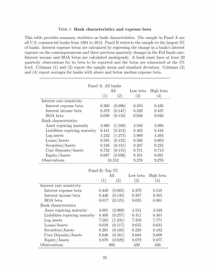
Table 1: Bank characteristics and expense beta

This table provides summary statistics on bank characteristics. The sample in Panel A areall U.S. commercial banks from 1984 to 2013. Panel B restricts the sample to the largest 5%of banks. Interest expense betas are calculated by regressing the change in a bank’s interestexpense on the contemporaneous and three previous quarterly changes in the Fed funds rate.Interest income and ROA betas are calculated analogously. A bank must have at least 20quarterly observations for its beta to be reported and the betas are winsorized at the 5%level. Columns (1) and (2) report the sample mean and standard deviation. Columns (3)and (4) report averages for banks with above and below median expense beta.

Panel A: All banksAll Low beta High beta

(1) (2) (3) (4)Interest rate sensitivity

Interest expense beta 0.360 (0.096) 0.283 0.436Interest income beta 0.379 (0.147) 0.320 0.437ROA beta 0.039 (0.150) 0.038 0.040

Bank characteristicsAsset repricing maturity 3.360 (1.580) 3.588 3.088Liabilities repricing maturity 0.441 (0.213) 0.462 0.416Log assets 4.232 (1.275) 3.969 4.494Loans/Assets 0.585 (0.132) 0.566 0.603Securities/Assets 0.246 (0.131) 0.267 0.225Core Deposits/Assets 0.732 (0.115) 0.751 0.713Equity/Assets 0.097 (0.036) 0.101 0.091

Observations 18,552 9,276 9,276

Panel B: Top 5%All Low beta High beta

(1) (2) (3) (4)Interest rate sensitivity

Interest expense beta 0.448 (0.085) 0.379 0.518Interest income beta 0.446 (0.135) 0.387 0.505ROA beta 0.017 (0.121) 0.035 0.001

Bank characteristicsAsset repricing maturity 4.001 (2.069) 4.551 3.349Liabilities repricing maturity 0.400 (0.257) 0.411 0.401Log assets 7.565 (1.231) 7.359 7.771Loans/Assets 0.628 (0.117) 0.625 0.631Securities/Assets 0.201 (0.103) 0.220 0.182Core Deposits/Assets 0.646 (0.161) 0.684 0.608Equity/Assets 0.078 (0.029) 0.079 0.077

Observations 860 430 430

33

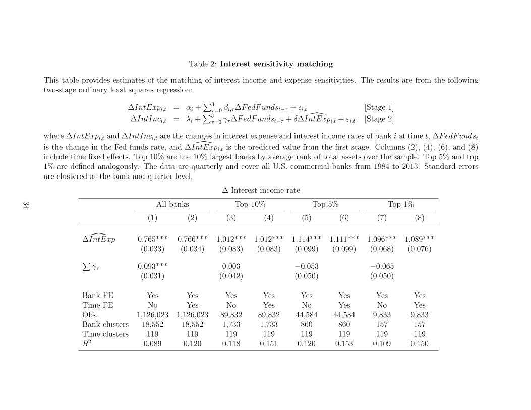
Table 2: Interest sensitivity matching

This table provides estimates of the matching of interest income and expense sensitivities. The results are from the followingtwo-stage ordinary least squares regression:

∆IntExpi,t = αi +∑3

τ=0 βi,τ∆FedFundst−τ + εi,t [Stage 1]

∆IntInci,t = λi +∑3

τ=0 γτ∆FedFundst−τ + δ ∆IntExpi,t + εi,t, [Stage 2]

where ∆IntExpi,t and ∆IntInci,t are the changes in interest expense and interest income rates of bank i at time t, ∆FedFundst

is the change in the Fed funds rate, and ∆IntExpi,t is the predicted value from the first stage. Columns (2), (4), (6), and (8)include time fixed effects. Top 10% are the 10% largest banks by average rank of total assets over the sample. Top 5% and top1% are defined analogously. The data are quarterly and cover all U.S. commercial banks from 1984 to 2013. Standard errorsare clustered at the bank and quarter level.

∆ Interest income rate

All banks Top 10% Top 5% Top 1%

(1) (2) (3) (4) (5) (6) (7) (8)

∆IntExp 0.765*** 0.766*** 1.012*** 1.012*** 1.114*** 1.111*** 1.096*** 1.089***(0.033) (0.034) (0.083) (0.083) (0.099) (0.099) (0.068) (0.076)∑

γτ 0.093*** 0.003 −0.053 −0.065(0.031) (0.042) (0.050) (0.050)

Bank FE Yes Yes Yes Yes Yes Yes Yes YesTime FE No Yes No Yes No Yes No YesObs. 1,126,023 1,126,023 89,832 89,832 44,584 44,584 9,833 9,833Bank clusters 18,552 18,552 1,733 1,733 860 860 157 157Time clusters 119 119 119 119 119 119 119 119R2 0.089 0.120 0.118 0.151 0.120 0.153 0.109 0.150

34

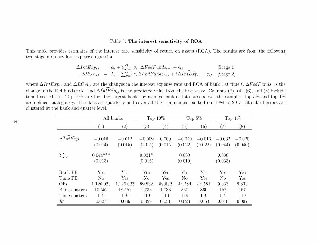
Table 3: The interest sensitivity of ROA

This table provides estimates of the interest rate sensitivity of return on assets (ROA). The results are from the followingtwo-stage ordinary least squares regression:

∆IntExpi,t = αi +∑3

τ=0 βi,τ∆FedFundst−τ + εi,t [Stage 1]

∆ROAi,t = λi +∑3

τ=0 γτ∆FedFundst−τ + δ ∆IntExpi,t + εi,t, [Stage 2]

where ∆IntExpi,t and ∆ROAi,t are the changes in the interest expense rate and ROA of bank i at time t, ∆FedFundst is the

change in the Fed funds rate, and ∆IntExpi,t is the predicted value from the first stage. Columns (2), (4), (6), and (8) includetime fixed effects. Top 10% are the 10% largest banks by average rank of total assets over the sample. Top 5% and top 1%are defined analogously. The data are quarterly and cover all U.S. commercial banks from 1984 to 2013. Standard errors areclustered at the bank and quarter level.

All banks Top 10% Top 5% Top 1%

(1) (2) (3) (4) (5) (6) (7) (8)

∆IntExp −0.018 −0.012 −0.009 0.000 −0.020 −0.013 −0.032 −0.020(0.014) (0.015) (0.015) (0.015) (0.022) (0.022) (0.044) (0.046)∑

γτ 0.044*** 0.031* 0.030 0.036(0.013) (0.016) (0.019) (0.033)

Bank FE Yes Yes Yes Yes Yes Yes Yes YesTime FE No Yes No Yes No Yes No YesObs. 1,126,023 1,126,023 89,832 89,832 44,584 44,584 9,833 9,833Bank clusters 18,552 18,552 1,733 1,733 860 860 157 157Time clusters 119 119 119 119 119 119 119 119R2 0.027 0.036 0.029 0.051 0.023 0.053 0.016 0.097

35

Table 4: Maturity transformation and expense betas

This table estimates the relationship between expense beta and asset duration. The proxyfor duration is repricing maturity, calculated as the weighted average repricing maturity ofloans and securities. The interest expense betas are estimated according to (7) and winsorizedat the 5% level. The control variables are wholesale funding (sum of large time deposits,Fed funds purchased, repos, and brokered deposits, divided by assets), equity ratio (equitydivided by assets), and log total assets. Top 5% of banks (Panel B) are the largest 5% byassets. The data are quarterly and cover all U.S. commercial banks with at least 5 years ofdata between 1997 to 2013. Standard errors are clustered at the bank and quarter level.

Panel A: All banks

Repricing maturity

(1) (2) (3) (4) (5)Interest expense beta −3.951*** −3.715*** −4.256*** −4.934*** −4.738***

(0.241) (0.238) (0.243) (0.246) (0.247)Wholesale funding ratio −0.616*** −1.052***

(0.180) (0.175)Equity ratio −3.482*** −2.467***

(0.485) (0.499)log Assets 0.238*** 0.236***

(0.017) (0.017)Time FE Yes Yes Yes Yes YesObservations 474,391 474,391 474,391 474,391 474,391Bank clusters 8,785 8,785 8,785 8,785 8,785Time clusters 67 67 67 67 67R2 0.118 0.119 0.122 0.139 0.143

Panel B: Top 5%

Repricing maturity

(1) (2) (3) (4) (5)Interest expense beta −4.676*** −5.346*** −5.405*** −5.027*** −6.136***

(1.323) (1.477) (1.285) (1.397) (1.489)Wholesale funding ratio 2.260 1.886

(1.400) (1.321)Equity ratio −13.470*** −12.814***

(1.983) (1.858)log Assets 0.055 0.072

(0.078) (0.078)Time FE Yes Yes Yes Yes YesObservations 13,445 13,445 13,445 13,445 13,445Bank clusters 267 267 267 267 267Time clusters 67 67 67 67 67R2 0.048 0.063 0.107 0.049 0.117

36

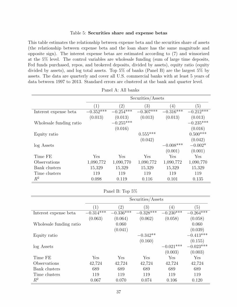
Table 5: Securities share and expense betas

This table estimates the relationship between expense beta and the securities share of assets(the relationship between expense beta and the loan share has the same magnitude andopposite sign). The interest expense betas are estimated according to (7) and winsorizedat the 5% level. The control variables are wholesale funding (sum of large time deposits,Fed funds purchased, repos, and brokered deposits, divided by assets), equity ratio (equitydivided by assets), and log total assets. Top 5% of banks (Panel B) are the largest 5% byassets. The data are quarterly and cover all U.S. commercial banks with at least 5 years ofdata between 1997 to 2013. Standard errors are clustered at the bank and quarter level.

Panel A: All banks

Securities/Assets

(1) (2) (3) (4) (5)Interest expense beta −0.352*** −0.254*** −0.307*** −0.316*** −0.212***

(0.013) (0.013) (0.013) (0.013) (0.013)Wholesale funding ratio −0.255*** −0.235***

(0.016) (0.016)Equity ratio 0.555*** 0.500***

(0.042) (0.042)log Assets −0.008*** −0.002*

(0.001) (0.001)Time FE Yes Yes Yes Yes YesObservations 1,090,772 1,090,770 1,090,772 1,090,772 1,090,770Bank clusters 15,329 15,329 15,329 15,329 15,329Time clusters 119 119 119 119 119R2 0.098 0.119 0.116 0.101 0.135

Panel B: Top 5%

Securities/Assets

(1) (2) (3) (4) (5)Interest expense beta −0.314*** −0.336*** −0.328*** −0.230*** −0.264***

(0.063) (0.064) (0.062) (0.058) (0.058)Wholesale funding ratio 0.060 0.060

(0.041) (0.039)Equity ratio −0.342** −0.413***

(0.160) (0.155)log Assets −0.021*** −0.023***

(0.003) (0.003)Time FE Yes Yes Yes Yes YesObservations 42,724 42,724 42,724 42,724 42,724Bank clusters 689 689 689 689 689Time clusters 119 119 119 119 119R2 0.067 0.070 0.074 0.106 0.120

37

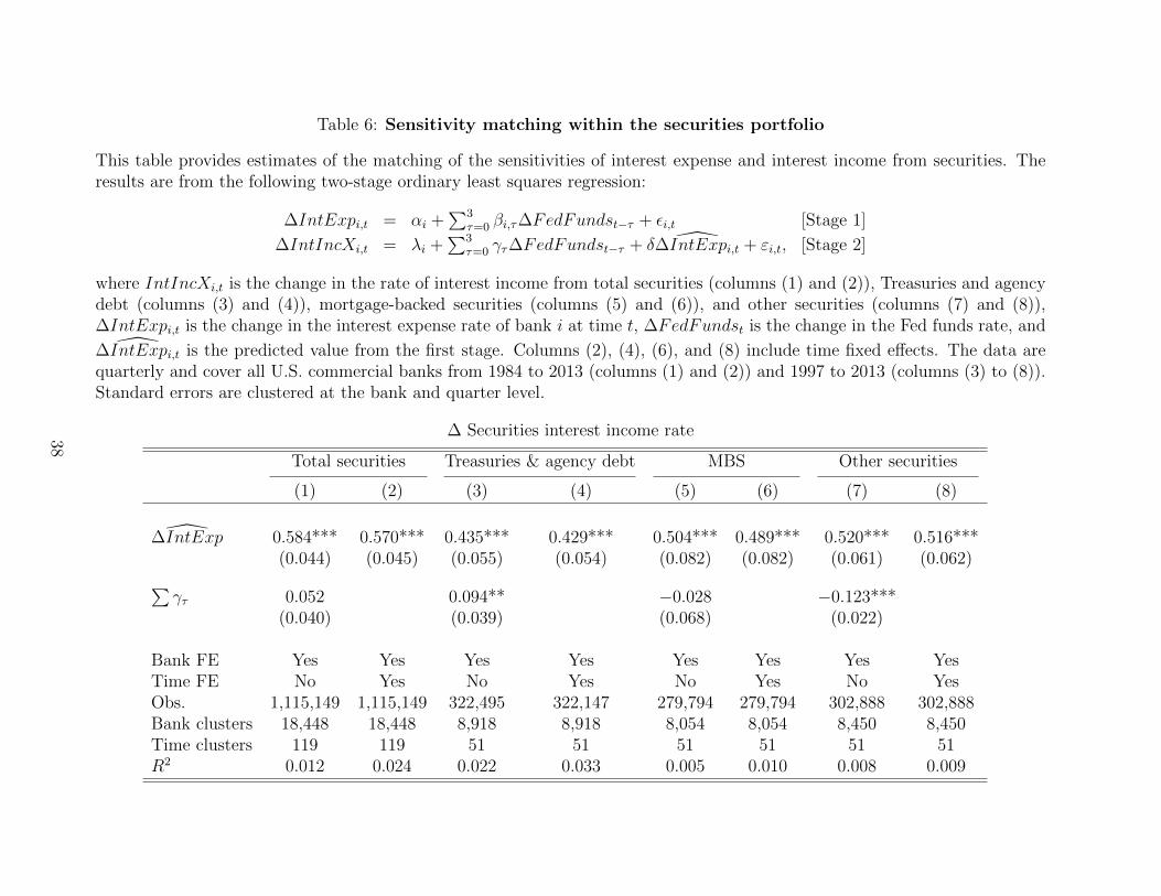
Table 6: Sensitivity matching within the securities portfolio

This table provides estimates of the matching of the sensitivities of interest expense and interest income from securities. Theresults are from the following two-stage ordinary least squares regression:

∆IntExpi,t = αi +∑3

τ=0 βi,τ∆FedFundst−τ + εi,t [Stage 1]

∆IntIncXi,t = λi +∑3

τ=0 γτ∆FedFundst−τ + δ ∆IntExpi,t + εi,t, [Stage 2]

where IntIncXi,t is the change in the rate of interest income from total securities (columns (1) and (2)), Treasuries and agencydebt (columns (3) and (4)), mortgage-backed securities (columns (5) and (6)), and other securities (columns (7) and (8)),∆IntExpi,t is the change in the interest expense rate of bank i at time t, ∆FedFundst is the change in the Fed funds rate, and

∆IntExpi,t is the predicted value from the first stage. Columns (2), (4), (6), and (8) include time fixed effects. The data arequarterly and cover all U.S. commercial banks from 1984 to 2013 (columns (1) and (2)) and 1997 to 2013 (columns (3) to (8)).Standard errors are clustered at the bank and quarter level.

∆ Securities interest income rate

Total securities Treasuries & agency debt MBS Other securities

(1) (2) (3) (4) (5) (6) (7) (8)

∆IntExp 0.584*** 0.570*** 0.435*** 0.429*** 0.504*** 0.489*** 0.520*** 0.516***(0.044) (0.045) (0.055) (0.054) (0.082) (0.082) (0.061) (0.062)∑

γτ 0.052 0.094** −0.028 −0.123***(0.040) (0.039) (0.068) (0.022)

Bank FE Yes Yes Yes Yes Yes Yes Yes YesTime FE No Yes No Yes No Yes No YesObs. 1,115,149 1,115,149 322,495 322,147 279,794 279,794 302,888 302,888Bank clusters 18,448 18,448 8,918 8,918 8,054 8,054 8,450 8,450Time clusters 119 119 51 51 51 51 51 51R2 0.012 0.024 0.022 0.033 0.005 0.010 0.008 0.009

38

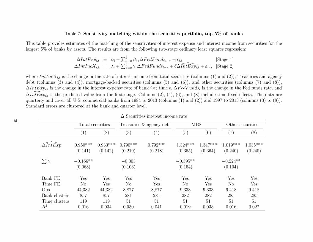
Table 7: Sensitivity matching within the securities portfolio, top 5% of banks

This table provides estimates of the matching of the sensitivities of interest expense and interest income from securities for thelargest 5% of banks by assets. The results are from the following two-stage ordinary least squares regression:

∆IntExpi,t = αi +∑3

τ=0 βi,τ∆FedFundst−τ + εi,t [Stage 1]

∆IntIncXi,t = λi +∑3

τ=0 γτ∆FedFundst−τ + δ ∆IntExpi,t + εi,t, [Stage 2]

where IntIncXi,t is the change in the rate of interest income from total securities (columns (1) and (2)), Treasuries and agencydebt (columns (3) and (4)), mortgage-backed securities (columns (5) and (6)), and other securities (columns (7) and (8)),∆IntExpi,t is the change in the interest expense rate of bank i at time t, ∆FedFundst is the change in the Fed funds rate, and

∆IntExpi,t is the predicted value from the first stage. Columns (2), (4), (6), and (8) include time fixed effects. The data arequarterly and cover all U.S. commercial banks from 1984 to 2013 (columns (1) and (2)) and 1997 to 2013 (columns (3) to (8)).Standard errors are clustered at the bank and quarter level.

∆ Securities interest income rate

Total securities Treasuries & agency debt MBS Other securities

(1) (2) (3) (4) (5) (6) (7) (8)

∆IntExp 0.950*** 0.933*** 0.790*** 0.792*** 1.324*** 1.347*** 1.019*** 1.035***(0.141) (0.142) (0.219) (0.218) (0.355) (0.364) (0.240) (0.240)∑

γτ −0.166** −0.003 −0.395** −0.224**(0.068) (0.103) (0.154) (0.104)

Bank FE Yes Yes Yes Yes Yes Yes Yes YesTime FE No Yes No Yes No Yes No YesObs. 44,382 44,382 8,877 8,877 9,333 9,333 9,418 9,418Bank clusters 857 857 281 281 282 282 285 285Time clusters 119 119 51 51 51 51 51 51R2 0.016 0.034 0.030 0.041 0.019 0.038 0.016 0.022

39

Table 8: Market power and interest sensitivity matching

This table estimates the effect of market power on interest rate sensitivity matching. Theresults are from the following two-stage ordinary least squares regression:

∆IntExpi,t = αi + φXi,t +∑3

τ=0 (β0τ + βτXi,t) ∆FedFundst−τ + εi,t [Stage 1]

∆IntInci,t = λi +∑3

τ=0 γτ∆FedFundst−τ + δ ∆IntExpi,t + εi,t, [Stage 2]

where Xi,t is bank i’s market concentration, ∆IntExpi,t and ∆IntInci,t are the changes ininterest expense and interest income rates of bank i at time t, ∆FedFundst is the change in

the Fed funds rate, and ∆IntExpi,t is the predicted value from the first stage. To calculatemarket concentration, we construct a Herfindahl index of bank branches at the zip codelevel (columns (1) and (2)) or county level (columns (3) and (4)), then average them acrosseach bank’s branches, using branch deposit as weights. Columns (2), and (4) include timefixed effects. The data are quarterly and cover all U.S. commercial banks from 1994 to 2013.Standard errors are clustered at the bank and quarter level.

Market concentration Market concentration(zip code) (county)

(1) (2) (3) (4)

Stage 1: ∆ Interest expense rate

∑βτ −0.047*** −0.059*** −0.047** −0.065***

(0.021) (0.016) (0.023) (0.016)

R2 0.196 0.237 0.194 0.234

Stage 2: ∆ Interest income rate

∆IntExp 1.264*** 1.278*** 0.921*** 0.838***(0.186) (0.154) (0.308) (0.250)∑

γτ −0.044 −0.060(0.071) (0.069)

Bank FE Yes Yes Yes YesTime FE No Yes No YesR2 0.088 0.122 0.087 0.12Observations 624,204 624,204 624,204 624,204Bank clusters 13,010 13,010 13,010 13,010Time clusters 80 80 80 80

40

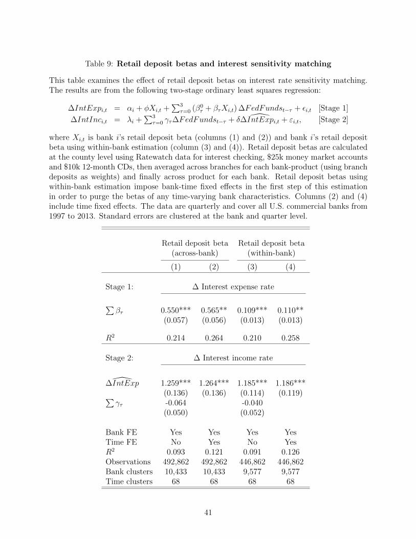
Table 9: Retail deposit betas and interest sensitivity matching

This table examines the effect of retail deposit betas on interest rate sensitivity matching.The results are from the following two-stage ordinary least squares regression:

∆IntExpi,t = αi + φXi,t +∑3

τ=0 (β0τ + βτXi,t) ∆FedFundst−τ + εi,t [Stage 1]

∆IntInci,t = λi +∑3

τ=0 γτ∆FedFundst−τ + δ ∆IntExpi,t + εi,t, [Stage 2]

where Xi,t is bank i’s retail deposit beta (columns (1) and (2)) and bank i’s retail depositbeta using within-bank estimation (column (3) and (4)). Retail deposit betas are calculatedat the county level using Ratewatch data for interest checking, $25k money market accountsand $10k 12-month CDs, then averaged across branches for each bank-product (using branchdeposits as weights) and finally across product for each bank. Retail deposit betas usingwithin-bank estimation impose bank-time fixed effects in the first step of this estimationin order to purge the betas of any time-varying bank characteristics. Columns (2) and (4)include time fixed effects. The data are quarterly and cover all U.S. commercial banks from1997 to 2013. Standard errors are clustered at the bank and quarter level.

Retail deposit beta Retail deposit beta(across-bank) (within-bank)

(1) (2) (3) (4)

Stage 1: ∆ Interest expense rate

∑βτ 0.550*** 0.565** 0.109*** 0.110**

(0.057) (0.056) (0.013) (0.013)

R2 0.214 0.264 0.210 0.258

Stage 2: ∆ Interest income rate

∆IntExp 1.259*** 1.264*** 1.185*** 1.186***(0.136) (0.136) (0.114) (0.119)∑

γτ -0.064 -0.040(0.050) (0.052)

Bank FE Yes Yes Yes YesTime FE No Yes No YesR2 0.093 0.121 0.091 0.126Observations 492,862 492,862 446,862 446,862Bank clusters 10,433 10,433 9,577 9,577Time clusters 68 68 68 68

41

Figure 1: Industry-level stock returns and interest rate changes

The figure shows the sensitivity of bank and other industry stock portfolios to FOMC rate changes. The data are the returns ofthe Fama-French 49 industry portfolios and the CRSP value-weighted market portfolio, downloaded from Ken French’s website.The figure plots the coefficients from regressions of these industry returns on the change in the one-year Treasury rate (obtainedfrom the Fed’s H.15 release) over a two-day window around FOMC meetings as in Hanson and Stein (2015). The sampleincludes all scheduled FOMC meetings from 1994 to 2008 (there are 113 such meetings and 5 unscheduled ones).

42

Figure 2: Aggregate time series

The figure plots the aggregate time series of net interest margin (NIM) and return on assets(ROA) in Panel A, and the interest income and interest expense rates in Panel B. Also shownis the Fed funds rate. The interest income and expense rates equal total interest income andexpense divided by assets, respectively. The data are annual from FDIC, 1955 to 2015.

Panel A: NIM and ROA

0%

6%

12%

18%

1955 1960 1965 1970 1975 1980 1985 1990 1995 2000 2005 2010

Fed funds rate Net interest margin ROA

Panel B: Interest income and interest expense rate

0%

6%

12%

18%

1955 1960 1965 1970 1975 1980 1985 1990 1995 2000 2005 2010

Fed funds rate Interest income rate Interest expense rate

43

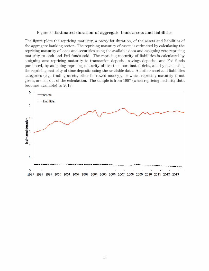
Figure 3: Estimated duration of aggregate bank assets and liabilities

The figure plots the repricing maturity, a proxy for duration, of the assets and liabilities ofthe aggregate banking sector. The repricing maturity of assets is estimated by calculating therepricing maturity of loans and securities using the available data and assigning zero repricingmaturity to cash and Fed funds sold. The repricing maturity of liabilities is calculated byassigning zero repricing maturity to transaction deposits, savings deposits, and Fed fundspurchased, by assigning repricing maturity of five to subordinated debt, and by calculatingthe repricing maturity of time deposits using the available data. All other asset and liabilitiescategories (e.g. trading assets, other borrowed money), for which repricing maturity is notgiven, are left out of the calculation. The sample is from 1997 (when repricing maturity databecomes available) to 2013.

44

Figure 4: The distributions of interest expense and income betas

The interest expense and income betas are calculated by regressing the change in abank’s interest expense or income rate on the contemporaneous and previous three quar-terly changes in the Fed funds rate. The sample includes all banks with at least20 quarterly obervations. For this figure, the betas are winsorized at the 1% level.

01

23

4D

ensi

ty

-.2 0 .2 .4 .6 .8 1Interest expense beta

01

23

4D

ensi

ty

-.2 0 .2 .4 .6 .8 1Interest income beta

45

Figure 5: Interest expense, interest income, and ROA matching

This figure shows bin scatter plots of interest expense, interest income, and ROA betas forall banks and the largest five percent of banks. The betas are calculated by regressing thequarterly change in each bank’s interest expense rate, interest income rate, or ROA on thecontemporaneous and previous three changes in the Fed funds rate. Only banks with atleast 20 quarterly observations are included. The betas are winsorized at the 5% level. Thebin scatter plot groups banks into 100 bins by interest expense beta and plots the averageincome or ROA beta within each bin. The top 5% percent of banks are those whose averagepercentile rank by assets over the sample is below the fifth percentile. The sample is from1984 to 2013.

All banks Top 5%

.1.2

.3.4

.5.6

Inte

rest

inco

me

beta

.1 .2 .3 .4 .5 .6Interest expense beta

Coef. = 0.768, R-sq. = 0.264

.2.3

.4.5

.6.7

Inte

rest

inco

me

beta

.2 .3 .4 .5 .6 .7Interest expense beta

Coef. = 0.878, R-sq. = 0.338

-.2-.1

0.1

.2R

OA

bet

a

.1 .2 .3 .4 .5 .6Interest expense beta

Coef. = 0.061, R-sq. = 0.001

-.2-.1

0.1

.2R

OA

bet

a

.2 .3 .4 .5 .6 .7Interest expense beta

Coef. = -0.191, R-sq. = 0.023

46

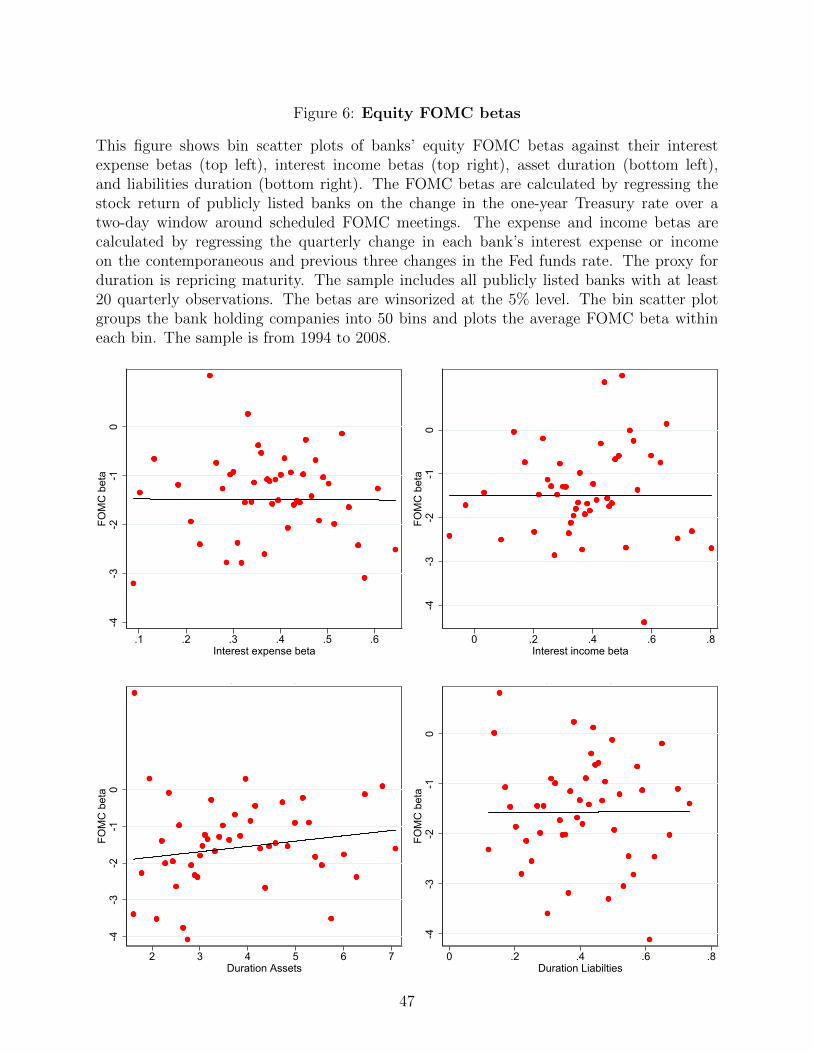
Figure 6: Equity FOMC betas

This figure shows bin scatter plots of banks’ equity FOMC betas against their interestexpense betas (top left), interest income betas (top right), asset duration (bottom left),and liabilities duration (bottom right). The FOMC betas are calculated by regressing thestock return of publicly listed banks on the change in the one-year Treasury rate over atwo-day window around scheduled FOMC meetings. The expense and income betas arecalculated by regressing the quarterly change in each bank’s interest expense or incomeon the contemporaneous and previous three changes in the Fed funds rate. The proxy forduration is repricing maturity. The sample includes all publicly listed banks with at least20 quarterly observations. The betas are winsorized at the 5% level. The bin scatter plotgroups the bank holding companies into 50 bins and plots the average FOMC beta withineach bin. The sample is from 1994 to 2008.

-4-3

-2-1

0FO

MC

bet

a

.1 .2 .3 .4 .5 .6Interest expense beta

Coef. = -0.042 (s.e. = 1.080), R-sq. = 0.000

-4-3

-2-1

0FO

MC

bet

a

0 .2 .4 .6 .8Interest income beta

Coef. = 0.004 (s.e. = 0.711), R-sq. = 0.000

-4-3

-2-1

0FO

MC

bet

a

2 3 4 5 6 7Duration Assets

Coef. = 0.145 (s.e. = 0.102), R-sq. = 0.003

-4-3

-2-1

0FO

MC

bet

a

0 .2 .4 .6 .8Duration Liabilties

Coef. = 0.041 (s.e. = 0.943), R-sq. = 0.000

47

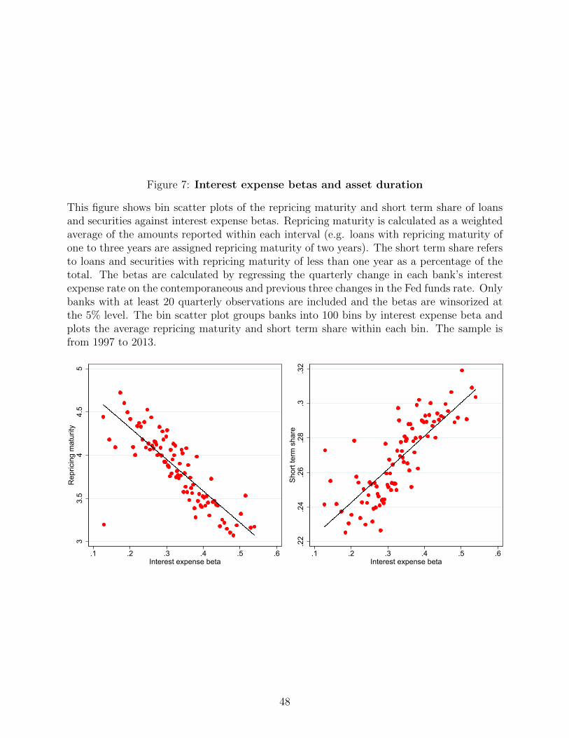
Figure 7: Interest expense betas and asset duration

This figure shows bin scatter plots of the repricing maturity and short term share of loansand securities against interest expense betas. Repricing maturity is calculated as a weightedaverage of the amounts reported within each interval (e.g. loans with repricing maturity ofone to three years are assigned repricing maturity of two years). The short term share refersto loans and securities with repricing maturity of less than one year as a percentage of thetotal. The betas are calculated by regressing the quarterly change in each bank’s interestexpense rate on the contemporaneous and previous three changes in the Fed funds rate. Onlybanks with at least 20 quarterly observations are included and the betas are winsorized atthe 5% level. The bin scatter plot groups banks into 100 bins by interest expense beta andplots the average repricing maturity and short term share within each bin. The sample isfrom 1997 to 2013.

33.

54

4.5

5R

epric

ing

mat

urity

.1 .2 .3 .4 .5 .6Interest expense beta

Coef. = -3.662, R-sq. = 0.052

.22

.24

.26

.28

.3.3

2S

hort

term

sha

re

.1 .2 .3 .4 .5 .6Interest expense beta

Coef. = 0.193, R-sq. = 0.027

48

Figure 8: Interest expense betas and market concentration

This figure presents a bin scatter plot of interest expense betas against a bank Herfindahl(HHI) index. To calculate the bank HHI, we first calculate a zip-code HHI by computingeach bank’s share of the total branches in the zip code and summing the squared shares. Wethen create the bank HHI by averaging the zip-code HHIs of each bank’s branches, usingthe bank’s deposits in each zip code as weights. The betas are calculated by regressingthe change in a bank’s interest expense rate on the contemporaneous and previous threequarterly changes in the Fed funds rate. Only banks with at least 20 quarterly observationsare included. The betas are winsorized at the 5% level. The sample covers 1994 to 2013.

.28

.3.3

2.3

4.3

6.3

8In

tere

st e

xpen

se b

eta

0 .2 .4 .6 .8 1Bank HHI

Coef. = -0.079, R-sq. = 0.039

49

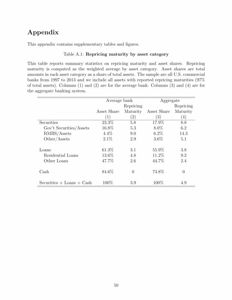
Appendix

This appendix contains supplementary tables and figures.

Table A.1: Repricing maturity by asset category

This table reports summary statistics on repricing maturity and asset shares. Repricingmaturity is computed as the weighted average by asset category. Asset shares are totalamounts in each asset category as a share of total assets. The sample are all U.S. commercialbanks from 1997 to 2013 and we include all assets with reported repricing maturities (97%of total assets). Columns (1) and (2) are for the average bank. Columns (3) and (4) are forthe aggregate banking system.

Average bank AggregateRepricing Repricing

Asset Share Maturity Asset Share Maturity(1) (2) (3) (4)

Securities 23.3% 5.8 17.9% 8.8Gov’t Securities/Assets 16.8% 5.3 8.0% 6.2RMBS/Assets 4.4% 9.0 6.2% 14.3Other/Assets 2.1% 2.9 3.6% 5.1

Loans 61.3% 3.1 55.9% 3.8Residential Loans 13.6% 4.8 11.2% 9.2Other Loans 47.7% 2.6 44.7% 2.4

Cash 84.6% 0 73.8% 0

Securities + Loans + Cash 100% 3.9 100% 4.9

50

Table A.2: Interest sensitivity matching and derivatives usage

This table estimates the same regressions as in Table 2 for the sub-samples that do anddo not use interest rate derivatives. Columns 1 and 2 provide results for all banks withnon-missing derivatives data (this data starts in 1995). Columns 3 and 4 present results forbanks that have zero exposure to derivatives. Columns 5 and 6 present results for banksthat have nonzero exposure to derivatives.

∆ Interest income rate

All banks No derivatives Nonzero derivatives

(1) (2) (3) (4) (5) (6)

∆IntExp 1.108*** 1.114*** 1.096*** 1.104*** 1.305*** 1.323***(0.056) (0.055) (0.055) (0.054) (0.071) (0.073)∑

γτ −0.011 −0.007 −0.090**(0.030) (0.029) (0.039)

Bank FE Yes Yes Yes Yes Yes YesTime FE No Yes No Yes No YesObs. 563,955 563,955 521,021 521,021 37,163 37,163Bank clusters 12,073 12,073 11,754 11,754 2,192 2,192Time clusters 75 75 75 75 75 75R2 0.137 0.172 0.144 0.180 0.219 0.246

51

Table A.3: Interest sensitivity matching for bank holding companies (BHC)

This table examines whether bank holding companies match the interest rate sensitivity of their income and expenses. Theresults are from the following two-stage ordinary least squares regression of interest income rates on interest expense rates:

∆IntExpi,t = αi +∑3

τ=0 βi,τ∆FedFundst−τ + εi,t [Stage 1]

∆IntInci,t = λi +∑3

τ=0 γτ∆FedFundst−τ + δ ∆IntExpi,t + εi,t. [Stage 2]

Columns (2), (4), (6), and (8) include time fixed effects. Top 10% of banks are those that have a top-10% average rank byassets over the sample. Top 5% and top 1% of banks are defined analogously. The data are quarterly and cover all U.S. BHCsfrom 1989 to 2013. Standard errors are clustered at the bank and quarter level..

∆ Interest income rate

All BHC Top 10% Top 5% Top 1%

(1) (2) (3) (4) (5) (6) (7) (8)

∆IntExp 1.063*** 1.055*** 1.117*** 1.106*** 1.117*** 1.105*** 1.071*** 0.995***(0.071) (0.070) (0.118) (0.120) (0.177) (0.182) (0.145) (0.153)∑

γτ −0.026 −0.098* −0.108 −0.089(0.031) (0.056) (0.090) (0.090)

Bank FE Yes Yes Yes Yes Yes Yes Yes YesTime FE No Yes No Yes No Yes No YesObs. 143,013 143,013 13,223 13,223 6,761 6,761 1,218 1,218Bank clusters 4,232 4,232 322 322 162 162 28 28Time clusters 108 108 108 108 108 108 108 108R2 0.175 0.217 0.159 0.213 0.151 0.219 0.165 0.368

52

Figure A.1: Estimated duration of bank assets and liabilities

The figure plots the distribution of repricing maturity, a proxy for duration, of bank assetsand liabilities. The repricing maturity of assets is estimated by calculating the repricingmaturity of loans and securities using the available data and assigning zero repricing maturityto cash and Fed funds sold. The repricing maturity of liabilities is calculated by assigningzero repricing maturity to transaction deposits, savings deposits, and Fed funds purchased,by assigning repricing maturity of five to subordinated debt, and by calculating the repricingmaturity of time deposits using the available data. All other asset and liabilities categories(e.g. trading assets, other borrowed money), for which repricing maturity is not given, areleft out of the calculation. The sample is from 1997 to 2013.

All banks

0.5

11.

52

Den

sity

0 1 2 3 4 5 6 7 8Repricing maturity

Liabilities Assets

Top 5%

0.5

11.

52

2.5

Den

sity

0 1 2 3 4 5 6 7 8Repricing maturity

Liabilities Assets

53

Figure A.2: The interest rate sensitivity of operating costs and fee income

This figure shows bin scatter plots of bank operating costs and deposit fee income by expensebetas. The betas and scatterplots are constructed the same was as in Figure 5. The leftcolumn is for all banks and the right column for the top five percent of banks. The top panelprovides information on total salaries, the middle panel on total rent, and the bottom panelon deposit fee income.

All banks Top 5%

Panel A: Total salaries

-.2-0

.10

.1.2

Cos

t Bet

a

.1 .2 .3 .4 .5 .6Interest Expense beta

Coef. = -0.095, R-sq. = 0.025

-.2-0

.10

.1.2

Cos

t Bet

a

.2 .3 .4 .5 .6 .7Interest Expense beta

Coef. = 0.032, R-sq. = 0.004

Panel B: Total rent

-.2-0

.10

.1.2

Cos

t Bet

a

.1 .2 .3 .4 .5 .6Interest Expense beta

Coef. = -0.030, R-sq. = 0.007

-.2-0

.10

.1.2

Cos

t Bet

a

.2 .3 .4 .5 .6 .7Interest Expense beta

Coef. = 0.009, R-sq. = 0.001

Panel C: Deposit fee income

-.2-0

.10

.1.2

Fee

Inco

me

Bet

a

.1 .2 .3 .4 .5 .6Interest expense beta

Coef. = 0.002, R-sq. = 0.000

-.2-0

.10

.1.2

Fee

Inco

me

Bet

a

.2 .3 .4 .5 .6 .7Interest expense beta

Coef. = 0.011, R-sq. = 0.007

54