FEDERAL RESERVE BANK OF SAN FRANCISCO

WORKING PAPER SERIES

Bank Relationships, Business Cycles, and Financial Crises

Galina Hale

Federal Reserve Bank of San Francisco

July 2011

Working Paper 2011-14 http://www.frbsf.org/publications/economics/papers/2011/wp11-14bk.pdf

The views in this paper are solely the responsibility of the authors and should not be interpreted as reflecting the views of the Federal Reserve Bank of San Francisco or the Board of Governors of the Federal Reserve System.

Bank Relationships, Business Cycles, and Financial Crises

Galina Hale∗

Federal Reserve Bank of San Francisco

July 29, 2011

Abstract

The importance of information asymmetries in the capital markets is commonly accepted asone of the main reasons for home bias in investment. We posit that effects of such asymmetriesmay be reduced through relationships between banks established through bank-to-bank lendingand provide evidence to support this claim. We construct a global banking network of 7938banking institutions from 141 countries to analyze the formation of new relationships betweenbanks during 1980-2009 time period. We find that recessions and banking crises tend to havenegative effects on the formation of new connections and that these effects are not the same forall countries or all banks. We also find that the global financial crisis of 2008-09 had a largenegative impact on the formation of new relationships in the global banking network.

JEL classification: F34, F36

Key words: networks, international banking, crises, bank relationships

∗Galina.b.hale@sf.frb.org.I am grateful to Hiro Miura and Chris Candelaria for outstanding research assistance, to Joshua Aizenman for veryhelpful conversations, to Matthieu Bussiere, Kristin Forbes, Reuven Glick, Charles Engel, Oscar Jorda, Jean Imbs, aswell as the participants at a preconference at the NBER Summer Institute 2010, seminars at the Federal Reserve Bankof San Francisco and the Banque de France, and IBEFA session at 2011 AEA meetings for constructive comments andsuggestions. I am grateful to Anita Todd for help with preparing the draft. All errors are mine. All views presentedin this paper are mine and do not necessarily represent the views of the Federal Reserve Bank of San Francisco orFederal Reserve Board of Governors.

1

1 Introduction

International finance literature has long emphasized the importance of information in international

investment, citing information asymmetry as one of the leading explanations for portfolio home

bias and lack of international diversification.1 Financial globalization created a number of avenues

through which the effects of asymmetric information can potentially be reduced. One of them is

international banking in general and lending of banks to each other in particular.2 It is commonly

accepted that bank lending to corporate borrowers establishes the relationship and produces infor-

mation flows between the lender and the borrower, which in turn facilitate further lending.3 It is

thus reasonable to believe that lending of one bank to another establishes a channel for information

flows between the lender and the borrower that might facilitate future lending, international capital

flows of other types, as well as international trade.

Recent global financial crisis had a major impact on the global banking system (Milesi-Ferretti

& Tille, 2011). But did the crisis simply affect the volume of bank lending or did it also affect the

structure of international banking system? If relationships between banks play a role, implications

of these two developments are not identical. The aim of this paper, therefore, is to investigate the

impact of the global financial crisis, as well as of country-specific recessions and banking crises of

the past 30 years on the formation of new relationships between banks and the importance of banks

in the affected country. To achieve our goal, we use micro-level data on international syndicated

bank loans from Loan Analytics database to construct a bank-level global banking network (GBN)

1A number of models of international portfolio flows rely on the assumption of information asymmetry betweenlocal and foreign markets (Brennan & Cao, 1997; Okawa & Van Wincoop, 2010). Portes et al. (2001) and Portes &Rey (2005) provide direct evidence of the importance of information in determining bilateral patterns of aggregateinternational capital flows, while Kang & Stulz (1997) and Hatchondo (2008) show that such patterns are consistentwith the model that is based on asymmetric information. Local informational advantages have also been documentedin various contexts in finance literature (Ahearne et al., 2004; Bae et al., 2008; Chan et al., 2008; Coval & Moscowitz,2001; Huberman, 2001). Veldcamp & Van Nieuwerburgh (2009) present a theoretical argument for persistence ofinformation asymmetry.

2Milesi-Ferretti & Tille (2011) emphasize prominent growth of international banking prior to the global financialcrisis.

3See survey by Boot (2000).

2

and analyze the dynamics of its structure. This is the first study in which bank-level network is

analyzed in a global scale.4

We construct a global network of banks in which relationships are formed by banks extending

loans to each other, taking into account the direction of the lending. Because we are interested

in the dynamics of these network statistics, we construct two panel data sets, each at bank-year

level. One, noncumulative panel, consists of separate new networks based on loans made in each of

the years between 1980 and 2009 thus providing snapshots of lending patterns for each year. The

other, cumulative panel is constructed by adding new loans to the network that starts in 1980 and

expands through 2009, allowing us to distinguish old and new relationships. For each bank in each

year we compute the number of direct lending and borrowing connections, i.e. number of borrowers

and lenders, and identify whether the this bank in a given year played a role as a key intermediary,

that is whether it was the only bank connecting at least one pair of other banks to each other.

To verify that relationships between banks defined by lending of one bank to another have

indeed an effect on lending and borrowing, we demonstrate, in a bank-level fixed effects regression,

that establishing a new relationship increases the amount of new loan origination to or by this

bank in the following three years. Moreover, in a country-level fixed effects regression, we find that

when the number of key banks in a given country increases, that country experiences an increase in

both lending and borrowing in at least four years that follow. In a related study, Hale et al. (2011)

provide evidence that connections between banks, as defined in this paper, are positively related

to international FDI and portfolio flows. Finally, there is evidence that countries in which banks

were more connected to other banks through syndicated loan market experienced a lesser impact

of the global financial crisis (Caballero et al., 2009).

We next describe the dynamics of the overall network size and connectivity over our sample

4In the existing literature, either global network is analyzed at a country level (Garratt et al., 2011; Kubelec &Sa, 2010; Minoiu & Reyes, 2011; von Peter, 2007) or bank-level network is constructed for a specific country (Coccoet al., 2009; Craig & von Peter, 2010).

3

period. We find that since the 1980s the global banking network experienced two major periods

of rapid expansion — one in the early 1990s and one between 2002 and 2006. These periods of

expansion were characterized by an increasing number of banks, increasing number of connections

between banks, and increasing number of countries in which banks participate in the GBN. Im-

portantly, network expansion during these periods was achieved more through formation of new

connections by existing banks than trough an increase in the number of banks. We also observe

that formation of new connections and the share of banks that are key intermediaries tend to de-

cline during recessions in the United States. We very clearly observe a collapse of the GBN during

the global financial crisis that brought most measures of the network back to the level that was

observed prior to the 2002-2006 expansion.

Before turning to the regression analysis of bank-level network statistics, we present a stylized

two-country model of bank relationships that arise endogenously and respond to shocks such as

demand, supply, and cost of capital. The model predicts that local recessions in small countries

can increase the number of new connections established between the banks initially, but will lower

them in the long run. A recession in the United States (a larger country and “the world banker”)

would increase the number of new connections made because U.S. banks would seek investment

abroad. A local systemic banking crisis in a small country, represented by an increase in the cost

of funding in this country, would lead to an increase in the number of new relationships formed. A

global banking crisis, however, if thought of as a decline in the value of future relationships, would

result in fewer new connections.

To study the effects of country-specific recessions and banking crises and to control for the

effects of total lending and borrowing when studying the effects of the global financial crisis, we

turn to the regression analysis. Because we are interested in the effects on new connections, we

conduct our regression analysis using the cumulative network. We find that, conditional on total

borrowing and lending, local recessions lead to fewer new connections made by banks in the affected

4

country, especially banks that are smaller or that are located in developing countries. We find that

local banking crises have a negative effect on the formation of new borrowing connections.5 During

the recessions in the U.S. large banks are more likely to find new borrowers and establish more new

lending connections than during other times. In addition, the number of new key banks tends to

fall in countries that experience recessions.

We find a large negative effect of the global financial crisis on the formation of new connections,

which was felt most strongly through a decline in entry of new banks from developing countries into

the GBN and decline in the number of connections made, especially by large banks.6 We also find

that the formation of new key banks declined and moved from developing to industrial countries

during the crisis. These effects of the global financial crisis are conditional on total lending and

borrowing as well as on the effects of local recessions that occurred in most countries in our sample

during crisis years.

We make the following conclusions from the analysis. Recessions and as banking crises have an

important effect on the development of the global banking network through lowering the number of

new connections banks make and the distribution of these connections across banks and countries.

Thus, we show that in addition to real costs of banking crises (Reinhart & Rogoff, 2009; Schularick

& Taylor, 2010), there are costs associated with deterioration of bank relationships. Furthermore,

we show that the effects of the global financial crisis on the global banking network were especially

large and unevenly distributed across banks and countries. Importantly, fewer banks during the

crisis played key intermediation roles, especially in developing countries. Combined with the finding

that new relationships and the number of key banks tend to have a persistent effect on borrowing

and lending, our results provide an additional mechanism that may partly explain the collapse

in international capital flows during the crisis and the fact that it was especially pronounced in

5This finding is consistent with that in Peek & Rosengren (2000) for the case of Japan.6As Rose & Wieladek (2011) demonstrate, some of this decline may be due to an increase in financial protectionism

associated with massive injections of public funds into banks during the crisis.

5

emerging markets (Milesi-Ferretti & Tille, 2011).7

Our paper also has a methodological implication for the active literature on the stability of

banking network. Many recent papers on financial networks analyze the potential for the spread

of contagion in various exogenous network structures using simulation methods (Battiston et al.,

2009; May & Arinaminpathy, 2010; Mirchev et al., 2010; Nier et al., 2007; Sachs, 2010). Others em-

pirically analyze the structure or the development of country-specific and global banking networks

(Cocco et al., 2009; Craig & von Peter, 2010; Garratt et al., 2011; von Peter, 2007). A handful of

papers model how relationships between banks form networks endogenously (Allen & Gale, 2000;

Castiglionesi & Navarro, 2007; Delli Gatti et al., 2010). The findings of our paper contribute to

this literature by showing that the structure of a global banking network responds to economic and

financial shocks, and therefore it may not be appropriate to model banking networks as static or

exogenous, especially when analyzing the effects of financial shocks.

The paper is organized as follows. Section 2 presents our data and methodology, mostly

focusing on the construction of the global banking network and the network statistics. Section 3

describes the evolution of the network structure over time. Section 4 presents a stylized model

of the formation of bank relationships. Section 5 presents the results of our regression analysis.

Section 6 concludes.

2 Constructing global banking network

In the wake of the global financial crisis, the complex structure of bank relationships started to

garner attention in the literature. One direction of this analysis turned to representing banking sys-

tems as graphs, or networks.8 This literature mostly focuses on the short-run aspects of connections

7For comprehensive analysis of factors affecting global capital flows during the crisis and the recovery, see Fratzscher(2011).

8Some recent papers are Chan-Lau et al. (2009); Haldane (2009) and Haldane & May (2011). The applicationof the network approach to financial markets follows recent literature on networks in social interactions and firm

6

between banks, that is, liquidity exposures of banks to one another, the topology of which affects

the stability of the banking system and the propagation of the shocks. As discussed above, in this

paper we take a longer-run view of connections between banks, interpreting lending relationships

as connections that facilitate information flows.

Unlike much of the recent empirical analysis of banking and financial networks that build

on aggregate country-level bilateral bank lending from the Bank for International Settlements

(BIS) data and bilateral asset holdings from the International Monetary Fund’s (IMF) Coordinated

Portfolio Investment Survey (CPIS) (Garratt et al., 2011; Kubelec & Sa, 2010; Minoiu & Reyes,

2011; von Peter, 2007), this paper constructs a global banking network at the bank level, something

that has not been done before.9 There are two main reasons why loan-level data are more suitable

for the construction of the network than BIS statistics. First, the BIS reports stocks of claims and

does not provide information on the origination time of these claims. The BIS computes “flows”

as a change in stocks, and therefore such flows include, in addition to loan origination, repayments

and changes in valuations of these stocks. As a result, such data cannot provide clean information

on the formation of new relationships between banks (or countries, in case of BIS data). Second,

country-level data do not distinguish between cases with many loans of smaller amounts made in

many different pairs of banks and cases where only a few large loans are made between a small

number of bank pairs. Loan-level data address both of these concerns — they give the date of the

loan origination and allow us to compute network statistics at the bank level.

We assume that each loan from bank to bank creates a relationship, or link, thus contributing

to the network. Our data consist of syndicated bank loans with median maturity of about 5 years.

theory. Karlan et al. (2009) offers a theoretical model of networks in social interactions, while papers by Bottazziet al. (2009); Guiso et al. (2009) and Lehmann & Neuberger (2001) provide some discussion of the importance oftrust and social interactions for investment, economic exchange, and lending. The work on social capital pioneeredby Putnam (1995) is the seed of much of this literature.

9Craig & von Peter (2010) use data from the German interbank market to test for tiering in the banking network;Cocco et al. (2009) build, for the Portuguese interbank market, “borrower preference” and “lender preference” indexesbased on loans between banks, but do not go so far as to create a network of banks, which would take into accountindirect relationships.

7

Thus, the relationships we define are long-term relationships between banks. In constructing a

cumulative network panel by adding new loans to the ones that existed in the prior year we implicitly

make an assumption that relationships between banks that are established through lending persist

even if the loan is repayed.

2.1 Data sources and manipulation

Dealogic’s Loan Analytics database (a.k.a. Loanware) provides information on international syn-

dicated bank loans (with some domestic syndicated loans included as well). It has exhaustive

information on the terms of the loan, as well as some information on borrowers and lenders. From

this database, we downloaded information on loans extended between January 1, 1980, and De-

cember 31, 2009, to private- and public-sector banks, a total of 15,324 loans. Out of these, 84 loans

had to be dropped due to missing deal values and 151 had to be dropped due to missing lenders

field, which left us with the total of 15089 loans.

The Loan Analytics database provides information on syndicated bank loan origination, includ-

ing loans extended to financial institutions. For our purposes, syndicated loans are a good proxy

for bank relationships because they tend to be of much longer maturities than interbank loans and

thus represent a larger commitment and the potential for information flows. The bank-to-bank

syndicated loan market is relatively large — in the late 1990s syndicated bank loans extended to

banks and reported in Loan Analytics amounted to over 30 percent of total bank claims on banks

as reported by the BIS. This ratio fell to below 20 percent by the end of our sample as interbank

lending ballooned prior to the global financial crisis. In 2007, prior to the crisis, 4.7 trillion USD

worth of syndicated loans were extended to banks (see Figure 1).10

10BIS reports in its Table 10 in the Annex to Quarterly Report “total amount of syndicated loans signed,” whichis substantially smaller than what we find in our data. This is because BIS excludes the following loans: all loanswith maturity less than three years, all loans where there is only one lender, and all loans where nationality of alllenders is the same as that of a borrower. This excludes a large portion of the loans, especially taking into accountthat BIS includes loans to nonfinancial institutions in its Table 10 data.

8

We retained the following variables: name of the borrower or borrowers (327 loans had multiple

borrowers), deal nationality, all bank involvement (list of all lenders, administrators, and lead

arrangers), loan signing date, and total deal value in millions of U.S. dollars, which we deflate by

the seasonally adjusted U.S. consumer price index (CPI) from the U.S. Bureau of Labor Statistics.

Since the loans are syndicated, they have on average about seven participants, with the median

of two participants. Because information on individual lender participation is only available for a

handful of the cases, we split each loan amount equally among lenders and then among borrowers, in

the case of multiple borrowers, replicating observations for each borrower-lender pair and dividing

the total deal value equally among all pairs. We then collapse our data by borrower-lender pair in

each year, adding up the amounts, so that in each year each borrower-lender pair enters only once.

Our list of loans, thus, includes 4880 unique institutions (banks and nonbanks) as lenders only,

2535 unique banks as borrowers only, and 1110 unique banks that appear as both borrowers and

lenders, for a total of 8525 banks.11 For 7938 of the banks we were able to confidently match

banks to countries.12 We link each banking entity to a country on a locational basis, treating each

subsidiary or branch as a separate entity.13

2.2 Constructing networks

To construct our noncumulative panel of network statistics, we create a separate network for each

year. To do so, for each of the 30 years covered in the data, we create a list that has only three

elements: borrower, lender, and nominal loan amount, referred to as the “edge list.” Using a

custom Mata code for Stata (Miura, 2010), we create for each year a network and compute network

11While we are restricting borrower type to be a bank, for technical reasons we cannot restrict lenders to be banks.In our data set, out of 5990 lenders (including those that also appear as borrowers), a maximum of 1710 are nonbanks,e.g., insurance companies and special purpose vehicles.

12If a given institution was associated with country X in one observation and country Y in another, we eliminateboth observations.

13Mian (2006) shows that cultural and geographical distances between headquarters and local branches play animportant role.

9

statistics at the network and bank-level as described below.14 We construct for our regression

analysis a bank-year panel, heavily unbalanced, by combining each year’s network statistics for

each bank in one data set.

For cumulative panel, we create a set of edge lists, where for each subsequent year we add

loans to those in previous years. Thus, we have edge lists including loans extended in 1980, 1980

and 1981, 1980 through 1982, etc. all the way through the full set of loans extended between 1980

and 2009. From each edge list we, once again, construct a network, but this time the network is

larger every year and the network statistics for year t are based on the network made out of loans

between 1980 and t. We combine this information into a cumulative bank-year panel and compute

percentage changes in network statistics for each bank for each year from a previous year. The

cumulative panel contains more observations because once a bank enters the network, it stays in

the network throughout the sample.

Note that our networks are directed, that is the direction of relationship matters, in that bank A

borrowing from bank B is not the same as bank B borrowing from bank A. For both noncumulative

and cumulative panels we also construct country-level data sets of weighted averages of network

statistics using as weights the amounts borrowed and lent by each bank, converted to U.S. dollars

using the exchange rate on the day the loan contract was signed and deflated by the monthly U.S.

CPI.15

2.3 Network statistics

Some terminology needs to be introduced to describe precisely the network statistics used in this

paper. The vertices (nodes) of the network, banks in our case, are indexed by i = 1, ..., I. The

edges (direct connections) between each pair of nodes i and j, loans in our case, are denoted by cij ,

14We check our computations, when possible, against MatlabBGL version 4.0, which makes use of the Boost GraphLibrary.

15Detailed information at the country-year level is available in the Electronic Appendix.

10

which is binary {0, 1}. Not every pair of nodes is connected by edges. The edges carry the weights

which measure the intensity of the connection, or loan amount, which we denote as wij . Note that

wij > 0 if cij = 1 and wij = 0 if cij = 0. The edges are directed so that cij ∕= cji and wij ∕= wji.

We will denote cij and wij as connections going from node i to node j, i.e. a loan from bank i to

bank j.

A path between each pair of nodes i and j is a sequence of edges that connect i to j. There

could be many paths connecting each pair of nodes and, because the network is directed, paths

from i to j do not generally coincide with paths from j to i. For our purposes, the length of a path

is the number of edges that comprise that path regardless of the weight; the weight is only used

later when we aggregate network statistics across banks. A geodesic path is a path between two

given nodes that has the shortest possible length. We denote the length of the geodesic path from

node i to node j as gij . Note that each pair of nodes i and j can have more than one geodesic path

which will, by definition, have the same length. Because the network is directed, there are pairs

of nodes for which there is a path in one direction but not in the other. We denote the number

of geodesic paths from i to j as pij . We denote the number of geodesic paths that go from i to j

through k as pikj .

We first construct the statistics that describe the network as a whole

∙ Density is the number of edges as a share of possible number of edges:∑

i

∑j(cij +

cji)/(N(N − 1)). Density is ∈ [0; 1] and describes how connected the nodes are within the

network, it is sometimes referred to as connectivity or connectedness of a network;

∙ Diameter is the length of the longest geodesic path in the network: maxij gij . It measures

the span of the network;

We next calculate the following measures for each node:

∙ OutDegree is the number of edges originating from node i:∑

i cij ;

11

∙ InDegree is the number of edges terminating in node i:∑

i cji;

∙ Betweenness is the average ratio of geodesic paths between any pair j and k that go through

node i to the total number of geodesic paths between j and k:∑

j

∑k(pjik/pjk).

In- and outdegree statistics measure how many direct connections each bank has in terms

of borrowing and lending, respectively, that is how many lenders and borrowers each bank has.

Betweenness measures how central the bank is in terms of intermediating bank flows. We define

a Key bank as bank that has positive betweenness. To identify newly formed relationships and

changes in a bank’s status as a key bank, we simply take first differences in these variables in the

cumulative network.

Table 1 shows that these statistics are important measures of connections between banks in

terms of bank lending. In columns (1) and (2) we present the results of the estimation of bank fixed

effects regression of borrowing and lending, respectively, on contemporaneous and lagged indicators

of whether a bank has established a new borrowing or lending connection. Since all the information

in our data is based on the loan origination, an increase in borrowing or lending in a given year

is entirely due to a new loan facility and is not automatically related to the loan that was made

when connection was established initially in prior years. We find that adding a new lender increases

bank’s borrowing through new loan origination in the following three years, while adding a new

borrower increases bank’s lending through new loan origination in the following two years. We find

that becoming a key bank does not substantially affect that bank’s future lending or borrowing.16

In columns (3) and (4) we present the results of the country fixed effects regression of country

total borrowing and lending on contemporaneous and lagged number of key banks in that country.

Once again, in each year borrowing and lending reflects only new loan origination. We find that an

increase in the number of key banks in a country leads to a persistent increase in both borrowing

and lending amount by this country. In contrast to the effects on individual banks, average number

16Controlling for the key bank status in these regressions does not alter the results.

12

of new borrowing and lending connections in a country does not have an effect on future borrowing

and lending by this country.17

2.4 Recessions and banking crises

To identify years with recessions in the U.S., we use NBER recession dates. To identify local

recessions we use data on real GDP growth from the IMF’s International Financial Statistics (IFS)

(line 99b) with missing observations filled in with World Economic Outlook (WEO) data if available.

Since IFS does not report the data for Iceland and Taiwan, we take these series entirely from WEO.

We construct the indicator of local recessions as equal to one whenever the GDP growth rate is

below its linear trend, which is a broader definition than is commonly used but a transparent one

and feasible to compute for most countries.18

Dates of systemic banking crises are taken directly from Laeven & Valencia (2008), which

means that 2008 and 2009 are not coded as banking crises in any country. This is not a problem,

however, because in all regressions we will include dummy variables for 2008 and 2009. In the

regression analysis we lag recession indicators and a banking crisis indicator by one year.19

3 Evolution of the global banking network

We begin our analysis informally, by plotting measures of the network size and connectivity for

each year for cumulative and noncumulative networks over time to see any trends and the effects

of U.S. recessions and of the global financial crisis in 2008-2009. Figure 2 presents measure of the

size of the network, while Figure 3 presents measures of connectivity.

17Controlling for the average number of new lenders or borrowers in a country does not affect the results of theseregressions.

18For the US, 1995, 2002, and 2007 are classified as recession years by our definition, in addition to all the yearsidentified as recession years by NBER.

19Electronic Appendix provides complete data on recessions and banking crises in our sample.

13

The top panel of Figure 2 plots as a line the number of banks that either borrowed or lent,

or both, in each year in our sample, based on noncumulative network panel, and as bars a number

of new banks that entered the GBN in each year, based on cumulative network panel. We can see

that bank entry slowed down in the decade prior to the global financial crisis. We can also see the

decline in the total number of banks after 1997, partly driven by a wave of banks’ mergers and

acquisitions.20

The middle panel of Figure 2 plots the total number of connections between banks in each

year, and the number of new connections. We can see that until the mid-1990s most connections

in the network were due to new connections made rather than connections between banks that

have interacted with each other in the past. The share of new connections declined in the decade

prior to the global financial crisis. We can also see a very pronounced drop in connections between

banks during the crisis, both in terms of total number of connections and in terms of number of

new connections formed.

The bottom panel of Figure 2 demonstrate that despite the decline in the total number of

banks in the network in recent years, country representation continued to grow with banks from new

countries entering the GBN and more and more countries participating in the syndicated lending

activity in each year. In the largest network we constructed, cumulative network as of 2009, there

are banks from 141 countries. Most of this growth in the number of countries is accounted for by

the dissolution of the Soviet Union and Yugoslavia, and by the entry of the African and Central

American nations into global capital markets.

All three panels of Figure 2 show quite clearly two periods of rapid expansion of the GBN.

First occurred in the early 1990s and the second in the first six years of this century. These two

episodes are frequently characterized as lending booms in the literature. Here we show that not

only the volume of lending grew rapidly during these periods, but also lending and borrowing was

20In the U.S. the wave of bank mergers was precipitated by Riegle-Neal Act of 1994 (Pilloff, 2004).

14

conducted by more and more banks to and from more and more new counterparties. The latter

is demonstrated by a growing number of new connections during these periods, which, as we have

argued in the previous section, in itself has likely contributed to increasing globalization of capital

flows and volume of lending activity.

Figure 3 describes the dynamics of network connectivity. We observe an increase in the density

of the network, that is more connections on average per bank during the period when the number

of banks was rapidly declining. The smooth decline of the density of cumulative network is simply

driven by the network expansion over time. We can also observe that not only new connections were

made in the network throughout our sample period, but that the span of the network increased to

reach 18 at its peak in 2007. During the global financial crisis, however, the network has shrunk —

the only way this can be observed in the cumulative network is when new direct connections are

made between banks that were previously connected through a longer chain.

We defined a key intermediary, or a key bank, as a bank that acts as the only connection

between at least one pair of other banks. While we can see an overall trend increase in the number

of key banks in the network as a share of total number of banks, this trend is partly driven by the

declining number of banks in the network. We can see that the number of new banks that act as

key intermediaries is very small after 1990. In fact, less than 1 percent of new banks in the network

in each year are key banks. In addition, we see a rapid increase in the number of key banks in the

years just prior to the global financial crisis, reaching over 10 percent at its peak in 2007 prior to

its collapse to just 6 percent during the crisis. As we saw in the previous section, the number of

key banks in a given country is positively associated with borrowing and lending in the subsequent

years, meaning that the structure of the GBN was likely amplifying the global credit cycle.

The final chart on Figure 4 shows the average number of direct links banks in the network have

and the number of new links they make every year. Ivashina & Scharfstein (2010) demonstrated for

the sample of U.S. syndicated loans to corporations that the number of lenders in a given syndicate

15

decline during the global financial crisis. We see this decline in our sample as well — the median

number of participants in a syndicate fell from 4 to 2 between 2007 and 2009. By construction,

this would result in the decline in the average number of direct connections in the GBN. We see,

however, that the decline in the number of connections during the crisis was larger than what can

be accounted by the changing syndicate size. More importantly, very few new connections were

made, and in 2009 the average number of connections in the cumulative network actually declined,

which can only be due to the composition effect — new banks that entered the GBN in 2009 entered

with fewer connections than existing banks had on average.

All charts in Figures 2 and 3 show shading for U.S. recessions. We can see that during U.S.

recessions the number of connections and especially the number of new connections in the GBN

tend to decline. This is evident on the middle panel of Figure 2 and the SE panel of Figure 3. We

can also see that the diameter of the network is smaller during U.S. recessions and that the number

of key intermediaries tends to fall. We can see very prominently that there are almost no new key

banks and no new connections made during U.S. recessions. These observations, however, can be

driven by overall decline in bank lending activity and not really reflecting the structural changes in

the network. For this reason, we will analyze the effects of U.S. recessions and the global financial

crisis on formation of new relationships and on the number of key banks in the regression setting,

which allows us to condition on total borrowing and lending, time trend, as well as country and

bank fixed effects.

4 A simple model of bank relationships

Before turning to the regression analysis, to fix ideas on how macroeconomic shocks can affect bank

relationships, we present a stylized model of bank relationship formation. It takes the macroecon-

omy as given but allows international bank relationships to form endogenously. In our model

banks have to establish relationships with banks in a foreign country in order to finance foreign

16

projects — our short-cut for the idea that banks facilitate capital flows between countries through

intermediation or otherwise.

4.1 Model setup with no relationships, one period

Suppose the world consists of two countries, home and foreign. We denote variables pertaining

to the foreign country with ∗. In each country, banks finance investment projects, which have

heterogeneous returns R. We assume that banks can perfectly select projects with the highest

available return and therefore the return on the marginal project financed is a declining function

of the number of projects financed: R′(x) < 0, R′′(x) > 0, where x is the number of projects

financed. We allow this function to be different in the foreign country, but have the same properties:

R∗′(x) < 0, R∗′′(x) > 0. We assume that projects succeed with probability �, and otherwise fail

with zero return. We assume that the probability of success is the same in both countries but varies

by the state of nature — it can be either high �H with probability 1− � or low �L with probability

�. We interpret the state of nature with a low probability of success as recession, and � as recession

probability. Thus, the expected return on marginal project x is ((1 − �)�H + ��L)R(x) = �R(x),

where � = (1− �)�H + ��L.

There are N and N∗ identical risk-neutral banks in domestic and foreign countries that face

exogenous costs of funding: D and D∗, respectively. They decide whether to invest in domestic

projects, foreign projects, or not to invest at all. Each bank can only finance one project. In

order to invest in a project in a different country, a bank has to pay a fee F to a bank in that

country for intermediation. For simplicity, we assume that banks either invest in projects or serve

as intermediaries. Since banks that intermediate do not invest their own money, they don’t have

to pay costs of funding. Thus, we also assume that the cost of intermediation is zero and that

the only cost associated with intermediation is an opportunity cost of not being able to finance a

domestic project. Banks that choose to invest in foreign projects have to pay an intermediation fee

17

in addition to the cost of funding prior to realization of the return on the project. We denote as

�, �∗ the share of banks that finance domestic projects.

Autarky. Suppose N and N∗ are sufficiently large so that �R(N) < D and �R∗(N∗) < D∗.

Because of an additional fee required to finance foreign projects, in this case � and �∗ solve

�R(�N) = D and �R∗(�∗N∗) = D∗. This is a market equilibrium as well as the social optimum

because only projects with positive expected net returns are financed and all of such projects are

financed at a minimum cost. We abstract from the question of which banks do and which do not

end up financing projects. One can think of either random or sequential assignment, it does not

affect the predictions of the model.

Foreign financing. In order to construct an equilibrium in which foreign financing is present,

we simply assume that the foreign country does not have a sufficient number of banks, so that

even if all banks engage in financing, the marginal project will still have a positive expected net

return, that is �R∗(�∗N∗) > D∗. One can interpret this assumption in a number of ways: as

representing an underdeveloped financial system in foreign country; as representing a lower level of

economic development in a foreign country, and thus higher return on investment; as a lower level

of savings, for institutional or other reasons, which limits the amount of domestic funds available

for investment.

In the home country all projects with positive net expected returns will be financed by home

banks, so that � is still given by �R(�N) = D. For the marginal bank to be indifferent between

financing a domestic or a foreign project, the expected return on the foreign project should be

equal to the expected return on the home project. These returns will be zero unless there is still

a positive net return on foreign projects after all interested home and foreign banks have chosen

to invest in them — this case is less interesting, so we assume N is sufficiently large to rule it

out. Given that � is the share of home banks investing in domestic projects, denote as �(1 − �)

18

the share of all domestic banks that choose to invest in foreign projects. This gives us demand for

intermediation.

Foreign banks have a choice between financing their domestic projects or intermediating. We

assume that all foreign banks that do not invest in domestic projects have an equal chance of

intermediating, which they take as given. Thus, in equilibrium foreign banks will be indifferent

between the expected returns from investing in their domestic projects and the expected fees from

participating in the intermediation lottery. Thus, supply of intermediation is jointly determined

with financing of foreign projects by foreign banks.

The total number of home projects financed will still be �N , while the total number of foreign

projects financed will be �∗N∗+ �(1−�)N . The equilibrium is thus a triplet (�, �∗, �) that solves

the following equations

�R(�N) = D, (1)

�R∗(�∗N∗ + �(1− �)N) = F +D, (2)

�(1− �)N

(1− �∗)N∗F = �R∗(�∗N∗ + �(1− �)N)−D∗. (3)

4.2 Many periods and formation of relationships

To introduce the value of relationships, we need to extend the benchmark model to include multiple

periods. To keep the model simple, we will assume that banks that experience a bad realization

of the project they finance simply exit and are replaced by the same number of banks that are

identical to those remaining. This way, the number of banks in each country remains constant and

we don’t have to keep track of each bank’s status. The only thing that will be carried from one

period to the next is relationships established through intermediation.

For the value of the relationship to be positive, we will assume that the cost of intermediation

for banks that have already been engaged in the financing of foreign projects is smaller than the cost

19

of intermediation for banks that are entering the market of financing foreign projects. In particular,

we will keep the intermediation fee for new entrants at F and will assume that banks that have

already established a relationship will only pay f < F in each of the periods when they choose to

finance foreign projects. We will make a slight change for the purpose of model interpretation by

allowing � in the home country to be different from �∗ in the foreign country.

We consider an equilibrium with an interior solution, as above, in each period. Period t will

start with tN banks in the home country that have financed foreign projects in period t − 1;

represents the share of home banks that have established relationships with foreign banks in

previous periods. These banks have a lower cost of financing foreign projects in period t than

other banks and we assume that they will always choose to finance foreign projects. Thus, t =

�∗t−1( t−1 +�t−1(1− t−1)), where �∗t−1 is the realization of project success probability in the foreign

country in period t − 1 and is therefore the probability that a bank that established relationships

in period t− 1 will survive in period t, t−1 is the share of banks that already had relationships at

the start of period t − 1, �t−1 is the share of banks that neither had prior relationships nor were

financing domestic projects that chose to finance foreign projects in t− 1 (and pay the fee F ). In

each period, therefore, is predetermined. Since all time periods are a priori identical, we will

drop the time subscript.

There is now an additional value to financing foreign projects — the value of relationships that

will with probability �∗ bring rents next period and in every following period s with probability �∗s

in the amount of F − f . This implies the present value of the relationship, Vt =∑∞

s=t+1(F − f) =

�∗

1−�∗ (F − f) ∀t.

In the benchmark model, the zero-profit condition for the home banks makes the number of new

connections independent of home economic conditions — whenever � changes to satisfy equation

(1), � adjusts accordingly. Since we are interested in the effects of home economic conditions on

bank relationship, we make another modification to our benchmark mode here, assuming that

20

regardless of the number of home projects financed they pay fixed returns R in the case of success,

thus expected return on the home project is �R. We assume that R is sufficiently small so that

a) home banks with existing relationships still prefer to invest in foreign projects, and b) foreign

banks are still not interested in investing in home projects. The choice of � is now irrelevant —

share � of banks that don’t have relationship will invest in foreign projects, the rest of them will

invest in home projects.

In equilibrium with an interior solution, home banks without relationships will be indifferent

between financing domestic projects or foreign projects. Foreign banks with relationships will

collect a smaller intermediation fee than banks that provide intermediation for new foreign projects

financing banks. To make the model interesting and keep it simple, we will assume that foreign

relationship banks all engage in financing of their domestic projects in addition to collecting the

fee of f . This assumption represents a possibility that maintaining relationships is less costly for

the intermediary than establishing new ones, and thus there is no opportunity cost of maintaining

existing relationships.

As before, remaining N∗ − N foreign banks are indifferent between financing their domestic

project and entering the lottery for intermediation of new foreign investments by home banks, given

that N domestic projects are already taken by relationship banks. Share �∗ of these remaining

banks will finance projects, while the rest will enter the lottery. Denote the number of new con-

nections formed as a share of N , � = �(1− ). Then the total number of foreign projects financed

will be N + �∗(N∗ − N) + ( + �)N . The equilibrium for each period is thus a pair (�∗, �) that

solves the following equations given

�∗R∗(Ψ) + V = F + �R, (4)

�N

(1− �∗)(N∗ − N)F = �∗R∗(Ψ)−D∗, (5)

21

where Ψ = �∗(N∗ − N) + (2 + �)N is the total number of projects in the foreign country that

are financed by all banks.

The Appendix shows that this equilibrium will be stable as long as �R−D∗ > V and presents

the conditions that need to hold for the solution to be in the interior, that is 0 < �∗ < 1, 0 < � < 1.

It also presents all the derivatives used for comparative statics below.

An expected equilibrium path can be computed using the fact that in expectation should

be the same in all periods. Thus an expected equilibrium path is values of (�∗, �, ) that solve

equations (4)-(5) and

= �∗( + �(1− �− )) = �( + �). (6)

We will interpret changes to one-period equilibrium described by equations (4)-(5) as short-run

effects and changes to the expected equilibrium path as long-run effects.

4.2.1 Interpretation and comparative statics

We will now consider the interpretation of our model and the implications of parameter changes

for the expected equilibrium path as well as for each period’s equilibrium. As we are interested in

banking crises and business cycles, we consider the effects of the following perturbations:

Recession-demand: a bad state of nature (realization � = �L) could be thought of as a recession

that is due to an adverse demand shock, as fewer projects are successful. The only effect of

such a shock in a foreign country will be to lower in the beginning of the period. We can

also think of a permanent adverse demand shock that would increase �, a probability of the

bad state of nature, and thus lower � in case of the home country and �∗ in case of the foreign

country.

Recession-supply: we can model a supply-side recession as a decline in returns on projects for

any given number of projects financed, that is, decline in R(⋅) or R∗(⋅).

22

Cost of funding: we can think of an increase in the cost of funding D and D∗ as banking crises

in home and foreign countries, respectively.

Intermediation fees: we can think of a global banking crisis as an increase in the costs of inter-

mediation, especially in the cost of establishing new connections, F , which can be interpreted

as an increased counterparty risk premium, although we do not model such risk specifically.

An increase in f for a given F can be thought of as a decreased value of relationships for

lenders, which could also be an outcome of a crisis in banks’ confidence.

The Appendix shows formally the effects of these perturbations on the number of new connections

formed, �. Here we provide an informal discussion and intuition of the results.

A temporary adverse demand shock in the foreign country would lead to a larger than usual

destruction of existing relationships, both in home and in foreign countries. As a result, more

new connections will be made in the following period. A permanent adverse demand shock in the

foreign country, that is, a lower average probability of project success, would lead to a decline in

the number of new connections made, both in the short and, to a lesser extent, in the long run. A

permanent adverse supply shock in the foreign country, that is, a lower return on projects for any

given number of projects financed, would lead to a decline in the number of new connections made

both in the short and the long run.

Overall, the model predicts that while a temporary demand shock would lead to an increase

in the number of new connections, recessions that are more long-lasting, regardless whether they

are demand- or supply-driven, will result in the reduction of the number of new connections. The

intuition from this result is as follows — temporary shocks may destroy existing connections that

need to be replaced, giving a temporary boost to the number of new connections made. In the

long run, however, a reduction in profitability of investing in the foreign country is more important,

reducing the incentive for home banks to form new connections.

23

Permanent adverse demand or supply shocks in the home country increase the number of new

connections formed as more home banks turn to financing foreign projects due to a now lower

opportunity cost of not investing in home projects.

A local banking crisis exhibited as an increase in the cost of funding in the foreign country will

give comparative advantage to home banks and therefore lead to an increase in the number of new

connections formed. While in our benchmark model an increase in the cost of funding in the home

country would lower the number of new connections formed by giving comparative advantage to

foreign banks, in this set-up home banks incur the same cost of investing in home and in foreign

projects and therefore this cost has no effect on the number of new connections.

An increase in the cost of intermediation holding the value of relationship constant has an

ambiguous effect on a number of connections formed. This result comes from the fact that home

banks are discouraged from forming new connections by the higher intermediation fee, while at the

same time the intermediation fee is received by foreign banks as pure rent and thus an increase in

this fee reduces the number of foreign banks that are willing to finance their domestic projects. For

the resulting effect to decrease the number of new connections formed we would need to assume

that return on foreign projects declines quickly with an increase in the number of projects financed,

so that the effect on home banks dominates. A decline in the value of the relationship holding the

intermediation fee constant would lead to fewer new connections made, quite intuitively.

Translating these findings to empirical terms, we interpret the home country as the U.S., or a

core country in the global banking network. We find that local recessions in countries other than

U.S. are likely to increase the number of new relationships established by banks initially, but then

lower it as lost connections are replaced. A recession in the U.S. would increase the number of new

connections made by U.S. banks. A local banking crisis that results in a higher cost of funding for

banks would lead to an increase in the number of new relationships formed. In case of a global

banking crisis, which we could think of as a destruction of trust between banks that lowers the

24

value of relationships, fewer new connections will be made.

The above model does not create a network of relationships, but it is clear that it could be

extended to include more countries. Differences in the returns to projects, in costs of funding, as

well as the wedge that arises from intermediation fees would allow for a given country’s banks to

receive foreign investment from a country with more banks while at the same time investing in the

country with fewer banks. Consistent with findings in the literature that banking networks tend

to have a core-periphery structure, we would obtain a network with countries that only receive

funding on the periphery and countries that receive funding and also fund foreign projects in the

core. All of the intuition obtained in the two-country model could readily be extended to such a

network.

5 Regression analysis

We analyze the formation of new connections in a regression setting. Because we are interested in

the incremental effects of recessions and crises on the structure of the global banking network, we

conduct our regression analysis on the bases of cumulative network panel, where we look at first

differences of the network characteristics.

We begin by a simple time series analysis where we do not distinguish between countries and

analyze the effects of recessions and crises on the global banking network as a whole. Next we

turn to country-level analysis, where we study how recessions and banking crises in a given country

affect new connections formed by this country’s banks and the number of key banks in that country.

In these regressions we control for country fixed effects and split our sample into industrial and

developing countries. Finally, we conduct a bank-level analysis, with bank fixed effects, where we

study how the probability of a new connection by an individual bank, the probability that bank

becomes a key bank, and the number of new connections it form is affected by banking crises and

25

recessions. For all regressions conducted at the bank level we clustering standard errors on country

to avoid downward bias (Moulton, 1990). The results are reported in Tables 2 through 4.

Even though our full network consists of 141 countries and 7938 banks, we don’t want offshore

financial centers and countries with only a few banks to affect our analysis. While all the network

characteristics are computed using the full sample, in the regression analysis we only retain countries

that are not classified as offshore financial centers in Rose & Spiegel (2007) and that had at least 90

observations in our data (that is, on average at least 3 banks per year in 30 years in the cumulative

network).21

5.1 Time-series regressions

The top panel of Table 2 presents the results of our time series regressions. We are considering

the dynamics of four variables — number of new banks in the GBN, average number of new

lenders (i.e. new borrowing connections) each bank has, average number of new borrowers (i.e.

new lending connections) each bank has, and the number of new key banks in the network. In

network lingo, these correspond to the change in the number of nodes, change in average indegree,

change in average outdegree, and the number of nodes with positive betweenness that either had

zero betweenness or did not exist in the previous year, all computed based on cumulative network

panel. We compute these numbers for the network as a whole and thus we have one observation

per year.

We estimate an OLS regression for each of these variables, computing robust standard errors

to allow for heteroschedasticity. Because the number of new keybanks is rather small, especially

once we move to the country-level regressions, we also estimate a count regression, using negative

binomial (NB) specification for the number of new key borrowers. The interpretation of coefficients

is different, but as comparison of columns (4) and (5) of Table 2 reveals, qualitatively the results are

21List of countries in our regression sample is provided in the Electronic Appendix.

26

the same. In this time series specification we cannot reject a simpler version of the count model, a

Poisson regression, but as we move on to other specification, we definitely observe over-dispersion,

which explains our choice of the NB model.22

In all regressions we control for change in total borrowing. In aggregating the full network it

has to be equal to total lending by construction. Since we excluded some of the countries from the

regression analysis, it is not identically equal, but very closely correlated. As we can see, change in

total borrowing only enters significantly in the regressions with the change in number of banks or

change in number of key banks as a dependent variable. Since the number of new lenders and of

new borrowers is the average number per bank, it is invariant with respect to the overall lending

in the network.

We also control for linear trend. This may potentially raise a concern with respect to our

estimates of the effects of the global financial crisis. Indeed, given that the crisis is at the very end

of our sample period, a positive trend would exaggerate the decline during crisis. As it turns out,

however, in all regressions the estimated slope of the trend line is negative thus potentially biasing

down the effects of the global financial crisis. If we re-estimate the regressions without including

trend, we find very large and strongly significant coefficients on 2008 and 2009 in all regressions.

We choose to be conservative in our approach and proceed to include trend in all our regressions

as a benchmark.23

Given only 29 observations in the regression, we do not have much power to estimate the effects

precisely. We do see, however, patterns consistent with the predictions of our model. Following

U.S. recessions there is more new connections in terms of both borrowing (new lenders) and lending

(new borrowers), while a larger number of local recessions and banking crises are associated with

fewer new connections made in the subsequent year. In fact, the decline in the average number of

22Estimating this same regression imposing Poisson distribution does not affect the results. It allows, however, tocompute pseudo-R2, which in this case is equal to 0.35.

23Including quadratic trend instead produces results very similar to those with linear trend and estimates of thecoefficient on the quadratic that are very close to zero.

27

borrowers is statistically significant. We also observe a decline in the number of key banks in the

network in the aftermath of all events, and a particularly large and strongly statistically significant

decline in 2008. According to linear specification, the decline in the number of key banks in 2008

was 18, more than one standard deviation (13), while according to marginal effects of the NB

regression, the number of key banks in 2008 was 54 percent smaller than on average in the sample

(the incidence rate ratio corresponding to this coefficient is 0.46).

The effect of the U.S. recessions on the formation of new connections, while consistent with

the model prediction, seems to be at odds with our informal analysis of Figures 2 and 3. This

results arises from the fact that in the regressions we now condition on trend as well as recessions

and banking crises in other countries, all of which have a negative impact on the number of new

connections. Other results are consistent with our graphical analysis.

5.2 Country-level regressions

Bottom panel of Table 2 presents the analysis of the same set of variables in the country panel. Now

all variables are computed as sums or averages for each country in each year. Since borrowing is no

longer identical to lending, we include both change in lending and change in borrowing as controls

(the correlation between change in lending and change in borrowing in this sample is 0.54). As

we expect an increase in borrowing is associated with larger number of new borrowing connections

(number new lenders), while the increase in lending turns out to not affect significantly the number

of new lending connections (number of new borrowers). We continue to include linear trend and

now we also include country fixed effects.24 In these regressions we have 72 countries for 29 years,

an almost balanced panel with 1980 observations.

We find that local recessions lead to fewer new banks participating in the GBN. Both recessions

24Including instead time fixed effects precludes us from identifying effects of U.S. recessions and the global financialcrisis. This alternative specification, however, strengthens our results with respect to local recessions and bankingcrises.

28

and banking crises are associated with smaller average number of new lenders for the banks in the

affected country — this is not surprising. While existing lenders are unlikely to exit during the

crisis because they may not be interested in cashing in their losses, new investors are unlikely to

enter a country immediately after a recession or a banking crisis. We also observe a large decline in

the number of key banks overall in the aftermath of U.S. recessions, as well as an additional decline

in the number of key banks in countries affected by local recessions. During the global financial

crisis the number of key banks dropped in 2008, while in 2009 we observe a smaller number of

borrowers per bank.

We repeat this country-level analysis separately for industrial and for developing countries and

present the results in Table 3. The specification is identical to that of the bottom panel of Table

2. The top panel shows the results for 23 high income OECD countries, while the bottom panel

presents the results for the remaining 49 countries in our regression sample.

We find no significant effects of recessions or crises on the new connections made by banks

in the industrial countries. The only exception is a statistically significant decline in the average

number of new borrowers of banks located in countries that experienced a banking crisis in the

preceding year. We find a substantial decline in the number of key banks in industrial countries in

the aftermath of U.S. recessions. Surprisingly, we find an increase in the number of key banks in

industrial countries in 2009.

This indicates that our full sample results are likely to be driven by the banks from developing

countries. Indeed, we find, as shown in the bottom panel of Table 3, local recessions and banking

crises tend to lower the number of banks in these countries that enter the GBN and lower the number

of new lenders of banks in the affected countries. We also observe a substantial and statistically

significant decline in the number of banks entering the GBN during the global financial crisis.

Local recessions and the global financial crisis are also associated with a reduction in the number

of key banks in developing countries. Combined with the previous observation of an increase in

29

the number of key banks in the industrial countries in 2009, this shows that global financial crisis

moved the network center from developing to industrial countries.

Overall these results suggest that in the past 30 years network positions of banks in industrial

countries have been quite resilient to the effects of recessions and banking crises, which cannot

be said of banks in developing countries. Similarly, banks in the developing countries experienced

more strongly the effects of the global financial crisis, which is consistent with a larger decline in

international capital flows to and from these countries as documented in Milesi-Ferretti & Tille

(2011).

5.3 Bank-level regressions

Finally we turn to bank-level regressions where we study the effects of recessions and banking

crises on the individual bank’s probability of establishing a connection with a new lender or a new

borrower or of becoming a key bank. We also investigate, conditional on establishing at least one

new borrowing or lending connection, the effect of recessions and banking crises on the number of

new connections made. The results are reported in Table 4. First three columns present the results

of the linear probability model regressions of the probability of a new lender, new borrower, or

becoming a key bank, while last two columns present negative binomial regressions for the number

of new borrowing and lending connections, respectively. The reported regressions include country

fixed effects.25 All regressions include trend and continue to control for total borrowing and lending,

this time by an individual bank in a given year.

In all regressions we also allow for the effects to be different for large banks. For the analysis of

new borrowing connections, we label banks as “large” if their total borrowing over the entire sample

is in the top 10% of that variable’s distribution, excluding banks that did not borrow. Similarly,

25The results of linear probability regressions are almost identical if we include bank fixed effects instead, whileincluding bank fixed effects in negative binomial regression is computationally challenging given the sample size.

30

for the analysis of new lending connections, we label banks as “large” if their total lending over

the entire sample is in the top 10% of the total lending distribution, excluding banks that did not

lend. Finally, for the analysis of the probability of becoming a key bank, we label banks as “large”

if they fall into larger lender and large borrower category. Using this approach, we code, out of

7526 banks in our sample 246 banks as large borrowers, 396 banks as large lenders and 60 banks as

both large borrowers and large lenders. We interact our variables of interest with the “large bank”

indicator, which itself has a positive and strongly significant effect, as we expected. Along with the

coefficient and the standard error of the coefficients, we also report the P-value of the significance

of the total effect for a large bank, based on the F-test for the linear probability regressions and on

�2-test for the NB regressions.

We find that the distribution of the impact of the global financial crisis was quite different

from that of past local recessions and banking crises. Whereas in the aftermaths of recessions and

banking crises small banks tend to be less likely to establish new connections, while large banks

are resilient to these effects, during the global financial crisis large banks were much less likely to

establish new connections than they normally would, while small banks were in fact more likely

to find new borrowers. Similarly, large banks during the global financial crises were less likely to

become key intermediaries, while small banks were not affected in that way. Both small and large

banks that were able to find new borrowers and lenders during the crisis, established fewer new

connections than they would otherwise.

The impact of U.S. recessions is also in contrast with that of the global financial crisis. In

the year following a recession in the U.S. small banks are less likely to fined a new borrower and

establish fewer relationships with new lenders, while large banks are in fact more likely to to obtain

new borrowers, although those who do so, establish fewer connections with new borrowers.

31

6 Conclusion

In this paper we introduced formal measures to describe bank relationships in the global banking

network. Using loan-level data, we constructed networks for each of the years between 1980 and

2009 and computed network statistics for each of the banks that appeared as either a borrower or

a lender in the syndicated loan market during our sample period.

We find that recessions and banking crises have an important systematic effect on the de-

velopment of the global banking network through altering the ways in which banks make new

connections. Global financial crisis in particular played an important role by shifting the center of

network from developing to developed countries and by affecting the formation of new relationships

by large banks, banks that are normally immune to the effects of local recessions and banking crises.

Our findings have two important implications. A methodological implication is that the struc-

ture of a global banking network responds to economic and financial shocks, and it may therefore not

be appropriate to model banking networks as static and exogenous in a dynamic setting, especially

when the effects of financial shocks are analyzed. A broad empirical implication is that inasmuch

as bank relationships facilitate international capital flows by overcoming information asymmetry

obstacles, the slow down in building bank relationships during recessions and banking crises, and

especially during the global financial crisis, might be important in understanding the patterns of

international capital flows in the aftermath of such events.

32

References

Ahearne, A. G., Griever, W. L., & Warnock, F. E. (2004). Information costs and home bias: ananalysis of us holdings of foreign equities. Journal of International Economics, 62 (2), 313–336.

Allen, F. & Gale, D. (2000). Financial contagion. Journal of Political Economy, 108, 1–33.

Bae, K.-H., Stulz, R. M., & Tan, H. (2008). Do local analysts know more? a cross-country study ofthe performance of local analysts and foreign analysts. Journal of Financial Economics, 88 (3),581–606.

Battiston, S., Delli Gatti, D., Gallegati, M., Greenwald, B. C., & Stiglitz, J. E. (2009). Liaisonsdangereuses: Increasing connectivity, risk sharing, and systemic risk. NBER Working Paper15611.

Boot, A. W. (2000). Relationship banking: What do we know? Journal of Financial Intermediation,9, 7–25.

Bottazzi, L., Da Rin, M., & Hellmann, T. (2009). The importance of trust for investment: Evidencefrom venture capital. CentER Discussioin Paper No. 2009-43, Tilburg University.

Brennan, M. J. & Cao, H. H. (1997). International portfolio investment flows. Journal of FinancialEconomics, 52 (5), 1851–80.

Caballero, J., Candelaria, C., & Hale, G. (2009). Bank relationships and the depth of the currenteconomic crisis. Economic Letter December 14, FRBSF.

Castiglionesi, F. & Navarro, N. (2007). Optimal fragile financial networks. Tilburg UniversityCenter for Economic Research Discussion Paper 2007-100.

Chan, K., Menkveld, A. J., & Yang, Z. (2008). Information asymmetry and asset prices: Evidencefrom the china foreign share discount. Journal of Finance, 63 (1), 159–196.

Chan-Lau, J., Espinosa-Vega, M. A., Giesecke, K., & Sole, J. (2009). Assessing the SystemicImplications of Financial Linkages, volume April, chapter 2. International Monetary Fund.

Cocco, J. a. F., Gomes, F. J., & Martins, N. C. (2009). Lending relationships in the interbankmarket. Journal of Financial Intermediation, 18, 24–48.

Coval, J. & Moscowitz, T. (2001). The geography of investment: Informed trading and asset prices.Journal of Political Economy, 109, 811–41.

Craig, B. & von Peter, G. (2010). Interbank tiering and money center banks. BIS Working Paper322.

Delli Gatti, D., Gallegati, M., Greenwald, B., Russo, A., & Stiglitz, J. E. (2010). The financialaccelerator in an evolving credit network. Journal of Economic Dynamics and Control, 34 (9),1627–50.

33

Fratzscher, M. (2011). Capital flows, global shocks and the 2007-08 financial crisis. Unpublishedmanuscript.

Garratt, R., Mahadeva, L., & Svirydzenka, K. (2011). Mapping systemic risk in the internationalbanking network. Bank of England Working Paper 413.

Guiso, L., Sapienza, P., & Zingales, L. (2009). Cultural biases in economic exchange. QuarterlyJournal of Economics.

Haldane, A. G. (2009). Rethinking the financial network.

Haldane, A. G. & May, R. M. (2011). Systemic risk in banking ecosystems. Nature, 469, 351–355.

Hale, G., Candelaria, C., Caballero, J., & Borisov, S. (2011). Global banking network and interna-tional capital flows. Unpublished manuscript.

Hatchondo, J. C. (2008). Asymmetric information and the lack of international portfolio diversifi-cation. International Economic Review, 49 (4), 1297–1330.

Huberman, G. (2001). Familiarity breeds investment. Review of Financial Studies, 14, 659–80.

Ivashina, V. & Scharfstein, D. (2010). Loan syndication and credit cycles. American EconomicReview, 100, 57–61.

Kang, J.-K. & Stulz, R. M. (1997). Why is there a home bias? an analysis of foreign portfolioequity ownership in japan. Journal of Financial Economics, 46 (1), 3–28.

Karlan, D., Mobious, M., Rosenblat, T., & Szeidl, A. (2009). Trust and social collateral. QuarterlyJournal of Economics.

Kubelec, C. & Sa, F. (2010). The geographical composition of national external balance sheets:1980-2005. Bank of England Working Paper 384.

Laeven, L. & Valencia, F. (2008). Systemic banking crises: A new database. IMF working paper08/224, International Monetary Fund.

Lehmann, E. & Neuberger, D. (2001). Do lending relationships matter? evidence from bank surveydata in germany. Journal of Economic Behavior and Organization.

May, R. M. & Arinaminpathy, N. (2010). Systemic risk: the dynamics of model banking systems.Journal of the Royal Society Interface, 7, 823–838.

Mian, A. (2006). Distance constraints: The limits of foreign lending in poor economies. Journal ofFinance, 61, 1005–56.

Milesi-Ferretti, G. M. & Tille, C. (2011). The great retrenchment: Internatiional capital flowsduring the global financial crisis. Economic Policy, 26 (66), 289–346.

34

Minoiu, C. & Reyes, J. A. (2011). A network analysis of global banking: 1978-2009. IMF WorkingPaper 11/74.

Mirchev, L., Slavova, V., & Elefteridis, H. (2010). Financial system transformation: A networkapproach. Working Paper.

Miura, H. (2010). Network sgl: Stata graph library for network analysis. Technical report, FederalReserve Bank of San Francisco, San Francisco, CA. under review by the Stata Journal.

Moulton, B. R. (1990). An illustration of a pitfall in estimating the effects of aggregate variableson micro units. The Review of Economics and Statistics, 72 (2), 334–338.

Nier, E., Yang, J., Yorulmazer, T., & Alentorn, A. (2007). Network models and financial stability.Journal of Economic Dynamics and Control, 31 (6), 2033–60.

Okawa, Y. & Van Wincoop, E. (2010). Gravity in international finance. HKIMR Working PaperNo. 07/2010.

Peek, J. & Rosengren, E. (2000). Collater damage: Effects of the japanese bank crisis on realactivity in the united states. American Economic Review, 90, 30–45.

Pilloff, S. J. (2004). Bank merger activity in the united state, 1994-2003. Federal Reserve Boardof Governors Staff Study 176.

Portes, R. & Rey, H. (2005). The determinants of cross-border equity flows. Journal of InternationalEconomics, 65 (2), 269296.

Portes, R., Rey, H., & Oh, Y. (2001). Information and capital flows: the determinants of transac-tions in financial assets. European Economic Review, 45 (4), 783796.

Putnam, R. (1995). Bowling alone: America’s declining social capital. Journal of Domocracy.

Reinhart, C. M. & Rogoff, K. S. (2009). The aftermath of financial crises. Paper prepared forpresentation at the American Economic Association meetings in San Francisco.

Rose, A. & Wieladek, T. (2011). Financial protectionism: The first tests. NBER WP 17073.

Rose, A. K. & Spiegel, M. M. (2007). Offshore financial centres: Parasites or symbionts? TheEconomic Journal, 117 (523), 1310–1335.

Sachs, A. (2010). Completeness, interconnectedness and distribution of interbank exposures aparameterized analysis of the stability of financial networks. Deutsche Bundesbank DuscussionPaper 08/2010.

Schularick, M. & Taylor, A. M. (2010). Credit booms gone bust: Monetary policy, leverage cy-cles and financial crises, 1980-2008. Paper presented at the FRBSF conference on MonetaryEconomics.

35

Veldcamp, L. & Van Nieuwerburgh, S. (2009). Information immobility and the home bias puzzle.Journal of Finance, 64, 1187–1215.

von Peter, G. (2007). International banking centres: a network perspective. BIS Quarterly Review.

36

Appendix

Here we show the conditions for our full model equilibrium to be stable and for the interior equilib-rium, that is 0 < �∗ < 1 and 0 < � < 1, and the derive comparative statics discussed in the text.Remember that equilibrium is described in the short run by equations (4)-(5) given .

Let � = R∗−1(F+�R−V

�∗

)with ∂R∗−1(x)/∂x = G < 0. Recall that

Ψ = �∗(N∗ − N) + (2 + �)N.

Thus, we can rewrite (4) as

�∗ =� − 2 N

N∗ − N− N

N∗ − N�. (7)

Substituting (4) into (5) and rearranging, we get

�∗ = 1− N

(N∗ − N)y�, (8)

where y = (F + �R− V −D∗)/F .

We can solve these two equations to obtain the short-run solution

�∗SR =y(N∗ − N)− (� − 2 N)

(N∗ − N)(y − 1), (9)

�SR =y(� − N −N∗

N(y − 1). (10)

One can show graphically that the equilibrium is stable if (7) is steeper than (8), that is y > 1,which means that �R−V −D∗ > 0. We can also simply show that both 0 < �∗ < 1 and 0 < � < 1if the following binding conditions hold:

� > N∗ + N,

y − 1 >� − (N∗ + N)

N∗ − N> 0.

We can also derive∂�SR

∂ = − y

y − 1< 0,

since y > 1 is required for stability of the equilibrium and for interior solution.

In the long run, (6) has to also hold, which implies that

=�∗

1− �∗�. (11)

37

Note that is not a function of �∗. Thus, we can simply substitute (11) into (10) to obtain

�LR =y(� −N∗)(1− �∗)N(y − 1 + �∗)

. (12)

We now derive comparative statics for �SR and �SR with respect to parameters of the model.We have already shown that ∂�SR/∂ < 0. The rest follow:

∂�SR

∂�∗=

1

N(y − 1)2(1− �∗)

[(F − f)(� − N −N∗

F (1− �∗)−Gy(y − 1)(F + �R− (2F + �R− f)�∗2

�∗2(1− �∗)

]> 0;

∂�LR

∂�∗=

1

N(y − 1 + �∗)2

[(� −N)(1− f

F− y2)−G(y − 1 + �∗)(F + �R− (2F + �R− f)�∗2

�∗2(1− �∗)

],

which is ambiguous because the first term in the brackets is negative given y > 1 and the secondterm is positive given G < 0. The difference between the effects on �SR and �LR is the adjustmentof . We will assume that these effects are second-order and therefore overall effect of �∗ on thenumber of new connections made is positive. We will make a similar assumption in similar casesin what follows.

If there is an increase in returns on foreign project for any number of projects financed (anupward shift in R∗), this also implies an increase in � for given level of other parameter values. Itfollows that such an increase in R∗ will increase � both in short and in long run, because

∂�SR

∂�=

y

N(y − 1)> 0,

∂�LR

∂�=

y(1− �∗)N(y − 1 + �∗)

.

Since � and R always enter together, their effects will be the same, hence we simply takederivative with respect to their product �R:

∂�SR

∂(�R)= − 1

N(y − 1)2

[� − N −N∗

F−Gy(y − 1)

�∗

]< 0,

∂�LR

∂(�R)= − 1

N(y − 1 + �∗)2

[� −N∗

F−Gy(y − 1 + �∗)

�∗(1− �∗)

]< 0.

Next,∂�SR

∂D∗=� − N −N∗

FN(y − 1)2> 0,

∂�LR

∂D∗=

(� −N∗)(1− �∗)2

FN(y − 1 + �∗)2> 0.

The fee for establishing a new connection F has two effects — it increases a cost of establishing

38

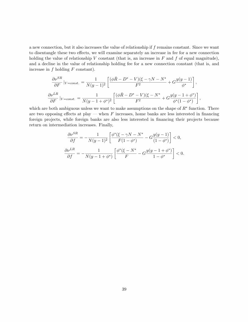
a new connection, but it also increases the value of relationship if f remains constant. Since we wantto disentangle these two effects, we will examine separately an increase in fee for a new connectionholding the value of relationship V constant (that is, an increase in F and f of equal magnitude),and a decline in the value of relationship holding fee for a new connection constant (that is, andincrease in f holding F constant).

∂�SR

∂F∣V=const. =

1

N(y − 1)2

[(�R−D∗ − V )(� − N −N∗

F 2+G

y(y − 1)

�∗

],

∂�LR

∂F∣V=const. =

1

N(y − 1 + �∗)2

[(�R−D∗ − V )(� −N∗

F 2+G

y(y − 1 + �∗)

�∗(1− �∗)

],

which are both ambiguous unless we want to make assumptions on the shape of R∗ function. Thereare two opposing effects at play — when F increases, home banks are less interested in financingforeign projects, while foreign banks are also less interested in financing their projects becausereturn on intermediation increases. Finally,

∂�SR

∂f= − 1

N(y − 1)2

[�∗(� − N −N∗

F (1− �∗)−Gy(y − 1)

(1− �∗)

]< 0,

∂�LR

∂f= − 1

N(y − 1 + �∗)

[�∗(� −N∗

F−Gy(y − 1 + �∗)

1− �∗

]< 0.

39

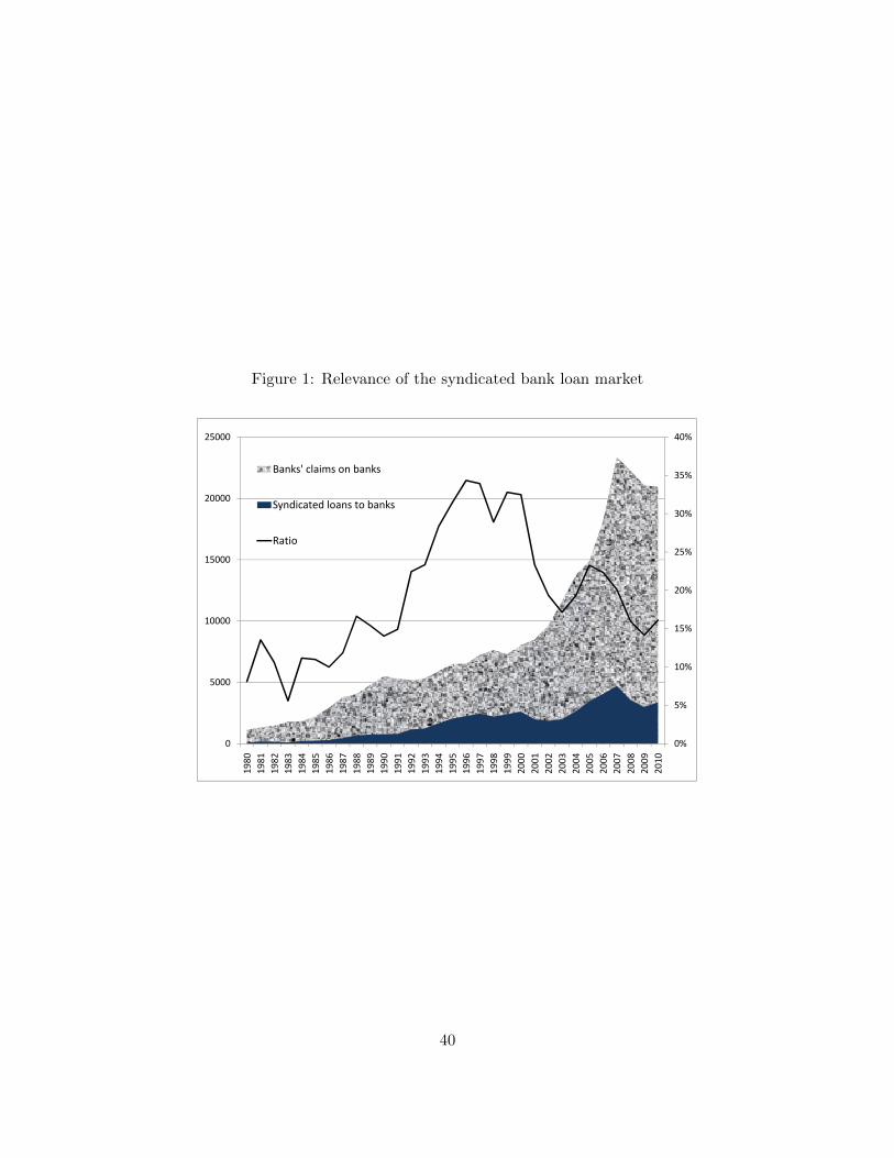
Figure 1: Relevance of the syndicated bank loan market

20%

25%

30%

35%

40%

10000

15000

20000

25000

Banks' claims on banks

Syndicated loans to banks

Ratio

0%

5%

10%

15%

0

5000

1980

1981

1982

1983

1984

1985

1986

1987

1988

1989

1990

1991

1992

1993

1994

1995

1996

1997

1998

1999

2000

2001

2002

2003

2004

2005

2006

2007

2008

2009

2010

40

Figure 2: Network size

Remove density

0

200

400

600

800

1000

1200

1400

1600

1800

2000

0

200

400

600

800

1000

1200

1400

1600

1800

200019

8019

8119

8219

8319

8419

8519

8619

8719

8819

8919

9019

9119

9219

9319

9419

9519

9619

9719

9819

9920

0020

0120

0220

0320

0420

0520

0620

0720

0820

09

Network size: banks

US recessions

Number of new banks

Number of banks

0

1000

2000

3000

4000

5000

6000

7000

0

1000

2000

3000

4000

5000

6000

7000

980

981

982

983

984

985

986

987

988

989

990

991

992

993

994

995

996

997

998

999

000

001

002

003

004

005

006

007

008

009

Network size: connections

US recessions

Number of new connections

Number of connections

00

1980

1981

1982

1983

1984

1985

1986

1987

1988

1989

1990

1991

1992

1993

1994

1995

1996

1997

1998

1999

2000

2001

2002

2003

2004

2005

2006

2007

2008

2009

0

10

20

30

40

50

60

70

80

90

100

0

10

20

30

40

50

60

70

80

90

100

1980

1981

1982

1983

1984

1985

1986

1987

1988

1989

1990

1991

1992

1993

1994

1995

1996

1997

1998

1999

2000

2001

2002

2003

2004

2005

2006

2007

2008

2009

Network size: countries

US recessions

Number of new countries

Number of countries

41

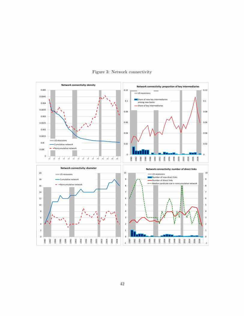
Figure 3: Network connectivity Figre 5: direct.pdf

0

0.0005

0.001

0.0015

0.002

0.0025

0.003

0.0035

0.004

0.0045

0.005

1… 1… 1… 1… 1… 1… 1… 1… 1… 1… 2… 2… 2… 2… 2…

Network connectivity: density

US recessions

Cumulative network

Noncumulative network

0

2

4

6

8

10

12

14

16

18

20

Network connectivity: diameter

US recessions

Cumulative network

Noncumulative network

0

1

2

3

4

5

6

7

8

9

10

0

1

2

3

4

5

6

7

8

9

10

Network connectivity: number of direct links

US recessionsNumber of new direct linksNumber of direct linksMedian syndicate size in noncumulative network

0

0.02

0.04

0.06

0.08

0.1

0.12

0

0.02

0.04

0.06

0.08

0.1

0.12

1980

1982

1984

1986

1988

1990

1992

1994

1996

1998

2000

2002

2004

2006

2008

Network connectivity: proportion of key intermediaries

US recessions

Share of new key intermediaries among new banks

Share of key intermediaries

0

1980

1982

1984

1986

1988

1990

1992

1994

1996

1998

2000

2002

2004

2006

2008

‐1

0

‐1

0

1980

1982

1984

1986

1988

1990

1992

1994

1996

1998

2000

2002

2004

2006

2008

42

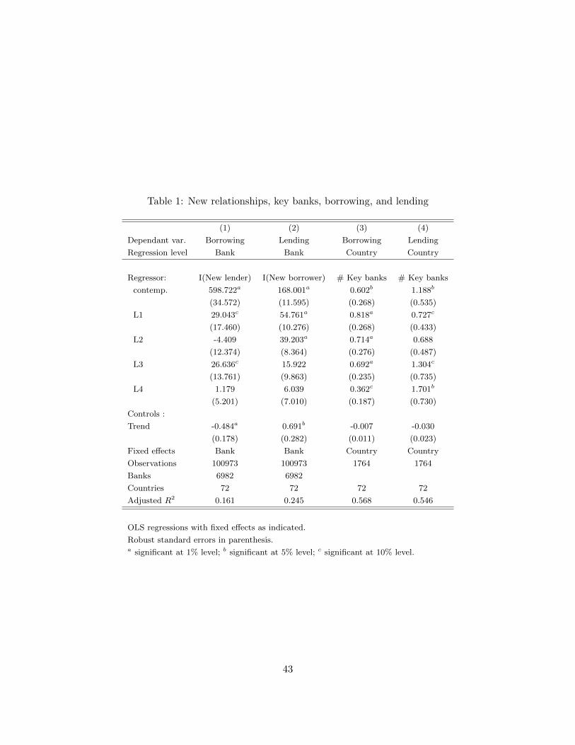
Table 1: New relationships, key banks, borrowing, and lending

(1) (2) (3) (4)

Dependant var. Borrowing Lending Borrowing Lending

Regression level Bank Bank Country Country

Regressor: I(New lender) I(New borrower) # Key banks # Key banks

contemp. 598.722a 168.001a 0.602b 1.188b

(34.572) (11.595) (0.268) (0.535)

L1 29.043c 54.761a 0.818a 0.727c

(17.460) (10.276) (0.268) (0.433)

L2 -4.409 39.203a 0.714a 0.688

(12.374) (8.364) (0.276) (0.487)

L3 26.636c 15.922 0.692a 1.304c

(13.761) (9.863) (0.235) (0.735)

L4 1.179 6.039 0.362c 1.701b

(5.201) (7.010) (0.187) (0.730)

Controls :

Trend -0.484a 0.691b -0.007 -0.030

(0.178) (0.282) (0.011) (0.023)

Fixed effects Bank Bank Country Country

Observations 100973 100973 1764 1764

Banks 6982 6982

Countries 72 72 72 72

Adjusted R2 0.161 0.245 0.568 0.546

OLS regressions with fixed effects as indicated.

Robust standard errors in parenthesis.a significant at 1% level; b significant at 5% level; c significant at 10% level.

43

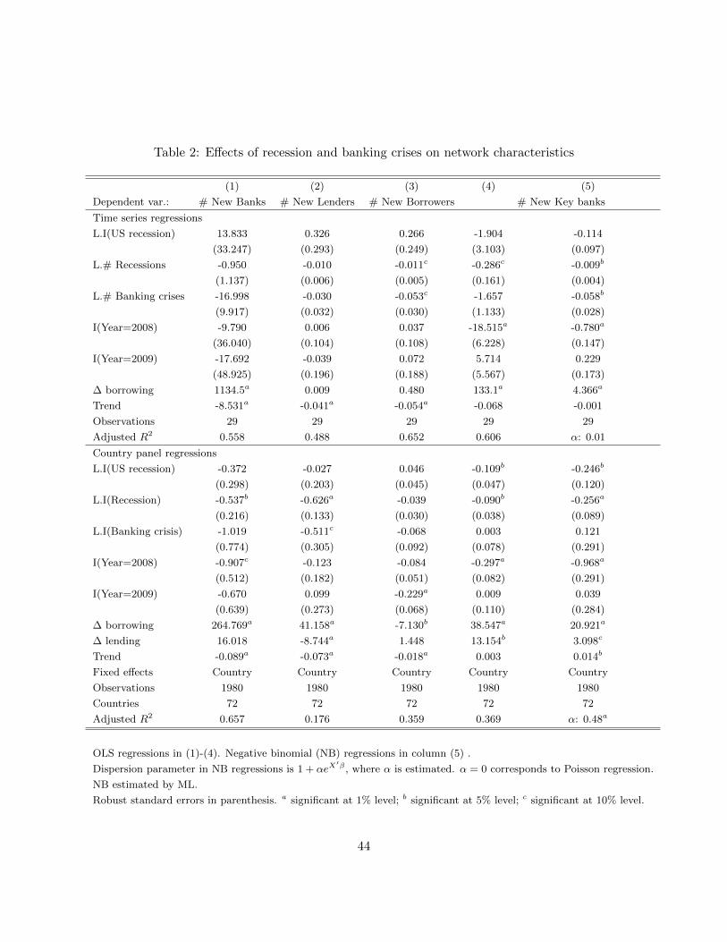
Table 2: Effects of recession and banking crises on network characteristics

(1) (2) (3) (4) (5)

Dependent var.: # New Banks # New Lenders # New Borrowers # New Key banks

Time series regressions

L.I(US recession) 13.833 0.326 0.266 -1.904 -0.114

(33.247) (0.293) (0.249) (3.103) (0.097)

L.# Recessions -0.950 -0.010 -0.011c -0.286c -0.009b

(1.137) (0.006) (0.005) (0.161) (0.004)

L.# Banking crises -16.998 -0.030 -0.053c -1.657 -0.058b

(9.917) (0.032) (0.030) (1.133) (0.028)

I(Year=2008) -9.790 0.006 0.037 -18.515a -0.780a

(36.040) (0.104) (0.108) (6.228) (0.147)

I(Year=2009) -17.692 -0.039 0.072 5.714 0.229

(48.925) (0.196) (0.188) (5.567) (0.173)

Δ borrowing 1134.5a 0.009 0.480 133.1a 4.366a

Trend -8.531a -0.041a -0.054a -0.068 -0.001

Observations 29 29 29 29 29

Adjusted R2 0.558 0.488 0.652 0.606 �: 0.01

Country panel regressions

L.I(US recession) -0.372 -0.027 0.046 -0.109b -0.246b

(0.298) (0.203) (0.045) (0.047) (0.120)

L.I(Recession) -0.537b -0.626a -0.039 -0.090b -0.256a

(0.216) (0.133) (0.030) (0.038) (0.089)

L.I(Banking crisis) -1.019 -0.511c -0.068 0.003 0.121

(0.774) (0.305) (0.092) (0.078) (0.291)

I(Year=2008) -0.907c -0.123 -0.084 -0.297a -0.968a

(0.512) (0.182) (0.051) (0.082) (0.291)

I(Year=2009) -0.670 0.099 -0.229a 0.009 0.039

(0.639) (0.273) (0.068) (0.110) (0.284)

Δ borrowing 264.769a 41.158a -7.130b 38.547a 20.921a

Δ lending 16.018 -8.744a 1.448 13.154b 3.098c

Trend -0.089a -0.073a -0.018a 0.003 0.014b

Fixed effects Country Country Country Country Country

Observations 1980 1980 1980 1980 1980

Countries 72 72 72 72 72

Adjusted R2 0.657 0.176 0.359 0.369 �: 0.48a

OLS regressions in (1)-(4). Negative binomial (NB) regressions in column (5) .

Dispersion parameter in NB regressions is 1 + �eX′� , where � is estimated. � = 0 corresponds to Poisson regression.

NB estimated by ML.

Robust standard errors in parenthesis. a significant at 1% level; b significant at 5% level; c significant at 10% level.

44

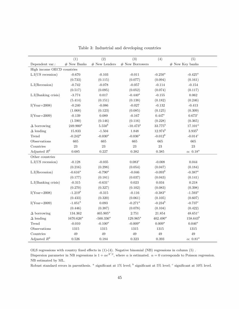
Table 3: Industrial and developing countries

(1) (2) (3) (4) (5)

Dependent var.: # New Banks # New Lenders # New Borrowers # New Key banks

High income OECD countries

L.I(US recession) -0.670 -0.103 -0.011 -0.250a -0.425a

(0.733) (0.115) (0.077) (0.094) (0.161)

L.I(Recession) -0.742 -0.078 -0.057 -0.114 -0.154

(0.517) (0.095) (0.052) (0.074) (0.117)

L.I(Banking crisis) -3.774 0.017 -0.440a -0.155 0.062

(5.414) (0.151) (0.138) (0.182) (0.246)

I(Year=2008) -0.240 -0.086 -0.027 -0.132 -0.413

(1.068) (0.123) (0.085) (0.125) (0.309)

I(Year=2009) -0.139 0.089 -0.167 0.447c 0.673c

(1.590) (0.146) (0.116) (0.228) (0.365)

Δ borrowing 249.900a 5.550b -10.473a 33.775b 17.101a

Δ lending 15.833 -1.504 1.848 12.974b 3.935b

Trend -0.242a -0.030a -0.036a -0.012b -0.014c

Observations 665 665 665 665 665

Countries 23 23 23 23 23

Adjusted R2 0.685 0.227 0.382 0.385 �: 0.18a

Other countries

L.I(US recession) -0.128 -0.035 0.083c -0.008 0.044

(0.216) (0.298) (0.054) (0.047) (0.184)

L.I(Recession) -0.616a -0.790a -0.046 -0.093b -0.387a

(0.177) (0.181) (0.037) (0.043) (0.141)

L.I(Banking crisis) -0.315 -0.631c 0.023 0.034 0.218

(0.270) (0.327) (0.102) (0.083) (0.398)

I(Year=2008) -1.219b -0.315 -0.116 -0.383a -1.593a

(0.433) (0.320) (0.061) (0.105) (0.607)

I(Year=2009) -1.051b 0.093 -0.271a -0.234b -0.737c

(0.446) (0.387) (0.078) (0.104) (0.422)

Δ borrowing 134.362 465.905a 2.751 21.854 48.651c

Δ lending 1670.626a -500.336a 129.965a 402.490a 158.643b

Trend -0.010 -0.100a -0.009a 0.009a 0.046a

Observations 1315 1315 1315 1315 1315

Countries 49 49 49 49 49

Adjusted R2 0.526 0.184 0.323 0.393 �: 0.81a

OLS regressions with country fixed effects in (1)-(4). Negative binomial (NB) regressions in column (5) .

Dispersion parameter in NB regressions is 1 + �eX′� , where � is estimated. � = 0 corresponds to Poisson regression.

NB estimated by ML.

Robust standard errors in parenthesis. a significant at 1% level; b significant at 5% level; c significant at 10% level.

45

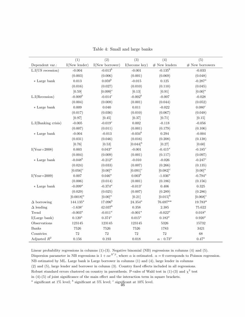
Table 4: Small and large banks

(1) (2) (3) (4) (5)

Dependent var.: I(New lender) I(New borrower) I(become key) # New lenders # New borrowers

L.I(US recession) -0.004 -0.013b -0.001 -0.135b -0.033

(0.003) (0.006) (0.001) (0.069) (0.048)

∗ Large bank 0.013 0.059b -0.015 0.125 -0.287a

(0.016) (0.027) (0.010) (0.110) (0.045)

[0.59] [0.099]c [0.13] [0.91] [0.00]a

L.I(Recession) -0.009b -0.014c -0.002b -0.007 -0.028

(0.004) (0.008) (0.001) (0.044) (0.052)

∗ Large bank 0.009 0.040 0.011 -0.022 0.080c

(0.017) (0.036) (0.010) (0.067) (0.048)

[0.97] [0.45] [0.37] [0.71] [0.15]

L.I(Banking crisis) -0.005 -0.019c 0.002 -0.118 -0.056

(0.007) (0.011) (0.001) (0.179) (0.106)

∗ Large bank -0.004 -0.013 -0.034b 0.294 -0.004

(0.031) (0.046) (0.016) (0.208) (0.138)

[0.76] [0.53] [0.044]b [0.27] [0.60]

I(Year=2008) 0.003 0.043a -0.001 -0.415a -0.185c

(0.004) (0.009) (0.001) (0.117) (0.097)

∗ Large bank -0.048b -0.212a -0.010 -0.026 -0.247c

(0.024) (0.033) (0.007) (0.266) (0.135)

[0.056]c [0.00]a [0.091]c [0.082]c [0.00]a

I(Year=2009) 0.007 0.046a 0.003b -1.036a -0.794a

(0.006) (0.014) (0.001) (0.186) (0.156)

∗ Large bank -0.099a -0.374a -0.013c 0.406 0.325

(0.029) (0.025) (0.007) (0.289) (0.286)

[0.0018]a [0.00]a [0.21] [0.015]b [0.068]c

Δ borrowing 144.135a 17.096b 24.354a 76.697** 19.783*

Δ lending -1.638c 42.037b 0.358 2.385 75.622

Trend -0.003a -0.011a -0.001a -0.022a 0.018a

I(Large bank) 0.120a 0.374a 0.015a 0.182a 0.920a

Observations 123145 123145 123145 5326 15732

Banks 7526 7526 7526 1783 3421

Countries 72 72 72 72 68

Adjusted R2 0.156 0.193 0.018 � : 0.73a 0.47a

Linear probability regressions in columns (1)-(3). Negative binomial (NB) regressions in columns (4) and (5).

Dispersion parameter in NB regressions is 1 + �eX′� , where � is estimated. � = 0 corresponds to Poisson regression.

NB estimated by ML. Large bank is Large borrower in columns (1) and (4), large lender in columns

(2) and (5), large lender and borrower in column (3). Country fixed effects included in all regressions.

Robust standard errors clustered on country in parenthesis. P-vales of Wald test in (1)-(3) and �2 test

in (4)-(5) of joint significance of the main effect and the interaction term in square brackets.a significant at 1% level; b significant at 5% level; c significant at 10% level.

46