Bank of Canada Review · The Bank of Canada Review is published four times a year. Articles undergo a thorough review process. The views expressed in the articles are those of the

Bank of Canada ReviewSpring 2013

ArticlesUnconventional Monetary Policies: Evolving Practices, Their Effects and Potential Costs . . . . . . . . . . . . . . . . . . . 1Eric Santor and Lena Suchanek

Explaining Canada’s Regional Migration Patterns . . . . . . . . . 16David Amirault, Daniel de Munnik and Sarah Miller

Modelling the Asset-Allocation and Liability Strategy for Canada’s Foreign Exchange Reserves . . . . . . . . . . . . . . 29Francisco Rivadeneyra, Jianjian Jin, Narayan Bulusu and Lukasz Pomorski

Members of the Editorial Board

Chair: Allan Crawford

David Beers

Paul Chilcott

Don Coletti

Agathe Côté

Donna Howard

Sharon Kozicki

Timothy Lane

Tiff Macklem

Ron Morrow

John Murray

Sheila Niven

Lawrence Schembri

Evan Siddall

Ianthi Vayid

Richard Wall

Carolyn Wilkins

David Wolf

Editor: Alison Arnot

The Bank of Canada Review is published four times a year. Articles undergo a thorough review process. The views expressed in the articles are those of the authors and do not necessarily reflect the views of the Bank.

The contents of the Review may be reproduced or quoted, provided that the publication, with its date, is specifically cited as the source.

For further information, contact:

Public Information Communications Department Bank of Canada Ottawa, Ontario, Canada K1A 0G9

Telephone: 613 782-8111; 1 800 303-1282 (toll free in North America) Email: [email protected] Website: bankofcanada.ca

ISSN 1483-8303 © Bank of Canada 2013

mailto: [email protected]

http://www.bankofcanada.ca

Unconventional Monetary Policies: Evolving Practices, Their Effects and Potential CostsEric Santor, International Economic Analysis, and Lena Suchanek, Canadian Economic Analysis

� Central banks have introduced several types of unconventional monetary policy measures, ranging from liquidity and credit facilities to asset purchases and forward guidance.

� To date, these measures appear to have been successful. They helped to restore market functioning, facilitated the transmission of monetary policy and supported economic activity.

� Such policies, however, have potential costs, including challenges related to the greatly expanded balance sheets of central banks and the eventual exit from these measures, as well as the vulnerabilities that can arise from prolonged monetary accommodation.

The Great Recession that followed the financial and economic crisis of 2007–09 provoked an unprecedented policy response from central banks, including lowering policy rates to close to zero and employing unconven-tional monetary policy measures.1 Given the weak recovery in the major advanced economies, some central banks have continued to apply these measures.

Most observers agree that unconventional measures have been successful. Liquidity and credit facilities have helped to restore market functioning, repair dysfunctional credit markets and facilitate the transmission of monetary policy. Meanwhile, asset purchases—such as large-scale asset purchases (LSAPs) or quantitative easing (QE)—and forward guidance have supported economic activity and helped central banks to achieve their price-stability objectives. There is, however, a growing awareness of the potential costs and risks associated with (i) the greatly expanded balance sheets of central banks; (ii) the eventual, but unprecedented, exit from unconventional policy measures; and (iii) the vulnerabilities that can arise from an environment of very low policy rates in the major advanced economies for a prolonged period (referred to as “low for long”). Moreover, there is the risk that monetary policy may be trying to address issues that

1 These measures, in particular the provision of liquidity, straddle the line between financial stability policies and monetary policies, facilitating the transmission of monetary policy. We refer to them here as unconventional monetary policy.

The Bank of Canada Review is published four times a year. Articles undergo a thorough review process. The views expressed in the articles are those of the authors and do not necessarily reflect the views of the Bank. The contents of the Review may be reproduced or quoted, provided that the publication, with its date, is specifically cited as the source.

1 UnConvEnTional MonETary PoliCiEs: Evolving PraCTiCEs, ThEir EffECTs and PoTEnTial CosTs BankofCanadaReview•SpRing2013

are better tackled by fiscal or structural reforms. Nevertheless, to date, the benefits of unconventional measures appear to outweigh their potential costs (Bernanke 2012).

This article first summarizes the various types of unconventional monetary policy measures, the channels through which they work and the conse-quences of such policies for central bank balance sheets. This is followed by a discussion of the effectiveness and potential costs of these measures.

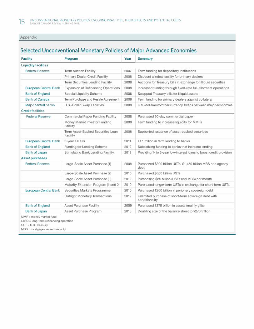
Unconventional Monetary Policies: Evolving PracticesThe types of unconventional monetary policy measures implemented by cen-tral banks have evolved since the onset of the crisis. In this article, we distin-guish between liquidity facilities, credit facilities, asset purchases and forward guidance (see the Appendix on page 15 for a list of selected measures).2

The financial crisis that started in 2007 intensified in September 2008, as liquidity dried up and maturities shortened, leading to an unprecedented increase in spreads (Chart 1). To alleviate financial market disruptions, cen-tral banks quickly provided liquidity to short-term funding markets through a number of emergency facilities and currency swap agreements. They also introduced new or expanded credit facilities, designed to restore the provi-sion of credit in specific markets.

In late 2008, as the impact of the financial crisis spread to the real economy, major central banks lowered policy rates to close to zero. To ease monetary conditions further, many turned to LSAPs. To counter weak aggregate demand, the U.S. Federal Reserve and the Bank of England purchased government debt to put downward pressure on long-term yields.3 The Bank of Japan introduced a more modest purchase program to fight persistent

2 Liquidity facilities involve the provision of liquidity by central banks to address elevated pressures in term funding markets. Credit facilities are measures aimed at restoring the functioning of a particular credit market and promoting bank lending. LSAPs are sizable medium- to long-term asset purchases (mostly of government debt) by the central bank. Forward guidance is central bank communication regarding the future path of the policy rate.

3 The Federal Reserve also purchased mortgage-backed securities and agency debt, as well as long-term securities in exchange for short-term securities (through its Maturity Extension Program).

Note: The LIBOR-OIS spread is the difference between the London Interbank Offered Rate (or equivalent) and the Overnight Index Swap. It is a measure of stress in the money markets.

Sources: Bloomberg and Bank of Canada calculations Last observation: 6 May 2013

Canada United States Euro area United Kingdom

2007 2008 2009 2010 2011 20120

50

100

150

200

250

300

350

400

2013

Basis points

Start of crisis

Bear Stearns rescue

Euro-area debt crisisLehman Brothers bankruptcy

Chart 1: Three-month LIBOR-OIS spreadBasis points, daily data


deflation. Against the backdrop of a euro-area debt crisis, the European Central Bank (ECB) introduced the Securities Markets Programme (SMP), which focused on stabilizing government securities markets to promote the transmission of monetary stimulus.

When global economic growth weakened again in late 2011 through 2013, monetary policy-makers in some advanced economies reintroduced LSAPs, such as the Federal Reserve’s open-ended purchases of Treasuries and mortgage-backed securities. Likewise, in order to achieve its newly stated inflation target of 2 per cent within two years, the Bank of Japan announced in April that it will double its holdings of Japanese government bonds over the next two years.

To reduce long-term interest rates further, some central banks enhanced their guidance on the future path of the policy rate. For example, in April 2009, the Bank of Canada stated, “Conditional on the outlook for inflation, the target overnight rate can be expected to remain at its current level until the end of the second quarter of 2010 in order to achieve the inflation target.”4 The Federal Reserve first introduced date-based guidance in 2011 and then outcome-based guidance in 2012, in which the future path of the federal funds rate was tied to explicit outcomes in the unemployment rate and inflation.

In addition, as the flow of credit through the banking system remained impaired, both the Bank of England and the Bank of Japan introduced finan-cing schemes to promote lending by banks to households and businesses, while the ECB extended the maturity and quantity of lending to banks in the euro area through its long-term refinancing operations (LTROs).5

To sum up, central banks reacted in a timely and aggressive manner to the financial and economic crisis, implementing a variety of unconventional meas-ures, and tailoring the type and magnitude of the measures to domestic market conditions. As conditions evolved, so did the approaches taken by central banks; they extended existing policies and introduced new ones in order to achieve their objectives for monetary policy and financial stability.

Channels of Unconventional Monetary PolicyUnconventional monetary policy affects financial markets and the economy more broadly through several channels. Liquidity facilities work directly on the targeted markets, but also have wider effects, such as enhancing the viability of banks by preventing a liquidity crisis from becoming a solvency crisis and improving the transmission of monetary policy. Likewise, credit facilities, such as the ECB’s LTROs, increase the ability of banks to provide credit to the real economy and support the sovereign debt market, while other credit facilities, such as the Federal Reserve’s Commercial Paper Funding Facility, revive specific credit markets through the purchase of assets. LSAPs work through multiple channels, both directly and indirectly, by:

(i) increasing the prices of the purchased assets, thereby lowering their yield, and creating wealth effects that in turn support consumption;

(ii) motivating investors to rebalance their portfolios toward higher-return, riskier assets;

4 The Bank of Canada was less aggressive than most of its advanced-economy counterparts in its use of unconventional policies, reflecting the resilience of the Canadian financial system and its strong underlying macroeconomic policy framework.

5 The LTROs also helped support the sovereign debt market, as banks used borrowed liquidity to buy government bonds, especially in the euro-area periphery.

Central banks tailored the type and magnitude of unconventional measures to domestic market conditions


(iii) providing a signal about the future path of the policy rate;

(iv) putting downward pressure on the exchange rate;

(v) better anchoring inflation expectations, leading to lower real interest rates; and

(vi) demonstrating that the central bank is willing to do whatever it takes to meet its objectives, thus supporting confidence.

Forward guidance works by influencing market participants’ expectations of the future path of the policy rate and the term structure of interest rates. Specifically, if the central bank credibly communicates that the policy rate will likely remain lower for a longer period than previously indicated, this will serve to lower long-term interest rates as well, which will affect the economy in ways similar to those described for LSAPs.

Central Bank Balance SheetsThe measures taken by many central banks have had significant implica-tions for the size and composition of their balance sheets. Stated as a per-centage of gross domestic product (GDP), the balance sheets of the Federal Reserve and the ECB have more than doubled since 2007, and the Bank of England’s has quadrupled (Chart 2).6 The Bank of Japan’s balance sheet has increased by only 50 per cent so far, but, under its recently announced policy, it is expected to increase to approximately 60 per cent of GDP by the end of 2014. While purchases of government debt (and mortgage securities) account for the bulk of this expansion for most countries, LTROs repre-sented most of the increase in the ECB’s balance sheet.

In terms of composition, the average maturity of central banks’ port-folios has often lengthened and their risk profile has increased, owing to new practices such as purchasing riskier assets and relaxing collateral

6 In contrast, the Bank of Canada’s balance sheet increased by only about 50 per cent from 2007 to 2009, before falling back to close to its previous level as a share of GDP.

The measures taken by many central banks have had significant implications for the size and composition of their balance sheets

Units of measure (top of axis):

Verifi ed vs. supplied data, cross-referenced w/ prior artwork

Left alt scale, if applicable

Aligned to outer edgeof axis labels, rag inward towards chart

Chart axes:

Tick marks (major and, if necessary, minor)

“Bookend” tick marks at ends of bottom axis (left/right)

Bottom axis labels placed & verifi ed

Chart bottom region:

Legend items placed and styled

Order verifi ed vs prior artwork

All superscripts, special symbols, etc. as required

Chart footer:

Note(s):

Source(s):

Last observation: (if applicable)

Data presentation styles:

Line styles & stacking order:

Canada/1st

US/2nd

Euro zone/3rd

Japan/4th

UK/5th

Canada/1st (projected)

US/2nd (proj’d)

Euro zone/3rd (proj’d)

Japan/4th (proj’d)

UK/5th (proj’d)

All axis lines & ticks

Fill styles & stacking order:

Canada/1st

US/2nd

Euro zone/3rd

Japan/4th UK/5th projected


US/2nd (proj’d)



UK/5th (proj’d)

Control range

Axis lines & ticks

Additional common styles:

dot black

red line plus dot in-chart label

Chart 1: Title+ 2nd line

Sub-title

Sources: U.S. Federal Reserve, U.S. Bureau of Economic Analysis;Bank of England, U.K. Offi ce for National Statistics; European Last observations:Central Bank, Eurostat; Bank of Japan, Cabinet Offi ce of Japan; and United States, 2013Q1;Bank of Canada calculations all others, 2012Q4

Bank of Canada U.S. Federal Reserve

Bank of England European Central Bank

Bank of Japan

2007 2008 2009 2010 2011 2012

0

5

10

15

20

25

30

35

%

Chart 2: Total assets on central bank balance sheetsAs a percentage of GDP, quarterly data


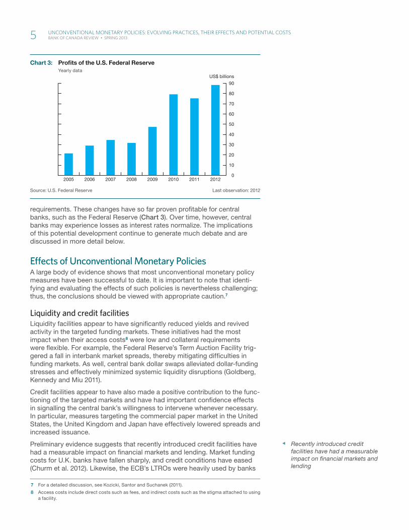
requirements. These changes have so far proven profitable for central banks, such as the Federal Reserve (Chart 3). Over time, however, central banks may experience losses as interest rates normalize. The implications of this potential development continue to generate much debate and are discussed in more detail below.

Effects of Unconventional Monetary PoliciesA large body of evidence shows that most unconventional monetary policy measures have been successful to date. It is important to note that identi-fying and evaluating the effects of such policies is nevertheless challenging; thus, the conclusions should be viewed with appropriate caution.7

Liquidity and credit facilitiesLiquidity facilities appear to have significantly reduced yields and revived activity in the targeted funding markets. These initiatives had the most impact when their access costs8 were low and collateral requirements were flexible. For example, the Federal Reserve’s Term Auction Facility trig-gered a fall in interbank market spreads, thereby mitigating difficulties in funding markets. As well, central bank dollar swaps alleviated dollar-funding stresses and effectively minimized systemic liquidity disruptions (Goldberg, Kennedy and Miu 2011).

Credit facilities appear to have also made a positive contribution to the func-tioning of the targeted markets and have had important confidence effects in signalling the central bank’s willingness to intervene whenever necessary. In particular, measures targeting the commercial paper market in the United States, the United Kingdom and Japan have effectively lowered spreads and increased issuance.

Preliminary evidence suggests that recently introduced credit facilities have had a measurable impact on financial markets and lending. Market funding costs for U.K. banks have fallen sharply, and credit conditions have eased (Churm et al. 2012). Likewise, the ECB’s LTROs were heavily used by banks

7 For a detailed discussion, see Kozicki, Santor and Suchanek (2011).

8 Access costs include direct costs such as fees, and indirect costs such as the stigma attached to using a facility.

Recently introduced credit facilities have had a measurable impact on financial markets and lending

Source: U.S. Federal Reserve Last observation: 2012

2005 2006 2007 2008 2009 2010 2011 20120

10

20

30

40

50

60

70

80

90

US$ billions

Chart 3: Profi ts of the U.S. Federal ReserveYearly data


and triggered an important decline in interest rate premiums, reduced sys-temic risk, led to lower yield spreads for peripheral sovereigns and likely mitigated a credit crunch in the euro area. Moreover, market sentiment improved and previously closed bank funding markets gradually reopened (ECB 2012a).

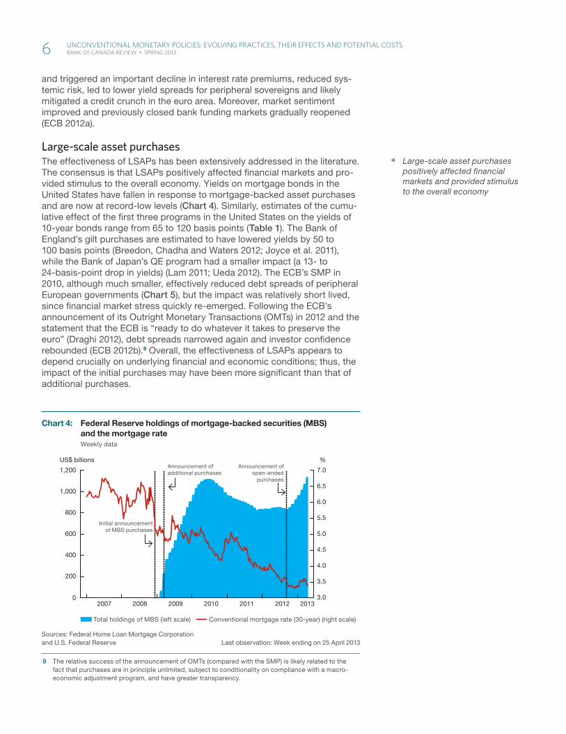
Large-scale asset purchasesThe effectiveness of LSAPs has been extensively addressed in the literature. The consensus is that LSAPs positively affected financial markets and pro-vided stimulus to the overall economy. Yields on mortgage bonds in the United States have fallen in response to mortgage-backed asset purchases and are now at record-low levels (Chart 4). Similarly, estimates of the cumu-lative effect of the first three programs in the United States on the yields of 10-year bonds range from 65 to 120 basis points (Table 1). The Bank of England’s gilt purchases are estimated to have lowered yields by 50 to 100 basis points (Breedon, Chadha and Waters 2012; Joyce et al. 2011), while the Bank of Japan’s QE program had a smaller impact (a 13- to 24-basis-point drop in yields) (Lam 2011; Ueda 2012). The ECB’s SMP in 2010, although much smaller, effectively reduced debt spreads of peripheral European governments (Chart 5), but the impact was relatively short lived, since financial market stress quickly re-emerged. Following the ECB’s announcement of its Outright Monetary Transactions (OMTs) in 2012 and the statement that the ECB is “ready to do whatever it takes to preserve the euro” (Draghi 2012), debt spreads narrowed again and investor confidence rebounded (ECB 2012b).9 Overall, the effectiveness of LSAPs appears to depend crucially on underlying financial and economic conditions; thus, the impact of the initial purchases may have been more significant than that of additional purchases.

9 The relative success of the announcement of OMTs (compared with the SMP) is likely related to the fact that purchases are in principle unlimited, subject to conditionality on compliance with a macro-economic adjustment program, and have greater transparency.

Large-scale asset purchases positively affected financial markets and provided stimulus to the overall economy

Sources: Federal Home Loan Mortgage Corporation and U.S. Federal Reserve Last observation: Week ending on 25 April 2013

Total holdings of MBS (left scale) Conventional mortgage rate (30-year) (right scale)

2007 2008 2009 2010 2011 2012 2013

%

200

400

600

800

3.0

3.5

4.0

4.5

5.0

5.5

6.0

6.5

7.01,200

1,000

US$ billions

0

Initial announcementof MBS purchases

Announcement of additional purchases

Announcement of open-ended

purchases

Chart 4: Federal Reserve holdings of mortgage-backed securities (MBS) and the mortgage rateWeekly data


Research suggests that, in addition to their impact on financial markets, the LSAPs in the United States have provided meaningful support to the economic recovery and have contributed to the achievement of price sta-bility (in part by helping to prevent disinflation or even deflation) (Table 1). The evidence for the Bank of England’s QE program is similar, suggesting a peak effect of 1 1/2 to 2 per cent for real output and between 3/4 and 1 1/2 per cent for inflation (Joyce, Tong and Woods 2011). Overall, LSAPs appear to have been effective when the total stock purchased relative to the size of the target market was large, and when their terms and objectives were transparently and clearly communicated.

Table 1: Impact of large-scale asset purchases in the United States

Total size (US$ billions)

Impact on

Treasury yields Level of GDP

basis points

basis points per

US$100 billion %% per

US$100 billion

LSAP1

Range of estimates 1,750 38 to 107a 2.2 to 6.1a 0.7 to 3b 0.04 to 0.17b

Bernanke (2012) 1,750 40 to 110 2.3 to 6.3

LSAP2

Range of estimates 600 13 to 45c 2.2 to 7.5c 0.4 to 1d 0.07 to 0.17d

Bernanke (2012) 600 15 to 45 2.5 to 7.5

LSAP1 + LSAP2

Bernanke (2012) 2,350 3 0.13

LSAP1 + LSAP2 + Maturity Extension Program

Range of estimates 2,750 65 to 100e 2.4 to 3.6e

Bernanke (2012) 2,750 80 to 120 2.9 to 4.4

a. Ihrig et al. 2012; Doh 2010; Meyer and Bomfi m 2010; Gagnon et al. 2011; Neely 2012 b. Chung et al. 2012; Deutsche Bank 2010; Baumeister and Benati 2010c. Ihrig et al. 2012; Krishnamurthy and Vissing-Jorgensen 2011; D’Amico et al. 2012d. Chen, Cúrdia and Ferrero 2012; Chung et al. 2012; Meyer and Bomfi m 2011e. Ihrig et al. 2012; Li and Wei 2012; Meyer and Bomfi m 2012

Note: Owing to data limitations, an 8-year generic bond is used for Ireland. A generic x-year bond is the bond that has the closest maturity to x at any given point in time.

Sources: Bloomberg and Bank of Canada calculations Last observation: 6 May 2013

Greece (left scale) Spain Portugal Italy Ireland

Chart 5: Euro-area periphery 10-year generic bond spreadsPercentage-point difference in yields of generic German bonds, daily data

2010 2011 2012 20130

2

4

6

8

10

12

14

16

%

0

5

10

15

20

25

30

35

%

Securities Markets Programme

Long-term refi nancing operations

Outright Monetary Transactions


Forward guidanceThe Federal Reserve’s experience with forward guidance appears to have been successful. Since the Federal Reserve’s extension of its commitment regarding the federal funds rate, market participants have pushed back the date at which they expect the rate to begin to rise. This response is evident in the reaction of financial market prices and in survey data (Bernanke 2012). The Bank of Canada’s conditional commitment also succeeded in changing market expectations. Yield-curve expectations declined after the Bank’s announcement, strengthening the rebound in growth and inflation in Canada (Carney 2012).10

While unconventional policies appear to have achieved their objectives to date, it is too early to judge the overall success of such practices, since it remains unclear how well central banks will exit from these policies.

Policy Issues and Potential CostsTo date, there is little hard analysis of the potential costs of unconventional monetary policies. Nevertheless, central banks need to consider a number of issues when pursuing such policies.

Exit and balance-sheet managementA vibrant debate is emerging on the issue of the exit from unconventional monetary policies. Exiting too soon could undermine the recovery, while too slow an exit could lead to excess liquidity and contribute to inflationary pressures. Clear communication and guidance will be crucial for a suc-cessful exit.

Despite the expansion in the monetary base relative to the economy (Chart 6), to date, inflation has largely been in line with the price-stability objectives of major central banks (Chart 7), and inflation expectations remain generally well anchored.11 Nevertheless, the increased liquidity in the financial system needs to be managed appropriately to avoid future infla-tionary pressures.

The degree of monetary policy accommodation can be reduced by raising the target for the overnight rate and the interest paid on reserves,12 by imple-menting reverse repos and by reducing asset holdings on the central bank’s balance sheet (either through asset sales or simply by not rolling over the assets and allowing them to mature). Concurrently raising policy rates and draining reserves may, however, alter the usual transmission mechanism, and so the central bank will need to monitor the process closely (Kozicki, Santor and Suchanek 2011).

Expanded balance sheets expose central banks to potential losses. Recent analysis shows, for example, that the Federal Reserve could experience losses under certain scenarios for asset sales and market interest rates (Carpenter et al. 2013). Moreover, capital losses could result from acquiring riskier assets and relaxing collateral requirements for central bank loans.13

10 For an empirical analysis of the effectiveness of Canada’s conditional commitment policy, see He (2010).

11 Indeed, the expansionary monetary policy stance has not been inflationary because it has com-pensated for a contraction in private credit and private sector deleveraging that would otherwise be deflationary.

12 The higher the interest rate paid on reserves, the lower the incentive for the bank to lend its funds to other banks or to the real economy.

13 The ECB set aside more than half of its interest income for risk provisions in 2012 to account for potential losses on its holdings of government bonds under the SMP.

Exiting from unconventional monetary policies too soon could undermine the recovery, while too slow an exit could lead to excess liquidity and contribute to inflationary pressures


Central banks can, in principle, bear the risks of losses on their balance sheets without impairing their ability to conduct monetary policy.14 In this context, losses would not prevent the central bank from tightening as the real economy begins to improve, since they are a minor cost compared with the larger benefit of better economic growth.

14 In the United States, cumulative earnings over the entire period of unconventional monetary policy actions are estimated to be positive and even higher than they would have been without the LSAPs (Carpenter et al. 2013).

Sources: Bank of Canada, Statistics Canada; Haver Analytics for data from the U.S. Federal Reserve, U.S. Bureau of Economic Analysis, Bank of England, U.K. Offi ce for National Statistics, Last observations:European Central Bank, Eurostat, Bank of Japan and United States, 2013Q1;Cabinet Offi ce of Japan; and Bank of Canada calculations all others, 2012Q4

Canada (left scale) United States United Kingdom Euro area Japan

2006 2007 2008 2009 2010 2011 2012 20130

5

10

15

20

25

25

26

27

28

29

30

31

32

RatioRatio RatioRatio

Chart 6: Ratio of nominal GDP to the monetary baseSeasonally adjusted quarterly data

Note: The core PCE index is used for U.S. data.

Sources: Statistics Canada; and Haver Analytics for data from the U.S. Bureau of Economic Analysis, U.K. Offi ce for National Statistics, Eurostat, and the Ministry of Internal Affairs and Communications of Japan Last observation: 2013Q1

Canada United States United Kingdom Euro area Japan

2008 2009 2010 2011 2012 2013-2

-1

0

1

2

3

4

%

Chart 7: Core CPI in major advanced economiesYear-over-year change, percentage points, seasonally adjusted quarterly data


Central bank independence and credibilityAsset purchases of government debt could undermine the credibility of the central bank if such purchases are seen to be facilitating large fiscal deficits. This could lead to a loss of perceived independence and thus an un-anchoring of inflation expectations. As well, the central bank’s reputation could be damaged should it incur losses on its portfolio. Central banks must therefore ensure that any unconventional policy measures they implement are clearly communicated and aimed squarely at achieving their mandated objectives, and nothing more.

Low for long and financial stabilityIn many countries, the implementation of balance-sheet policies has led to an extended period of very low interest rates across the entire term structure, causing concerns about “low for long” (Carney 2010). For example, institu-tions, such as insurance companies and pension funds, are required—or prefer—to hold long-term assets as part of their portfolios. Given their need to match the returns from such assets with their long-term liabilities, these institutions may feel compelled to invest in riskier assets or implement new business strategies where the risks are not understood as well. More broadly, while portfolio rebalancing is a key channel through which LSAPs work, it could lead to excessive risk taking and increase vulnerabilities in the financial system, requiring heightened diligence on the part of financial supervisors. Finally, “low for long” may lead to forbearance, as loans are extended at low rates that allow otherwise non-viable firms and/or banks to continue oper-ating. These “zombie” firms/banks would impede the needed restructuring of the economy.

Distributional effectsRelated to “low for long” is the concern that asset purchases might have distributional effects; that is, they would benefit one group at the expense of another.15 While lower long-term yields favour borrowers over savers, some observers have argued that the wealth effects associated with portfolio rebalancing would benefit holders of equities over bondholders. Recent analysis suggests that this concern may be overstated, since lower yields are mostly offset by higher asset prices (Bank of England 2012). Nevertheless, central banks should be mindful of distributional effects.

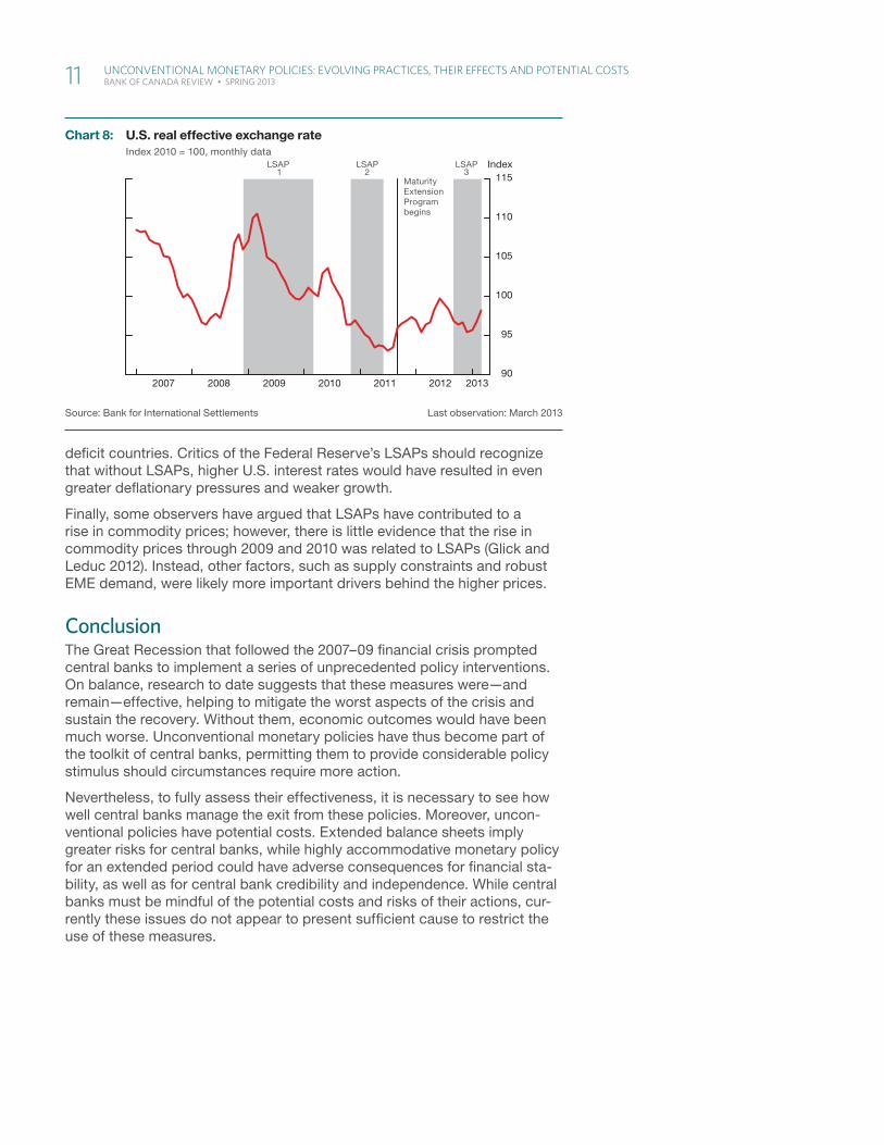
SpilloversMuch like conventional monetary policy, unconventional policies can affect other asset-market prices. Neely (2012) finds that LSAP announcements substantially reduced not only yields on foreign long-term bonds but also the spot value of the U.S. dollar (Chart 8).

Many emerging-market economies (EMEs), and some advanced economies, have criticized the Federal Reserve’s LSAPs as targeting currency deprecia-tion, thereby fuelling capital flows to EMEs. Current research, however, does not support this assertion.16 Moreover, in an environment of deficient demand, LSAPs have proven to be necessary to enable the Federal Reserve to achieve its price-stability objectives. Currency depreciation is part of monetary policy transmission and, in fact, assists in the adjustment process between surplus countries (which would otherwise experience inflation) and

15 While all monetary policy actions are taken for the benefit of the entire economy, such actions will nevertheless have unavoidable distributional effects.

16 See, for example, Ghosh et al. (2012), IMF (2011), and Forbes and Warnock (2012).

Central banks must ensure that any unconventional policy measures they implement are clearly communicated and aimed squarely at achieving their mandated objectives

Much like conventional monetary policy, unconventional policies can affect other asset-market prices


deficit countries. Critics of the Federal Reserve’s LSAPs should recognize that without LSAPs, higher U.S. interest rates would have resulted in even greater deflationary pressures and weaker growth.

Finally, some observers have argued that LSAPs have contributed to a rise in commodity prices; however, there is little evidence that the rise in commodity prices through 2009 and 2010 was related to LSAPs (Glick and Leduc 2012). Instead, other factors, such as supply constraints and robust EME demand, were likely more important drivers behind the higher prices.

ConclusionThe Great Recession that followed the 2007–09 financial crisis prompted central banks to implement a series of unprecedented policy interventions. On balance, research to date suggests that these measures were—and remain—effective, helping to mitigate the worst aspects of the crisis and sustain the recovery. Without them, economic outcomes would have been much worse. Unconventional monetary policies have thus become part of the toolkit of central banks, permitting them to provide considerable policy stimulus should circumstances require more action.

Nevertheless, to fully assess their effectiveness, it is necessary to see how well central banks manage the exit from these policies. Moreover, uncon-ventional policies have potential costs. Extended balance sheets imply greater risks for central banks, while highly accommodative monetary policy for an extended period could have adverse consequences for financial sta-bility, as well as for central bank credibility and independence. While central banks must be mindful of the potential costs and risks of their actions, cur-rently these issues do not appear to present sufficient cause to restrict the use of these measures.

Source: Bank for International Settlements Last observation: March 2013

2007 2008 2009 2010 2011 2012 201390

95

100

105

110

115IndexLSAP

1LSAP

2Maturity Extension Program begins

LSAP3

Chart 8: U.S. real effective exchange rateIndex 2010 = 100, monthly data


Literature CitedBank of England. 2012. “The Distributional Effects of Asset Purchases.”

Bank of England Quarterly Bulletin (Q3): 254–66.

Baumeister, C. and L. Benati. 2010. “Unconventional Monetary Policy and the Great Recession: Estimating the Impact of a Compression in the Yield Spread at the Zero Lower Bound.” European Central Bank Working Paper No. 1258.

Bernanke, B. S. 2012. “Monetary Policy Since the Onset of the Crisis.” Speech at the Federal Reserve Bank of Kansas City Economic Symposium, Jackson Hole, Wyoming, 31 August.

Breedon, F., J. S. Chadha and A. Waters. 2012. “The Financial Market Impact of U.K. Quantitative Easing.” Oxford Review of Economic Policy 28 (4): 702–28.

Carney, M. 2010. “Living with Low for Long.” Speech to the Economic Club of Canada, Toronto, Ontario, 13 December.

—. 2012. “Guidance.” Speech to the CFA Society Toronto, Toronto, Ontario, 11 December.

Carpenter, S. B., J. E. Ihrig, E. C. Klee, D. W. Quinn and A. H. Boote. 2013. “The Federal Reserve’s Balance Sheet and Earnings: A Primer and Projections.” Federal Reserve Board Finance and Economics Discussion Series No. 2013-01.

Chen, H., V. Cúrdia and A. Ferrero. 2012. “The Macroeconomic Effects of Large‐Scale Asset Purchase Programmes.” The Economic Journal 122 (564): F289–F315.

Chung, H., J.-P. Laforte, D. Reifschneider and J. C. Williams. 2012. “Have We Underestimated the Likelihood and Severity of Zero Lower Bound Events?” Journal of Money, Credit and Banking 44 (s1): 47–82.

Churm, R., A. Radia, J. Leake, S. Srinivasan and R. Whisker. 2012. “The Funding for Lending Scheme.” Bank of England Quarterly Bulletin (Q4): 306–20.

D’Amico, S., W. English, D. López-Salido and E. Nelson. 2012. “The Federal Reserve’s Large-Scale Asset Purchase Programmes: Rationale and Effects.” The Economic Journal 122 (564): F415–46.

Deutsche Bank. 2010. “Benefits and Costs of QE2.” Global Economic Perspectives, 29 September.

Doh, T. 2010. “The Efficacy of Large-Scale Asset Purchases at the Zero Lower Bound.” Federal Reserve Board of Kansas City Economic Review (Second Quarter): 5–34.

Draghi, M. 2012. “Verbatim of the Remarks Made by Mario Draghi.” Speech at the Global Investment Conference, London, 26 July.


European Central Bank (ECB). 2012a. “Impact of the Two Three-Year Longer-Term Refinancing Operations.” European Central Bank Monthly Bulletin (March): 37–39.

—. 2012b. Financial Stability Review (December).

Forbes, K. J. and F. E. Warnock. 2012. “Capital Flow Waves: Surges, Stops, Flight and Retrenchment.” Journal of International Economics 88 (2): 235–51.

Gagnon, J., M. Raskin, J. Remache and B. Sack. 2011. “The Financial Market Effects of the Federal Reserve’s Large-Scale Asset Purchases.” International Journal of Central Banking 7 (1): 3–43.

Ghosh, A. R., J. Kim, M. S. Qureshi and J. Zalduendo. 2012. “Surges.” International Monetary Fund Working Paper No. WP/12/22.

Glick, R. and S. Leduc. 2012. “Central Bank Announcements of Asset Purchases and the Impact on Global Financial and Commodity Markets.” Journal of International Money and Finance 31 (8): 2078–101.

Goldberg, L. S., C. Kennedy and J. Miu. 2011. “Central Bank Dollar Swap Lines and Overseas Dollar Funding Costs.” Federal Reserve Bank of New York Economic Policy Review (May): 3–20.

He, Z. 2010. “Evaluating the Effect of the Bank of Canada’s Conditional Commitment Policy.” Bank of Canada Discussion Paper No. 2010-11.

Ihrig, J., E. Klee, C. Li, B. Schulte and M. Wei. 2012. “Expectations About the Federal Reserve’s Balance Sheet and the Term Structure of Interest Rates.” Federal Reserve Board Finance and Economics Discussion Series No. 2012-57.

International Monetary Fund (IMF). 2011. “Recent Experiences in Managing Capital Inflows—Cross-Cutting Themes and Possible Policy Framework.” Strategy, Policy and Review Department (14 February).

Joyce, M., A. Lasaosa, I. Stevens and M. Tong. 2011. “The Financial Market Impact of Quantitative Easing in the United Kingdom.” International Journal of Central Banking 7 (3): 113–61.

Joyce, M., M. Tong and R. Woods. 2011. “The United Kingdom’s Quantitative Easing Policy: Design, Operation and Impact.” Bank of England Quarterly Bulletin (Q3): 200–12.

Kozicki, S., E. Santor and L. Suchanek. 2011. “Unconventional Monetary Policy: The International Experience with Central Bank Asset Purchases.” Bank of Canada Review (Spring): 13–25.

Krishnamurthy, A. and A. Vissing-Jorgensen. 2011. “The Effects of Quantitative Easing on Interest Rates: Channels and Implications for Policy.” Brookings Papers on Economic Activity (Fall): 215–87.

Lam, W. R. 2011. “Bank of Japan’s Monetary Easing Measures: Are They Powerful and Comprehensive?” International Monetary Fund Working Paper No. WP/11/264.


Li, C. and M. Wei. 2012. “Term Structure Modelling with Supply Factors and the Federal Reserve’s Large Scale Asset Purchase Programs.” Federal Reserve Board Finance and Economics Discussion Series No. 2012-37.

Meyer, L. H. and A. N. Bomfim. 2010. “Quantifying the Effects of Fed Asset Purchases on Treasury Yields.” Macroeconomic Advisers, Monetary Policy Insights: Fixed Income Focus, 17 June.

—. 2011. “The Macro Effects of LSAPs II: A Comparison of Three Studies.” Macroeconomic Advisers, Monetary Policy Insights, Policy Focus, 7 February.

—. 2012. “Not Your Father’s Yield Curve: Modeling the Impact of QE on Treasury Yields.” Macroeconomic Advisers, Monetary Policy Insights: Fixed Income Focus, 7 May.

Neely, C. J. 2012. “The Large-Scale Asset Purchases Had Large International Effects.” Federal Reserve Bank of St. Louis Working Paper No. 2010-018D.

Ueda, K. 2012. “The Effectiveness of Non-Traditional Monetary Policy Measures: The Case of the Bank of Japan.” Japanese Economic Review 63 (1): 1–22.


Appendix

Selected Unconventional Monetary Policies of Major Advanced EconomiesFacility Program Year Summary

Liquidity facilities

Federal Reserve Term Auction Facility 2007 Term funding for depository institutions

Primary Dealer Credit Facility 2008 Discount window facility for primary dealers

Term Securities Lending Facility 2008 Auctions for Treasury bills in exchange for illiquid securities

European Central Bank Expansion of Refi nancing Operations 2008 Increased funding through fi xed-rate full-allotment operations

Bank of England Special Liquidity Scheme 2008 Swapped Treasury bills for illiquid assets

Bank of Canada Term Purchase and Resale Agreement 2008 Term funding for primary dealers against collateral

Major central banks U.S.-Dollar Swap Facilities 2008 U.S.-dollar/euro/other currency swaps between major economies

Credit facilities

Federal Reserve Commercial Paper Funding Facility 2008 Purchased 90-day commercial paper

Money Market Investor Funding Facility

2008 Term funding to increase liquidity for MMFs

Term Asset-Backed Securities Loan Facility

2008 Supported issuance of asset-backed securities

European Central Bank 3-year LTROs 2011 €1.1 trillion in term lending to banks

Bank of England Funding for Lending Scheme 2012 Subsidizing funding to banks that increase lending

Bank of Japan Stimulating Bank Lending Facility 2012 Providing 1- to 3-year low-interest loans to boost credit provision

Asset purchases

Federal Reserve Large-Scale Asset Purchase (1) 2008 Purchased $300 billion USTs, $1,450 billion MBS and agency debt

Large-Scale Asset Purchase (2) 2010 Purchased $600 billion USTs

Large-Scale Asset Purchase (3) 2012 Purchasing $85 billion (USTs and MBS) per month

Maturity Extension Program (1 and 2) 2010 Purchased longer-term USTs in exchange for short-term USTs

European Central Bank Securities Markets Programme 2010 Purchased €200 billion in periphery sovereign debt

Outright Monetary Transactions 2012 Unlimited purchase of short-term sovereign debt with conditionality

Bank of England Asset Purchase Facility 2009 Purchased £375 billion in assets (mainly gilts)

Bank of Japan Asset Purchase Program 2013 Doubling size of the balance sheet to ¥270 trillion

MMF = money market fundLTRO = long-term refi nancing operationUST = U.S. Treasury MBS = mortgage-backed security


Explaining Canada’s regional Migration PatternsDavid Amirault, Daniel de Munnik and Sarah Miller, Canadian Economic Analysis

� Understanding the factors that determine the migration of labour between regions is crucial for assessing the response of the economy to macro-economic shocks and identifying policies that will encourage an efficient reallocation of labour.

� Using a gravity model and census data for sub-provincial economic regions, this article examines the determinants of migration within Canada from 1991 to 2006 (the latest available census data). The inclu-sion of intraprovincial data provides a clearer perspective on the migra-tion choices of Canadians than found in previous studies done at the provincial level.

� This research provides evidence that labour migration tends to increase with regional differences in employment rates and household incomes, and that provincial borders and language differences are barriers to migration.

In Canada, as in other small, open, commodity-producing economies with a flexible exchange rate, shocks to the terms of trade (the ratio of export prices to import prices) can cause significant regional variations in output and labour market conditions, because resource-based and manufacturing activities are unevenly distributed across the country (Lefebvre and Poloz 1996). The movement of labour from regions with excess supply to regions with excess demand in response to these and other shocks is an important macroeconomic adjustment mechanism. If this movement is efficient and unencumbered, monetary policy-makers do not need to respond as aggressively to shocks to stabilize prices and the economy. Furthermore, improvements in the efficiency of this adjustment mechanism could help to counteract future expected weak trend growth in labour supply (which is a function of the aging of the population)1 and weak trend growth in productivity,2 and therefore support Canada’s potential output growth.

1 Macklem (2012) suggests that efforts to reduce barriers to interprovincial migration are important elements in a broad strategy to deal with limited growth in the supply of labour in coming years. Examples of current initiatives include the New West Partnership Trade Agreement and the Agreement on Internal Trade.

2 Leung and Cao (2009) report that the higher rates of reallocation within sectors are associated with stronger productivity growth (consistent with models of creative destruction). It therefore follows that the barriers to regional migration may impair sectoral mobility and can result in weaker productivity growth.


16 ExPlaining Canada’s rEgional MigraTion PaTTErns BankofCanadaReview•SpRing2013

This article highlights the patterns of gross aggregate migration across economic regions of Canada and provides evidence of the factors that drive them. It begins with a discussion of insights obtained from previous research and the recent trends reflected in the data. It then describes a basic gravity model of migration (Box 1), and its three core explanatory variables: the respective populations of the two regions sharing the migrants in question plus the distance between the two regions. We extend this framework to include a rich set of additional explanatory variables related to economic, cultural and geographic factors (such as whether regions have a similar language profile, and whether they are adjacent to each other), as well as a variable to measure the effect of the provincial border. While our model remains a work in progress, we present findings on the extent to which labour markets, a provincial border and language differences influ-ence migration.

In contrast to previous work that has focused on aggregate migration between provinces in Canada, this study uses data from economic regions within provinces.3 These regional data, taken from Statistics Canada’s 1991, 1996, 2001 and 2006 censuses, allow us to improve on previous analyses. First, the regions are small enough to capture how intraprovincial migration flows (including rural-to-urban flows) are affected by economic factors. This is important because, as suggested by Coulombe (2006), differences in productivity and unemployment may have a greater impact on intraprovin-cial migration than on interprovincial migration, owing to institutional differ-ences across provinces. Economic regions are also large enough that problems associated with too fine a level of geographic disaggregation can be avoided. For example, as Flowerdew and Amrhein (1989) note, data at the census subdivision level (totalling 260 areas) can be influenced by the inclusion of short-distance movers, whose migration decisions are based on different factors (such as housing choice, for example) than those of long-distance movers. Sub-provincial data also allow us to estimate the impact of provincial borders on migration, a factor that has not been estimated in previous studies. Finally, this is the first study to use migration data from the 2006 Census—a time when strong commodity prices contributed to sharp differences in economic conditions among Canadian regions.

In addition to providing insights on the appropriate size of geographic region to analyze, previous research on aggregate migration in Canada has directed our research in two other important ways.4 First, the gravity model (Box 1) provides a solid framework for understanding aggregate migration; both Helliwell (1997) and Flowerdew and Amrhein (1989) find that the main variables of the gravity model (population size and distance) are the most important determinants of migration. Second, Helliwell’s (1997) finding that the national border between Canada and the United States reduces migra-tion motivates us to examine the role of provincial borders.5

3 Each economic region is a grouping of census subdivisions. Within the 10 provinces, there are 73 eco-nomic regions.

4 The growing body of research investigating the determinants of migration has given rise to two strands of literature: the first uses microdata to examine the factors that influence individuals to migrate (Finnie 2004; Audas and McDonald 2003; Osberg, Gordon and Lin 1994); and the second, the area of this study, analyzes aggregate migration flows, often using a gravity model (Stillwell 2005; Zimmermann and Bauer 2002; Greenwood 1997).

5 McCallum (1995) was the first to document the importance of the national border for international trade.

In contrast to previous work that has focused on aggregate migration between provinces in Canada, this study uses data from economic regions within provinces


Patterns of Migration: What Recent Data ShowWhile there was considerable adjustment and a similar level of total migra-tion in all three intercensal periods, for illustrative purposes we focus on the most recent period to highlight the importance of economic signals. Between May 2001 and May 2006, the Canadian dollar appreciated by almost 40 per cent, and the Bank of Canada commodity price index (BCPI) increased by 63 per cent—two indicators that characterize the significant change in the economic environment. Chart 1 shows trends in Canadian regional migration during this period of structural adjustment. For each of the 73 economic regions, the shares of population in 2006 comprising recent migrants are shown according to their source (either intraprovincial, interprovincial or external).6 As expected, regions that directly benefit from higher commodity prices (i.e., those with a relatively large endowment of commodities) experienced a large amount of in-migration between the 2001 and 2006 censuses. For example, recent migrants accounted for nearly one-third of the population of Wood Buffalo-Cold Lake, the economic region in Alberta at the epicentre of the Canadian oil-sands mining sector.7 All eight economic regions in Alberta show similarly high inflows and are among the top 25 regions in terms of recent in-migration as a share of total population. The migrants to these regions came from all 65 economic regions in the remaining nine provinces, from other regions within the prov-ince and from outside Canada.

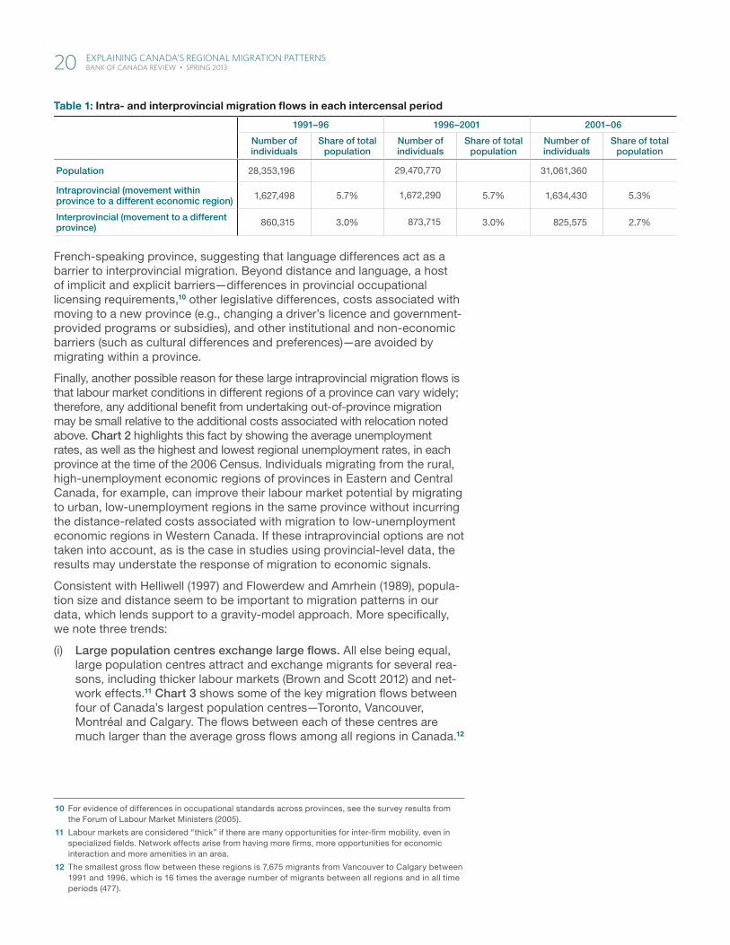
Chart 1 also provides evidence of the importance of intraprovincial migra-tion compared with interprovincial migration. In 2006, population flows within provinces outpaced flows between provinces in 68 of the 73 eco-nomic regions. The relative importance of intraprovincial migration is further confirmed, in aggregate, in Table 1. In all three intercensal periods, intraprovincial migration accounts for approximately two-thirds of the total migration between economic regions in Canada. The data in Table 1 also show that roughly 8.5 per cent of the population, approximately 2.5 million Canadians, moved between regions (either intraprovincial or interprovincial movements) in each of the past three intercensal periods, illustrating that aggregate migration within Canada has been remarkably stable over this period. When disaggregated to the economic region level, however, migra-tion flows and directions can shift dramatically from one census to the next, as the relative economic opportunity between regions changes.8

There are several potential reasons why intraprovincial migration may exceed interprovincial migration. Distances within provinces are, on average, significantly shorter than distances between provinces, and distance is considered to be one of the main barriers to migration.9 Language differ-ences may also play a role. For example, Chart 1 shows that, compared with all other provinces, intraprovincial migration is a much larger source of migrant flows for economic regions in Quebec, which is primarily a

6 Recent migrants are defined as individuals who migrated in the five years since the previous census.

7 Fort McMurray is the economic centre (the largest town or city in the economic region) of the Wood Buffalo-Cold Lake region.

8 For example, the Vancouver Island and Coast region of British Columbia attracted 45,500 net migrants from all other economic regions of Canada’s provinces from 1991 to 1996–a period of strong consumer-led growth in that province. However, from 1996 to 2001, a period in British Columbia dominated by the negative effects of the Asian Crisis, this region received only 2,200 net migrants. Benefiting from the strength of U.S. demand for its exports in the late 1990s, Windsor-Sarnia, Ontario, attracted 2,800 net migrants from 1996 to 2001. In contrast, from 2001 to 2006, this region lost 4,200 net migrants to other economic regions.

9 Indeed, the average distance between two economic regions within the same province is 526 kilometres, whereas the average distance between two regions in different provinces is 2,977 kilometres.

While aggregate migration within Canada is remarkably stable, migration flows between regions can shift dramatically, as relative opportunity changes in response to shocks


Note: Recent migrants are defi ned as individuals who migrated in the fi ve years since the previous census.

Source: Statistics Canada 2006 Census

Wood Buffalo-Cold Lake, ABRed Deer, AB

Banff-Jasper-Rocky Mountain House, ABLaurentides, QC

Thompson-Okanagan, BCNortheast, BC

Athabasca-Grande Prairie-Peace River, ABLanaudière, QC

Vancouver Island and Coast, BCLower Mainland-Southwest, BC

Camrose-Drumheller, ABKootenay, BC

Kitchener-Waterloo-Barrie, ONLethbridge-Medicine Hat, AB

Montérégie, QCSoutheast, MB

Fredericton-Oromocto, NBKingston-Pembroke, ON

Toronto, ONCalgary, AB

Muskoka-Kawarthas, ONEdmonton, AB

Annapolis Valley, NSSouth Central, MB

Estrie, QCStratford-Bruce Peninsula, ON

Moncton-Richibucto, NBSouthwest, MB

Nechako, BCSaskatoon-Biggar, SK

Laval, QCLondon, ON

Outaouais, QCCariboo, BC

Prince Albert, SKInterlake, MBMontréal, QC

Prince Edward IslandCentre-du-Québec, QC

Parklands, MBHamilton-Niagara Peninsula, ON

Ottawa, ONSwift Current-Moose Jaw, SK

Avalon Peninsula, NLYorkton-Melville, SK

North Central, MBBas-Saint-Laurent, QC

Regina-Moose Mountain, SKNorth Shore, NSNorth Coast, BC

Saint John-St. Stephen, NBWest Coast-Northern Peninsula-Labrador, NL

Chaudière-Appalaches, QCNorth, MB

Northeast, ONCapitale-Nationale, QC

Windsor-Sarnia, ONHalifax, NS

Edmundston-Woodstock, NBMauricie, QC

Notre Dame-Central Bonavista Bay, NLAbitibi-Témiscamigue, QC

Winnipeg, MBNorthwest, ON

Northern, SKSouthern, NS

Côte-Nord, QCGaspésie-Îles-de-la-Madeleine, QC

Saquenay-Lac-Saint-Jean, QCCampbellton-Miramichi, NB

Nord-du-Québec, QCSouth Coast-Burin Peninsula, NL

Cape Breton, NS

0

0

5

5

10

10

15

15

20

20

25

25

30

30

35

35

%

%

Intraprovincial Interprovincial External

Chart 1: Share of recent migrants in population, by source, in 2006


French-speaking province, suggesting that language differences act as a barrier to interprovincial migration. Beyond distance and language, a host of implicit and explicit barriers—differences in provincial occupational licensing requirements,10 other legislative differences, costs associated with moving to a new province (e.g., changing a driver’s licence and government-provided programs or subsidies), and other institutional and non-economic barriers (such as cultural differences and preferences)—are avoided by migrating within a province.

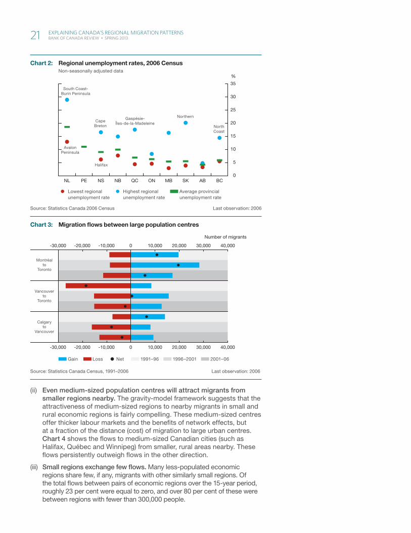
Finally, another possible reason for these large intraprovincial migration flows is that labour market conditions in different regions of a province can vary widely; therefore, any additional benefit from undertaking out-of-province migration may be small relative to the additional costs associated with relocation noted above. Chart 2 highlights this fact by showing the average unemployment rates, as well as the highest and lowest regional unemployment rates, in each province at the time of the 2006 Census. Individuals migrating from the rural, high-unemployment economic regions of provinces in Eastern and Central Canada, for example, can improve their labour market potential by migrating to urban, low-unemployment regions in the same province without incurring the distance-related costs associated with migration to low-unemployment economic regions in Western Canada. If these intraprovincial options are not taken into account, as is the case in studies using provincial-level data, the results may understate the response of migration to economic signals.

Consistent with Helliwell (1997) and Flowerdew and Amrhein (1989), popula-tion size and distance seem to be important to migration patterns in our data, which lends support to a gravity-model approach. More specifically, we note three trends:

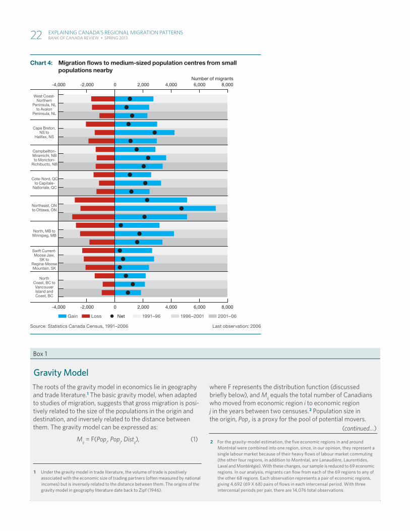
(i) Large population centres exchange large flows. All else being equal, large population centres attract and exchange migrants for several rea-sons, including thicker labour markets (Brown and Scott 2012) and net-work effects.11 Chart 3 shows some of the key migration flows between four of Canada’s largest population centres—Toronto, Vancouver, Montréal and Calgary. The flows between each of these centres are much larger than the average gross flows among all regions in Canada.12

10 For evidence of differences in occupational standards across provinces, see the survey results from the Forum of Labour Market Ministers (2005).

11 Labour markets are considered “thick” if there are many opportunities for inter-firm mobility, even in specialized fields. Network effects arise from having more firms, more opportunities for economic interaction and more amenities in an area.

12 The smallest gross flow between these regions is 7,675 migrants from Vancouver to Calgary between 1991 and 1996, which is 16 times the average number of migrants between all regions and in all time periods (477).

Table 1: Intra- and interprovincial migration fl ows in each intercensal period

1991–96 1996–2001 2001–06

Number of individuals

Share of total population





Population 28,353,196 29,470,770 31,061,360

Intraprovincial (movement within province to a different economic region) 1,627,498 5.7% 1,672,290 5.7% 1,634,430 5.3%

Interprovincial (movement to a different province) 860,315 3.0% 873,715 3.0% 825,575 2.7%


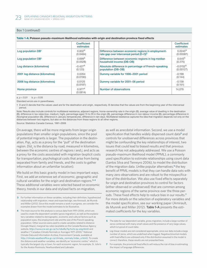
(ii) Even medium-sized population centres will attract migrants from smaller regions nearby. The gravity-model framework suggests that the attractiveness of medium-sized regions to nearby migrants in small and rural economic regions is fairly compelling. These medium-sized centres offer thicker labour markets and the benefits of network effects, but at a fraction of the distance (cost) of migration to large urban centres. Chart 4 shows the flows to medium-sized Canadian cities (such as Halifax, Québec and Winnipeg) from smaller, rural areas nearby. These flows persistently outweigh flows in the other direction.

(iii) Small regions exchange few flows. Many less-populated economic regions share few, if any, migrants with other similarly small regions. Of the total flows between pairs of economic regions over the 15-year period, roughly 23 per cent were equal to zero, and over 80 per cent of these were between regions with fewer than 300,000 people.

Source: Statistics Canada Census, 1991–2006 Last observation: 2006

Gain Loss Net 1991–96 1996–2001 2001–06

-30,000 -20,000 -10,000 0 10,000 20,000 30,000 40,000

Number of migrants

-30,000 -20,000 -10,000 0 10,000 20,000 30,000 40,000

Montréalto

Toronto

Vancouverto

Toronto

Calgaryto

Vancouver

Chart 3: Migration fl ows between large population centres

Units of measure (top of axis):

Verifi ed vs. supplied data, cross-referenced w/ prior artwork

Left alt scale, if applicable

Aligned to outer edgeof axis labels, rag inward towards chart

Chart axes:

Tick marks (major and, if necessary, minor)

“Bookend” tick marks at ends of bottom axis (left/right)

Bottom axis labels placed & verifi ed

Chart bottom region:

Legend items placed and styled

Order verifi ed vs prior artwork

All superscripts, special symbols, etc. as required

Chart footer:

Note(s):

Source(s):

Last observation: (if applicable)

Data presentation styles:

Line styles & stacking order:

Canada/1st

US/2nd

Euro zone/3rd

Japan/4th

UK/5th


US/2nd (proj’d)



UK/5th (proj’d)

All axis lines & ticks

Fill styles & stacking order:

Canada/1st

US/2nd

Euro zone/3rd

Japan/4th UK/5th projected


US/2nd (proj’d)



UK/5th (proj’d)

Control range

Axis lines & ticks

Additional common styles:

dot black

red line plus dot in-chart label

Chart 1: Title+ 2nd line

Sub-title

Source: Statistics Canada 2006 Census Last observation: 2006

Lowest regional unemployment rate

Highest regional unemployment rate

Average provincial unemployment rate

0

5

10

15

20

25

30

35

%

NL PE NS NB QC ON MB SK AB BC

South Coast-Burin Peninsula

AvalonPeninsula

CapeBreton North

Coast

Gaspésie-Îles-de-la-Madeleine

Halifax

Northern

Chart 2: Regional unemployment rates, 2006 CensusNon-seasonally adjusted data


Source: Statistics Canada Census, 1991–2006 Last observation: 2006

Gain Loss Net 1991–96 1996–2001 2001–06

Number of migrants-4,000 -2,000 0 2,000 4,000 6,000 8,000

-4,000 -2,000 0 2,000 4,000 6,000 8,000

West Coast-Northern

Peninsula, NLto Avalon

Peninsula, NL

Cape Breton,NS to

Halifax, NS

Campbellton-Miramichi, NBto Moncton-

Richibucto, NB

Cote-Nord, QCto Capitale-

Nationale, QC

Northeast, ONto Ottawa, ON

North, MB toWinnipeg, MB

Swift Current-Moose Jaw,

SK toRegina-MooseMountain, SK

North Coast, BC to VancouverIsland andCoast, BC

Chart 4: Migration fl ows to medium-sized population centres from small populations nearby

Box 1

Gravity ModelThe roots of the gravity model in economics lie in geography and trade literature.1 The basic gravity model, when adapted to studies of migration, suggests that gross migration is posi-tively related to the size of the populations in the origin and destination, and inversely related to the distance between them. The gravity model can be expressed as:

Mij = F(Popi, Popj, Distij), (1)

1 Under the gravity model in trade literature, the volume of trade is positively associated with the economic size of trading partners (often measured by national incomes) but is inversely related to the distance between them. The origins of the gravity model in geography literature date back to Zipf (1946).

where F represents the distribution function (discussed briefl y below), and Mij equals the total number of Canadians who moved from economic region i to economic region j in the years between two censuses.2 Population size in the origin, Popi, is a proxy for the pool of potential movers.

2 For the gravity-model estimation, the fi ve economic regions in and around Montréal were combined into one region, since, in our opinion, they represent a single labour market because of their heavy fl ows of labour market commuting (the other four regions, in addition to Montréal, are Lanaudière, Laurentides, Laval and Montérégie). With these changes, our sample is reduced to 69 economic regions. In our analysis, migrants can fl ow from each of the 69 regions to any of the other 68 regions. Each observation represents a pair of economic regions, giving 4,692 (69 X 68) pairs of fl ows in each intercensal period. With three intercensal periods per pair, there are 14,076 total observations.

(continued…)


On average, there will be more migrants from larger origin populations than smaller origin populations, since the pool of potential migrants is larger. The population in the destin-ation, Popj, acts as a proxy for the “pull” of the destination region. Distij is the distance by road, measured in kilometres, between the economic centres of regions i and j, and acts as a proxy for the costs associated with migration (explicit costs for transportation, psychological costs that arise from being separated from family and friends, and the costs to gather information about an unfamiliar location).

We build on this basic gravity model in two important ways. First, we add an extensive set of economic, geographic and cultural variables for the origin and destination regions.3, 4 These additional variables were selected based on economic theory, trends in our data and stylized facts on migration,

3 For further information on these variables, including their defi nition, hypothesized relationship with migration, mean and expected sign, see Amirault, de Munnik and Miller (2012). Since this model remains a work in progress, we consider the examples drawn from the model estimates to be illustrative.

4 The main source for this analysis is census data from 1991–2006, which are used to create the dependent variable (gross migration), as well as the explana-tory variables related to demographic, economic and cultural factors such as population sizes, the employment rate and the size of the French-speaking population. Other sources were used to create variables related to distance (googleMaps),marginaltaxrates(availableontheCanadaRevenueagencywebsite, http://www.cra-arc.gc.ca/tx/ndvdls/fq/txrts-py-eng.html) and weather (“Canadian Climate Normals or Averages 1971–2000,” National Climate Data and Information Archive, Environment Canada, available at http://climate.weatheroffice.gc.ca/climate_normals/index_e.html). To create the distance and weather variables, we identify an “economic centre,” which is typically the largest city or town, for each economic region, for example, St. John’s for the Avalon Peninsula, Newfoundland and Labrador.

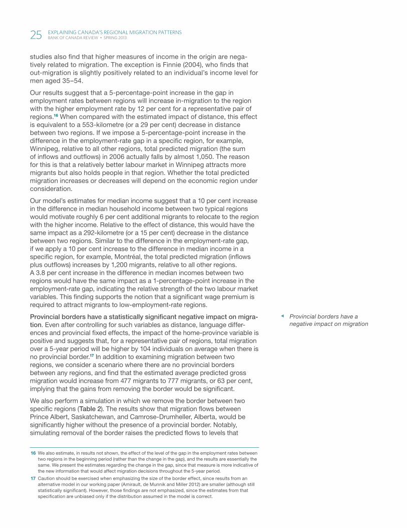
as well as anecdotal information. Second, we use a model specifi cation that handles widely dispersed count data5 and controls for unobserved diff erences across provinces that might be confounding the key relationships of interest, two issues that could lead to biased results and that previous research has not adequately addressed. We use a Poisson pseudo-maximum likelihood model (PPML), a commonly used specifi cation to estimate relationships using count data (Santos Silva and Tenreyro 2006), to model the distribution of the migration data. Unlike popular alternatives,6 the key benefi t of PPML models is that they can handle data sets with many zero observations and are robust to the misspecifi ca-tion of the distribution. We also use fi xed eff ects separately for origin and destination provinces to control for factors (either observed or unobserved) that are common among economic regions of the same province over the three per-iods. These fi xed eff ects help to reduce bias in our results.7 For more details on the selection of explanatory variables and the model specifi cation, see our working paper (Amirault, de Munnik and Miller 2012). Table 1-A presents the esti-mated coeffi cients for the key variables.

5 The data for our dependent variable, gross migration, include a large number of zeros combined with many small values and the presence of very large values, which is typical of count data.

6 Log-linear models are not considered appropriate, since our data include a large number of zeros, which are undefi ned when logged. Negative binomial models with fi xed eff ects are unbiased only if the distribution assumed in the model is correct; therefore, these results are not presented here.

7 For example, the provincial fi xed eff ects will reduce the risk of bias in estimating the impact of language diff erences.

Box 1 (continued)

Table 1-A: Poisson pseudo-maximum likelihood estimates with origin and destination province fi xed effects

Coeffi cient estimates

Coeffi cient estimates

Log population DB† 0.832a (0.0484)

Difference between economic regions in employment-rate gap over intercensal period (D-O)†

0.0245a

(0.00587)

Log population OB† 0.699a (0.0528)

Difference between economic regions in log median household income (DB-OB)

0.645b

(0.275)

Log distance (kilometres) -0.427 a

(0.123)Absolute difference in percentage of French-speaking population (DB-OB)

-0.0152a

(0.00127)

2001 log distance (kilometres) 0.0264 (0.0190)

Dummy variable for 1996–2001 period -0.198 (0.144)

2006 log distance (kilometres) 0.0125 (0.0197)

Dummy variable for 2001–06 period -0.138 (0.151)

Home province 0.977 a

(0.0814)Number of observations 14,076

a. p < 0.01 b. p < 0.05

Standard errors are in parentheses.

† D and O denote that the values used are for the destination and origin, respectively. B denotes that the values are from the beginning year of the intercensal period.

Note: Results also include controls for multilateral resistance, adjacent regions, home-ownership rate in the origin (B), average value of dwelling in the destination (B), difference in tax rates (low, medium, high), percentage aged 15 to 29 in the origin (B), percentage difference in non-labour income (B), percentage difference in Aboriginal population (B), difference in January temperatures, difference in rain days. Multilateral resistance captures the idea that migration depends not only on the distances between two regions, but also on the distances from these regions to all other regions.

Source: Statistics Canada Census, 1991–2006


Influences on Regional MigrationUsing parameter estimates from Box 1, we present findings for popula-tion size and distance that provide support for the use of a gravity-model framework for understanding migration patterns. Furthermore, we discuss the role of labour market variables and barriers to migration (namely, the home-province and language variables) in explaining migration trends over three census periods.

Population sizes in both the origin and the destination have a statistically significant positive effect on the number of migrants that move from one economic region to another. The results from our model suggest that a 10 per cent increase in the destination’s population (approximately 200,000 people) will increase the predicted migration to that region by about 8 per cent for a representative pair of regions over a 5-year period. If we take a given region, for example, Halifax, which had a population of about 356,000 in 2001, a 10 per cent rise in population would increase total pre-dicted migration by about 4,900 people overall (that is, between Halifax and all other 68 economic regions) over a 5-year period.

The distance between economic centres has a negative influence on migration and this effect is statistically significant. For a representative pair of regions, a 10 per cent decrease in the number of kilometres between them would increase the predicted migration by roughly 4 per cent over a 5-year period. From a simulation exercise, our results suggest that if the distances between all regions were halved, the average predicted gross migration would grow by 164, to a total of 641 migrants. To test whether the effect of distance changed over our sample period, we include additional indicator variables for 2001 and 2006 that interact with distance. The posi-tive coefficient estimates for these variables suggest that distance is becoming less restrictive on migration over time; however, the impact on the estimated number of migrants is small and neither variable is statistically significant.13 Note also that the coefficient estimates for the two time indi-cator variables, 2001 and 2006 (1991–96 is the base), in Table 1-A in Box 1, are also statistically insignificant, which implies that average gross migration was not significantly different over time.

Differences in employment rates and in median household incomes have positive and statistically significant effects on migration. In gen-eral, this result is consistent with the previous literature that finds that migration is positively related to the unemployment rate in the origin (Finnie (2004), who investigates individual migration decisions) or the difference in rates between the two regions (Coulombe (2006) and Flowerdew and Amrhein (1989) in aggregate migration studies).14, 15 When considering individual migration decisions (Osberg, Gordon and Lin 1994) or aggregate migration flows (Helliwell 1997; Flowerdew and Amrhein 1989), migration

13 Our working paper (Amirault, de Munnik and Miller 2012) presents an alternative specification that shows statistically significant coefficient estimates for these two interaction variables. While those results provide some evidence that barriers to migration associated with distance have decreased over time, they are not emphasized, since the estimates from that specification are unbiased only if the distribution assumed by the model is correct.

14 Note that this study uses employment rates (the employment to population rate) to measure labour market conditions, while several other studies have used unemployment rates (Coulombe 2006; Finnie 2004; Flowerdew and Amrhein 1989). While both provide information on labour market conditions, weak economic conditions would also lead to lower labour force participation, which the employment rate captures better than the unemployment rate.

15 Some of these studies are not directly comparable with ours, since they examine individual, rather than aggregate, migration (Finnie 2004; Osberg, Gordon and Lin 1994), or focus on net migration (Coulombe 2006).

Population sizes in both the origin and the destination have a positive effect on the number of migrants

The distance between economic centres has a negative influence on migration

Differences in employment rates and in median household incomes have positive effects on migration


studies also find that higher measures of income in the origin are nega-tively related to migration. The exception is Finnie (2004), who finds that out-migration is slightly positively related to an individual’s income level for men aged 35–54.

Our results suggest that a 5-percentage-point increase in the gap in employment rates between regions will increase in-migration to the region with the higher employment rate by 12 per cent for a representative pair of regions.16 When compared with the estimated impact of distance, this effect is equivalent to a 553-kilometre (or a 29 per cent) decrease in distance between two regions. If we impose a 5-percentage-point increase in the difference in the employment-rate gap in a specific region, for example, Winnipeg, relative to all other regions, total predicted migration (the sum of inflows and outflows) in 2006 actually falls by almost 1,050. The reason for this is that a relatively better labour market in Winnipeg attracts more migrants but also holds people in that region. Whether the total predicted migration increases or decreases will depend on the economic region under consideration.

Our model’s estimates for median income suggest that a 10 per cent increase in the difference in median household income between two typical regions would motivate roughly 6 per cent additional migrants to relocate to the region with the higher income. Relative to the effect of distance, this would have the same impact as a 292-kilometre (or a 15 per cent) decrease in the distance between two regions. Similar to the difference in the employment-rate gap, if we apply a 10 per cent increase to the difference in median income in a specific region, for example, Montréal, the total predicted migration (inflows plus outflows) increases by 1,200 migrants, relative to all other regions. A 3.8 per cent increase in the difference in median incomes between two regions would have the same impact as a 1-percentage-point increase in the employment-rate gap, indicating the relative strength of the two labour market variables. This finding supports the notion that a significant wage premium is required to attract migrants to low-employment-rate regions.

Provincial borders have a statistically significant negative impact on migra-tion. Even after controlling for such variables as distance, language differ-ences and provincial fixed effects, the impact of the home-province variable is positive and suggests that, for a representative pair of regions, total migration over a 5-year period will be higher by 104 individuals on average when there is no provincial border.17 In addition to examining migration between two regions, we consider a scenario where there are no provincial borders between any regions, and find that the estimated average predicted gross migration would increase from 477 migrants to 777 migrants, or 63 per cent, implying that the gains from removing the border would be significant.

We also perform a simulation in which we remove the border between two specific regions (Table 2). The results show that migration flows between Prince Albert, Saskatchewan, and Camrose-Drumheller, Alberta, would be significantly higher without the presence of a provincial border. Notably, simulating removal of the border raises the predicted flows to levels that

16 We also estimate, in results not shown, the effect of the level of the gap in the employment rates between two regions in the beginning period (rather than the change in the gap), and the results are essentially the same. We present the estimates regarding the change in the gap, since that measure is more indicative of the new information that would affect migration decisions throughout the 5-year period.

17 Caution should be exercised when emphasizing the size of the border effect, since results from an alternative model in our working paper (Amirault, de Munnik and Miller 2012) are smaller (although still statistically significant). However, those findings are not emphasized, since the estimates from that specification are unbiased only if the distribution assumed in the model is correct.

Provincial borders have a negative impact on migration


are much closer to those between Prince Albert and Saskatoon-Biggar, Saskatchewan—a destination similar to Camrose-Drumheller, Alberta, in terms of distance and labour market conditions, but within the same province.18

Language differences reduce migration between regions. This result is consistent with findings in Helliwell (1997) and Flowerdew and Amrhein (1989). Helliwell (1997) uses an indicator variable for flows to and from Quebec as a control for language differences, which improves the overall fit of the model. Finnie (2004) also finds that language differences are important for individual migration decisions. In our estimation, which includes provincial fixed effects in the origin and destination, a 10-percentage-point difference between two regions’ share of their populations that is French-speaking decreases the predicted number of migrants by 15 per cent. To put this into perspective, a 2.3 per cent increase in median income, or a 0.6-percentage-point increase in the employment-rate gap, is needed to offset the disincentive to migrate cre-ated by a 1-percentage-point increase in the difference in the share of the population that is French-speaking between two regions. Given that the average difference in the share of the population that is French-speaking between two economic regions is 30.8 percentage points, the total effect could be much greater in some regions.

Other variables of interest from an economic perspective are relative income tax rates and housing market variables. Our research finds that higher marginal tax rates at lower income levels increase migration inflows, while higher rates for the highest-income earners reduce them. We interpret this result to mean that higher tax rates for lower-income earners signal better services. For higher-income earners, higher taxes represent a greater rela-tive burden. Home-ownership rates in the region of origin have a meaningful negative effect on migration, while housing prices in the destination have no significant effect. For more details on these and other results, see Amirault, de Munnik and Miller (2012).

ConclusionUsing data for sub-provincial economic regions (each representing a grouping of census subdivisions), we find that differences in both employ-ment rates and household incomes are positively related to migration flows and help to explain Canadian migration patterns. Such results provide evidence that migrants respond to economic signals and that they are a key element in the stabilization process following economic shocks. Our estimates also suggest that, even after controlling for origin and destination provincial fixed effects, language differences restrict migration.

18 Note, however, that the actual flows of migrants from Prince Albert to Saskatoon-Biggar, Saskatchewan, in these three periods are much higher than the model predicts.

Language differences reduce migration between regions

Table 2: Simulations of migration fl ows with and without a provincial border

Predicted gross migration

Flow Intercensal period With border Without border

Prince Albert, Saskatchewan, to Camrose-Drumheller, Alberta

1991–961996–20012001–06

744889687

1,9472,3611,825

Prince Albert to Saskatoon-Biggar, Saskatchewan

1991–961996–20012001–06

---

3,3982,9242,824


We also find that provincial borders are negatively related to migration flows. This implies that obstacles to interprovincial mobility remain. While the Agreement on Internal Trade came into effect in 1995 with the objective of removing barriers to mobility across provinces,19 no empirical evidence has quantified the impact of this initiative. The situation requires an increase in awareness of these issues and a sustained effort at improvement (Gomez and Gunderson 2007; Grady and Macmillan 2007). It would be interesting to investigate whether the border effect reflects occupational licensing differ-ences, the lower costs of remaining in the same province or simply prefer-ences. If barriers created by provincial borders can be removed, easier labour mobility would ultimately facilitate macroeconomic adjustment and possibly result in stronger productivity growth (Leung and Cao 2009).

19 Specifically, these barriers were in the areas of (i) residency requirements; (ii) licensing, certification and registration of workers; and (iii) recognition of occupational qualifications (Gomez and Gunderson 2007; Grady and Macmillan 2007).

Literature CitedAmirault, D., D. de Munnik and S. Miller. 2012. “What Drags and Drives

Mobility: Explaining Canada’s Aggregate Migration Patterns.” Bank of Canada Working Paper No. 2012-28.

Audas, R. and J. T. McDonald. 2003. “Employment Insurance and Geographic Mobility: Evidence from the SLID.” Social Research and Demonstration Corporation Working Paper No. 03-03.

Brown, M. W. and D. M. Scott. 2012. “Cities and Growth: Human Capital Location Choice: Accounting for Amenities and Thick Labour Markets.” Statistics Canada Cat. No. 11-622-M — No. 027.

Coulombe, S. 2006. “Internal Migration, Asymmetric Shocks, and Interprovincial Economic Adjustments in Canada.” International Regional Science Review 29 (2): 199–223.

Finnie, R. 2004. “Who Moves? A Logit Model Analysis of Inter-Provincial Migration in Canada.” Applied Economics 36 (16): 1759–79.

Flowerdew, R. and C. Amrhein. 1989. “Poisson Regression Models of Canadian Census Division Migration Flows.” Papers in Regional Science 67 (1): 89–102.

Forum of Labour Market Ministers. 2005. Report of Survey Results: Inter-Provincial Labour Mobility in Canada 2004/05, 18 May.

Gomez, R. and M. Gunderson. 2007. “Barriers to the Inter-Provincial Mobility of Labour.” Industry Canada Working Paper No. 2007-09.

Grady, P. and K. Macmillan. 2007. “Inter-Provincial Barriers to Labour Mobility in Canada: Policy, Knowledge Gaps and Research Issues.” Industry Canada Working Paper No. 2007-10.


http://ideas.repec.org/p/pra/mprapa/2988.html

http://ideas.repec.org/p/pra/mprapa/2988.html

Greenwood, M. J. 1997. “Internal Migration in Developed Countries.” Chapter 12 in Handbook of Population and Family Economics, edited by M. R. Rosenzweig and O. Stark, 647–720. New York: Elsevier Science B.V.

Helliwell, J. F. 1997. “National Borders, Trade and Migration.” Pacific Economic Review 2 (3): 165–85.

Lefebvre, M. and S. S. Poloz. 1996. “The Commodity-Price Cycle and Regional Economic Performance in Canada.” Bank of Canada Working Paper No. 96-12.

Leung, D. and S. Cao. 2009. “The Changing Pace of Labour Reallocation in Canada: Causes and Consequences.” Bank of Canada Review (Summer): 31–41.

Macklem, T. 2012. “A Measure of Work.” Speech to the Winnipeg Chamber of Commerce, Winnipeg, Manitoba, 4 October.

McCallum, J. 1995. “National Borders Matter: Canada-U.S. Regional Trade Patterns.” American Economic Review 85 (3): 615–23.

Osberg, L., D. Gordon and Z. Lin. 1994. “Interregional Migration and Interindustry Labour Mobility in Canada: A Simultaneous Approach.” Canadian Journal of Economics 27 (1): 58–80.

Santos Silva, J. M. C. and S. Tenreyro. 2006. “The Log of Gravity.” Review of Economics and Statistics 88 (4): 641–58.

Stillwell, J. 2005. “Inter‐Regional Migration Modelling: A Review and Assessment.” In Land Use and Water Management in a Sustainable Network Society, 1–26. Proceedings of the 45th Congress of the European Regional Science Association, held by Vrije Universiteit Amsterdam, 23–27 August. Amsterdam: Vrije Universiteit Amsterdam.

Zimmermann, K. F. and T. K. Bauer. 2002. The Economics of Migration. Cheltenham, UK: Edward Elgar Publishing.

Zipf, G. K. 1946. “The P1P2/D Hypothesis: On the Intercity Movement of Persons.” American Sociological Review 11 (6): 677–86.


Modelling the asset-allocation and liability strategy for Canada’s foreign Exchange reservesFrancisco Rivadeneyra, Jianjian Jin, Narayan Bulusu and Lukasz Pomorski, Funds Management and Banking Department

� Canada’s official international reserves are held with the objective of aiding in the control and protection of the external value of the Canadian dollar, and are managed to provide foreign currency liquidity to the federal government.

� Unlike in many other countries, Canada’s foreign exchange reserves are owned by the federal government and managed jointly by the government and the Bank of Canada.

� Canada’s use of an asset-liability-matching (ALM) framework limits exposure to interest rate and exchange rate risks.

� To enhance the policy advice that supports the management of the foreign exchange reserves portfolio, the Bank has developed an ALM portfolio model that quantifies the trade-offs between risk, return, liqui-dity and funding costs in asset and liability decisions.

The 2007–09 global financial crisis led to rapid accumulation of foreign reserves in both developed and emerging countries and triggered discus-sions of how these reserves should be managed.1 While efforts to reassess and improve the management of Canada’s reserves date back to before the crisis, recent events have highlighted the need for appropriate tools to aid policy-makers in their management of the reserves.

Canada’s foreign exchange reserves help to promote orderly conditions for the Canadian dollar in foreign exchange markets, if required, and provide foreign currency liquidity to the federal government. These reserves are not included on the balance sheet of the central bank; instead, they belong to the federal government and are held primarily in the Exchange Fund Account (EFA). Unlike many other countries, the assets held in the EFA are funded by Government of Canada liabilities denominated in, or converted to, foreign currencies. The Bank of Canada acts as the fiscal agent for the government in the management of the EFA and works with the Department of Finance to advise the Minister of Finance on the funding and investment of Canada’s foreign exchange reserves.

1 For a detailed discussion, see IMF (2011).


29 ModElling ThE assET-alloCaTion and liabiliTy sTraTEgy for Canada’s forEign ExChangE rEsErvEs BankofCanadaReview•SpRing2013

This article describes an analytical tool recently developed at the Bank, which, combined with other information, guides policy advice on the management of Canada’s foreign exchange reserves and the liabilities used to finance them. We begin by discussing the objectives of the EFA, its governance framework and its investment principles. We then examine the portfolio-management model developed to help policy-makers achieve the EFA’s objectives in an efficient and fiscally responsible manner. Finally, we present some of the insights gained from this tool.

The Exchange Fund AccountThe objective of the EFA, as stipulated in the Currency Act, is to assist in the control and protection of the external value of the Canadian dollar. The Currency Act confers upon the Minister of Finance the authority to acquire, borrow, sell or lend assets held in the EFA in accordance with the Statement of Investment Policy (SIP) for the Government of Canada.2 The SIP specifies operational measures to achieve the EFA’s objective, elucidates principles of investment that govern its management and specifies risk-exposure limits based on prudential asset-management practices.

The SIP requires that EFA assets be invested in a combination of liquid and safe short-term instruments and high-quality medium- and long-term instru-ments that help to achieve the highest possible level of return without jeopard-izing liquidity and capital-preservation objectives. The SIP also requires the EFA to be managed in a cost-effective, transparent and accountable manner, following leading risk-management practices, and outlines an oversight and governance structure to ensure adherence to investment principles.

EFA assets comprise primarily liquid foreign currency securities (largely government treasury bills and bonds); deposits with commercial banks, central banks and the Bank for International Settlements; special drawing rights (SDRs);3 and a small holding of gold.4 The SIP specifies that the Government of Canada liabilities that fund the liquid securities be matched as closely as possible in currency and duration to the interest and principal receipts and payments on EFA assets in order to minimize the government’s exposure to currency and interest rate risks.5 These matching require-ments—referred to as the asset-liability-matching (ALM) framework—are relatively unique among managers of sovereign reserves.

The size of the EFA has increased steadily since 1998. As of February 2013, it had over US$65 billion in assets, and, as shown in Chart 1, securities holdings were its most important component.6 The spike in assets in 2009 was the result of the allocation of SDRs to Canada as part of the International Monetary Fund’s program to supplement the SDR positions of member countries. As of February 2013, U.S.-dollar assets accounted

2 The latest SIP is in Annex 1 of the Report on the Management of Canada’s Official International Reserves at http://www.fin.gc.ca/activty/oirrep/oir-roli-12-eng.asp#toca1.

3 An SDR is an international reserve asset created by the International Monetary Fund (IMF). Its value is defined by a weighted basket of the U.S. dollar, the euro, the British pound and the Japanese yen.

4 Canada’s official international reserves, the majority of which are in the EFA, also include Canada’s reserve position at the IMF. This position, which represents Canada’s investment in the activities of the IMF, fluctuates according to IMF drawdowns and repayments.

5 “Duration matching,” also known as “duration immunization,” is a strategy in which the durations of assets and liabilities are matched so that changes in interest rates have similar offsetting effects on the values of both assets and liabilities, thereby making a portfolio insensitive to small changes in interest rates.

6 These assets were funded by dedicated foreign currency borrowings with a par value of US$51 billion as of 31 March 2012.

Liabilities that fund the Exchange Fund Account are matched as closely as possible in currency and duration to the interest and principal receipts and payments on EFA assets


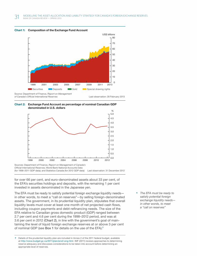
for over 66 per cent, and euro-denominated assets about 33 per cent, of the EFA’s securities holdings and deposits, with the remaining 1 per cent invested in assets denominated in the Japanese yen.

The EFA must be ready to satisfy potential foreign exchange liquidity needs—in other words, to meet a “call on reserves”—by selling foreign-denominated assets. The government, in its prudential liquidity plan, stipulates that overall liquidity levels must cover at least one month of net projected cash flows, including coupon payments and debt-refinancing needs. The size of the EFA relative to Canadian gross domestic product (GDP) ranged between 2.7 per cent and 4.6 per cent during the 1998–2012 period, and was at 3.6 per cent in 2012 (Chart 2), in line with the government’s goal of main-taining the level of liquid foreign exchange reserves at or above 3 per cent of nominal GDP (see Box 1 for details on the use of the EFA).7

7 Details of the prudential liquidity plan are included in Annex 2 of the 2011 federal budget, available at http://www.budget.gc.ca/2011/plan/anx2-eng.html. IMF (2011) reviews approaches to determining reserve adequacy and discusses considerations to be taken into account before determining an appropriate level of reserves.

The EFA must be ready to satisfy potential foreign exchange liquidity needs—in other words, to meet a “call on reserves”

Source: Department of Finance, Report on Management of Canada’s Offi cial International Reserves Last observation: 28 February 2013

Securities Deposits Gold Special drawing rights

1999 2001 2003 2005 2007 2009 2011 20130

10

20

30

40

50

60

70

80US$ billions

Chart 1: Composition of the Exchange Fund Account

Sources: Department of Finance, Report on Management of Canada’s Offi cial International Reserves; World Bank National Accounts Data (for 1998–2011 GDP data); and Statistics Canada (for 2012 GDP data) Last observation: 31 December 2012

1998 2000 2002 2004 2006 2008 2010 2012

%

0.0

0.5

1.0

1.5

2.0

2.5

3.0

3.5

4.0

4.5

5.0

Chart 2: Exchange Fund Account as percentage of nominal Canadian GDP denominated in U.S. dollars


http://www.budget.gc.ca/2011/plan/anx2-eng.html

The Minister of Finance governs the EFA, approves key initiatives such as strategic plans and investment policies, and provides an annual report on the operations of the EFA to Parliament.8 The design of key strategies and policies, the oversight of operations, and the coordination of funding, investment and liquidity-management activities are delegated to the EFA’s Funds Management Committee, to which the Risk Committee and the Asset Liability Management Committee provide advice. Officials from the Bank of Canada and the Department of Finance form all three committees. Policy-analysis tools developed by the Bank, of which the ALM portfolio model is one, are intended to help organize the discussion among policy-makers, who could use them in conjunction with their judgment and risk preferences. The EFA’s day-to-day investment and funding transactions are executed by the Bank of Canada.9

The Modelling ApproachThe Bank recently developed the ALM portfolio model to enhance the quality of the policy advice provided to the committees managing the for-eign exchange reserves. The model determines the combinations of assets and liabilities with the same duration and currency that maximize the returns (net of funding costs) for each possible level of portfolio risk, while also satisfying the preference for liquid assets.

A target portfolio could then be determined using output from the model, risk preferences and professional judgment, including considerations of overall risk measures (such as value at risk, among others).10 This

8 The electronic versions of these reports for recent years are archived at http://www.fin.gc.ca/purl/efa-eng.asp.

9 The Funds Management Governance Framework (available at http://www.fin.gc.ca/treas/Goveev/pdf/FMGF_e.pdf) describes the roles and responsibilities of officials at the Department of Finance and the Bank of Canada, and of the committees established to govern funds-management activities.

10 A review of the asset-allocation framework conducted in 2012 recommended incorporating enhanced portfolio-management methods into the EFA’s decision-making process. The incorporation and use of quantitative tools in the investment-management process are in response to the recommendations of that review. Details of the report are available at http://www.fin.gc.ca/treas/evaluations/eaafefa-ecracfc-eng.asp.

The ALM portfolio model determines the combinations of assets and liabilities with the same duration and currency that maximize the returns for each possible level of portfolio risk

Box 1

Evolution of the Government’s Policy Toward Intervention in the Foreign Exchange MarketCanada’s policy toward intervening in the foreign exchange market has evolved over the past 15 years. Until September 1998, to maintain orderly conditions for the Canadian dollar in the foreign exchange market, intervention was generally predictable and automatic—selling foreign currency and buying Canadian dollars when there was downward pressure on the exchange rate, and vice versa when there was upward pressure on the value of the Canadian dollar. As Canada’s foreign exchange market matured and became increasingly liquid, policy-makers decided that such an intervention policy was no longer required. Since September 1998, the policy of the Department of Finance and the Bank of Canada has been to consider intervening if there are signs of a serious near-term market breakdown indicating a severe lack of liquidity in the market for the Canadian dollar, or if extreme currency movements seriously threaten the conditions that support sustainable long-term growth of the Canadian economy. In addition, the current intervention policy allows for Canada’s

participation in coordinated interventions with other central banks to infl uence the value of a foreign currency. As of early 2013, there have been only two interventions since 1999, and both were coordinated actions with other central banks. The fi rst was to support the euro by purchasing US$97 million worth of that currency in September 2000, and the second was to stabilize the Japanese currency market by selling yen equalling US$124 million in value in March 2011, as agreed by theg-7ministersoffinance.1

1 Details of offi cial interventions are included in the annual Report on the Management of Canada’s Offi cial International Reserves. The Financial Review section of the Exchange Fund Account Annual Report for 1999 (available at http://www.fin.gc.ca/efa-cfc/efa1999_1-eng.asp) and the Bank of Canada backgrounder Intervention in the Foreign Exchange Market (avail-able at http://www.b ankofcanada.ca/wp-content/uploads/2010/11/intervention_foreign_exchange.pdf) discuss the rationale for the change in Canada’s intervention practices implemented in September 1998. Management reports beginning in 2000 refl ect the modifi ed criteria under which an interven-tion in the foreign exchange market might be considered.


http://www.fin.gc.ca/purl/efa-eng.asp

http://www.fin.gc.ca/purl/efa-eng.asp

http://www.fin.gc.ca/treas/Goveev/pdf/FMGF_e.pdf

http://www.fin.gc.ca/treas/Goveev/pdf/FMGF_e.pdf

http://www.fin.gc.ca/treas/evaluations/eaafefa-ecracfc-eng.asp

http://www.bankofcanada.ca/wp-content/uploads/2010/11/intervention_foreign_exchange.pdf

http://www.bankofcanada.ca/wp-content/uploads/2010/11/intervention_foreign_exchange.pdf

multi-stage decision-making process can help reduce modelling risks, while also benefiting from policy-makers’ knowledge of financial markets. The model also helps to evaluate the costs of the matching requirements for currency and duration, as well as other guidelines set out in the SIP.

Two particular characteristics of the EFA determine the modelling approach. The first is that its main objective is to provide foreign currency liquidity to the government, if and when required. The preference for liquid assets is therefore a key component of the model. The second is that, in contrast to the management of most liability-driven funds in which the level of liabilities is fixed, policy-makers can choose the size and composition of both assets and liabilities, as long as the interest rate and exchange rate risks are man-aged according to the ALM framework.

To clarify the ALM model, we first provide separate explanations of the trade-offs involved in the asset-allocation and funding-mix decisions. The EFA’s asset-allocation decision involves risk-return and liquidity trade-offs; the funding-mix decision includes liability cost and risk trade-offs. We then show how the ALM model allows policy-makers to evaluate both sets of trade-offs simultaneously.

Optimizing the asset allocationTo find a mix of assets that balances the policy-makers’ preferences, the ALM model augments the traditional mean-variance analysis (Markowitz 1952) with a preference for liquidity. Mean-variance analysis captures the risk-return trade-off between assets (riskier assets usually promise higher expected returns), while emphasizing diversification, which lowers the port-folio’s risk by avoiding excessive concentration in any one asset.

The model finds the best combinations of assets by balancing the prefer-ences for liquidity and returns. Generally, highly liquid assets have lower transaction costs, but also lower returns. These assets remain liquid during times of financial distress, and their transaction costs vary less between good and bad economic conditions (Rivadeneyra 2012).

Another critical dimension of the asset-allocation problem is maintaining the liquidity of the portfolio after a call on reserves (Romanyuk 2010). The model balances the transaction costs associated with meeting a call on reserves with the need to ensure that the remaining assets are sufficiently liquid to meet potential calls on reserves in the future at a reasonable cost. If a man-ager minimized the immediate cost of a call on reserves by selling the assets with the lowest transaction costs (for example, U.S. Treasury securities), this would leave a higher concentration of assets that are less liquid in the EFA. Any subsequent calls on reserves would require selling large amounts of these assets, which would be disproportionately more expensive than spreading the sales over several episodes. Taking the costs of meeting future calls on reserves into consideration, the model recommends that the initial call on reserves be met with a diversified selection of assets, thus preserving the liquidity of the remaining portfolio, and that the initial choice of assets held in the EFA be tilted toward highly liquid assets.

The outputs of the model are, for each level of risk, the optimal asset weights and a liquidation strategy that satisfies a call on reserves. An addi-tional benefit of this approach is that it quantifies the cost of maintaining a highly liquid portfolio by comparing the expected returns of the model with those of a traditional allocation based on mean-variance analysis.


Optimizing the funding mixReserve assets are funded mainly by converting Canadian-dollar liabilities issued by the government into foreign currency liabilities through cross-currency swaps and by direct issuance of foreign currency securities. Cross-currency swaps are derivatives contracts with private financial institu-tions through which the Bank of Canada, on behalf of the Government of Canada, exchanges the principal and future interest payments of a liability denominated in Canadian dollars for a liability denominated in one of the EFA currencies.11

Finding the optimal mix of funding for the EFA is similar to other public debt-management practices that attempt to balance objectives to minimize cost and risk (Missale 2000). Canada typically obtains more cost-effective foreign currency funding using cross-currency swaps; however, these transactions carry counterparty risk, which could induce volatility in the government’s budgetary position (Rivadeneyra and Dissou 2011).12 The importance of counterparty risk is reinforced by the observation that counterparty credit losses could materialize during episodes in which a call on reserves may occur. The model incorporates this risk through a credit charge for issuing cross-currency swaps that increases with exposure to a particular counter-party. Likewise, the model incorporates rollover risk, which arises from con-centrating the funding in a particular part of the term structure, by including charges on funding plans that concentrate issuance in a narrow range of maturities. These charges are calibrated using judgment and past experience.

The model output is the optimal mix across different instruments and matur-ities that minimizes the funding cost (interest paid on the liabilities), subject to restrictions placed on risk measures. One of the main insights from the model is that most of the mark-to-market volatility in the asset-liability gap comes from the total share of cross-currency swaps in the funding of the EFA. A second insight is that the composition of the asset portfolio has a significant impact on the optimal funding mix, since it constrains the liabil-ities to a specific duration. This highlights the need to consider the asset and liability decisions together, and reinforces the importance of the ALM framework under which Canada’s foreign exchange reserves are managed.

Combining decisions on asset allocation and funding mixThe ALM model combines the analyses of the individual decisions regarding the optimal asset allocation and funding mix subject to the constraint to match the duration and currency of assets and liabilities. Its output is the efficient frontier, or the potential combinations of EFA assets that provide the maximum level of return for a given level of risk and the corresponding liabilities used to fund these assets.

The model demonstrates that the ALM framework requirement to match currency and duration restricts the range of potential portfolios and reduces net expected returns (Figure 1). The reduction in choice is seen in the short-ened span of the efficient frontier when ALM is imposed, and the reduction in expected net portfolio returns is represented by the vertical distance between the curves for a given level of risk.

11 See De León (2000–2001) for a complete list of the funding sources. The “Debt Management Report” for the 2011–12 fiscal year, available at http://www.fin.gc.ca/dtman/2011-2012/dmr-rgd1201-eng.asp, provides additional details on the funding sources.

12 Counterparty risk can induce budgetary volatility if a counterparty does not fulfill its obligations when the mark-to-market value of the cross-currency swaps favours the government. Mark-to-market value is a measure of the fair value of an asset based on its current market price, or the market price of a similar asset.

The composition of the asset portfolio has a significant impact on the optimal funding mix, since it constrains the liabilities to a specific duration

The ALM framework requirement to match currency and duration restricts the range of potential portfolios and reduces net expected returns


http://www.fin.gc.ca/dtman/2011-2012/dmr-rgd1201-eng.asp

The model shows that the main reason for the reduction in expected net returns under the ALM framework is an increase in funding costs, instead of a decrease in asset returns. This is because when ALM is imposed, minimizing funding costs is subject to the constraint that the asset portfolio and the mix of liabilities have the same duration. The liability mix cannot attain the lowest total cost—achieved by balancing more expensive long-term liabilities with less expensive short-term liabilities that have higher rollover risks—since the lowest-cost mix will not have the same duration as that of the optimal asset portfolio for all levels of risk. The lower net returns under the ALM framework shown in Figure 1 are the result of most asset portfolios along the frontier being funded with a more expensive liability mix.13 The liability structure under the ALM model limits the range of possible duration and, in turn, the range of the portfolio’s risk, thus restricting the span of the optimal frontier.

An additional feature of the ALM model is that it helps to quantify the costs of managing risks that arise in the presence of an asset-liability gap in the foreign currency reserves, i.e., when the value of assets is different from that of the liabilities. This gap may result either from temporary differentials in the mark-to-market value of assets and liabilities, or from a call on reserves that requires selling assets, thus making their value fall below that of the liabil-ities. Depending on movements in exchange rates or interest rates, an asset-liability gap exposes the government to risk, since it would need to budget additional public funds to cover the gap. The model quantifies the trade-offs involved in maintaining the ALM framework under these condi-tions. It shows that duration immunization creates a tension between holding longer-duration assets and holding assets with high liquidity and returns, especially after a call on reserves.

By providing a rigorous framework to conduct scenario analysis, the ALM model also allows for an examination of how the optimal asset and funding outcomes vary in response to changes in economic conditions.

13 The two efficient frontiers in Figure 1 coincide at the point where the optimal assets have the same duration as that of the lowest-cost mix of liabilities.

The ALM model also helps to quantify the costs of managing risks that arise in the presence of an asset-liability gap in the foreign currency reserves

Source: Bank of Canada

Effi cient frontier (without asset-liability matching)

Effi cient frontier (with asset-liability matching)

Net portfolioreturns

Portfolio risk

Figure 1: The effi cient frontier and the costs of asset-liability matching


By quantifying the trade-offs involved in managing the EFA and providing analyses that supplement experienced economic judgment, the model could help policy-makers to make better decisions.

ConclusionGreater uncertainty in global financial markets and the accompanying increase in sovereign risks have led to a reassessment of the framework for the EFA asset-allocation and funding-mix decision. The ALM portfolio model developed by the Bank of Canada is part of a renewed decision-making process that places Canada at the forefront of countries using the ALM approach to manage their foreign exchange reserves.

The ALM model helps to evaluate the attractiveness of some asset classes for the EFA by quantifying their contribution to the returns and risks of the portfolio. The model can also quantify changes in the relative costs of dif-ferent funding sources, allowing policy-makers to effectively manage the recent increase in counterparty risks.

The Bank of Canada is engaged in a process of continuous improvement of its policy advice. New portfolio-management models—incorporating methods generated by academic research, along with lessons learned from the use of the ALM model—are being developed to better meet the objective of the EFA, while reducing operating costs and improving its governance.

Literature CitedDe León, J. 2000–2001. “The Bank of Canada’s Management of Foreign

Currency Reserves.” Bank of Canada Review (Winter): 13–21.

International Monetary Fund (IMF). 2011. “Assessing Reserve Adequacy.” Available at http://www.imf.org/external/np/pp/eng/2011/021411b.pdf.

Markowitz, H. 1952. “Portfolio Selection.” Journal of Finance 7 (1): 77–91.

Missale, A. 2000. Public Debt Management. Oxford: Oxford University Press.

Rivadeneyra, F. 2012. “The U.S.-Dollar Supranational Zero-Coupon Curve.” Bank of Canada Discussion Paper No. 2012-5.

Rivadeneyra, F. and O. Dissou. 2011. “A Model of the EFA Liabilities.” Bank of Canada Discussion Paper No. 2011-11.

Romanyuk, Y. 2010. “Liquidity, Risk, and Return: Specifying an Objective Function for the Management of Foreign Reserves.” Bank of Canada Discussion Paper No. 2010-13.


http://www.imf.org/external/np/pp/eng/2011/021411b.pdf

Documents

Bank of Canada Review · The Bank of Canada Review is published four times a year. Articles undergo a thorough review process. The views expressed in the articles are those of the