Bank Diversification, Market

Structure and Bank Risk Taking:

Evidence from U.S. Commercial Banks

Martin Goetz∗

April 18, 2012

Abstract

This paper studies how a bank’s diversification affects its own risk taking

behavior and the risk taking of competing, nondiversified banks. In particular,

I test whether greater geographic diversification of banks has effects on the

risk taking behavior of nondiversified competitors beyond effects on risk due

to competition. Empirical results obtained from the U.S. commercial banking

sector indicate that a bank’s risk taking is lower when its competitors have

a more diversified branch network. By utilizing the state-specific timing of a

removal of intrastate branching restrictions in two identification strategies, I

further pin down a causal relationship between the diversification of competi-

tors and a bank’s risk taking behavior. These findings indicate that a bank’s

diversification also impacts the risk taking of competitors, even if these banks

are not diversifying their activities.

JEL Classification: G21, G32, L22

Keywords: Risk Taking, Competition, Commercial Banks, Diversification

∗Federal Reserve Bank of Boston, 600 Atlantic Avenue, Boston MA 02210. Email: Mar-tin.Goetz@bos.frb.org. Tel.: (617) 973 3018Financial support from the Networks Financial Institute (Indiana State University) is greatly ap-preciated. I am very thankful to Ross Levine, Nicola Cetorelli, Marcia Millon Cornett, RubenDurante, Tatiana Farina, Andy Foster, Juan Carlos Gozzi, Luc Laeven, Alex Levkov, Jose Liberti,Blaise Melly, Donald Morgan, and David Van Hoose for helpful comments and discussions. I alsothank seminar participants at the Bank for International Settlements, Banque de France, Bent-ley College, Board of Governors, Brown University, European Business School, European CentralBank, Federal Reserve Bank of Boston, FGV-EESP and Tilburg University for many commentsand suggestions. The views expressed in this paper are solely those of the author and do notnecessarily reflect official positions of the Federal Reserve Bank of Boston or the Federal ReserveSystem.

1 Introduction

In this paper, I address one of the most basic questions in banking: are banks

with lending activities in several banking markets safer than banks that focus their

operations on a single market? Expanding lending operations into more markets

allows banks to diversify risk across regions, and if loan returns across regions are

not perfectly correlated, geographically diversified banks are safer because they are

less exposed to shocks that hit individual areas (Diamond (1984); Demsetz and

Strahan (1997); Morgan et al. (2004)).

The diversification of banks might also change their behavior in the market

for borrowers, which in turn affects competition and banks’ risk taking. This might

occur in addition to the aforementioned bank-specific effects of geographic expansion

as a bank’s risk taking behavior is also affected by market competition. On the one

hand, the expansion of banks might intensify competition, which decreases a bank’s

rents, erodes its charter value, and provides incentives for banks to take on more

risk (Keeley (1990), Allen and Gale (2000)). Greater competition, on the other

hand, might also lead to lower loan rates, which reduces the extent of borrowers’

risk shifting incentives and thus decreases a bank’s exposure to risk of failure (Boyd

and de Nicolo (2005), Boyd et al. (2009a)). Moreover, the diversification of a bank

changes its organizational structure, which might affect its lending decisions and

has ramifications for competing banks, even if competitors are not diversifying their

operations geographically (Stein (2002), Berger et al. (2005)). Hence, the expansion

of banks can have effects on their risk taking and the risk taking of competitors, but

these effects can be quite different for diversifying and nondiversifying banks.

I provide empirical evidence from the U.S. banking sector indicating that in-

teractions between banks that diversify geographically and those that focus their

operations are important when examining bank risk taking since I find that the

diversification of banks has direct effects on the risk taking behavior of local, non-

1

diversifying competitors beyond effects of market competition on bank risk. While

many researchers examine the connection between changes in competition or diver-

sification and risk taking across markets, none consider how interactions between

banks that diversify and banks that focus their operations affect the fragility of these

different banks. Non-expanding commercial banks, however, are an important part

of the U.S. banking sector as they constitute the majority of chartered commer-

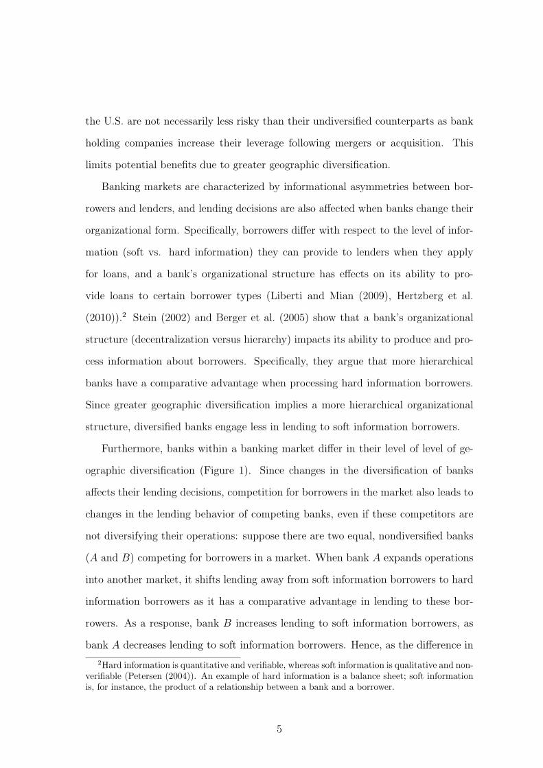
cial banks in the U.S. Figure 1(a) shows that in 1976, nine out of ten commercial

banks only operated branches in one single county. Thirty years later (Figure 1(b)),

still more than half of all commercial banks in the U.S. had branches in one single

county.1

Using information from the U.S. commercial banking sector, I empirically exam-

ine the relationship between a bank’s geographical diversification, the diversity of

its competitors and the risk taking behavior of these different banks. By examining

banks’ level of geographic diversification across counties within a state, I find that

a bank’s risk taking is lower when its competitors have a more diversified branch

network across counties. This effect is robust to the inclusion of variables that cap-

ture the degree of competition within a banking market (Boyd et al. (2007)) and

the difference between a bank’s diversification and the diversification of competitors

is significantly associated with risk taking beyond effects through banking market

competition. This finding is also not sensitive to the definition of risk taking and

diversification. These results, however, do not reflect a causal relationship since

unobservable factors, such as bank efficiency, might exert an influence on a bank’s

risk taking behavior.

I employ two empirical strategies based on (1) the timing of intrastate branch-

ing deregulation and (2) the relationship between intrastate branching deregulation,

distance and bank characteristics to explain a bank’s expansion behavior within a

1Banks with branches are small, but are sizeable on an aggregate level: in 2006, banks withbranches in only one county held approximately 11% of total deposits.

2

state to estimate the causal impact of a bank’s diversification on competing banks’

risk taking. Because banks were not allowed to expand their branch network freely

within state borders before the removal of these branching restrictions, I can identify

the exogenous component of banks’ expansion activity, as each identification strat-

egy utilizes the state specific timing of a removal of intrastate branching restrictions

to determine an exogenous change in banks’ diversification. This allows me to pin

down the causal effect of a bank’s degree of diversification on its risk taking behavior

and the risk taking behavior of competitors.

The first empirical strategy uses heterogeneity in the timing of intrastate branch-

ing deregulation across states as an instrument for the average bank’s diversification

within state borders. I find robust evidence that the failure risk of a bank decreases

when competitors diversify across banking markets. Moreover, this effect is also eco-

nomically significant: a bank’s annual risk of failure decreases by approximately 20

% if competitors increase their geographic diversification by one standard deviation.

To further strengthen my results, I combine the timing of intrastate branching

deregulation with the distance of a bank’s headquarter to other counties within a

state to model a bank’s expansion in the second identification strategy. This allows

me to construct an instrumental variable at the bank level and I determine for each

bank and year its projected level of diversity, and how this diversity changes once

states remove intrastate branching restrictions. In a second step, I then use this

instrumental variable to estimate the effect of diversification on risk taking.

Because this identification strategy explains expansion at the bank level for each

year, I can (1) account for a bank’s endogenous decision to expand, and (2) capture

unobservable state specific time-varying influences by including a set of state specific

time fixed effects in the regression model. Using this identification strategy, I test

whether the impact of a bank’s expansion on its own risk of failure is different

than the impact on competitors’ risk taking. Results confirm the earlier findings

3

and support the hypothesized link between a bank’s diversification, its competitors’

level of diversification and their risk taking behavior.

The main contribution of this paper is the empirical identification of a direct

effect of a bank’s diversification on its own risk taking and the risk taking behavior

of competitors. This adds to the debate on bank risk taking, market structure

and bank organization, since my empirical results do not reject earlier theories and

findings, but rather complement existing studies by identifying a further channel

that affects bank risk taking. Furthermore, this paper is also related to studies

of market structure and bank risk taking, based on regression results from cross-

country analysis (de Nicolo (2000), Boyd et al. (2007)), and evidence from the Great

Depression (Calomiris and Mason (2000), Mitchener (2005)).

The remainder of this paper is organized as follows: in Section 2, I highlight how

a bank’s diversification not only affects its own risk taking, but also the risk taking

of competing banks that focus their operations on a specific market. Following this,

I present OLS regression results using information from U.S. commercial banks in

Section 3. Empirical results on the causal relationship between diversification and

risk taking is presented in Section 4. Section 5 concludes the paper.

2 Diversification, Competition and Risk Taking:

Hypothesis and Empirical Strategy

Many researchers examine how a bank’s behavior changes when it diversifies. Greater

diversification, on the one hand, might expose banks less to idiosyncratic shocks that

affect certain markets (Diamond (1984)). An intensification of agency problems due

to larger conglomerates, on the other hand, might limit positive effects due to diver-

sification (Scharfstein and Stein (2000), Goetz et al. (2011)). Demsetz and Strahan

(1997), for instance, find that geographically diversified bank holding companies in

4

the U.S. are not necessarily less risky than their undiversified counterparts as bank

holding companies increase their leverage following mergers or acquisition. This

limits potential benefits due to greater geographic diversification.

Banking markets are characterized by informational asymmetries between bor-

rowers and lenders, and lending decisions are also affected when banks change their

organizational form. Specifically, borrowers differ with respect to the level of infor-

mation (soft vs. hard information) they can provide to lenders when they apply

for loans, and a bank’s organizational structure has effects on its ability to pro-

vide loans to certain borrower types (Liberti and Mian (2009), Hertzberg et al.

(2010)).2 Stein (2002) and Berger et al. (2005) show that a bank’s organizational

structure (decentralization versus hierarchy) impacts its ability to produce and pro-

cess information about borrowers. Specifically, they argue that more hierarchical

banks have a comparative advantage when processing hard information borrowers.

Since greater geographic diversification implies a more hierarchical organizational

structure, diversified banks engage less in lending to soft information borrowers.

Furthermore, banks within a banking market differ in their level of level of ge-

ographic diversification (Figure 1). Since changes in the diversification of banks

affects their lending decisions, competition for borrowers in the market also leads to

changes in the lending behavior of competing banks, even if these competitors are

not diversifying their operations: suppose there are two equal, nondiversified banks

(A and B) competing for borrowers in a market. When bank A expands operations

into another market, it shifts lending away from soft information borrowers to hard

information borrowers as it has a comparative advantage in lending to these bor-

rowers. As a response, bank B increases lending to soft information borrowers, as

bank A decreases lending to soft information borrowers. Hence, as the difference in

2Hard information is quantitative and verifiable, whereas soft information is qualitative and non-verifiable (Petersen (2004)). An example of hard information is a balance sheet; soft informationis, for instance, the product of a relationship between a bank and a borrower.

5

diversification between bank A and B increases (due to the expansion activity of

a bank A), each bank in the banking market will specialize its lending activity on

different borrower segments. This specialization impacts a bank’s risk taking be-

havior, although with ambiguous effects. For instance, greater specialization could

improve a bank’s monitoring technology and banks become better when dealing only

with either soft or hard information borrowers. Similarly, however, the specializa-

tion on certain borrower types might reduce competition for these borrower types,

which then raises loan rates. This increases the risk-shifting incentive of borrowers

and ultimately a bank’s exposure to risk of failure (Boyd and de Nicolo (2005),

Martinez-Miera and Repullo (2010), Boyd et al. (2009b)).

The intuition for this hypothesis is based on the specialization of banks on bor-

rower segments due to an increase in the difference in relative diversification be-

tween banks. In the empirical analysis I am not analyzing this mechanism since

other channels might also support this hypothesis. Hence, I examine the connec-

tion between differences in the geographic diversification between banks and their

competitors and effects on risk taking empirically using data from U.S. commercial

banks. I first determine for each bank in a banking market its level of geographic

diversification, Di,t. Averaging this value within a banking market and excluding

bank i from that calculation, allows me to measure the average level of geographic

diversity for bank i’s competitors (D−i,t). Subtracting these two values from each

other (D̄i,t = D−i,t −Di,t) then yields the difference in the degree of diversification

between bank i and its competitors. To determine the relationship between this

variable and bank i’s risk taking, I estimate the following regression:

Ri,t = αi + αt + βD̄i,t +X’i,s,tρ+ εi,t, (1)

where Ri,t is a measure of risk taking for bank i at time t; D̄i reflects differences in

the level of diversification between bank i and its competitors; X’i,s,t is a vector of

6

bank-, and or state-specific control variables; αi/αt are bank and time fixed effects.

The coefficient of interest is β: a positive value of β suggests that a bank’s risk taking

increases as it becomes more diversified than its competitors. Similarly, a negative

value suggests that a bank’s risk taking decreases as its competitors increase their

relative level of geographic diversity.

3 Diversification and Risk Taking: OLS

3.1 Data

3.1.1 Sources

I use accounting data from commercial banks in the United States. These data come

from Reports of Condition and Income data (’Call Reports’), which all banking

institutions regulated by the Federal Deposit Insurance Corporation (FDIC), the

Federal Reserve, or the Office of the Comptroller of the Currency need to file on a

regular basis. I use semiannual data from the years 1976 to 2006 and only consider

commercial banks in the 50 states of the U.S. and the District of Columbia. The

geographical location of bank branches is recorded in the ‘Summary of Deposits’

which contains deposit data for branches and offices of all FDIC-insured institutions.

Aggregate state and county level data are from the Bureau of Economic Analysis.

3.1.2 Variable Definitions

Risk Taking Related to the theoretical model, I measure a bank’s probability of

default by Inverse Z-Score. Assuming that bank profits are normally distributed

(Roy (1952)), a bank’s probability of default can thus be approximated by (Laeven

7

and Levine (2009), and Jimenez et al. (2010)):

Inverse Z-Score =Standard Deviation of Return on Assets(ROA)

ROA + Capital-Asset-Ratio

Z-Score can be interpreted as the number of standard deviations profit can fall before

a bank is bankrupt. Hence, Inverse Z-Score is a risk measure, where higher values

indicate greater bankruptcy risk. I estimate the volatility of profits for each bank and

semester using the previous five semesters. Thus, the standard deviation of profits

for period t uses information on profits from periods t− 4 to t. To net out possible

time trends in return on assets (ROA) over the sample period, I subtract ROA

from its annual average.3 I also exclude observations below the 1st and above the

99th percentile of Inverse Z-Score to mitigate the influence of outliers.4 In addition

to this variable, I construct a Distress indicator which takes on the value of one

whether a bank’s capital-asset ratio drops by more than 1 % point in two consecutive

years (Boyd et al. (2009c)).5 Aside from this, I use balance sheet information and

follow Laeven et al. (2002) to construct a ‘CAMEL’ rating for each bank and year.6

U.S. bank regulators evaluate the stability of banks using balance sheet information

and on-site inspections, and combine their assessment in ‘CAMEL’ ratings, which

range from 1 to 5, with higher ratings indicating weaker banks. Because ‘CAMEL’

ratings are not publicly available, I follow the methodology of Laeven et al. (2002)

to construct them using balance sheet information only.

3This is equivalent to first estimating a year fixed regression of ROA, and then using theresiduals of ROA to compute Inverse Z-Score. The following OLS and 2SLS results also hold if Iuse reported ROA to determine Inverse Z-Score.

4In unreported regressions, I take the natural log of Z-Score to account for the skewness andoutliers. Results are robust to that.

5I use the 1 % point threshold because it is the 10th percentile of the annual change in capital-asset ratio in my sample.

6CAMEL stands for Capital adequacy, Asset quality, Management quality, Earnings and Liq-uidity

8

Diversification I consider a U.S. county to be a relevant banking market for com-

mercial banks (Berger and Hannan (1989)), and hence I focus on banks’ expansion

into other counties within the same state.7 Moreover, I do not focus on a bank’s

expansion within the same banking market, i.e. the opening of new branches in the

same county, and capture a bank’s structure across markets for each year by two

variables. The first variable is a Herfindahl Index of deposit concentration across

markets by summing up the squared share of deposits a bank has in each market.

This Herfindahl Index takes on values between zero and one, where larger values

indicate that a bank has a flatter organizational structure as it focuses on fewer

markets. I subtract this Herfindahl Index from one, so that smaller values indicate

a less diversified bank. Second, I compute for each bank and year the natural loga-

rithm of banking markets, where I simply count the number of counties a bank has

branches in. Lower values imply less geographic diversification as they reflect that

a bank is active in fewer markets.

For each bank and year, I determine the average of these two variables of all

banks that are active in the same market. Then, I take the average of each measure

in a county without including bank i and assign it to bank i, which yields for each

bank an average measure of bank i’s competitors’ diversification. Finally I subtract

bank i’s measure of diversification from the average competitor’s degree to compute

D̄i,t (see equation (1)). This variable then captures relative differences between the

diversification of bank i and its competitors, where higher values indicate that the

competitors of bank i are relatively more diversified than bank i.

Controls To account for bank specific effects, I include the ratio of total loans to

total assets, the log of total assets, a dummy variable indicating whether the bank

is part of a bank holding company, and the capital-asset-ratio as control variables.

7The results also hold if I consider a metropolitan statistical area (MSA) as the relevant bankingmarket.

9

These variables are computed from balance sheet information for every bank and

year. Furthermore, I include the concentration of deposits across banks in a county

(Herfindahl Index) to capture changes in the competitive structure of the banking

market during the sample period. Aside from this concentration measure I control

for other aspects of banking market competition and include the log number of

branches, the log number of banks in a market, and total population per branches

in a market. State specific business cycle fluctuations are captured by the annual

growth of state personal income as well as a lag thereof.

3.1.3 Sample Characteristics

The U.S. banking sector also consists of several large banks that are active in more

than one state. The risk taking behavior of these banks is supposed to be different

than the behavior of banks that operate branches within state borders. Since I

am interested in the relationship between diversification and local competition, I

exclude banks that are active in more than one state. Additional details regarding

the construction of variables and the sample are given in the appendix.

The sample consists of 16,784 banks and spans the years 1978 to 2006. The

average bank size is $275 million, reflecting the fact that the U.S. banking sector

consists of many small banks and a few larger institutions. While the average return

on assets for banks in the sample is 0.57 %, banks are well capitalized with an average

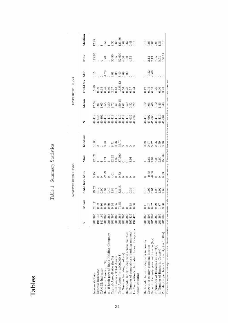
capital-asset ratio of 9.23 %. Differences between diversified and nondiversified

banks are shown in Table 1. The majority of bank-year observations (about 83

%) are from nondiversified banks. This also reflects the fact that only 6 % of all

banks were diversified in 1978, whereas almost half of all banks in 2006 had at least

branches in two counties. Moreover, Table 1 suggests that diversified banks tend to

be (a) less risky, (b) larger, and (c) have lower capital-asset ratios.

10

3.2 Results

All regression models include bank fixed effects, which implies that the estimated

coefficient represents within bank changes in their risk taking behavior as a bank’s

competitors’ become more diversified than banks. Standard errors are robust and

clustered at the bank level. Results are presented in Table 2 and indicate that a

bank’s risk taking is negatively related to differences in the diversification of bank i

and its competitors even without conditioning on bank or macroeconomic controls.8

Moreover, the effect is significant at the 1 % level and robust to the inclusion of

bank and macroeconomic controls (column 2 and 3). Thus, banks tend to be less

risky if they are less diversified than their competitors even if I control for compet-

itive aspects of the banking market. Particularly, the estimated coefficient on the

Herfindahl Index of deposits is positive and significant, which indicates that banks

located in counties with a greater concentration of deposits across banks tend to be

riskier. This is consistent with theories arguing that less competition is associated

with greater bank risk taking (Boyd and de Nicolo, 2005).

The first two regression models include year fixed effects to account for unob-

servable time trends. However, these fixed effects only capture unobservable time-

varying effects at the country level. Therefore I include region specific (column 4) or

state-specific time dummies (column 5) to capture unobservable time-varying effects

on banks’ risk taking at the region or state level.9 In particular, the state-specific

time dummies capture unobservable effects such as changes in the competitive en-

vironment of commercial banks at the state level. The relationship between banks’

diversification and risk taking is significant at the 1 % level in all regression models.

To examine whether the results are sensitive to the definition of risk taking, I

8Since Inverse Z-Score is small, I multiply it by 1,000 for my analysis.9The regions are Midwest (IA, IL, IN, KS, MI, MN, MO, ND, NE, OH, WI), Northeast (CT,

MA, MD, ME , NH, NJ, NY, PA, RI, VT, WV), South (AL, AR, DC, FL, GA, KY, LA, MS, NC,OK, SC, TN, TX, VA) and West (AZ, CA, CO, ID, MT, NM, NV, OR, UT, WA, WY).

11

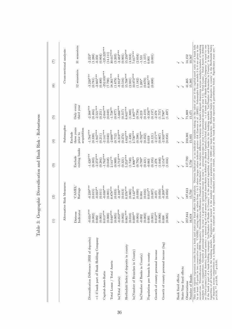
repeat the analysis using the Distress Indicator or ‘CAMEL’ ratings as dependent

variable. I also include state-year fixed effects to account for unobservable charac-

teristics that vary within a state. Regression results are presented in Table 3 and

confirm the earlier findings as the results suggest that a bank’s risk taking is lower

when competitors become more diversified. Several banks exit the sample due to

mergers and acquisitions or failures. Although I include bank fixed effects in the

analysis, it is possible that a weeding out of risky banks (Carlson and Mitchener

(2009)) affects my findings. Therefore, I estimate the relationship between risk

taking and diversification excluding all banks that fail, merge or become acquired

during the sample period. The earlier findings are not driven by this and are robust

to this sample restriction. Similarly, banks also engage in mergers and acquisitions

during the sample period. This also affects the regression results, particularly In-

verse Z-Score, as a merger or acquisition leads to a re-evaluation of banks’ balance

sheets. To account for this, I exclude observations up to three years before a bank’s

merger and/or acquisition (column 4). The findings are robust to that sample se-

lection. Due to construction, Inverse Z-Score is correlated over time, as I use the

previous five semesters to estimate the volatility of bank profits. Hence, Inverse

Z-Score in year t uses information on profits that are also used for the computation

of Inverse Z-Score in year t − 1. Moreover, persistence in earnings might also con-

tribute to a potential serial correlation of my risk measure. To address this, and

virtually eliminate all autocorrelation due to construction, I restrict the sample and

only include every third year in the estimation in column 5. The results are robust

to this exclusion. To further examine the robustness of this finding, I collapse the

data into 6 (2) equal periods of 12 (31) semesters and compute the average value of

each variable for each cross-sectional period in column 6 (7).10 Since I am interested

in within bank changes in risk taking as the diversification between a bank and its

10To construct Inverse Z-Score for each time period, I compute the volatility of profits andaverage ROA over each time period.

12

competitors changes, I need at least two observations for each bank and therefore

cannot collapse the data over the whole sample period and conduct a cross sectional

analysis. In all robustness tests I find that a bank’s risk taking is lower when it is

less diversified than its competitors.11

To translate these findings into a likelihood of failing, I estimate how a bank’s

probability of failing is related to Inverse Z-Score. Using information on the bankruptcy

of 1,152 bank failures during the sample period, I estimate a state and year fixed

effects logit regression and compute the average marginal effect of a one unit change

in Inverse Z-Score on a bank’s failure likelihood. Estimations from this logit model

suggest that a one unit increase in Inverse Z-score decreases the likelihood of failing

by approximately 1.2 %-points. Using the coefficient from column 4 in Table 2, I

find that if the difference between a bank’s competitors’ diversification and the di-

versity of a bank increases by one standard deviation, then the probability of failure

for a bank decreases by 0.7 basis points. During the sample period, on average three

out of a thousand banks fail each year, and so this implies that the average annual

failure rate would be reduced by approximately 2 %. This is a rather small effect.

However, it is a net effect and does not reflect the causal impact of diversification on

risk taking since causality is not identified in this Ordinary-least squares estimation.

3.2.1 Dynamic effects

In 1976 about 8 % of all banks in the sample have branches in more than one county.

In 2006, on the other hand, almost every second bank has a branch network that

spans at least two counties (Figure 1). To examine the dynamic effects of risk taking

11The estimated coefficient on the difference in diversification in column 7 is significant at the 8%-level.

13

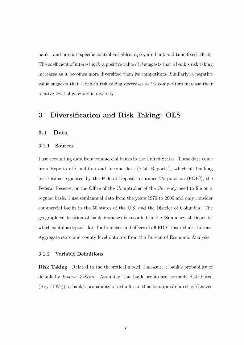
as competitors expand, I estimate the following regression model:

Ri,t = αi + αt +10∑

p=−10

βpYp,t +X’i,s,tρ+ εi,t

where Ri,t is the Inverse Z-Score of bank i in year t, Yp,t is a dummy variable

that takes on the value of one if in year t, bank i’s competitors diversify their

branch network across markets in p years. The effect on risk taking in the year

of the competitors’ expansion is dropped due to collinearity. Thus the coefficients

βp are relative to the year of competitors’ expansion. Figure 2 plots the estimated

coefficients βp as well as the 95 % confidence interval for these coefficients. To

account for a bank’s own diversification activity I restrict attention to banks that

are only active in a single market.

Figure 2 shows that a bank’s risk taking decreases once its competitors expand

their branch network into more markets. Furthermore, the figure shows that risk

taking does not significantly change before a competitor expands, and only decreases

significantly two years after a competitors expansion. This lagged response can

partly be attributed to the fact that Inverse Z-Score is smoothed as it is computed

using information from earlier years. The pattern in Figure 2 also shows that a

bank’s risk taking stays significantly lower once competitors diversified their branch

network into more markets, suggesting that the expansion of competitors has an

effect on a bank’s risk taking behavior.

3.2.2 Own Diversification vs. Competitors’ Diversification

The results so far examine how bank risk taking is related to changes in the relative

difference in geographic diversification of a bank and its competitors. It is also

possible to differentiate this effect further. In particular, I examine whether this

effect is different if (a) a bank is more diversified than its competitors, or (b) a bank

14

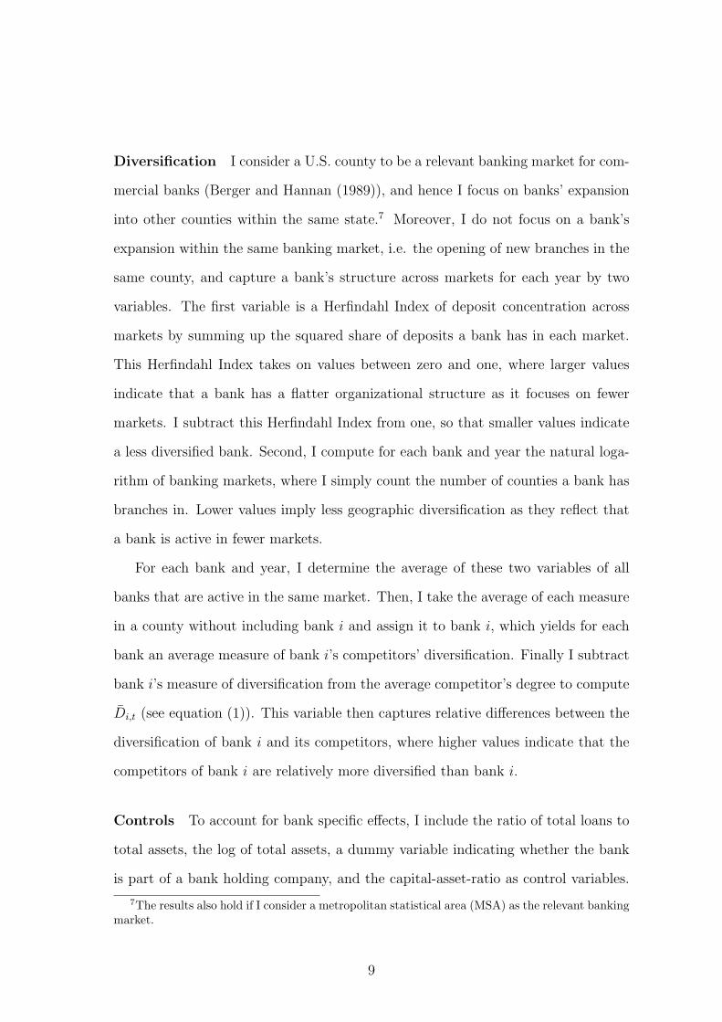
is less than diversified than its competitors. Therefore, I estimate the following

regression model:

Ri,t = αi + αt +e=3∑e=1

βeOi,e,t +e=3∑e=1

γeCi,e,t +X’i,tρ+ εi,s,t (2)

where Ri,t is the Inverse Z-Score of bank i in year t, Oi,e (Ci,et) is a dummy variable

that takes on the value of one if the relative difference in diversification between

bank i and its competitor is positive (negative), and in the highest, medium or

lowest sample tercile compared to the case where a bank and its competitors are

not diversified. For example, β3 reflects the difference in risk taking if bank i is

more diversified than its competitors and the diversification difference is in the

highest sample tercile. Similarly, γ3 captures the difference in risk taking if bank

i’s competitors are more diversified that bank i and this difference is in the highest

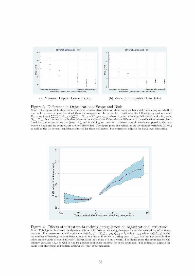
sample tercile. The estimated coefficients are plotted in Figures 3(a) and 3(b), and

show that a bank’s risk taking is lower when it is less diversified than its competitors,

but is higher when it is more diversified than its competitors. Interestingly, this effect

changes sign when both banks are equally diversified.

4 The Effect of Diversification on Risk Taking:

2SLS

Ordinary-least squares estimation does not allow an identification of the causal re-

lationship between the effects of diversification on risk because of, for instance,

influences that jointly affect bank risk taking and diversification. To address this

concern, I employ two instrumental variable strategies. The first strategy uses the

timing of intrastate branching deregulation at the state level as an excluded in-

strument for the diversification activity of banks. The second approach combines

15

the timing of intrastate branching deregulation, the distance between a bank and

counties within a state and bank specific characteristics to develop an instrumental

variable at the bank level.

4.1 Intrastate Branching Deregulation as a Natural Exper-

iment

Banks in the United States were restricted in their branching decision within and

across states for many decades. Limits on the location of branch offices were imposed

in the 19th century, and were supported by the argument that allowing banks to

expand freely could lead to a monopolistic banking system. The granting of bank

charters was also a profitable income source for states, increasing incentives for

states to enact regulatory policies.12 These regulations led to a banking system that

was characterized by local monopolies within states since geographical restrictions

prohibited other banks from entering a market. Because banks were beneficiaries of

this regulation, they also had an incentive to preserve the status quo (Kroszner and

Strahan, 1999).

With the emergence of new technologies - such as the Automated Teller Machines

and more advanced credit scoring techniques - banks’ benefits from regulation de-

clined. Eventually intrastate branching restrictions were lifted in states, and banks

were allowed to branch freely within a state. The passage of the Riegle-Neal Act in

1994 by U.S. Congress finally removed all remaining barriers by the middle of the

1990s.13

12How severe these restrictions were shows the case of Illinois: before the removal of theserestrictions, the state allowed banks to only open two branches within 3,500 yards of its mainoffice (Amel and Liang, 1992).

13Previous research on intrastate branching deregulation suggests that the removal of branchingrestrictions had significant effects on the real activity and economic development. See among othersJayaratne and Strahan, 1996, Beck et al., 2010. Dates for each state are given in Table A.II.

16

The first stage regression model is given as:

D̄i,t = αi + αt + γZi,s,t +X’i,s,tρ+ εi,t, (3)

where D̄i,t is the relative level of geographic diversity between bank i and its com-

petitors, and larger values of D̄i,t indicate that competing banks are more diversified

than bank i; Zi,s,t is an instrumental variable at the (1) state- or (2) bank-level, based

on the removal of intrastate branching restrictions; X’i,s,t is a vector of bank-, and

or state-specific control variables; αi/αt are bank and time fixed effects.

In the second stage, I use the predicted value of D̄i,t to determine how it impacts

a banks’ risk taking.

Ri,t = β ˆ̄Di,t +X’i,s,tγ + δ̃i + δ̃t + ηi,s,t, (4)

where ˆ̄Di,t is the predicted value of the relative level of diversification between a bank

and its competitors from the first stage regression. I use the same data sources as

in the earlier analysis. Following previous research on intrastate branching deregu-

lation, I drop Delaware and South Dakota from the analysis since the structure of

the banking system in these states was heavily affected by other laws. Therefore it

is not possible to isolate the effect of intrastate branching deregulation in these two

states.

4.2 State-level instruments

4.2.1 Intrastate Branching Deregulation and Diversification

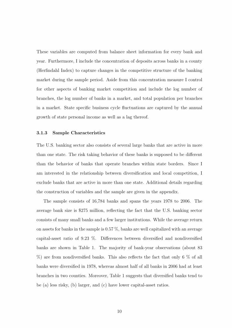
Intrastate branching restrictions prohibited banks from expanding their branch net-

work for many years. Figure 4 shows the dynamic effects of intrastate branching

deregulation in a state on the log number of markets a bank is active in. In partic-

17

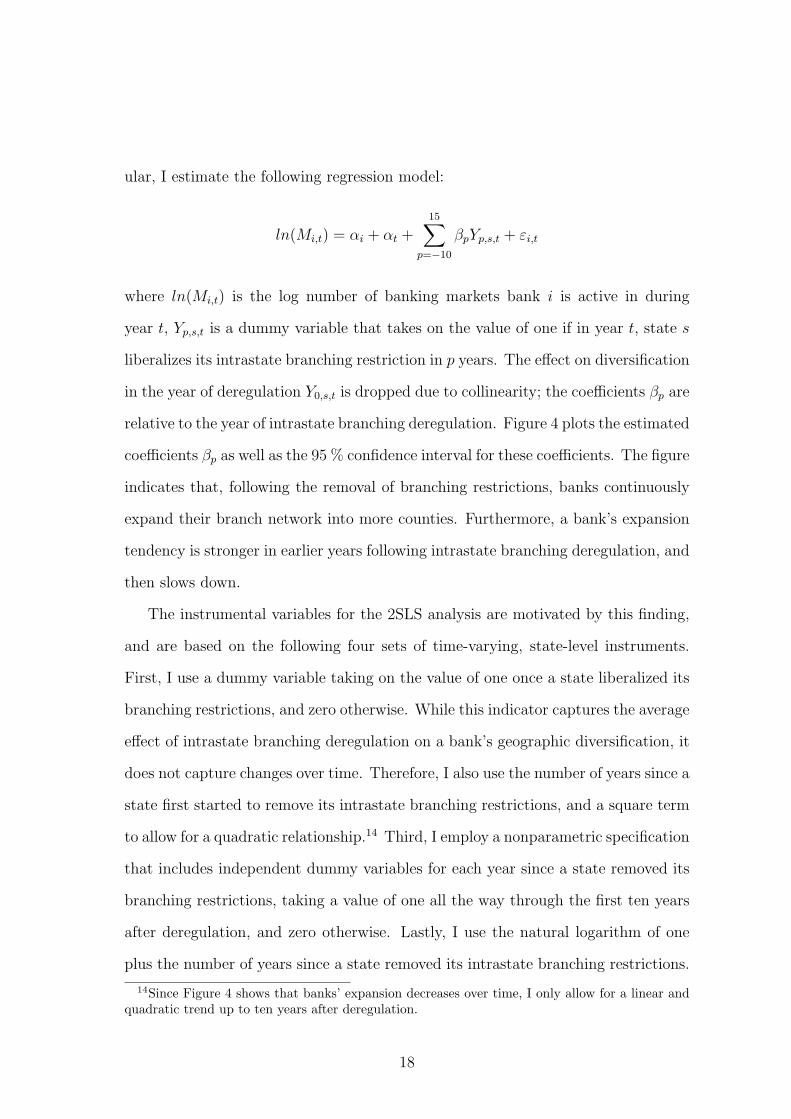
ular, I estimate the following regression model:

ln(Mi,t) = αi + αt +15∑

p=−10

βpYp,s,t + εi,t

where ln(Mi,t) is the log number of banking markets bank i is active in during

year t, Yp,s,t is a dummy variable that takes on the value of one if in year t, state s

liberalizes its intrastate branching restriction in p years. The effect on diversification

in the year of deregulation Y0,s,t is dropped due to collinearity; the coefficients βp are

relative to the year of intrastate branching deregulation. Figure 4 plots the estimated

coefficients βp as well as the 95 % confidence interval for these coefficients. The figure

indicates that, following the removal of branching restrictions, banks continuously

expand their branch network into more counties. Furthermore, a bank’s expansion

tendency is stronger in earlier years following intrastate branching deregulation, and

then slows down.

The instrumental variables for the 2SLS analysis are motivated by this finding,

and are based on the following four sets of time-varying, state-level instruments.

First, I use a dummy variable taking on the value of one once a state liberalized its

branching restrictions, and zero otherwise. While this indicator captures the average

effect of intrastate branching deregulation on a bank’s geographic diversification, it

does not capture changes over time. Therefore, I also use the number of years since a

state first started to remove its intrastate branching restrictions, and a square term

to allow for a quadratic relationship.14 Third, I employ a nonparametric specification

that includes independent dummy variables for each year since a state removed its

branching restrictions, taking a value of one all the way through the first ten years

after deregulation, and zero otherwise. Lastly, I use the natural logarithm of one

plus the number of years since a state removed its intrastate branching restrictions.

14Since Figure 4 shows that banks’ expansion decreases over time, I only allow for a linear andquadratic trend up to ten years after deregulation.

18

To isolate the effect of a bank’s own expansion activity during the sample period,

I restrict attention to observations where banks are not diversified and therefore only

operate branches in one county. This allows me to identify the effect of competitors’

expansion on a bank’s risk taking, but also excludes large banks from the sample as

nondiversified banks are small.15 Because I only consider nondiversified banks for

this analysis, ˆ̄Di,t is measured relative to a nondiversified bank i and thus captures

the diversification activity of bank i’s competitors. Furthermore, I exclude observa-

tions up to three years before a bank’s merger or acquisition to account for changes

in Inverse Z-Score due to merger activity. First stage regression results of these

instruments on competitors’ expansion across markets are presented in Panel B of

Table 4. Similar to Figure 4, results in Table 4 indicate that intrastate branching

deregulation is associated with an increase in the diversification of banks as mea-

sured by the Herfindahl Index of deposits across banking markets (columns 1 to

4). This also holds when I measure a bank’s diversification using the log number

of markets a bank is active in (columns 5 to 8). The associated F-statistics sup-

port the use of these instruments as F-test results show that intrastate branching

deregulation significantly impacts the expansion of banks.

4.2.2 Diversification and Risk Taking: Second-stage

As mentioned before, the measure of relative diversification reflects changes in a

competitors degree of geographic diversity since I restrict attention to banks that

are not geographically diversified in this analysis. Panel A of Table 4 reports second

stage results of a 2SLS regression of bank risk on the level of geographic diversifica-

tion of competing banks, as measured by the competitor’s average dispersion across

markets (columns 1 to 4), or the average number of markets competitors are active

15Nondiversified banks have an average size of $71 million (see Table 1). In the second identi-fication strategy (Section 4.3), however, I include all (diversified and nondiversified) banks sinceI use an instrumental variable at the bank-level and therefore control for a bank’s own expansionactivity.

19

in (columns 5 to 8).

The results indicate that bank risk decreases significantly when competitors ex-

pand their diversification across markets. This effect is not sensitive to the defini-

tion of banks’ diversification, since I also find a statistically significant relationship

between competitors’ diversification and risk when I use the number of markets,

competitors are active in (columns 5 to 8). 16 Compared to the OLS results (Table

2), the estimated coefficients from the 2SLS analysis are larger in magnitude, sug-

gesting an attenuation bias due to reverse causality which results in smaller OLS

estimates. The instrumental variables, however, allow me to identify a causal impact

of changes in competitors’ diversification on banks’ risk taking.

Using the estimated coefficient reported in column 4 of Panel A of Table 4, I

compute that if competitors increase their dispersion across markets by one stan-

dard deviation, a bank’s probability of failure decreases by about 6 basis points.

Since the average annual failure rate of banks is 30 basis points, this implies that

a bank’s annual risk of bankruptcy decreases by 20 % when competitors increase

their diversity by one standard deviation.

4.3 Bank-level instruments

Instrumental variables at the state-level are not able to capture a bank’s decision

to expand into other markets, and hence only provide an instrument for the aver-

age expansion of banks within a state. Moreover, unobservable state specific time

varying effects, such as a state’s overall level of bankruptcy risk, might influence my

findings.

Therefore, I design a strategy to differentiate the effect of a removal of branching

restrictions on banks’ expansion, which allows me to (1) account for the endogenous

16Moreover, I also find that the effect between competitors’ diversification and risk taking is notsensitive to the definition of risk since I find a statistically significant relationship between risktaking and diversification when I measure risk taking using the Distress indicator or ‘CAMEL’ratings. These results are unreported and are available upon request.

20

choice of banks to expand within a state, and (2) include state specific time fixed ef-

fects to capture unobservable changes within a state. This approach incorporates (a)

the timing of intrastate branching deregulation at states, (b) the distance of coun-

ties within a state, and (c) differences between banks in regards to their regulatory

charter and/or membership to the Federal Reserve System.

4.3.1 Empirical Strategy

To comply with intrastate branching restrictions, banks were often not allowed to

expand into areas that exceed a certain distance from its main office. For instance,

the state of Illinois only allowed banks to open two branches within 3,500 yards

of its main office prior to the removal of branching restrictions (Amel and Liang,

1992). The possibility to expand only within a certain range of the bank’s main

office significantly limited a bank’s lending activities, especially since informational

asymmetries between borrowers and lenders are intensified as distance between bor-

rowers and lenders increases (Berger et al., 2005, Petersen and Rajan, 2002). Due

to branching restrictions a bank’s activity within states was mainly determined by

the location of a its main office. Once states removed their branching restrictions,

however, distance to other counties is supposed to be less important as banks were

not tied to certain geographic areas by regulation.

To incorporate the effect of distance on banks’ expansion behavior before and

after the removal of intrastate branching restrictions, I construct a bank-specific

instrumental variable, based on the timing of intrastate branching deregulation, the

distance of counties within a state, and bank specific characteristics. Specifically,

I estimate the effect of distance of a bank’s home county and another county on

the degree of a bank’s expansion into that county. Furthermore, I estimate how

that effect changes once states remove their intrastate branching restrictions. In

particular, I hypothesize that a bank’s share of deposits is larger in counties that

21

are closer to the bank’s home county. Moreover, I expect that the effect of distance

on a bank’s expansion into another county decreased once states removed intrastate

branching restrictions.

Additionally, I examine how the relationship between expansion and distance

is different across bank types. In particular, I hypothesize that the link between

expansion and distance differs by (1) a bank’s charter authority (state or national

charter) and (2) a bank’s membership to the Federal Reserve System. Because

of the McFadden Act of 1927 and the Banking Act of 1933, banks in the U.S.

are subject to state specific banking laws irrespective of their charter type. Aside

from smaller differences, a bank’s charter choice determines its primary regulatory

agency, which can be associated with additional costs: state chartered banks are

supervised by state banking regulators and do not need to bear any costs due to

supervision. National chartered banks, on the other hand, are supervised by the

Office of the Comptroller of the Currency (OCC), which charges supervisory fees

(Blair and Kushmeider (2006)). Anecdotal evidence also suggests, that banks choose

state charters because state regulators, in contrast to national regulators, have a

better understanding of a bank’s business model in light of the local economy.17

Hence, a bank’s charter choice is supposed to reflect its desire to expand within

state borders once states liberalize intrastate branching restrictions.

Aside from this, banks can also decide whether they want to become members

of the Federal Reserve System. While national chartered banks are members of

the Federal Reserve System by default, state chartered banks can apply for mem-

bership. The Federal Reserve bank of the bank’s district decides whether to grant

membership, and evaluates the bank’s application based on factors such as, financial

condition or general character of management. Membership to the Federal Reserve

System provides banks with additional benefits, such as, the privilege of voting for

17See for instance http : //www.arkansas.gov/bank/benefits why.html

22

directors of the Federal Reserve bank. However, membership to the Federal Re-

serve System is also costly, as it requires banks to subscribe to the capital stock in

the Federal Reserve bank of its district. Moreover, once state chartered banks are

members of the Federal Reserve System, they are jointly supervised by the Federal

Reserve and state banking regulators - although at no additional costs.

Given these differences across bank types, I hypothesize that a removal of branch-

ing restrictions has different effects on banks’ branching decisions. Compared to

state chartered banks, I hypothesize that the effect of distance on expansion changes

more for national chartered banks once states remove their branching restrictions.

Similarly, I hypothesize that - compared to non-member banks - member banks of

the Federal Reserve System have a greater incentive to expand once states liberalize

their branching restrictions, implying that distance becomes less important once

branching restrictions are removed.

4.3.2 Expansion, Intrastate Branching Deregulation and Distance

To examine the effect of distance and size on the expansion of banks within state

borders before and after intrastate branching deregulation, I estimate the following

distance-deregulation zero-stage:

Sharei,h,c,t = α1 ln(disth,c) + α2 ln(disth,c)×Bi,t +

+ α3 ln(disth,c)×Bi,t × Ii + α4 ln(disth,c)× Ii +∆i,h,c,t + εi,h,c,t,

where Sharei,h,c,t is the share of deposits bank i, headquartered in county h,

holds in branches in county c in year t; disth,c is the distance (in miles) between

county h and county c; Bi,t is a dummy variable taking on the value of one whether

bank i’s state removed its intrastate branching restrictions, or zero otherwise; Ii is

an indicator variable taking on the value of one, (1) whether bank i had a national

23

charter prior to intrastate branching deregulation, (2) and/or was a member of the

Federal Reserve System prior to intrastate branching deregulation, or zero otherwise;

∆i,h,c,t is a set of dummy variables accounting for fixed effects at the bank, county

and year level.

The baseline effect of distance on banks’ expansion is captured by the coefficient

α1. Changes of this relationship due to a removal of intrastate branching restrictions

are reflected in α2. Differential effects because of banks’ charter type or their mem-

bership to the Federal Reserve System are captured by α3. As mentioned above,

I hypothesize that banks have less deposits in branches that are further away, i.e.

α1 < 0, but I expect this effect to be mitigated once states liberalize branching

restrictions, i.e. α2 > 0. Furthermore, I expect that the effect of distance on ex-

pansion decreases more for national banks or Federal Reserve member banks once

states remove intrastate branching prohibitions.

Table 5 presents results from an OLS estimation where I use the share of deposits

in % points as the dependent variable.18 The results show that banks have a smaller

share of deposits in counties that are further away from the county where they are

headquartered in. As hypothesized, the effect of distance on the share of deposits

becomes smaller once states remove their branching restrictions. This also holds

when I include bank fixed effects (column 2). In columns (3) and (4), I include the

aforementioned bank specific variables. Results in Table 5 suggest that distance is

less important for a bank’s expansion if the bank is a member of the Federal Reserve

System and/or has a national charter.

The bank specific heterogeneity in the effect of distance on banks’ expansion

within states allows me to construct a projected expansion for each bank and year.

To construct bank-level instruments consistent with my earlier analysis, I use as

dependent variable (1) an indicator taking on the value of one whether bank i has

18Due to the size of the data set, I demeaned the dependent and independent variables by handto capture the reported fixed effects. Standard errors are robust and clustered at the bank level.

24

a branch in county c in year t, and (2) the squared share of deposits bank i holds

in county c in year t. The projected variables are then aggregated at the bank-

year level to construct instrumental variables for (1) a bank’s number of active

banking markets, and (2) a bank’s deposit dispersion across markets. Similar to

before, I construct instruments for competitors’ expansion by taking the average of

each variable in a county without including bank i and assigning it to bank i and

calculate the projected relative difference in the degree of geographic diversity by

the difference between these two values.

4.3.3 Diversification and Risk Taking: Second-stage

Table 6 presents second stage regression results using instrumental variables based

on the distance-deregulation zero-stage. In particular, I use the model of column 4

in Table 5 to construct instruments for a bank’s level of geographic diversity and the

diversity of its competitors. Since this instrument varies at the bank-level, I include

all bank-year observations in my analysis.

Consistent with earlier findings, results in Table 6 indicate that banks’ risk taking

decreases when the relative difference in diversification between banks and their

competitors increases. This is not sensitive to the definition of diversification as I

find a statistically significant effect between diversification and risk taking when I

use the difference between a bank’s dispersion of deposits across counties and the

deposit dispersion of a bank’s competitors’ (column 1) or the difference in their

number of markets (column 2).

Because this approach provides an instrumental variable at the bank level, I

can separately identify (a) the impact of a bank’s own level of diversification on

its risk taking behavior and (b) the impact of a bank’s competitors’ changes in

diversification on risk taking. The findings in Table 6 suggest that risk taking

significantly increases when a bank diversifies its activity across markets, consistent

25

with earlier work by Demsetz and Strahan (1997). However, when competitors

increase their level of diversification across counties, a bank’s risk taking significantly

decreases. This finding is not sensitive to the definition of diversification as it also

holds when I use the number of markets, a bank is active in to capture its degree of

diversification. Furthermore, I also include state-year fixed effects in Table 6. These

fixed effects capture unobservable, time-varying changes at the state level and hence

account for other confounding effects at the state level, such as changes in overall

bankruptcy risk at the state.

5 Conclusion

I hypothesize that the diversification activity of banks not only affects their risk

taking, but also the risk taking of competing, nondiversified banks. In addition to

theories of competition and bank risk taking, the expansion of banks has an impact

on risk taking as it changes their behavior which also impacts the lending decisions

of competing banks due to competition for borrowers in the market. Furthermore,

the diversification of banks can lead to an increase or decrease of competing banks’

risk taking behavior.

To examine this empirically, I analyze the relationship between diversification

and risk taking using data from U.S. commercial banks. I find evidence consistent

with this notion as the risk taking behavior is different between diversifying and

nondiversifying banks. OLS regression results indicate that the level of competitors’

degree of diversification is significantly correlated with a bank’s risk taking behavior,

even when I control for changes in the competition for borrowers. Moreover, I use the

staggered timing of intrastate branching deregulation, and a distance-deregulation

model to pin down the causal relationship of banks’ diversification on risk taking of

competing banks. Regression results indicate that banks decrease risk taking when

26

competitors increase their branch network across counties or when their dispersion

of deposits across markets changes. My results also indicate that a bank’s own risk

taking increases when it diversifies across markets. Hence, these findings suggest

that there are indirect effects of diversification, as a bank’s risk taking is also af-

fected as competitors change their diversification.

27

References

Allen, F. and D. Gale (2000): Comparing Financial Systems, MIT Press.

Amel, D. and N. Liang (1992): “The Relationship between Entry into Banking

Markets and Changes in Legal Restrictions on Entry,” Antitrust Bulletin, 631 –

649.

Beck, T., R. Levine, and A. Levkov (2010): “Big Bad Banks: The Winners

and Losers from Bank Deregulation in the United States,” Journal of Finance,

65, 1637 – 1667.

Berger, A. N. and T. H. Hannan (1989): “The Price-Concentration Relation-

ship in Banking,” The Review of Economics and Statistics, 291 – 299.

Berger, A. N., N. H. Miller, M. A. Petersen, R. G. Rajan, and J. C.

Stein (2005): “Does function follow organizational form? Evidence from the

lending practices of large and small banks,” Journal of Financial Economics, 76,

237–269.

Blair, C. E. and R. M. Kushmeider (2006): “Challenges to the Dual Banking

System: The Funding of Bank Supervision,” FDIC Banking Review, 18, 1 – 22.

Boyd, J. H. and G. de Nicolo (2005): “The Theory of Bank Risk Taking and

Competition Revisited,” Journal of Finance, 60, 1329–1343.

Boyd, J. H., G. de Nicolo, and A. M. Jalal (2007): “Bank Risk-Taking and

Competition Revisited: New Theory and New Evidence,” IMF working paper

WP/06/297.

——— (2009a): “Bank Competition, Asset Allocations and Risk of Failure: An

Empirical Investigation,” CesIfo working paper 3198.

28

——— (2009b): “Bank Competition, Risk and Asset Allocations,” IMF working

paper WP/09/143.

Boyd, J. H., G. de Nicolo, and E. Loukoianova (2009c): “Banking Crises

and Crisis Dating: Theory and Evidence,” IMF working paper WP/09/141.

Calomiris, C. W. and J. R. Mason (2000): “Causes of U.S. Bank Distress

during the depression,” NBER working paper 7919.

Carlson, M. and K. J. Mitchener (2009): “Branch Banking as a Device for

Discipline: Competition and Bank Survivorship during the Great Depression,”

Journal of Political Economy, 117, 165–210.

de Nicolo, G. (2000): “Size, charter value and risk in banking: an international

perspective,” Board of Governors of the Federal Reserve System, International

Finance Discussion Paper No.689.

Demsetz, R. S. and P. E. Strahan (1997): “Diversification, Size, and Risk at

Bank Holding Companies,” Journal of Money, Credit, and Banking, 29, 300–313.

Diamond, D. (1984): “Financial intermediation and delegated monitoring,” Review

of Economic Studies, 51, 393–414.

Goetz, M. R., L. Laeven, and R. Levine (2011): “The Valuation Effects of

Geographically Diversified Bank Holding Companies: Evidence from U.S. Banks,”

NBER Working Paper No. 17660.

Hertzberg, A., J. M. Liberti, and D. Paravisini (2010): “Information and

Incentives Inside the Firm: Evidence from Loan Officer Rotation,” Journal of

Finance, 65, 795–828.

29

Jayaratne, J. and P. E. Strahan (1996): “The Finance-Growth Nexus: Ev-

idence from Bank Branch Deregulation,” Quarterly Journal of Economics, 111,

639–670.

Jimenez, G., J. A. Lopez, and J. Saurina (2010): “How does Competition

Impact Bank Risk-Taking?” Mimeo, Banco de Espana.

Keeley, M. C. (1990): “Deposit Insurance, Risk, and Market Power in Banking,”

American Economic Review, 80, 1183–1199.

Kroszner, R. S. and P. E. Strahan (1999): “What Drives Deregulation? Eco-

nomics and Politics of the Relaxation of Bank Branching Restrictions,” Quarterly

Journal of Economics, 114, 1437–1467.

Laeven, L., P. Bongini, and G. Majnoni (2002): “How Good is the Market at

Assessing Bank Fragility? A Horse Race Between Different Indicators,” Journal

of Banking and Finance, 26, 1011–1028.

Laeven, L. and R. Levine (2009): “Bank governance, regulation and risk tak-

ing,” Journal of Financial Economics, 93, 259–275.

Liberti, J. M. and A. R. Mian (2009): “Estimating the Effect of Hierarchies on

Information Use,” The Review of Financial Studies, 22, 4057–4090.

Martinez-Miera, D. and R. Repullo (2010): “Does Competition Reduce the

Risk of Bank Failure?” Review of Financial Studies, 23, 3638–3664.

Mitchener, K. J. (2005): “Bank Supervision, Regulation, and Instability During

the Great Depression,” The Journal of Economic History, 65, 152–185.

Morgan, D. P., B. Rime, and P. E. Strahan (2004): “Bank Integration and

State Business Cycles,” Quarterly Journal of Economics, 1555–1584.

30

Petersen, M. A. (2004): “Information: Hard and Soft,” Mimeo.

Petersen, M. A. and R. G. Rajan (2002): “Does Distance Still Matter? The

Information Revolution in Small Business Lending,” Journal of Finance, 57, 2533–

2570.

Roy, A. (1952): “Safety First and the Holding of Assets,” Econometrica, 431–449.

Scharfstein, D. S. and J. C. Stein (2000): “The Dark Side of Internal Capital

Markets: Divisional Rent-Seeking and Inefficient Investment,” Journal of Finance,

55, 2537–2564.

Stein, J. C. (2002): “Information Production and Capital Allocation: Decentral-

ized versus Hierarchical Firms,” Journal of Finance, 57, 1891–1921.

31

Figures

92.11

4.5311.349 .6245 .3454 .2126 .1927 .1196 .0465 .4717

020

4060

8010

0P

erce

nt

0 2 4 6 8 10Banking Markets

1976

(a) 1976

53.34

22.54

10.18

4.6622.319 1.6 .8191 .6804 .5166

3.339

020

4060

8010

0P

erce

nt

0 2 4 6 8 10Banking Markets

2006

(b) 2006

Figure 1: Distribution of Banks by Number of Counties ServedThis figure shows the distribution of U.S. commercial banks by the number of counties in which they are active infor 1976 and 2006.

−4

−2

02

4E

ffect

on

Ris

k

−10 −5 0 5 10Year since Competitor’s Expansion

Diversification and Risk

Figure 2: Effects of Competitor’s Expansion on Risk TakingNote: This figure illustrates the dynamic effects of a competitor’s expansion on a bank’s risk taking. The regressionmodel is given as Ri,t) =

∑10p=−10 αpYp,i,t+ δ̃i+ δ̃t+τi,s,t where Ri,t) is the Inverse Z-Score of bank i in year t, Yp,i,t

is a dummy variable that takes on the value of one if in year t the competitor of bank i expands its branch networkin p years. The figure plots the estimates on the dummy variables (αp) as well as the 95 percent confidence intervalfor these estimates. Only banks that are active in one market are considered for this analysis. The regression adjustsfor bank-level clustering and centers around the year of expansion. Coefficients at the end points (α−10, α+10) areomitted.

32

−1

01

23

Effe

ct o

n R

isk

competitor less diversified competitor more diversified Competitors’ Diversification − Own Diversification

Diversification and Risk

(a) Measure: Deposit Concentration)

−2

02

46

Effe

ct o

n R

isk

competitor less diversified competitor more diversified Competitors’ Diversification − Own Diversification

Diversification and Risk

(b) Measure: ln(number of markets)

Figure 3: Difference in Organizational Scope and RiskNote: This figure plots differential effects of relative diversification differences on bank risk depending on whetherthe bank is more or less diversified than its competitors. In particular, I estimate the following regression model:Ri,t = αi +αt +

∑e=3e=1 βeOi,e,t +

∑e=3e=1 γeCi,e,t +X’i,tρ+ εi,s,t, where Ri,t is the Inverse Z-Score of bank i in year t,

Oi,e (Ci,et) is a dummy variable that takes on the value of one if the relative difference in diversification between banki and its competitor is positive (negative), and in the highest, medium or lowest sample tercile compared to the casewhere a bank and its competitors are not diversified. The figure plots the estimates on the dummy variables (βe/γe)as well as the 95 percent confidence interval for these estimates. The regression adjusts for bank-level clustering.

−.0

50

.05

.1.1

5.2

ln(N

umbe

r of

act

ive

mar

kets

)

−10 −5 0 5 10 15Years before/ after intrastate branching deregulation

Figure 4: Effects of intrastate branching deregulation on organizational structureNote: This figure illustrates the dynamic effects of intrastate branching deregulation on the natural log of bankingmarkets. The regression model is given as ln(Mi,s,t) =

∑15p=−10 αpYp,s,t + δ̃i + δ̃t + τi,s,t where ln(Mi,s,t) is the

log number of banking markets bank i, located in state s, is active in during year t, Yp,s,t is a dummy variable thattakes on the value of one if in year t deregulation in a state s is in p years. The figure plots the estimates on thedummy variables (αp) as well as the 95 percent confidence interval for these estimates. The regression adjusts forbank-level clustering and centers around the year of deregulation.

33

Tab

le1:

SummaryStatistics

Nondiversified

Banks

Diversified

Banks

NM

ean

Std

.Dev.M

inM

ax

Median

NM

ean

Std

.Dev.M

inM

ax

Median

Inverse

Z-Sco

re206,365

23.17

19.52

3.15

120.21

16.83

46,419

17.69

15.56

3.15

119.95

12.98

DistressIndicator

196,145

0.02

0.12

01

042,046

0.01

0.09

01

0CAMEL-Indicator

140,166

0.86

0.90

04

140,803

1.05

0.93

04

1Return

onAssets(in%)

206,365

0.58

0.34

-2.29

1.71

0.58

46,419

0.55

0.28

-1.79

1.70

0.54

=1ifbankpart

ofBankHoldingCompany

206,365

0.60

0.49

01

146,419

0.80

0.40

01

1Capital-Asset-R

atio(in%)

206,365

9.34

2.84

4.01

32.42

8.71

46,419

8.72

2.37

4.01

30.90

8.30

TotalLoans/TotalAssets

206,365

0.55

0.14

01.32

0.56

46,419

0.61

0.13

0.08

1.05

0.63

TotalAssets(in1,000,000$)

206,365

74.51

331.81

0.72

37,700

36.70

46,419

450.15

1,585.12

3.49

52,600

123.86

ln(N

umber

bankingmarkets)

206,365

00

00

046,419

1.01

0.54

0.69

4.36

0.69

HerfindahlIndex

ofdep

osits

across

counties

206,365

00

00

046,419

0.59

0.28

0.00

1.00

0.62

ln(N

umber

ofco

mpetitor’sbankingmarkets)

197,425

0.18

0.34

03.91

041,632

0.52

0.57

04.73

0.41

1-Competitor’sHerfindahlIndex

ofdep

osits

across

counties

197,425

0.08

0.16

01

041,632

0.22

0.24

01

0.16

HerfindahlIndex

ofdep

osits

inco

unty

206,365

0.11

0.13

01

0.08

46,419

0.12

0.12

01

0.10

Growth

ofco

unty

personalinco

me

205,505

0.07

0.07

-0.68

2.64

0.07

45,602

0.06

0.05

-0.52

2.13

0.06

Growth

ofco

unty

personalinco

me(lag)

205,502

0.07

0.07

-0.68

2.64

0.07

45,600

0.06

0.05

-0.66

2.13

0.06

ln(N

umber

ofBranch

esin

County)

206,365

2.79

1.25

07.05

2.56

46,419

3.12

1.26

07.05

2.89

ln(N

umber

ofBanksin

County)

206,365

1.87

1.02

05.60

1.79

46,419

1.46

0.90

05.51

1.39

Populationper

branch

inco

unty

(in1,000s)

205,508

3.90

2.69

0.33

150.84

3.26

45,604

3.49

3.23

0160.14

3.10

This

table

reportsdesc

riptivestatistics.

Nondiversifi

ed

banksare

bankswith

bra

nchesin

only

onecounty.Diversifi

ed

banksare

bankswith

bra

nchesin

atleast

two

counties.

Tables

34

Tab

le2:

Geographic

DiversificationandBankRisk

(1)

(2)

(3)

(4)

(5)

(6)

Diversifica

tionDifferen

ce(H

HIofdep

osits)

-1.518***

-2.317***

-2.484***

-2.487***

-2.612***

(0.311)

(0.320)

(0.321)

(0.321)

(0.316)

Diversifica

tionDifferen

ce(N

umber

ofMarkets)

-2.014***

(0.187)

=1ifbankpart

ofBankHoldingCompany

-2.324***

-2.336***

-2.376***

-2.415***

-2.409***

(0.200)

(0.199)

(0.200)

(0.202)

(0.202)

Capital-Asset-R

atio

-2.023***

-2.036***

-2.024***

-2.011***

-2.022***

(0.037)

(0.037)

(0.037)

(0.037)

(0.037)

TotalLoans/TotalAssets

-3.785***

-3.854***

-3.173***

-2.045***

-2.026***

(0.645)

(0.647)

(0.651)

(0.669)

(0.669)

ln(T

otalAssets)

-5.075***

-5.359***

-5.618***

-6.290***

-6.437***

(0.238)

(0.245)

(0.247)

(0.254)

(0.252)

HerfindahlIndex

ofdep

osits

inco

unty

6.074***

6.425***

6.438***

6.609***

(1.392)

(1.394)

(1.388)

(1.388)

ln(N

umber

ofBranch

esin

County)

3.425***

3.076***

2.470***

2.546***

(0.528)

(0.531)

(0.579)

(0.579)

ln(N

umber

ofBanksin

County)

0.422

0.401

-0.576*

-0.630*

(0.304)

(0.305)

(0.333)

(0.332)

Populationper

branch

inco

unty

0.196*

0.076

-0.116

-0.133

(0.107)

(0.106)

(0.118)

(0.118)

Growth

ofco

unty

personalinco

me

-7.136***

-6.485***

-1.560*

-1.574*

(0.761)

(0.768)

(0.814)

(0.813)

Growth

ofco

unty

personalinco

me(lag)

-8.715***

-7.660***

-2.869***

-2.879***

(0.772)

(0.771)

(0.802)

(0.802)

Bankfixed

effects

XX

XX

XX

Yea

rfixed

Effects

XX

X

Reg

ion-Y

earfixed

effects

X

State-Y

earfixed

effects

XX

Observations

239,057

239,057

237,728

237,728

237,728

237,728

Number

ofBanks

16,784

16,784

16,601

16,601

16,601

16,601

This

table

reportsre

gre

ssion

resu

ltsfrom

abank

and

year/

region-y

ear/

state

-yearfixed

effects

OLS

analysis.

Thedependentvariable

isIn

verseZ-S

core

,which

isdefined

as(S

tandard

Deviation

ofROA)/

(ROA

+Capital-Asset-Ratio)*

1000;‘D

iversifi

cation

Diff

ere

nce(H

HIDeposits)/

Diversifi

cation

Diff

ere

nce(N

umberofM

ark

ets)’

isth

ere

lativediff

ere

ncebetw

een

thea

bank’s

depositdispersion

acro

ssm

ark

ets/numberofbankin

gm

ark

ets

and

itscom

petito

rs.Gro

wth

ofpersonalin

com

ein

yeartis

given

as(p

ersonalin

com

ein

yeart-personalin

com

ein

yeart-1)/

(personalin

com

ein

yeart-1).

Tota

lLoans/Tota

lAssets

isdefined

as(T

ota

lLoans)/(T

ota

lAssets);

ln(tota

lassets)=

natu

rallog

ofto

talassets;Capital-Asset-Ratio

isdefined

as(B

ank

Capital)/(T

ota

lAssets).

’=1

ifbank

part

ofBank

Hold

ing

Com

pany’is

equalto

oneif

the

bank

ispart

ofa

bank

hold

ing

com

pany;’L

n(N

umberofBanksin

County

)’is

thenatu

rallogarith

mofchartere

dbanksin

thebankin

gm

ark

et;

’Ln(N

umberofBra

nches

inCounty

)’is

the

natu

rallogarith

mofall

bra

nchesin

the

bankin

gm

ark

et,

‘Population

perbra

nch’is

the

numberofcounty

population

(in

1000)perbank

bra

nches;

’Herfi

ndahlIn

dex

ofdeposits

incounty

’is

theHerfi

ndahlIn

dex

ofdeposits

acro

sscom

petito

rsin

abankin

gm

ark

et.

Theconstantis

notre

ported.Sta

ndard

errors

are

robust,clu

stere

datth

ebank

leveland

reported

inpare

nth

ese

sbelow.Signifi

cancestars

are

:*

p<0.10,**

p<0.05,***

p<0.01.

35

Tab

le3:

Geographic

DiversificationandBankRisk-Robustness

(1)

(2)

(3)

(4)

(5)

(6)

(7)

AlternativeRiskMea

sures:

Subsamples:

Cross-sectionalanalysis:

Distress

Indicator

‘CAMEL’

Ratings

Exclude

exitingbanks

Exclude

threeyea

rspriorto

acq

uisition

Only

every

thirdyea

r12semesters

31semesters

Diversifica

tionDifferen

ce(H

HIofdep

osits)

-0.024***

-0.239***

-1.420***

-1.784***

-2.388***

-3.220***

-2.223*

(0.002)

(0.015)

(0.383)

(0.339)

(0.404)

(0.781)

(1.288)

=1ifbankpart

ofBankHoldingCompany

0.002

-0.023**

-2.273***

-1.947***

-2.521***

-2.665***

-0.350

(0.001)

(0.011)

(0.284)

(0.211)

(0.251)

(0.400)

(0.804)

Capital-Asset-R

atio

0.013***

-0.030***

-1.763***

-2.141***

-2.044***

-252.035***

-125.225***

(0.000)

(0.001)

(0.048)

(0.040)

(0.049)

(7.790)

(14.111)

TotalLoans/TotalAssets

0.040***

0.878***

2.141**

-2.609***

-1.738**

18.361***

30.017***

(0.005)

(0.033)

(0.909)

(0.712)

(0.877)

(1.679)

(3.203)

ln(T

otalAssets)

-0.053***

-0.188***

-5.713***

-6.319***

-5.666***

-8.912***

-2.483***

(0.002)

(0.013)

(0.321)

(0.274)

(0.317)

(0.516)

(0.901)

HerfindahlIndex

ofdep

osits

inco

unty

0.061***

0.376***

5.253***

4.042***

6.845***

15.708***

15.250***

(0.010)

(0.065)

(1.740)

(1.438)

(1.809)

(2.931)

(4.918)

ln(N

umber

ofBranch

esin

County)

0.009**

0.142***

1.900**

2.736***

1.887**

10.973***

7.017***

(0.004)

(0.030)

(0.792)

(0.598)

(0.758)

(1.182)

(2.034)

ln(N

umber

ofBanksin

County)

-0.002

0.004

-0.789*

-0.792**

-0.219

1.285*

-1.531

(0.002)

(0.016)

(0.421)

(0.352)

(0.419)

(0.670)

(1.157)

Populationper

branch

inco

unty

0.001

0.014**

-0.063

0.019

-0.356**

0.001***

0.001

(0.001)

(0.007)

(0.195)

(0.121)

(0.157)

(0.000)

(0.001)

Growth

ofco

unty

personalinco

me

0.012**

-0.071

-1.278

-2.171**

-2.379

(0.006)

(0.050)

(1.046)

(0.867)

(1.757)

Growth

ofco

unty

personalinco

me(lag)

0.008

-0.209***

-2.154**

-2.933***

2.790*

(0.005)

(0.050)

(1.034)

(0.858)

(1.497)

Bankfixed

effects

XX

XX

XX

XState-Y

earfixed

effects

XX

XX

XX

XObservations

257,844

187,613

117,793

210,301

71,869

41,465

14,152

Number

ofBanks

16,818

15,750

5,750

15,935

15,471

15,385

10,567

This

table

reportsre

gre

ssion

resu

ltsfrom

abank

and

state

-yearfixed

effects

OLS

analysis.

‘Distress

Indicato

r’is

an

indicato

rvariable

takin

gon

thevalu

eofoneif

thecapital-assetra

tio

ofa

bank

falls

by

atleast

1%-p

ointin

two

conse

cutiveyears.‘C

AM

EL’ra

ting

takeson

valu

esfrom

1to

5where

larg

ervalu

esin

dicate

gre

ate

rrisk

(Laeven

etal.

(2002)).Subsa

mplesfrom

models

3to

6are

given

inth

ese

cond

row.‘D

iversifi

cation

Diff

ere

nce(H

HIDeposits)/

Diversifi

cation

Diff

ere

nce(N

umberofM

ark

ets)’

isth

ere

lativediff

ere

ncebetw

een

theabank’s

depositdispersion

acro

ssm

ark

ets/numberofbankin

gmark

ets

and

itscom

petito

rs.Gro

wth

ofpersonalin

com

ein

yeartis

given

as(p

ersonalin

com

ein

yeart-personalin

com

ein

yeart-1)/

(personalin

com

ein

yeart-1).

Tota

lLoans/

Tota

lAssets

isdefined

as(T

ota

lLoans)/(T

ota

lAssets);

ln(tota

lassets)=

natu

rallog

ofto

talassets;Capital-Asset-Ratio

isdefined

as(B

ank

Capital)/(T

ota

lAssets).

’=1

ifbank

part

ofBank

Hold

ing

Com

pany’is

equalto

one

ifth

ebank

ispart

ofa

bank

hold

ing

com

pany;’L

n(N

umberofBanksin

County

)’is

thenatu

rallogarith

mofchartere

dbanksin

thebankin

gm

ark

et;

’Ln(N

umberofBra

nchesin

County

)’is

thenatu

ral

logarith

mofall

bra

nchesin

thebankin

gm

ark

et,

‘Population

perbra

nch’is

thenumberofcounty

population

(in

1000)perbank

bra

nches;

’Herfi

ndahlIn

dex

ofdeposits

incounty

’is

theHerfi

ndahlIn

dex

ofdeposits

acro

sscom

petito

rsin

abankin

gm

ark

et.

The

constantis

notre

ported.

Sta

ndard

errors

are

robust,clu

stere

datth

ebank

leveland

reported

inpare

nth

ese

sbelow.

Signifi

cance

stars

are

:*

p<0.10,**

p<0.05,***

p<0.01.

36

Tab

le4:

Theim

pactofCom

petitor’sDiversificationonBankRisk-Instruments

basedonIntrastate

BranchingDeregulation

Panel

A:SecondStage

(1)

(2)

(3)

(4)

(5)

(6)

(7)

(8)

Diversifica

tionDifferen

ce(H

HIofdep

osits)

-83.184**

-98.258***

-80.333***

-93.397***

(33.963)

(23.371)

(20.214)

(22.260)

Diversifica

tion

Differen

ce(N

umber

of

Mar-

kets)

-49.994**

-41.478***

-35.845***

-43.210***

(20.951)

(9.369)

(8.735)

(9.587)

BankandMacroControls

XX

XX

XX

XX

Bankfixed

effects

XX

XX

XX

XX

Yea

rfixed

Effects

XX

XX

XX

XX

Observations

165,576

172,869

172,869

172,869

165,576

172,869

172,869

172,869

FTestofinstru

men

ts’jointsignifica

nce

18.42

17.05

5.514

35.72

15.91

25.21

7.092

51.41

Number

ofBanks

13,749

13,812

13,812

13,812

13,749

13,812

13,812

13,812

Excluded

Instru

men

t:

=1ifIntrastate

Branch

ingDereg

ulation

XX

Yea

rssince

Intrastate

Branch

ingDereg

ulation

XX

(Yea

rssince

Intrastate

Branch

ing

Dereg

ulation)2

XX

Yea

rssince

Intrastate

Branch

ing

Dereg

ula-

tion[nonparametric]

XX

ln(Y

ears

since

Intrastate

Branch

ingDereg

ula-

tion+1)

XX

This

panelre

ports

regre

ssion

resu

lts

from

abank

and

yearfixed

effects

2SLS.The

dependentvariable

isIn

verse

Z-S

core

,which

isdefined

as

(Sta

ndard

Deviation

ofROA)/

(ROA

+Capital-Asset-Ratio)*

1000.Theendogenousvariablesis

‘Diversifi

cation

Diff

ere

nce(H

HIDeposits)[colu

mns1

-4]/

Diversifi

cation

Diff

ere

nce(N

umberofM

ark

ets)[colu

mns5

-8]’,which

isth

ere

lativediff

ere

ncebetw

een

theabank’s

depositdispersion

acro

ssm

ark

ets/numberofbankin

gm

ark

ets

and

itscom

petito

rs.Theexclu

ded

instru

ments

are

‘=1if

Intrastate

Bra

nchin

gDere

gulation’which

isa

dum

my

variable

takin

gon

thevalu

eofoneafterstate

slibera

lized

their

intrastate

bra

nchin

gre

strictions,

’Years

sinceIn

trastate

Bra

nchin

gDere

gulation’is

the

numberofyears

since

the

libera

lization

ofintrastate

bra

nchin

gdere

gulation

(up

tote

nyears),

’Years

since

Intrastate

Bra

nchin

gDere

gulation

[nonpara

metric]’

isa

setofin

dependent

dummy

variablesforeach

yearsince

astate

rem

oved

itsbra

nchin

gre

strictions,

takin

ga

valu

eofone

all

the

way

thro

ugh

the

firstte

nyears

afterdere

gulation,and

zero

oth

erw

ise.

All

regre

ssionsin

clu

deth

ese

tofbank

and

macro

controlvariables:

Tota

lLoans/

Tota

lAssets,Ln(tota

lassets),

Capital-Asset-Ratio,=1

ifbank

part

ofBank

Hold

ing

Com

pany,Gro

wth

of

personalin

com

e,and

alag

there

of,

Ln(N

umberofBanksin

County

),Ln(N

umberofBra

nchesin

County

),Population

perbra

nch,Herfi

ndahlIn

dex

ofdeposits

incounty.Theconstantis

notre

ported.Sta

ndard

errors

are

robust,clu

stere

datth

ebank

leveland

reported

inpare

nth

ese

sbelow.Signifi

cancestars

are

:*

p<0.10,**

p<0.05,***

p<0.01.

37

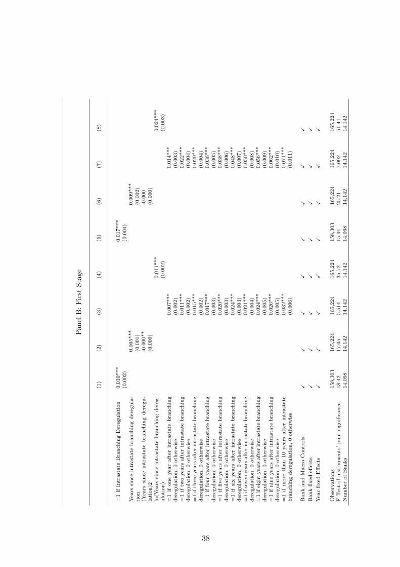
Panel

B:First

Stage

(1)

(2)

(3)

(4)

(5)

(6)

(7)

(8)

=1ifIntrastate

Branch

ingDereg

ulation

0.010***

0.017***

(0.002)

(0.004)

Yea

rssince

intrastate

branch

ingdereg

ula-

tion

0.005***

0.009***

(0.001)

(0.002)

(Yea

rssince

intrastate

branch

ing

dereg

u-

lation)2

-0.000**

-0.000

(0.000)

(0.000)

ln(Y

ears

since

intrastate

branch

ingdereg

-ulation)

0.011***

0.024***

(0.002)

(0.003)

=1

ifoneyea

rafter

intrastate

branch

ing

dereg

ulation,0oth

erwise

0.007***

0.014***

(0.002)

(0.003)

=1if

twoyea

rsafter

intrastate

branch

ing

dereg

ulation,0oth

erwise

0.011***

0.022***

(0.002)

(0.004)

=1ifth

reeyea

rsafter

intrastate

branch

ing

dereg

ulation,0oth

erwise

0.015***

0.029***

(0.002)

(0.004)

=1iffouryea

rsafter

intrastate

branch

ing

dereg

ulation,0oth

erwise

0.017***

0.036***

(0.003)

(0.005)

=1if

fiveyea

rsafter

intrastate

branch

ing

dereg

ulation,0oth

erwise

0.020***

0.038***

(0.003)

(0.006)

=1if

six

yea

rsafter

intrastate

branch

ing

dereg

ulation,0oth

erwise

0.024***

0.048***

(0.004)

(0.007)

=1ifseven

yea

rsafter

intrastate

branch

ing

dereg

ulation,0oth

erwise

0.021***

0.050***

(0.004)

(0.008)

=1ifeightyea

rsafter

intrastate

branch

ing

dereg

ulation,0oth

erwise

0.024***

0.056***

(0.005)

(0.009)

=1ifnineyea

rsafter

intrastate

branch

ing

dereg

ulation,0oth

erwise

0.026***

0.062***

(0.005)

(0.010)

=1if

more

than

10yea

rsafter

intrastate

branch

ingdereg

ulation,0oth

erwise

0.032***

0.071***

(0.006)

(0.011)

BankandMacroControls

XX

XX

XX

XX

Bankfixed

effects

XX

XX

XX

XX

Yea

rfixed

Effects

XX

XX

XX

XX

Observations

158,303

165,224

165,224

165,224

158,303

165,224

165,224

165,224

FTestofinstru

men

ts’jointsignifica

nce

18.42

17.05

5.514

35.72

15.91

25.21

7.092

51.41

Number

ofBanks

14,098

14,142

14,142

14,142

14,098

14,142

14,142

14,142

38

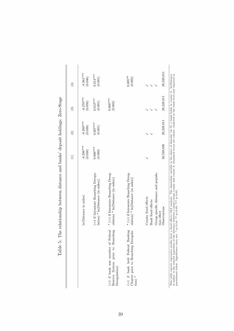
Tab

le5:

Therelationship

betweendistance

andbanks’

dep

ositholdings:Zero-Stage

(1)

(2)

(3)

(4)

ln(D

istance

inmiles)

-8.298***

-8.299***

-8.270***

-8.361***

(0.038)

(0.038)

(0.050)

(0.046)

(=1if

Intrastate

Branch

ingDereg

u-

lation)*ln(D

istance

(inmiles))

0.006***

0.007***

0.012***

0.014***

(0.000)

(0.001)

(0.001)

(0.001)

(=1

ifbank

wasmem

ber

ofFed

eral

Reserve

System

prior

toBranch

ing

Dereg

ulation)

*(=

1ifIntrastate

Branch

ingDereg

-ulation)*ln(D

istance

(inmiles))

0.000***

(0.002)

(=1

ifbank

held

Fed

eral

Banking

Charter

priorto

Branch

ingDereg

ula-

tion)*

*(=

1ifIntrastate

Branch

ingDereg

-ulation)*ln(D

istance

(inmiles))

0.005**

(0.002)

County

fixed

effects

XX

XX

Bankfixed

effects

XX

XGroupsp

ecificdistance

andpopula-

tioneff

ect

XX

Observations

30,528,636

28,228,011

28,228,011

28,228,011

This

table

reportsre

gre

ssion

resu

ltsfrom

afixed

effects

OLS

analysis.

The

dependentvariable

isth

esh

are

ofdeposits

(in

%)a

bank

hold

sin

county

A.’ln(D

ista

nce

inmiles)’is

thenatu

rallogarith

mofth

edista

ncebetw

een

abank’s

hom

ecounty

and

county

A.Sta

ndard

errors

are

robust,clu

stere

datth

ebank

leveland

reported

inpare

nth

ese

sbelow.Signifi

cancestars

are

:*

p<0.10,**

p<0.05,***

p<0.01.

39

Table 6: The impact of Diversification on Bank Risk - Instrumental Variables based on aBranching Deregulation-Gravity Model

Panel A: Second Stage

(1) (2) (3) (4)

Diversification Difference (HHI of deposits) -116.714***(21.518)

Diversification Difference (Number of Markets) -33.152***(4.395)

1 - Competitor’s Herfindahl Index of depositsacross counties

-189.206***(54.658)

1 - Herfindahl Index of deposits across counties72.854***(18.454)

ln(Number of competitor’s banking markets) -52.675***(17.403)

ln(Number banking markets) 28.908***(4.386)

Bank and Macro Controls X X X XBank fixed effects X X X XState-Year fixed Effects X X X X

Observations 185,518 185,518 185,518 185,518Number of Banks 10,070 10,070 10,070 10,070

Excluded Instrument:

Number of banking markets (predicted) X X

Herfindahl Index of assets across counties (predicted) X X

Variables in Zero Stage:

ln(Distance) X X X X

(Intrastate Branching Deregulation) * ln(Distance) X X X X

(=1 if bank holds national bank charter prior toBranching Deregulation prior to Branching Deregula-tion) * ln(Distance)

X X X X

This panel reports 2nd stage regression results from a bank and state-year fixed effects 2SLS analysis. The dependent variable is InverseZ-Score, defined as (Standard Deviation of ROA)/(ROA + Capital-Asset-Ratio)*1000. The endogenous variables are: ‘DiversificationDifference (HHI Deposits)/ Diversification Difference (Number of Markets)’, which is the relative difference between the a bank’s depositdispersion across markets/number of banking markets and its competitors; ‘1 - Herfindahl index of deposits across counties’, which isthe sum of squared deposit shares across counties for each bank, ‘1 - Competitor’s Herfindahl Index of deposits across counties’, whichis the bank’s competitors’ average concentration of deposits across counties; ‘ln(Number of banking markets)’, which is the naturallogarithm of the number of counties a bank has branches in; and ‘ln(Number of competitor’s banking markets)’, which is the naturallogarithm of a bank’s competitors’ average number of banking markets. The excluded instruments are from a gravity-deregulation model(see Table 5). Variables used in the gravity deregulation model are reported in the table. Standard errors are robust and reported inparentheses below. Significance stars are: * p<0.10, ** p<0.05, *** p<0.01.

40

A Data Appendix

1 Sample Construction

I compute Inverse Z-Score using semiannual information of profitability (Return on

Assets) obtained from ’Call Reports’. In particular, I compute a 5 period backward-

looking average of the standard deviation of Return on Assets, where the computa-

tion of standard deviation for period t uses information for periods t−4 to t. Because

of this, I am not able to compute it for the first four periods. I then merge this

information with ’Summary of Deposits’ data which are available on an annual basis

until 2006. This step limits the sample to annual bank observations for the years

1978 to 2006. Following previous research on intrastate branching deregulation, I

drop the states of Delaware and South Dakota from the sample since the structure

of the banking system in these two states was heavily affected by other laws, and

it is not possible to isolate the effect of intrastate branching deregulation. Inverse

Z-Score also exhibits very large volatility within the sample, and therefore I trim the

sample with respect to the 1st and 99th percentile of Inverse Z-Score. This eliminates

all outliers from the sample. In all regressions I restrict attention to banks that are

active in only one state and exist before and after intrastate branching deregulation.

Focusing on banks with branches in only one state allows me to better identify the

effect of intrastate branching deregulation on risk as these banks were restricted in

their geographic expansion.

2 Variable Definitions

Distress indicator I compute for each bank the annual change in its capital-asset

ratio, and construct an indicator variable that takes on the value of one if a bank’s

capital-asset ratio drops in two consecutive years by more than 1 percentage point

in each year.

41

CAMEL-ratings Laeven et al. (2002) find that a higher ratio of loan loss reserves

to capital, higher loan growth, lower net interest income to total income and lower

return on assets are significantly correlated with bank failure. Following Laeven

et al. (2002), I determine for each of these variables an indicator that takes on the

value of one if the variable for a given bank is worse than that of 75% of all the

sampled banks, and zero otherwise. For instance, if a bank’s return on asset is lower

than the 25th percentile, then this indicator is equal to one. Then, I sum these

indicator variables and construct ’CAMEL’-ratings for each bank and year taking

on values from 0 to 4, where higher values indicate higher failure risk.

3 Timing of Intrastate Branching Deregulation and Risk

The identification of the effect of intrastate branching deregulation on risk rests on

the assumption that the timing of deregulation is not affected by bank risk. This

implies that states did not deregulate because of a certain level of bank risk in a state.

To examine this graphically, I plot the year of intrastate branching deregulation

against (1) the median Inverse Z-Score and (2) the average change of median Inverse

Z-Score in each state, where I also condition on the aforementioned control variables.

Figures (Figure B.1(b)) and (Figure B.1(a)) are presented in the appendix and

suggest that there is no relationship between the timing of deregulation and the

level of bank risk in a state.

Kroszner and Strahan (1999) estimate an accelerated failure time model to iden-

tify forces of deregulation in each state. They measure the stability of a state’s

banking system by the share of assets held by failing banks and do not find evidence

that the level of bank (in)stability in a state is correlated with the timing of dereg-

ulation. I extend their methodology using my risk variables and test whether the

median Inverse Z-Score or the median annual change in Inverse Z-Score in a state

can predict the timing of deregulation (results available upon request).

42

1975

1980

1985

1990

1995

2000

Yea

r of

Intr

asta

te b

ranc

hing

der

egul

atio

n

−20 −10 0 10 20Median (Inverse Z−Score) before deregulation

(a) Level of Bank Risk

1975

1980

1985

1990

1995

2000

Yea

r of

Intr

asta

te b

ranc

hing

der

egul

atio

n

−1.5 −1 −.5 0 .5Median Change (Inverse Z−Score) before deregulation

(b) Change of Bank Risk

Figure A.I: Timing of Deregulation and Bank RiskNote: This figure plots the year of intrastate deregulation against the level/change of bank risk. Bank risk at thestate level is measured by the median Inverse Z-score in that state.

43

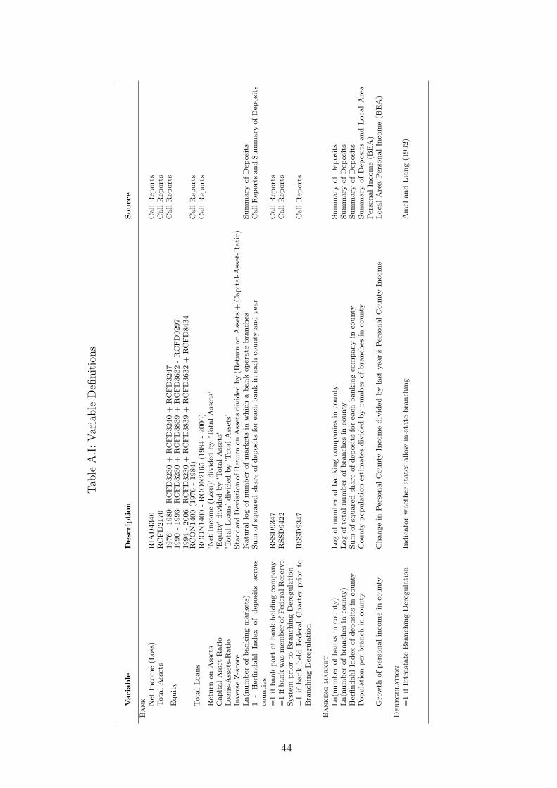
Tab

leA.I:Variable

Definitions

Variable

Desc

rip

tion

Source

Bank Net

Inco

me(L

oss)

RIA

D4340

CallRep

orts

TotalAssets

RCFD2170

CallRep

orts

Equity

1976-1989:RCFD3230+

RCFD3240+

RCFD3247

CallRep

orts

1990-1993:RCFD3230+

RCFD3839+

RCFD3632-RCFD0297

1994-2006:RCFD3230+

RCFD3839+

RCFD3632+

RCFD8434

TotalLoans

RCON1400(1976-1984)

CallRep

orts

RCON1400-RCON2165(1984-2006)

CallRep

orts

Return

onAssets

’Net

Inco

me(L

oss)’

divided

by’TotalAssets’

Capital-Asset-R

atio

’Equity’divided

by’TotalAssets’

Loans-Assets-Ratio

’TotalLoans’

divided

by’TotalAssets’

Inverse

Z-sco

reStandard

Dev

iationofReturn

onAssetsdivided

by(R

eturn

onAssets+

Capital-Asset-R

atio)

Ln(number

ofbankingmarkets)

Natu

rallogofnumber

ofmarketsin

whichabankoperate

branch

esSummary

ofDep

osits

1-HerfindahlIndex

ofdep

osits

across

counties

Sum

ofsquaredsh

are

ofdep

osits

forea

chbankin

each

county

andyea

rCallRep

ortsandSummary

ofDep

osits

=1ifbankpart

ofbankholdingco

mpany

RSSD9347

CallRep

orts

=1ifbankwasmem

ber

ofFed

eralReserve

System

priorto

Branch

ingDereg

ulation

RSSD9422

CallRep

orts

=1if

bank

held

Fed

eralCharter

priorto

Branch

ingDereg

ulation

RSSD9347

CallRep

orts

Banking

market

Ln(number

ofbanksin

county)

Logofnumber

ofbankingco

mpaniesin

county

Summary

ofDep

osits

Ln(number

ofbranch

esin

county)

Logoftotalnumber

ofbranch

esin

county

Summary

ofDep

osits

HerfindahlIndex

ofdep

osits

inco

unty

Sum

ofsquaredsh

are

ofdep

osits

forea

chbankingco

mpanyin

county

Summary

ofDep

osits

Populationper

branch

inco

unty

County

populationestimatesdivided

bynumber

ofbranch

esin

county

Summary

ofDep

osits

andLoca

lArea

PersonalInco

me(B

EA)

Growth

ofpersonalinco

mein

county

Changein

PersonalCounty

Inco

medivided

bylast

yea

r’sPersonalCounty

Inco

me

Loca

lAreaPersonalInco

me(B

EA)

Deregulation

=1ifIntrastate

Branch

ingDereg

ulation

Indicatorwhether

statesallow

in-state

branch

ing

Amel

andLiang(1992)

44

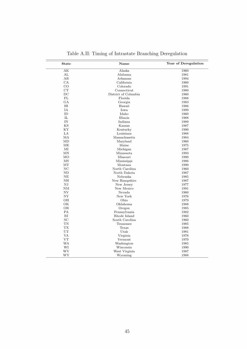
Table A.II: Timing of Intrastate Branching Deregulation

State Name Year of Deregulation

AK Alaska 1960AL Alabama 1981AR Arkansas 1994CA California 1960CO Colorado 1991CT Connecticut 1980DC District of Columbia 1960FL Florida 1988GA Georgia 1983HI Hawaii 1986IA Iowa 1999ID Idaho 1960IL Illinois 1988IN Indiana 1989KS Kansas 1987KY Kentucky 1990LA Louisiana 1988MA Massachusetts 1984MD Maryland 1960ME Maine 1975MI Michigan 1987MN Minnesota 1993MO Missouri 1990MS Mississippi 1986MT Montana 1990NC North Carolina 1960ND North Dakota 1987NE Nebraska 1985NH New Hampshire 1987NJ New Jersey 1977NM New Mexico 1991NV Nevada 1960NY New York 1976OH Ohio 1979OK Oklahoma 1988OR Oregon 1985PA Pennsylvania 1982RI Rhode Island 1960SC South Carolina 1960TN Tennessee 1985TX Texas 1988UT Utah 1981VA Virginia 1978VT Vermont 1970WA Washington 1985WI Wisconsin 1990WV West Virginia 1987WY Wyoming 1988

45