Finance and Economics Discussion SeriesDivisions of Research & Statistics and Monetary Affairs

Federal Reserve Board, Washington, D.C.

Bank Core Deposits and the Mitigation of Monetary Policy

Lamont Black, Diana Hancock, and Wayne Passmore

2007-65

NOTE: Staff working papers in the Finance and Economics Discussion Series (FEDS) are preliminarymaterials circulated to stimulate discussion and critical comment. The analysis and conclusions set forthare those of the authors and do not indicate concurrence by other members of the research staff or theBoard of Governors. References in publications to the Finance and Economics Discussion Series (other thanacknowledgement) should be cleared with the author(s) to protect the tentative character of these papers.

10/5/2007

BANK CORE DEPOSITS AND THE MITIGATION OF MONETARY POLICYϒ

Lamont Black, Diana Hancock and Wayne Passmore Board of Governors of the Federal Reserve System

Washington, DC 20551

ABSTRACT

We consider the business strategy of some banks that provide relationship loans (where they have loan origination and monitoring advantages relative to capital markets) with core deposit funding (where they can pass along the benefit of a sticky price on deposits). These “traditional banks” tend to lend out less than the deposits they take in, so they have a “buffer stock” of core deposits. This buffer stock of core deposits can be used to mitigate the full effect of tighter monetary policy on their bank-dependent borrowers. In this manner, the business strategy of “traditional banks” acts as a “core deposit mitigation channel” to provide funds to bank-dependent borrowers when there are monetary shocks. In effect, there is no bank lending channel of monetary policy associated with these traditional banks.

In contrast, other banks mainly rely on managed liabilities that are priced at market rates. These banks do not have to shift from insured deposits to managed liabilities in response to tighter monetary policy. At the margin, their loans are already funded with managed liabilities. For these banks as well, there is no unique bank lending channel of monetary policy.

The only banks that are likely to raise loan rates substantially in response to an increase in the federal funds rate are banks with a high proportion of relationship loans that are close to a loan-to-core deposit ratio of one. These banks must substitute higher cost nondeposit liabilities, which have an external finance premium, for core deposits, which do not because of deposit insurance. Some of these banks may also face higher marginal costs as their loan-to-core deposit ratio approaches one because of the costs associated with lending to default-prone relationship borrowers. It is among these banks (which we refer to as high relationship lenders), and only these banks, that we find evidence of a bank lending channel – they significantly reduce lending in response to a monetary contraction. Importantly, these banks hold only a small fraction of U.S. banking assets. Thus, in the United States, the bank lending channel seems limited in scope and importance, mainly because so few banks that specialize in relationship lending switch from core deposits to managed liabilities in response to changes in interest rates. ϒ The views expressed are those of the authors and do not necessarily reflect those of the Board of Governors of the Federal Reserve System or its staff. The authors wish to thank Jerry Dwyer and participants at the conference on “The Credit Channel of Monetary Policy in the 21st Century” (held at the Federal Reserve Bank of Atlanta on June 14, 2007) for their useful comments. The authors thank Reid Dorsey-Palmateer and Jessica Lee for their outstanding research assistance. All errors remain those of the authors.

10/5/2007

- 1 -

I. INTRODUCTION There is considerable interest in whether monetary policy can influence the

supply of intermediated credit, particularly the loans made by commercial banks to bank-

dependent borrowers (e.g., small and medium-sized businesses) who may not be able to

obtain credit elsewhere. Much of the discussion of the “bank lending channel” has

focused on whether monetary policy can significantly affect the relative pricing of bank

loans by reducing bank’s access to loanable funds (e.g., Bernanke and Gertler, 1995).

This effect of monetary policy, transmitted through the level and composition of bank

assets, would be in addition to the traditional money supply and interest-rate effects,

which may also be reflected in declining bank liabilities.

The transmission mechanism for the bank lending channel is easily explained, but

has proved difficult to empirically detect. During a monetary tightening, open-market

sales by the Fed would likely shrink banks’ core deposit base and force these depositories

to rely more heavily on managed liabilities. As these depositories shift their liabilities

toward managed liabilities, the relative cost of their funds increases.

The shift by banks from insured retail deposits to nondeposit (or managed)

liabilities creates an external finance premium for banks, similar to the external finance

premium of firms that underlies financial accelerator models. The people and institutions

that lend money to banks without the backing of the government (nondeposit liabilities)

charge banks a credit premium based on the bank’s credit quality. Banks respond by

raising loan rates, which increases the cost of financing for bank-dependent borrowers,

and possibly reduces the supply of loans to such borrowers.

Although the data on interest rate spreads (for banks’ cost of funds and for the

prime loans offered by banks), as well as on the terms of small business lending, are

consistent with the bank lending channel mechanism, such data are also consistent with a

tightening of monetary policy that worsens both borrowers’ and banks’ balance sheets.

Such balance sheet effects alone could conceivably explain why it is observed that

borrowing becomes more expensive (i.e., there are higher spreads) and more difficult

(i.e., there are tougher terms for bank lending) during periods of tighter monetary policy.

Thus, the identification of a “pure” bank lending channel where the contraction of loans

10/5/2007

- 2 -

reflects rising funding costs for banks, and not borrower balance sheet deterioration, has

been difficult.

Because it has been difficult to detect the bank lending channel using aggregate

data, some researchers have considered how monetary policy differentially impacts the

lending behavior of a cross-section of individual banks. For example, Kashyap and Stein

(1995 and 2000), have argued that small banks have the most costly access to external

funds, and that among small banks, those with less liquid portfolios (i.e., those with a

smaller buffer stock of securities) would be most likely to raise their loan rates. If these

banks increase their rates more than other banks when monetary policy causes interest

rates to increase, then their contraction in loans should be more pronounced than the

contraction in loans at other banks. Empirically, one should observe smaller banks with

less access to wholesale sources of funds and with smaller securities portfolios to have a

greater response to monetary contractions. (This identification strategy assumes that

there is little correlation between the securities holdings of small banks and the

propensity of their borrowers to contract their demand for loans.)

The empirical evidence during the 1980’s and early 1990’s is consistent with this

view, with tighter monetary policy resulting in a larger contraction in lending at smaller

banks with the least liquid balance sheets. Not surprisingly, for the largest banks, the

liquidity of the balance sheet is less important because such banks have an easier time

accessing managed liability markets.

However, during the past decade, the liquidity at small banks has noticeably

improved. Smaller institutions have a much wider variety of low-cost alternatives to

deposits, such as Federal Home Loan Banks advances and brokered insured CDs.

Furthermore, securitization opportunities are available to all banks now, including the

smallest. Finally as we suggest here, some banks may be aware that their borrowers are

more sensitive to increases in the loan rate, and thus might seek to adjust their balance

sheets to immunize their bank-dependent borrowers from interest rate changes.

Consequently, we propose a different approach to identification of the bank lending

channel.

In this paper, we consider the business strategy of some banks that provide

relationship loans (where they have loan origination and monitoring advantages relative

10/5/2007

- 3 -

to capital markets) with core deposit funding (where they can pass along the benefit of a

sticky price on deposits). These “traditional banks” tend to lend out less than the deposits

they take in, so they have a “buffer stock” of core deposits. This buffer stock of core

deposits can be used to mitigate the full effect of tighter monetary policy on their bank-

dependent borrowers. In this manner, the business strategy of “traditional banks” acts as a

“core deposit mitigation channel” to provide funds to bank-dependent borrowers when

there are monetary shocks. In effect, there is no bank lending channel of monetary policy

associated with these traditional banks.

In contrast, other banks mainly rely on managed liabilities that are priced at

market rates. These banks do not have to shift from insured deposits to managed

liabilities in response to tighter monetary policy. At the margin, their loans are already

funded with managed liabilities. For these banks as well, there is no unique bank lending

channel of monetary policy.

The only banks that are likely to raise loan rates substantially in response to an

increase in the federal funds rate are banks with a high proportion of relationship loans

that are close to a loan-to-core deposit ratio of one. These banks must substitute higher

cost nondeposit liabilities, which have an external finance premium, for core deposits,

which do not because of deposit insurance. Some of these banks may also face higher

marginal costs as their loan-to-core deposit ratio approaches one because of the costs

associated with lending to default-prone relationship borrowers.

Thus, our theory suggests that banks with a relatively high proportion of

relationship borrowers should have lower loan-to-deposit ratios. Moreover, such banks

should increase loan rates more in response to higher market rates when they become

close to their core lending capacity. (We define their core lending capacity as the dollar

amount of loans that can be funded with core deposits.) Our empirical approach is to

estimate a model similar to the one estimated in Kashyap and Stein (2000), but we exploit

interaction terms between loan-to-core deposit ratios and the federal funds rate (as a

measure of monetary policy).

Our empirical findings are consistent with our theory. We find evidence of a

bank lending channel for monetary policy only for banks that specialize in relationship

lending and also have a loan-to-core deposit ratio near one – these banks significantly

10/5/2007

- 4 -

reduce lending in response to a monetary contraction. For all other banks, there is no

evidence of a bank lending channel.

The remainder of our paper is organized as follows: Section II provides some

background on our view of banking. Section III is a description of our strategy to

identify a bank lending channel, including a graphical description of the underlying

theory. This section provides the intuition behind our empirical approach. Section IV

provides the theory more formally. Section V describes our empirical approach, including

the data needed to implement it, and discusses our findings. Section VI extends our

analysis to cover some recent themes concerning the bank lending channel, and Section

VII concludes with a brief discussion of the implications of our findings.

II. THE UNIQUE BUSINESS OF BANKING

In this paper, we argue that some banks are special because they have access to

deposits with sticky interest rates -- core deposits – and because they focus on

relationship or “bank-dependent” borrowers. In our theory, these two business functions

are intertwined. Core deposits permit banks to make implicit contractual agreements with

bank-dependent borrowers that would be infeasible if they had to pay market-sensitive

rates for such funds.1 Traditionally, the transmission mechanism for the bank lending

channel has focused on core deposits being a relatively low-cost form of bank funding

which is not perfectly substitutable with managed liabilities. Here, we change the

emphasis to highlight the fact that many banks aggressively pursue core deposits as a

distinct and profitable line of business. The availability of core deposits creates the

opportunity for banks to mitigate the effects of interest rate shocks on their bank-

dependent borrowers.

Indeed, empirical evidence suggests that banks funded more heavily with core

deposits provide more loan rate smoothing in response to exogenous changes in credit

risk (Berlin and Mester, 1999). Moreover, access to core deposits may allow banks to

negotiate multi-period state-contingent contracts that are more efficient than single-

period or multi-period fixed-payoff contracts. For example, banks with greater market

1 Price rigidity in the U.S. market for consumer bank deposits is well established. See, for example, Hannan and Berger (1991), Neumark and Sharp (1992), and Kahn, Pennacchi, and Sopranzetti (1999).

10/5/2007

- 5 -

power in their core deposit market(s) may be better positioned to gain an implicit equity

interest in new firms (because of a higher probability of lending to successful

entrepreneurs in the future) owing to their more stable cost of funds (Petersen and Rajan,

1995). In addition, banks are liquidity providers to their loan commitment customers and

to their transactions account depositors. In this dual liquidity provision role, banks

typically face increased take-down demands from borrowers constrained by tight market

conditions at the same time that they experience deposit inflows (Gatev and Strahan,

2005). This synergy allows banks to hold less liquid assets to fulfill liquidity needs

(Kashyap, Rajan, and Stein, 2002). In effect, banks can insure bank-dependent borrowers

against systematic declines in liquidity at a lower cost than can other financial

institutions.

This is not to say that changes in the cost of managed liabilities are irrelevant.

Innovations, such as loan securitization methods, have increasingly enabled banks to

provide loans that are funded with managed liabilities at market-based rates to some

customers (i.e., those who typically have more collateral or net worth than is held by

bank-dependent borrowers). For example, the loan pricing on most conventional, fixed-

rate, 30-year home mortgages is determined in the national market because such loans are

frequently sold to securitizers, such as Fannie Mae and Freddie Mac. Similarly, most

credit card loan rates are heavily influenced by secondary markets because most such

loans are now securitized using asset-backed securities. Such customers, however, are

arguably not bank-dependent, and therefore, would not be unduly influenced by the bank

lending channel described above.

We posit that some banks may have a business strategy to provide relationship

loans (where they have loan origination and monitoring advantages relative to capital

markets) with core deposit funding (where they can pass along the benefit of a sticky

price on deposits). These “traditional banks” might invest in excess core lending capacity

and thereby circumvent the full effect of tighter monetary policy on their bank-dependent

borrowers. In contrast, banks that rely mainly on managed liabilities that are priced at

market rates would need to raise lending rates, or tighten lending standards, in response

to tighter monetary policy.

10/5/2007

- 6 -

III. IDENTIFICATION OF A BANK LENDING CHANNEL

As argued by Kashyap and Stein (1995), a measure of the bank lending channel is

how the spread between the bank lending rate and the risk free rate changes in response

to a rise in short-term interest rates. If the loan rate increases one-for-one (that is, the

spread remains constant), then there is no bank lending channel.

We modify this approach to account for loan default. Clearly, if a borrower can

default, then an increase in risk-free interest rates might be associated with an increase in

lending rates that exceeds the increase in the risk-free rate. For example, in the balance

sheet channel described above, an increase in the market rates causes the value of the

borrower collateral to fall and, perhaps, their cash flows to diminish. In response to this

deterioration in credit quality, the bank would raise rates more than one-for-one in

response to an increase in the risk-free rate. In such circumstances, bank loan rates can

rise more than the risk free rate, yet this increase may not be evidence of a pure bank

lending channel.

Some bank borrowers might be affected more by an increase in the bank’s loan

rates than others, and this additional effect might be associated with the unique

characteristics of bank lending. We define “relationship borrowers” as borrowers with

three characteristics. First, their probability of success is more highly influenced by the

bank’s loan rate than the probability of success for other borrowers. A higher loan rate

noticeably raises their odds of default. Second, relationship borrowers are more costly

for these banks because of the interest rate smoothing described above and because these

borrowers require more services than other borrowers. Third, relationship borrowers are

more likely to engage in opaque activities, which give them a higher external finance

premium (making them more reliant on bank loans for financing).2 This higher external

finance premium also may imply a higher deadweight loss should they default.

Our identification strategy is in the spirit of Kashyap and Stein (2000), who

compare the differences in responses to monetary policy between large and small banks,

and then look at the differences within each group. As we will show formally in the next

section, the characteristics of relationship borrowers create sharply different responses to

2 As a result, banks that fund mainly relationship borrowers may be themselves more opaque, raising the banks’ external finance premium as well.

10/5/2007

- 7 -

interest rate shocks by banks with large proportions of relationship borrowers when

compared to those of banks with low proportions of relationship borrowers. We then

compare within each group their response to monetary shocks given their loan-to-core

deposit ratios, which are related to the costs of the relationship lending. The Kashyap

and Stein (2000) difference-in-difference identification strategy argues that evidence of a

bank lending channel can be found by examining how small banks differ in response to

monetary shocks based on different holdings of securities holdings. In contrast, our

approach argues that evidence of a bank channel can be found by examining how banks

with many relationship borrowers differ in response to monetary shocks based on

different loan-to-core deposit ratios.

As shown in figure 1, the loan supply functions for high relationship lenders and

low relationship lenders are strikingly different. Banks with larger proportions of

relationship borrowers – high relationship lenders – charge higher loan rates to cover

their borrowers’ higher expected default rates and higher relationship costs. However, to

the degree that such banks have low loan-to-core deposit ratios, these higher rates can be

substantially mitigated. At the lowest loan-to-core deposit ratios, there are fewer loans

that incur relationship costs and there is greater capacity to provide lower-cost

relationship lending services. As loan-to-core deposit ratios rise, the loan rates change a

little for the low relationship lenders (i.e., the banks with a small proportion of

relationship borrowers). But for relationship borrowers at high relationship lenders, rates

rise quickly because the default rates for these borrowers rise and, at the same, the costs

of maintaining the relationships increase.

The response of each relationship lender group to an interest rate shock is shown

in figure 2. The low relationship lender group has a smaller response. (The vertical axis

describes the multiple of the loan rate relative to the change in the risk free rate. For

example, 1.2 means that a 100 basis point increase in the risk free rate increases the loan

rate 120 basis points.) At relatively low loan-to-core deposit ratios, both groups show

little change in their response to interest rate shocks because deposit funding is readily

available for all borrowers (securities holdings are simply decreased to free up the

deposits for funding loans). Similarly, at relatively high loan-to-core deposit ratios (those

greater than one), high cost market-based funds (nondeposit liabilities) are readily

10/5/2007

- 8 -

available for both high and low relationship lender groups and thus their response to

interest rate shocks is unchanging as the loan-to-core deposit ratio increases.

Only when the loan-to-core deposit ratio is close to one does a notable difference

in response appear between the groups. (Recall, core deposits here are a short-hand for

bank liabilities whose rates embed a minimal external finance premium, such as insured

deposits and Federal Home Loan Bank advances.) As loans approach core lending

capacity, the odds of default for relationship borrowers rise at the same time that the

bank’s costs of supporting these relationships increase. These effects interact to push the

bank to raise its loan rates all the more as market rates rise. Close to this barrier, the high

relationship lenders show an upward tilt in how much they increase loan rates in response

to an interest rate shock.

Thus, our theory makes the following predictions:

1. High relationship lenders will have lower loan-to-core deposit ratios than low

relationship lenders. (Because lending to relationship borrowers imposes higher

market premiums on these banks if they need to switch to nondeposit funding

sources.)

2. High relationship lenders who are close to exhausting their capacity to fund loans

with deposits will raise loan rates more sharply in response to changes in market

interest rates. Thus, their lending should fall more in response to a monetary

contraction than other banks. This is a pure bank lending channel effect.3

3. All banks—both high and low relationship lenders— that have substantial excess

core lending capacity should not vary how they change loan rates in response to a

change in market rates. Their costs of funds is not varying in response to market

rates; their main cost of higher market rates is the opportunity costs associated

with holding fewer securities and the possible deterioration of their borrower’s

balance sheets. Consequently, it is difficult to identify the pure bank lending

channel effects among these lenders.

3 Note that this result is similar to the Kashyap and Stein (1995) bank lending channel effect. High intensity relationship lenders are usually smaller banks and those with high loan-to-core deposit ratios also have low securities-to-asset ratios. Thus, our model and its predictions provide a different interpretation of the Kashyap and Stein (2000) result.

10/5/2007

- 9 -

4. All banks—both high and low relationship lenders— that have exhausted their

core lending capacity for funding loans should not vary how they change loan

rates in response to a change in market rates. For these banks, their marginal

funding is already determined in the market and these banks simply pass-through

market rate increases. It seems unlikely that a pure bank lending channel exists

among these lenders.

IV. A SIMPLE THEORY OF RELATIONSHIP BORROWING AND CORE DEPOSITS

We posit that the business of banking is providing core deposits and using those

deposits to fund “relationship borrowers.” Core deposits are by definition less sensitive

to fluctuations in market interest rates (because of deposit insurance) and they have little

external finance premium embedded within their costs. Banks have a choice between

funding loans using managed liabilities, which are priced at market rates, and funding

loans using core deposits. Banks can always raise funds at market rates. Moreover, there

is no constraint on banks to substitute market-based funds for core deposits. In a

nutshell, we argue that a bank has the capacity and the willingness to fund a relationship

borrower under all circumstances, but it is more profitable to fund these loans with core

deposits.

LOAN SUPPLY

The borrower has an exogenous constraint on the amount borrowed, denoted *L .

The loan is invested in a project that returns Lα , where *L is the amount borrowed. The

project pays ( )Lr Lα − , where Lr L is both the interest and principal of the loan. If the

project succeeds ( )Lrα − is positive. If the project fails, it is negative and the borrower

walks away. The probability q that the project pays off is:

( )Lr

q f dα α∞

= ∫ (1)

Banks are unique from other financial institutions when they are in the business of

“farming” core deposits. This process involves building bank branches, ATMs and

10/5/2007

- 10 -

other methods of handling retail transaction accounts and finding consumers who value

convenience and who are generally not sensitive (with their money placed in these

accounts) to changes in interest rates. As a result, core deposits rates are relatively low

cost and are very sticky in response to increases in market rates.

Banks also fund relationship borrowers. Banks overcome adverse selection

problems by investing in a relationship with the borrower and through this process come

to know the true default probability for the firm. Moreover, banks smooth interest rate

fluctuations for these borrowers because they know changes in loan rates can

dramatically influence the odds of success for these borrowers. Such loan rate smoothing

can cost the bank money, but this cost is mitigated the more the bank relies on core

deposits. If loans are a small portion of core deposits, the marginal increase in the cost of

funds is almost zero.

In this business, bank profits depend on core deposit capacity. To collect a given

amount of deposits, banks must raise and invest capital, K , by paying the market return

on equity, er . After making this investment, deposits cost the bank d er r< , where we

assume, for convenience, that dr is not influenced in the short-run by fluctuations in

market interest rates. Brick and mortar investments place a capacity constraint, D , on

the amount of the core deposits that are collected, D , and therefore on the amount of

loans that can be funded by core deposits.

Bank profits depend on whether core lending capacity is adequate (that is,

whether there are sufficient core deposits to fund the loan portfolio). In a “low demand”

environment, banks can retain all the loans they originate. Excess core deposits are

invested in market-rate securities where the return is less than the return on loans, or

L altr r> . If the return to the firm’s project exceeds the firm’s obligation to the bank

( 0)Lrα − ≥ , then the bank receives its promised repayment. If the return to the firm’s

project falls short, the bank receives the liquidation value of the project, δ .

When loan demand is low relative to core deposits ( )LD L> , a bank’s expected

profit on a loan is:

2

2(1 ) ( ) ,

2 2d

L low low alt low erLqr L q L r D L L r K D

Dρπ δ ⎛ ⎞= + − + − − − −⎜ ⎟⎝ ⎠

(2)

10/5/2007

- 11 -

where δ is the return given the firm defaults and ρ is the cost of smoothing loan rates,

which rises as the dollar value of the loans extended rises and falls as core deposits

increase. The costs of smoothing will be lower, or higher, depending on whether loans

are above, or below, the bank’s deposit capacity, D .

A bank maximizes profits with respect to the dollar amount of loans extended,

which in the low-demand case leads to the first-order condition where the loan rate is:

23 (1 )2alt

L

Lr qDrq

ρ δ⎛ ⎞+ − −⎜ ⎟⎝ ⎠= (3)

UNDERSTANDING THE BANK LENDING CHANNEL

In equilibrium, loan supply equals loan demand. Loan demand is a function of

the interest rate and the payoff from the firm’s investments:

,( )S Dlow low LL L r α= .

The equilibrium rate, which is rate observed for the loans on the bank’s balance sheet, is:

2

,( )3 (1 )2

.

Dlow L

alt

L

L r qr q

Dr

q

ρ δ⎛ ⎞

+ − −⎜ ⎟⎝ ⎠= (4)

Note that if loan payment is certain ( 1)q = , then the loan rate is the same as the market

rate (and because there is no motivation for loan smoothing, 0ρ = ). In this case, there

is no bank lending channel, and the loan rate equals the market rate.

The bank lending channel describes how the interest rate on loans changes in

response to an increase in market interest rates (created by the Federal Reserve or other

exogenous events). Taking the total derivative of equation (4) with respect to altr and

rearranging terms yields

10/5/2007

- 12 -

2

,

1 .( )3

23

L

Dalt low altaltD

Low

L L

rr L r q

rDLL qq

r r qD D

ρ δρ

∂=

∂ ⎡ ⎤⎛ ⎞⎢ ⎥+ −⎜ ⎟⎢ ⎥∂ ∂⎛ ⎞ ⎝ ⎠− +⎜ ⎟ ⎢ ⎥∂ ∂⎝ ⎠ ⎢ ⎥⎢ ⎥⎣ ⎦

(5)

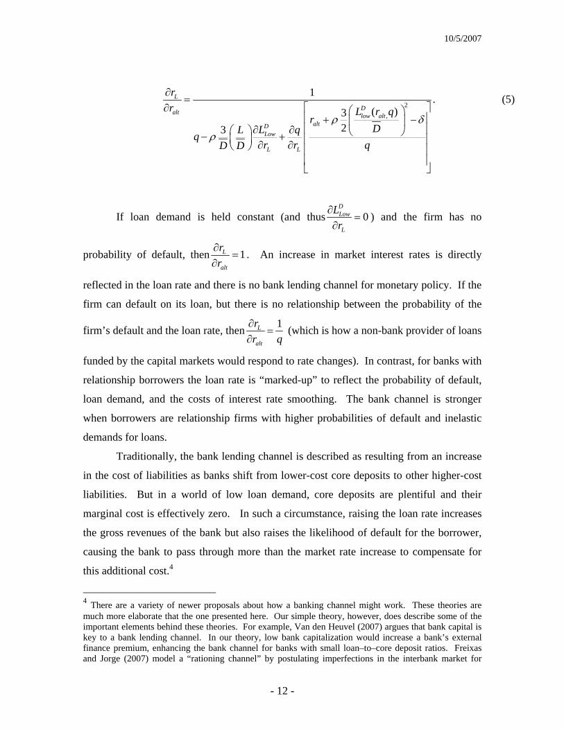
If loan demand is held constant (and thus 0DLow

L

Lr

∂=

∂) and the firm has no

probability of default, then 1L

alt

rr∂

=∂

. An increase in market interest rates is directly

reflected in the loan rate and there is no bank lending channel for monetary policy. If the

firm can default on its loan, but there is no relationship between the probability of the

firm’s default and the loan rate, then 1L

alt

rr q∂

=∂

(which is how a non-bank provider of loans

funded by the capital markets would respond to rate changes). In contrast, for banks with

relationship borrowers the loan rate is “marked-up” to reflect the probability of default,

loan demand, and the costs of interest rate smoothing. The bank channel is stronger

when borrowers are relationship firms with higher probabilities of default and inelastic

demands for loans.

Traditionally, the bank lending channel is described as resulting from an increase

in the cost of liabilities as banks shift from lower-cost core deposits to other higher-cost

liabilities. But in a world of low loan demand, core deposits are plentiful and their

marginal cost is effectively zero. In such a circumstance, raising the loan rate increases

the gross revenues of the bank but also raises the likelihood of default for the borrower,

causing the bank to pass through more than the market rate increase to compensate for

this additional cost.4

4 There are a variety of newer proposals about how a banking channel might work. These theories are much more elaborate that the one presented here. Our simple theory, however, does describe some of the important elements behind these theories. For example, Van den Heuvel (2007) argues that bank capital is key to a bank lending channel. In our theory, low bank capitalization would increase a bank’s external finance premium, enhancing the bank channel for banks with small loan–to–core deposit ratios. Freixas and Jorge (2007) model a “rationing channel” by postulating imperfections in the interbank market for

10/5/2007

- 13 -

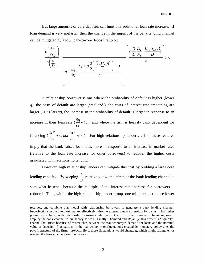
But large amounts of core deposits can limit this additional loan rate increase. If

loan demand is very inelastic, then the change in the impact of the bank lending channel

can be mitigated by a low loan-to-core deposit ratio or:

,

22

,

( )31 0.

( )32

Dlow altL

Lalt

Dlow alt

alt

L

L r qqrrD Dr

L qL r qrD

Dqqr q

ρ

ρ δ

⎡ ⎤⎡ ⎤⎛ ⎞ ∂∂∂ ⎢ ⎥⎢ ⎥⎜ ⎟ ∂∂ − ⎢ ⎥⎝ ⎠ ⎣ ⎦= >⎢ ⎥⎛ ⎞ ⎡ ⎤⎡ ⎤∂ ⎛ ⎞ ⎢ ⎥⎜ ⎟ ⎢ ⎥⎢ ⎥+ −⎝ ⎠ ⎜ ⎟ ⎢ ⎥⎣ ⎦⎢ ⎥⎢ ⎥∂ ⎝ ⎠+⎢ ⎥⎢ ⎥∂⎢ ⎥⎢ ⎥

⎢ ⎥⎢ ⎥⎣ ⎦⎣ ⎦

A relationship borrower is one where the probability of default is higher (lower

q), the costs of default are larger (smallerδ ), the costs of interest rate smoothing are

larger ( ρ is larger), the increase in the probability of default is larger in response to an

increase in their loan rate ( 0qr∂∂

), and where the firm is heavily bank dependent for

financing ( 0, 0D D

L L

L Lnotr r

∂ ∂≈

∂ ∂). For high relationship lenders, all of these features

imply that the bank raises loan rates more in response to an increase in market rates

(relative to the loan rate increase for other borrowers) to recover the higher costs

associated with relationship lending.

However, high relationship lenders can mitigate this cost by building a large core

lending capacity. By keeping LD

relatively low, the effect of the bank lending channel is

somewhat lessened because the multiple of the interest rate increase for borrowers is

reduced. Thus, within the high relationship lender group, one might expect to see lower

reserves, and combine this model with relationship borrowers to generate a bank lending channel. Imperfections in the interbank market effectively raise the external finance premium for banks. This higher premium combined with relationship borrowers who can not shift to other sources of financing would amplify the bank channel in our theory as well. Finally, Diamond and Rajan (2006) present a “liquidity” channel that arises because of mismatches between the real economy’s demand for loans and the nominal value of deposits. Fluctuations in the real economy or fluctuations created by monetary policy alter the payoff structure of the firms’ projects. Here, these fluctuations would change q, which might strengthen or weaken the bank channel described above.

10/5/2007

- 14 -

loan-to-core deposit ratios and a more pronounced increase in the drop in loan supply that

occurs in response to an interest rate increase (as the loan-to-core deposit ratio increases).

HIGH LOAN DEMAND

In the case of high loan demand ( )LD L< , the bank must turn to market-based

funding (that is, nondeposit liabilities) to lend at the margin. It cannot rely exclusively on

its core deposits. Market-based funds are provided to bank j at a rate alt jr φ+ , where jφ

is a market premium that reflects the risks associated with lending to the bank. It seems

reasonable that a bank that is more focused on relationship borrowers (a high relationship

lender) might have a higher credit risk premium embedded in its nondeposit lending (a

higherφ ).

With high loan demand, a bank’s expected profits on a loan is:

2

*(1 ) ( )( ) ,2 2

D dL High High alt j High e

rpqr L q L r L D D r K Dπ δ φ= + − − + − − − − (6)

which implies that the yield on a bank’s loans is:

(1 )

.alt jL

r qr

qφ δ+ − −

= (7)

In this case, the change in loan rates with respect to market rates is:

1 ,L

alt jalt

L

rrr qq

r qφ δ

∂=

+ −∂ ⎡ ⎤∂+ ⎢ ⎥∂ ⎣ ⎦

(8)

which is positive.

LOAN SUPPLY AND LONG-RUN CORE LENDING CAPACITY

Core lending capacity is fixed in the short-run. Loan smoothing costs are linked

to deposits because deposits have almost no marginal costs. In the long-run, the bank

would like its loan-to-core deposit ratio to be as small as possible (that is, it wants a big

core lending capacity) so long as the marginal profitability of additional core lending

capacity does not exceed the marginal costs of using market-based funds. Thus, long-run

core lending capacity is:

10/5/2007

- 15 -

2alt j

d

rD

r

ρφ+ −= (9)

At the margin, a bank compares the costs associated with relationship borrowers

to the external financing costs (including the external finance premium) associated with

nondeposit funding. If the external finance premium is high and the costs associated with

relationship borrowers are low, the bank will desire a larger deposit capacity relative to

loans (that is, a smaller LD

). Thus, high relationship lenders typically desire smaller

loan-to-core deposit ratios, and low relationship lenders typically would prefer bigger

loan-to-core deposit ratios.

V. OUR EMPIRICAL APPROACH

DATA. This section describes the data sources and the data elements that were

constructed to estimate our empirical model and to stratify banking organizations into

different relationship lending groups. We describe (1) the balance sheet data for

individual banks, (2) the reasons for and methods used to aggregate such information for

entities that are subsidiaries within a bank holding company, (3) the factors used to

control for regional and macroeconomic conditions, and (4) the data used for the

stratification strategy that is implemented prior to the estimation of the empirical model.

Then, we take a brief look at the stratified data across time before discussing the

specification of the model that was estimated.

BANK BALANCE SHEET INFORMATION. We used Call Reports for individual,

federally-insured, domestically chartered commercial banks to construct quarterly data

for eight bank balance sheet variables consisting of four lending activity measures –

commercial and industrial loans (C&I), relationship-based business loans (RBL),

residential mortgages (MORT), and total loans (LOANS) – securities (SEC), core

deposits (DEP), equity capital (K), and total assets (A). These data were constructed for

the period 1991:Q4 – 2005:Q4, inclusive, since the data used to create RBL are not

available prior to 1993:Q2.5

5 Because RBL is only used to stratify banks, we were able to take other data back earlier to use as lags in the empirical model.

10/5/2007

- 16 -

The two business lending categories, C&I and RBL, each include only loans to

businesses domiciled in the United States. C&I is the amount outstanding of all such

business loans, regardless of their original amount.6 In contrast, RBL is defined to be

business loans with original amounts of $1 million or less.7

Residential mortgages (MORT) include (1) the amount outstanding of all

permanent loans secured by 1-to-4 family residential properties, and (2) the amount

outstanding of loans extended under revolving, open-end lines of credit secured by 1-4

family residential properties. 8 Such open-end lines of credit, commonly referred to as

“home equity lines,” are typically secured by a junior lien and are usually accessible by

check or credit card.9 As with C&I loans, we included only domestic mortgage loans in

our measure of mortgage lending.

In contrast, total loans (LOANS) are measured on a consolidated basis (i.e., both

domestic and foreign loans are included). This comprehensive lending measure equals

the aggregate book value of all loans made by the bank (before the deduction of valuation

reserves).10

Securities (SEC) are also measured on a consolidated basis, since either domestic

or foreign securities could potentially be liquidated by a bank to fund its lending

activities. SEC includes securities classified by the bank as “held-to-maturity” or

“available-for-sale.”11 In addition, SEC includes balance sheet (liquid) assets that were

6 C&I = RCON1763. (RCON is the Call Report mnemonic for domestic balance sheet and income statement information for banks. RCFD is the Call Report mnemonic for both domestic and foreign information for banks.) For banks with less than $300 million in assets and no foreign branches, this item is only reported on a consolidated basis (i.e., commercial and industrial loans = RCFD1766). 7 RBL = RCON5571+RCON5573+RCON5575. Call Report data break out three size categories: (1) loans with original amounts of $100,000 or less, (2) loans with original amounts of more than $100,000 through $250,000, and (3) loans with original amounts of more than $250,000 through $1,000,000. 8 MORT = RCON1797+RCON1798. 9 The reported value on the Call Report is the amount outstanding as of the report date, not the total amount that the customer is authorized to borrow under such arrangements. 10 LOANS=RCFD1400. 11 Using generally accepted accounting principals (GAAP), securities that are “held-to-maturity” are included at their amortized cost, but securities “available-for-sale” are included at their fair value. This measurement convention for securities is consistent with how each security group influences a bank’s profitability and its capitalization.

10/5/2007

- 17 -

booked as trading assets, federal funds sold, and securities purchased under agreement to

resell.12

Core deposits (DEP) consist of deposits collected at domestic offices. These

deposits include transaction accounts, non-transaction savings deposits, and total time

deposits less than $100,000.13

Equity capital (K) includes common stock, perpetual preferred stock, surpluses,

undivided profits and capital reserves.14 And the variable, total assets (A), provides a

measure of the balance sheet size of each bank.15 These items, measured on a

consolidated basis, were used to calculate bank-specific capital-to-asset ratios.

TOP HOLDER BALANCE SHEET INFORMATION. There is considerable evidence that

bank holding companies establish internal capital markets in an attempt to allocate capital

among their subsidiaries. For example, the loan growth of banks within a bank holding

company is less sensitive to cash-flow and capital at the bank than is loan growth at

banks that are not affiliated with a bank holding company (Houston and James, 1998).

The converse is also true: Loan growth at subsidiary banks has been found to be more

sensitive to the bank holding company’s cash flow and capital than to the bank’s own

cash flow and capital (Houston, James, and Marcus, 1997).

Given this evidence, we used the individual bank balance sheet data described

above to construct top holder balance sheet data for our analysis. For example, a bank

holding company, which is comprised of a lead bank and several subsidiary banks, would

be the top holder of the banking organization. We aggregated individual bank asset and

liability information to the domestic top holder level using information from the National

Information Center (NIC), which is the central repository containing information about

12 The time-series for securities holdings was measured on a comparable basis through time as follows: Prior to March 1994 (SEC = RCFD0390 + RCFD2146 + RCFD1350), between March 1994 and March 2002 (SEC = RCFD8641 + RCFD3545 + RCFD1350), between March 2002 and March 2003 (SEC = RCFD8641 + RCFD3545 + RCONb987+RCFDb989) and after March 2003 (SEC = RCFD8641 + RCFD3545 + RCFDb987 + RCFDb989). 13 DEP = RCON2702. 14 K = RCFD3210. Also included in equity capital are cumulative foreign currency translation adjustments less net unrealized loss on marketable equity securities. 15 A=RCFD2170.

10/5/2007

- 18 -

all U.S. banking organizations and their domestic and foreign affiliates.16 A bank that is

unaffiliated with any other bank is considered to be its own top holder organization. For

ease of exposition, henceforth we will refer to the top holder organizations as either

entities or banks.

DEPOSIT MARKET CONCENTRATION. Deposit market competition might influence

the size of the external finance premium faced by a bank as it moves from insured to

uninsured liabilities. Changes in the federal funds rate effects on bank lending have been

found to be greater in less concentrated deposit markets, which tend to be urban, than in

more concentrated deposit markets, which tend to be rural (Adams and Amel, 2005,

Jayaratne and Morgan, 2000). However, using measures of deposit market competition to

identify the bank channel is difficult because rural bank borrowers might experience

more balance sheet deterioration in response to a monetary contraction than urban-based

bank borrowers, confounding any test for the bank channel. Thus, in our base empirical

model, we use such measures only as a market control measure and do not explore

interactions between these measures and monetary policy. In the extensions to our

analysis at the end of this paper, we examine the interaction effects between our measure

of monetary policy and a measure of deposit market competition.

For each entity, we constructed a deposit-weighted Herfindahl-Hirshmann index

(HHI) to proxy for deposit market competition.17 As is standard practice, geographic

banking markets were approximated by economically integrated local areas: Urban

markets were defined as Metropolitan Statistical Areas (MSAs) and rural markets were

defined as state-counties. Branch level deposit data were used to construct a Herfindahl-

Hirshmann index for each of these U.S. geographic banking markets.18 This index,

16 To prevent the double-counting of assets or liabilities, banks that filed Call Reports that were consolidated upward were removed. 17 Using a simple average, rather than a deposit-weighted average, for the Herfindahl-Hirshmann index for each entity did not qualitatively affect the results presented below. 18 Information about the locations of branches (including head offices) and the deposits held by each depository institution in each local market were obtained from the Federal Deposit Insurance Corporation’s Summary of Deposits (for commercial banks) and the Office of Thrift Supervision’s Branch Office Survey (for thrifts). These data are available annually, so the Herfindahl-Hirshmann indexes calculated for each geographic market are constant across quarters within each year. The authors thank Robin Prager for providing quarterly Herfindahl-Hirshman indexes for each U.S. bank over 1986-2005.

10/5/2007

- 19 -

calculated as the sum of market deposit shares, increases as the market concentration in

the geographic region rises.19 For each entity, the deposit-weighted HHI was constructed

using its allocation of deposits across the geographic markets it participated in and the

Herfindahl-Hirshmann indexes that were calculated for those geographic markets.20

MACROECONOMIC AND REGIONAL CONDITIONS. National economic conditions

were measured using (seasonally-adjusted) real GDP.21 And to allow economic

conditions to vary across geographic regions, we included 12 Federal Reserve-district

fixed effects.

As an indicator of monetary policy, we used the federal funds rate (FFR).22 This

measure has been used by a variety of researchers (e.g., Bernanke and Blinder (1992) and

Kashyap and Stein (2000)). Moreover, studies like Bernanke and Mihov (1998) suggest

that the funds rate is an appropriate measure of policy during the period we examine.

Higher values of this indicator correspond to tighter policy.

In addition, note that in our model, the lender is responding to movements in its

cost of funds. Thus, endogenous and anticipatory movement in the federal funds rate that

distort measures of the true stance of monetary policy influence the lender and are

transmitted through the bank channel (see Romer and Romer, 2004). But for our

purposes, these changes in the federal funds rates still can be used to measure the

importance of the bank channel. If changes in the federal funds rate do not influence loan

rates, then whether or not such changes were an intended change in monetary policy is

irrelevant. If such changes are important, then the channel exists even if it sometimes

transmits federal funds rate changes that do not reflect the true stance of monetary policy.

19 For the analysis presented below, commercial bank deposits received a 100% weight and thrift deposits received a 50% weight in this calculation. However, only using commercial bank deposits in the calculation of the Herfindahl-Hirshmann indexes for each geographic market did not qualitatively influence these results. 20 In some specifications, we divided the deposit-weighted HHI by 1800 – the Federal Trade Commission definition of a competitive market. In other specifications, we set all deposit-weighted HHIs less than 1800 to one and all deposit-weighted HHIs greater than 1800 to the scaled deposit-weighted HHI. These changes to the entity-level concentration measure also did not qualitatively influence the reported results. 21 We used the chained index for real GDP that is in year 2000 dollars. 22 Our bank balance sheet data is quarterly. We use the average federal funds rate for the last month of each quarter for the value of the quarterly federal funds rate as was done in Kashyap and Stein (2000).

10/5/2007

- 20 -

RELATIONSHIP LENDER STRATIFICATION. Using the June Call Report in each year,

entities were stratified into three relationship lending groups for the entire calendar year.

First, a “relationship lending intensity score” with respect to business loans for each

entity was calculated by taking the ratio of RBL-to-C&I. Entities that only originated

business loans with original amounts of $1 million or less had relationship lending

intensity scores equal to one. In contrast, entities that made only a small fraction of their

business loans with original amounts of $1 million or less had relationship lending

intensity scores close to zero.23

Second, entities were rank-ordered by their relationship intensity score from

lowest to highest score. The distribution of relationship intensity scores is highly skewed,

with a large number of banks having scores equal to one. Entities that received a

relationship intensity score that was greater than or equal to the fifth percentile of the

relationship lending intensity score distribution were placed in the “high relationship

lender” group. Entities that received a relationship lending intensity score that was less

than the fifth percentile, and also greater than or equal to the first percentile of the

relationship lending intensity score distribution, were placed in the “medium relationship

lender” group. The remaining entities, those that received a relationship lending intensity

score so small that it was less than the score that was at the first percentile of the

relationship lending intensity score distribution, were placed in the “low relationship

lender” group. This entity stratification procedure ensured that only entities with a

relatively small proportion of their business loans originated in amounts less than or

equal to $1 million would be included in the “low relationship lender” group.

Figure 3 provides the relationship lending intensity score cutoffs in each year of

the sample. High relationship lenders had more than 40 percent of their domestic C&I

lending originated in amounts less than $1 million throughout the sample. In contrast,

low relationship lenders had less than 20 percent of their domestic C&I lending

originated in amounts less than $1 million by the end of the sample period.

23 Peek and Halod (2006) used June bank call reports to identify the contribution of lending relationships to the market values of banking organizations. They report that each dollar of small commercial and industrial loans -- business loans originated in amounts less than $1 million -- held in a bank's portfolio adds just over eight cents to the market value of the banking organization relative to large commercial and industrial loans (defined as business loans originated in amounts greater than $1 million).

10/5/2007

- 21 -

Relationship borrowers may or may not be more prone than other borrowers to

experience balance sheet deterioration in response to a monetary shock. On one hand,

such borrowers may tend to be smaller and less diversified than other borrowers. On the

other hand, such borrowers might work in market niches or have market power that non-

relationship borrowers do not have. Regardless, it seems unlikely that borrowers who are

more prone to balance sheet deterioration would sort themselves by banks’ loan-to-core

deposit ratios. Thus, we believe that our empirical approach uniquely identifies a bank

loan supply effect and not changes in the financial conditions of borrowers.

ASSET SIZE IS NOT A PROXY FOR RELATIONSHIP LENDING INTENSITY. Figure 4

shows box-plots for the distribution of total assets (measured in nominal dollars) in the

second quarter of each year for each of the three relationship groups (high, medium, and

low).24 These box plots are graphical representations of the center and width of bank

asset size distributions, with the height of each box being equal to the interquartile width,

which is the difference between the third and first quartile of data. For each second

quarter, this width widens considerably as one moves from the high-, to the medium-, to

the low-relationship group. The brackets([]) for each box are located at the extreme

values of the data for the quarter or at a distance equal to 1.5 times the interquartile

distance from the center, whichever is less.25 In all second quarters of the sample period,

brackets for the low lender relationship group are outside of the brackets for the medium

lender relationship group, which in turn are outside the brackets for the high relationship

lender group. Therefore, high relationship lenders tend to have the smallest balance

sheets and low relationship lenders tend to have the largest balance sheets, but some of

the low relationship lenders are quite small as far as asset size is concerned – as small as

lenders in the high relationship group.

Although many researchers have used balance sheet size as a proxy for engaging

in relationship lending activities, with low asset values associated with specialization in

relationship loans and high asset values associated with a dearth of relationship loans, the

data presented in figure 4 suggests that this practice is problematic: Banks large and

24 The RBL variable is only available in the second quarter of each year. 25 For data having a Gaussian distribution, approximately 99.3 percent of the data fall inside the brackets. Thus, only unusually deviant data points fall outside of the brackets.

10/5/2007

- 22 -

small may have low proportions of their business loans that are originated in amounts less

than $1 million dollars.26

HIGH RELATIONSHIP LENDERS HAVE LARGE CORE LENDING CAPACITIES. For each

of the three relationship lending groups (high, medium, and low), figure 5 presents

quarterly information on the distribution of core lending capacities -- measured by the

ratio of total loans-to-core deposits. A core lending capacity value less than 1 implies

that the bank (i.e., top holder) can fund its entire lending portfolio with core deposits.

However, when the core lending capacity is greater than one, the bank must use

additional funding sources (other than core deposits) to fund its lending portfolio.

The top panel of figure 5 contains the 25th percentiles of the core lending

capacities observed for each relationship lender group in each year-quarter. During the

sample period, the loan-to-core deposit ratio at the 25th percentile for the high

relationship lenders (represented by the blue ball-and-chain line) was always less than the

loan-to-core deposit ratio for the 25th percentile for the medium relationship lenders

(represented by the solid green line). In addition, the loan-to-core deposit ratio at the 25th

percentile for the low relationship lenders (represented by the dashed red line) was

typically larger than the loan-to-core deposit ratio at the 25th percentile for the medium

relationship lenders (represented by the solid green line).

The middle panel of figure 5 contains the median core lending capacities observed

for each relationship group in each year-quarter. The median ratio of loans-to-core

deposits for the high relationship lenders (blue ball-and-chain line) is smaller than the

median ratio of loans-to-core deposits for the medium relationship lenders (green solid

line), which in turn is smaller than the median ratio of loans-to-core deposits for the low

relationship lenders (red dashed line). It is also noteworthy that the median loans-to-core

deposits ratio is greater than one for the low relationship lenders in every year-quarter of

the sample period. Thus, more than half of the low relationship lenders used a funding

source other than core deposits to fund their lending portfolio in each year-quarter of the

sample period. In contrast, the median loans-to-core deposits ratio for the high 26 This result is consistent with Kashyap and Stein (1995), who note that size is a poor method of identifying the bank channel because large banks tend to lend to large customers, whose balance sheets may deteriorate less during an economic downturn. Thus, the smaller decline in loans at large banks in response to a monetary contraction may reflect both the large banks’ easier access to nondeposit sources of funds and the financial strength of their borrowers’ balance sheets.

10/5/2007

- 23 -

relationship lenders was less than one in every year-quarter up until 2005:Q2. This

means that more than half of the high relationship lenders could fund their entire lending

portfolio with core deposits during most of the year-quarters of the sample, suggesting

that they are unlikely to incur an external finance premium when market interest rates

rise.

The bottom panel of figure 5 contains the 75th percentiles of the core lending

capacities observed for each relationship lending group in each year-quarter. The

rankings for these percentiles across groups in each year-quarter are similar to those

present in the top and middle panels of figure 5: The 75th percentile of the loan-to-core

deposit ratio is smallest for the high relationship lenders and largest for the low

relationship lenders. In fact, the lenders in the 75th percentile of the loan-to-core deposits

ratio for the low relationship lenders group in each year-quarter always had a loan-to-core

deposits ratio greater than 3.0. This means that for one-quarter of the low relationship

lender group in each year-quarter, less than a third of the loan portfolio was funded by

core deposits.

Looking across the panels of figure 5 it is clear that the distribution of loan-to-

core deposit ratios for the high relationship lender group in each year-quarter is more

tightly distributed and is centered to the left of the corresponding distributions for the

medium- and low-relationship lender groups.

HOW MANY BANKS ARE CONSTRAINED BY THEIR CORE LENDING CAPACITY?

Consider the information presented in table 1, which presents the proportion of banks by

their relationship lending status and by three ranges for loan-to-core deposit ratios. When

a bank’s loan-to-core deposit ratio is less than 0.8, it is highly likely that it can continue

to lend without turning to nondeposit liabilities. About 30 percent of the sample

observations are for banks with loan-to-core deposit ratios less than 0.8 (top panel, fourth

row, first column).

Once a bank’s loan-to-core deposit ratio is greater than 1.1, it seems unlikely to

fund the lending portfolio entirely with core deposits. In fact, a bank with such a loan-to-

core deposit ratio is using (uninsured) nondeposit liabilities to fund at least 10 percent of

its loans. About 32 percent of the sample observations are for banks that have loan-to-

core deposit ratios above 1.1 (top panel, fourth row, third column).

10/5/2007

- 24 -

In the middle range, where the loan-to-core deposit ratio falls between 0.8 and

1.1, a bank is arguably running out of core deposits to fund its loan portfolio and is

starting, or has started, to tap nondeposit sources of funds. Almost 39 percent of the

sample observations were banks with loan-to-core deposit ratios in the middle range (top

panel, fourth row, second column). Most of these banks were included in the high

relationship group (equal to 37.6 percent of all banks, second column, top row).

Although their number is large, these banks account for just 6 percent of U.S. banking

assets.

Consider next the bottom panel of table 1. The first row presents the proportion

of high relationship lenders that were in each of the three core lending capacity ranges.

About 30 percent of such lenders had loan-to-core deposit ratios that are either below 0.8

or above 1.1. The remainder of such lenders – about 40 percent – had loan-to-core

deposit ratios in the middle range.

The second row of the bottom panel of table 1 presents the proportion of medium

relationship lenders that were in each of the three core lending capacity ranges. Only

12.5 percent of such lenders had loan-to-core deposit ratios under the 0.8 threshold. And

most such lenders, 58.5 percent, had loan-to-core deposit ratios above the 1.1 threshold.

Less than 30 percent of the medium relationship lenders were in the middle range of

loan-to-core deposit ratios.

The last row of table 1 presents the proportions of low relationship lenders that

fell into the three core lending capacity ranges. Less than 8 percent of the lenders

stratified into this relationship lending group had a loan-to-core deposit ratio under 0.8.

Only about 14 percent were in the middle range of loan-to-core deposit ratios. And the

vast majority of these lenders – almost 80 percent – used nondeposit liabilities to fund

more than ten percent of the loan portfolio.

Looking across the relationship lender groups, the proportion with loan-to-core

deposit ratios less than 0.8 falls monotonically as one peruses down the first column from

high relationship lenders to low relationship lenders. This pattern is also true when one

considers the 0.8 to 1.1 loan-to-core deposit ratio range (bottom panel, second column).

In contrast, the proportion of banks that at the margin use nondeposit funding for their

10/5/2007

- 25 -

loan portfolio rises sharply as the relationship lending intensity declines (bottom panel,

third column).

Importantly, the information presented in figure 5 and in table 1 is consistent with

the first prediction of our model: High relationship lenders generally have significantly

lower loan-to-core deposit ratios than low relationship lenders. With this correlation in

mind, it is time to consider a more formal empirical model.

SPECIFICATION OF AN ECONOMETRIC MODEL. Let itL be the bank-level measure

of lending activity at bank i at time t, itC be the level of the core lending capacity

measure at bank i at time t (e.g., /it it itC LOANS DEP= ), and tR be the monetary policy

indicator (with higher values of tR corresponding to tighter policy at time t). After

stratifying the data into relationship lender groups (high, medium, and low) and by core

lending capacity ( 0.8,0.8 1.1, 1.1it it itC C C< ≤ ≤ > ), we estimated the following

relationship:27 4 4 4 3

,1 0 0 1

12 4 4

. , 11 0 0

log( ) log( )it j i t j j t j j t j t k kj j j k

k ik i t i t t j t j j t j itk j j

L L R GDP TIME QUARTER

FRB HHI C TIME R GDP

α μ π ρ

η δ φ γ ε

− − −= = = =

− − −= = =

Δ = Δ + Δ + Δ +Θ + +

⎧ ⎫Ψ + + + + Δ + Δ +⎨ ⎬

⎩ ⎭

∑ ∑ ∑ ∑

∑ ∑ ∑

where tGDP is real gross domestic product at time t, TIME is a time trend,

kQUARTER (k=1,2,3) are three quarterly indicator variables, kFRB (k=1,…,12) are the

12 regional indicator variables, and itHHI is the deposit market concentration measure for

bank i at time t.

The derivatives of the estimating equation depend on the cross-sectional and time-

series relationships within the data. The cross-sectional derivative, , 1/it i tL C −∂ ∂ , captures

the sensitivity of bank lending to the core lending capacity that is available. The time-

series derivative /it tL R∂ ∂ measures the sensitivity of lending volume at bank i to

monetary policy. And the derivative 2, 1/it i t tL C R−∂ ∂ ∂ exploits both the cross-sectional

27 The error structures were assumed to be heteroskedastic and possibly autocorrelated up to four lags. As a result, we used Newey-West standard errors for the coefficients.

10/5/2007

- 26 -

and time-series aspects of the data. Suppose two high relationship lenders are alike

except that one is close to exhausting its capacity to fund loans with deposits (i.e.,

1.0itC → ). (And recall that we focus on high relationship lenders because their marginal

costs rise more than other lenders in response to a given interest rate shock.) Now

suppose that these lenders are hit by a contractionary monetary shock. In response to that

shock, our model predicts that the lender that is close to exhausting its capacity will

reduce its lending more than the other lender. Thus, for high relationship lenders that are

close to exhausting their capacity to fund with deposits, it is expected that the sensitivity

of their lending volume to monetary policy is greater than for other high relationship

lenders with less core lending capacity (i.e., 2, 1/it i t tL C R−∂ ∂ ∂ <0).

For lenders that have substantial excess core lending capacity and for lenders that

have exhausted their deposit capacity for funding loans, it’s a different story. When there

is a contractionary monetary shock, the lenders with substantial excess core lending

capacity are more likely to be influenced by the opportunity costs associated with holding

fewer securities and the possible deterioration of their borrowers’ balance sheets and less

likely to be influenced by the higher costs imposed by an external finance premium.

Because of these considerations, it is difficult to identify a pure bank lending channel

among such lenders, regardless of whether they specialize in relationship lending.

As for the lenders that have exhausted their deposit capacity, when they

experience a contractionary monetary shock, they will not be shifting from deposit funds

to nondeposit liabilities. Their marginal funding costs already are completely determined

by the market. Consequently, it is also difficult to identify a pure bank lending channel

for these lenders, regardless of their relationship lender group status. Thus, for lenders

that have substantial excess core lending capacity and for lenders that have exhausted

their deposit capacity for funding loans, the sensitivity of lending volume to monetary

policy is more difficult to detect even when using longitudinal data.

VI. EMPIRICAL FINDINGS

Table 2 presents estimates of the partial cross-derivatives of bank C&I lending

with respect to core lending capacity and the monetary policy indicator, i.e.,

10/5/2007

- 27 -

2, 1/it i t tL C R−∂ ∂ ∂ , for nine groups of lenders stratified by relationship lender status (high,

medium, and low) and by core lending capacity ( 0.8,0.8 1.1, 1.1it it itC C C< ≤ ≤ > ). Each

of these partial derivatives was evaluated at the sample means of the data used in

estimation.28

The first column of table 2 reports the partial cross-derivatives of bank C&I

lending with respect to core lending capacity and the monetary policy indicator for banks

with substantial excess core lending capacity ( 0.8itC < ). None of these derivatives is

statistically significant from zero, regardless of whether the lender is a high-, medium-, or

low-relationship lender. Since such lenders are not substituting nondeposit funding for

deposits at the margin, these results are expected.

The second column of table 2 reports the partial cross-derivatives of bank C&I

lending with respect to core lending capacity and the monetary policy indicator for banks

that have loan-to-core deposit ratios near one (0.8≤ itC ≤ 1.1). In this column only the

partial cross-derivative for the high relationship lenders is negative and it is statistically

different from zero at the five percent level. This relationship conforms to expectations:

The sensitivity of lending volume to monetary policy is greater for the high relationship

lenders with less core lending capacity, i.e., 2, 1/it i t tL C R−∂ ∂ ∂ <0. Moreover, the difference

between the partial cross-derivative for high relationship lenders and the partial cross-

derivative for low relationship lenders is statistically significant at the 10 percent level.

The third column of table 2 reports the partial cross-derivatives of bank C&I

lending with respect to core lending capacity and the monetary policy indicator for banks

that already rely on nondeposit funds at the margin ( itC >1.1). Consistent with our

theory, it is difficult to detect the presence of a bank lending channel for these lenders,

regardless of how intensively they provide loans that are less than $1 million at 28 The results provided below are robust to tightening or loosening the range of core lending capacity for banks that have loan-to-core deposit ratios near one. Of course, once the range gets large, banks would not be shifting from core deposit funding to higher cost nondeposit funding. In addition, the reported results are robust to whether we included or excluded C&I loans less than $100,000 in the stratification of relationship lender groups. Suppose that lenders with C&I loans less than $100,000 were predominantly credit card lenders. In such circumstances, exclusion of such lenders from the definition of high relationship lenders would seem appropriate. Regardless of whether we included or excluded such lenders, identical patterns with respect to statistical significance and positive and negative signs for the partial cross-derivatives of bank C&I lending with respect to core lending capacity and the monetary policy indicator were obtained.

10/5/2007

- 28 -

origination. In this column, only the partial cross-derivative for the low relationship

lenders is significant at conventional levels of significance. And that partial cross-

derivative is relatively small and positive. Tighter monetary policy is associated with

statistically elevated C&I lending at these lenders when they have higher loan-to-core

deposit ratios.

For these low relationship lenders, the high loan-to-core deposit ratio is usually

much greater than one. Thus, higher interest rates are not likely to shift these banks to

sources of funds with higher external finance premiums. We conjecture that perhaps

these lenders are specialists at intermediating between market-priced sources of funds

and borrowers who have many other sources of funding besides bank loans. It may be

that these banks are able (by hedging and making markets in derivatives) to mitigate the

effects of rising rates for these borrowers more than the borrowers can hedge for

themselves directly.

VI. EXTENSIONS OF OUR ANALYSIS

THE ROLE OF SECURITIES HOLDINGS. As discussed earlier, Kashyap and Stein

(2000) emphasize the role of securities holdings by smaller banks to mitigate their lack of

access to nondeposit, market-priced funding sources. In our model, securities holdings

are large when loans-to-core deposits are small; securities holdings are simply a place to

“park” excess deposits. Thus, similar to Kashyap and Stein (2000), in our model a bank

may draw down its securities holdings in response to a monetary shock. This drawdown

of securities, however, is to access core deposits and to avoid an external finance

premium, rather than to obtain cash to fund loans (as in Kashyap and Stein, 2000).29

Loan-to-core deposit ratios are highly and negatively correlated with securities-to-

asset ratios (the balance sheet measure used by Kashyap and Stein, 2000). As shown in

table 3, a low loan-to-core deposit ratio is associated with a high securities-to-asset ratio

for almost all banks (the ratios are negatively correlated with one another); the only

29 Many securities are classified by banks as “available-for-sale” and are measured at fair value. Monetary policy changes can potentially influence these fair values and this consideration may be important when analyzing the relationship between lending growth and securities holdings. Moreover, some banks may hold a high proportion of their assets in securities because they need such collateral for their payment operations or other business activities. Thus, changes in securities-to-assets ratios can be difficult to interpret.

10/5/2007

- 29 -

exception are those banks with very high loan-to-core deposit ratios (greater than 1.1) and

little relationship lending (low relationship lenders).

Smaller banks are often high relationship lenders, but there are many small banks

that are not (figure 4). Indeed, some small banks specialize in only holding very large

C&I loans. Thus, we would argue that our measure of relationship lenders is more

accurate than bank size. Overall, the Kashyap and Stein approach reflects many aspects

of our view of banking, but we would argue that the management of core deposits and its

complementarity to relationship lending is the key element that makes banks special.

DOES BANK CAPITALIZATION MATTER FOR CORE LENDING CAPACITY

CONSTRAINED BANKS? Several authors have found that banks with low regulatory

capital are most affected by monetary contractions, but not expansions (Kishan and

Opiela, 2000; Kishan and Opiela, 2006). This result also seems to hold for Europe

(Altunbas, Fazylov and Molyneux, 2002, Gambacorta, 2005). Moreover, a bank’s

capitalization seems to significantly influence the pricing of individual loans, suggesting

that some bank dependent borrowers face significant costs in switching lenders (Hubbard,

Kutter and Palia, 2002). Bank capitalization fits easily into our analysis, as banks with

low capitalization would face an even higher external finance premium if they had to

shift from core deposits to nondeposit liabilities. Thus, banks with a loan-to-core deposit

ratio of around one would be most affected by a relatively low level of capital-to-assets.

We expanded our analysis by stratifying the high relationship lenders by their

capitalization. As shown in table 4, only lower capital, high relationship banks (those

banks that have capital-to-asset ratios in the bottom quartile and have high proportions of

loans originated in amounts below $1 million) exhibit significant evidence of a bank

lending channel.30

IS THERE A SIGNIFICANT BANK LENDING CHANNEL EFFECT FOR MORTGAGES?

Most mortgages, unlike most C&I loans, are now commoditized loans. The demands of

the secondary markets have made the pricing and product offerings in the mortgage

30 Cut-offs for bank capitalization quartiles were computed on a quarter-by-quarter basis.

10/5/2007

- 30 -

market fairly standardized. Thus, we would expect most mortgages to involve little in the

way of relationship lending and, indeed, mortgage brokers and bankers—who have little

capacity to deal with relationship borrowers—are ubiquitous.

Our model suggests that loan-to-core deposit ratios would be unimportant in

determining the mortgage rates offered by banks and that mortgage rates would generally

move one-for-one with market rates. When we repeat our analysis for mortgage loans

rather than C&I loans, we find that no relationship lender group (high, medium or low)

shows evidence of a significant bank lending channel for mortgage loans, regardless of

the range for the ratio of loans-to-core deposits (see table 5).31 Therefore, the mortgage

lending response to monetary policy changes appear consistent with the predictions of the

model.

DOES THE HERFINDAHL FOR A BANK’S DEPOSIT MARKET MATTER FOR A BANK’S

RESPONSE TO MONETARY POLICY? Some authors have argued that a bank that operates in

a market with high deposit concentrations might be more immune to deposit rate

fluctuations. However, our model actually suggests a different interaction. We expect

the effect of monetary policy on bank lending to be bigger as the deposit-weighted HHI

increases because the gap between the costs associated with deposits (which are

supposedly lower in a more concentrated market) and the costs associated with market-

priced nondeposit liabilities is larger. Thus, the jump in the external premium would be

all the greater when a bank has market power in its deposit market. This bigger jump

suggests that banks with loan-to-core deposit ratios near one would contract their lending

more in response to higher interest rates, all other things equal. Regardless of which

theory might hold, when we examined the interaction of HHIs for banks with interest

rates and loan-to-core deposit ratios in our empirical model, we found no significant

additional effects to the results described earlier in our paper.32

31 Our relationship groups are still created using the ratio of small C&I loans to total C&I loans because we do not have any readily available measure of relationship lending for mortgage loans. However, for this analysis only, we screened out any bank that has a mortgage loan-to-asset ratio of less than five percent. 32 We estimated the following specification:

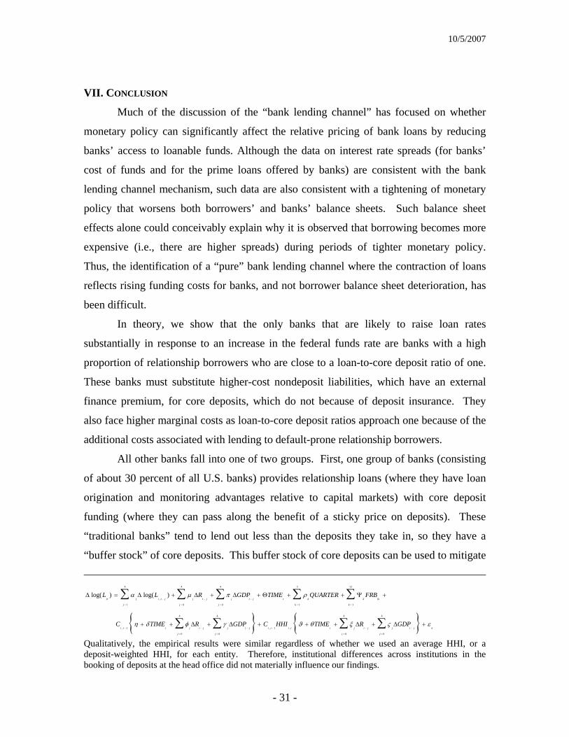
10/5/2007

- 31 -

VII. CONCLUSION

Much of the discussion of the “bank lending channel” has focused on whether

monetary policy can significantly affect the relative pricing of bank loans by reducing

banks’ access to loanable funds. Although the data on interest rate spreads (for banks’

cost of funds and for the prime loans offered by banks) are consistent with the bank

lending channel mechanism, such data are also consistent with a tightening of monetary

policy that worsens both borrowers’ and banks’ balance sheets. Such balance sheet

effects alone could conceivably explain why it is observed that borrowing becomes more

expensive (i.e., there are higher spreads) during periods of tighter monetary policy.

Thus, the identification of a “pure” bank lending channel where the contraction of loans

reflects rising funding costs for banks, and not borrower balance sheet deterioration, has

been difficult.

In theory, we show that the only banks that are likely to raise loan rates

substantially in response to an increase in the federal funds rate are banks with a high

proportion of relationship borrowers who are close to a loan-to-core deposit ratio of one.

These banks must substitute higher-cost nondeposit liabilities, which have an external

finance premium, for core deposits, which do not because of deposit insurance. They

also face higher marginal costs as loan-to-core deposit ratios approach one because of the

additional costs associated with lending to default-prone relationship borrowers.

All other banks fall into one of two groups. First, one group of banks (consisting

of about 30 percent of all U.S. banks) provides relationship loans (where they have loan

origination and monitoring advantages relative to capital markets) with core deposit

funding (where they can pass along the benefit of a sticky price on deposits). These

“traditional banks” tend to lend out less than the deposits they take in, so they have a

“buffer stock” of core deposits. This buffer stock of core deposits can be used to mitigate

{ } { }

4 4 4 3 12

,

1 0 0 1 1

4 4 4 4

, 1 , 1 ,

0 0 0 0

log( ) log( )it j i t j j t j j t j t k k ik

j j j k k

i t t j t j j t j i t i t t j t j j t j it

j j j j

L L R GDP TIME QUARTER FRB

C TIME R GDP C HHI TIME R GDP

α μ π ρ

η δ φ γ ϑ θ ξ ς ε

− − −

= = = = =

− − − − − −

= = = =

Δ = Δ + Δ + Δ + Θ + + Ψ +

+ + Δ + Δ + + + Δ + Δ +

∑ ∑ ∑ ∑ ∑

∑ ∑ ∑ ∑

Qualitatively, the empirical results were similar regardless of whether we used an average HHI, or a deposit-weighted HHI, for each entity. Therefore, institutional differences across institutions in the booking of deposits at the head office did not materially influence our findings.

10/5/2007

- 32 -

the full effect of tighter monetary policy on their bank-dependent borrowers. In this

manner, the business strategy of “traditional banks” acts as a “core deposit mitigation

channel” to provide funds to bank-dependent borrowers when there are monetary shocks.

In effect, there is no bank lending channel of monetary policy associated with these

traditional banks.

Second, another group of banks (also consisting of about 30 percent of all U.S.

banks) mainly relies on managed liabilities that are priced at market rates. These banks

do not have to shift from insured deposits to managed liabilities in response to tighter

monetary policy because their loans are already funded with managed liabilities. For

these banks as well, there is no unique bank lending channel of monetary policy.

Our empirical evidence is consistent with this stratification. We find evidence of

a bank lending channel for monetary policy only for banks that specialize in relationship

lending and also have a loan-to-deposit ratio near one – these banks significantly reduce

lending in response to a monetary contraction. For the other groups of banks, there is no

evidence of a bank lending channel.

Moreover, statistical importance is not economic importance. Although the banks

that reduce lending significantly in response to a monetary contraction account for almost

40 percent of U.S. banks, they hold only about six percent of U.S. banking assets.

Moreover, among these banks, only the ones with relatively low capital-to-asset ratios

seem to account for the bulk of the lending reduction. Thus, in the United States, the

bank lending channel seems limited in scope and importance, mainly because few banks

switch from core deposits to managed liabilities in response to changes in interest rates.

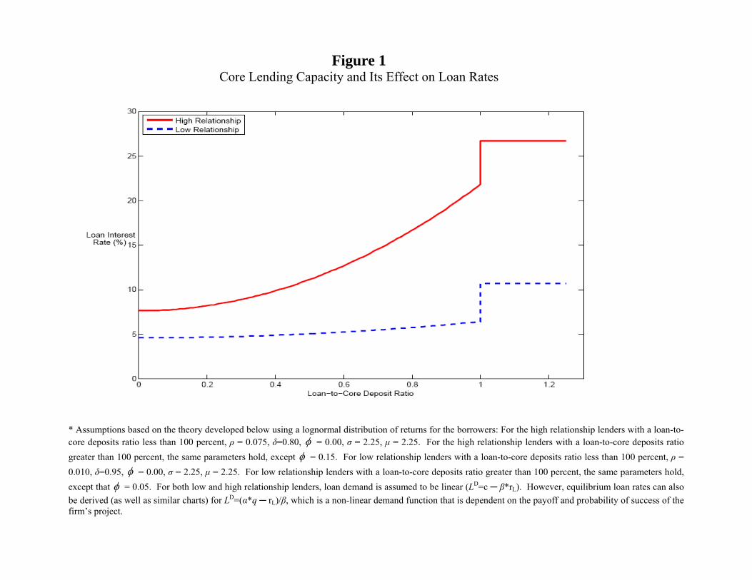
Figure 1 Core Lending Capacity and Its Effect on Loan Rates

* Assumptions based on the theory developed below using a lognormal distribution of returns for the borrowers: For the high relationship lenders with a loan-to-core deposits ratio less than 100 percent, ρ = 0.075, δ=0.80, φ = 0.00, σ = 2.25, μ = 2.25. For the high relationship lenders with a loan-to-core deposits ratio greater than 100 percent, the same parameters hold, except φ = 0.15. For low relationship lenders with a loan-to-core deposits ratio less than 100 percent, ρ = 0.010, δ=0.95, φ = 0.00, σ = 2.25, μ = 2.25. For low relationship lenders with a loan-to-core deposits ratio greater than 100 percent, the same parameters hold, except that φ = 0.05. For both low and high relationship lenders, loan demand is assumed to be linear (LD=c ─ β*rL). However, equilibrium loan rates can also be derived (as well as similar charts) for LD=(α*q ─ rL)/β, which is a non-linear demand function that is dependent on the payoff and probability of success of the firm’s project.

Figure 2 Effect of Core Lending Capacity on the Spread

* Assumptions based on the theory developed below using a lognormal distribution of returns for the borrowers: For the high relationship lenders with a loan-to-core deposits ratio less than 100 percent, ρ = 0.075, δ=0.80, φ = 0.00, σ = 2.25, μ = 2.25. For the high relationship lenders with a loan-to-core deposits ratio greater than 100 percent, the same parameters hold, except φ = 0.15. For low relationship lenders with a loan-to-core deposits ratio less than 100 percent, ρ = 0.010, δ=0.95, φ = 0.00, σ = 2.25, μ = 2.25. For low relationship lenders with a loan-to-core deposits ratio greater than 100 percent, the same parameters hold, except that φ = 0.05. For high relationship lenders, β = -0.01, and for low relationship lenders β = -2.00. For both low and high relationship lenders, loan demand is assumed to be linear (LD=c ─ β*rL). However, equilibrium loan rates can also be derived (as well as similar charts) for LD=(α*q ─ rL)/β, which is a non-linear demand function that is dependent on the payoff and probability of success of the firm’s project.

Figure 3Relationship Lending Intensity Score Cut-offs

0

0.1

0.2

0.3

0.4

0.5

0.6

0.7

0.8

1993

1994

1995

1996

1997

1998

1999

2000

2001

2002

2003

2004

2005

Year

RB

L/C

&I

Low Relationship Lender Intensity Score Cut-off High Relationship Lender Intensity Score Cut-off

In each year (2nd quarter), the high relationship lender intensity score cut-off is the 5th percentile of the RBL/C&I distribution and the low relationship lender intensity score cut-off is the 1st percentile of the RBL/C&I distribution.

Low Relationship Lenders

High Relationship Lenders

Medium Relationship Lenders

Figure 4Box Plots of Total Assets for Top Holders Stratified by Relationship Lender Status

(H=High, M=Medium, L=Low)(1993:Q2 - 2005:Q2)

Dolla

rs(0

00)

Year-Relationship Lender Group

Loan-to-Core Deposit Ratios by Relationship Lender Group Figure 5

25th Percentiles

0

0.2

0.4

0.6

0.8

1

1.2

1.4

1.6

1993

Q1

1993

Q3

1994

Q1

1994

Q3

1995

Q1

1995

Q3

1996

Q1

1996

Q3

1997

Q1

1997

Q3

1998

Q1

1998

Q3

1999

Q1

1999

Q3

2000

Q1

2000

Q3

2001

Q1

2001

Q3

2002

Q1

2002

Q3

2003

Q1

2003

Q3

2004

Q1

2004

Q3

2005

Q1

2005

Q3

Date

Rat

io o

f Loa

ns-t

o-C

ore

Dep

osits

Low Relationship Lenders Medium Relationship Lenders High Relationship Lenders

Medians

0

0.5

1

1.5

2

2.5

3

3.5

1993

Q1

1993

Q3

1994

Q1

1994

Q3

1995

Q1

1995

Q3

1996

Q1

1996

Q3

1997

Q1

1997

Q3

1998

Q1

1998

Q3

1999

Q1

1999

Q3

2000

Q1

2000

Q3

2001

Q1

2001

Q3

2002

Q1

2002

Q3

2003

Q1

2003

Q3

2004

Q1

2004

Q3

2005

Q1

2005

Q3

Date

Rat

io o

f Loa

ns-t

o-C

ore

Dep

osits

Low Relationship Lenders Medium Relationship Lenders High Relationship Lenders

75th Percentiles

0

2

4

6

8

10

12

1993

Q1

1993

Q3

1994

Q1

1994

Q3

1995

Q1

1995

Q3

1996

Q1

1996

Q3

1997

Q1

1997

Q3

1998

Q1

1998

Q3

1999

Q1

1999

Q3

2000

Q1

2000

Q3

2001

Q1

2001

Q3

2002

Q1

2002

Q3

2003

Q1

2003

Q3

2004

Q1

2004

Q3

2005

Q1

2005

Q3

Date

Rat

io o

f Loa

ns-t

o-C

ore

Dep

osits

Low Relationship Lenders Medium Relationship Lenders High Relationship Lenders

Relationship Lender GroupLess than 0.8 0.8 to 1.1 Greater than 1.1 Total

Proportion of All BanksHigh Relationship Lenders 0.286 0.376 0.290 0.951Medium Relationship Lenders 0.005 0.011 0.023 0.039Low Relationship Lenders 0.001 0.001 0.007 0.010 Total 0.291 0.388 0.320 1.000

High Relationship Lenders 0.300 0.395 0.305 1.000Medium Relationship Lenders 0.125 0.289 0.585 1.000Low Relationship Lenders 0.079 0.138 0.783 1.000

* Proportions are calculated on a bank-quarter basis.

Table 1

Proportion of Each Relationship Group

Proportional BasisLoan-to-Core Deposit Ratio Range

How Many Banks Are Core Lending Capacity Constrained?Proportion of Banks by Relationship Lender Status and by Range for the Loan-to-Core Deposit Ratio*

Less than 0.8 0.8 to 1.1 Greater than 1.1

High Relationship Lenders 0.014 -0.050 -0.0002(0.399) (0.005) (0.711)

Medium Relationship Lenders 0.066 0.025 -0.0009(0.639) (0.837) (0.687)

Low Relationship Lenders -0.343 0.450 0.0001(0.136) (0.119) (0.091)

Difference (High minus Low) 0.356 -0.500 -0.0003(0.083) (0.065) (0.580)

* Partial derivatives are evaluated at the sample means of the data.

Table 2Partial Derivatives of Bank C&I Lending Growth*

Loan-to-Core Deposit Ratio Range

Relationship Lender Group

with Respect to the Monetary Policy Indicator (R) and Core Lending Capacity (C) (P-Values in parentheses)

Less than 0.8 0.8 to 1.1 Greater than 1.1

High Relationship Lenders -0.746 -0.352 -0.018(<0.001) (<0.001) (<0.001)

Medium Relationship Lenders -0.731 -0.268 0.061(<0.001) (<0.001) (<0.001)

Low Relationship Lenders -0.842 -0.125 -0.012(<0.001) (0.017) (0.594)

Table 3The Relationship between Loan-to-Core Deposit Ratios and Securities-to-Assets Ratios

Loan-to-Core Deposit Ratio Range

Relationship Lender Group

Pearson Correlation Coefficients(P-Values in parentheses)

Relationship Lender Group Loan-to-Core Deposit Ratio Range Capital-to-Asset Ratio in the Bottom Quartile

High Relationship Lenders 0.80 < C < 1.1 -0.115 -0.028

(0.0005) (0.189)

* Partial derivatives are evaluated at the sample means of the data.

Does Bank Capitalization Matter for Core Lending Capacity Constrained Banks?Partial Derivatives of Bank C&I Lending Growth*

with Respect to the Monetary Policy Indicator (R) and Core Lending Capacity (C )

Capital-to-Asset Ratio in the Top Three Quartiles

Level of Capitalization

Table 4

Less than 0.8 0.8 to 1.1 Greater than 1.1

High Relationship Lenders -0.010 -0.006 -0.0006(0.219) (0.548) (0.768)

Medium Relationship Lenders -0.003 0.053 0.002(0.962) (0.364) (0.205)

Low Relationship Lenders -0.212 -0.213 0.0014(0.078) (0.292) (0.420)

Difference (High minus Low) 0.202 0.207 -0.0020(0.073) (0.291) (0.447)

* Partial derivatives are evaluated at the sample means of the data.

Table 5Partial Derivatives of Bank Mortgage Lending Growth*

with Respect to the Monetary Policy Indicator (R) and Core Lending Capacity (C) (P-Values in parentheses)

Relationship Lender Group

Loan-to-Core Deposit Ratio Range

10/5/2007

- 33 -

REFERENCES

Adams, R.M. and D.F. Amel, 2005, “The Effects of Local Banking Market Structure on the Bank Lending Channel of Monetary Policy,” Finance and Economics Discussion Series working paper, Federal Reserve Board, 2005-16, April.

Altunbas, Y., O. Fazylov, and P. Molyneux, 2002, “Evidence on the Bank Lending Channel in Europe,” Journal of Banking and Finance, 26, 2093-2110.

Berlin, M. and L.J. Mester, 1999, “Deposits and Relationship Lending,” The Review of

Financial Studies, 12, Fall, pp. 579-607. Bernanke, B.S. and A. Blinder, 1992, “The Federal Funds Rate and the Channels of

Monetary Transmission,” American Economic Review, September, 83(4), pp.902-21.

Bernanke, B.S. and M. Gertler, 1995, “Inside the Black Box: The Credit Channel of

Monetary Policy Transmission,” The Journal of Economic Perspectives, 9, Autumn, pp. 27-48.

Bernanke, B.S. and I. Mihov, 1998, “Measuring Monetary Policy,” Quarterly Journal of

Economics, August, 113(3), pp.869-902. Diamond, D.W. and R.G. Rajan, 2006, “Money in a Theory of Banking,” American

Economic Review, 96, 30-53. Freixas, X. and J. Jorge, 2007, “The Role of Interbank Markets in Monetary Policy: A

Model with Rationing,” working paper, Department of Economics and Business, Universitat Pompeu Fabra, June.

Gambacorta, L., 2005, “Inside the Bank Lending Channel,” European Economic Review,

49, 1737-59. Gatev, E. and P.E. Strahan, 2005, “Banks’ Advantage in Hedging Liquidity Risk: Theory

and Evidence from the Commercial Paper Market,” The Journal of Finance, 61, April, pp. 867-892.

Hannan, T.H. and A.N. Berger, 1991, “The Rigidity of Prices: Evidence from the

Banking Industry,” The American Economic Review, 81, September, pp. 938-945.

Houston, J.F. and C. James, 1998, “Do bank internal capital markets promote lending?” Journal of Banking and Finance, 22, pp. 899-918.

Houston, J.F., C. James, and D. Marcus, 1997, “Capital market frictions and the role of internal capital markets in banking,” Journal of Financial Economics, 46, pp. 135-64.

10/5/2007

- 34 -

Hubbard, R.G., K.N. Kuttner, and D.N. Palia 2002, “Are There Bank Effects in Borrowers’

Costs of Funds? Evidence from a Matched Sample of Borrowers and Banks,” Journal of Business, 75, October, pp. 559-581.

Jayaratne, J. and D.P. Morgan, 2000, “Capital Market Frictions and Deposit Constraints at

Banks,” Journal of Money, Credit, and Banking, 32, pp. 74-92. Kahn, C., G. Pennacchi, and B. Sopranzetti, 1999, “Bank Deposit Rate Clustering:

Theory and Empirical Evidence, The Journal of Finance, 54, December, pp. 2185-2214.

Kashyap, A.K., R.G. Rajan, and J.C. Stein, 2002, “Banks as Liquidity Providers: An

Explanation for the Coexistence of Lending and Deposit-taking,” The Journal of Finance, 57, February, pp. 33-73.

Kashyap, A.K. and J.C. Stein, 1995, “The Impact of Monetary Policy on Bank Balance

Sheets,” Carnegie-Rochester Conference Series on Public Policy, June, pp. 151-195.

Kashyap, A.K. and J.C. Stein, 2000, “What Do a Million Observations on Banks Say

about the Transmission of Monetary Policy?” The American Economic Review, 90, June, pp. 407-428.

Kishan, R., and T. Opiela, 2000, “Bank size, bank capital, and the bank lending channel,”

Journal of Money, Credit, and Banking, 32, pp. 121-41. Kishan, R., and T. Opiela, 2006, “Bank Capital and Loan Asymmetry in the Transmission

of Monetary Policy,” Journal of Banking and Finance, 30, pp. 259-85. Neumark, D. and S.A. Sharpe, 1992, “Market Structure and the Nature of Price Rigidity:

Evidence from the Market for Consumer Deposits,” The Quarterly Journal of Economics, 107, May, pp. 657-680.

Peek, J. and D. Holod, 2006, "The Value of Banks of Small Business Lending," Working paper, University of Kentucky, September. Petersen, M.A. and R.G. Rajan, 1995, “The Effect of Credit Market Competition on

Lending Relationships,” Quarterly Journal of Economics, 110, May, pp. 407-443. Romer, C.D. and D. Romer, 2004, “A New Measure of Monetary Policy Shocks:

Deivation and Implications,” American Economic Review, 94(4), September, pp.1055-1084.

Van den Heuvel, S.K., 2007, “The Bank Capital Channel of Monetary Policy,” working

paper, The Wharton School, University of Pennsylvania, June.