Bank Bailouts, Bail-ins, or No Regulatory Intervention? ADynamic Model and Empirical Tests of Optimal Regulation ∗

Allen N. Berger †

University of South CarolinaWharton Financial Institutions Center

European Banking Center

Charles P. Himmelberg ‡

Goldman Sachs & Co.

Raluca A. Roman §

Federal Reserve Bank of Philadelphia

Sergey Tsyplakov ¶

University of South Carolina

August 6, 2018

Abstract

We develop and test a dynamic model of optimal regulatory design of three regimes todeal with distress of large banking organizations. These are 1) bailout, as under TARP;2) bail-in, as under Orderly Liquidation Authority; and 3) no regulatory intervention, asunder Financial CHOICE Act. We find that no regulatory intervention is suboptimalrelative to the other two regimes and that only bail-in provides incentives for banksto rebuild capital preemptively during distress. Empirical tests of changes in capitalratios and speeds of adjustment when shifting from the pre-crisis bailout regime to thepost-crisis bail-in regime corroborate model predictions.

JEL Classification Codes: G21, G28

Keywords: Banks, Bailouts, Bail-ins, OLA, Bankruptcy, Regulation, Capital Struc-ture.

∗The views expressed are those of the authors and do not necessarily reflect the views of the Federal ReserveBank of Philadelphia, the Federal Reserve System, or Goldman Sachs & Co. Part of the theoretical model work wascompleted while Sergey Tsyplakov was a visiting scholar in the Global Investment Research division at Goldman Sachs.The authors thank Stijn Claessens, Bill English, Tim Landvoigt, Robert Marquez, Ettore Panetti, Zhenyu Wang,and participants at the 1st Biennial Bank of Italy and Bocconi University Conference on ”Financial Stability andRegulation,” the 2018 Yale School of Management Conference on ”The Financial Crisis Ten Years Afterwards,” the2018 University of South Carolina Fixed Income and Financial Institutions Conference, the 2018 European FinancialManagement Association Meetings, and University of South Carolina, Case Western University, and Higher Schoolof Economics in Moscow seminars for very helpful comments, and Rose Kushmeider and Jack Reidhill for helpfulbackground information on the Orderly Liquidation Authority (OLA).

†Darla Moore School of Business, University of South Carolina, Columbia, SC 29208; E-mail:aberger@moore.sc.edu.

‡Goldman Sachs & Co., 200 West Street, New York, NY 10282; E-mail: charles.himmelberg@gs.com.§Federal Reserve Bank of Philadelphia, Risk Assessment, Data Analysis, and Research Group, Ten Independence

Mall, Philadelphia, PA 19106, E-mail: raluca.roman@phil.frb.org.¶Darla Moore School of Business, University of South Carolina, Columbia, SC 29208; E-mail:

sergey@moore.sc.edu.

”I was never able to convince the American people that what we did with TARP was not for thebanks. It was for them. It was to save Main Street. It was to save our economy from a catastrophe.”(Henry Paulson, former Secretary of the Treasury, Five Years from the Brink, BloombergBusinessWeek, Sep 2013).

”Eliminating OLA would be a major mistake because these are essential tools for ensuring that financialstress does not escalate into a catastrophic crisis. We saw what happens without OLA. We saw it...it’s2008. We don’t want that again.” (Ben Bernanke, former Chairman of the Federal ReserveSystem 2006-2014, Remarks at the Brookings Institution Falk Auditorium on Is Dodd-Frank’s Failure Resolution Regime Failing?, Jun 2017)

”Every promise of Dodd-Frank has been broken...Fortunately there is a better, smarter way. It’s calledthe Financial Choice Act. It stands for economic growth for all, but bank bailouts for none. We will endbank bailouts once and for all. We will replace bailouts with bankruptcy.” (Jeb Hensarling, FinancialServices Committee Chairman, Press Releases, House Approves Financial Choice Act toBoost Economy, End Bank Bailouts and Toughen Penalties for Fraud, Jun 2017).

1 Introduction

As seen in the financial crisis of 2007-2009, the failure of large, complex financial institutions (e.g.,

Lehman Brothers) can cause or worsen a financial crisis, threaten the financial system, and cause

large real economic losses. To mitigate such problems, regulators design regimes for handling the

financial distress and impending potential failure of large banking organizations. In particular,

when the capital ratios of such institutions reach critically low levels, regulators decide among

regimes of 1) bailouts, government injections of capital; 2) bail-ins, private sector injections of

capital; or 3) no regulatory intervention, allowing the institutions to fail.

Coupled with these regimes, regulators employ other prudential regulatory tools as “first lines

of defense” to reduce the chances that the institutions become financially distressed and trigger the

resolution regimes. Such tools include traditional capital standards that impose capital minimums

based on historical patterns, and stress tests that base capital minimums on forward-looking adverse

scenarios. These tools often come with restrictions on financial institutions that fail to meet the

standards, such as limits on dividends and share buybacks.

These resolution regimes are key topics of debate, as witnessed by the quotes above that defend

each of the three regimes. Prior to the financial crisis, most large, complex U.S. bank holding

companies (BHCs) likely perceived that they were in a bailout regime, which was actualized by

the Troubled Asset Relief Program (TARP) and other bailouts during the crisis. After the crisis,

the Dodd-Frank Act of 2010 imposed the Orderly Liquidation Authority (OLA), a type of bail-in

1

in which shareholders of distressed institutions lose their shares and junior debtholders have some

or all of their debt claims turned into equity capital. The Financial CHOICE Act – which would

replace OLA with a no-regulatory-intervention regime of bankruptcy for large BHCs – is currently

under congressional consideration. In February 2018, the U.S. Treasury recommended keeping OLA

for the largest institutions, and making bankruptcy easier for others.

Researchers and practitioners recognize structural differences among these regimes. However,

there is no consensus on how these regimes should be optimally designed, and how aggressive these

regimes should be in taking actions against distressed banks, such as intervening at relatively high

or low bank capital ratios. Nor is there an agreement on the relative benefits of each regime.

Addressing these questions requires not only static analysis of the ex post consequences of the

regimes, but also dynamic analysis of how the anticipation of bailout, bail-in, and no regulatory

intervention affects the ex ante behavior of the financial institutions. These regimes may differ in

the incentives they generate for the institutions to manage their own capital to avoid regulatory

intervention or default.

We contribute to these debates by dynamically modeling the regimes and empirically testing

the model’s implications. We explicitly model one single BHC which owns one bank. BHCs

choose their initial capital structures – bank capital and senior debt, BHC shareholders’ equity,

and subordinated debt – in response to the three regulatory regimes, as well as any subsequent

recapitalization decisions. In the model, the representative bank’s asset value is stochastic and

subject to infrequent negative random jumps or sudden falls in capital, such as those due to

financial crises. These jumps may result in regulatory interventions or default.

In the bailout regime, regulators inject equity capital and acquire a fair-priced partial stake when

the bank’s capital falls to some critical distress level. Under bail-in, existing BHC shareholders’

equity is wiped out and subordinated debt converts to BHC shares, possibly at a loss. For both

of these regimes, regulators optimize for each BHC the trigger points – the capital ratios at which

interventions occur. Finally, under no regulatory intervention, the BHC is allowed to fail. To

mimic the regulatory environment, we also incorporate stress tests into bail-in and no-regulatory-

intervention regimes. If the bank’s capital ratio falls below the stress test critical capital ratio (i.e.,

fails the stress test), the BHC has to suspend dividends and retain earnings to rebuild its capital.

In response to the prevailing regime, the BHC maximizes its own private value by endogenously

choosing its initial capital structure. It also dynamically adjusts its capital ratio over time, choosing

2

whether and at what capital ratio it raises additional equity to avoid bailout, bail-in, or default.

In designing socially optimal policies, the regulator maximizes a very simple social welfare

function that balances the benefits of the efficient provision of financial services by large financial

institutions with costs of disruptions to the financial system and the real economy associated

with the failure of these institutions. Motivated by this objective, we assume that the regulator

maximizes the value of the BHC minus the expected external social costs from its default. In

doing so, regulators take into account the self-optimizing responses of the BHC. Each of the three

regimes is optimally designed to use the tools at hand (bailout, bail-in, stress test) to incentivize the

BHC to make capital structure decisions that enhance financial system stability without significant

harming their private values.

The model is calibrated to be roughly consistent with the observed characteristics of large U.S.

BHCs prior to and after the financial crisis. We calculate and compare optimally-designed pure-

play bailout, bail-in, and no-regulatory-intervention regimes, assuming that the BHC chooses its

optimal capital structure strategies to maximize shareholder value for each of the regimes.

We find that the optimally-designed bailout and bail-in regimes attain comparable values of

social welfare function and both dominate the no-regulatory-intervention regime, suggesting that

more intrusive regulatory policies of bailouts and bail-ins are more effective in reducing chances of

bank failures than the stress test alone that is employed in the no-regulatory-intervention regime.

However, bailouts produce somewhat lower social welfare values than bail-ins if the costs of us-

ing and risking taxpayers’ funds and transaction costs of raising and distributing these funds are

incorporated in the social welfare function.

Several other factors also favor bail-ins over bailouts. Both the dynamic model and the em-

pirical results suggest that bail-ins provides BHCs better incentives to hold higher capital and to

recapitalize during financial distress, resulting in a safer banking industry. We also find that the

optimal trigger for the bail-in regime occurs at a higher capital ratio than for the bailout regime,

providing strong incentives for the BHCs to choose higher capital ratios and manage their capital

more prudently under the bail-in regime.

Our findings demonstrate that the optimal resolution design requires a delicate balance. For

example, a bail-in regime should not be too aggressive, i.e., should not intervene at such a high

capital ratio as to inefficiently constrain bank’s activity. However, it needs to be aggressive enough

to provide incentives that promote socially prudent behavior.

3

Another implication is that a “one size fit all” resolution design is suboptimal. Instead, reg-

ulators should implement regulations on a case-by-case basis that reflect each BHC’s individual

characteristics. For a given regime and set of bank characteristics, there are interior solutions for

both the optimal regulatory trigger and the stress test critical capital ratio that maximizes social

value. Thus, each regime should allow for regulatory discretion in setting triggers across BHCs, as

opposed the same rules uniformly applied to all institutions.

Importantly, several of the outcomes are unique to the dynamic model, and go beyond the limits

of static models. For example, the effects of high asset volatility on the optimal bailout trigger

are directly opposite to the effects on the optimal bail-in trigger. In our model, the regulator is

optimally less aggressive under the bailout regime for banks with more volatile assets, triggering

bailouts at lower capital ratios than for those with less volatile assets. In contrast, for bail-ins, the

regulator is optimally more aggressive for banks with higher asset volatility. The main reason is

that the two regimes structurally differ in the incentives they create for BHCs. Higher volatility

increases the debt overhang problem, which can reduce the BHCs’ incentive to preemptively raise

capital to avoid wiping out shareholders, necessitating more aggressive optimal bail-in for these

BHCs. This argument does not apply for bailouts, which provide no incentives for BHCs to rebuild

their own capital. Such findings cannot be derived from a static model in which the optimal dynamic

adjustments of BHCs’ capital structures in response to regulation are not taken into account.

Another model implication is that when the regime shifts from bail-in to no regulatory inter-

vention, the BHCs optimally responds by increasing capital. This implication is again inconsistent

with static intuition, under which the threat of being “wiped out” in bail-in resolution implies

higher initial capital. In contrast, in the dynamic model, the BHC endogenously pre-commits to

rebuild capital in response to negative shocks in the bail-in regime. This pre-commitment leads to

lower costs of debt, higher debt capacity, lower initial capital, and larger tax shields. In contrast,

the no-regulatory-intervention regime provides no such pre-commitment.

We acknowledge several limitations of our model. First, we deliberately abstract from regulatory

ambiguity and assume that all agents know which regime is in place. The purpose is to see which

pure-play regime is best in terms of maximizing social value. We recognize that some regulatory

ambiguity is unavoidable in practice.

The model may also overstate the net social benefits of the bailouts by assuming that bailouts

occur in a timely fashion that avoids direct subsidies or “free money” to failing institutions. When

4

public funds are injected, the regulator takes a fair-market stake in the bank, which leads to dilution

of the existing shareholders. In practice, however, bailouts are often executed too late and subsidize

bank shareholders at taxpayer expense. In addition, the model may understate the social benefits

of the bail-in regime relative to bailouts by focusing only on capital structure decisions. The bail-in

regime may have additional benefits in terms of reducing incentives to shift into riskier assets, and

lessening unfair competitive advantages of banks that are too big or interconnected to fail. While

these other effects are important, they cannot all easily be incorporated into a single comprehensive

dynamic model.6

Finally, the stress tests in our model are a combination of actual stress tests and capital stan-

dards. They combine the restrictions on dividend payments and share buybacks of stress tests and

the minimum requirements of capital standards. We do not model the forward-looking adverse

scenarios of the real-world stress tests because they are difficult to incorporate in our dynamic

model and would detract from our main focus on resolution regimes.

We empirically test a number of model predictions. Specifically, we test how well BHC capital

decisions correspond to the predictions about shifting from a bailout to a bail-in regime using the

observed shift from the bailout period before the financial crisis to the bail-in period after the

financial crisis.

For these tests, we specify 2000:Q3 to 2007:Q2 as the bailout period, when the largest U.S.

BHCs likely expected that they would be bailed out in the event of severe financial distress. We

use the time after the passage of the Dodd-Frank Act put OLA into effect from 2010:Q3 to 2017:Q2

as the bail-in period. We exclude the tumultuous period of the financial crisis itself in which the

bailouts actually occurred from the empirical analysis.

We use quarterly financial data for the top 50 publicly traded U.S. BHCs during the bailout

and bail-in periods. We consider the eight large, complex U.S. banking organizations designated as

Globally Systemic Important Banks (G-SIBs) as the treatment group most likely to be subject to

bailouts and bail-ins, and the remaining 42 BHCs as the control group. As argued in the empirical

section below, our empirical approach is based on the assumption that these G-SIBs were more

likely to expect bailouts than the other BHCs prior to the financial crisis and more likely than

6To illustrate, Veronesi and Zingales (2010) and Glasserman and Wang (2015) find subsidies to TARP bailouts’recipients, and Tsesmelidakis and Merton (2013) find subsidies to financial institutions that are considered “too bigto fail” in terms of cheaper funding costs.

5

the others to expect bail-ins after Dodd Frank. We recognize that this division is imperfect. In

robustness tests, we experiment with alternative treatment and control groups, and the results are

largely robust.

We test the model predictions that in moving from the bailout period to the bail-in period,

the treated G-SIB group raised their capital ratios more and increased their speeds of adjustment

toward target capital ratios more than the control group. The data are consistent with both

predictions, and line up remarkably well with the quantitative predictions of the model as well. For

example, the model base case predicts a 2.7 percentage point increase in the BHC’s optimal capital

ratio when moving from the bailout to the bail-in regime, while the difference-in-difference empirical

results show 1.0 to 2.7 percentage point increases in the G-SIBs capital ratios relative to the control

group moving from pre-crisis to post-crisis. Similarly, our empirical results for speed of adjustment

toward target capital ratios show that G-SIBs more than doubled their adjustment speeds post-

crisis, while the control group BHCs did not significantly change their adjustment speeds, consistent

with model predictions that the bail-in regime provides incentives to recapitalize.

The remainder of the paper is organized as follows. Section 2 briefly discusses our contributions

to the theoretical and empirical literatures. Section 3 provides information on regulatory environ-

ments of the past, present, and potential future to put the paper into context. Section 4 presents

the dynamic model of the three regimes, giving a timeline, followed by model implications and

empirical predictions. Section 5 offers our empirical analysis, and Section 6 contains conclusions

and policy implications. Appendix A presents the analytics of the model solution, and Appendix

B gives additional empirical results.

2 Contributions of the Paper

We add to the theoretical and empirical literatures on regulatory resolution regimes. Some theory

papers use dynamic continuous-time models to tackle related issues. Hugonnier and Morellec (2017)

show that banking organizations facing minimum liquidity and leverage requirements choose more

reserves and higher capital, lowering the likelihood of default and reducing losses given default.

Sundaresan and Wang (2016) examine optimal leverage choices when facing runs and closure.

They find that institutions optimally set the levels of subordinated debt and capital such that the

endogenous default boundary coincides with closure boundary. Unlike these papers, we examine

6

the effects of bailout, bail-in, and no-regulatory-intervention regimes, and the transitions between

regimes. Another key contribution is that we analyze the optimal terms of the regulatory regimes.

There are also several static models of optimal regulatory interventions. Philippon and Schnabl

(2013) solve for the optimal regulatory intervention via equity injection to reduce a debt overhang

problem. Farhi and Tirole (2012) also characterize optimal regulation, including minimum liquidity

requirements and restrictions on liquid assets. Allen, Carletti, Goldstein, and Leonello (2017)

consider an equilibrium model in which bank runs and depositors’ decisions are endogenously

determined by the amount of government guarantees. In contrast to these static models, our model

is dynamic, and allows for BHC’s capital structure to be endogenously determined, depending on

the “aggressiveness” of the regulatory interventions. Thus, we model the optimal responses of the

BHCs to the regulatory regimes, and form the optimal regulatory regimes based on these optimal

responses of the BHCs.

Turning to the empirical literature, we contribute to the findings on banking capital structure

determinants by analyzing the effects of the different regulatory regimes and prudential regulatory

tools. This literature finds that in addition to regulation, BHCs’ capital structures are influenced

by financial factors (e.g., Berger, DeYoung, Flannery, Lee, and Oztekin, 2008) and governance

pressures from other stakeholders (e.g., Flannery and Sorescu, 1996; Morgan and Stiroh, 2001;

Martinez Peria and Schmuckler, 2001; Calomiris and Wilson, 2004; Ashcraft, 2008; Flannery and

Rangan, 2008; Lepetit, Saghi-Zedek, and Tarazi, 2015).

We also add to the empirical findings on bailouts, most of which focus on the U.S. TARP

program. Most of the findings suggest increases in credit supply from the TARP bailouts (e.g.,

Berrospide and Edge, 2010; Black and Hazelwood, 2013; Li, 2013; Duchin and Sosyura, 2014; Puddu

and Walchli, 2015; Bassett and Demiralp, 2016; Chavaz and Rose, 2017; Berger and Roman, 2017;

Chu, Zhang, and Zhao, forthcoming). The results also suggest improved real economic outcomes

(Berger and Roman, 2017), increases in individual institution risk (e.g., Black and Hazelwood,

2013; Duchin and Sosyura, 2014), but reductions in systemic risk due to the increases in bank

capital (Berger, Roman, and Sedunov, 2018).

Finally, we add to the empirical literature on bail-ins, which is mostly focused on Europe, where

bail-ins have occurred. This research finds that bail-ins increase market discipline by depositors,

bondholders, stockholders, and CDS holders (Schafer, Schnabel, and Weder, 2016; Boccuzzi and

De Lisa, 2017; Giuliana, 2017; Bonfim and Santos, 2018; Brown, Evangelou, Stix, 2018; Neuberg,

7

Glasserman, Kay, and Rajan, 2018). Some also find reduced systemic risk and greater taxpayer

protection (e.g., Pellerin and Walter, 2012; Conlon and Cotter, 2014; Avgouleas and Goodhart,

2015; Klimek, Poledna, Farmer, and Thurner, 2015). However, others report undesirable conse-

quences including increased stock market volatility (Leone, Porretta, and Riccetti, 2017), problems

in handling simultaneous insolvencies of several large banks and international cooperation (e.g.,

Persaud, 2014; Mitts, 2015; Avgouleas and Goodhart, 2016; Hadjiemmanuil, 2016). Still others

find harm for households that own deposits and subordinated debt at bailed-in banks (Pigrum,

Reininger and Stern, 2016; Zenios, 2016; Boccuzzi and De Lisa, 2017) bank borrowers and other

connected stakeholders (e.g., Beck, Da-Rocha-Lopes, and Silva, 2017).

In contrast to these studies of actual bailouts and bail-ins, our empirical analysis focuses on the

effects of expectations of bailouts pre-crisis and expectations of bail-ins after the Dodd Frank Act

imposed OLA on the capital structures of the BHCs most likely to be subject to bailouts and bail-

ins. This setup allows us to test the implications of the dynamic theoretical model, which predicts

higher bank capital ratios and faster adjustments toward target capital ratios under expectations

of bail-in than expectations of bailout. As noted, our empirical results are highly consistent with

the predictions of the theoretical model.

3 Background on Regulatory Regimes

To put the paper in context, we provide background information on four time periods in the U.S.

with different regulatory regimes – the pre-crisis bailout regime, the crisis period in which the

bailouts were realized, the post-crisis bail-in period, and the potential future period in which no

regulatory intervention might prevail.

3.1 Pre-Crisis Bailout Regime

Prior to the financial crisis, large U.S. BHCs likely had reasonable expectations that they were

too big to fail and were likely to be bailed out, rather than undergo no regulatory intervention.

Bail-in was not a possibility under the laws at that time. All U.S. BHCs were subject to the

Basel I risk-based capital standards and non-risk-based leverage requirements. They were also

subject to the Prompt Corrective Action (PCA) rules of the FDIC Improvement Act of 1991,

which specifies mandatory and discretionary actions to be taken by regulators as capital fell below

8

various trigger points. Under least-cost resolution policies, the FDIC is required to resolve critically

undercapitalized institutions capital ratios below 2% by means that minimize the present value of

net long-term losses to the FDIC.7

While the banking system performed relatively well for a long period of time, PCA rules were

not strictly followed and no large commercial banking organizations were closed, potentially due to

systemic risk considerations (e.g., Dell’Ariccia, Detragiache, and Rajan 2008; Correa, Lee, Sapriza,

and Suarez, 2014).

3.2 Financial Crisis Period in which Bailouts Occurred

During the crisis, expectations of bailouts of large BHCs in financial distress were realized. Among

the many assistance programs, the U.S. Treasury TARP injected more than $200 billion in preferred

equity capital into 709 financial institutions through the Capital Purchase Program (CPP), with

most of the funds going to the largest eight BHCs, all of which were required to participate. Each

institution received 1% to 3% of its risk-weighted assets or $25 billion, whichever was smaller.8

3.3 Post-Crisis Bail-in Regime

After the crisis, the Dodd-Frank Act introduced the Orderly Liquidation Authority (OLA). OLA

is triggered for a large BHC when the Treasury Secretary, in consultation with the President, as

well as two-thirds of the Federal Reserve and FDIC boards, finds that the BHC is in default or

danger of default, and its failure would have serious adverse financial stability consequences. The

critical point of distress may be due to a severe capital shortfall, a liquidity problem, or both.

When OLA is triggered, the FDIC temporarily takes over the BHC and fires its management,

while banks and other holding company subsidiaries continue to operate. There is also a bail-in

in which shareholders are wiped out and subordinated debtholders and possibly other uninsured

creditors have part of their debt claims turned into equity capital, so that the BHC becomes well

capitalized. The BHC is then returned to private hands with new management.9

7For more details for the FDIC resolution process see https://www.fdic.gov/bank/analytical/banking/2001sep//article1.html and https://www.fdic.gov/bank/historical/managing/history1-02.pdf.

8Other bailouts during the crisis include expanded access to Federal Reserve liquidity through the discountwindow and Term Auction Facilities (TAF), Federal Reserve quantitative easing (QE) programs, and additional bankguarantees provided by the Federal Deposit Insurance Corporation (FDIC).

9See Pellerin and Walter (2012) for details on OLA.

9

The crisis also resulted in the U.S. stress tests, the 2009 Supervisory Capital Assessment Pro-

gram (SCAP), and the current Comprehensive Capital Analysis and Review (CCAR), and Dodd-

Frank Act Stress Tests (DFAST). These are essentially forward-looking capital requirements in-

tended to ensure that large banking organizations have sufficient capital to remain viable and con-

tinue lending even under future adverse conditions (quantitative assessment), and ensure adequate

risk management (qualitative assessment).

During the post-crisis period, Basel III capital standards are phased in between January 2013

and January 2019, which apply to all U.S. BHCs with assets over $500 million. These standards

represent an increase in required capital. There are also capital conservation buffers that raise the

effective capital ratios higher, as well as add-ons for all 30 G-SIBs, including eight large U.S. BHCs.

3.4 Potential Future No-Regulatory-Intervention Regime

The Financial CHOICE Act, H.R.10 of the 115th Congress, was introduced in the U.S. House

of Representatives on April 26, 2017 by Representative Jeb Hensarling, and passed the House on

June 8, 2017. It would repeal certain provisions of the Dodd-Frank Act of 2010 and other laws. In

particular, the CHOICE Act would repeal OLA and allow the FDIC to liquidate a failing financial

institution if the institution’s imminent failure threatens financial stability. It would establish

Chapter 11 bankruptcy for large, complex financial institutions, and under some circumstances

convert them into Chapter 7 liquidation bankruptcy.10

4 Model

4.1 Model description and time line

We model a bank’s dynamic capital structure under three regulatory regimes – bailout, bail-in, and

no regulatory intervention. Bank’s asset values are stochastic and described by a jump-lognormal

process. Random negative jumps of stochastic size are infrequent, representing severe runs or

financial crises. Bank cash flows are proportional to assets. Dividends are calculated as a residual

cash flow after interest payments, and interest payments are tax deductible.

10For more details on the Financial CHOICE Act, see https://www.congress.gov/bill/115th-congress/house-bill/10.

10

At time 0, the bank issues senior debt and capital, where the bank capital is owned by its

BHC. The bank’s capital ratio is the ratio of equity to total assets. The BHC can issue both its

own shareholders’ equity and subordinated debt to finance the bank’s capital, often referred to as

double leverage.

The capital structures of a representative bank and its holding company are shown in Figure 1

(the figure is not drawn to scale to ease exposition). The bank’s capital structure is shown on the

left with the 9% of assets financed by capital and 91% by senior debt, roughly corresponding to

ratios observed for typical large banks. The right side shows an amalgam of the capital structure

of the bank and the BHC that owns it, in which the BHC’s shareholders’ equity and subordinated

debt are superimposed over the bank’s capital. In this case, the 9% bank capital ratio is funded

by 7% shareholders’ equity and 2% subordinated debt.

Both subordinated and senior debt require continuous coupon payments and have the same

maturity, but the subordinated debt is junior and absorbs losses first if the bank defaults or is

bailed in. At maturity, par values are paid to claimants if neither restructuring nor default have

not occurred in prior periods. Following Leland (1994) and Titman and Tsyplakov (2005), we

assume that a certain fraction of bank’s senior liabilities is continuously repaid at par and reissued

at market price, such that the principal value remains unchanged. This structure reflects the

fact that in practice, liabilities of large banks are combinations of short- and long-term deposits,

overnight federal funds, term wholesale deposits and repo financing instruments, which are rolled

over. The higher the rollover rate, the shorter is the effective maturity of senior liabilities relative

to subordinated debt. For simplicity, we assume that the rollover rate is constant.

At time 0, the regulator announces that the regulatory regime is bailout, bail-in, or no regulatory

intervention. In regimes with stress tests (bail-in and no regulatory intervention), the regulator

also specifies a minimum capital requirement below which the bank cannot pay dividends and

must retain earnings to rebuild its capital. We assume no regulatory ambiguity – the regulator

pre-commits to the trigger point at which the bailout or bail-in will occur for each individual bank

as well as the minimum capital requirement.

In anticipation of expected future regulatory interventions, the BHC chooses the bank’s capital

ratio, and the size of BHC subordinated debt. We assume that subordinated debt remains a

constant percentage of total debt through time. The initial capital of the bank is chosen to maximize

the market value of the BHC, i.e., the total market value of the equity, senior liabilities and

11

subordinated debt reaches its maximum. After time 0, the bank can raise equity (of any size)

multiple times before maturity to move away from trigger or default boundaries. When the bank

raises equity capital, it incurs transaction costs with fixed and variable components. The strategy

of raising capital is endogenous and chosen to maximize the existing shareholders’ equity.

In the bailout regime, the regulator steps in and injects equity capital when the bank’s capital

ratio declines to or below the trigger point. Consistent with the TARP program discussed in Section

3, we assume that the regulator injects 2% equity as a fraction of the bank assets, and takes a fair

market stake in the bank’s equity, diluting the claims of the existing shareholders. The shareholders

do not incur any transaction costs for the equity injected by the regulator. Notably, in the case of

a very large jump, existing shareholders may be wiped out and the market value of the regulator’s

equity stake might be less than the amount injected. The regulator can bail out the bank multiple

times.

Figure 2A illustrates the sequence of events for the bailout regime (again not drawn to scale).

It shows on the left the initial capital structure of the BHC, followed by the middle which shows

the capital structure after a negative shock that reduces capital to the trigger. We use a bailout

trigger of 2.9% capital ratio here, which turns out to be socially optimal for our base case discussed

below. The right part of the figure shows the capital structure after the regulator injects equity of

2%.

In the bail-in regime, the regulator steps in as soon as the bank capital ratio declines to or below

the predetermined trigger, and the existing shareholders’ equity is wiped out. Subordinated debt

converts to bank shares at fixed market value. The face value of subordinated debt determines the

market value of equity to be owned by subordinated debt holders (could be potentially below par),

where the exact number of new shares is calculated after bail-in intervention.11 After bail-in, the

bank continues to operate until maturity or default. Figure 2B illustrates the sequence of events

for the bail-in regime. As above, the left part shows the initial capital structure. As shown in the

middle and right part of the figure, in response to the negative shock, the regulator intervenes and

wipes out existing equity, as well as converts the subordinated debt to equity. The socially optimal

bail-in trigger of 3.6% capital ratio shown in the figure (as derived in the model below) is higher

than the socially optimal bailout trigger.

11The remaining market value of equity stake (if any) will be owned by the regulator.

12

For the no-regulatory-intervention regime, bankruptcy occurs without intervention. We assume

that the BHC files for bankruptcy, when the shareholder’s equity declines to zero. In case of

default, the BHC is liquidated, shareholders are wiped out, subordinated debt holders are partially

or fully wiped out, and the holders of senior liabilities recover the bank’s unlevered assets minus

proportional default costs. Figure 2C shows the no-regulatory-intervention regime. Regulators

allow the BHC to be liquidated and the senior debtholders recover bank assets minus default costs.

For the bailout and bail-in regimes, if asset values fall instantly below book value of senior debt

due to the arrival of a large negative jump, the bank is classified as in technical default. For such

cases, we assume that the regulator is not able to intervene, the bank defaults, and the BHC is

liquidated. Shareholders and subordinated debt holders are wiped out, and the holders of senior

liabilities recover the bank assets minus default costs.

To mimic the regulatory regime observed after the crisis (see Section 3), we assume that in the

bail-in and no-regulatory-intervention regimes, the regulator also conducts stress tests. BHCs that

fail the tests (i.e., if its capital ratio declines below the critical level) eliminate dividends to retain

earnings and build capital. We assume no uncertainty about the capital ratio set by the stress

tests. These stress tests mimic a combination of actual stress tests and capital standards to allow

us to focus on the resolution regimes.

The model quantifies socially-optimal terms of each regulatory regime, including the combina-

tion of the critical trigger capital ratios at which the regulator intervenes as well as the stress test

parameters. Consistent with observations from the financial crisis, we assume that bank failures

create negative externalities for the financial system through interconnections and contagion that

make other banks more vulnerable to losses. The regulator socially optimizes by maximizing the

value of the bank minus the expected value of the negative externalities from default. In our base

case specification, we assume that the external cost of bank default is moderate – a multiple of

one times the expected default costs to the bank stakeholders. This weighting scheme effectively

assumes that for every $1 of expected costs of default to bank stakeholders, an additional $1 is

imposed on the rest of the financial system and the real economy.We also conduct a sensitivity

analysis in which this multiple is relatively small, such as for a failure of a smaller institution (0.5

times expected bank default costs), and relatively large, such as for a Lehman-like failure (10 times

expected bank default costs).

13

4.1.1 Value of bank assets

We assume that the bank’s assets follows a log-normal stochastic process with random negative

jumps with a stochastic jump size. The arrival of the jump discontinuously reduces the value of

the bank’s assets.12 Jumps such as runs or financial crises represent a real-world “frictions” that

preclude the possibility of the firm issuing equity fast enough to prevent such events.

We assume that the independent and uniform random variable Y ∈ [0, 1] describes the mag-

nitude of the jump as a percentage of assets. Arrival times are independent and follow a Poisson

process (Merton (1990)). Specifically, the probability that a jump arrives during time interval ∆t is

λ∆t , where λ is a risk-neutral arrival intensity describing the expected number of jumps per year.

The expected change in assets due to jumps is −λk, where k = EQ(Y ) and EQ is the expectation

under risk neutral measure Q. The value of bank’s unlevered assets before taxes is therefore:

dV

V= (r − α− λk)dt+ σdWV + dq, (1)

where r is a short-term risk-free rate assumed to be constant; α is the payout rate; WV is a

Weiner process under the risk-neutral measure; and σ is the instantaneous volatility coefficient;

dq = (Y − 1)dNt describes fluctuations in bank assets due to jumps, where Nt is a Poisson process.

Given payout rate of α, bank’s assets generate continuous after-tax cash flows of αV .

At any time, the BHC can increase bank capital by raising equity of any amount. If the bank

issues equity of 4V , the value of the bank’s assets at time t+ 1 is:

Vt+ = Vt +4V. (2)

When the bank issues equity, it incurs transaction costs TC, with both a fixed component (pro-

portional to the level of its current assets) and a variable component (proportional to the size of

newly raised equity 4V ). Thus, transaction costs TC = e1Vt+ e24V , where e1 and e2 are positive

constants.

12Such jumps allow for the possibility of shocks that cause asset value to fall far enough and fast enough to causean instant bail-out, bail-in, or default. Andersen and Buffum (2002) also assumes jumps in asset value process.

14

4.1.2 Senior debt and subordinated debt

At time 0, the BHC chooses the bank’s senior debt and the BHC’s subordinated debt. They require

continuous coupon payments at the rate of f and c and principal payments of F and C at maturity,

respectively. By assumption, the subordinated debt is a one-time choice, and the percentage ρ of

total debt, i.e., ρ = CC+F remains unchanged until maturity. The senior debt is continuously retired

(repaid at par value F ) and reissued at constant rollover rate m. Retired senior debt is reissued at

market price D. With higher m, the effective duration of senior debt is shorter than its maturity

T . The annual net refunding cost is m · (F −D), where D is the market value of the senior debt.

Given a payout rate from bank’s assets, α, the bank pays continuous after-tax dividend net of

interest payments of (αV −(1−τ) ·(f+c)−m ·(F −D)), where τ is the corporate tax rate. Interest

payments for both senior liabilities and subordinated debt are tax deductible. We assume that

bank’s dividend is the residual after interest and taxes. We further assume that the bank cannot

sell its assets (for example, due to debt covenants) and cannot change its dividend rate.13

At time t, the bank capital ratio is measured as the ratio of assets minus senior liabilities as

a fraction of assets, i.e., (Vt−F )Vt

. The bank is liquidated any time if (Vt−F )Vt

< 0. The book value of

shareholders equity is measured as BEt = (Vt−F−C)Vt

. The bank is viewed as in technical default

(but not necessarily in liquidation) if the book value of the shareholders’ equity falls to or below 0.

4.1.3 Reorganization Regimes of Distressed Banks

Bailout Regime The bailout regime is described by θbailout, the critical capital ratio that triggers

the bailout. If at any time t before maturity the bank’s capital ratio falls to or below the trigger,

i.e., (Vt−F )Vt

= θbailout or (Vt−F−C)Vt

< 0, regulators inject equity of 2% of assets, taking a fair market

value equity stake in the bank. With jumps in the asset value process, bank assets can fall instantly

by a large amount so that its capital ratio can instantly decline below the trigger θbailout, but above

the default boundary, 0 < (Vt−F )Vt

< θbailout. In such cases, the regulator also injects equity. If

the size of the realized jump is large enough, bank assets can fall through the regulatory boundary

and below the no-regulatory-intervention boundary, (Vt−F )Vt

< 0. In this case, we assume that the

regulator closes the bank and liquidates its assets. In liquidation, and subordinated debtholders are

13These two assumptions are common for dynamic models of firms or Merton-style structual models (e.g., Leland,1998; Titman and Tsyplakov, 2005).

15

both wiped out, and senior bank debtholders recover the bank’s assets minus proportional default

costs or (1−DC) · Vt, where 0 < DC < 1. In the comparative statics, we vary θbailout to find the

socially-optimal θ∗bailout.

Bail-in Regime The bail-in regime is characterized by two variables, θbail−in, the critical bank’s

capital ratio that triggers bail-in, and θSTbail−in, the stress test capital critical point, where θbail−in

< θSTbail−in. If at time t before maturity, the bank’s capital ratio falls to or below the bail-in trigger,

i.e., if (Vt−F )Vt

≤ θbail−in, the regulator executes the bail-in.14Bank shareholders are wiped out, and

subordinated debt automatically converts to C dollars worth of shares. The bank’s total debt size

declines from F + C to F , and the bank continues to operate. After bail-in, the bank continues

servicing the remaining debt, so after tax dividends are (1−τ) · (αV −f−m · (F −D)).At maturity,

the bank repays the par value of F .

In the event of a large negative jump to bank assets, the capital ratio can instantly decline below

a regulatory trigger but above the default boundary, i.e., θbail−in >(Vt−F )Vt

> 0, and (Vt−F−C)Vt

> 0.

For such a situation, existing shareholders are wiped out, reallocating the entire residual equity

value to subordinated debt holders. These subordinated debtholders will likely take losses because

bank’s equity value is less than par value C.

If the realized jump is large enough so that it instantly reduces bank ratio below the no-

regulatory-intervention boundary, i.e., if (Vt−F )Vt

< 0, the regulator liquidates the bank. In this

case, and holders of subordinated debt are both wiped out, and senior debtholders recover the

bank’s assets minus proportional default costs.

In the bail-in regime, the regulator also runs the stress test (ST) with critical capital ratioand,

θSTbail−in. If the bank’s capital ratio declines below θSTbail−in

, the bank fails the stress test, and the

bank must retail all its residual cash flows to rebuild capital.15

Regime with No Regulatory Intervention Under no regulatory intervention, the bank files

for bankruptcy and is liquidated if its assets fall such that the book value of the shareholders’

equity declines to zero or below, i.e., if (Vt−F−C)Vt

≤ 0. Shareholders and subordinated debtholders

14We also assume the bail-in is invoked if the book value of the shareholders’ equity declines to 0.15As such, the bank has to reduce its asset payout ratio from α to αST so that it’s dividend payout is zero (or

non-positive), i.e., αSTVt − c− f −m · (F −Dt)) 5 0. Thus, any time t, αSTbail−in = MIN{α , c+f+m·(F−Dt)Vt

}, if(Vt−F )

Vt< θSTbail−in .

16

are wiped out, and senior debtholders recover the bank’s unlevered assets Vt minus proportional

default costs. In the no-regulatory-intervention regime, the regulators also conduct the stress

test. The bank fails the stress test if its capital ratio declines below the critical ratio, i.e., if

θSTNoIntervention< (Vt−F )

Vt. In such case, the bank will retain all its residual cash flows and rebuild

its capital.

4.1.4 Capital Structure Decisions of the BHC

We assume that there is no uncertainty about the regulatory regime. At time 0, the BHC has

assets valued at V0 and cash flows from them at αV0, and chooses to finance assets with senior

liabilities F (with coupon rate f ). Thus, the bank’s initial capital ratio is (V0−F )V0

. The BHC also

chooses the size of the subordinated bond C (with coupon c ), so that the initial book value of the

shareholders equity is E0 = V0 − F − C, and the leverage of the BHC is CE0

. The market value of

the bank’s equity E(Vt, F, C, t) is a function of its asset value Vt, the size of senior debt F and

subordinated debt C, and time t ≤ T , as well as the expected regulatory intervention.

At time 0, the BHC chooses the capital structure that maximizes the total market value of the

combined debt and equity taking into account that the bank will implement optimal recapitalization

strategy in the future: B = maxF,C

[E(V0, F, C, 0) + F +C] , where E(V0, F +C, 0) > 0. At any time

t > 0, the bank’s chooses the optimal recapitalization strategy to maximize the market value for

the existing shareholders. Details of the optimization are in Appendix A.

4.1.5 Optimal Regulatory Regimes

The regulator sets the trigger ratios of each regime to maximize the time 0 market value of the

bank minus expected external costs of bank default imposed on the rest of the financial system

and the real economy, taking into account the self-optimizing response of the BHC. We assume

that the expected external costs of bank default are proportional to the expected private default

costs of the bank, w × (Expected Default Costs), where parameter w is a multiplier. The higher

is w, the higher are the social costs of bank default relative to private value of the BHC, and the

regulator’s objective is more focused on reducing such costs. For the base case, we choose w = 1,

and in a sensitivity analysis, we vary w from 0.5 to 10.

The optimal bailout policy is described by the optimal trigger θ∗bailout. For the bailout regime,

the regulator solves the following optimization problem:

17

θ∗bailout = arg maxθbailout

{maxF,C

[E(V, F,C, 0) + F + C]− w × (Expected Default Costs)}, (3)

where the value in curly brackets is the social welfare function of the regulator and maxF,C

[E(V, F,C, 0) +

F + C] is the self-optimized value of the BHC for a given bailout trigger θbailout.

The optimal bail-in is characterized by the pair of optimal trigger and stress test critical capital

ratio {θ∗bail−in , θ∗STbail−in}. For the bail-in regime, the regulator optimizes by solving the following:

{θ∗bail−in , θ∗STbail−in} = arg max

θbail−in, θSTbail−in

{maxF,C

[E((V, F,C, 0) +F+C]−w×(Expected Default Costs)}.

(4)

Finally, the no-regulatory-intervention regime is characterized by the stress test critical capital

ratio only, θSTNoIntervention. The regulator solves:

θ∗STNoIntervention= arg max

θSTNoIntervention

{maxF,C

[E((V, F,C, 0) +F+C]−w×(ExpectedDefaultCosts)}. (5)

4.1.6 Base Case Calibration of Parameter Values

To calibrate the model, we collect quarterly financial data for the 50 largest publicly traded U.S.

BHCs between 2000:Q3 and 2017:Q2 and we report summary statistics separately for the bailout

period (2000:Q3-2007:Q2), when banks were likely to expect bailouts, and bail-in period (2010:Q3-

2017:Q2), when banks were more likely to expect bail-ins. We divide these BHCs into the eight

globally systemically important banks (G-SIBs) that are most likely subject to bailout and bail-

in interventions and the 42 other large BHCs. Most of our information comes from the Federal

Reserve’s Y-9C Consolidated Financial Statements.

Table 1 reports several statistical measures that can be used to approximate the volatility of

bank’s assets.The accounting return on assets over the preceding twelve quarters varies between

0.2% and 1.2%, and is slightly lower for G-SIBs and for the bailout period. Another measure of

18

asset risk is a standard deviation of asset growth, which varies between 4% and 11.8%. Based on

these observations, the volatility of bank assets is set at σ = 5 %.

Senior liabilities include deposits, overnight federal funds, term wholesale deposits and repo

financing instruments and other bank debt. In case of insolvency, insured depositors recover 100%

of their values. However, other senior debt liabilities will not necessarily recover full value. To

estimate the deadweight cost of insolvency, we calculate the ratio of insured deposits to other

senior debt. This ratio is around 40% for the entire sample and is lower for G-SIBs at around 16%.

Given that between 16% and 40% of senior liabilities (insured deposits) recover 100% value, we

assign the proportional default costs for senior bank liabilities at 10%., i.e., DC = 10%. For the

base case, both subordinated bond and senior debt mature in six years.

Transaction costs of raising new equity are assumed to be e1 = e2 = 0.025%, reflecting both fixed

and proportional components. Butler, Grullon and Weston (2005) document investment banking

fees for equity issuance around 5%. If we assume equity issuance is 5% of total capitalization and

equity capital is 10% of assets, then total fixed transaction costs are 5%× 5%× 10% = 0.025% of

asset value.

We assume that a negative jump describes a catastrophic type event like a major crisis, charac-

terized by a very low probability but significant losses. Thus, we assume that an annual probability

of a negative jump is λ = 3%, representing an economic environment in which a major financial

crisis happens on average every 33 years. The jump size Yt is assumed to be uniformly distributed

on [0, 1] . Thus, conditional on arrival, a jump leads on average to a 50% loss in asset value, or

k = −0.5. Due to jumps, the risk neutral diffusion drift of the value process is adjusted upward

by −λk = 1.5%.

Table 1 also reports three capital ratio variables, corresponding to the three commonly-used

measures of regulatory capital: 1) CAPLEV, Tier 1 capital divided by total unweighted assets;

2) CAPTIER1, Tier 1 capital divided by risk-weighted assets; 3) CAPTOTAL, Tier 1 and Tier

2 capital divided by risk-weighted assets.16Details of these capital ratios are in Table 1 and are

also described later in the empirical analysis. Table 1 also reports market-to-book ratios. In the

empirical analysis below, we compare the model generated optimal capital ratios and market-to-

book ratio with empirically observed ones.

16Risk-weighted assets is a weighted sum of assets and off-balance-sheet activities that measure the perceivedcredit risk under the Basel I Accord.

19

The maturity of senior liabilities and subordinated debt is T = 10 years. The coupon rates f and

c are set so that initial market prices of the senior debt and the subordinated bond approximately

equal their par values of F and C, respectively.17 We calculate credit spreads at origination as the

difference between coupon rates and the risk-free rate. We also measure the bank’s average cost of

debt by calculating its weighted-average spread.

Expected default costs are a function of bank’s unlevered assets at time 0, (Expected Default Costs)V0

.

We measure the total expected default costs and expected costs of recapitalization both as percent-

ages of unlevered assets at time 0. By analyzing the size of default costs as a function of the bail-in

terms, we can gauge the incentive-driven efficiency of trading off tax benefit of debt and expected

default costs. We also calculate the expected value of future net equity issuances measured ex ante

as a fraction of assets at time 0. We also calculate the ratio of the market value of the bank as a

percentage of assets, E+F+CV0

, roughly corresponding to the market-to-book ratio.

We assume complete markets for the claims against the bank’s assets, so that the equity, senior

debt, and subordinated debt can be regarded as tradable financial claims for which the usual pricing

conditions hold. The market values are functions of three variables: asset value, V , face value of

total debt, F +C (or F if the bail-in intervention has already taken place), and time, t ≤ T . Equity

value has to satisfy a stochastic control problem with fixed and free boundary conditions, where

the decision variable is the size of equity issuance. Default is called any time book equity is 0 or

negative, i.e., if Vt − F − C < 0. These valuation problems are described in detail in Appendix A.

The numerical algorithm used to compute the values of equity and debt is based on the finite-

difference method augmented by policy iteration. Specifically, we approximate the solution to the

dynamic programming on a discretized grid of the state space (V, {F , F + C}, t). At each node

on the grid, the partial derivatives are computed using Euler’s method. The backward induction

procedure starts at terminal date T , at which the values for senior debt, the subordinated bond

and equity are determined by payoff to holders of subordinated debt, senior debt, and holders of

BHC equity. The backward recursion using time steps ∆t takes into account the bank’s optimal

strategy to raise capital.

17We use several numerical iterations to approximately find par coupon rates for senior debt and the subordinateddebt.

20

4.2 Model Results

We use numerical solutions of the model to address the question as to how terms of regulatory

regimes affect the BHC’s initial capitalization decision, the size of the subordinated debt and future

recapitalization strategy. We start with an analysis of base-case parameters. For each regime, we

vary the critical capital ratios at which the regulator takes actions and find the optimal initial

capital structure at which the ex ante market value of the BHC is maximized. The socially-optimal

regulatory terms are obtained using numerical search by varying parameters of each regulatory

regime, taking into account the optimal responses of the BHC.

4.2.1 The Base Case

Results for Bailout Regime Figure 3 show the model-implied BHC’s optimal initial capital

and subordinated debt ratios as functions of the bailout trigger capital ratio θbailout at which the

regulator injects 2% equity. As the regulator becomes more aggressive, intervening at higher capital

ratios, the BHC chooses higher initial capital and subordinated debt ratio. This is because bailouts

are not “free money,” the regulator takes a fair market value stake in the bank and does not

subsidize. In addition, bailouts dilute the claims of the shareholders, so banks hold more capital to

avoid these bailouts. As θbailout increases, the expected default costs and BHC value both decline,

and expected future equity injections by the regulator increase. The model demonstrates that

the relation between the BHC’s value minus the cost of the negative externality and regulatory

aggressiveness exhibits an inverse U-shape, implying an interior solution for the socially-optimal

bailout trigger point. For the base case, the regulator optimally bails out the BHC at θ∗bailout =

2.9% capital. At the optimal bailout trigger, the BHC’s initial capital ratio subordinated debt

ratios are 9.6% and 2.7%, respectively.

There are several trade-offs when designing the optimal bailout trigger point. As the graphs

show, if the regulator waits longer and bails out the BHC at lower capital than socially-optimal,

there are expected external costs due to both higher jump risk and lower initial capital. If the

regulator bails out at higher than the socially-optimal trigger, then it overly restricts the bank’s

initial capital structure choice, leading to lower BHC value. Importantly, in anticipation of bailout,

the BHC does not have incentives to raise equity capital on its own when the BHC loses capital.

Notably, both the model-generated optimal capital ratio and the leverage of the BHC are within

21

empirically observable values reported in Table 1.

Results for Bail-in The bail-in regime is described by two parameters: the bail-in trigger point

θbail−in, and the minimum capital buffer determined by the stress test, θSTbail−in. Figure 4 displays

initial BHC’s capital structure decisions as functions of bail-in triggers, for three different levels of

stress test buffers, 2.5%, 3.5%, and 4.5% above the bail-in trigger. As shown, the BHC increases

initial capital as the trigger point increases, but the size of the subordinated debt is not monotonic.

The design of the social optimum requires analysis of the interplay of two real options, where

the timing of regulatory decision to exercise the bail-in impacts the BHC’s initial capital structure

and timing of the BHC’s decision to raise equity. The model also predicts an interior solution for

the combination of the socially optimal bail-in trigger and stress test cushion. The social value

exhibits inverse U-shaped relations with both the aggressiveness of the bail-in intervention and the

strictness of the stress tests. For the base case, the optimal policy combination is the trigger θ∗bail−in

= 3.6%, and 3.5% for the stress test capital cushion above the trigger, making θ∗STbail−in=7.0%.

In designing the optimal bail-in and stress test terms, the regulator faces the following trade-offs.

If the regulator bails-in very aggressively at relatively high capital, the BHC has stronger incentives

to have higher initial capital and to rebuild capital. Both BHC value and expected external costs

decline, and the difference between the two (i.e., the value maximized by the regulator) declines

precipitously for bail-in triggers set significantly above the socially optimum. Also, an inefficiently

high bail-in trigger does not necessarily result in stronger incentives to rebuild capital compared to

the socially optimal trigger. As graphs show, if the bail-in trigger increases from 3.6% (optimal)

to 4.5%, the bank’s initial optimal capital ratio increases by about 0.5 percentage point, and BHC

value declines by 0.25%, while expected default costs decline by only 0.04 percentage point. On

the other hand, if the bail-in trigger is set too low, the BHC chooses to operate with lower capital,

resulting in higher expected external costs and a socially suboptimal outcome.

Thus, the bail-in trigger should not be set so high as to cause unnecessarily large losses to BHC

value. Nor should it be set so low that it diminishes the credible threat of bail-in that can induce

incentives to operate at healthy levels of capital and to rebuild capital to preempt bail-in.

Results for No Regulatory Intervention In the no-regulatory-intervention case, the regula-

tor has only one tool, the stress test. Figure 5 illustrates the optimal initial capital structure as a

22

function of the stress test critical capital ratio θSTNoIntervention, which varies between 7% and 11%.

As the critical ratio increases, the BHC chooses slightly more capital and higher subordinated debt.

As a result, the expected external costs decline only slightly with an increase in the critical capital

ratio. To achieve the social optimum, the regulator sets θ∗STNoIntervention= 8% capital. The size of

subordinated is close to zero, reflecting weak incentives to use loss-absorbing debt instruments.

The findings support the idea that in the absence of other regulatory tools, under no regulatory

intervention, the stress test critical capital ratio is stricter than in the bail-in regime. Importantly,

in the no-regulatory-intervention regime, the BHC has no incentives to raise equity capital during

distress because such transaction will benefit debtholders at the expense of shareholders.

4.2.2 Comparison of the Regimes for the Base Case

Table 3 compares the three optimally constructed regimes for the base case. All BHC decisions are

optimal responses to the corresponding socially-optimized regimes. As the regulatory environment

transitions from bailout to bail-in, and BHC optimally responds by increasing capital from 9.6%

to 12.3%, and subordinated debt increase from 2.7% to 3.0%.

The expected equity issuance in bail-in is lower than the equity expected to be injected by

the regulator under bailout. Comparing the market value minus expected default costs, this is

very similar for the bailout and bail-in regimes, and much lower for the no-regulatory-intervention

regime. However, the total deadweight costs that include both expected transaction costs of raising

equity capital and expected default costs are lower under bail-in. The no regulatory intervention

implies the largest expected default costs, despite the fact that the BHC initially chooses higher

capital.

When bail-in is replaced by no regulatory intervention, optimal initial capital increases rather

than decreases, which conflicts with static intuition. In static intuition, the threat of being “wiped

out” in bail-in resolution would straightforwardly imply higher initial capital to avoid losses. In

contrast, in the dynamic model, the bail-in threat pre-commits the BHC to rebuild capital in

the future in response to negative shocks. This pre-commitment reduces marginal costs of debt,

increasing debt capacity and leading to larger tax shields and lower initial capital.

23

4.2.3 Comparative Statics for Asset Risk Parameters and other Parameters

We next present comparative statics for parameters that describe the riskiness of bank assets and

the probability of negative jumps, and the rollover rate of the BHC’s senior debt. Parameter values

are varied around the base case reported in Table 2.

Comparative Statics for Bailout We consider cases of volatility of assets of σ = 4% and

σ = 6% relative to the base case of σ = 5%. As Table 4 Panel 1 illustrates, when BHCs have

less volatile assets, the regulator optimally bails out at higher capital ratios relative to those with

more volatile assets. A bank with σ = 4% is optimally bailed-out when the capital ratio declines

to 4.5%, while for σ = 6%, the bailout occurs at 1.3% capital. Despite bailing out riskier banks

at later stages of distress, the likelihood of bailout and expected equity injections by the regulator

are higher for banks with more volatile assets. In anticipation of bailout, riskier banks optimally

select slightly lower initial capital, but significantly smaller subordinated debt.18

Intuitively, bailouts can be viewed as exercises of real options. In our setting, the option to wait

longer (i.e., bailout at lower capital) has higher value for more volatile assets. The effects of jumps

in BHC asset values on regulatory policy is qualitatively different. More frequent jumps introduce

greater skewness in the asset return distribution and a “fatter tail” for negative returns. During

normal times without jumps, such asset values experience higher expected drift, implying less

distress risk relative to assets with less frequent jumps. In contrast, with higher jump probabilities,

there is a higher likelihood that the regulator will be unable to bailout such a BHC.

Table 4 Panel A reports results for the model with jump probabilities of λ = 2% and 4%

relative to base case of 3%. When λ increases from 2% to 4%, the optimal bailout policy is more

aggressive – the trigger point increases from 0.5% to 5.6% capital. Expecting a more aggressive

bailout strategy, the BHC with a greater jump risk optimally chooses higher initial capital and the

size of the subordinated debt.19

We also vary m, the rollover rate of senior debt. Comparative statics presented in Table 4 Panel

1 demonstrate that for higher m, optimal bailout intervention is slightly less aggressive. As to the

18A BHC with asset volatility of σ = 4% optimally chooses an initial capital of 9.75% and subordinated debt of4.1%. In comparison, the bank with asset volatility of σ = 6% initially chooses capital of 8.9% and subordinateddebt of 0.9%.

19As λ increases from 2% to 4%, the BHC’s initial capital increase from 8.9% to 10.7%, and subordinated debtincreases from 0.4% to 5.0%.

24

BHC’s optimal response: the BHC holds less capital and subordinated debt. This occurs because

the higher rollover rate makes debt less risky, increasing debt capacity.

Comparative Statics for Bail-in Table 4 Panel B shows that when asset volatility is higher,

the regulator is optimally more aggressive, invoking bail-in at higher capital ratios and raising

the critical capital ratio for the stress test. The reason is that higher volatility increases the

debt overhang problem which can reduces the BHCs’ incentive to pre-emptively raise capital. In

anticipation of this reduced incentive, bail-in policy has to be more aggressive for more volatile

banks. Facing a more aggressive bail-in, BHCs with more volatile assets optimally hold significantly

higher initial capital and subordinated debt, and pre-commit to raise more future equity.

The effects of jump risk on optimal bail-in design are more complex. With more frequent jumps,

the ability of bail-ins to control default risk and preserve value is diminished. Higher jump risk

also weakens BHC’s incentives to recapitalize because it diminishes the BHC’s ability to reduce

likelihood of bail-in or default by raising equity and holding a larger capital buffer. Thus, a more

aggressive bail-in policy would not significantly strengthen the BHC’s incentives to raise equity. In

fact, a more aggressive bail-in may be counterproductive as it produces only incremental incentives

to rebuild capital, but overly constrains the BHC’s capital structure decisions. Thus, socially-

optimal bail-in policy is less aggressive for BHCs with more jump risk. The stress test should also

be less strict and set the critical capital ratio lower. Quantitatively, as the frequency of asset jump

increases from 2% to 4%, the optimal bail-in trigger decreases from 3.9% to 1.6%, and the BHC’s

optimal initial capital decreases from 14.3% to 10.5%.

Notably, the effects of both high volatility and high jump risk on the optimal bail-in trigger

are opposite to those of the optimal bailout trigger. The main reason is that the two regimes

structurally differ in the incentives they create for BHCs. Bail-ins incentivize BHCs to recapitalize

to mitigate the possibility of shareholders being wiped out, whereas bailouts provide safety cushions

for BHC shareholders.

Turning to debt rollover rate, the model predicts that the regulator optimally employs less

aggressive bail-in triggers and less stringent stress tests for BHCs with higher rollover rates. In

response, these BHCs hold slightly less capital and subordinated debt. As discussed above, a higher

rollover rate reduces the cost of debt and the debt overhang problem. The lesser debt overhang

problem increases incentives for BHCs to replenish capital during distress.

25

Comparative Statics for No Regulatory Intervention As Table 4 Panel C shows, under

the no-regulatory-intervention regime, the regulator optimally imposes higher stress test critical

capital ratios for banks with more volatile assets, which inducing BHCs to hold more capital, but

choose very little subordinated debt.

With regard to jump risk, the optimal stress critical capital ratio is lower for greater jump risk,

resulting in BHCs holding less capital. Intuitively, during normal times when there are no jumps,

bank assets experience higher returns due to higher drift, which reduces default risk.

Finally, under no regulatory intervention, changes in debt rollover rate have minimal impact on

the optimal stress test critical capital ratio and BHC optimal capital structure.

Sensitivity Analysis for Expected Social Costs of Bank Default As discussed above,

we model the expected external social costs of bank default for the financial system and the real

economy as proportional to the expected private costs of default to the bank’s stakeholders. That

is, we assume that the disruption costs to the rest of society is w×(Expected Default Costs),

where expected default costs is the expected private default costs, and w is a multiple that takes

on the value 1 in the model base case. The regulator maximizes the private value of the bank

minus these expected external costs of default. As w increases, the expected external social costs

of default become more important, and the regulator becomes more concerned about reducing the

likelihood of bank default.

Table 4 Panel A documents comparative statics in which we vary w and compare the key

outcomes of the model. Specifically, for values of w of 0.5, 1, and 10, we tabulate the optimal

regulatory triggers and stress test critical capital ratios, the optimal responses of the BHC, and the

regulator’s social value function for the three regimes. As shown in the panel, as w increases, the

social optimum requires that the regulator use progressively more aggressive regulatory policies.

Specifically, as w increases from 1 to 10, the optimal bailout trigger increases from 2.9% to 6.5%

capital ratio. In response, the BHC increases its capital ratio from 9.6% to 12.7%, as well as holding

more subordinated debt. Similarly, for the bail-in, an increase in w leads to more aggressive optimal

bail-in trigger and a more stringent stress test. The bail-in optimal trigger increases from 3.6% to

5.5% capital ratio, and the stress test critical ratio increases from 7.1% to 9.6%. The BHC responds

to these more aggressive policies with higher capital and larger subordinated debt. In both the bail-

out and bail-in regimes, the market value of the bank and the expected default costs decline, and

26

the regulator’s social value function declines as well. For the no-regulatory-intervention regime, the

increase in w leads to only a slightly more aggressive stress test and negligible change in expected

default costs. This suggests that the stress test alone is a relatively weak tool in incentivizing banks

to choose more prudent capital structure policies compared to the more intrusive regulatory tools

like bailout or bail-in.

Importantly, the relative effectiveness of the regimes is highly robust to changes in the multiplier

w. Our findings of rough equivalence between the bailout and bail-in regimes and significantly

worse social performance of the no-regulatory-intervention regime hold for all values of w. Not

surprisingly, the comparisons also show that the no-regulatory-intervention regime is especially

inefficient when the negative externalities of bank default are high.

4.2.4 Effects of Regulatory Regime Changes for BHC’s with Different Characteristics

We next explore how BHC risk characteristics affect the change in the optimal capital structure in

response to regulatory change. We consider the change from a bailout regime to a bail-in regime,

as actually occurred, as well as a regime transition from bail-in to no regulatory intervention as

envisioned under the Financial CHOICE Act (see Section 3).

Table 5 Panel A reports the changes in optimal triggers and BHC optimal responses for different

asset volatility, jump risk and debt rollover rate. The model predicts that shifting from bailout

to bail-in, banks with higher asset volatility optimally increase capital and subordinated debt

significantly. In contrast, BHCs with higher jump probability react by decreasing both capital

and subordinated debt. Finally, BHCs with higher rollover rate slightly increase both capital and

subordinated debt.

Table 5 Panel B shows optimal responses to a transition from the bail-in regime to the no-

regulatory-intervention regime. The panel shows for most of the parameters, relatively modest

increases in the optimal stress test critical capital ratios and BHC optimal capital ratios.

4.3 Model Results for Alternative Social Welfare Functions

As discussed above, in our main results, we choose a very simple social welfare function in order to

avoid imposing relatively arbitrary assumptions. Specifically, the regulator maximizes the market

value of the bank less the expected disruption costs to the rest of society caused by bank default.

These expected disruption costs are assumed to be equal to the expected private costs of default

27

to the bank’s stakeholders. In effect, we assume that the disruption costs amount to the costs of

another bank defaulting. Thus, for the main model, we assume that the expected disruption costs

to the rest of society is w×(Expected Default Costs), where Expected Default Costs is expected

private default costs, and w is a weight (multiplier) that takes on the value 1.

In this section, we consider three sets of alternative social welfare functions, each of which

applies various weights to different potential costs to society. We first vary w, so that external

disruption costs of default is a different multiple of expected private costs of default. Second, in

the main model, we assume that there are no additional social costs to employing and risking

taxpayer public funds for private sector bailouts. Here, we alternatively assume here that there is

a social cost of using public funds that is a proportion w2 of the amount of the government’s equity

injection. Including such costs is consistent with the disapproval in much of the society stemming

from significant risk imposed on taxpayers from being forced to pay for the TARP bailouts. Finally,

in the main model, we assume there are no administrative or financial transaction costs of collecting

and distributing the bailout funds. Here, we include such public transactions costs and assume that

they equal a proportion w3 of the private sector transaction costs of raising the same amount of

equity, TC.

Importantly, in all of these cases, we derive outcomes based on the assumption that the regulator

re-optimizes based on the alternative social welfare function and the BHCs react with choices that

optimize for their shareholders.

4.3.1 Varying the Expected External Disruption Costs of Bank Default

As indicated, we resolve- the model allowing the expected external disruption costs of default to

be different multiples of the expected private costs of default to the bank’s stakeholders. We now

assume that expected costs to the rest of society is w×(Expected Default Costs), where w takes

on the values 0.5, 1.0, and 10.0. The middle value of 1.0 is the value in the main model shown

earlier, and is repeated here for ease of comparison. A multiplier of 10.0 does not seem unreasonable

for a large bank, given the trillions of dollars of GDP lost and financial wealth wiped out during

the financial crisis in part as a result of the Lehman Brothers bankruptcy. As w increases, the

expected external disruption costs of default become more important, and the regulator becomes

more concerned about reducing the likelihood of bank default.

Table 6 Panel A documents the results, holding all of the other model parameters at their base

28

case settings. For the different values of w, we tabulate the optimal regulatory triggers and stress

test critical capital ratios, the optimal responses of the BHC, and the values of the alternative

social welfare function. As shown in the panel, as w increases, the social optimum requires that

the regulator use progressively more aggressive regulatory policies. Specifically, as w increases from

0.5 to 10, the optimal bailout trigger increases from 0.5% to 6.5% capital ratio. In response, the

BHC increases its capital ratio from 7.3% to 12.7%, as well as holding more subordinated debt.

Similarly, for the bail-in, an increase in w leads to more aggressive optimal bail-in trigger and a

more stringent stress test. The bail-in trigger increases from 2.0% to 5.5% capital ratio, and the

stress test critical ratio increases from 5.5% to 9.6%. The BHC responds to these more aggressive

policies with higher capital and more subordinated debt. In both the bailout and bail-in regimes,

the market value of the bank and the expected default costs decline, and the regulator’s social

value function declines as well. For the no-regulatory-intervention regime, the increase in w leads

to only a slightly more aggressive stress test and negligible changes in BHC behavior. This suggests

that the stress test alone is a relatively weak tool in changing bank behavior compared to the more

intrusive regulatory tools like bailout or bail-in.

Importantly, the relative effectiveness of the regimes in terms of the social welfare function is

highly robust to changes in the weight w. Our findings of comparable values of the social welfare

function for the optimal bailout and bail-in regimes and their dominance over the no-regulatory-

intervention regime remains robust for the different values of expected external disruption costs

of default. Not surprisingly, the no-regulatory-intervention regime is especially socially inefficient

when the negative externalities of bank default are high.

4.3.2 Introducing Additional Costs of Employing and Risking Taxpayer Funds into

the Bailout Regime

We next include in the social welfare function additional costs of using and risking public taxpayer

funds to bail out the private-sector BHCs. We now assume additional social costs of w2 = 0.0,

0.25, and 0.5 times the amount of funds taken from taxpayers to bail out the BHCs in the bailout

regime. The value 0.0 corresponds to our main model assumption of no additional costs associated

with using and risking public funds.

Table 6 Panel B shows the findings for this alternative social welfare function that now takes

into account additional costs of using taxpayer funds. Not surprisingly, the regulator becomes less

29

aggressive in bailing out the BHC by significantly lowering the bailout trigger, reducing expected

public equity injections. The BHC responds by holding less initial capital and less subordinated

debt. As w2 increases from 0.o to 0.5, the bailout optimal trigger declines from a 2.9% to a 0.5%

capital ratio. In response to this less aggressive bailout, the BHC reduces its capital ratio from

9.6% to 7.33%. Importantly, inclusion of the cost of using taxpayer funds decreases value of the

social welfare function for the optimal bailout regime significantly, reducing it below the value for

the bail-in regime for w2 = 0.5. Note that there is no effect on the bail-in and no-intervention

regimes that have no use of public funds.

4.3.3 Introducing Expected Transaction Costs of Injecting Bailout Funds into Social

Welfare Function

It seems reasonable that the government’s costs of administering programs like TARP and the

financial costs of raising funds from public taxpayers to transfer to private sector BHCs may be

substantial and comparable to private sector transaction costs. We next solve the dynamic model

assuming that the government bears transaction costs equal to w3 = 0.0, 0.5, and 1.0 times private

sector transaction costs of raising the same amount of funds TC, where the value 0.0 corresponds

to our main model assumption of no public transactions costs. As w3 increases, the regulator takes

into account more of these additional expected transaction costs in the event of bailouts. Again,

this does not affect the bail-in and no-intervention regimes that have no use of public funds.

Table 6 Panel C tabulates the findings, holding all of the other model parameters at their base

case values. As w3 increases, the regulator employs a less aggressive bailout trigger. Specifically, as

w3 increases from 0.0 to 1.0, the optimal bailout trigger declines from 2.9% to 0.9% capital ratio.

In response, the initial bank’s optimal capital ratio declines from 9.6% to 7.8%. Subordinated debt

declines as well. Another key takeaway from Panel C is that by taking into account the expected

transaction cost of bailouts, the bailout regime becomes less socially efficient. Similar to the case of

including cost of using and risking taxpayer funds in Panel B, Panel C shows that the value of the

social welfare function for the optimal bailout regime falls below the value for the bail-in regime for

w3 = 1.0. Again, there is no effect on the bail-in and no-intervention regimes that have no use of

public funds, and the transactions costs of private equity issuance are already included in the main

model. Finally, we note that our findings that taking into account the risk and transactions costs

from using public funds in bailouts significantly reduce the value of the alternative social welfare

30

functions would be even greater if they were included together

5 Empirical Tests

The theoretical model has a number of empirical predictions that we test for consistency with the

data. We focus on the responses to the shift from expectations of bailouts pre-crisis to bail-ins after

the crisis of BHCs that are most likely to be subject to bailouts and bail-ins.

Other model predictions – such as the optimal timing and the design of the bail-in interventions

and the potential future shift to a no-regulatory-intervention regime – are not testable with available

data. Bail-ins have yet to be triggered and the no regulatory intervention regime has not been put

into place.

5.1 Data Sources and Sample

We use quarterly financial data for the largest 50 top-tier publicly traded U.S. BHCs from 2000:Q3

to 2007:Q2 as the bailout period, and from 2010:Q3 to 2017:Q2 as the bail-in period.20 Of these

50, we consider the eight very large, complex U.S. banking organizations that are designated as

Global Systemically Important BHCs (G-SIBs) as the treatment group, those most likely to be

subject to bailouts and bail-ins.21 The remaining 42 large BHCs are considered the control group,

but are closest in other characteristics to the treatment group. All eight of the G-SIBs (Bank of

America, Bank of New York Mellon, Citigroup, Goldman Sachs, JP Morgan Chase, Morgan Stanley,

State Street Bank, Wells Fargo) were bailed out in the TARP program during the financial crisis,

and seven of them were in the initial group of nine involuntary participants in TARP in October

2008. Thus, our empirical design is based on the assumption that before the financial crisis, these

institutions believed that that they were too big or too important to fail and would more likely

be bailed out in the event of a crisis than the remaining 42 institutions. It is also reasonable to

assume that after OLA was in effect, these institutions expected that they were more likely to be

subject to bail-ins, given their systemic importance and treatment under TARP.

Other evidence supports choosing the eight G-SIBs as the bailout and bail-in treatment group.

20We focus on top-tier BHCs that are not owned by other BHCs. Lower-tier companies are included as part ofthe larger entities.

21There are currently 30 G-SIBs around the world designated by the Financial Stability Board (FSB), in consul-tation with Basel Committee on Banking Supervision (BCBS) and national authorities.

31

The major rating agencies traditionally rate large BHCs with and without consideration of external

government support in addition to the institutions’ intrinsic strength, with the difference referred

to as “uplift.” Since the passage of Dodd Frank, this “uplift” has largely disappeared for the

eight G-SIBs, with Moody’s and Fitch specifically citing OLA as a basis for doing so (Moody’s

Investor Services, 2013, 2015; Standard & Poor’s Rating Services, 2015; Fitch Ratings, 2014).22

We recognize that this division into treatment and control groups is imperfect. Some BHCs below

the cutoff likely expected bailouts pre-crisis and may fear bail-ins post-crisis.

Fortunately, in robustness tests in Appendix B, we find that our results are generally consis-

tent to using alternative definitions for treated and control groups. We specifically define treated

alternatively as dummies for the BHCs subject to the original Supervisory Capital assessment

stress test program (SCAP) and the subsequent stress tests programs, the Comprehensive Capital

Analysis and Review (CCAR) and Dodd-Frank Act stress testing (DFAST) programs (about 18

institutions), and for the SIFIs, BHCs with over $50 billion in assets (about 30 institutions). We

also limited the control group to only the non-GSIB SIFIs.23

Table 1 Panel A provides definitions of our variables. We collect data from the Y-9C Consol-

idated Financial Statements for BHCs, market equity from the Compustat database, and M&A

data from the Federal Reserve Bank of Chicago website for the pre-crisis (2000:Q3-2007:Q2) and

post-crisis (2010:Q3-2017:Q2) periods. The resulting dataset is an unbalanced panel containing

2,800 BHC-quarter observations for 56 quarters. We exclude financial crisis observations to avoid

contamination of the results from this period. The financial crisis was a period of extreme volatility,

and the bailouts during the crisis were much more extensive than was likely expected, covering both

large and small banks.

5.2 Capital Measures and Other Variables

The most important capital structure indicator in the model is the bank’s capital ratio. We

employ three capital ratios. CAPLEV is our baseline specification, Tier 1 capital divided by total

unweighted assets. CAPTIER1 is Tier 1 capital divided by risk-weighted assets. CAPTOTAL is

Tier 1 plus Tier 2 capital divided by risk-weighted assets. All three measures are used in bank

22Consistent with reduced government support, the competitive advantages of the largest BHCs in terms of lowerfunding costs have also declined or reversed (Government Accountability Office, 2014).

23About 11.9% of our observations are G-SIBs, 26.1% are SCAPs, and 37.0% are SIFIs.

32

regulation. We also construct measures of “do-nothing capital” for each of the three regulatory

capital ratios: DNK LEV, DNK TIER1, and DNK TOTAL, equal to capital plus net income minus

lagged dividends divided by the appropriate denominators. These correspond to what the capital

ratio would be if the BHC “did nothing”: kept dividend payments constant and let the remaining

cash flow accrue to capital (Berger, DeYoung, Flannery, Lee, and Oztekin, 2008).

We include several other BHC characteristics as controls, following the bank capital structure lit-

erature: profitability (ROA), the ratio of net earnings over total assets; asset volatility (STDROA),

the standard deviation of accounting return on assets over the preceding twelve quarters; charter

value proxied by the market-to-book ratio (MKTBOOK ); number of acquisitions in the following

year (NMERGER); size (LNASSETS ), the natural log of total assets; retail deposits (RETAILDE-

POSITS ), the ratio of retail deposits to total assets; business loans (BUSINESSLOAN ), the ratio

of total business loans to total loans; liquidity (LIQUIDITY ), the ratio of liquid assets to total

assets; off-balance-sheet activities (OBS10 ), a dummy for BHCs that hold derivatives with notional

amounts that exceed ten times the value of assets; jump risk (CDLOANS ), the ratio of construction

and land development loans to total loans; and rollover risk (ROLLOVER), the ratio of debt and

liabilities maturing in one year or less to total BHC debt and liabilities.

The reasons behind including these controls are straightforward. More profitable and higher

market-to-book BHCs may choose higher capital ratios to protect their franchise value. Riskier

BHCs are expected to have higher capital ratios for protection. BHCs with higher external growth

strategies may require extra capital for unpredictable acquisition opportunities. Larger BHCs gen-

erally hold relatively less capital due to greater diversification, scale economies in risk management,

greater ability to raise equity on short notice, and/or a “too-big-to-fail” expectation for the largest

institutions. A greater retail deposit base can reduce pressure from counterparties to hold capital.

However, BHCs with more counterparty risk concerns such as loan or off-balance-sheet customers

may choose higher capital ratios to assure these counterparties.

5.3 Summary Statistics

Table 1 Panels B and C show summary statistics for the bailout and the bail-in periods, respectively.

Statistics are shown for All Top 50 BHCs, as well as the treatment and control groups, G-SIBs and

nonG-SIBs, respectively.

We focus on the change in the capital behavior of the BHCs from the bailout period to the

33

bail-in period. The theoretical model predicts that changing from a bailout to a bail-in regime

would result in higher capital ratios. Table 1 shows that these G-SIBs increased their capital ratios

from the bailout to the bail-in period in ranges of 1.6% to 4.9%, similar to the model prediction

range of 2.9% to 3.6%. Additional statistics for the full sample are in Appendix B Table B.1.

5.4 Regression Results

We next use regression analyses to test the model predictions for capital.

5.4.1 Difference-in-Difference Analysis

Empirical Framework We use difference-in-difference (DID) models to test model predictions

that treated BHCs would increase capital ratios relative to changes in the same ratios by the control

group when moving from the bailout to the bail-in period. The DID regression has the following

form for BHC b at time t:

Y b,t =β1BAIL− IN PERIODt × TREATEDb

+β2Xb,t-1 + β3TIMEt + β4BHCb + εb,t(6)

Yb,t is a capital ratio chosen by the BHC, either CAPLEV, CAPTIER1, or CAPTOTAL.

TREATEDb is a dummy for G-SIBs. BAIL-IN PERIODt is a dummy for the bail-in period

2010:Q3-2017:Q2 after the Dodd Frank Act Title II OLA came into effect. TREATEDb and BAIL-

IN PERIODt terms do not appear by themselves because they would be perfectly collinear with

the fixed effects discussed below. BAIL-IN PERIODt×TREATEDb is the DID term and captures

the effect of the treatment (i.e., threat of bail-in). Positive coefficients on the DID terms would

indicate that the regulatory regime change induced BHCs to hold higher capital ratios. We also

include BHC control variables, Xb,t−1, time fixed effects TIMEt, and BHC fixed effects BHCb.

εb,t represents an error term.

Main Regression Results Table 7 shows our main results. In columns 1-3, we find that

conditional on a very strong set of controls, the G-SIBs increased all their capital ratios statistically

and economically significantly more than the control group when moving from the bailout period to

the bail-in period, consistent with model predictions. The estimated coefficients on the DID terms

34

in the capital equations suggest the regime change resulted in increases of 1.0 to 2.7 percentage

points. These are large increases relative to the typical capital ratios of large BHCs. These

findings qualitatively and quantitatively match the 2.7 percentage points predicted by the model

in Table 3. For robustness, we repeat our tests using SCAPs and SIFIs for the treatment groups

in Appendix B. In additional untabulated results, we exclude Goldman Sachs and Morgan Stanley,

which became BHCs during the financial crisis, to alleviate concerns that results may be driven

by them. We also rerun tests using a more stringent sample which includes only BHCs with total

assets above $50 billion, esentially comparing capital decisions for G-SIBs with other non-GSIB

SIFIs. We find similar results across all these checks. Our results suggest that some combination

of the implementation of the bail-in regime, application of the stress tests, and other policies were

successful in inducing banks to hold significantly more capital.

Subsample Tests Table 8 shows the DID model by subsamples of high and low volatility risk

(Panel A), jump risk (Panel B), and rollover risk (Panel C) to test additional model predictions.

In all cases, the splits use the medians of the risks as the cutoff points. For asset volatility risk,

we use as proxy STDEVROA, the standard deviation of ROA over the previous 12 quarters. For

jump risk, we use CDLOANS, construction and land development loans divided by total loans.24

For rollover risk, we use ROLLOVER, the proportion of total debt and liabilities maturing in one

year or less.

In two of the three cases, the results support the model predictions. Specifically, in Panel A,

G-SIBs with higher asset volatility risk have higher capital ratios in the bail-in period, as predicted

by the model. The estimated coefficients on the DID terms for low versus high asset volatility

BHCs suggest the regime change resulted in capital increases in the range of 0.1 to 1.5 percentage

points more for the high asset volatility G-SIBs, while the model in Table 6 suggests changes in the

range of -1.5 to 3.0 percentage points. In Panel B, G-SIBs with lower jump risk also have higher

capital ratios in the bail-in period. The estimated coefficients on the DID terms for low versus

high jump risk BHCs suggest the regime change resulted in capital increases ranging from 0.6 to

2.3 percentage points more for the low jump risk G-SIBs, while the model predicts a range of -4.0

to 3.4 percentage points. Thus, both the asset volatility and jump risk results support the model’s

24These loans are found elsewhere to be strong predictors of bank failure (e.g., Cole and White, 2012).

35

predictions.

An exception where the empirical results and model predictions diverge is rollover risk. G-SIBs

with lower rollover risk are associated with higher capital ratios in the bail-in period, differing from

the model prediction that G-SIBs with higher rollover risk increase capital more.

5.4.2 Partial Adjustment Analysis

Empirical Framework The dynamic model predicts that bail-ins provide incentives for BHCs

to rebuild capital prior to financial distress, whereas bailouts do not. We cannot precisely test this

model implication empirically because in reality, recapitalizations occur in both the bailout and

bail-in periods and are influenced by many other regulatory and non-regulatory changes. Instead,

to empirically operationalize this model prediction, we test whether banks recapitalize faster to

their targets in bail-in period than in the bail-out period using a partial adjustment model.

We apply a partial speed of adjustment empirical model as in Berger, DeYoung, Flannery, Lee,

and Oztekin (2008) totest whether the treated BHCs increased their speed of adjustment relative

to the control group moving from the bailout to the bail-in period. We model the target capital

ratio k∗i,t as a function of the firm’s characteristics:

k∗it =K*

it

Ait= γX i,t-1 (7)

K*it is the target (desired) book value of capital; Ai, t is the book value of assets; γ is a vector

of coefficients, and Xi,t−1 is a set of BHC characteristics that determine target capital. BHCs do

not always remain at their target capital ratios because of adjustment costs.

Because adjusting capital is costly, we use a partial adjustment framework. We start with

“do-nothing capital” or DNK, what the capital ratio would be if the bank was passive and “did

nothing,” kept dividend payments constant at last year’s rate and let remaining earnings accrue to

capital. BHCs close a constant proportion λ of the gap between its target capital ratio k∗i, t and

DNK in each period:

ki,t −DNKi,t = λ(k∗i,t −DNKi,t) + ζ it, (8)

DNKi,t is the “do-nothing capital ratio” = (Ki,t−1 +NIi,t −DIVi,t−1 )/Ai,t , and it is BHC i ’s

36

pro forma capital ratio at time t if it maintains the prior year’s dividend payments and maintains

outstanding a constant number of shares; NIi,t is the net income of the ith BHC in the current

period; DIVi,t−1 is the dollar dividend payments by the ith BHC in period t-1 ; λ is a scalar

adjustment speed at which the BHC actively moves away from DNKi,t and toward k∗i,t . In the

analysis, we also allow λ to differ for treated and non-treated BHCs, and allow the effects of the

control variables to differ as well. ζit is a random error.

The dependent variable in (5) is the BHC’s actively managed capital ratio change, undertaken

through a combination of equity issues/repurchases, changes in dividend payments, or adjustments

to assets.25 We substitute (4) into (5) and get the following estimable regression model:

ki,t −DNKi,t = X(λγi,t-1 −DNKi,t) + δi,t, (9)

According to the model, each firm has its own capital target and its own starting place (DNK),

and all BHCs adjust at the rate λ. We estimate empirically a standard partial adjustment model

for capital structure as in equation (6) using the Blundell-Bond (1998) GMM method, providing

an estimate of the speed of adjustment λ and a set of estimated βs. We run several tests. We

estimate λ for all BHCs, separate λs for G-SIBs and nonG-SIBs, and also λs for G-SIBs above and

below the target.

Empirical Results Table 9 Panel A shows the main results for equation (6) using CAPLEV,our

baseline capital ratio. Columns (1)-(3) and (4)-(6) report results for the bailout period and the

bail-in period, respectively. Adjustment speeds represented by the λ coefficients (shaded) are for

all BHCs in (1) and (4), for G-SIB and nonG-SIBs in (2) and (5), and for G-SIBs and nonG-SIBs

above and below the target capital ratio in (3) and (6).

Columns (1) and (4) suggest that for all BHCs together, the speed of adjustment in the bail-

in period is slightly slower than in the bailout period. However, when splitting by G-SIBs and

nonG-SIBs in columns (2) and (5), G-SIBs capital adjustment speed more than doubled during the

bail-in period while the nonG-SIBs speed decreased slightly, corroborating the model’s predictions.

25λ ranges from 0 to 1. Low estimated values for λ will indicate that BHCs are passive managers of their capitalratios, doing little to actively manage their capital ratios away from the “do-nothing” capital ratio DNKi,t andtoward the desired capital ratio k∗i,t. In contrast, a high estimated λ will indicate that BHCs actively manage theircapital ratios away from DNKi,t and toward the target capital.

37

In addition, the t-tests for the difference in coefficients at the bottom of Panel A confirm that

there are statistically significant differences in terms of adjustment speed between the G-SIB and

nonG-SIB groups in both periods. Importantly, there is a faster speed for G-SIBs in the bail-

in period relative to the bailout period. Finally, columns (3) and (6) suggest that there is little

difference between the speeds of adjustment for the G-SIBs above and below the target. Thus, the

post-crisis bail-in, stress tests, and other policies appear to be successful in inducing the GSIBs

to adjust their capital faster. In additional untabulated results, we rerun the analysis excluding

Goldman Sachs and Morgan Stanley and using a more stringent sample which includes only BHCs

with total assets above $50 billion, comparing G-SIBs with other non-GSIB SIFIs only, and our

results are similar. Table 9 Panels B and C repeat our main adjustment speed analysis by using

CAPTIER1 and CAPTOTAL. Using these alternative capital ratios, we continue to find similar

patterns, suggesting that G-SIBs increased their capital speeds of adjustment in the bail-in period,

consistent with the model predictions. However, these results are slightly weaker, likely beacuse

CAPTIER1 and CAPTOTAL include risk-weighted assets in their denominator, which may reflect

portfolio changes rather than pure capital changes.

6 Conclusions and Policy Implications

After the recent financial crisis, the 2010 Dodd-Frank Act introduced the Orderly Liquidation

Authority (OLA), under which regulators of large U.S. bank holding companies (BHCs) essentially

shifted from a bailout regime to a bail-in regime. The Financial CHOICE Act currently under

congressional consideration would move these institutions to a no-regulatory-intervention regime in

which they would default without regulatory involvement. The optimal designs of these regimes,

their relative performance in terms of meeting social objectives, and their implications for the

behavior of large financial institutions are not well understood and are studied here.

Our dynamic model quantifies the socially optimal design of the three regimes for handling

potential failure of large BHCs. Regulators are assumed to maximize a social welfare function that

takes into account both the private value to bank stakeholders and the expected disruption costs

to the rest of society of bank default for the financial system and the real economy. Each BHC self-

optimizes its response to the regime in place, and the regulator socially optimizes, taking the BHC’s

response into account. We solve the model for the different regimes numerically using values that

38

are calibrated to data for large U.S. BHCs. The regulator chooses the socially optimal capital ratio

at which to intervene in both the bailout and bail-in regimes, and also selects optimally-determined

stress test critical capital ratios at which to restrict BHC capital payouts in both the bail-in and

no-regulatory-intervention regimes.

For these tests, we specify 2000:Q3 to 2007:Q2 as the bailout period, when the largest U.S.

BHCs likely expected that they would be bailed out in the event of severe financial distress. We

use the time after the passage of the Dodd-Frank Act put OLA into effect from 2010:Q3 to 2017:Q2

as the bail-in period. We exclude the tumultuous period of the financial crisis itself in which the

bailouts actually occurred from the empirical analysis.

We also test a number of the model’s predictions using data on the top 50 U.S. BHCs for the

period 2000:Q3 to 2007:Q2, when bailouts of very large distressed BHCs were likely expected, and

the period with OLA in effect from 2010:Q3 to 2017:Q2, when bail-ins may be expected for the very

large BHCs in distress. We specify the eight large U.S. BHCs designated as Global Systemically

Important Banks (G-SIBs) as the treatment group most likely to be subject to bailouts pre-crisis

and bail-ins post-crisis. The other 42 large BHCs are in the control group that are less likely to be

affected. We find changes in the BHC capital structures that are consistent with model predictions.

Specifically, shifting from the bailout period pre-crisis to the bail-in period post-crisis results in both

higher capital ratios and faster capital ratio speeds of adjustment for G-SIBs relative to the control

group. Our findings are robust to the use of alternative treatment and control groups.

Our findings have a number of implications. The results of the dynamic model clearly indicate

that optimally-designed bailouts and bail-ins dominate the no-regulatory-intervention regime. The

latter regime employs only a stress test that restricts capital payouts, which is less effective in

reducing the likelihood of bank default than the more intrusive regulatory tools like bailouts and

bail-ins.

The results also suggest a rough equivalence in terms of maximizing the social welfare function

for optimally-designed bailouts and bail-ins. These findings are robust to a sensitivity analysis in

which we vary the expected external disruption costs of bank default between relatively low and

high levels. Notably, the no-regulatory-intervention regime performs even more poorly when the

expected external social costs of bank default are assumed to be high.

However, optimal bailouts produce lower values for the social welfare function when the bailout

costs of employing and risking taxpayers’ funds and transaction costs of collecting and distributing

39

these funds are included in this function. Other factors also likely tip the scales toward bail-ins being

more beneficial than bailouts. First, the dynamic model shows and the empirical results confirm

that a bail-in regime provides BHCs incentives to hold higher capital and to recapitalize during

financial distress to preempt having their equity shares wiped out, resulting in a safer banking

industry.

Second, the optimal bailouts in the dynamic model involve no subsidies or “free money” for

BHCs, as regulators act in a timely fashion and dilute the claims of shareholders. In reality,

regulators likely step in later than is optimal and provide government subsidies to BHCs in bailouts.

This wastes taxpayer funds and gives unfair competitive advantages to bailed-out BHCs that are

often considered too big or interconnected to fail. In contrast, bail-ins do not involve public funds,

and hence do not provide such subsidies.

Third, to keep the model manageable, we focus on the bank’s capital decisions only. In reality,

bail-ins also likely result in more prudential portfolio choices because of reduced incentives to shift

into riskier assets as well as higher and more responsive capital ratios.Thus, the benefits of bail-ins

in protecting the stability of the banking system are likely greater than the model predictions.

Fourth, our empirical results also support the notion that bail-ins, stress tests, and other post-

crisis regulatory policies were generally successful in inducing better capital structure behavior for

the very largest BHCs in the bail-in period.

In terms of policy implications, our findings also suggest that “one size fits all” regulatory

policies are clearly dominated by approaches that are tailored to individual financial institutions.

Banks with different asset volatility, jump risk (exposure to financial crises), and social costs of

their defaults should face very different resolution triggers and stress test critical capital ratios.

Finally, we suggest some directions for future research that may further inform policy for dealing

with the financial distress of large financial institutions that pose systemic risks. As acknowledged

above, our focus on benefits and costs of the pure-play regulatory regimes requires us to abstract

from regulatory ambiguity. Future research that focuses directly on the roles of this ambiguity may

prove fruitful in enlightening policy on controlling systemic risk and other concerns. In addition,

we recommend future research on other important implications of the three regimes, such as off-

setting moral hazard risk shifting and reducing competitive advantages bestowed by extra safety

net protections of some large financial institutions. It is unlikely that all of these subjects can be

tackled in a single effort, but we argue that future research on these individual issues may add

40

significant value in improving policy.

41

References

[1] Allen, F., Carletti, E., Goldstein, I., Leonello, A., 2017. Government Guarantees and FinancialStability. Working Paper.

[2] Ashcraft, A.B., 2008. Does the market discipline banks? New evidence from the regulatorycapital mix. Journal of Financial Intermediation 17, 787-821.

[3] Avgouleas, E., Goodhart, C., 2015. Critical Reflections on Bank Bail-Ins. Journal of FinancialRegulation 1, 3–29.

[4] Bassett, W.F., Demiralp, S., 2014. Government Support of Banks and Bank Lending. WorkingPaper, Board of Governors of the Federal Reserve System.

[5] Beck, T., Da-Rocha-Lopes, S., Silva, A., 2017. Sharing the Pain? Credit Supply and RealEffects of Bank Bail-ins. Working Paper.

[6] Beck, T., Levine, R., Levkov, A. 2010. Big bad banks? The winners and losers from bankderegulation in the United States. Journal of Finance 65, 1637-1667.

[7] Berger, A. N., DeYoung, R., Flannery, M., Lee, D., Oztekin, O., 2008. How do large bankingorganizations manage their capital ratios? Journal of Financial Services Research 34, 123-149.

[8] Berger, A. N., Roman, R. A., 2017. Did Saving Wall Street Really Save the Main Street? TheReal Effects of TARP on Local Business Conditions, Journal of Financial and QuantitativeAnalysis 52, 1827-1867.

[9] Berger, A.N., Roman, R.A. and Sedunov, J., 2018. Did TARP Reduce or Increase SystemicRisk? The Effects of Government Aid on Financial System Stability. Working Paper.

[10] Bernanke, B., 2017. Remarks at the Brookings Institution Falk Auditorium on Is Dodd-Frank Failure Resolution Regime Failing?, June 2017, https://www.brookings.edu/wp-content/uploads/2017/06/20170606 doddfrank transcript.pdf.

[11] Berrospide, J.M. and Edge, R.M., 2010. The effects of bank capital on lending: What do weknow, and what does it mean?. FEDS Working Paper No. 2010-44.

[12] Black, L., Hazelwood, L., 2013. The Effect of TARP on Bank Risk-taking. Journal of FinancialStability 9, 790-803.

[13] Brown, M., Evangelou, I., Stix, H., 2018. Banking Crises, Bail-Ins and Money Holdings. CentralBank of Cyprus Working Paper 2017-2.

[14] Bonfim, D., Santos, J. A. C., 2018. The Importance of Deposit Insurance Credibility. WorkingPaper.

[15] Butler, A. W., Grullon, G., Weston, J.P., 2005. Stock Market Liquidity and the Cost of IssuingEquity. Journal of Financial and Quantitative Analysis 40, 331-348.

[16] Calomiris, C., Wilson, B., 2004. Bank capital and portfolio management: The 1930s capitalcrunch and the scramble to shed risk. Journal of Business 77, 421-455.

42

[17] Chavaz, M., Rose, A.K., 2017. Political borders and bank lending in post-crisis America.Working Paper.

[18] Cole, R. A., White, L. J., 2012, Deja vu all over again: the causes of US commercial bankfailures this time around. Journal of Financial Services Research 42, 5–29.

[19] Collin-Dufresne, P., Goldstein, R.S., 2001. Do credit spreads reflect stationary leverage ratios?Journal of Finance 56, 1929-1957.

[20] Conlon, T., Cotter, J., 2014. Anatomy of a Bail-in. Journal of Financial Stability 15, 257–263.

[21] Correa, R., Lee, K.H., Sapriza, H., Suarez, G.A., 2014. Sovereign credit risk, banks’ governmentsupport, and bank stock returns around the world. Journal of Money, Credit and Banking 46,93-121.

[22] Chu, Y., Zhang, D., Zhao, Y., Forthcoming. Bank Capital and Lending: Evidence from Syn-dicated Loans. Journal of Financial and Quantitative Analysis.

[23] Dell’Ariccia, G., Detragiache, E., Rajan, R., 2008. The real effect of banking crises. Journalof Financial Intermediation, 17, 89-112.

[24] Duchin R., Sosyura, D., 2014. Safer Ratios, Riskier Portfolios: Banks’ Response to GovernmentAid. Journal of Financial Economics 113, 1-28.

[25] Farhi, E., Tirole, J., 2012. Collective moral hazard, maturity mismatch, and systemic bailouts.The American Economic Review 102, 60-93.

[26] Fitch Ratings, Sovereign Support for Banks: Rating Path Expectations (Mar. 27, 2014). Avail-able online at https://www.fitchratings.com/site/re/741975.

[27] Flannery, M., Rangan, K., 2008. What caused the bank capital build-up of the 1990s? Reviewof Finance 12, 391-429.

[28] Flannery, M., Sorescu, S., 1996. Evidence of bank market discipline on subordinated debentureyields 1983-1991. Journal of Finance 51, 1347-1377.

[29] Giuliana, R., 2017. Bail-in’s Effects on Banks’ Bond Yields and Market Discipline. A NaturalExperiment. Working Paper.

[30] Glasserman, P., Wang, Z., 2011. Valuing the Treasury’s capital assistance program. Manage-ment Science, 57, 1195-1211.

[31] Hadjiemmanuil, C., 2016. Bank Resolution Financing in the Banking Union. LSE Law, Societyand Economy Working Papers 6/2015.

[32] Hensarling, J., 2017. Financial Services Committee Press Releases, House Approves FinancialChoice Act to Boost Economy, End Bank Bailouts and Toughen Penalties for Fraud, June2017, https://financialservices.house.gov/news/documentsingle.aspx?DocumentID=401986.

43

[33] House Committee on Financial Services, 2017. The Financial Choice Act Cre-ating Hope and Opportunity for Investors, Consumers, And Entrepreneurs, ARepublican Proposal To Reform The Financial Regulatory System, April 24,2017, Available online at: https://financialservices.house.gov/uploadedfiles/2017-04-24 financial choice act of 2017 compr ehensive summary final.pdf.

[34] Hugonnier, J., Morellec, E., 2017. Bank capital, liquid reserves, and insolvency risk. Journalof Financial Economics 125, 266-285.

[35] Klimek, P., Poledna, S., Farmer, J. D., Thurner, S., 2015. To bail-out or to bail-in? answersfrom an agent-based model. Journal of Economic Dynamics and Control 50, 144–15.

[36] Leland, H., 1998. Agency Costs, Risk Management, and Capital Structure. Journal of Finance53, 1213-1243.

[37] Leone, P., Porretta, P., Riccetti, L., 2017. Determinants of European Large Bank Stock MarketVolatility: Is There a Bail-In Effect?. Working Paper.

[38] Lepetit, L., Saghi-Zedek, N. and Tarazi, A., 2015. Excess control rights, bank capital structureadjustments, and lending. Journal of Financial Economics, 115, 574-591.

[39] Li, L., 2013. TARP Funds Distribution and Bank Loan Supply, Journal of Banking and Finance37: 4777- 4792.

[40] Martinez Peria, M., Schmuckler, S., 2001. Do depositors punish banks for bad behavior?Market discipline, deposit insurance and banking crises. Journal of Finance 56, 1029-1051.

[41] Meyer, B. D., 1995. Natural and quasi-experiments in economics. Journal of Business andEconomic Statistics 13, 151-161.

[42] Mitts, J., 2015. Systemic Risk and Managerial Incentives in the Dodd-Frank Orderly Liquida-tion Authority. Journal of Financial Regulation, 1, 51-94.

[43] Moody’s Investor Service, Rating Action: Moody’s Concludes Review of Eight Large US Banks(Nov. 14, 2013). Available online at: https://www.moodys.com/credit-ratings.

[44] Moody’s Investor Services, US TLAC Proposal Falls Within Expectations; Banks Able toComply (Nov. 9, 2015). Available online at: https://www.moodys.com/credit-ratings.

[45] Morgan, D. and Stiroh, K., 2001., Market discipline of banks: The asset test. Journal ofFinancial Services Research 20, 195-208.

[46] Myers, S. C., 1984. The Capital Structure Puzzle. Journal of Finance 39: 575–592.

[47] Myers, S. C., Majluf, N. S., 1984. Corporate Financing and Investment Decisions when FirmsHave Information that Investors do not Have. Journal of Financial Economics 13, 187-221.

[48] Neuberg, R., Glasserman, P., Kay, B., Rajan, S., 2016. The Market-Implied Probability ofEuropean Government Intervention in Distressed Banks. Office of Financial Research (OFR)Working Paper 16.

44

[49] Oksendal, B., Sulem, A., 2007. Applied Stochastic Control of Jump Diffusions. 2-nd Edition,Springer.

[50] Paulson, H., 2013. Five Years from the Brink, Bloomberg BusinessWeek, September 2013,www.moneynews.com/FinanceNews/Paulson-crisis-financial- Fed/2013/0 9/13/id/525579.

[51] Pellerin, S. R., Walter, J. R., 2012. Orderly Liquidation Authority as an Alternative toBankruptcy. Federal Reserve Bank of Richmond Economic Quarterly 98, No. 1, 1-31.

[52] Persaud, A., 2014. Why Bail-In Securities Are Fool’s Gold. Working Paper.

[53] Philippon, T., Schnabl, P., 2013. Efficient recapitalization. Journal of Finance 68, 1-42.

[54] Pigrum, C., Reininger, T., Stern, C., 2016. Bail-In: Who Invests in Noncovered Debt SecuritiesIssued by Euro Area Banks?. Financial Stability Report 32, 101-119.

[55] Puddu, S., Walchli, A., 2013. TARP Effect on Bank Lending Behaviour: Evidence from theLast Financial Crisis, Working Paper, Universitat de Neuchtel.

[56] Schaefer, A., Schnabel, I., Weder, B., 2016. Bail-In Expectations for European Banks: ActionsSpeak Louder Than Words. ESRB Working Paper No. 7.

[57] Standard & Poor’s Rating Services, U.S. Global Systemically Important Bank Holding Com-panies Downgraded Based on Uncertain Likelihood of Government Support (Dec. 2, 2015).Available at https://emma.msrb.org/ER933061-ER728601-ER1130090.pdf.

[58] Sundaresan, S.M., Wang, Z., 2016. Bank liability structure. Working Paper.

[59] Titman, S., Tsyplakov, S, 2005. A Dynamic Model of Optimal Capital Structure. Review ofFinance 11, 401-451.

[60] Tsesmelidakis, Z., Merton, R., 2013. The Value of Implicit Guarantees. Working Paper.

[61] U.S. Government Accountability Office, Report to Congressional Requesters, Large BankHolding Companies: Expectations of Government Support (July 2014). Available online athttps://www.gao.gov/assets/670/665162.pdf.

[62] U.S. Treasury, 2018. Report to The President Of The United States Pursuant to thePresidential Memorandum Issued April 21, 2017, Orderly Liquidation Authority andBankruptcy Reform, Available online at: https://home.treasury.gov/sites/default/files/2018-02/OLA REPORT.pdf.

[63] Veronesi, P., Zingales, L., 2010. Paulson’s gift. Journal of Financial Economics, 97, 339-368.

[64] Zenios, S.A., 2016. Fairness and Reflexivity in the Cyprus Bail-in. Empirica, 43, 579-606.

45

θ

θ

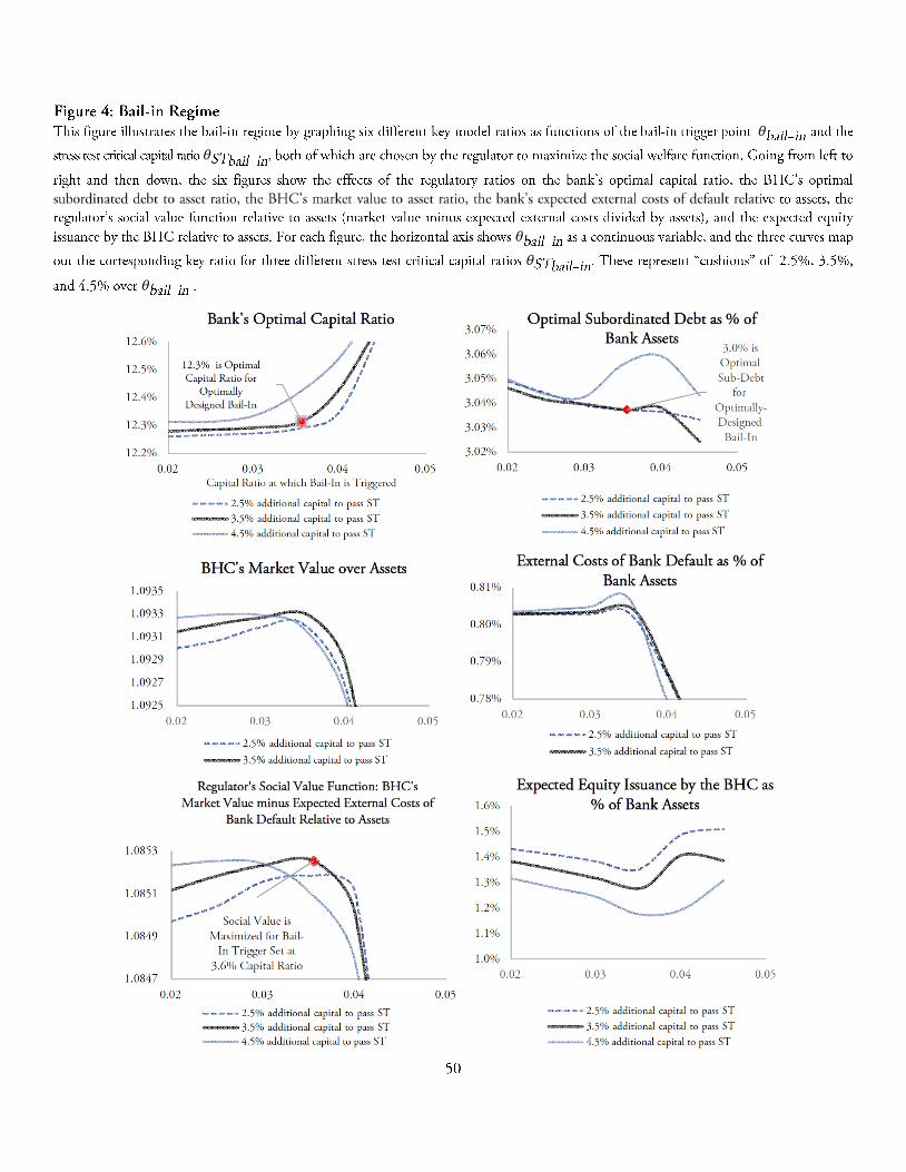
θ

θ

θ

θ

θ

θ

θ

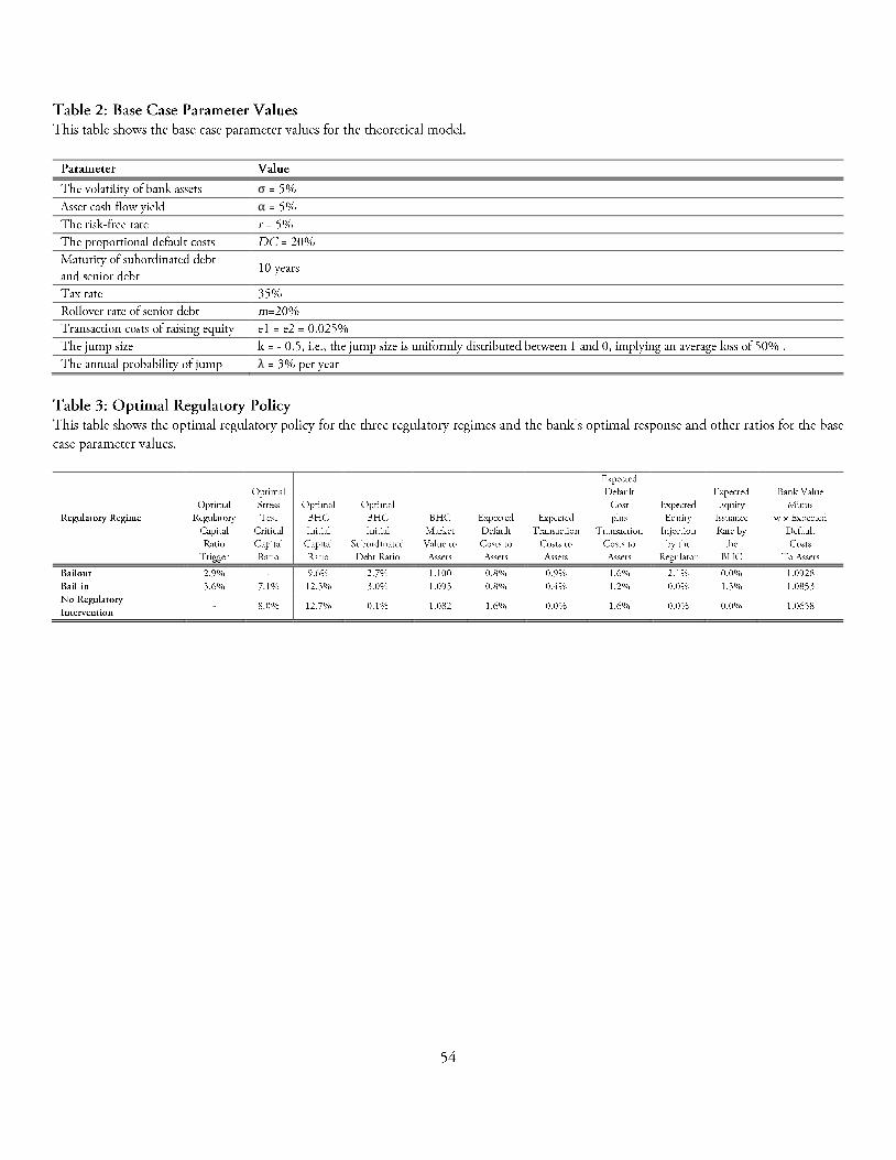
σ

α

λ

×

×

×

×

𝜆

𝜆1 ×

𝜆2 ×

𝜆11 ×

𝜆12 ×

𝜆21 ×

𝜆22 ×

×

𝜆

𝜆1 ×

𝜆2 ×

𝜆11 ×

𝜆12 ×

𝜆21 ×

𝜆22 ×

×

𝜆

𝜆1 ×

𝜆2 ×

𝜆11 ×

𝜆12 ×

𝜆21 ×

𝜆22 ×

×

A Appendix: Analytics of the model

In the following subsections we present the valuation approach of the bank’s equity, senior liabilities, and

subordinated debt for the regime of bail-in. A valuation for bail-out and the ordinary bankruptcy is similar,

expect that some boundary conditions are different.

A.1 Valuation of the bank’s equity for the case with bail-in

In this section, we present valuation of the bank’s equity for the case before bail-in E(V, F +C, t), and after

the bail-in intervention E(V, F, t). The value of equity is a function of its asset value V ; debt principal of

senior and subordinated debt F +C, if no bail-in intervention took place in prior periods, and time t (≤ T ).

First, we describe the valuation of equity for the case in which the bail-in intervention has already taken

place in prior periods. For this case, subordinated debt is converted to equity, and the bank continues paying

interest of its senior debt f and has to pay off its par value F at maturity. At maturity date T , the value of

the bank’s equity is

E(V, F, T ) = max(0, V − F ). (1)

Any time prior to maturity, using standard arbitrage arguments, the value of the equity E(V, F, t) is

given by the solution to the following partial integro-differential equation (PIDE):

σ2V 2

2∂2E∂V 2 + (r − α− λ · k) ∂E∂V + ∂E

∂t + αV − (1− τ) · f

−m · (F −D)− rE − λ · EQt {E(Y · V, F, t)− E(V, F, t)} = 0,

for any V > F ,

(2)

where EQ is the expectation operator under the risk neutral measure Q. In this equation, αV is the

after-tax cash flow generated by the bank’s assets and αV − (1− τ) · f −m · (F −D) is the dividend payout

to the shareholders; and the last term represents the expected change in equity value due to jumps.

If the bank’s capital ratio declines below the minimum capital ratio specified by the stress test, i.e., if

(Vt−F )Vt

< θSTbail−in,then the bank will have to retain all its residual cash flows. As such, the bank has

to reduce its asset payout ratio from α to αST so that it’s dividend payout is zero (or non-positive), i.e.,

αSTVt − (1 − τ)f − m · (F − Dt)) 5 0. Thus, any time t, αSTbail−in = MIN{α, (1−τ)f+m·(F−Dt)Vt

}, if

(Vt−F )Vt

< θSTbail−in, and parameter α is replaced by αSTbail−in in the above equation.

Note that after the subordinated debt converts, the bank will not elect to raise equity capital because

i

such transaction would dilute the shareholders’ value and will benefit holders of the senior debt at the

shareholders’ expense.

Now, consider the valuation of the bank’s equity for the case if the bail-in has not been invoked in the

prior periods. At maturity t = T : E(V, F + C, T ) = V − C − F, if V−FV > θbail−in, and V−F−CV > 0, no bail-in intervention,

E(V, F + C, T ) = 0, if V−FV < θbail−in, or V−F−CV < 0, and V ≥ F .

Prior to maturity, t < T , the bank can choose to raise equity. The choice of equity issuance maximizes the

market value of the bank’s exisitng equity. The solution involves determining free boundary conditions that

divide the state space (V, {F + C }, t) into four regions that characterize the bank’s choices: the no equity

issuance region, the equity issuance region, the bail-in intervention region, and the default region.1

In the no equity issuance region, it is not optimal for the bank to issue new equity capital. In this region,

the equity value E(V, F +C, t) equals the instantaneous cash flow net of coupon payment plus the expected

value of the equity at time t+ ∆t calculated under the risk neutral measure Q:

E(V, F + C, t) = [αV − (1− τ) · (f + c)−m · (F −D)]dt

+ e−rdtEQ{E(Vt+dt, F + C, t+ dt)}, t+ dt ≤ T. (3)

In this region, the equityholders will not choose to issue equity and the following inequalities must hold

for any ∆V :

[αVt − (1− τ) · (f + c)−m · (F −D)]dt+ e−rdtEQ(E(Vt+dt +4V, F + C, t+ dt) )−4V − TC <

αVt − (1− τ) · (f + c)−m · (F −D)]dt+ e−rdtEQ(E(Vt+dt, F + C, t+ dt)),

for any 4V > 0 ,

(4)

i.e., equity issuance is not profitable, where TC are transaction costs of raising equity, TC = e1·Vt+e2·4V .

The value of the equity E(Vt, F+C, t) in the no equity issuance region is given by the solution to the following

PIDE:

1For brevity, we omit the discussion of the technical detail of boundary and “high contact” conditions that applied to thevalue function E. For details see Oksendal and Sulem (2007).

ii

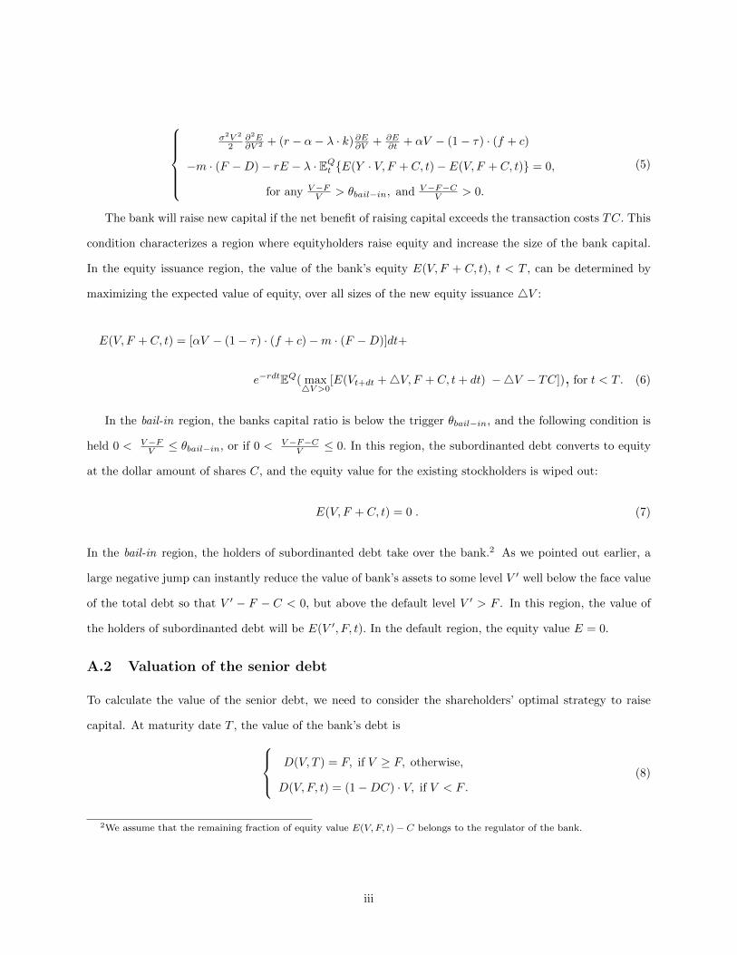
σ2V 2

2∂2E∂V 2 + (r − α− λ · k) ∂E∂V + ∂E

∂t + αV − (1− τ) · (f + c)

−m · (F −D)− rE − λ · EQt {E(Y · V, F + C, t)− E(V, F + C, t)} = 0,

for any V−FV > θbail−in, and V−F−C

V > 0.

(5)

The bank will raise new capital if the net benefit of raising capital exceeds the transaction costs TC. This

condition characterizes a region where equityholders raise equity and increase the size of the bank capital.

In the equity issuance region, the value of the bank’s equity E(V, F + C, t), t < T , can be determined by

maximizing the expected value of equity, over all sizes of the new equity issuance 4V :

E(V, F + C, t) = [αV − (1− τ) · (f + c)−m · (F −D)]dt+

e−rdtEQ( max4V >0

[E(Vt+dt +4V, F + C, t+ dt) −4V − TC]), for t < T . (6)

In the bail-in region, the banks capital ratio is below the trigger θbail−in, and the following condition is

held 0 < V−FV ≤ θbail−in, or if 0 < V−F−C

V ≤ 0. In this region, the subordinanted debt converts to equity

at the dollar amount of shares C, and the equity value for the existing stockholders is wiped out:

E(V, F + C, t) = 0 . (7)

In the bail-in region, the holders of subordinanted debt take over the bank.2 As we pointed out earlier, a

large negative jump can instantly reduce the value of bank’s assets to some level V ′ well below the face value

of the total debt so that V ′ − F − C < 0, but above the default level V ′ > F . In this region, the value of

the holders of subordinanted debt will be E(V ′, F, t). In the default region, the equity value E = 0.

A.2 Valuation of the senior debt

To calculate the value of the senior debt, we need to consider the shareholders’ optimal strategy to raise

capital. At maturity date T , the value of the bank’s debt is D(V, T ) = F, if V ≥ F, otherwise,

D(V, F, t) = (1−DC) · V, if V < F .(8)

2We assume that the remaining fraction of equity value E(V, F, t)− C belongs to the regulator of the bank.

iii

where DC represents proportional default costs (0 ≤ DC ≤ 1). Any time prior to maturity t < T , the value

of debt satisfies:

σ2V 2

2∂2D∂V 2 + (r − α− λ · k)∂D∂V + ∂D

∂t + f +m · (F −D)− rD−

λ · EQt {D(Y · V, F + C, t)−D(V, F + C, t)} = 0,

if E(V, F + C, t) ≥ 0, no prior bail-in intervention

σ2V 2

2∂2D∂V 2 + (r − α− λ · k)∂D∂V + ∂D

∂t + f +m · (F −D)− rD−

λ · EQt {D(Y · V, F, t)−D(V, F, t)} = 0, if the bail-in has taken place in prior periods.

(9)

In the bail-in region, the value of the senior debt is

D(V, F + C, t) = D(V, F, t), if 0 ≤ V − FV

≤ θ, orV − F − C

V≤ 0 and 0 ≤ V − F

V. (10)

In the region where the bank issues equity and increases its capital by 4V , the value of senior debt satisfies:

D(V, F + C, t+) = D(V +4V, F + C, t). (11)

In the default region, the assets are transferred to the holders of the senior debt:

D(V, F, t) = (1−DC) · V . (12)

A.3 Valuation of the subordinated debt

Holders of subordinanted debt have lower priority at default, and for most parameter will recover zero value.

To calculate the value of subordinanted debt, we need to consider the bank’s strategy to raise capital as well

the possibility of bank being bailed-in. At the maturity date T , if the bail-in has not taken place in prior

periods, the value of the subordinated debt, Z(V, F + C, T ) isZ(V, F + C, T ) = C, V−F

V ≥ θbail−in, and 0 < V−F−CV ,

Z(V, F + C, T ) = min{(V − F ), C}, if 0 < V−FV < θ , or 0 < V−F−C

V < 0 and V−FV ≥ θbail−in,

Z(V, F + C, T ) = 0, otherwise.

(13)

Any time prior to maturity t < T , the value of subordinated debt satisfies:

σ2V 2

2∂2Z∂V 2 + (r − α− λ · k) ∂Z∂V + ∂Z

∂t + c− rZ − λ · EQt {Z(Yt · V, F + C, t)− Z(V, F + C, t)} = 0,

if V−FV ≥ θbail−in, and 0 < V−F−CV .

(14)

iv

At the bail-in intervention boundary, the value of the subordinated debt is

Z(V, F + C, t) = min{E(V, F, t), C}, (15)

and the bank remains operational and is taken over by the holders of the subordinated debt.

In the region where the bank issues equity and increases its capital by 4V at t, the value of subordinated

debt satisfies:

Z(V, F + C, t+) = Z(V +4V, F + C, t). (16)

In the default region:

Z(V, F + C, t+) = 0. (17)

v

×

×