Bandwidth–reduced Linear Models of

Non–continuous Power System Components

Jonas Persson

Stockholm 2006Sweden

Doctoral DissertationRoyal Institute of Technology (KTH)

School of Electrical EngineeringElectric Power Systems

ISBN-91-7178-393-8 · TRITA-EE 2006:022 · ISSN-1650-674X

To Eva and Elias

Abstract

This thesis is focused in modelling of power system componentsand their representation in simulations of power systems.

The thesis compares different linearization techniques. These tech-niques are both numerical as well as analytical and are utilized whenlinearization of a dynamic system is desired. After a linearization it ispossible to calculate the eigenvalues of the linearized system as well asto perform other applicable activities on a linear system. In the thesisit is shown how the linearization techniques influence the calculationof eigenvalues of the linear system.

In the thesis bandwidth-reduced linear models of a power systemcomponent are developed using two techniques. The simulations withthe linear models are done with an introduced interface system. Thestudied power system component is a Thyristor-Controlled Series Ca-pacitor (TCSC).

One advantage with using a linear representation of a power systemcomponent is that it simplifies the simulations. The size of the com-plexity of a simulation when solving the equations decreases and theconsumed physical time to simulate becomes shorter. A disadvantageof a linear model is that its validity might be limited.

The need of building linear models of power systems will continueto attract interest in the future. With the horizon of today (year 2006)there is a need of among other models to build linear models of detailedmodels of High Voltage Direct Current-links (HVDC-links), Static VarCompensators (SVCs), as well as Thyristor-Controlled Series Capac-itors (TCSCs). How should these be represented when we want tostudy the dynamics of a whole power system and it is necessary toreduce their complexity? This question rises when we want to performtime-domain simulations with a not too detailed level of complexity ofeach individual power system component or if we want to linearize thepower system and study it within small-signal stability analysis.

v

vi

Sammanfattning

Denna avhandling ar fokuserad pa modellering av elkraftsystem-komponenter och deras representation vid simuleringar av elkraftsys-tem.

Avhandlingen jamfor olika linjariseringstekniker. Dessa tekniker arsaval numeriska som analytiska och anvands vid linjarisering av ettdynamiskt system. Efter en linjarisering ar det mojligt att beraknaegenvardena av det linjariserade systemet samt anvanda andra verk-tyg amnade for studier av linjara system. I avhandlingen visas hur olikalinjariseringtekniker influerar egenvardesberakningen av det linjara sys-temet.

I avhandlingen tas fram bandviddsreducerade linjara modeller aven kraftsystemkomponent med hjalp av tva tekniker. Senare gors simu-leringar med de linjara modellerna tillsammans med ett introduceratgranssnitt. Den studerade kraftsystemkomponenten ar en tyristorstyrdseriekondensator (TCSC).

En fordel med att anvanda en linjar representation av en kraft-systemkomponent ar att det forenklar simuleringarna. Storleken pakomplexiteten av en simulering vid losandet av ekvationerna minskaroch den konsumerade fysiska tiden att simulera minskar. En nackdelmed en linjar modell ar att dess giltighet kan vara begransad.

Behovet av att bygga linjara modeller av kraftsystemkomponentertorde aven finnas i framtiden. Med dagens horisont (ar 2006) finns be-hov av att bygga linjara modeller utgaende fran detaljerade modellerav bl a hogspanda likstromslankar (HVDC-lankar), reaktiva effektkom-pensatorer (SVC) samt tyristorstyrda seriekondensatorer (TCSC). Hurskall dessa representeras nar vi vill studera dynamiken av ett heltkraftsystem och det da ar nodvandigt att reducera deras komplex-itet? Denna fragestallning kommer upp nar vi vill genomfora tids-domansimuleringar pa en inte alltfor detaljerad niva av de individuellakraftsystemkomponenterna eller nar vi vill linjarisera kraftsystemet foratt studera dess stabilitet med hjalp av smasignalanalys.

vii

viii

Table of Contents

Abstract v

Sammanfattning vii

Table of Contents ix

Acknowledgement xxi

1 Introduction 11.1 Background . . . . . . . . . . . . . . . . . . . . . . . . . . . . 11.2 Problem formulation . . . . . . . . . . . . . . . . . . . . . . . 31.3 Main contributions of the thesis . . . . . . . . . . . . . . . . . 41.4 Previous research in the area . . . . . . . . . . . . . . . . . . 51.5 Outline of the thesis . . . . . . . . . . . . . . . . . . . . . . . 51.6 List of publications . . . . . . . . . . . . . . . . . . . . . . . . 5

2 Linearization 92.1 Introduction . . . . . . . . . . . . . . . . . . . . . . . . . . . . 92.2 Background . . . . . . . . . . . . . . . . . . . . . . . . . . . . 102.3 Problem formulation . . . . . . . . . . . . . . . . . . . . . . . 112.4 Linearization methods . . . . . . . . . . . . . . . . . . . . . . 11

2.4.1 Analytical linearization, AL method . . . . . . . . . . 142.4.2 Forward-difference approximation, FDA method . . . 172.4.3 Center-difference approximation, CDA method . . . . 19

2.5 Linearization of a classical machine . . . . . . . . . . . . . . . 202.5.1 Linearization of a classical machine using the AL me-

thod . . . . . . . . . . . . . . . . . . . . . . . . . . . . 242.5.2 Linearization of a classical machine using the FDA

method . . . . . . . . . . . . . . . . . . . . . . . . . . 27

ix

2.5.3 Linearization of a classical machine using the CDAmethod . . . . . . . . . . . . . . . . . . . . . . . . . . 30

2.6 Comparison of the three linearization methods . . . . . . . . 322.6.1 Truncation errors . . . . . . . . . . . . . . . . . . . . . 34

2.7 Large-disturbance stability analysis . . . . . . . . . . . . . . . 362.8 Summary . . . . . . . . . . . . . . . . . . . . . . . . . . . . . 41

3 Modelling the power system in the thesis 433.1 Simulations in instantaneous value mode . . . . . . . . . . . . 43

3.1.1 The dq0 -representation . . . . . . . . . . . . . . . . . 433.2 Per unit system . . . . . . . . . . . . . . . . . . . . . . . . . . 47

3.2.1 Per unit system used in instantaneous value mode . . 483.3 The original model of the Thyristor-Controlled Series Capacitor 49

3.3.1 The structure of the TCSC control . . . . . . . . . . . 523.3.2 Assumptions of the TCSC . . . . . . . . . . . . . . . . 53

3.4 Use of filter to remove harmonics . . . . . . . . . . . . . . . . 603.5 The accuracy of the model of the Thyristor-Controlled Series

Capacitor . . . . . . . . . . . . . . . . . . . . . . . . . . . . . 613.6 Summary . . . . . . . . . . . . . . . . . . . . . . . . . . . . . 61

4 Developing linear models 634.1 Introduction . . . . . . . . . . . . . . . . . . . . . . . . . . . . 634.2 Different methodologies . . . . . . . . . . . . . . . . . . . . . 66

4.2.1 Poincare map . . . . . . . . . . . . . . . . . . . . . . . 664.2.2 Identification from Bode plots . . . . . . . . . . . . . . 664.2.3 Linearised discrete-time model . . . . . . . . . . . . . 674.2.4 Analytical Modelling of TCSC for SSR Studies . . . . 674.2.5 Phasor Dynamics . . . . . . . . . . . . . . . . . . . . . 694.2.6 Prony Analysis . . . . . . . . . . . . . . . . . . . . . . 694.2.7 Discrete-time model . . . . . . . . . . . . . . . . . . . 694.2.8 State-space model depending on the firing angle . . . 704.2.9 Summary of different methodologies . . . . . . . . . . 70

4.3 Introduction to linearization of the TCSC . . . . . . . . . . . 714.4 Investigations of our component . . . . . . . . . . . . . . . . . 74

4.4.1 Isolated perturbations . . . . . . . . . . . . . . . . . . 764.4.2 Simultaneous perturbations . . . . . . . . . . . . . . . 78

4.5 Definition of a linear system . . . . . . . . . . . . . . . . . . . 804.6 Subsystem 12 . . . . . . . . . . . . . . . . . . . . . . . . . . . 814.7 Transient Analysis . . . . . . . . . . . . . . . . . . . . . . . . 86

4.7.1 Preparation of the signals . . . . . . . . . . . . . . . . 87

x

4.7.2 Identification of the four subsystems . . . . . . . . . . 884.7.3 A check of the linear model developed from transient

analysis . . . . . . . . . . . . . . . . . . . . . . . . . . 944.8 Frequency Analysis . . . . . . . . . . . . . . . . . . . . . . . . 94

4.8.1 Anti-aliasing filter . . . . . . . . . . . . . . . . . . . . 974.8.2 Window function . . . . . . . . . . . . . . . . . . . . . 1004.8.3 Identification of the four subsystems . . . . . . . . . . 1014.8.4 A check of the linear model developed from frequency

analysis . . . . . . . . . . . . . . . . . . . . . . . . . . 1044.9 Summary . . . . . . . . . . . . . . . . . . . . . . . . . . . . . 105

5 Interface to a linear model 1075.1 Introduction . . . . . . . . . . . . . . . . . . . . . . . . . . . . 1075.2 Coordinate system . . . . . . . . . . . . . . . . . . . . . . . . 1085.3 Interface system . . . . . . . . . . . . . . . . . . . . . . . . . 109

5.3.1 Phasor estimation . . . . . . . . . . . . . . . . . . . . 1105.3.2 Combined coordinate transformation and filtering . . 1115.3.3 Time constants to filter ISS and Ivar . . . . . . . . . . 1135.3.4 Input signals to the linear model . . . . . . . . . . . . 1145.3.5 Output signals from the linear model . . . . . . . . . . 1165.3.6 Steady-state model . . . . . . . . . . . . . . . . . . . . 116

5.4 Summary . . . . . . . . . . . . . . . . . . . . . . . . . . . . . 117

6 Time-domain simulations 1196.1 Background . . . . . . . . . . . . . . . . . . . . . . . . . . . . 1196.2 Settings of the interface system . . . . . . . . . . . . . . . . . 119

6.2.1 Setting the time constant TF2 in the interface . . . . . 1206.2.2 Setting the time constant TF1 in the interface . . . . . 123

6.3 Description of the test network . . . . . . . . . . . . . . . . . 1246.3.1 Description of the three cases of time-domain simulation125

6.4 Case a . . . . . . . . . . . . . . . . . . . . . . . . . . . . . . . 1276.5 Case b . . . . . . . . . . . . . . . . . . . . . . . . . . . . . . . 1316.6 Case c . . . . . . . . . . . . . . . . . . . . . . . . . . . . . . . 1316.7 Summary . . . . . . . . . . . . . . . . . . . . . . . . . . . . . 134

7 Small-signal stability analysis 1377.1 Background . . . . . . . . . . . . . . . . . . . . . . . . . . . . 1377.2 Studying the two linear models . . . . . . . . . . . . . . . . . 138

7.2.1 Studying the linear model derived from transient anal-ysis . . . . . . . . . . . . . . . . . . . . . . . . . . . . 138

xi

7.2.2 Studying the linear model derived from frequency anal-ysis . . . . . . . . . . . . . . . . . . . . . . . . . . . . 141

7.3 Summary . . . . . . . . . . . . . . . . . . . . . . . . . . . . . 141

8 Summary and conclusions of the thesis 1438.1 Conclusions . . . . . . . . . . . . . . . . . . . . . . . . . . . . 143

8.1.1 Linearization methods . . . . . . . . . . . . . . . . . . 1438.1.2 Bandwidth-reduced linear models of non-continuous

power system components . . . . . . . . . . . . . . . . 1448.2 Possible future work . . . . . . . . . . . . . . . . . . . . . . . 145

A System data for the classical machine 147A.1 System data . . . . . . . . . . . . . . . . . . . . . . . . . . . . 147A.2 Power-flow solution . . . . . . . . . . . . . . . . . . . . . . . . 147A.3 Linearization of example 12.2 in Kundur [35] . . . . . . . . . 149

B Truncation errors for the FDA and CDA methods 151B.1 Truncation error for the FDA method . . . . . . . . . . . . . 151B.2 Truncation error for the CDA method . . . . . . . . . . . . . 155

C Implementation of the TCSC 157C.1 Structure of the TCSC control . . . . . . . . . . . . . . . . . 157C.2 Phase Locked Loop . . . . . . . . . . . . . . . . . . . . . . . . 159C.3 Booster . . . . . . . . . . . . . . . . . . . . . . . . . . . . . . 165C.4 Thyristor Pulse Generator . . . . . . . . . . . . . . . . . . . . 167C.5 Thyristors . . . . . . . . . . . . . . . . . . . . . . . . . . . . . 170C.6 The rhythm of the thyristors . . . . . . . . . . . . . . . . . . 170C.7 Initialization of the TCSC control . . . . . . . . . . . . . . . . 171

C.7.1 Initialization of the Phase Locked Loop, PLL . . . . . 171C.7.2 Initialization of the Booster, BOO . . . . . . . . . . . 171C.7.3 Initialization of the Thyristor Pulse Generator, TPG . 171C.7.4 Initialization of the Thyristors, THY . . . . . . . . . . 171

D Exciter, governor, and turbine models 173D.1 Exciter model . . . . . . . . . . . . . . . . . . . . . . . . . . . 173D.2 Governor model . . . . . . . . . . . . . . . . . . . . . . . . . . 174D.3 Turbine model . . . . . . . . . . . . . . . . . . . . . . . . . . 175

Bibliography 177

xii

List of Figures

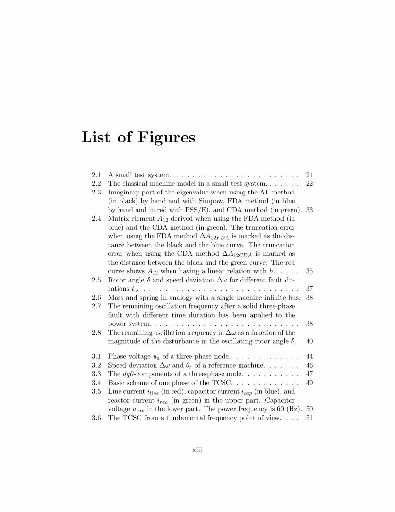
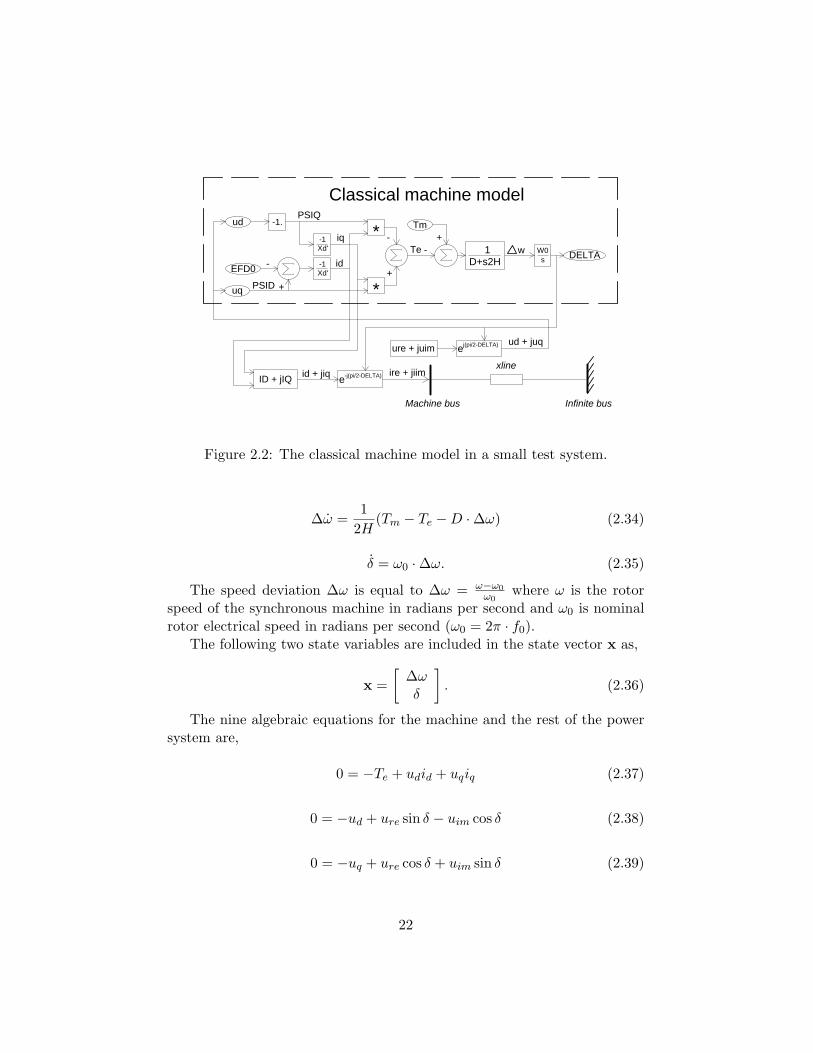
2.1 A small test system. . . . . . . . . . . . . . . . . . . . . . . . 212.2 The classical machine model in a small test system. . . . . . . 222.3 Imaginary part of the eigenvalue when using the AL method

(in black) by hand and with Simpow, FDA method (in blueby hand and in red with PSS/E), and CDA method (in green). 33

2.4 Matrix element A12 derived when using the FDA method (inblue) and the CDA method (in green). The truncation errorwhen using the FDA method ∆A12FDA is marked as the dis-tance between the black and the blue curve. The truncationerror when using the CDA method ∆A12CDA is marked asthe distance between the black and the green curve. The redcurve shows A12 when having a linear relation with h. . . . . 35

2.5 Rotor angle δ and speed deviation ∆ω for different fault du-rations tc. . . . . . . . . . . . . . . . . . . . . . . . . . . . . . 37

2.6 Mass and spring in analogy with a single machine infinite bus. 382.7 The remaining oscillation frequency after a solid three-phase

fault with different time duration has been applied to thepower system. . . . . . . . . . . . . . . . . . . . . . . . . . . . 38

2.8 The remaining oscillation frequency in ∆ω as a function of themagnitude of the disturbance in the oscillating rotor angle δ. 40

3.1 Phase voltage ua of a three-phase node. . . . . . . . . . . . . 443.2 Speed deviation ∆ω and θr of a reference machine. . . . . . . 463.3 The dq0 -components of a three-phase node. . . . . . . . . . . 473.4 Basic scheme of one phase of the TCSC. . . . . . . . . . . . . 493.5 Line current iline (in red), capacitor current icap (in blue), and

reactor current irea (in green) in the upper part. Capacitorvoltage ucap in the lower part. The power frequency is 60 (Hz). 50

3.6 The TCSC from a fundamental frequency point of view. . . . 51

xiii

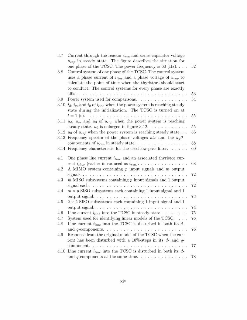
3.7 Current through the reactor irea and series capacitor voltageucap in steady state. The figure describes the situation forone phase of the TCSC. The power frequency is 60 (Hz). . . . 52

3.8 Control system of one phase of the TCSC. The control systemuses a phase current of iline and a phase voltage of ucap tocalculate the point of time when the thyristors should startto conduct. The control systems for every phase are exactlyalike. . . . . . . . . . . . . . . . . . . . . . . . . . . . . . . . . 53

3.9 Power system used for comparisons. . . . . . . . . . . . . . . 543.10 id, iq, and i0 of iline when the power system is reaching steady

state during the initialization. The TCSC is turned on att = 1 (s). . . . . . . . . . . . . . . . . . . . . . . . . . . . . . 55

3.11 ud, uq, and u0 of ucap when the power system is reachingsteady state. u0 is enlarged in figure 3.12. . . . . . . . . . . . 55

3.12 u0 of ucap when the power system is reaching steady state. . . 563.13 Frequency spectra of the phase voltages abc and the dq0 -

components of ucap in steady state. . . . . . . . . . . . . . . . 583.14 Frequency characteristic for the used low-pass filter. . . . . . 60

4.1 One phase line current iline and an associated thyristor cur-rent ithyr (earlier introduced as irea). . . . . . . . . . . . . . . 68

4.2 A MIMO system containing p input signals and m outputsignals. . . . . . . . . . . . . . . . . . . . . . . . . . . . . . . . 72

4.3 m MISO subsystems containing p input signals and 1 outputsignal each. . . . . . . . . . . . . . . . . . . . . . . . . . . . . 72

4.4 m× p SISO subsystems each containing 1 input signal and 1output signal. . . . . . . . . . . . . . . . . . . . . . . . . . . . 73

4.5 2 × 2 SISO subsystems each containing 1 input signal and 1output signal. . . . . . . . . . . . . . . . . . . . . . . . . . . . 74

4.6 Line current iline into the TCSC in steady state. . . . . . . . 754.7 System used for identifying linear models of the TCSC. . . . 764.8 Line current iline into the TCSC is disturbed in both its d -

and q-components. . . . . . . . . . . . . . . . . . . . . . . . . 764.9 Response from the original model of the TCSC when the cur-

rent has been disturbed with a 10%-steps in its d - and q-component. . . . . . . . . . . . . . . . . . . . . . . . . . . . . 77

4.10 Line current iline into the TCSC is disturbed in both its d -and q-components at the same time. . . . . . . . . . . . . . . 78

xiv

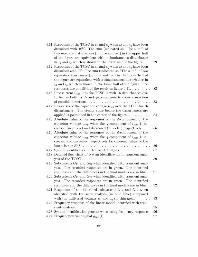
4.11 Responses of the TCSC in ud and uq when id and iq have beendisturbed with 10%. The sum (indicated as ”The sum”) oftwo separate disturbances (in blue and red) in the upper halfof the figure are equivalent with a simultaneous disturbancein id and iq which is shown in the lower half of the figure. . . 79

4.12 Responses of the TCSC in ud and uq when id and iq have beendisturbed with 2%. The sum (indicated as ”The sum”) of twoseparate disturbances (in blue and red) in the upper half ofthe figure are equivalent with a simultaneous disturbance inid and iq which is shown in the lower half of the figure. Theresponses are one fifth of the result in figure 4.11. . . . . . . . 82

4.13 Line current iline into the TCSC is with 16 disturbances dis-turbed in both its d - and q-components to cover a selectionof possible directions. . . . . . . . . . . . . . . . . . . . . . . . 83

4.14 Responses of the capacitor voltage ucap over the TCSC for 16disturbances. The steady state before the disturbances areapplied is positioned in the center of the figure. . . . . . . . . 84

4.15 Absolute value of the responses of the d -component of thecapacitor voltage ucap when the q-component of iline is in-creased (in yellow) and decreased (in violet) respectively. . . . 85

4.16 Absolute value of the responses of the d -component of thecapacitor voltage ucap when the q-component of iline is in-creased and decreased respectively for different values of theboost factor Ref . . . . . . . . . . . . . . . . . . . . . . . . . . 86

4.17 System identification in transient analysis. . . . . . . . . . . . 874.18 Detailed flow chart of system identification in transient anal-

ysis of the TCSC. . . . . . . . . . . . . . . . . . . . . . . . . . 894.19 Subsystems G11 and G21 when identified with transient anal-

ysis. The recorded responses are in green. The identifiedresponses and the differences in the final models are in blue. . 91

4.20 Subsystems G12 and G22 when identified with transient anal-ysis. The recorded responses are in green. The identifiedresponses and the differences in the final models are in blue. . 92

4.21 Responses of the identified subsystems G11 and G21 whenidentified with transient analysis (in bold blue) comparedwith the unfiltered voltages ud and uq (in thin green). . . . . 93

4.22 Frequency response of the linear model identified with tran-sient analysis. . . . . . . . . . . . . . . . . . . . . . . . . . . . 95

4.23 System identification process when using frequency response. 964.24 Frequency-variant signal gdist(t). . . . . . . . . . . . . . . . . 97

xv

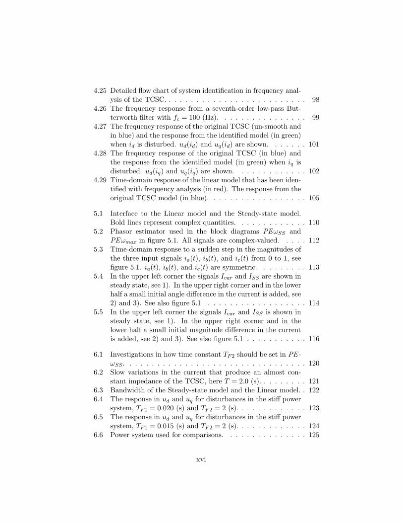
4.25 Detailed flow chart of system identification in frequency anal-ysis of the TCSC. . . . . . . . . . . . . . . . . . . . . . . . . . 98

4.26 The frequency response from a seventh-order low-pass But-terworth filter with fc = 100 (Hz). . . . . . . . . . . . . . . . 99

4.27 The frequency response of the original TCSC (un-smooth andin blue) and the response from the identified model (in green)when id is disturbed. ud(id) and uq(id) are shown. . . . . . . 101

4.28 The frequency response of the original TCSC (in blue) andthe response from the identified model (in green) when iq isdisturbed. ud(iq) and uq(iq) are shown. . . . . . . . . . . . . 102

4.29 Time-domain response of the linear model that has been iden-tified with frequency analysis (in red). The response from theoriginal TCSC model (in blue). . . . . . . . . . . . . . . . . . 105

5.1 Interface to the Linear model and the Steady-state model.Bold lines represent complex quantities. . . . . . . . . . . . . 110

5.2 Phasor estimator used in the block diagrams PEωSS andPEωmax in figure 5.1. All signals are complex-valued. . . . . 112

5.3 Time-domain response to a sudden step in the magnitudes ofthe three input signals ia(t), ib(t), and ic(t) from 0 to 1, seefigure 5.1. ia(t), ib(t), and ic(t) are symmetric. . . . . . . . . 113

5.4 In the upper left corner the signals Ivar and ISS are shown insteady state, see 1). In the upper right corner and in the lowerhalf a small initial angle difference in the current is added, see2) and 3). See also figure 5.1 . . . . . . . . . . . . . . . . . . 114

5.5 In the upper left corner the signals Ivar and ISS is shown insteady state, see 1). In the upper right corner and in thelower half a small initial magnitude difference in the currentis added, see 2) and 3). See also figure 5.1 . . . . . . . . . . . 116

6.1 Investigations in how time constant TF2 should be set in PE -ωSS . . . . . . . . . . . . . . . . . . . . . . . . . . . . . . . . . 120

6.2 Slow variations in the current that produce an almost con-stant impedance of the TCSC, here T = 2.0 (s). . . . . . . . . 121

6.3 Bandwidth of the Steady-state model and the Linear model. . 1226.4 The response in ud and uq for disturbances in the stiff power

system, TF1 = 0.020 (s) and TF2 = 2 (s). . . . . . . . . . . . . 1236.5 The response in ud and uq for disturbances in the stiff power

system, TF1 = 0.015 (s) and TF2 = 2 (s). . . . . . . . . . . . . 1246.6 Power system used for comparisons. . . . . . . . . . . . . . . 125

xvi

6.7 The power system wherein the TCSC is modelled with a linearmodel M(s) including an interface system. . . . . . . . . . . . 126

6.8 id, iq, ud, and uq for the original TCSC model in case a. . . . 1286.9 The currents id and iq through the TCSC from figure 6.8

depicted in one diagram, case a. . . . . . . . . . . . . . . . . . 1286.10 Real and reactive power through the TCSC into node B, case

a. . . . . . . . . . . . . . . . . . . . . . . . . . . . . . . . . . . 1296.11 id, iq, ud, and uq for the original TCSC model (in blue) and

the Steady-state model (in black) in case a. . . . . . . . . . . 1296.12 id, iq, ud, and uq for the original TCSC model (in blue), the

linear model identified from Transient Analysis (in black),and the linear model identified from Frequency Analysis (inred) in case a. . . . . . . . . . . . . . . . . . . . . . . . . . . . 130

6.13 Focused picture of ud and uq for the original TCSC model(in blue), the linear model identified from Transient Analysis(in black), and the linear model identified from FrequencyAnalysis (in red) in case a. . . . . . . . . . . . . . . . . . . . . 130

6.14 id, iq, ud, and uq for the original TCSC model (in blue), thelinear model identified from Transient Analysis (in black),and the linear model identified from Frequency Analysis (inred) in case b. . . . . . . . . . . . . . . . . . . . . . . . . . . . 132

6.15 Focused picture of ud and uq for the original TCSC model(in blue), the linear model identified from Transient Analysis(in black), and the linear model identified from FrequencyAnalysis (in red) in case b. . . . . . . . . . . . . . . . . . . . . 132

6.16 id, iq, ud, and uq for the original TCSC model (in blue), thelinear model identified from Transient Analysis (in black),and the linear model identified from Frequency Analysis (inred) in case c. . . . . . . . . . . . . . . . . . . . . . . . . . . . 133

6.17 Focused picture of ud and uq for the original TCSC model(in blue), the linear model identified from Transient Analysis(in black), and the linear model identified from FrequencyAnalysis (in red) in case c. . . . . . . . . . . . . . . . . . . . . 133

7.1 The power system wherein the TCSC is modelled with M(s)containing a steady-state model, a linear model as well as aninterface system. . . . . . . . . . . . . . . . . . . . . . . . . . 139

7.2 Interface to the Linear model and the Steady-state model.Bold lines represent complex quantities. . . . . . . . . . . . . 139

xvii

A.1 The classical machine model in a small test system. . . . . . . 148

C.1 Basic scheme of the Thyristor-Controlled Series Capacitor(TCSC). . . . . . . . . . . . . . . . . . . . . . . . . . . . . . . 158

C.2 Control system of one phase of the TCSC. The control sys-tem uses a phase current iline and a phase voltage over theseries capacitor ucap to calculate the point of time when thethyristors should start to conduct. The control systems forall phases are exactly alike. . . . . . . . . . . . . . . . . . . . 158

C.3 The upper part shows one phase current of iline and the lowerpart shows TetaPLL. TetaPLL is synchronized so that it is0 when iline reaches its maximum, see t = 5.03 (s). TetaPLLis varying in the interval −π

2 ≤ TetaPLL < 3π2 . . . . . . . . . 161

C.4 Block diagram of the PLL. . . . . . . . . . . . . . . . . . . . . 162C.5 The upper part shows that the value of TetaPLL sets Count-

Rev and CountFor. When CountRev = 1 the value ofTimeRev is calculated and when CountFor = 1 the value ofTimeFor is calculated, see the middle part of the figure. Thelower part of the figure shows that TimeRev and TimeForare predicted time points for next occurring minimum, see A1

and A2, and maximum, see B1 and B2 for the reactor currentirea. . . . . . . . . . . . . . . . . . . . . . . . . . . . . . . . . 163

C.6 The series capacitor voltage ucap and the current through thereactor irea in steady state. The figure describes the situationfor one phase of the TCSC. . . . . . . . . . . . . . . . . . . . 164

C.7 Block diagram of the BOO. . . . . . . . . . . . . . . . . . . . 166C.8 Block diagram of the TPG. . . . . . . . . . . . . . . . . . . . 169C.9 A block diagram inside the TPG containing an implicit equa-

tion when solving BF . . . . . . . . . . . . . . . . . . . . . . . 169

D.1 Block diagram of excitation system with DC commutator ex-citer (IEEE Type = DC1) of S1 and S2. . . . . . . . . . . . . 174

D.2 Block diagram of the governors for S1 and S2. . . . . . . . . . 174D.3 Block diagram of the steam turbines for S1 and S2. . . . . . . 175

xviii

List of Tables

2.1 Settings of the classical machine model in section 2.5. . . . . 212.2 Eigenvalues of the classical machine in subsections 2.5.1 –

2.5.3. The eigenvalue’s real and imaginary parts are given in[1/s] and [rad/s] respectively. All results are calculated byhand. . . . . . . . . . . . . . . . . . . . . . . . . . . . . . . . 32

3.1 Harmonics in the three-phase voltages of ucap (abc-components)of the TCSC and how they appear in the dq0 -components. . 59

4.1 Complex poles for Kayenta System, see Jalali [26]. . . . . . . 674.2 Frequencies used to disturb the TCSC. . . . . . . . . . . . . . 96

6.1 Maximum difference in reactance in figure 6.1. . . . . . . . . 121

7.1 Complex poles with real part greater than −200 with thelinear model identified from transient analysis. Eigenvaluesλ1 – λ14 are found in phasor mode when the TCSC is modelledas a constant series capacitor. . . . . . . . . . . . . . . . . . . 140

7.2 Complex poles with real part greater than -200 with the linearmodel identified from frequency analysis. Eigenvalues λ1 –λ14 are found in phasor mode when the TCSC is modelled asa constant series capacitor. . . . . . . . . . . . . . . . . . . . 142

A.1 Settings of the classical machine model in section 2.5. . . . . 147A.2 Power-flow results of the classical machine model in section 2.5.148

C.1 Input parameters to the TCSC system. . . . . . . . . . . . . . 160C.2 The order of the thyristor switches. . . . . . . . . . . . . . . . 170

D.1 Data for exciter model shown in figure D.1. . . . . . . . . . . 173D.2 Data for governor model shown in figure D.2. . . . . . . . . . 174D.3 Data for turbine model shown in figure D.3. . . . . . . . . . . 175

xix

xx

Acknowledgement

This report completes the work carried out since December 1998 at ElectricPower Systems, department of Electrical Engineering, Royal Institute ofTechnology, Stockholm, Sweden, and constitutes my doctorate thesis.

First of all, I want to thank my supervisor, Professor Lennart Soder atthe Royal Institute of Technology, for his advice, support and encourage-ment during the project. I am grateful for his will of finishing this projectby inviting me to a last call during January, 2006. I want to thank Profes-sor Goran Andersson who was my supervisor the first one and a half yearof the project and who invited me to start this project before he left forElectric Power Systems Group, ETH-Zentrum, Zurich, Switzerland. Evenafter Goran left we have continued the contact in many ways which has feltvery stimulating.

I would like to thank the members of the reference group for alwaysdiscussing and supporting the project thoroughly in our meetings: Dr. KjellAneros at STRI, Dr. Bertil Berggren at Corporate Research within ABB,Magnus Danielsson at Svenska Kraftnat, Dr. Mehrdad Ghandhari at theRoyal Institute of Technology, Tech. Lic. Kerstin Linden at STRI, andDr. Sture Torseng and Dr. Lennart Angquist at ABB Power Technologies,Power Systems FACTS.

I want to thank my inspiring former colleagues at ABB Power Tech-nologies, Power Systems FACTS that I have had the opportunity to workwith during my years at ABB and to whom I have been able to ask any-thing I have thought about. They are: Ture Adielson, Dr. Kjell Aneros,Eva Fredricson-Sjogren, Anders Frost, Jean-Philippe Hasler, Bertil Klerfors,Dr. David Larsson, Lars Lindquist, Bengt Lundin, Tech. Lic. Ann Palesjo,Jytte Pedersen, Tore Petersson, Bo Poulsen, Sune Sarri, Sten Stenemar,Tech. Lic. Inger Segerqvist, Ricardo Tenorio, and Dr. Sture Torseng. Myone-or-two-day-a-week in Vasteras has always been a highlight for me. Es-pecially Sture I would like to thank for allowing me to start this industrialcorporation project between ABB and the Royal Institute of Technology.

xxi

I want to thank my new inspiring colleagues at STRI that I have theopportunity to work with. They are: Dr. Kjell Aneros, Professor MathBollen, Ronnie Braner, Tech. Lic. Bengt Franken, Mats Hager, Goran Lin-dahl, Tech. Lic. Kerstin Linden, Lars Lindquist, Lena Lore, Sune Sarri,Magnus Speychal, Tech. Lic. Henrik Stomberg, and Mikael Strom.

One extra thanks goes to Lars Lindquist at STRI for all anytime-Simpow-support, to Dr. Lennart Angquist at ABB Power Technologies, Power Sys-tems FACTS for instructing me in the TCSC model that was used in thethesis and to all his suggestions and support and to Tore Petersson, for-merly at ABB Power Technologies, Power Systems FACTS, for sharing allhis knowledge.

I would like to thank the current and former staff of the group Elec-tric Power Systems at the Royal Institute of Technology for providing thestimulating atmosphere. Special thanks to my roommates: the mathemati-cian Dr. Valery Knyazkin and Tech. Lic. Magnus Ohrstrom, the computerexperts Dr. Erik Thunberg (– I guess you are all specialists...) and Pe-ter Lonn, Dr. Thomas Ackermann, Dr. Mikael Amelin for unforgettablelate night sessions and inspiration when so was needed, Dr. Peter Ben-nich, Dr. Lina Bertling, Elin Brostrom, Tech. Lic. Paulo Fischer de Toledo,Dr. Mehrdad Ghandhari, Dr. Ying He, Dr. Arnim Herbig, Lillemor Hyl-lengren, Ingemar Jonasson for music discussions, Mikael Kronman, ElinLindgren, Tech. Lic. Magnus Lommerdal, Tech. Lic. Julija Matevosyan,Dr. Viktoria Neimane, Dr. Marcio M. de Oliveira, Tech. Lic. Magnus Ols-son, Dr. Niclas Schonborg, Tech. Lic. Torbjorn Solver, Margaretha Surjadi,Peter Svahn, and Tech. Lic. Anders Wikstrom.

The master thesis students I have had the opportunity to meet besidemy project I also want to thank: Erik Ek at Svenska Kraftnat, Anna Eriks-son at Bombardier Transportation, Eva Centeno Lopez at the Swedish En-ergy Agency, Iris Baldursdottir at ABB Power Technologies, Power SystemsFACTS, Emil Johansson at ABB Power Technologies, Francesco Sulla for-merly at ABB Power Technologies, Power Systems FACTS, Abram Perdanaat Chalmers University of Technology, Hanna Jansson and Huda Yasef for-merly at ABB Power Technologies, Power Systems FACTS, and FlorentMaupas formerly at the Royal Institute of Technology.

The under-graduate students I have met when teaching in the coursesat the university is one of the flavors of academic work that I have trulyenjoyed throughout the years. To the group behind the course Electric PowerSystems (Eleffektsystem in Swedish) goes one extra thank you. It has beeninspiring to teach together with you Tech. Lic. Mats Leksell, Professor Hans-Peter Nee, Dr. Bjorn Allebrand, Dr. Freddy Magnussen, Tommy Kjellqvist,

xxii

Dr. Fredrik Carlsson, and Professor Lennart Soder.Through my contacts with Simpow I want to thank all the users that I

have had contact with through support cases, marketing, and user coursesfrom Scandinavia mainly but also from China, India, Malaysia, and Turkey.You have inspired and taught me by describing all kinds of electric phe-nomena you want to simulate and have support to. Special thanks toDr. Bora Alboyaci, Luigi Busarello, Somnath Chakraborty, Giatgen Cott,Steinar Danielsen, Turhan Demiray, Christoph Fischer, Frode Johannessen,Dr. Mattias Jonsson, Dr. Markus Leuzinger, Dr. Tina Orfanogianni, Pro-fessor Alex Petroianu, S Satyanarayan, Roald Sporild, Dr. Kailash Srivas-tava, Oskar Samfors, Dr. Torbjorn Thiringer, Trond Toftevaag, Dr. Wilbur-WeiGuo Wang, Aidong Xu, Dr. Chengyan Yue, and Dr. Changchun Zhou.

I also want to thank Professor Sigurd Skogestad for his fast replies tomy questions regarding MIMO systems.

During half a year in 2002 I was studying at Instituto de InvestigacionTecnologica, IIT, Universidad Pontificia Comillas, Madrid, Spain, with Pro-fessor Luis Rouco as my supervisor. – Thank you Luis for accepting me as aguest to your group de planta dos en IIT. I also want to thank the personnelat IIT for trying to understand my Spanish during the coffee breaks. It wasvery inspiring for me to be with you.

I want to thank ABB, Elforsk, STRI, Svenska Kraftnat, Swedish EnergyAgency, and the Swedish Research Council for providing funding for thisproject.

Finally, I would like to thank those closest to me: My lovely wife Eva,for all her love, support, hugs, cooking, spell-checking of the thesis, andalways understanding. The last year(s) have been hard for us to get thisthesis finished/out of the house but now I hope we can recover when thewriting has been finished. With the birth of Elias our life will now containnew moments. My wonderful parents Hasse and Ingrid I want to thank fortheir love and believing in me and for always giving me permission to dowhatever I have wanted. My sister Ewa with her family Glenn, Alexander,and Rebecca for all love and support. My family in Spain that has supportedme in all possible ways by for instance providing such an inspiring Spanishoffice when finishing this project; Pablo and Mary (Pablo, un doctor deverdad), Pablo and Ana (Pablo for doubts and joyful sudden power systemunderstandings!), Cesar, Marisol, Alvaro and little Silvia.

My friends I would like to thank, among others; Mattias Adomat, ThomasArlevall and Pernilla Frantzich, Christina Chi and Martin Hultquist, SoniaDıez Santos, Anna Flintberg and Olle Asbrink, Esther Garcıa Tomas andElıas Gonzalo Gomez (esta publicacion es un resultado de muchos cafes

xxiii

de Elıas), Manuel Garcıa Hernandez, Anna Granberg, Dr. Hjalmar Gran-berg, Henrik Hermansson and Kristina Andersson, Lance Lindquist, Mat-tias Ludvigsson and Melisa Nielsen, Gonzalo Morgade Rodrıguez and San-dra Rodrıguez Vila, Txus Reyes Revuelta and Irantzu Macua Biurrun, KlasSjoberg and Anna-Mia Johansson, Magnus Sjogren and Sara Sjogren, NiklasSkeri and Carina Skeri, Jose Tejada Fernandez, Sami Zinad and Dr. PetraWillquist.

My last acknowledgement goes to two teachers I have had during mysenior high school and university who have meant a lot to me. They are LarsSamuelsson at Sven Erikson senior high school in Boras, Sweden, teachingmathematics and physics and Sven-Olof Svensson at Malardalen Universityin Ludvika, Sweden, teaching mathematics. I hope I can inspire someone inthe same way as your beautiful teaching in mathematics and physics inspiredme.

Now I hope I will have more time for my family and friends and hopefullyfocus on another stage in my life.

Jonas Persson, Solna, a wonderful sunny day, May, 2006.

xxiv

Chapter 1

Introduction

1.1 Background

Simulation of power systems has been an area of interest since decades.Simulation programs are used to study future alternative solutions in powersystems or to analyze scenarios that have already occurred in order to un-derstand how it is possible to avoid them in the future.

When performing power system studies it is necessary to have appro-priate models. With this means that the models should be on an enoughdetailed level to describe necessary behaviour of a power system componentto match the aim of the study or the simulation.

Today power systems are often driven closer to their limits and duringsuch circumstances knowledge of the systems are even more necessary. Dur-ing recent years some blackouts of power systems have happened partly asconsequences of lacking knowledge of the dynamics of the power system. Af-ter events like blackouts, system operators are analyzing the reason for theblackout and during such analysis even simulation models of components inthe power system have been upgraded since it has been shown that theyhave behaved different during power failures compared to what simulationsof the power system have shown, see for instance Recommendation 24 inU. S.-Canada Power System Outage Task Force [84].

This thesis is focused on representation of complex power system compo-nents in simulations of power systems. Complex power system componentsare technically advanced equipment that make them computationally heavyto simulate. The aim of the project is to neglect the complexity of detailedmodels of components and to build simplified linear models which are stillaccurate but easier to simulate. The linear models are in the thesis investi-

1

gated and compared with the detailed models.In the thesis we are studying a power system component within the

group of Flexible AC Transmission Systems (FACTS) components. We haveselected the Thyristor-Controlled Series Capacitor (TCSC) as our studyobject.

As the title Bandwidth–reduced Linear Models of Non–continuous PowerSystem Components of the thesis is formulated we want to emphasize on thatwe here develop linear models that have a reduced bandwidth. In the thesiswe have focused on fundamental low-frequency behaviour of a power systemcomponent and therefore excluded the representation of higher frequencies.The bandwidth can be expanded to also include higher frequencies, however,the here developed linear models exclude the possibility to study higher fre-quencies like e.g. subsynchronous resonance (SSR) of a power system includ-ing a Thyristor-Controlled Series Capacitor (TCSC).

In the title of the thesis we have used the word non-continuous whichmeans that we analyze models that are in a class of components that sud-denly change setup of differential equations at some certain events. Theseevents are non-continuous. Another word to describe non-continuous (ornot continuous) is discontinuous. In the components we study we have vari-ables that contain ”breaks” at specific time points as described in Gill [18],pp. 46-47.

The differential equations that the studied components contain are alsonon-linear which makes the components non-linear. Normally there is anumber of non-linear models in a power system where a synchronous machineis one example. However, a synchronous machine is modelled with the sameset of differential equations during a simulation. This is opposite with themodels we mean with non-continuous which are suddenly changing setup ofdifferential equations.

The studied component in the project is a Thyristor-Controlled SeriesCapacitor (TCSC) which contains thyristor switchings which are computa-tionally heavy to simulate since they create several events in each period ofthe power system frequency. In the simplified linear models we do not modeleach event (as e.g. a thyristor switch) during a time-domain simulation, likehigh-frequent changes of signals. Instead, the aim is to find linear modelsthat describe the behavior of the non-linear power system component withina certain bandwidth (in our case the TCSC). We are interested in investi-gating the behaviour of the TCSC based on a detailed level of modellingand from that build a linear model containing the behavior within a certainbandwidth of the TCSC.

When the linear models once have been developed they do simplify and

2

speed up time-domain simulations.To make investigations through small-signal stability analysis of a power

system containing non-linear components which during normal conditions(such as a steady state) is periodically changing working point, can be donemore adequately if such components are replaced by linear models.

An interface system has been developed in the thesis project. It connectsthe linear models to the rest of the power system by transforming currentsand voltages between the coordinate system of the network and the localcoordinate system of the linearized component. The interface system canbe actual for use also in other applications of modelling of power systemcomponents.

Since the thesis is focused on linear models, an extensive part of the thesisis discussing linearization of dynamic systems applied to power systems.Three linearization methods are investigated and compared and it is shownhow these methods influence the result obtained from linearizations. Apractical consequence is that three engineers working in parallel, studyingthe same power system but using three different linearization routines, willget different results.

1.2 Problem formulation

When simulating dynamic behavior of power systems it is necessary to havemodels that represent the real components as close as possible, and that theresults correspond to what would also appear in the real power system. Toget simulated results as close as possible to the real power system demandsthe following,

1. Models of the power system components that have enough accuracydepending on the aim of the simulation.

2. A simulator which,

a) accurately solves the power system simulation including solutionof differential and algebraic equations in time-domain simula-tions, i.e., accurate numerical methods, as well as a time step inthe simulation which is set short enough to enable the demandedlevel of accuracy of the study. With accuracy is here meant bothin time resolution as well as the tolerances with which the valuesof the variables are calculated; and

3

b) accurately linearize the power system when performing small-signal stability analysis (linear analysis). Here different toolsshould be included to enable small-signal stability analysis.

3. Accurate information of all components’ parameter values.

Point 2 in the list above can be expanded with more subpoints. However,within the work of this thesis subpoints a and b are the most important.

This thesis deals with points 1 and 2b in the list above.In point 1 the thesis elaborates on the possibility to; from a detailed

model create simpler linear models and compare the performance with theoriginal model and investigate their accuracy. Here it should also be men-tioned that often the following relation appear; the higher level of detail asimulation is performed with, the longer time it takes to simulate.

In point 2b the thesis compares three linearization methods.The power system simulations in the thesis are made with STRI’s power

system simulation software Simpow version 10.2.078, see Fankhauser [16]and [75]. When building linear models, functions of the System IdentificationToolbox provided by Matlab version 6.5.1 is used, see Ljung [41]. AlsoSiemens’ power system simulation software PSS/E version 26, see [67], isused when comparing linearization methods between different software. Thisthesis is written in LATEX.

1.3 Main contributions of the thesis

The main contributions of the thesis are:

• Analysis of how three different linearization methods influence thelinearization of a power system when performing small-signal stabilityanalysis (linear analysis). The linearized power system is later usedwhen studying the locations of the eigenvalues of the power system.

• Use of two methods (Transient Analysis and Frequency Analysis) todevelop linear models of a non-linear power system component. Thetwo methods have been applied in the thesis to create linear modelsof a Thyristor-Controlled Series Capacitor (TCSC).

• Development of an interface system connecting the linear models tothe rest of the power system.

4

• Application and analysis of the created linear models of a TCSC intime-domain simulations in instantaneous value mode of the powersystem.

• Application and analysis of the created linear models of a TCSC insmall-signal stability analysis (linear analysis).

• Evaluation of the developed linear models.

1.4 Previous research in the area

The contributions in what other have done in related works to this thesiscan be found in sections 2.2 and 4.2.

1.5 Outline of the thesis

The outline of the thesis is as follows. Chapter 2 contains a backgroundof linearization and describes three techniques in how to linearize a powersystem.

Chapter 3 describes the modelling of the power system in the thesis anddetails about the modelling of the TCSC. Chapter 4 describes the devel-opment of the linear models and the linearity of the original TCSC model.Chapter 5 introduces the interface system between the identified linear mod-els and the surrounding power system.

Chapter 6 contains comparisons in time-domain simulations and chapter7 compare linearizations of the power system including the linear models ofthe TCSC.

Chapter 8 contains a summary and makes conclusions of the thesis.

1.6 List of publications

The work during the project has been described in the following publications.The material presented in chapter 5 is not yet published in any publication.

Conference papers

[57] Jonas Persson, Kjell Aneros, Jean-Philippe Hasler, Switching a LargePower System Between Fundamental Frequency and Instantaneous Va-lue Mode, in Proceedings of the 3rd International Conference on DigitalPower System Simulators, ICDS’99, Vasteras, Sweden, May 25th –28th, 1999.

5

[61] Jonas Persson, Lennart Soder, Linear Analysis of a Two-Area Sys-tem Including a Linear Model of a Thyristor-Controlled Series Capac-itor, in Proceedings of the IEEE Porto Power Tech Conference 2001,PPT’01, Paper 289, Porto, Portugal, September 10th – 13th, 2001.

[28] Emil Johansson, Jonas Persson, Lars Lindkvist, Lennart Soder, Lo-cation of Eigenvalues Influenced by Different Models of SynchronousMachines, in Proceedings of the 6th IASTED International Multi-Con-ference on Power and Energy Systems, Paper 352–145, Marina del Rey,Los Angeles, USA, May 13th – 15th, 2002.

[78] Han Slootweg, Jonas Persson, A.M. van Voorden, G.C. Paap, WilKling, A Study of the Eigenvalue Analysis Capabilities of Power Sys-tem Dynamics Simulation Software, in Proceedings of the 14th PowerSystems Computation Conference 2002, PSCC’02, Paper 26–3, Sevilla,Spain, June 24th – 28th, 2002.

[62] Jonas Persson, Lennart Soder, Validity of a Linear Model of a Thyr-istor-Controlled Series Capacitor for Dynamic Simulations, in Pro-ceedings of the 14th Power Systems Computation Conference 2002,PSCC’02, Paper 26–6, Sevilla, Spain, June 24th – 28th, 2002.

[60] Jonas Persson, Han Slootweg, Luis Rouco, Lennart Soder, Wil Kling,A Comparison of Eigenvalues Obtained with Two Dynamic SimulationSoftware Packages, in Proceedings of the IEEE Bologna Power TechConference 2003, BPT’03, Paper 254, Bologna, Italy, June 23rd –26th, 2003.

[58] Jonas Persson, Luis Rouco, Lennart Soder, Linear Analysis with TwoLinear Models of a Thyristor-Controlled Series Capacitor, in Proceed-ings of the IEEE Bologna Power Tech Conference 2003, BPT’03, Pa-per 496, Bologna, Italy, June 23rd – 26th, 2003.

[59] Jonas Persson, Luis Rouco, Lennart Soder, Time-Domain Compar-isons of Two Linear Models of a Thyristor-Controlled Series Capaci-tor, in Proceedings of the 6th International Power Engineering Confer-ence, IPEC’03, Paper 1046, Singapore, November 27th – 29th, 2003.

Technical reports

[52] Jonas Persson, Are there any Limits in Building Small-Signal Modelsof Dynamic Systems?, Internal Report, Department of Electric Power

6

Engineering, Electric Power Systems, Royal Institute of Technology,Stockholm, Sweden, 1999.

[56] Jonas Persson, On Linearization of Non-linear Components, A–EES–0014, Internal Report, Department of Electric Power Engineering,Electric Power Systems, Royal Institute of Technology, Stockholm,Sweden, 2000.

[51] Jonas Persson, A description of the Masta model of the Thyristor-Controlled Series Capacitor in Simpow, Technical Report, TR H 00–163A, ABB Power Systems, Vasteras, Sweden, October 12, 2000.

[54] Jonas Persson, How linearization is made in a small power system witha classical representation of a synchronous machine, Internal Report,Department of Electrical Engineering, Electric Power Systems, RoyalInstitute of Technology, Stockholm, Sweden, 2002.

Licentiate thesis

[55] Jonas Persson, Linear Models of Non-linear Power System Compo-nents, Licentiate Thesis, TRITA–ETS–2001–04, ISSN 1650–674X, De-partment of Electrical Engineering, Electric Power Systems, Royal In-stitute of Technology, Stockholm, Sweden, 2002.

Conference papers [28, 78, 60] and the technical report [54] are included inchapter 2. Conference paper [57] and the technical report [51] are includedin chapter 3 and appendix C. Chapter 5 and 6 contain new material that hasnot been published yet. Conference papers [62, 59] are included in chapter6. Conference papers [61, 58] are included in chapter 7.

7

8

Chapter 2

Linearization

In this chapter different methods to linearize a dynamic system are studied,both generally as well as specifically for power systems.

2.1 Introduction

Linearization of a power system is necessary to perform if its small-signalstability should be examined. Small-signal stability of a power system is theability of the power system to maintain in synchronism when subjected tosmall disturbances. In this context, a disturbance is considered to be smallif the equations that describe the resulting response of the system may belinearized for the purpose of the analysis, Kundur [35]. See Kundur [36] fordefinitions of different types of power system stability.

To be able to linearize the system, a linearization method has to beutilized. In this chapter three such linearization methods are documentedand compared. Also two software which use two of the linearization meth-ods are compared and evaluated. It is shown and also explained in whichway the linearization methods influence the results, i.e., the location (thereal and imaginary parts) of the obtained eigenvalues in the complex plane.The conclusions drawn from eigenvalue analysis are thus not only dependenton the properties of the investigated system, but also on which linearizationmethod that is used since software packages use different linearization meth-ods. Therefore, conclusions can differ when studying the same power systemwith different software packages.

9

2.2 Background

Eigenvalues of a power system give a picture of the stability in the currentoperating point. The eigenvalues are calculated from the system matrixof a dynamic system which is here referred to as the A-matrix. To createthe A-matrix, the dynamic system has to be linearized and to do that,linearization methods are utilized when performing small-signal stabilityanalysis of dynamic systems. A power system is one example of a dynamicsystem.

In this chapter differences between three linearization methods are ana-lyzed as well as consequences thereof.

In the chapter all linearizations and simulations are made when sim-ulating in fundamental frequency mode. The models of the power systemcomponents are identical when evaluating the linearization methods. It thenbecomes easier to see the pure influence of the linearization methods.

Calculations are done by hand for the three linearization methods aswell as with two power system simulation software which use two of the lin-earization methods. These are Siemens’ PSS/E [67] and STRI’s Simpow [75].Software that can be used for this purpose can be found in Paserba [50].

In different software, models of the same power system component differ.This is one reason why there are different results when studying eigenvaluesin small-signal stability with different software. However, such comparisonof different models is not done here. In this chapter the models of the powersystem components are identical in all linearizations and software.

Related works where linearization routines are discussed is Martins [43]where the first linearization method below, namely the analytical lineariza-tion method, is utilized. The second method, the forward-difference approx-imation method is a numerical method which can be found in for instanceGill [18]. In Taylor [81] the numerical method center-difference approxima-tion is utilized and it is shown how it is used for a special software. Also thetruncation error is discussed in Taylor [81]. In works of Kaberere [30, 31]comparisons are made with different software for small-signal stability anal-ysis.

In the literature there has not yet been any systematic comparison ofthese three methods applied to power systems.

10

2.3 Problem formulation

There are several software packages on the market that can extract eigen-values, see Paserba [50]. However, the various software are seldom evaluatedand compared. Since the software packages both use different linearizationmethods as well as different models of the power system components it isimportant to understand that the consequence thereof is that there are dif-ferences in the extraction of the eigenvalues between the software packages.

Differences between models which represent a power system componentbut in different software is a source which produces differences when small-signal stability analysis is performed in software. There are numerous ofdifferent synchronous machine models reported in the literature such asKundur [35], Buhler [5], Laible [38], and Canay [6]. Investigations in findingdifferences between machine models can be found in Kundur [35], Johans-son [28], Persson [60], and Slootweg [78] where differences in representationof synchronous machines have been documented.

In this chapter a linearization of the classical synchronous machine modelin a power system is done in order to show how the linearization methodsinfluence the results. The models of the classical synchronous machine andthe power system are identical in all linearizations.

A more complete model of a synchronous machine to linearize would bea high-order synchronous machine model equipped with an exciter and aturbine model, but since differences exist between the representation of thehigh-order machine models in the software on the market, such comparisonis hard to draw conclusions from since both the models and the linearizationroutines are different. However, comparisons can be found in Persson [60]and Slootweg [78].

2.4 Linearization methods

In this section three linearization methods are described. These are,

• Analytical Linearization, abbreviated as the AL method in the follow-ing text, see Martins [43];

• Forward-Difference Approximation, the FDA method, see Gill [18];and

• Center-Difference Approximation, the CDA method, see Gill [18].

11

PSS/E (version 26) currently uses the forward-difference approximationmethod, see [68] and Simpow (version 10.2) currently uses the analyticallinearization method, see [75].

Since we later will study the linearization of a power system containinga classical model of a synchronous machine, we here mention one of thedifferential equations (actually one of the acceleration equations in per unit)of that component,

∆ω =1

2H(Tm − Te −D ·∆ω) (2.1)

where ∆ω is the per unit speed deviation, Tm is the mechanical torquein per unit, Te is the electrical torque in per unit, H is the rotor inertiain seconds, and D is the damping torque coefficient of the synchronousmachine in p.u. torque/p.u. speed deviation. The speed deviation ∆ω isequal to ∆ω = ω−ω0

ω0where ω is the rotor speed of the synchronous machine

in radians per second and ω0 is nominal rotor electrical speed in radians persecond (ω0 = 2π · f0).

In equation (2.1) a value can be set to the damping torque coefficient Dto include damping in the synchronous machine model make it behave like amore detailed representation of a synchronous machine containing dampingprovided from the field winding and the damper windings, i.e., a high-ordermodel of a synchronous machine, see Kundur [35] and Johansson [28].

Equation (2.1) contains one state variable, ∆ω, and one algebraic vari-able, Te. State variables are variables that are time-derived in the sys-tem of equations, for instance speed deviation ∆ω and rotor angle δ of asynchronous machine. Algebraic variables are variables that are not time-derived in the system of equations, for instance, network variables as volt-ages and currents when simulating a power system in fundamental frequencymode. The mechanical torque Tm (provided from a turbine) is constant forthe classical machine model and is therefore not defined as an algebraicvariable.

We will later come back to equation (2.1). First we will generalize theform on which we express the system of equations.

The equations of a dynamic system consists of both differential equa-tions, see for instance equation (2.1), as well as algebraic equations. Alge-braic equations of the dynamic system are for instance expressions of nodevoltages and line currents when simulating in fundamental frequency mode.

All differential equations can be re-organized and written on the followingform,

12

xi = fi(x1, . . . , xn;u1, . . . , up; v1, . . . , vr; t) ∨ i = 1, . . . , n. (2.2)

Equation (2.2) is an expression for the time derivative of state variablei ; xi. Expression fi may contain the n state variables x1, . . . , xn, thep input variables u1, . . . , up, and the r algebraic variables v1, . . . , vr.Expression fi can be non-linear and of any form.

All r algebraic equations can be combined to the following form,

0 = gi(x1, . . . , xn;u1, . . . , up; v1, . . . , vr; t) ∨ i = 1, . . . , r (2.3)

Equation (2.3) consists of an expression gi which may contain the nstate variables x1, . . . , xn, the p input variables u1, . . . , up, and the ralgebraic variables v1, . . . , vr. Expression gi can be non-linear and of anyform.

Time is denoted by t in equations (2.2) and (2.3). If f and g are notexplicit functions of time, i.e., xi is only a function of the state variables, theinput signals, and the algebraic variables, the system is called time invariantand we can then ignore the notation of t in equations (2.2) and (2.3). Mostdynamic systems in power systems are time invariant and we will in thefollowing assume that our setup is time invariant.

Here we put the algebraic variables in an algebraic variable vector vand the state variables in a state vector x to make the following steps morestructured and easier to understand in the chapter as,

v =

v1...vr

(2.4)

x =

x1...

xn

. (2.5)

The time-derivatives of the state variables are put in a vector x as,

x =

x1...

xn

. (2.6)

13

The algebraic variable Te and the state variable ∆ω of the earlier men-tioned synchronous machine are therefore elements of the v-vector and x-vector respectively. The time-derivative of the state variable ∆ω is an ele-ment of the x-vector.

The aim when performing linearization of a dynamic system is to createa dynamic model on a linear form from an operating point, an equilibriumpoint x0 (a steady-state solution of the power system). The linear formshows how the system reacts linearly on small disturbances ∆, i.e., a formthat shows how the time-derivatives of the state variables x are varyingdepending on the state variables x for small disturbances ∆. The relationbetween x and x is then described with a linear system matrix A and sinceit might be valid only for small disturbances in x and x we add ∆ for bothx and x.

We get the following equation,

∆x = A∆x (2.7)

where ∆x describes the contribution in the time-derivatives for the statevariables for small disturbances of the state variables in ∆x. To create sucha form, we need to consider the feedback of the algebraic variables v whenthe state variables are perturbed.

The process when generating the linear form in equation (2.7) is done indifferent ways for the three linearization methods and that is in the followingdescribed in detail.

2.4.1 Analytical linearization, AL method

When performing linearization with the AL method, all differential equa-tions and algebraic equations are linearized by their analytical expressions.For instance, the differential equation describing the time-derivative of thespeed deviation, ∆ω, for a synchronous machine (in this case a classicalmachine model) is done as,

∆ω = − 12H

∆Te −D

2H·∆ω. (2.8)

The linearization procedure as described with equations (2.1) and (2.8)is also called symbolic differentiation.

For notational reasons we write the differentiation of speed deviation ∆ωas ∆ω. A more correct notation would be to write ∆(∆ω) but it is moreconvenient to exclude the extra ∆. The same have been done for the time

14

derivative of the differentiation of speed deviation, i.e., we write ∆ω insteadof ∆(∆ω)

In a software package, analytical linearization is possible because math-ematical rules prescribing the differentiation of the various operators areimplemented. Expressions including several operators are solved using thechain rule, Aneros [3].

In a steady-state situation we can assume that the p input signals u1,. . . , up in equations (2.2) and (2.3) are constant and therefore they can beexcluded in the linearization. Then, the linearized form of equations (2.2) –(2.3) can be written as,

∆xi =∂fi

∂x1∆x1 + . . . +

∂fi

∂xn∆xn+

+∂fi

∂v1∆v1 + . . . +

∂fi

∂vr∆vr ∨ i = 1, . . . , n

(2.9)

0 =∂gi

∂x1∆x1 + . . . +

∂gi

∂xn∆xn+

+∂gi

∂v1∆v1 + . . . +

∂gi

∂vr∆vr ∨ i = 1, . . . , r.

(2.10)

An often made normalization of the system of equations (2.3) makes theterm ∂gi

∂vi∆vi in equation (2.10) equal to ∂gi

∂vi∆vi = −1 · ∆vi, see equations

(2.51) – (2.59) in section 2.5.1.The differentiation of the p input signals u1, . . . , up cannot be found

in equations (2.9) and (2.10) since they are all equal to zero.In equations (2.9) – (2.10) we have differentiated equations (2.2) – (2.3)

with respect to the n state variables and the r algebraic variables.The linearized system of equations (2.9) – (2.10) can be identified with

the following equation,[0

∆x

]=

[Jaa Jas

Jsa Jss

] [∆v∆x

](2.11)

where

∆v =

∆v1...

∆vr

(2.12)

15

∆x =

∆x1...

∆xn

(2.13)

∆x =

∆x1...

∆xn

. (2.14)

The 0 in equation (2.11) is a vector containing 1 column and r rows withall elements equal to 0.

For the earlier mentioned synchronous machine included in a power sys-tem, one of the elements in vector ∆v is the differentiated electrical torque,∆Te, one of the elements in vector ∆x is the differentiated speed deviation,∆ω, and one of the elements in vector ∆x is the differentiated time-derivativeof the speed deviation, ∆ω.

The linearized system in equation (2.11) is described with a Jacobian-matrix J, consisting of four sub-matrices Jaa, Jas, Jsa, and Jss as in equation(2.15), see Martins [43, 44],

J =[

Jaa Jas

Jsa Jss

]. (2.15)

The sub-matrix Jaa contains partial derivatives of the algebraic variablesin the algebraic equations, i.e., row i contains factors ( ∂gi

∂v1, . . . , ∂gi

∂vi−1, −1,

∂gi

∂vi+1, ∂gi

∂vr) from equation (2.10). Sub-matrix Jas contains partial derivatives

of the state variables in the algebraic equations, i.e., row i contains factors( ∂gi

∂x1, . . . , ∂gi

∂xn) from equation (2.10). Examples of such algebraic equations

are expressions expressing node voltages, which are algebraic variables whensimulating a power system in fundamental frequency mode.

The sub-matrix Jsa contains partial derivatives of the algebraic variablesin the differential equations, i.e., row i contains factors ( ∂fi

∂v1, . . . , ∂fi

∂vr) from

equation (2.9), among other elements factor − 12H from equation (2.8). The

sub-matrix Jss contains partial derivatives of the state variables in the dif-ferential equations, i.e., row i contains factors ( ∂fi

∂x1, . . . , ∂fi

∂xn) from equation

(2.9), among other elements factor − D2H from equation (2.8).

Since the number of algebraic variables are equal to the number of ex-pressions g, the sub-matrix Jaa is quadratic [rxr]. Since the number ofstate variables are equal to the number of expressions f , the sub-matrix Jss

is quadratic [nxn]. The sub-matrix Jas has the size [rxn] and the sub-matrixJsa has the size [nxr].

16

Equation (2.11) gives the relation,

0 = Jaa∆v + Jas∆x (2.16)

which can be re-written as,

∆v = −J−1aa Jas∆x. (2.17)

When the matrix Jaa is singular, which can be the case in the presenceof network elements containing time delays such as HVDC models, morecomplex routines are necessary to arrive at equation (2.17), Aneros [3].

Equation (2.11) also gives the relation,

∆x = Jsa∆v + Jss∆x. (2.18)

Using equation (2.17) in equation (2.18) gives,

∆x = −JsaJ−1aa Jas∆x + Jss∆x = (−JsaJ−1

aa Jas + Jss)∆x (2.19)

and in the most right-hand side of equation (2.19) the A-matrix can beidentified as,

A = Jss − JsaJ−1aa Jas. (2.20)

Equation (2.20) can also be found in Martins [43, 44].Later in section 2.5.1 a numerical example when linearizing the earlier

mentioned classical model of a synchronous machine in a small power systemusing the AL method is shown.

2.4.2 Forward-difference approximation, FDA method

The forward-difference approximation method (mentioned as the FDA me-thod from now on) is a numerical method, see Gill [18], p. 54. Startingfrom a valid equilibrium condition x0, a second state vector is created, xi+,in which the ith component of the state vector x is perturbed from theequilibrium point x0 by adding a small perturbation h for state variable i.The difference between xi+ and x0 is denoted as,

∆xi = xi+ − x0. (2.21)

All elements except for element i are equal to zero in the vector ∆xi.Element i is equal to the perturbation size h,

17

∆xi =

0...0h0...0

. (2.22)

With the new state vector xi+, new values of the r algebraic variablesin vector v are solved using the non-linear system of equations (2.3). Allstate variables except state variable i remain constant at the values fromthe equilibrium point x0. In an equilibrium point the p input signals u1,. . . , up in equations (2.2) and (2.3) are constant.

With the new values of the r algebraic variables and state variable i,time-derivatives are calculated for all n state variables with equation (2.2).These n time-derivatives when perturbing state variable i are denoted xi+

and the difference between xi+ and x0 is denoted as,

∆xi+ = xi+ − x0 = xi+. (2.23)

Since all elements of x0 are equal to zero we have deleted x0 in the mostright-hand side of equation (2.23) this since we linearize the system in anequilibrium point where all time-derivatives are equal to zero.

Now, when ∆xi+ is known we can calculate each element of column i ofthe A-matrix, denoted as Ai, by using,

∆xi+ = Aih (2.24)

and equation (2.24) can be re-written so that Ai can be identified as,

Ai =1h

∆xi+ (2.25)

or if we use equation (2.23) in equation (2.25), then Ai is,

Ai =1hxi+ (2.26)

where Ai is column i of system matrix A.Equation (2.25) is used to calculate values of the ith column of the

system matrix A and h is the perturbation that we add to state variable i.

18

By sequentially perturbing all entries of state vector x and get all ∆xi+

for all i :s we can identify all columns of the A-matrix and create the fullA-matrix as formulated in equation (2.7).

The size of the perturbation h affects the obtained result, i.e., the ele-ments of the A-matrix and as a consequence, its eigenvalues. This is shownlater in section 2.5.2.

2.4.3 Center-difference approximation, CDA method

The center-difference approximation (mentioned as the CDA method fromnow on) is as the FDA method (which was shown in section 2.4.2) a numer-ical method, see Gill [18], p. 55. Starting from a valid equilibrium conditionx0, two other state vectors are created, xi+ and xi− respectively. In xi+

the ith component of the state vector x is perturbed from the equilibriumpoint x0 by adding a small perturbation h for state variable i, and in xi−,the ith component of the state vector x is perturbed from the equilibriumpoint x0 by subtracting the same small perturbation h for state variable i.The difference between xi+ and xi− is denoted as,

∆xi =12· (xi+ − xi−). (2.27)

All elements except for element i in ∆xi are equal to zero. Element i isequal to the perturbation size h.

With the new state vectors xi+ and xi− respectively, new values of the ralgebraic variables in vector v are calculated using the non-linear system ofequations (2.3). All state variables except state variable i remain constantat the values from the equilibrium point x0.

Here we can see that the non-linear system of equations (2.3) has to besolved twice as many times when using the CDA method compared to whenusing the FDA method.

With the new values of the r algebraic variables and state variable i,time-derivatives are calculated for all n state variables with equation (2.2).These n new time-derivatives when perturbing state variable i are denotedas xi+ and xi− respectively.

The difference between xi+ and x0 is denoted as earlier in section 2.4.2as,

∆xi+ = xi+ − x0 = xi+. (2.28)

Since all elements of x0 are equal to zero we have deleted x0 in the mostright-hand side of equation (2.28).

19

The difference between x0 and xi− is denoted as,

∆xi− = x0 − xi− = −xi−. (2.29)

The average of the two vectors ∆xi+ and ∆xi− is,

∆xi =12· (∆xi+ + ∆xi−) =

12· (xi+ − xi−). (2.30)

Now when ∆xi is known we can calculate each element of column i ofthe A-matrix by using,

∆xi = Aih (2.31)

where Ai is column i of system matrix A. Equation (2.31) can be re-writtenso that Ai can be identified as,

Ai =1h

∆xi (2.32)

or if we use equation (2.30) in equation (2.32), then Ai is,

Ai =12h

[xi+ − xi−]. (2.33)

Equation (2.33) is used to calculate values of the ith column of systemmatrix A and h is the perturbation.

By sequentially perturbing all entries of state vector x with perturbationsh and −h and get all ∆xi+ and ∆xi− for all i :s we can identify all columns ofthe A-matrix and create the full A-matrix as formulated in equation (2.7).

The size of the perturbation h affects the obtained result, i.e., the ele-ments of the A-matrix and as a consequence, its eigenvalues. This is shownlater in section 2.5.3.

2.5 Linearization of a classical machine

With the three linearization methods a small test system containing aninfinite bus, a transmission impedance xline, and a synchronous machinerepresented by the classical machine model are modelled and linearized, seefigure 2.1 and Kundur [35], p. 732, where all system data can be found. Inappendices A.1 – A.2 the system data as well as the power-flow solution aregiven.

The reason for applying the three different linearization methods to apower system is to come as close as possible to a real situation when engineers

20

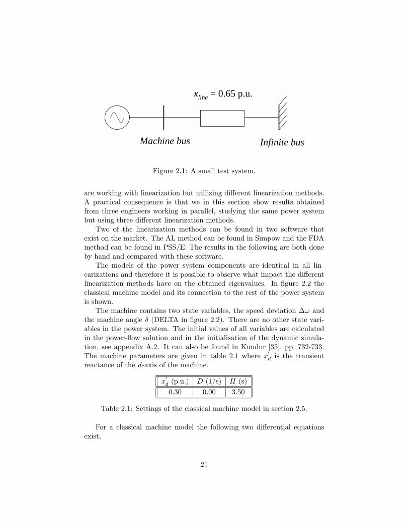
Machine bus Infinite bus

xline = 0.65 p.u.

Figure 2.1: A small test system.

are working with linearization but utilizing different linearization methods.A practical consequence is that we in this section show results obtainedfrom three engineers working in parallel, studying the same power systembut using three different linearization methods.

Two of the linearization methods can be found in two software thatexist on the market. The AL method can be found in Simpow and the FDAmethod can be found in PSS/E. The results in the following are both doneby hand and compared with these software.

The models of the power system components are identical in all lin-earizations and therefore it is possible to observe what impact the differentlinearization methods have on the obtained eigenvalues. In figure 2.2 theclassical machine model and its connection to the rest of the power systemis shown.

The machine contains two state variables, the speed deviation ∆ω andthe machine angle δ (DELTA in figure 2.2). There are no other state vari-ables in the power system. The initial values of all variables are calculatedin the power-flow solution and in the initialisation of the dynamic simula-tion, see appendix A.2. It can also be found in Kundur [35], pp. 732-733.The machine parameters are given in table 2.1 where x

′d is the transient

reactance of the d -axis of the machine.

x′d (p.u.) D (1/s) H (s)0.30 0.00 3.50

Table 2.1: Settings of the classical machine model in section 2.5.

For a classical machine model the following two differential equationsexist,

21

-

+

1D+s2H

DELTA

*

*

-1.

+- W0

s-

+

EFD0

-1Xd'

-1Xd'

ID + jIQ

Tmud

uq

e-j(pi/2-DELTA)

ej(pi/2-DELTA)ure + juim

iqTe

id

PSIQ

PSID

w

Classical machine model

xline

Infinite busMachine bus

id + jiq ire + jiim

ud + juq

Figure 2.2: The classical machine model in a small test system.

∆ω =1

2H(Tm − Te −D ·∆ω) (2.34)

δ = ω0 ·∆ω. (2.35)

The speed deviation ∆ω is equal to ∆ω = ω−ω0ω0

where ω is the rotorspeed of the synchronous machine in radians per second and ω0 is nominalrotor electrical speed in radians per second (ω0 = 2π · f0).

The following two state variables are included in the state vector x as,

x =[

∆ωδ

]. (2.36)

The nine algebraic equations for the machine and the rest of the powersystem are,

0 = −Te + udid + uqiq (2.37)

0 = −ud + ure sin δ − uim cos δ (2.38)

0 = −uq + ure cos δ + uim sin δ (2.39)

22

0 = −id −uq − Efd0

x′d

(2.40)

0 = −iq +ud

x′d

(2.41)

0 = −ure + ureinfinitebus − xlineiim (2.42)

0 = −uim + uiminfinitebus + xlineire (2.43)

0 = −ire + id sin δ + iq cos δ (2.44)

0 = −iim + iq sin δ − id cos δ (2.45)

where id and iq are the stator current of the machine in d - and q-axisrespectively, ud and uq are the stator voltage of the machine in d - and q-axisrespectively, ure and uim are the real and imaginary parts of the positive-sequence voltage of the machine bus, Efd0 is a constant electric field voltage,ire and iim are the real and imaginary parts of the current through the linereactance xline. ureinfinitebus and uiminfinitebus are the real and imaginaryparts of the positive-sequence voltage of the infinite bus.

Efd0 is an internal voltage and can in the literature often be found asE

′as in Kundur [35] or as E

′q as in Andersson [2].

It would have been possible to decrease the number of algebraic equationsand variables above but here we have chosen to follow Johansson [28].

All left-hand sides of equations (2.37) – (2.45) are equal to zero since wewant to have the left-hand side of these equations equal to zero later duringthe linearization using the AL method, see equation (2.10).

We assume that the corresponding nine algebraic variables are includedin the algebraic variable vector v as,

v =

Te

ud

uq

idiqure

uim

ire

iim

. (2.46)

23

In the following sections 2.5.1, 2.5.2, and 2.5.3 the classical machinemodel in figure 2.2 is linearized with the three methods. The results con-cerning the AL method is obtained by hand and from Simpow, the resultsconcerning the FDA method is obtained by hand and from PSS/E, and theresults concerning the CDA method is obtained only by hand.

In the following subsections it is the A-matrix in equation (2.47) thatshould be derived when using the three methods. It contains linear relationsof the left-hand sides ∆ω and ∆δ and the right-hand sides ∆ω and ∆δ,[

∆ω

∆δ

]=

[A11 A12

A21 A22

] [∆ω∆δ

](2.47)

which we recognize as the earlier defined equation (2.7) which we here givea second time.

∆x = A∆x. (2.48)

2.5.1 Linearization of a classical machine using the AL me-thod

Here we apply the AL method that was described in section 2.4.1. In theAL method we linearize equations (2.34) – (2.35), and (2.37) – (2.45) withrespect to the algebraic variables and the state variables as shown in section2.4.1. We get,

∆ω = − 12H

∆Te −D

2H·∆ω (2.49)

∆δ = ω0 ·∆ω (2.50)

0 = −∆Te + id0∆ud + iq0∆uq + ud0∆id + uq0∆iq (2.51)

0 = −∆ud + (ure0 cos δ0 + uim0 sin δ0)∆δ + sin δ0∆ure − cos δ0∆uim (2.52)

0 = −∆uq + (uim0 cos δ0 − ure0 sin δ0)∆δ + cos δ0∆ure + sin δ0∆uim (2.53)

0 = −∆id −1x′d

∆uq (2.54)

24

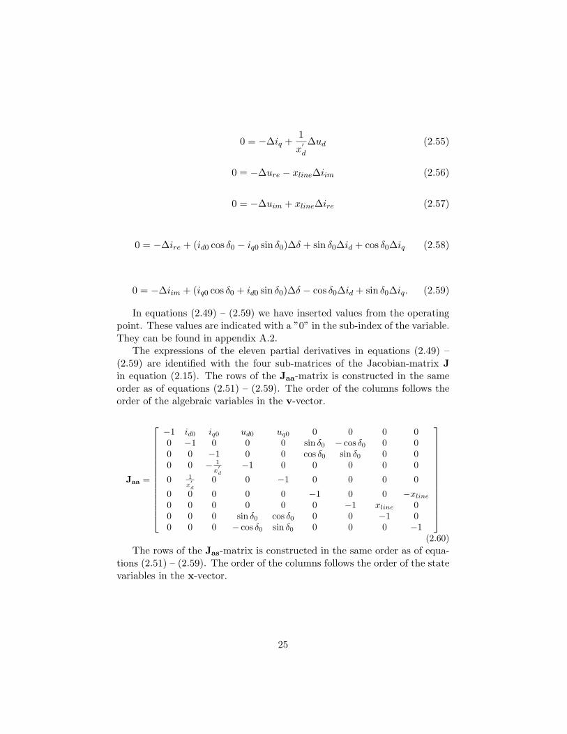
0 = −∆iq +1x′d

∆ud (2.55)

0 = −∆ure − xline∆iim (2.56)

0 = −∆uim + xline∆ire (2.57)

0 = −∆ire + (id0 cos δ0 − iq0 sin δ0)∆δ + sin δ0∆id + cos δ0∆iq (2.58)

0 = −∆iim + (iq0 cos δ0 + id0 sin δ0)∆δ − cos δ0∆id + sin δ0∆iq. (2.59)

In equations (2.49) – (2.59) we have inserted values from the operatingpoint. These values are indicated with a ”0” in the sub-index of the variable.They can be found in appendix A.2.

The expressions of the eleven partial derivatives in equations (2.49) –(2.59) are identified with the four sub-matrices of the Jacobian-matrix Jin equation (2.15). The rows of the Jaa-matrix is constructed in the sameorder as of equations (2.51) – (2.59). The order of the columns follows theorder of the algebraic variables in the v-vector.

Jaa =

−1 id0 iq0 ud0 uq0 0 0 0 00 −1 0 0 0 sin δ0 − cos δ0 0 00 0 −1 0 0 cos δ0 sin δ0 0 00 0 − 1

x′d

−1 0 0 0 0 0

0 1x

′d

0 0 −1 0 0 0 0

0 0 0 0 0 −1 0 0 −xline

0 0 0 0 0 0 −1 xline 00 0 0 sin δ0 cos δ0 0 0 −1 00 0 0 − cos δ0 sin δ0 0 0 0 −1

(2.60)

The rows of the Jas-matrix is constructed in the same order as of equa-tions (2.51) – (2.59). The order of the columns follows the order of the statevariables in the x-vector.

25

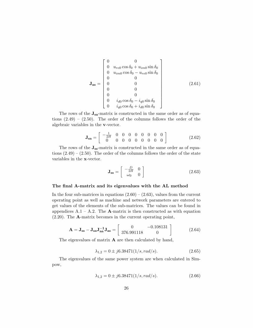
Jas =

0 00 ure0 cos δ0 + uim0 sin δ0

0 uim0 cos δ0 − ure0 sin δ0

0 00 00 00 00 id0 cos δ0 − iq0 sin δ0

0 iq0 cos δ0 + id0 sin δ0

(2.61)

The rows of the Jsa-matrix is constructed in the same order as of equa-tions (2.49) – (2.50). The order of the columns follows the order of thealgebraic variables in the v-vector.

Jsa =[− 1

2H 0 0 0 0 0 0 0 00 0 0 0 0 0 0 0 0

](2.62)

The rows of the Jss-matrix is constructed in the same order as of equa-tions (2.49) – (2.50). The order of the columns follows the order of the statevariables in the x-vector.

Jss =[− D

2H 0ω0 0

](2.63)

The final A-matrix and its eigenvalues with the AL method

In the four sub-matrices in equations (2.60) – (2.63), values from the currentoperating point as well as machine and network parameters are entered toget values of the elements of the sub-matrices. The values can be found inappendices A.1 – A.2. The A-matrix is then constructed as with equation(2.20). The A-matrix becomes in the current operating point,

A = Jss − JsaJ−1aa Jas =

[0 −0.108131

376.991118 0

](2.64)

The eigenvalues of matrix A are then calculated by hand,

λ1,2 = 0± j6.38471(1/s, rad/s). (2.65)

The eigenvalues of the same power system are when calculated in Sim-pow,

λ1,2 = 0± j6.38471(1/s, rad/s). (2.66)

26

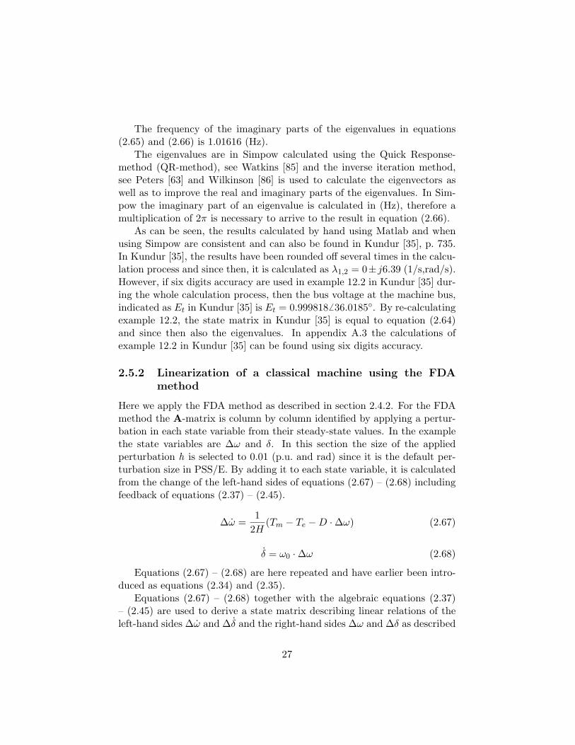
The frequency of the imaginary parts of the eigenvalues in equations(2.65) and (2.66) is 1.01616 (Hz).

The eigenvalues are in Simpow calculated using the Quick Response-method (QR-method), see Watkins [85] and the inverse iteration method,see Peters [63] and Wilkinson [86] is used to calculate the eigenvectors aswell as to improve the real and imaginary parts of the eigenvalues. In Sim-pow the imaginary part of an eigenvalue is calculated in (Hz), therefore amultiplication of 2π is necessary to arrive to the result in equation (2.66).

As can be seen, the results calculated by hand using Matlab and whenusing Simpow are consistent and can also be found in Kundur [35], p. 735.In Kundur [35], the results have been rounded off several times in the calcu-lation process and since then, it is calculated as λ1,2 = 0± j6.39 (1/s,rad/s).However, if six digits accuracy are used in example 12.2 in Kundur [35] dur-ing the whole calculation process, then the bus voltage at the machine bus,indicated as Et in Kundur [35] is Et = 0.9998186 36.0185. By re-calculatingexample 12.2, the state matrix in Kundur [35] is equal to equation (2.64)and since then also the eigenvalues. In appendix A.3 the calculations ofexample 12.2 in Kundur [35] can be found using six digits accuracy.

2.5.2 Linearization of a classical machine using the FDAmethod

Here we apply the FDA method as described in section 2.4.2. For the FDAmethod the A-matrix is column by column identified by applying a pertur-bation in each state variable from their steady-state values. In the examplethe state variables are ∆ω and δ. In this section the size of the appliedperturbation h is selected to 0.01 (p.u. and rad) since it is the default per-turbation size in PSS/E. By adding it to each state variable, it is calculatedfrom the change of the left-hand sides of equations (2.67) – (2.68) includingfeedback of equations (2.37) – (2.45).

∆ω =1

2H(Tm − Te −D ·∆ω) (2.67)

δ = ω0 ·∆ω (2.68)

Equations (2.67) – (2.68) are here repeated and have earlier been intro-duced as equations (2.34) and (2.35).

Equations (2.67) – (2.68) together with the algebraic equations (2.37)– (2.45) are used to derive a state matrix describing linear relations of theleft-hand sides ∆ω and ∆δ and the right-hand sides ∆ω and ∆δ as described

27

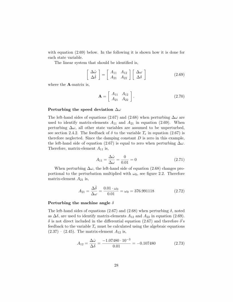
with equation (2.69) below. In the following it is shown how it is done foreach state variable.

The linear system that should be identified is,[∆ω

∆δ

]=

[A11 A12

A21 A22

] [∆ω∆δ

](2.69)

where the A-matrix is,

A =[

A11 A12

A21 A22

]. (2.70)

Perturbing the speed deviation ∆ω

The left-hand sides of equations (2.67) and (2.68) when perturbing ∆ω areused to identify matrix-elements A11 and A21 in equation (2.69). Whenperturbing ∆ω, all other state variables are assumed to be unperturbed,see section 2.4.2. The feedback of δ to the variable Te in equation (2.67) istherefore neglected. Since the damping constant D is zero in this example,the left-hand side of equation (2.67) is equal to zero when perturbing ∆ω.Therefore, matrix-element A11 is,

A11 =∆ω

∆ω=

00.01

= 0 (2.71)

When perturbing ∆ω, the left-hand side of equation (2.68) changes pro-portional to the perturbation multiplied with ω0, see figure 2.2. Thereforematrix-element A21 is,

A21 =∆δ

∆ω=

0.01 · ω0

0.01= ω0 = 376.991118 (2.72)

Perturbing the machine angle δ

The left-hand sides of equations (2.67) and (2.68) when perturbing δ, notedas ∆δ, are used to identify matrix-elements A12 and A22 in equation (2.69).δ is not direct included in the differential equation (2.67) and therefore δ’sfeedback to the variable Te must be calculated using the algebraic equations(2.37) – (2.45). The matrix-element A12 is,

A12 =∆ω

∆δ=−1.07480 · 10−3

0.01= −0.107480 (2.73)

28

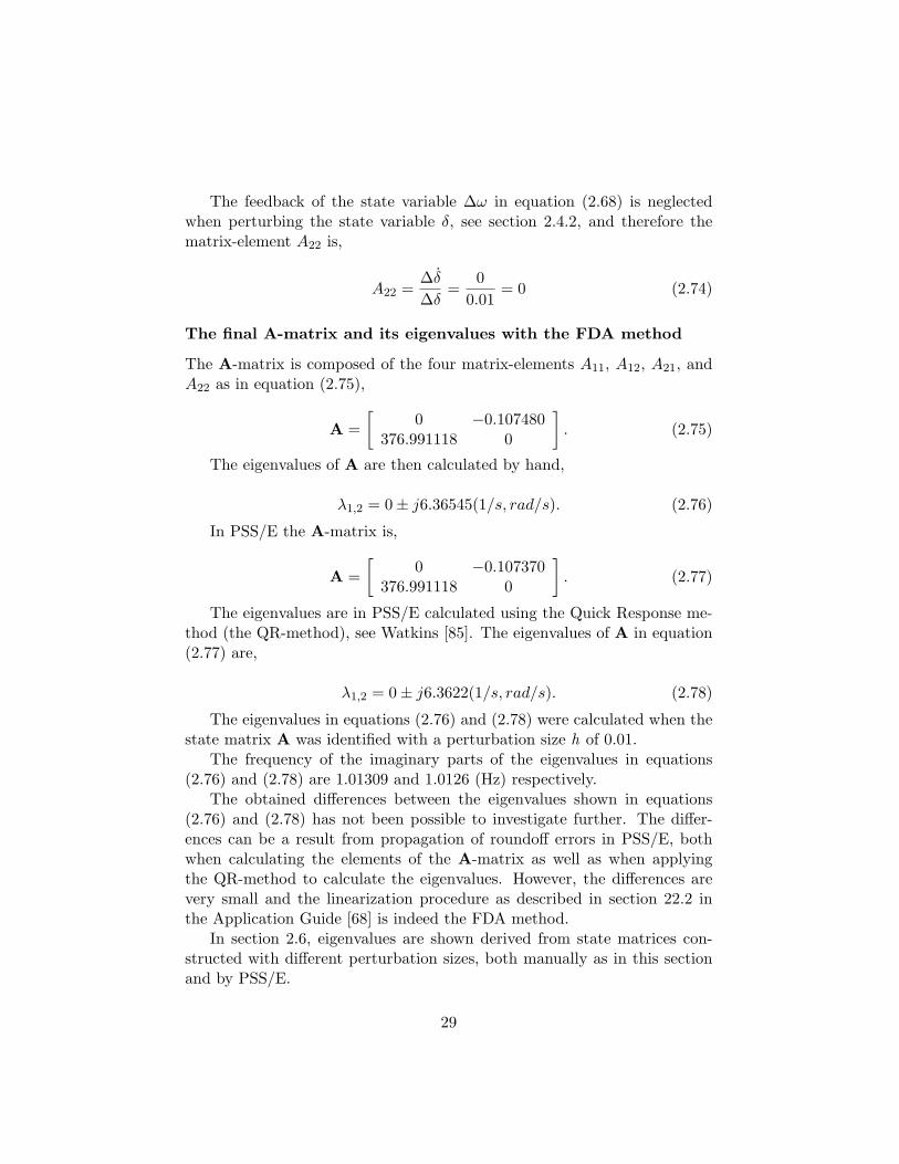
The feedback of the state variable ∆ω in equation (2.68) is neglectedwhen perturbing the state variable δ, see section 2.4.2, and therefore thematrix-element A22 is,

A22 =∆δ

∆δ=

00.01

= 0 (2.74)

The final A-matrix and its eigenvalues with the FDA method

The A-matrix is composed of the four matrix-elements A11, A12, A21, andA22 as in equation (2.75),

A =[

0 −0.107480376.991118 0

]. (2.75)

The eigenvalues of A are then calculated by hand,

λ1,2 = 0± j6.36545(1/s, rad/s). (2.76)

In PSS/E the A-matrix is,

A =[

0 −0.107370376.991118 0

]. (2.77)

The eigenvalues are in PSS/E calculated using the Quick Response me-thod (the QR-method), see Watkins [85]. The eigenvalues of A in equation(2.77) are,

λ1,2 = 0± j6.3622(1/s, rad/s). (2.78)

The eigenvalues in equations (2.76) and (2.78) were calculated when thestate matrix A was identified with a perturbation size h of 0.01.

The frequency of the imaginary parts of the eigenvalues in equations(2.76) and (2.78) are 1.01309 and 1.0126 (Hz) respectively.

The obtained differences between the eigenvalues shown in equations(2.76) and (2.78) has not been possible to investigate further. The differ-ences can be a result from propagation of roundoff errors in PSS/E, bothwhen calculating the elements of the A-matrix as well as when applyingthe QR-method to calculate the eigenvalues. However, the differences arevery small and the linearization procedure as described in section 22.2 inthe Application Guide [68] is indeed the FDA method.

In section 2.6, eigenvalues are shown derived from state matrices con-structed with different perturbation sizes, both manually as in this sectionand by PSS/E.

29

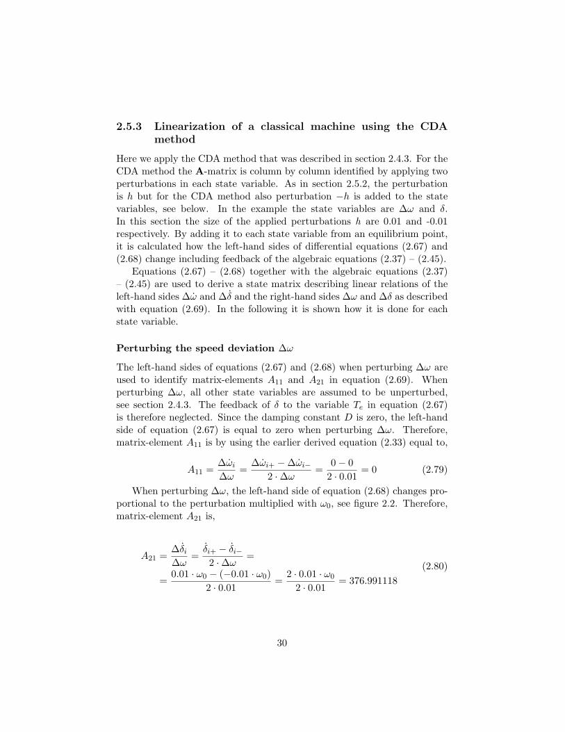
2.5.3 Linearization of a classical machine using the CDAmethod

Here we apply the CDA method that was described in section 2.4.3. For theCDA method the A-matrix is column by column identified by applying twoperturbations in each state variable. As in section 2.5.2, the perturbationis h but for the CDA method also perturbation −h is added to the statevariables, see below. In the example the state variables are ∆ω and δ.In this section the size of the applied perturbations h are 0.01 and -0.01respectively. By adding it to each state variable from an equilibrium point,it is calculated how the left-hand sides of differential equations (2.67) and(2.68) change including feedback of the algebraic equations (2.37) – (2.45).

Equations (2.67) – (2.68) together with the algebraic equations (2.37)– (2.45) are used to derive a state matrix describing linear relations of theleft-hand sides ∆ω and ∆δ and the right-hand sides ∆ω and ∆δ as describedwith equation (2.69). In the following it is shown how it is done for eachstate variable.

Perturbing the speed deviation ∆ω

The left-hand sides of equations (2.67) and (2.68) when perturbing ∆ω areused to identify matrix-elements A11 and A21 in equation (2.69). Whenperturbing ∆ω, all other state variables are assumed to be unperturbed,see section 2.4.3. The feedback of δ to the variable Te in equation (2.67)is therefore neglected. Since the damping constant D is zero, the left-handside of equation (2.67) is equal to zero when perturbing ∆ω. Therefore,matrix-element A11 is by using the earlier derived equation (2.33) equal to,

A11 =∆ωi

∆ω=

∆ωi+ −∆ωi−2 ·∆ω

=0− 0

2 · 0.01= 0 (2.79)

When perturbing ∆ω, the left-hand side of equation (2.68) changes pro-portional to the perturbation multiplied with ω0, see figure 2.2. Therefore,matrix-element A21 is,

A21 =∆δi

∆ω=

δi+ − δi−2 ·∆ω

=

=0.01 · ω0 − (−0.01 · ω0)

2 · 0.01=

2 · 0.01 · ω0

2 · 0.01= 376.991118

(2.80)

30

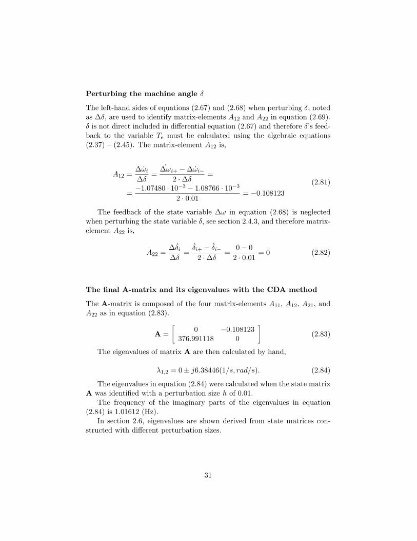
Perturbing the machine angle δ

The left-hand sides of equations (2.67) and (2.68) when perturbing δ, notedas ∆δ, are used to identify matrix-elements A12 and A22 in equation (2.69).δ is not direct included in differential equation (2.67) and therefore δ’s feed-back to the variable Te must be calculated using the algebraic equations(2.37) – (2.45). The matrix-element A12 is,

A12 =∆ωi

∆δ=

∆ωi+ −∆ωi−2 ·∆δ

=

=−1.07480 · 10−3 − 1.08766 · 10−3

2 · 0.01= −0.108123

(2.81)

The feedback of the state variable ∆ω in equation (2.68) is neglectedwhen perturbing the state variable δ, see section 2.4.3, and therefore matrix-element A22 is,

A22 =∆δi

∆δ=

δi+ − δi−2 ·∆δ

=0− 0

2 · 0.01= 0 (2.82)

The final A-matrix and its eigenvalues with the CDA method

The A-matrix is composed of the four matrix-elements A11, A12, A21, andA22 as in equation (2.83).

A =[

0 −0.108123376.991118 0

](2.83)

The eigenvalues of matrix A are then calculated by hand,

λ1,2 = 0± j6.38446(1/s, rad/s). (2.84)

The eigenvalues in equation (2.84) were calculated when the state matrixA was identified with a perturbation size h of 0.01.

The frequency of the imaginary parts of the eigenvalues in equation(2.84) is 1.01612 (Hz).

In section 2.6, eigenvalues are shown derived from state matrices con-structed with different perturbation sizes.

31

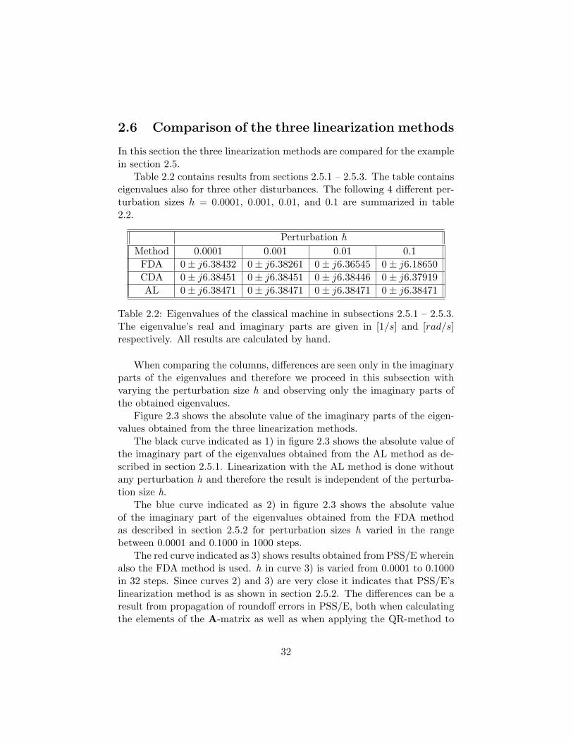
2.6 Comparison of the three linearization methods

In this section the three linearization methods are compared for the examplein section 2.5.

Table 2.2 contains results from sections 2.5.1 – 2.5.3. The table containseigenvalues also for three other disturbances. The following 4 different per-turbation sizes h = 0.0001, 0.001, 0.01, and 0.1 are summarized in table2.2.

Perturbation hMethod 0.0001 0.001 0.01 0.1FDA 0± j6.38432 0± j6.38261 0± j6.36545 0± j6.18650CDA 0± j6.38451 0± j6.38451 0± j6.38446 0± j6.37919AL 0± j6.38471 0± j6.38471 0± j6.38471 0± j6.38471

Table 2.2: Eigenvalues of the classical machine in subsections 2.5.1 – 2.5.3.The eigenvalue’s real and imaginary parts are given in [1/s] and [rad/s]respectively. All results are calculated by hand.

When comparing the columns, differences are seen only in the imaginaryparts of the eigenvalues and therefore we proceed in this subsection withvarying the perturbation size h and observing only the imaginary parts ofthe obtained eigenvalues.

Figure 2.3 shows the absolute value of the imaginary parts of the eigen-values obtained from the three linearization methods.

The black curve indicated as 1) in figure 2.3 shows the absolute value ofthe imaginary part of the eigenvalues obtained from the AL method as de-scribed in section 2.5.1. Linearization with the AL method is done withoutany perturbation h and therefore the result is independent of the perturba-tion size h.

The blue curve indicated as 2) in figure 2.3 shows the absolute valueof the imaginary part of the eigenvalues obtained from the FDA methodas described in section 2.5.2 for perturbation sizes h varied in the rangebetween 0.0001 and 0.1000 in 1000 steps.

The red curve indicated as 3) shows results obtained from PSS/E whereinalso the FDA method is used. h in curve 3) is varied from 0.0001 to 0.1000in 32 steps. Since curves 2) and 3) are very close it indicates that PSS/E’slinearization method is as shown in section 2.5.2. The differences can be aresult from propagation of roundoff errors in PSS/E, both when calculatingthe elements of the A-matrix as well as when applying the QR-method to

32

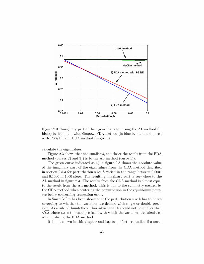
0.0001 0.02 0.04 0.06 0.08 0.16.15

6.2

6.25

6.3

6.35

6.4

6.45

Perturbation, h

w (r

ad/s

ec)

1) AL method

2) FDA method

3) FDA method with PSS/E

4) CDA method

Figure 2.3: Imaginary part of the eigenvalue when using the AL method (inblack) by hand and with Simpow, FDA method (in blue by hand and in redwith PSS/E), and CDA method (in green).

calculate the eigenvalues.Figure 2.3 shows that the smaller h, the closer the result from the FDA

method (curves 2) and 3)) is to the AL method (curve 1)).The green curve indicated as 4) in figure 2.3 shows the absolute value

of the imaginary part of the eigenvalues from the CDA method describedin section 2.5.3 for perturbation sizes h varied in the range between 0.0001and 0.1000 in 1000 steps. The resulting imaginary part is very close to theAL method in figure 2.3. The results from the CDA method is almost equalto the result from the AL method. This is due to the symmetry created bythe CDA method when centering the perturbation in the equilibrium point,see below concerning truncation error.

In Smed [79] it has been shown that the perturbation size h has to be setaccording to whether the variables are defined with single or double preci-sion. As a rule of thumb the author advice that h should not be smaller than√

tol where tol is the used precision with which the variables are calculatedwhen utilizing the FDA method.

It is not shown in this chapter and has to be further studied if a small

33

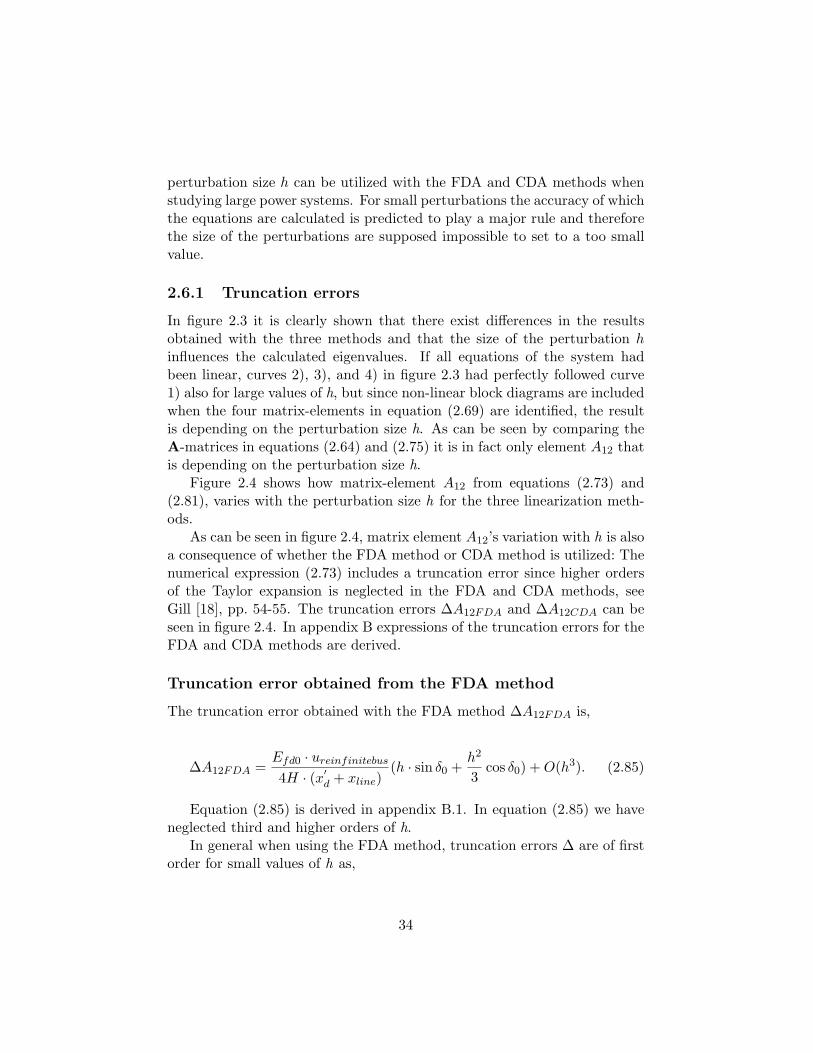
perturbation size h can be utilized with the FDA and CDA methods whenstudying large power systems. For small perturbations the accuracy of whichthe equations are calculated is predicted to play a major rule and thereforethe size of the perturbations are supposed impossible to set to a too smallvalue.

2.6.1 Truncation errors

In figure 2.3 it is clearly shown that there exist differences in the resultsobtained with the three methods and that the size of the perturbation hinfluences the calculated eigenvalues. If all equations of the system hadbeen linear, curves 2), 3), and 4) in figure 2.3 had perfectly followed curve1) also for large values of h, but since non-linear block diagrams are includedwhen the four matrix-elements in equation (2.69) are identified, the resultis depending on the perturbation size h. As can be seen by comparing theA-matrices in equations (2.64) and (2.75) it is in fact only element A12 thatis depending on the perturbation size h.

Figure 2.4 shows how matrix-element A12 from equations (2.73) and(2.81), varies with the perturbation size h for the three linearization meth-ods.

As can be seen in figure 2.4, matrix element A12’s variation with h is alsoa consequence of whether the FDA method or CDA method is utilized: Thenumerical expression (2.73) includes a truncation error since higher ordersof the Taylor expansion is neglected in the FDA and CDA methods, seeGill [18], pp. 54-55. The truncation errors ∆A12FDA and ∆A12CDA can beseen in figure 2.4. In appendix B expressions of the truncation errors for theFDA and CDA methods are derived.

Truncation error obtained from the FDA method

The truncation error obtained with the FDA method ∆A12FDA is,

∆A12FDA =Efd0 · ureinfinitebus

4H · (x′d + xline)

(h · sin δ0 +h2

3cos δ0) + O(h3). (2.85)

Equation (2.85) is derived in appendix B.1. In equation (2.85) we haveneglected third and higher orders of h.

In general when using the FDA method, truncation errors ∆ are of firstorder for small values of h as,

34

0.0001 0.02 0.04 0.06 0.08 0.1-0.109

-0.107

-0.105

-0.103

-0.101

Perturbation, h

A12 A12 FDA

A12 CDA

A12 FDA∆

A12 CDA∆

A12 AL

A12 FDA-mod∆

Figure 2.4: Matrix element A12 derived when using the FDA method (inblue) and the CDA method (in green). The truncation error when using theFDA method ∆A12FDA is marked as the distance between the black and theblue curve. The truncation error when using the CDA method ∆A12CDA

is marked as the distance between the black and the green curve. The redcurve shows A12 when having a linear relation with h.

∆ = O(h). (2.86)

In figure 2.4 we can see that the truncation error ∆A12FDA indeed hasalmost a linear relation with h as shown in equation (2.85). If the truncationerror would consist only of the first term in equation (2.85), as,

∆A12FDA−mod =Efd0 · ureinfinitebus

4H · (x′d + xline)

h · sin δ0 (2.87)

we would obtain the red curve in figure 2.4 describing how A12 would developwith h. In figure 2.4 it is possible to see that the distance between the blue

35

and the red curve is equal to ∆A12CDA. This can also be observed bycomparing equations (2.85), (2.87), and equation (2.88) below.

The matrix-elements other than A12 are independent of the size of hsince the equations are linear.

Truncation error obtained from the CDA method

The truncation error obtained with the CDA method ∆A12CDA is,

∆A12CDA =Efd0 · ureinfinitebus

4H · (x′d + xline)

cos δ0 · (h2

3− h4

60) + O(h6). (2.88)

Equation (2.88) is derived in appendix B.2. In equation (2.88) we haveneglected sixth and higher orders of h.

In general when using the CDA method, truncation errors ∆ are ofsecond order for small values of h as,

∆ = O(h2). (2.89)

In figure 2.4 we can see that the truncation error ∆A12CDA indeed isvery small as shown in equation (2.88).

In Taylor [81, 82] a method is shown to decrease the truncation errorwhen using the CDA method. The method sets the size of the perturbationto minimize the truncation error as much as possible.

2.7 Large-disturbance stability analysis

In small-signal stability analysis, conclusions are drawn from small distur-bances ∆. In this section we will apply large disturbances for the samepower system and see if we obtain similar results as in sections 2.5 and 2.6.

Curves 2), 3), and 4) in figure 2.3 showed the result when perturbationswere large. The FDA and CDA methods include non-linear feedback fromthe algebraic equations and we have seen in figure 2.3 that the imaginarypart of the eigenvalue-pair is as low as 6.2 (rad/s) for large perturbations hwhen using the FDA method.

The results from the linearization has in this section been comparedwith time-domain simulations of the power system where a solid three-phasefault has been applied on the machine bus in figure 2.2 with different faultdurations tc. In figure 2.5 the rotor angle δ and speed deviation ∆ω for

36

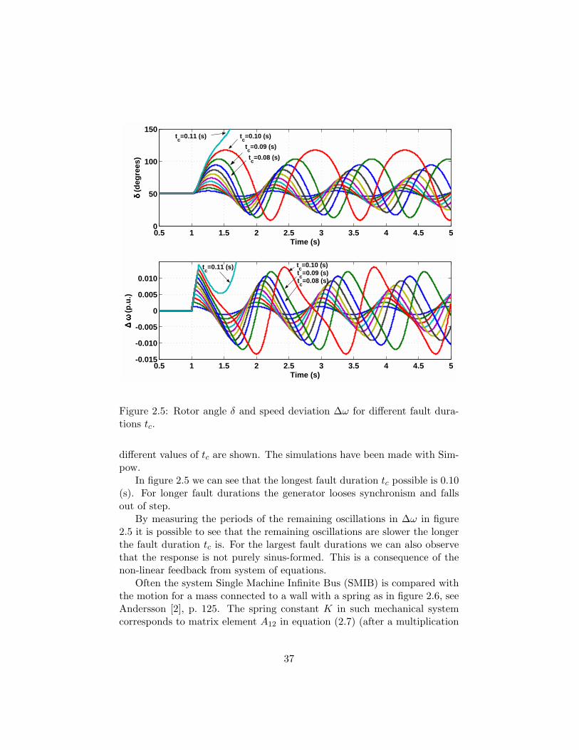
0.5 1 1.5 2 2.5 3 3.5 4 4.5 50

50

100

150

Time (s)

δδ δδ (d

egre

es)

0.5 1 1.5 2 2.5 3 3.5 4 4.5 5-0.015

-0.010

-0.005

0

0.005

0.010

Time (s)

∆∆ ∆∆ ωω ωω

(p.u

.)tc=0.11 (s)

tc=0.11 (s)

tc=0.10 (s) tc=0.09 (s)

tc=0.08 (s)

tc=0.10 (s) tc=0.09 (s) tc=0.08 (s)

Figure 2.5: Rotor angle δ and speed deviation ∆ω for different fault dura-tions tc.

different values of tc are shown. The simulations have been made with Sim-pow.

In figure 2.5 we can see that the longest fault duration tc possible is 0.10(s). For longer fault durations the generator looses synchronism and fallsout of step.

By measuring the periods of the remaining oscillations in ∆ω in figure2.5 it is possible to see that the remaining oscillations are slower the longerthe fault duration tc is. For the largest fault durations we can also observethat the response is not purely sinus-formed. This is a consequence of thenon-linear feedback from system of equations.

Often the system Single Machine Infinite Bus (SMIB) is compared withthe motion for a mass connected to a wall with a spring as in figure 2.6, seeAndersson [2], p. 125. The spring constant K in such mechanical systemcorresponds to matrix element A12 in equation (2.7) (after a multiplication

37

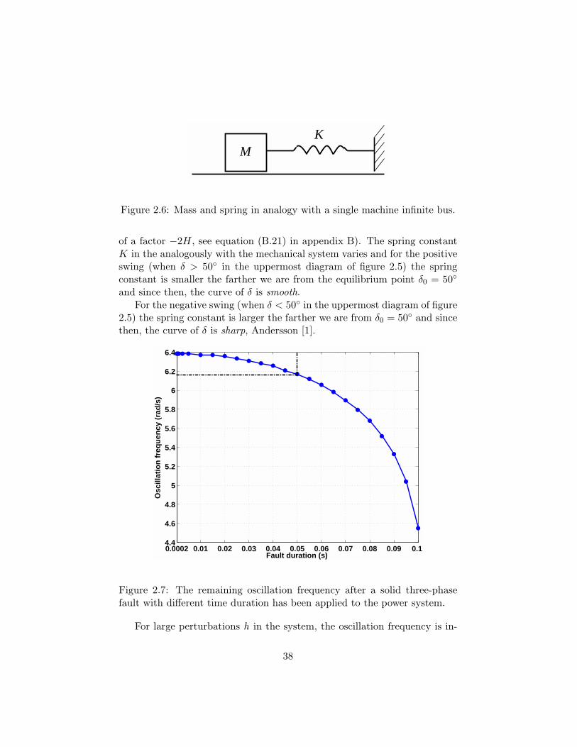
MK

Figure 2.6: Mass and spring in analogy with a single machine infinite bus.

of a factor −2H, see equation (B.21) in appendix B). The spring constantK in the analogously with the mechanical system varies and for the positiveswing (when δ > 50 in the uppermost diagram of figure 2.5) the springconstant is smaller the farther we are from the equilibrium point δ0 = 50

and since then, the curve of δ is smooth.For the negative swing (when δ < 50 in the uppermost diagram of figure

2.5) the spring constant is larger the farther we are from δ0 = 50 and sincethen, the curve of δ is sharp, Andersson [1].

0.0002 0.01 0.02 0.03 0.04 0.05 0.06 0.07 0.08 0.09 0.1 4.4

4.6

4.8

5

5.2

5.4

5.6

5.8

6

6.2

6.4

Fault duration (s)

Osc

illat

ion

freq

uenc

y (r

ad/s

)

Figure 2.7: The remaining oscillation frequency after a solid three-phasefault with different time duration has been applied to the power system.

For large perturbations h in the system, the oscillation frequency is in-

38

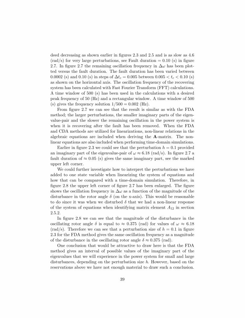
deed decreasing as shown earlier in figures 2.3 and 2.5 and is as slow as 4.6(rad/s) for very large perturbations, see Fault duration = 0.10 (s) in figure2.7. In figure 2.7 the remaining oscillation frequency in ∆ω has been plot-ted versus the fault duration. The fault duration has been varied between0.0002 (s) and 0.10 (s) in steps of ∆tc = 0.005 between 0.005 < tc < 0.10 (s)as shown on the horizontal axis. The oscillation frequency of the recoveringsystem has been calculated with Fast Fourier Transform (FFT) calculations.A time window of 500 (s) has been used in the calculations with a desiredpeak frequency of 50 (Hz) and a rectangular window. A time window of 500(s) gives the frequency solution 1/500 = 0.002 (Hz).

From figure 2.7 we can see that the result is similar as with the FDAmethod; the larger perturbations, the smaller imaginary parts of the eigen-value-pair and the slower the remaining oscillation in the power system iswhen it is recovering after the fault has been removed. When the FDAand CDA methods are utilized for linearizations, non-linear relations in thealgebraic equations are included when deriving the A-matrix. The non-linear equations are also included when performing time-domain simulations.

Earlier in figure 2.3 we could see that the perturbation h = 0.1 providedan imaginary part of the eigenvalue-pair of ω ≈ 6.18 (rad/s). In figure 2.7 afault duration of ≈ 0.05 (s) gives the same imaginary part, see the markedupper left corner.

We could further investigate how to interpret the perturbations we haveadded to one state variable when linearizing the system of equations andhow that can be compared with a time-domain simulation. Therefore, infigure 2.8 the upper left corner of figure 2.7 has been enlarged. The figureshows the oscillation frequency in ∆ω as a function of the magnitude of thedisturbance in the rotor angle δ (on the x-axis). This would be reasonableto do since it was when we disturbed δ that we had a non-linear responseof the system of equations when identifying matrix element A12 in section2.5.2.

In figure 2.8 we can see that the magnitude of the disturbance in theoscillating rotor angle δ is equal to ≈ 0.375 (rad) for values of ω ≈ 6.18(rad/s). Therefore we can see that a perturbation size of h = 0.1 in figure2.3 for the FDA method gives the same oscillation frequency as a magnitudeof the disturbance in the oscillating rotor angle δ ≈ 0.375 (rad).

One conclusion that would be attractive to draw here is that the FDAmethod gives an interval of possible values of the imaginary part of theeigenvalues that we will experience in the power system for small and largedisturbances, depending on the perturbation size h. However, based on thereservations above we have not enough material to draw such a conclusion.

39

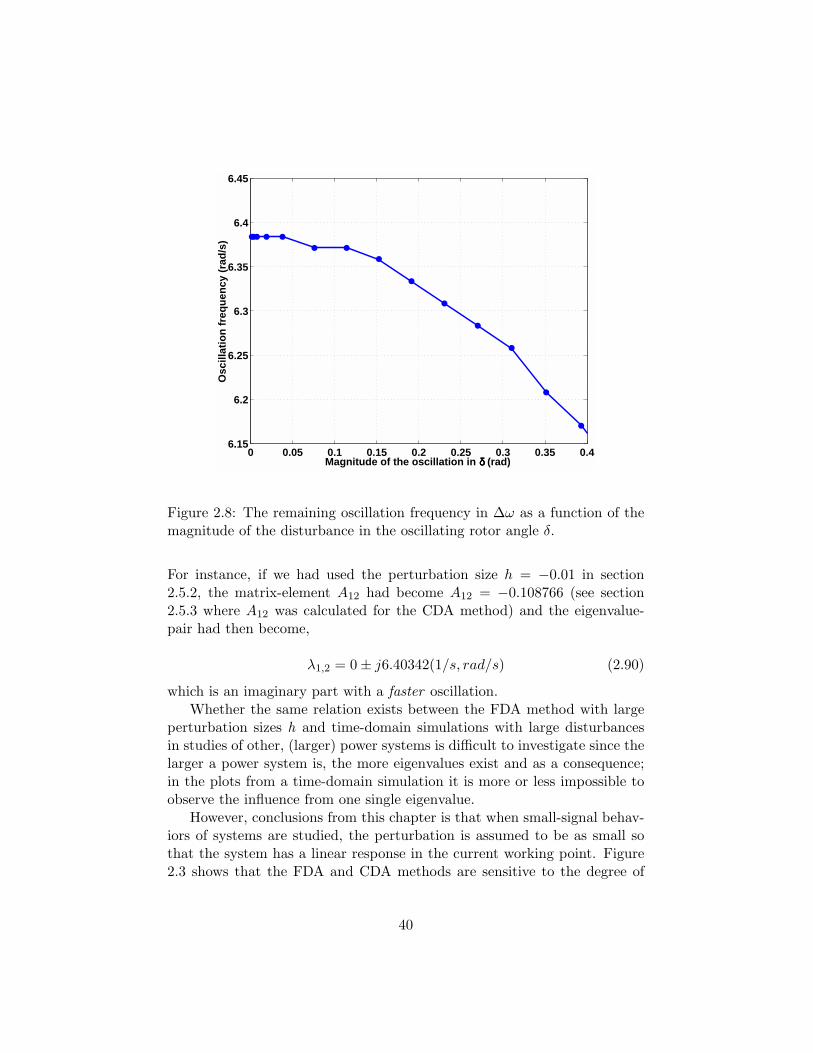
0 0.05 0.1 0.15 0.2 0.25 0.3 0.35 0.46.15

6.2

6.25

6.3

6.35

6.4

6.45

Osc

illat

ion

freq

uenc

y (r

ad/s

)

Magnitude of the oscillation in δδδδ (rad)

Figure 2.8: The remaining oscillation frequency in ∆ω as a function of themagnitude of the disturbance in the oscillating rotor angle δ.

For instance, if we had used the perturbation size h = −0.01 in section2.5.2, the matrix-element A12 had become A12 = −0.108766 (see section2.5.3 where A12 was calculated for the CDA method) and the eigenvalue-pair had then become,

λ1,2 = 0± j6.40342(1/s, rad/s) (2.90)

which is an imaginary part with a faster oscillation.Whether the same relation exists between the FDA method with large

perturbation sizes h and time-domain simulations with large disturbancesin studies of other, (larger) power systems is difficult to investigate since thelarger a power system is, the more eigenvalues exist and as a consequence;in the plots from a time-domain simulation it is more or less impossible toobserve the influence from one single eigenvalue.

However, conclusions from this chapter is that when small-signal behav-iors of systems are studied, the perturbation is assumed to be as small sothat the system has a linear response in the current working point. Figure2.3 shows that the FDA and CDA methods are sensitive to the degree of

40

non-linearity of the equations of the studied system as well as to the size ofthe perturbation h. The sensitivity is largest for the FDA method.

2.8 Summary

Three linearization methods have been evaluated in this chapter. The ana-lytical linearization is achieved by writing the models in terms of the mostelementary components for which a linearization formula is known. Theforward-difference and center-difference approximation methods are numer-ical methods.

The chapter analyzes results obtained from three engineers working inparallel, studying the same power system but using three different lineariza-tion methods. The aim in the chapter has been to show that the usedlinearization method in a power system simulation software has an impacton the obtained eigenvalues. Attention should be paid to this when analyz-ing a power system with different software since differences can be generatedfrom the used linearization methods.

It has been shown that the perturbation size h in the forward-differenceapproximation method influences the calculated eigenvalues. However, forsmall values of the perturbation, results from all the methods are very sim-ilar. When analyzing the electromechanical mode of a small power system,the impact of the difference in linearization methods were investigated.

The results from the numerical center-difference approximation methodare very close to the analytical linearization method.

It is not shown in this chapter and has to be further studied if a smallperturbation size h can be utilized when studying large power systems. Forsmall perturbations the accuracy of which the equations are calculated ispredicted to play an important rule.

The larger perturbation size when using the forward-difference approx-imation method, the smaller imaginary parts of the eigenvalue-pair is ob-tained. This is in conformity with time-domain simulations of the powersystem in the chapter; the larger perturbations the power system is goingthrough, the slower the responding oscillation is when the system is recov-ering after the fault has been removed. Whether the same conformity areobtained also in studies of other power systems could be further investigatedfor the forward-difference approximation method.

The forward-difference approximation and center-difference approxima-tion methods are sensitive to the degree of non-linearity of the equationsof the studied system as well as to the size of the perturbation h. The

41

sensitivity is largest for the forward-difference approximation method.

42

Chapter 3

Modelling the power systemin the thesis

Some formulations and fundamentals of the modelling of the power systemin the thesis has to be mentioned. In this chapter we explain some modellingof the power system as well as comment specific models that are simulated.

3.1 Simulations in instantaneous value mode

The electrical state of the three-phase power system is in the thesis modelledin instantaneous value mode. When using this mode, phase currents andphase voltages do not necessary have to be sinusoidal, they can have any ar-bitrary form. The detailed possibility of modelling is of certain importancefor us since we want to model the thyristor switchings in the power gridin detail. Other names that can be found in the literature for character-izing this mode of simulation are momentary values, electromagnetic tran-sients, and alternative transients program simulations (ATP-simulations),see PSCAD [66], and Persson [57].

3.1.1 The dq0 -representation

To speed up used computer time, the used software in the thesis transformsthree-phase voltages and currents, below indicated as abc-quantities, andrepresent them into a coordinate system called the dq0 -system, [75]. Figure3.1 shows phase voltage ua which we here refer to as one of the abc-quantitiesof a three-phase voltage. During normal conditions the abc-quantities aresinus formed with the power frequency, see the phase voltage for 1.033 <

43

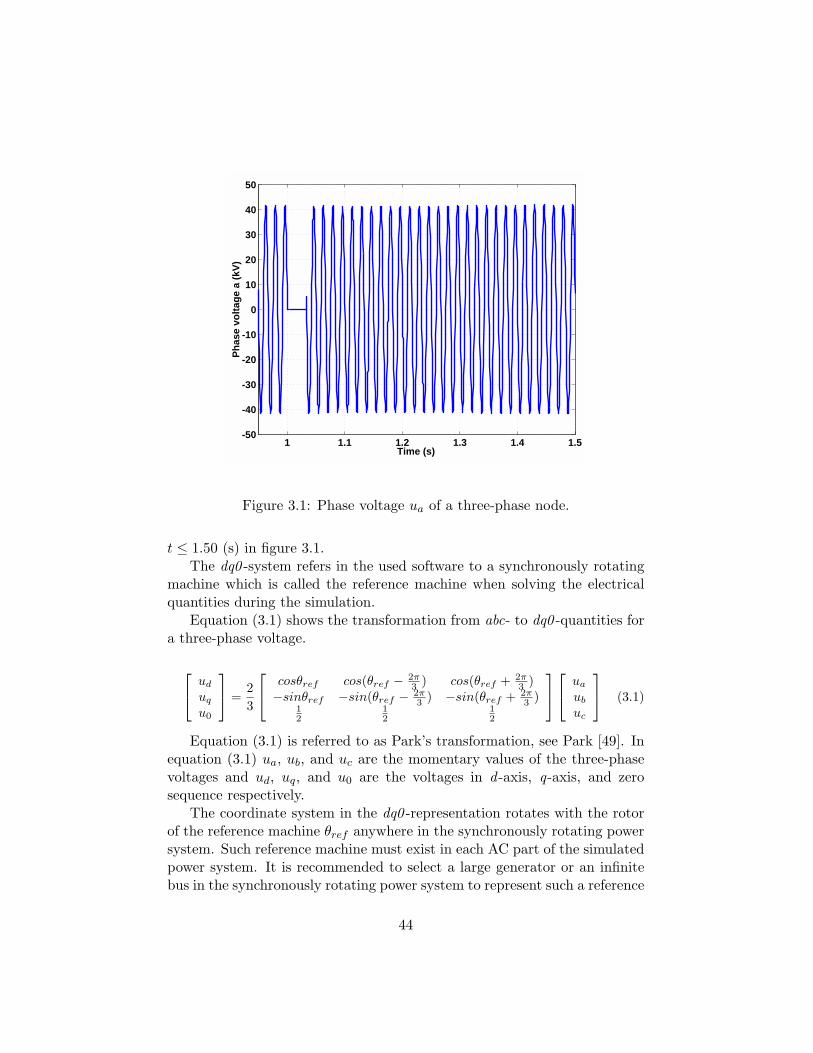
1 1.1 1.2 1.3 1.4 1.5-50

-40

-30

-20

-10

0

10

20

30

40

50

Time (s)

Pha

se v

olta

ge a

(kV

)

Figure 3.1: Phase voltage ua of a three-phase node.

t ≤ 1.50 (s) in figure 3.1.The dq0 -system refers in the used software to a synchronously rotating

machine which is called the reference machine when solving the electricalquantities during the simulation.

Equation (3.1) shows the transformation from abc- to dq0 -quantities fora three-phase voltage.

ud

uq

u0

=23

cosθref cos(θref − 2π3 ) cos(θref + 2π

3 )−sinθref −sin(θref − 2π

3 ) −sin(θref + 2π3 )

12

12

12

ua

ub

uc

(3.1)

Equation (3.1) is referred to as Park’s transformation, see Park [49]. Inequation (3.1) ua, ub, and uc are the momentary values of the three-phasevoltages and ud, uq, and u0 are the voltages in d -axis, q-axis, and zerosequence respectively.

The coordinate system in the dq0 -representation rotates with the rotorof the reference machine θref anywhere in the synchronously rotating powersystem. Such reference machine must exist in each AC part of the simulatedpower system. It is recommended to select a large generator or an infinitebus in the synchronously rotating power system to represent such a reference

44

machine, see Aneros [4], p. 18. The abbreviation AC stands for AlternatingCurrent.

The angle θref is defined as,

θref = 2πf0 · t + θr (3.2)

where f0 is the power frequency (Hz), θr is the load angle of the referencemachine (radians), and t is actual simulated time (s). θref is given in radians.

The load angle θr has the following relation with the per unit speeddeviation ∆ω of the reference machine,

θr = ω0∆ω (3.3)

where ω0 is nominal rotor speed (ω0 = 2πf0) in radians/s. The per unitspeed deviation ∆ω is in (p.u.).

From equation (3.3) we can see that the time-derivative of θr is relatedto the speed deviation ∆ω of the reference machine and therefore also theactual frequency of the power system; If the frequency decreases in thepower system, ∆ω will become negative which gives a negative derivative toθr, according to equation (3.3), so that θr decreases.

From equation (3.2) we can then see that a decreasing θr ”slows down”the development of θref and as a consequence, the dq0 -system rotates slowersince it rotates with θref as shown in equation (3.1). Therefore, the dq0 -system follows the actual frequency of the power system.

In the upper part of figure 3.2 it is shown how ∆ω decreases for thereference machine and becomes negative when the frequency in a powersystem decreases at t = 5 (s) according to a sudden increase in the realpower consumption in the power system. This gives a negative derivative toθr according to equation (3.3) so that θr decreases as well. This is shown inthe lower part of figure 3.2. The power system contains two areas containingone synchronous machine each, feeding a load placed between the two areas.

Since the reference machine in this case is equipped with a secondaryfrequency control, ∆ω returns soon to ≈ 0 which gives almost zero time-derivative to θr according to equation (3.3) and therefore θr remains at theend (t ≈ 50 (s)) almost to a constant value ≈ −8 (radians).

As a consequence of that θr has decreased as shown in figure 3.2, θref inequation (3.2) has ”slowed down” and the dq0 -system is at t = 50 (s) againrotating with power frequency but nowadays θr (radians) behind, comparedto the position it would have had if the power consumption of the powersystem would had remained undisturbed.

45

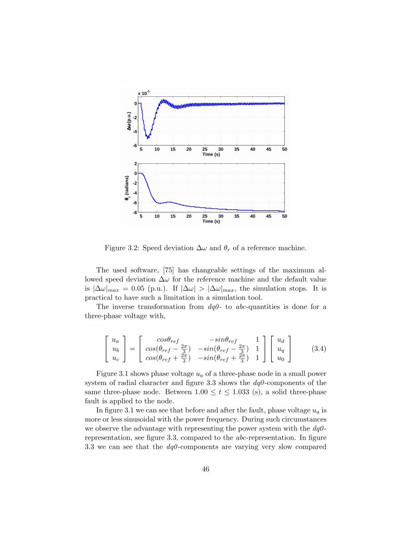
5 10 15 20 25 30 35 40 45 50-6

-4

-2

0

x 10-3

Time (s)

∆∆ ∆∆ ωω ωω (p

.u.)

5 10 15 20 25 30 35 40 45 50-8

-6

-4

-2

0

2

Time (s)

θθ θθ r (rad

ians

)

Figure 3.2: Speed deviation ∆ω and θr of a reference machine.

The used software, [75] has changeable settings of the maximum al-lowed speed deviation ∆ω for the reference machine and the default valueis |∆ω|max = 0.05 (p.u.). If |∆ω| > |∆ω|max, the simulation stops. It ispractical to have such a limitation in a simulation tool.

The inverse transformation from dq0 - to abc-quantities is done for athree-phase voltage with,

ua

ub

uc

=

cosθref −sinθref 1cos(θref − 2π

3 ) −sin(θref − 2π3 ) 1

cos(θref + 2π3 ) −sin(θref + 2π

3 ) 1

ud

uq

u0

(3.4)

Figure 3.1 shows phase voltage ua of a three-phase node in a small powersystem of radial character and figure 3.3 shows the dq0 -components of thesame three-phase node. Between 1.00 ≤ t ≤ 1.033 (s), a solid three-phasefault is applied to the node.

In figure 3.1 we can see that before and after the fault, phase voltage ua ismore or less sinusoidal with the power frequency. During such circumstanceswe observe the advantage with representing the power system with the dq0 -representation, see figure 3.3, compared to the abc-representation. In figure3.3 we can see that the dq0 -components are varying very slow compared

46

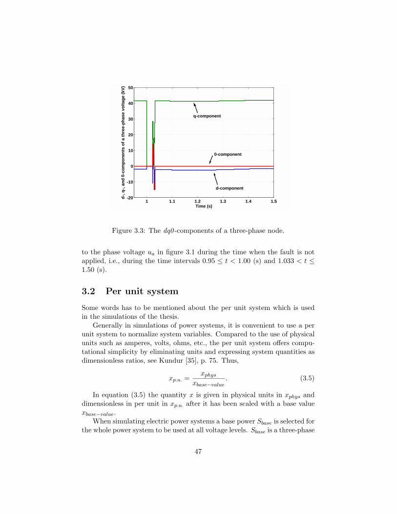
1 1.1 1.2 1.3 1.4 1.5-20

-10

0

10

20

30

40

50

Time (s)

d-, q

-, an

d 0-

com

pone

nts

of a

thre

e-ph

ase

volta

ge (k

V)

q-component

0-component

d-component

Figure 3.3: The dq0 -components of a three-phase node.

to the phase voltage ua in figure 3.1 during the time when the fault is notapplied, i.e., during the time intervals 0.95 ≤ t < 1.00 (s) and 1.033 < t ≤1.50 (s).

3.2 Per unit system

Some words has to be mentioned about the per unit system which is usedin the simulations of the thesis.

Generally in simulations of power systems, it is convenient to use a perunit system to normalize system variables. Compared to the use of physicalunits such as amperes, volts, ohms, etc., the per unit system offers compu-tational simplicity by eliminating units and expressing system quantities asdimensionless ratios, see Kundur [35], p. 75. Thus,

xp.u. =xphys

xbase−value. (3.5)

In equation (3.5) the quantity x is given in physical units in xphys anddimensionless in per unit in xp.u. after it has been scaled with a base valuexbase−value.

When simulating electric power systems a base power Sbase is selected forthe whole power system to be used at all voltage levels. Sbase is a three-phase

47

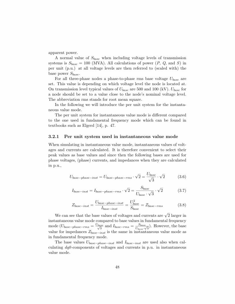
apparent power.A normal value of Sbase when including voltage levels of transmission

systems is Sbase = 100 (MVA). All calculations of power (P, Q, and S ) inper unit (p.u.) at all voltage levels are then referred to (scaled with) thebase power Sbase.

For all three-phase nodes a phase-to-phase rms base voltage Ubase areset. This value is depending on which voltage level the node is located at.On transmission level typical values of Ubase are 500 and 100 (kV). Ubase fora node should be set to a value close to the node’s nominal voltage level.The abbreviation rms stands for root mean square.

In the following we will introduce the per unit system for the instanta-neous value mode.

The per unit system for instantaneous value mode is different comparedto the one used in fundamental frequency mode which can be found intextbooks such as Elgerd [14], p. 47.

3.2.1 Per unit system used in instantaneous value mode

When simulating in instantaneous value mode, instantaneous values of volt-ages and currents are calculated. It is therefore convenient to select theirpeak values as base values and since then the following bases are used forphase voltages, (phase) currents, and impedances when they are calculatedin p.u.,

Ubase−phase−inst = Ubase−phase−rms ·√

2 =Ubase√

3·√

2 (3.6)

Ibase−inst = Ibase−phase−rms ·√

2 =Sbase

Ubase ·√

3·√

2 (3.7)

Zbase−inst =Ubase−phase−inst

Ibase−inst=

U2base

Sbase= Zbase−rms (3.8)

We can see that the base values of voltages and currents are√

2 larger ininstantaneous value mode compared to base values in fundamental frequencymode (Ubase−phase−rms = Ubase√

3and Ibase−rms = Sbase

Ubase·√

3). However, the base

value for impedances Zbase−inst is the same in instantaneous value mode asin fundamental frequency mode.

The base values Ubase−phase−inst and Ibase−inst are used also when cal-culating dq0 -components of voltages and currents in p.u. in instantaneousvalue mode.

48

A + ucap - B

D L

C

irea

icapiline

Figure 3.4: Basic scheme of one phase of the TCSC.

3.3 The original model of the Thyristor-ControlledSeries Capacitor

The basic scheme of the Thyristor-Controlled Series Capacitor (TCSC) isshown in figure 3.4. It consists of a series compensating capacitor C shuntedby a Thyristor-Controlled Reactor (TCR) L.

Assume that the thyristor valve is initially open and that the line currentiline produces a voltage ucap across the fixed series compensating capacitorC as illustrated in figure 3.5 between 5.01 < t < E (s). Suppose that thethyristor-controlled reactor L is to be turned on at point of time E. Asseen, at the instant of turn-on E, the capacitor voltage ucap is negative, theline current iline is positive and thus charging the capacitor in the positivedirection, see Hingorani [20]. Because of the negative voltage ucap over thecapacitor C the current irea becomes negative when the thyristor-controlledreactor is turned on. Here the reverse thyristor is conducting, see the upperthyristor in figure 3.4.

The reverse thyristor stops conducting when the current irea crosses zeroas shown in point of time F in figure 3.5.

When none of the thyristors are conducting, the currents iline (in red)and icap (in blue) are equal, see for instance time interval F ≤ t ≤ G infigure 3.5.

One half period later the procedure described above repeats but now

49

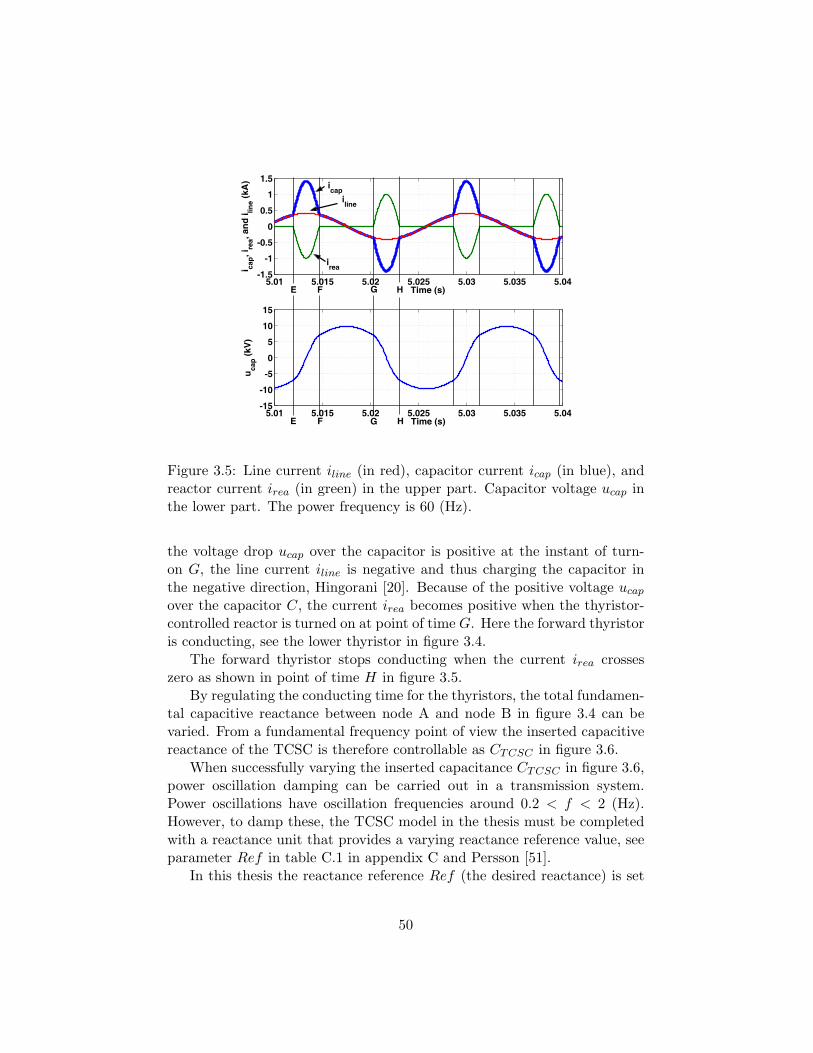
5.01 5.015 5.02 5.025 5.03 5.035 5.04-1.5

-1

-0.5

0

0.5

1

1.5

Time (s)

i cap, i

rea, a

nd i lin

e (kA

)

5.01 5.015 5.02 5.025 5.03 5.035 5.04-15

-10

-5

0

5

10

15

Time (s)

u cap (k

V)

iline icap

irea

E F

E F

G

G

H

H

Figure 3.5: Line current iline (in red), capacitor current icap (in blue), andreactor current irea (in green) in the upper part. Capacitor voltage ucap inthe lower part. The power frequency is 60 (Hz).

the voltage drop ucap over the capacitor is positive at the instant of turn-on G, the line current iline is negative and thus charging the capacitor inthe negative direction, Hingorani [20]. Because of the positive voltage ucap

over the capacitor C, the current irea becomes positive when the thyristor-controlled reactor is turned on at point of time G. Here the forward thyristoris conducting, see the lower thyristor in figure 3.4.

The forward thyristor stops conducting when the current irea crosseszero as shown in point of time H in figure 3.5.

By regulating the conducting time for the thyristors, the total fundamen-tal capacitive reactance between node A and node B in figure 3.4 can bevaried. From a fundamental frequency point of view the inserted capacitivereactance of the TCSC is therefore controllable as CTCSC in figure 3.6.

When successfully varying the inserted capacitance CTCSC in figure 3.6,power oscillation damping can be carried out in a transmission system.Power oscillations have oscillation frequencies around 0.2 < f < 2 (Hz).However, to damp these, the TCSC model in the thesis must be completedwith a reactance unit that provides a varying reactance reference value, seeparameter Ref in table C.1 in appendix C and Persson [51].

In this thesis the reactance reference Ref (the desired reactance) is set

50

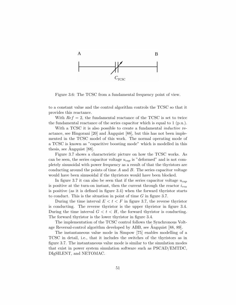
A B

CTCSC

Figure 3.6: The TCSC from a fundamental frequency point of view.

to a constant value and the control algorithm controls the TCSC so that itprovides this reactance.

With Ref = 2, the fundamental reactance of the TCSC is set to twicethe fundamental reactance of the series capacitor which is equal to 1 (p.u.).

With a TCSC it is also possible to create a fundamental inductive re-actance, see Hingorani [20] and Angquist [88], but this has not been imple-mented in the TCSC model of this work. The normal operating mode ofa TCSC is known as ”capacitive boosting mode” which is modelled in thisthesis, see Angquist [88].

Figure 3.7 shows a characteristic picture on how the TCSC works. Ascan be seen, the series capacitor voltage ucap is ”deformed” and is not com-pletely sinusoidal with power frequency as a result of that the thyristors areconducting around the points of time A and B. The series capacitor voltagewould have been sinusoidal if the thyristors would have been blocked.

In figure 3.7 it can also be seen that if the series capacitor voltage ucap

is positive at the turn-on instant, then the current through the reactor irea

is positive (as it is defined in figure 3.4) when the forward thyristor startsto conduct. This is the situation in point of time G in figure 3.7.

During the time interval E < t < F in figure 3.7, the reverse thyristoris conducting. The reverse thyristor is the upper thyristor in figure 3.4.During the time interval G < t < H, the forward thyristor is conducting.The forward thyristor is the lower thyristor in figure 3.4.

The implementation of the TCSC control follows the Synchronous Volt-age Reversal-control algorithm developed by ABB, see Angquist [88, 89].

The instantaneous value mode in Simpow [75] enables modelling of aTCSC in detail, i.e., that it includes the switches of the thyristors as infigure 3.7. The instantaneous value mode is similar to the simulation modesthat exist in power system simulation software such as PSCAD/EMTDC,DIgSILENT, and NETOMAC.

51

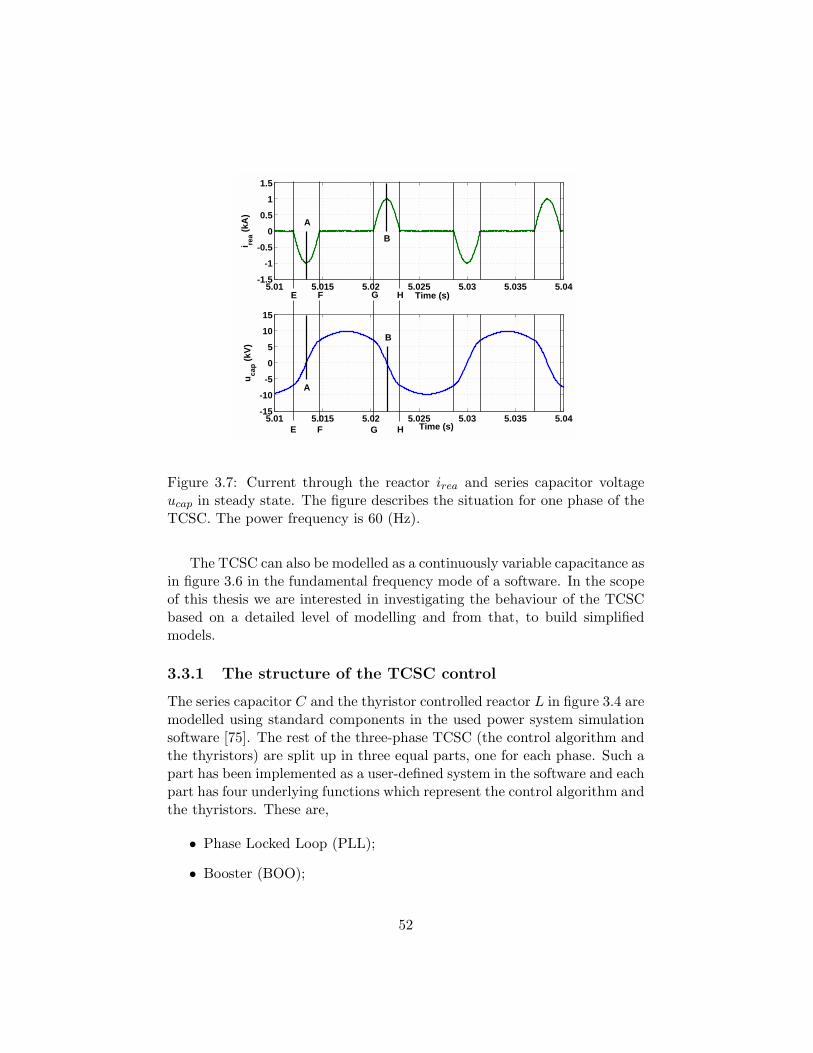
5.01 5.015 5.02 5.025 5.03 5.035 5.04-1.5

-1

-0.5

0

0.5

1

1.5

Time (s)

i rea (k

A)

5.01 5.015 5.02 5.025 5.03 5.035 5.04-15

-10

-5

0

5

10

15

Time (s)

u cap (k

V)

E F

E F

A

A

B

B

G H

HG

Figure 3.7: Current through the reactor irea and series capacitor voltageucap in steady state. The figure describes the situation for one phase of theTCSC. The power frequency is 60 (Hz).

The TCSC can also be modelled as a continuously variable capacitance asin figure 3.6 in the fundamental frequency mode of a software. In the scopeof this thesis we are interested in investigating the behaviour of the TCSCbased on a detailed level of modelling and from that, to build simplifiedmodels.

3.3.1 The structure of the TCSC control

The series capacitor C and the thyristor controlled reactor L in figure 3.4 aremodelled using standard components in the used power system simulationsoftware [75]. The rest of the three-phase TCSC (the control algorithm andthe thyristors) are split up in three equal parts, one for each phase. Such apart has been implemented as a user-defined system in the software and eachpart has four underlying functions which represent the control algorithm andthe thyristors. These are,

• Phase Locked Loop (PLL);

• Booster (BOO);

52

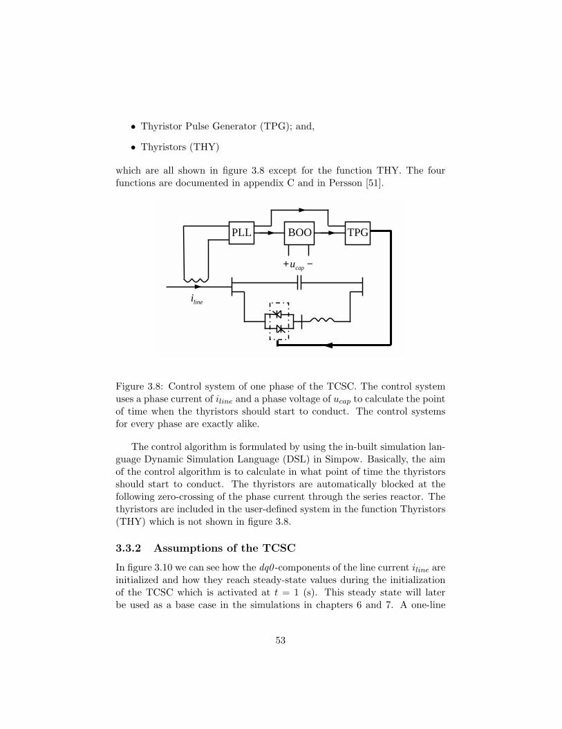
• Thyristor Pulse Generator (TPG); and,

• Thyristors (THY)

which are all shown in figure 3.8 except for the function THY. The fourfunctions are documented in appendix C and in Persson [51].

−+ capu

linei

PLL BOO TPG

Figure 3.8: Control system of one phase of the TCSC. The control systemuses a phase current of iline and a phase voltage of ucap to calculate the pointof time when the thyristors should start to conduct. The control systemsfor every phase are exactly alike.

The control algorithm is formulated by using the in-built simulation lan-guage Dynamic Simulation Language (DSL) in Simpow. Basically, the aimof the control algorithm is to calculate in what point of time the thyristorsshould start to conduct. The thyristors are automatically blocked at thefollowing zero-crossing of the phase current through the series reactor. Thethyristors are included in the user-defined system in the function Thyristors(THY) which is not shown in figure 3.8.

3.3.2 Assumptions of the TCSC

In figure 3.10 we can see how the dq0 -components of the line current iline areinitialized and how they reach steady-state values during the initializationof the TCSC which is activated at t = 1 (s). This steady state will laterbe used as a base case in the simulations in chapters 6 and 7. A one-line

53

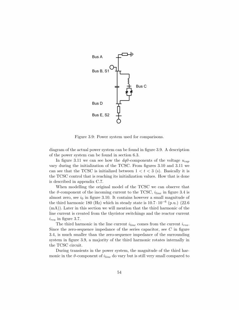
Bus A

Bus B, S1

Bus D

Bus E, S2

Bus C

Figure 3.9: Power system used for comparisons.

diagram of the actual power system can be found in figure 3.9. A descriptionof the power system can be found in section 6.3.

In figure 3.11 we can see how the dq0 -components of the voltage ucap

vary during the initialization of the TCSC. From figures 3.10 and 3.11 wecan see that the TCSC is initialized between 1 < t < 3 (s). Basically it isthe TCSC control that is reaching its initialization values. How that is doneis described in appendix C.7.

When modelling the original model of the TCSC we can observe thatthe 0 -component of the incoming current to the TCSC, iline in figure 3.4 isalmost zero, see i0 in figure 3.10. It contains however a small magnitude ofthe third harmonic 180 (Hz) which in steady state is 10.7 · 10−6 (p.u.) (22.6(mA)). Later in this section we will mention that the third harmonic of theline current is created from the thyristor switchings and the reactor currentirea in figure 3.7.

The third harmonic in the line current iline comes from the current irea.Since the zero-sequence impedance of the series capacitor, see C in figure3.4, is much smaller than the zero-sequence impedance of the surroundingsystem in figure 3.9, a majority of the third harmonic rotates internally inthe TCSC circuit.

During transients in the power system, the magnitude of the third har-monic in the 0 -component of iline do vary but is still very small compared to

54

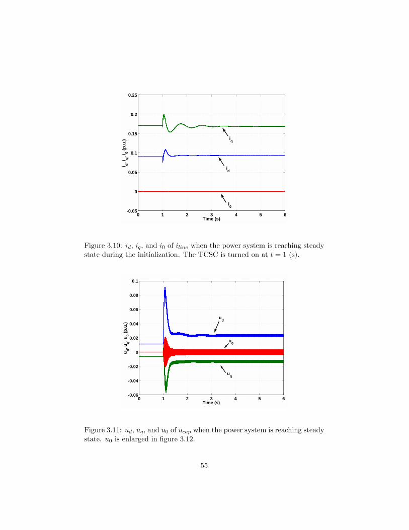
0 1 2 3 4 5 6-0.05

0

0.05

0.1

0.15

0.2

0.25

Time (s)

i d, iq, i

0 (p.u

.)

id

iq

i0

Figure 3.10: id, iq, and i0 of iline when the power system is reaching steadystate during the initialization. The TCSC is turned on at t = 1 (s).

0 1 2 3 4 5 6-0.06

-0.04

-0.02

0

0.02

0.04

0.06

0.08

0.1

Time (s)

u d, uq, u

0 (p.u

.)

ud

u0

uq

Figure 3.11: ud, uq, and u0 of ucap when the power system is reaching steadystate. u0 is enlarged in figure 3.12.

55

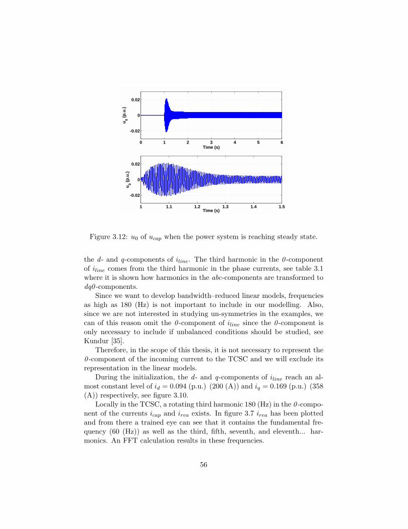
0 1 2 3 4 5 6

-0.02

0

0.02

Time (s)

u 0 (p.u

.)

1 1.1 1.2 1.3 1.4 1.5

-0.02

0

0.02

Time (s)

u 0 (p.u

.)

Figure 3.12: u0 of ucap when the power system is reaching steady state.

the d - and q-components of iline. The third harmonic in the 0 -componentof iline comes from the third harmonic in the phase currents, see table 3.1where it is shown how harmonics in the abc-components are transformed todq0 -components.

Since we want to develop bandwidth–reduced linear models, frequenciesas high as 180 (Hz) is not important to include in our modelling. Also,since we are not interested in studying un-symmetries in the examples, wecan of this reason omit the 0 -component of iline since the 0 -component isonly necessary to include if unbalanced conditions should be studied, seeKundur [35].

Therefore, in the scope of this thesis, it is not necessary to represent the0 -component of the incoming current to the TCSC and we will exclude itsrepresentation in the linear models.

During the initialization, the d - and q-components of iline reach an al-most constant level of id = 0.094 (p.u.) (200 (A)) and iq = 0.169 (p.u.) (358(A)) respectively, see figure 3.10.

Locally in the TCSC, a rotating third harmonic 180 (Hz) in the 0 -compo-nent of the currents icap and irea exists. In figure 3.7 irea has been plottedand from there a trained eye can see that it contains the fundamental fre-quency (60 (Hz)) as well as the third, fifth, seventh, and eleventh... har-monics. An FFT calculation results in these frequencies.

56

In steady state the frequency component for the third harmonic createsthe same magnitude and phase within all three phases and since the 0 -component is defined as with equation (3.1); the 0 -component is equal tothe sum of the three phases multiplied with a factor of 1

3 .The third harmonic in the local TCSC current causes a third harmonic

in the 0 -component of the voltage drop ucap over C, see figure 3.12. It canbe shown that if the magnitude of a third harmonic is M3 with the samephase in all three phase voltages (as in our steady-state case), then we willget the same magnitude M3 of the third harmonic in the 0 -component ofucap. This is shown in table 3.1 and in figure 3.13. In the upper part offigure 3.13 we can see that we have 0.0036 (p.u.) of the third harmonic180 (Hz) in all three phases and in the lower part of the figure we have thesame magnitude of the third harmonic 180 (Hz) in the 0 -component. The0 -component is the red graph in the back in the lower part of figure 3.13.Observe that the scales are not equal in the upper and lower parts of thefigure.

However, such a high frequency is not interesting when describing thelow-frequency behavior of the TCSC and therefore also the 0 -component ofthe voltage drop ucap is omitted in the linear model of the TCSC.

Table 3.1 shows how existing harmonics in the three-phase voltages abcappears in the corresponding dq0 -components. Observe that both 300 (Hz)and 420 (Hz) in the phase voltages abc appear as 360 (Hz) in the d - andq-components.

In the table it has been assumed that an harmonic appear with the samemagnitude in all three phases.

In figure 3.13, |M3| is 13.5% of |M1|, |M5| is 5.1% of |M1|, |M7| is 1.5%of |M1|, |M11| is 0.4% of |M1|, and |M13| is 0.3% of |M1|.

In table 3.1 the fundamental frequency (60 Hz) is symmetric in the threephases, i.e., with forward phase order and 120 phase difference and withthe same magnitude in all phases.

The third harmonic (180 Hz) has no phase difference, i.e., 0 phasedifference. The fifth harmonic (300 Hz) and eleventh harmonic (660 Hz)appear with reverse phase order and 120 phase difference. The seventh (420Hz) and thirteenth harmonic (780 Hz) appear with forward phase order and120 phase difference.

The constant k in table 3.1 is a scalar with a value between zero andone. The results in table 3.1 have been derived by studying equation (3.1).The results are also summarized in figure 3.13.

Since both the fifth and seventh harmonics in the abc-components areextracted to the same frequency (300 (Hz)) in the dq-components, they can

57

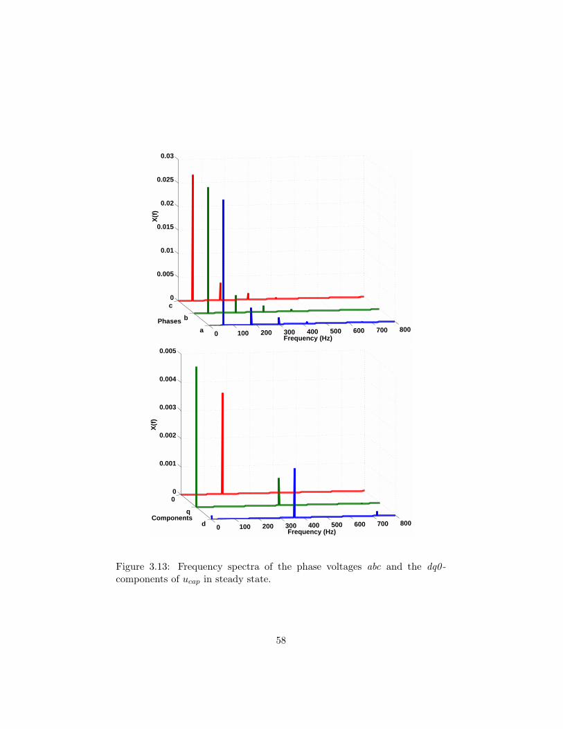
0 100 200 300 400 500 600 700 800a

b

c0

0.005

0.01

0.015

0.02

0.025

0.03

Frequency (Hz)

Phases

X(f

)

0 100 200 300 400 500 600 700 800d

q

00

0.001

0.002

0.003

0.004

0.005

Frequency (Hz)

Components

X(f

)

Figure 3.13: Frequency spectra of the phase voltages abc and the dq0 -components of ucap in steady state.

58

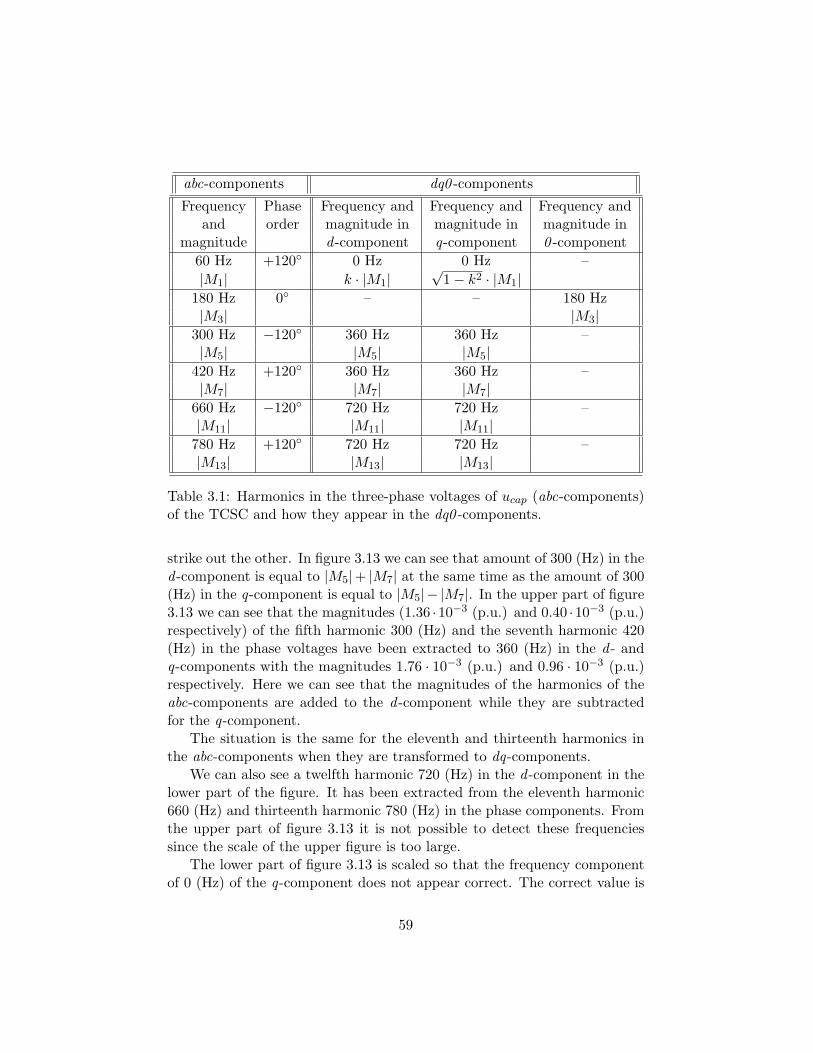
abc-components dq0 -components

Frequency Phase Frequency and Frequency and Frequency andand order magnitude in magnitude in magnitude in

magnitude d -component q-component 0 -component60 Hz +120 0 Hz 0 Hz –|M1| k · |M1|

√1− k2 · |M1|

180 Hz 0 – – 180 Hz|M3| |M3|

300 Hz −120 360 Hz 360 Hz –|M5| |M5| |M5|

420 Hz +120 360 Hz 360 Hz –|M7| |M7| |M7|

660 Hz −120 720 Hz 720 Hz –|M11| |M11| |M11|

780 Hz +120 720 Hz 720 Hz –|M13| |M13| |M13|

Table 3.1: Harmonics in the three-phase voltages of ucap (abc-components)of the TCSC and how they appear in the dq0 -components.

strike out the other. In figure 3.13 we can see that amount of 300 (Hz) in thed -component is equal to |M5|+ |M7| at the same time as the amount of 300(Hz) in the q-component is equal to |M5|− |M7|. In the upper part of figure3.13 we can see that the magnitudes (1.36 ·10−3 (p.u.) and 0.40 ·10−3 (p.u.)respectively) of the fifth harmonic 300 (Hz) and the seventh harmonic 420(Hz) in the phase voltages have been extracted to 360 (Hz) in the d - andq-components with the magnitudes 1.76 · 10−3 (p.u.) and 0.96 · 10−3 (p.u.)respectively. Here we can see that the magnitudes of the harmonics of theabc-components are added to the d -component while they are subtractedfor the q-component.

The situation is the same for the eleventh and thirteenth harmonics inthe abc-components when they are transformed to dq-components.

We can also see a twelfth harmonic 720 (Hz) in the d -component in thelower part of the figure. It has been extracted from the eleventh harmonic660 (Hz) and thirteenth harmonic 780 (Hz) in the phase components. Fromthe upper part of figure 3.13 it is not possible to detect these frequenciessince the scale of the upper figure is too large.

The lower part of figure 3.13 is scaled so that the frequency componentof 0 (Hz) of the q-component does not appear correct. The correct value is

59

0.0267 (p.u.) which is higher than the maximum value of the y-axis in thefigure.

3.4 Use of filter to remove harmonics

In section 3.3.2 it has been shown from where the harmonics in the dq0 -components are derived. We could see that in the d - and q-components wehave 360 and 720 (Hz) during normal conditions. The amount of 360 (Hz)in the d - and q-components appeared from the fifth 300 (Hz) and seventhharmonic 420 (Hz) in the three phase voltages abc.

In this work the harmonics are not of interest since we want to createmodels of the TCSC which represent its slow behavior. Later we will there-fore low-pass filter the d - and q-components to enable focusing on the slowbehavior of the component. The used low-pass filter has the characteristicas shown in figure 3.14.

10-1

100

101

102

103

-40

-30

-20

-10

0Bode Diagram

Mag

nitu

de (d

B)

10-1

100

101

102

103

-80

-60

-40

-20

0

Pha

se (d

eg)

Frequency (Hz)

Figure 3.14: Frequency characteristic for the used low-pass filter.

The used low-pass filter is a first-order filter,

H(s) =1

1 + sT. (3.9)

For our study object we have filtered the voltages ud and uq with the

60

filter constant T = 0.01 (s). The time constant T = 0.01 (s) gives a 3 (dB)bandwidth at 15.9 (Hz).

3.5 The accuracy of the model of the Thyristor-Controlled Series Capacitor

The TCSC model in the thesis has been developed with the support fromABB, Angquist [87] and it follows the Synchronous Voltage Reversal-controlalgorithm developed by ABB, see Angquist [88, 89]. Through the develop-ment of the model the aim has been to derive a TCSC model that worksand is representative for a TCSC. The aim has not been to model an exactexisting physical installation of a TCSC although the here developed modelis influenced from existing TCSC installations. The aim of the developedTCSC model is to represent a study object in the thesis to which we applydifferent ideas of simplifying the modelling when developing linear models.

Whether the model is representing an existing real TCSC model is notinvestigated in the thesis. However, the functionality of the TCSC modelcovers the fundamentals of a TCSC.

3.6 Summary

In this chapter some formulations and fundamentals of the modelling of thepower system in the thesis has been mentioned. In the chapter it has beenexplained both the modelling of the power system as well as comments aboutspecific models that are simulated in the thesis. Also the modelling of theoriginal TCSC model have been outlined.

61

62

Chapter 4

Developing linear models

In this chapter it is generally described how to develop simplified linear mod-els of a system. It contains discussions of different methods when linearizinga power system containing the non-linear power system component TCSC.It also includes the processes of how the linear models for our study object,the TCSC, are created.

4.1 Introduction

When developing a model of an existing system it can be done with knowl-edge about the physical system and to investigate the physical system tobuild a model.

One problem that might occur is how to set numerical values of theparameters in the model? Hopefully some of the parameters are documentedin data sheets of the physical system. This process can be complicated if itis necessary to derive the dynamics for the real system that might have acomplex structure.

To overcome problems as mentioned above it can be easier to use mea-surements of the system. By sending a well-defined input signal into thesystem and record the output signal from it, it is possible to analyze thesystem. In that analysis it is possible to identify the dynamical responseof the system, for instance its transfer function(s). That process is calledsystem identification, Schmidtbauer [74].

In other words, instead of trying to get a known output signal by tryingto build a model from the physical relations of the system we in systemidentification try to do it in the opposite way; to use the input and outputsignals and with that knowledge create a system, without including the

63

physical relations of the system (to treat the system as a black box ).In this work we have made the system identification both in the time

domain as well as in the frequency domain. We have used the following twotechniques,

• Transient Analysis, i.e., in a time-domain simulation disturb input byinput from a steady-state situation; and

• Frequency Analysis, i.e., in a time-domain simulation from a steady-state situation disturb input by input with sinus-formed signals ofvarying frequencies.

One difference between the two techniques is that the measurementswith the frequency analysis demands longer simulation time since the systemshould be excited with a number of input signals of different frequencies.

A general list of how to structure an identification work is listed below.Both general comments are given as well as specific comments for our studyobject.

i) A component and its state

There are different reasons for identifying a simplified model for acomponent. One reason can be its high complexity or that it has tobe simplified to fit in the actual modelling possibilities for a certainsoftware. The component might be operated in different states, withdifferent behavior that can be hard to represent in the software. Whenidentifying the model it is necessary to decide which state the modelshould be valid for.

In our case the study object is a TCSC with a certain control algo-rithm. The state of the TCSC in the thesis is restricted only to itscapacitive region.

This point has a connection to point ii in the list.

ii) Do pre-studies

Is it meaningful to build a linear model? It is recommended to dosome pre-studies to control if the component has the possibility to berepresented by a linear model. These investigations should representnormal conditions that we later want to simulate with the linear model.

In sections 4.4 – 4.6 such pre-studies of our study object are found.

64

iii) Preparation of signals – Select bandwidth

Before starting the identification process of a model it might be neces-sary to prepare the signals. It can be for instance to analyze the noisethat can be included in the input signals. The aim of the identifiedmodel influence this point. It has to be clear what the aim of thestudies are. Is it a model that should represent a certain bandwidth?

For our study object the focus have been to represent frequencies upto some Hertz.

The obtained models consist of two parts, one part which represent thesteady-state part of the component and another part which representthe dynamic behavior of the component.

iv) Choose input and output signals

To select input and output signals for a component demands knowledgeabout the studied component.

After studies documented in section 3.3.2 we have decided to representthe linear models of our study object with two input signals (currentsid and iq) and two output signals (voltages ud and uq).

v) Choose environment

The environment should be easy to analyze. A simple understandableenvironment makes the response in the studied component easy andclear to understand. To select environment for a component demandsknowledge about it and its response for certain scenarios.

In this work we have used two different environments. One for identi-fying the linear models and another to investigate their validity.

vi) Identification methods

In sections 4.7 and 4.8 the two identification processes used in thisthesis can be found.

vii) Validation

The obtained linear models have to be validated. For instance, toexamine their properties towards the original models.

In Ljung [41] basic steps of system identification can be found includingsimilar points as above.

65

4.2 Different methodologies

In this section we discuss earlier published methods when linearizing a powersystem containing a TCSC.

4.2.1 Poincare map

In Jalali [23, 26], state space analysis of circuits containing Thyristor Con-trolled Reactors (TCRs) have been applied. The Poincare map has beenused to study the non-linear dynamics of different TCR circuits. It hasbeen shown that a TCR circuit can damp small perturbations even whenthe resistances of the TCR circuit are ignored and the thyristors are assumedto be ideal.

In Jalali [23, 26] the installed Kayenta Substation controller of a TCSCin northeastern Arizona, USA (see Christl [7, 8]) has been studied. It isin Jalali [23, 26] stated that the dynamic response of a TCSC changes asa function of the thyristor conduction time σ. This dependence is alsodiscussed in other papers describing the design of the Kayenta system, seefor instance Christl [7, 8].

In Jalali [26] it is shown that the dynamics of the TCSC depends on theTCSC’s conduction time σ during steady state in the operating point. Byusing the Jacobian of the Poincare map it is in Jalali [26] possible to analyzethe small-signal stability of the system. The eigenvalues of the system inJalali [26] are shown in the unit circle.

The TCSC model in Jalali [26] does not represent the impact of the linecurrent on the TCSC voltage and does not have the capability to repre-sent the synchronization system or the higher-level control loops, see Oth-man [48].

The Poincare map have also been used in Dobson [11] and Othman [48].

4.2.2 Identification from Bode plots

In Christl [8] the design of the Kayenta controller of a TCSC was achievedby first finding the open loop response of line current to changes in thefiring point using a detailed EMTP model. The resulting envelope of theline current response enabled control engineers to find a transfer functionwhich approximates the dynamics of the system around an operating point.The resulting fourth order transfer function has two poles on the real axisand a complex pair of poles. The dependence of the complex poles on the

66

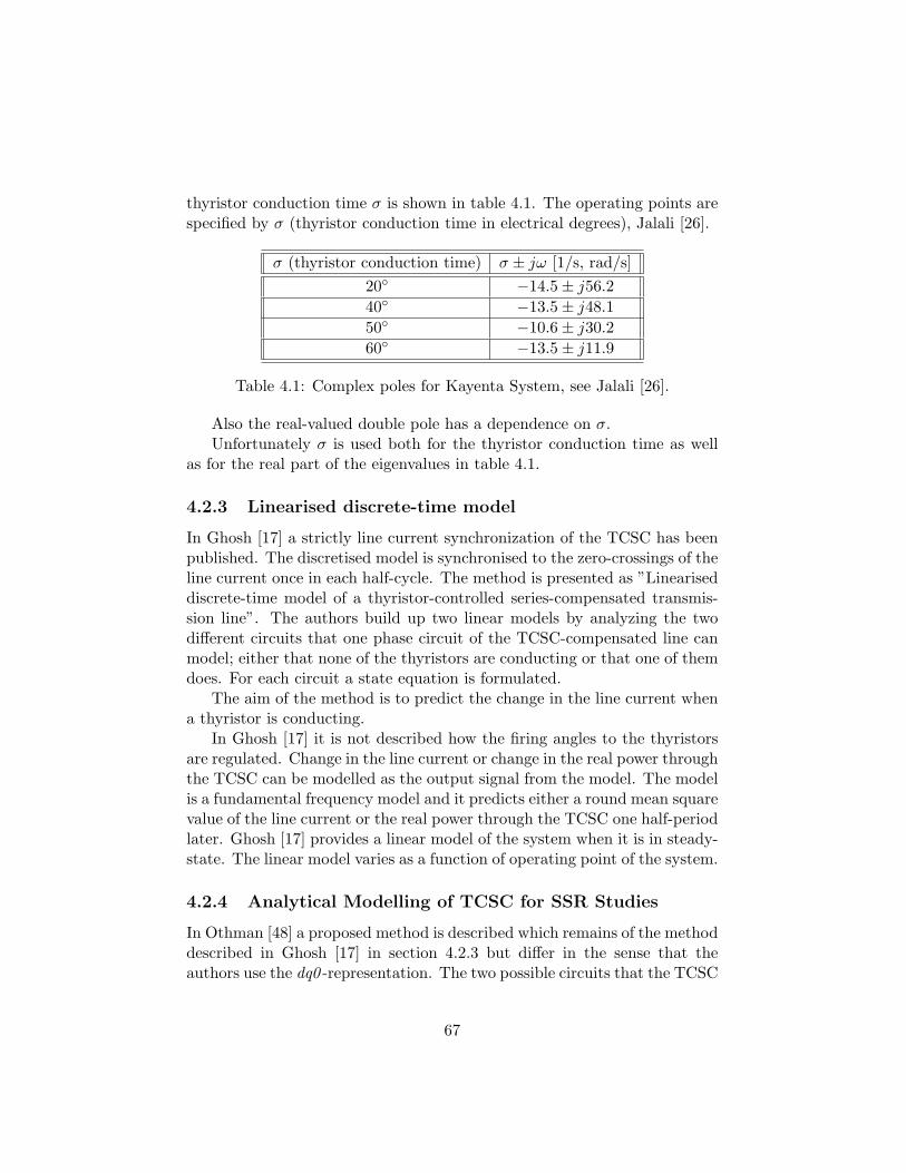
thyristor conduction time σ is shown in table 4.1. The operating points arespecified by σ (thyristor conduction time in electrical degrees), Jalali [26].

σ (thyristor conduction time) σ ± jω [1/s, rad/s]20 −14.5± j56.240 −13.5± j48.150 −10.6± j30.260 −13.5± j11.9

Table 4.1: Complex poles for Kayenta System, see Jalali [26].

Also the real-valued double pole has a dependence on σ.Unfortunately σ is used both for the thyristor conduction time as well

as for the real part of the eigenvalues in table 4.1.

4.2.3 Linearised discrete-time model

In Ghosh [17] a strictly line current synchronization of the TCSC has beenpublished. The discretised model is synchronised to the zero-crossings of theline current once in each half-cycle. The method is presented as ”Lineariseddiscrete-time model of a thyristor-controlled series-compensated transmis-sion line”. The authors build up two linear models by analyzing the twodifferent circuits that one phase circuit of the TCSC-compensated line canmodel; either that none of the thyristors are conducting or that one of themdoes. For each circuit a state equation is formulated.

The aim of the method is to predict the change in the line current whena thyristor is conducting.

In Ghosh [17] it is not described how the firing angles to the thyristorsare regulated. Change in the line current or change in the real power throughthe TCSC can be modelled as the output signal from the model. The modelis a fundamental frequency model and it predicts either a round mean squarevalue of the line current or the real power through the TCSC one half-periodlater. Ghosh [17] provides a linear model of the system when it is in steady-state. The linear model varies as a function of operating point of the system.

4.2.4 Analytical Modelling of TCSC for SSR Studies

In Othman [48] a proposed method is described which remains of the methoddescribed in Ghosh [17] in section 4.2.3 but differ in the sense that theauthors use the dq0 -representation. The two possible circuits that the TCSC

67

can represent in one phase are described. The model is valid in the frequencyrange from 0 (Hz) to twice the operating frequency.

The inputs to the TCSC model are the capacitor voltage at the presentinstant t0, the dq0 -components of the line current, and the upcoming thyris-tor triggering instant φ1/2, see figure 4.1. The output of the TCSC modelis the capacitor voltage one half cycle later from time t0 at time t1/2, seefigure 4.1.

2.2 2.21 2.22 2.23 2.24 2.25-0.8

-0.6

-0.4

-0.2

0

0.2

0.4

0.6

Time (s)

I line, I

thyr

(p.

u.)

t0 t

1/2

τ1/2

φ1/2

Iline Ithyr

Figure 4.1: One phase line current iline and an associated thyristor currentithyr (earlier introduced as irea).

The obtained linearized model is dependent on the thyristor-triggeringinstant φ1/2 and the operating point.

The analytical linearized model of the single-phase TCSC seeks to predictthe changes in the capacitor voltage at time t1/2 from its equilibrium value.The value of the capacitor voltage at t1/2 is a function of the change in thecapacitor voltage at time t0, the change in the thyristor triggering instantφ1/2, and the change in the line current during the half cycle between t0 andt1/2.

Later, the single-phase model of the TCSC is expanded straightforwardto a three-phase model assuming that the line current is symmetric and thatthe thyristor triggering instants are equally spaced for the three phases withπ3 (rad), i.e., 1

6 of the fundamental period.

68

4.2.5 Phasor Dynamics

Models have been derived using a general averaging theory for converterswitching circuits in Mattavelli [46]. These models are based on formingdynamical equations, which describe the development of the essential Fouriercomponents that characterize the operation of the TCSC. One assumptionof Mattavelli [46] is that the line current is essentially sinusoidal.

The method Phasor Dynamics develops a continuous-time model for theTCSC. The model is based on a representation of voltages and currents astime-varying Fourier coefficients. The Fourier coefficients (Fourier series)are truncated to keep only the fundamental component of it.

Mattavelli [46] derives a TCSC model based on time-varying Fourier co-efficients that capture the phasor dynamics of the TCSC. The approach canbe viewed as intermediate between instantaneous value mode and the quasi-static sinusoidal steady-state approximation. The TCSC’s phasor dynamicsrepresent the dynamics of the fundamental currents and voltages. The de-veloped model of the TCSC is a phasor model of fourth-order. The modelcan be linearized and in different operating points it provides different linearmodels.

4.2.6 Prony Analysis

In Dolan [13] an application of Prony analysis is shown when identifying aTCSC system of Slatt 500 kV substation, Arlington Oregon, USA.

Dolan [13] shows good result for closed loop identification but these areonly accurate for small variations near the operating point used for theidentification of the system.

4.2.7 Discrete-time model

In Jalali [25] a method is presented to create a stability model of a TCSCto be used in time-domain simulations. The purpose of the stability modelis to correctly represent the fundamental component of the series capacitorvoltage for line currents which contain variation in both magnitude andphase. The stability model is essentially the solution to the differentialequations of the TCSC circuit. It updates the capacitor voltage every half-cycle based on the line current, the thyristor firing time and the initialcapacitor voltage and is therefore a discrete-time model. The TCSC circuit isobtained by representing the thyristor valve by an equivalent current source.By introducing an internal state variable to keep track of the capacitorvoltage, a discrete-time equation for the current in this equivalent source is

69

formulated. The range of frequencies is limited to power swing values of 0.1to 3.0 (Hz). The model is tested in a small power system consisting of atransmission line, a TCSC, an infinite bus, and a classical representation ofa synchronous machine.

The method can only be implemented into stability programs whichutilize a fixed time step integration routine.

4.2.8 State-space model depending on the firing angle

In Jovcic [29] a second order transfer function is identified using frequencyresponse (frequency analysis) to represent the TCSC. The characteristicfrequency of the denominator has a linear relationship with the firing angle.

4.2.9 Summary of different methodologies

In sections 4.2.1 – 4.2.8 different methods in the literature with the aim tobuild simplified models of a TCSC, have been listed.

In Christl [8] a fourth-order linear model identified from Bode Plots(frequency analysis) was derived. The poles of the model were dependent onthe thyristor conduction angle σ. Time-domain comparisons showed goodagreement between the identified model and the original detailed model.Also in Jovcic [29] a linear model (of second order) was identified by usingfrequency analysis.

In Jalali [26] a fourth-order linear model have been developed but hereit has been done by analyzing the circuit of the TCSC and applying thePoincare map.

Also in Ghosh [17], Othman [48], Mattavelli [46], and Jalali [25] thecircuit of the TCSC is analyzed in order to build a linear model.

In Dolan [13] identification of a TCSC have been done with transientanalysis by using Prony analysis.

Contribution from this work

Compared to previous studies, this thesis contains development of two linearmodels with transient and frequency analysis from a detailed TCSC model.As mentioned above, similar works have been reported in Christl [8], Jov-cic [29] and Dolan [13]. In Christl [8] and Jovcic [29] the identificationprocess is not documented and in Dolan [13] the transient analysis is doneusing Prony Analysis. In this work the identification processes are well-documented. In the identification processes we have treated the study ob-

70

ject as a black box, i.e., we have not analyzed the circuit of the TCSC tobuild linear models.

The developed models have been investigated in time-domain simulationsand small-signal stability analysis.

4.3 Introduction to linearization of the TCSC

In the thesis we have modelled a detailed original model of a TCSC of whichwe build simplified linear models. The original TCSC model including asmall surrounding power system contains in total 69 state variables of whichthe original TCSC model contains 22. The state variables of the originalTCSC model are for instance variables of the control algorithm described inappendix C.

The created simplified models are abstract linear models that shouldrepresent the detailed original model of the TCSC although they are lim-ited in bandwidth. The state variables in the created linear models do notrepresent real physical quantities such as measurable angles and voltages,instead they are representing abstract quantities.

To create the linear models we study the response of the original TCSCmodel by disturbing it with well-defined input signals. Then we record theoutput signals which we use for developing linear models. We will developthe linear models with two techniques namely,

• transient analysis, i.e., in a time-domain simulation disturb the inputswith a step in a steady-state situation; and

• frequency analysis, i.e., in a time-domain simulation of a steady-statesituation disturb the inputs with sinus-formed signals with constantamplitude and varying frequencies.

In both items above we record the output signals from the model andidentify the TCSC with the two techniques.

The task in this chapter is to describe the behavior of a physical compo-nent and investigate whether it is possible to simplify its representation witha linear model and in that case how that model should look like. A physicalcomponent consists of several interactive parts and is therefore representedas a ”system” below. In the following we will step by step motivate ourprogress in this process.

Let us say that we have a system containing p input signals u1, . . . ,up and m output signals y1, . . . , ym as shown in figure 4.2.

71

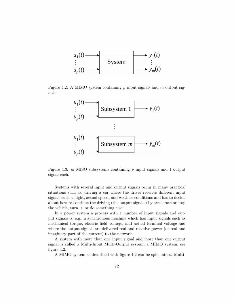
u1(t)

up(t)System

… y1(t)…

ym(t)

Figure 4.2: A MIMO system containing p input signals and m output sig-nals.

u1(t)

up(t)Subsystem 1

… y1(t)

…

u1(t)

up(t)Subsystem m

… ym(t)

Figure 4.3: m MISO subsystems containing p input signals and 1 outputsignal each.

Systems with several input and output signals occur in many practicalsituations such as; driving a car where the driver receives different inputsignals such as light, actual speed, and weather conditions and has to decideabout how to continue the driving (the output signals) by accelerate or stopthe vehicle, turn it, or do something else.

In a power system a process with a number of input signals and out-put signals is, e.g., a synchronous machine which has input signals such asmechanical torque, electric field voltage, and actual terminal voltage andwhere the output signals are delivered real and reactive power (or real andimaginary part of the current) to the network.

A system with more than one input signal and more than one outputsignal is called a Multi-Input Multi-Output system, a MIMO system, seefigure 4.2.

A MIMO system as described with figure 4.2 can be split into m Multi-

72

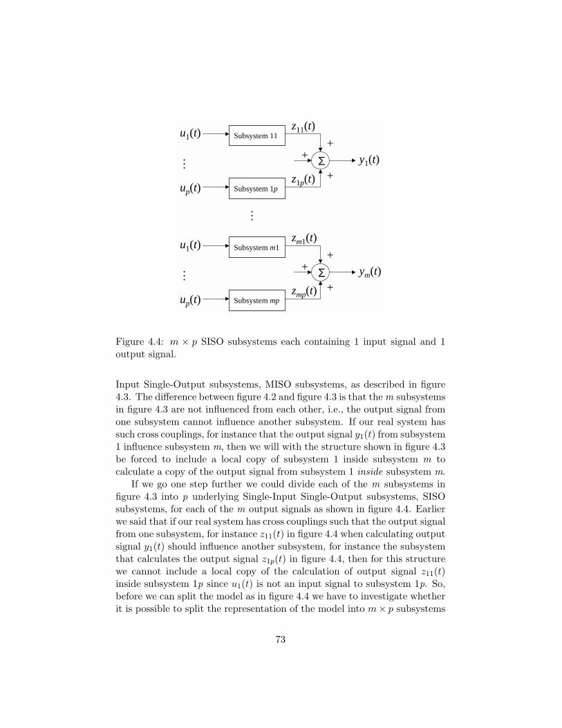
u1(t)

up(t)

… y1(t)Σ

Subsystem 11+

Subsystem 1p+

+

u1(t)

up(t)

… ym(t)Σ

Subsystem m1+

Subsystem mp+

+

…

z11(t)

z1p(t)

zmp(t)

zm1(t)

Figure 4.4: m × p SISO subsystems each containing 1 input signal and 1output signal.

Input Single-Output subsystems, MISO subsystems, as described in figure4.3. The difference between figure 4.2 and figure 4.3 is that the m subsystemsin figure 4.3 are not influenced from each other, i.e., the output signal fromone subsystem cannot influence another subsystem. If our real system hassuch cross couplings, for instance that the output signal y1(t) from subsystem1 influence subsystem m, then we will with the structure shown in figure 4.3be forced to include a local copy of subsystem 1 inside subsystem m tocalculate a copy of the output signal from subsystem 1 inside subsystem m.

If we go one step further we could divide each of the m subsystems infigure 4.3 into p underlying Single-Input Single-Output subsystems, SISOsubsystems, for each of the m output signals as shown in figure 4.4. Earlierwe said that if our real system has cross couplings such that the output signalfrom one subsystem, for instance z11(t) in figure 4.4 when calculating outputsignal y1(t) should influence another subsystem, for instance the subsystemthat calculates the output signal z1p(t) in figure 4.4, then for this structurewe cannot include a local copy of the calculation of output signal z11(t)inside subsystem 1p since u1(t) is not an input signal to subsystem 1p. So,before we can split the model as in figure 4.4 we have to investigate whetherit is possible to split the representation of the model into m× p subsystems

73

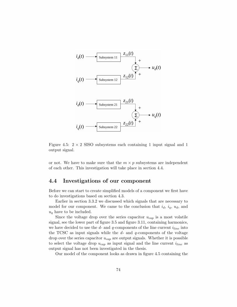
id(t)

iq(t)

ud(t)Σ

Subsystem 11+

Subsystem 12+

id(t)

iq(t)

uq(t)Σ

Subsystem 21+

Subsystem 22+

z11(t)

z12(t)

z22(t)

z21(t)

Figure 4.5: 2 × 2 SISO subsystems each containing 1 input signal and 1output signal.

or not. We have to make sure that the m × p subsystems are independentof each other. This investigation will take place in section 4.4.

4.4 Investigations of our component

Before we can start to create simplified models of a component we first haveto do investigations based on section 4.3.

Earlier in section 3.3.2 we discussed which signals that are necessary tomodel for our component. We came to the conclusion that id, iq, ud, anduq have to be included.

Since the voltage drop over the series capacitor ucap is a most volatilesignal, see the lower part of figure 3.5 and figure 3.11, containing harmonics,we have decided to use the d - and q-components of the line current iline intothe TCSC as input signals while the d - and q-components of the voltagedrop over the series capacitor ucap are output signals. Whether it is possibleto select the voltage drop ucap as input signal and the line current iline asoutput signal has not been investigated in the thesis.

Our model of the component looks as drawn in figure 4.5 containing the

74

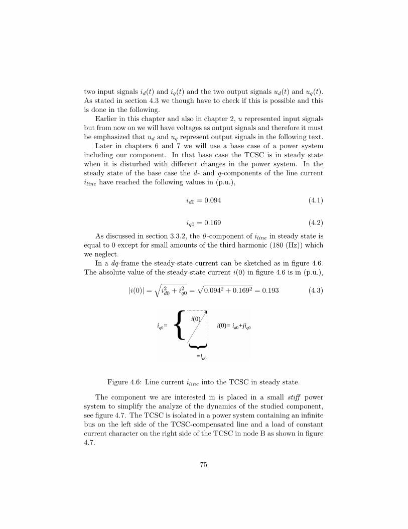
two input signals id(t) and iq(t) and the two output signals ud(t) and uq(t).As stated in section 4.3 we though have to check if this is possible and thisis done in the following.

Earlier in this chapter and also in chapter 2, u represented input signalsbut from now on we will have voltages as output signals and therefore it mustbe emphasized that ud and uq represent output signals in the following text.

Later in chapters 6 and 7 we will use a base case of a power systemincluding our component. In that base case the TCSC is in steady statewhen it is disturbed with different changes in the power system. In thesteady state of the base case the d - and q-components of the line currentiline have reached the following values in (p.u.),

id0 = 0.094 (4.1)

iq0 = 0.169 (4.2)

As discussed in section 3.3.2, the 0 -component of iline in steady state isequal to 0 except for small amounts of the third harmonic (180 (Hz)) whichwe neglect.

In a dq-frame the steady-state current can be sketched as in figure 4.6.The absolute value of the steady-state current i(0) in figure 4.6 is in (p.u.),

|i(0)| =√

i2d0 + i2q0 =√

0.0942 + 0.1692 = 0.193 (4.3)

iq0=

=id0

i(0)i(0)= id0+jiq0

Figure 4.6: Line current iline into the TCSC in steady state.

The component we are interested in is placed in a small stiff powersystem to simplify the analyze of the dynamics of the studied component,see figure 4.7. The TCSC is isolated in a power system containing an infinitebus on the left side of the TCSC-compensated line and a load of constantcurrent character on the right side of the TCSC in node B as shown in figure4.7.

75

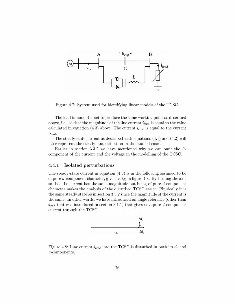
A B+ ucap -

iline C

L

iload∞

Figure 4.7: System used for identifying linear models of the TCSC.

The load in node B is set to produce the same working point as describedabove, i.e., so that the magnitude of the line current iline is equal to the valuecalculated in equation (4.3) above. The current iline is equal to the currentiload.

The steady-state current as described with equations (4.1) and (4.2) willlater represent the steady-state situation in the studied cases.

Earlier in section 3.3.2 we have mentioned why we can omit the 0 -component of the current and the voltage in the modelling of the TCSC.

4.4.1 Isolated perturbations

The steady-state current in equation (4.3) is in the following assumed to beof pure d -component character, given as id0 in figure 4.8. By turning the axisso that the current has the same magnitude but being of pure d -componentcharacter makes the analysis of the disturbed TCSC easier. Physically it isthe same steady state as in section 3.3.2 since the magnitude of the current isthe same. In other words, we have introduced an angle reference (other thanθref that was introduced in section 3.1.1) that gives us a pure d -componentcurrent through the TCSC.

id0 ∆id

∆iq

Figure 4.8: Line current iline into the TCSC is disturbed in both its d - andq-components.

76

It would be possible to let the current be of pure q-component char-acter or a mix of both d - and q-components but here we have selected apure d -component character. Since then, a disturbance in the d -direction isequivalent with a change in the magnitude of the current and a disturbancein the q-direction is equivalent with a change in the angle of the current.

In the stiff power system, the TCSC is perturbed both in the current’sd - and q-component, one by one as in figure 4.8. The load in Node B infigure 4.7 models the load wherein the changes of current takes place.

3 3.5 4 4.5-0.005

0

0.005

0.010

Time (s)

u d (p.u

.)

ud when i

d is perturbed

3 3.5 4 4.5-0.035

-0.030

-0.025

-0.020

-0.015

Time (s)

u q (p.u

.)

uq when i

d is perturbed

3 3.5 4 4.5-0.005

0

0.005

0.010

Time (s)

u d (p.u

.)

ud when i

q is perturbed

3 3.5 4 4.5-0.035

-0.030

-0.025

-0.020

-0.015

Time (s)

u q (p.u

.)

uq when i

q is perturbed

Figure 4.9: Response from the original model of the TCSC when the currenthas been disturbed with a 10%-steps in its d - and q-component.

In figure 4.9 the resulting voltage drop over the series capacitor is plottedwhen the current through the TCSC has been disturbed both in its d - andq-component. The amount of the 6th and 12th harmonics (360 and 720 (Hz)respectively) have been decreased by applying the filter shown in section 3.4.

In the upper part of figure 4.9 the current has been increased with astep of 10% in its d -component. In the upper left corner we can see howthe d -component of the voltage drop ucap responds and in the upper right

77

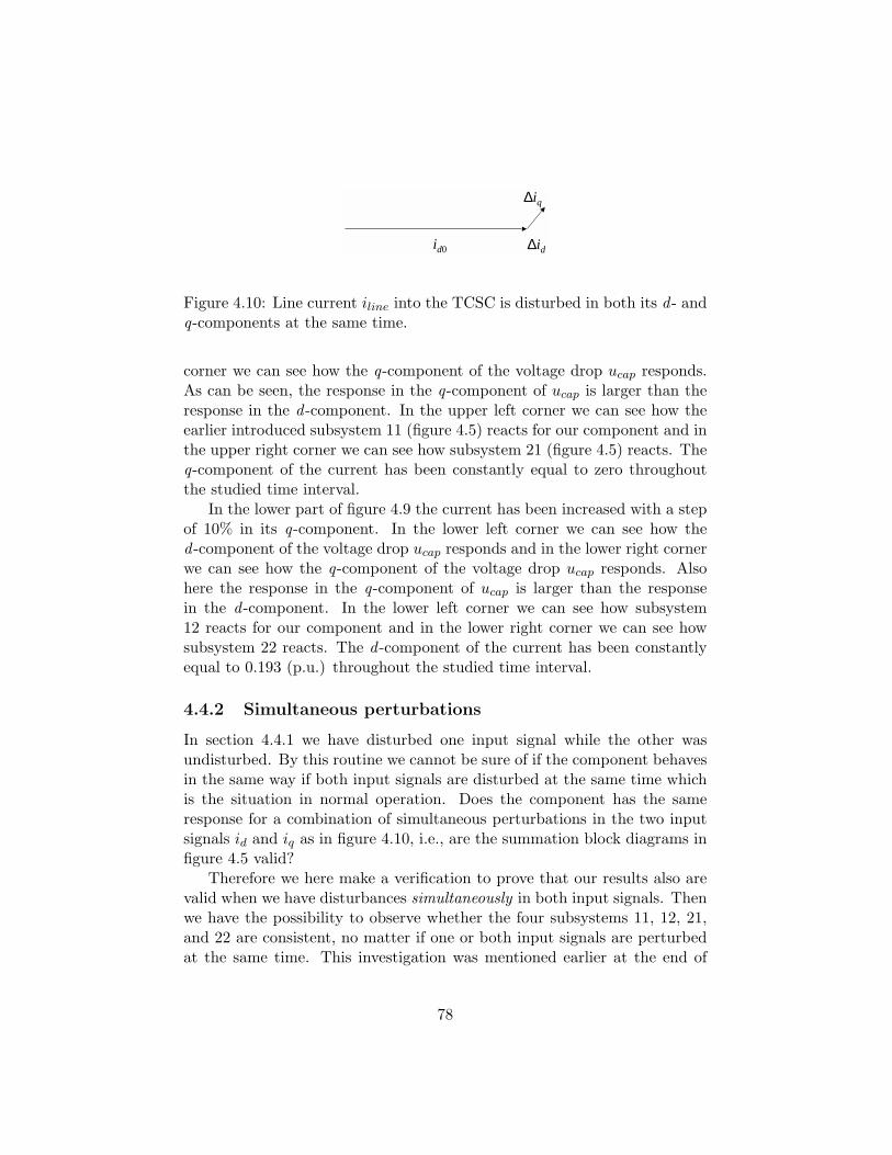
id0 ∆id

∆iq

Figure 4.10: Line current iline into the TCSC is disturbed in both its d - andq-components at the same time.

corner we can see how the q-component of the voltage drop ucap responds.As can be seen, the response in the q-component of ucap is larger than theresponse in the d -component. In the upper left corner we can see how theearlier introduced subsystem 11 (figure 4.5) reacts for our component and inthe upper right corner we can see how subsystem 21 (figure 4.5) reacts. Theq-component of the current has been constantly equal to zero throughoutthe studied time interval.

In the lower part of figure 4.9 the current has been increased with a stepof 10% in its q-component. In the lower left corner we can see how thed -component of the voltage drop ucap responds and in the lower right cornerwe can see how the q-component of the voltage drop ucap responds. Alsohere the response in the q-component of ucap is larger than the responsein the d -component. In the lower left corner we can see how subsystem12 reacts for our component and in the lower right corner we can see howsubsystem 22 reacts. The d -component of the current has been constantlyequal to 0.193 (p.u.) throughout the studied time interval.

4.4.2 Simultaneous perturbations

In section 4.4.1 we have disturbed one input signal while the other wasundisturbed. By this routine we cannot be sure of if the component behavesin the same way if both input signals are disturbed at the same time whichis the situation in normal operation. Does the component has the sameresponse for a combination of simultaneous perturbations in the two inputsignals id and iq as in figure 4.10, i.e., are the summation block diagrams infigure 4.5 valid?

Therefore we here make a verification to prove that our results also arevalid when we have disturbances simultaneously in both input signals. Thenwe have the possibility to observe whether the four subsystems 11, 12, 21,and 22 are consistent, no matter if one or both input signals are perturbedat the same time. This investigation was mentioned earlier at the end of

78

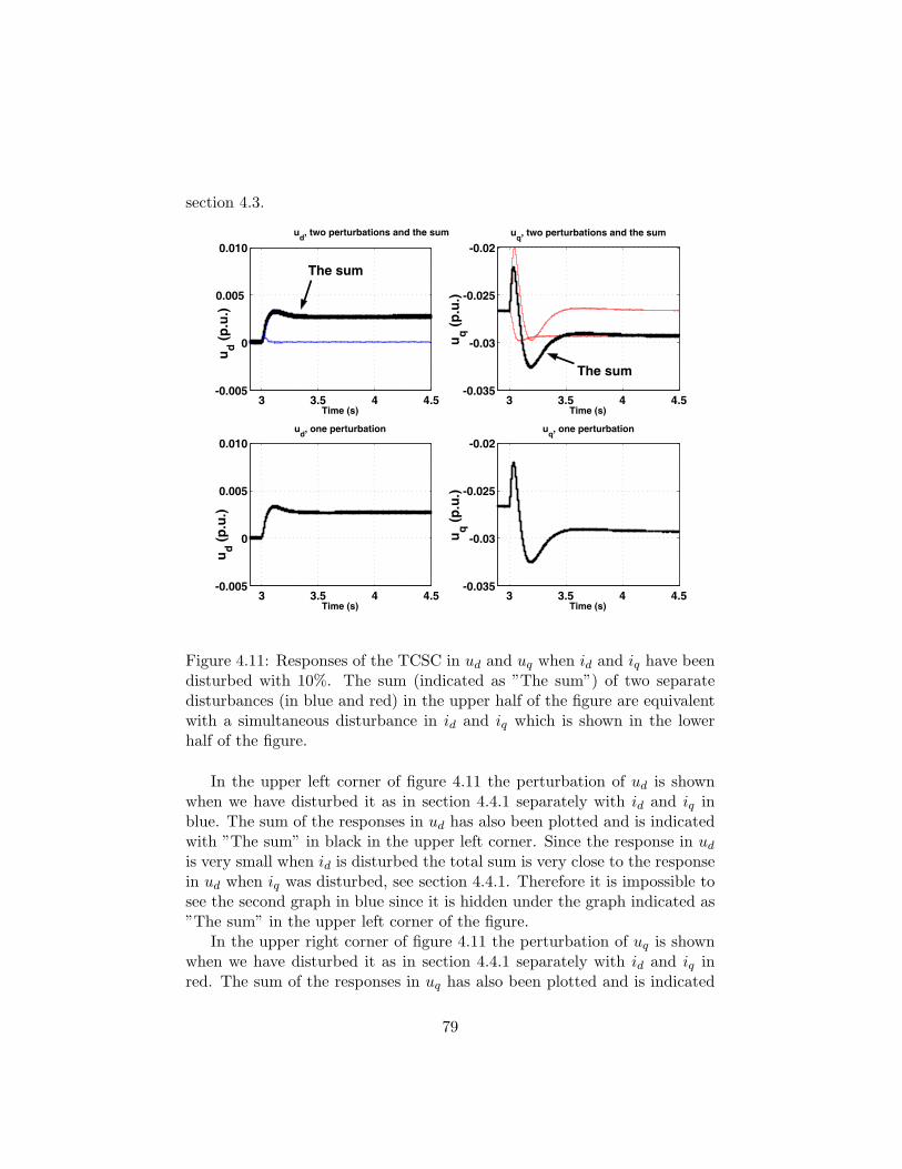
section 4.3.

3 3.5 4 4.5-0.005

0

0.005

0.010

Time (s)

u d (p.u

.)ud, two perturbations and the sum

3 3.5 4 4.5-0.035

-0.03

-0.025

-0.02

Time (s)

u q (p.u

.)

uq, two perturbations and the sum

3 3.5 4 4.5-0.005

0

0.005

0.010

Time (s)

u d (p.u

.)

ud, one perturbation

3 3.5 4 4.5-0.035

-0.03

-0.025

-0.02

Time (s)

u q (p.u

.)

uq, one perturbation

The sum

The sum

Figure 4.11: Responses of the TCSC in ud and uq when id and iq have beendisturbed with 10%. The sum (indicated as ”The sum”) of two separatedisturbances (in blue and red) in the upper half of the figure are equivalentwith a simultaneous disturbance in id and iq which is shown in the lowerhalf of the figure.

In the upper left corner of figure 4.11 the perturbation of ud is shownwhen we have disturbed it as in section 4.4.1 separately with id and iq inblue. The sum of the responses in ud has also been plotted and is indicatedwith ”The sum” in black in the upper left corner. Since the response in ud

is very small when id is disturbed the total sum is very close to the responsein ud when iq was disturbed, see section 4.4.1. Therefore it is impossible tosee the second graph in blue since it is hidden under the graph indicated as”The sum” in the upper left corner of the figure.

In the upper right corner of figure 4.11 the perturbation of uq is shownwhen we have disturbed it as in section 4.4.1 separately with id and iq inred. The sum of the responses in uq has also been plotted and is indicated

79

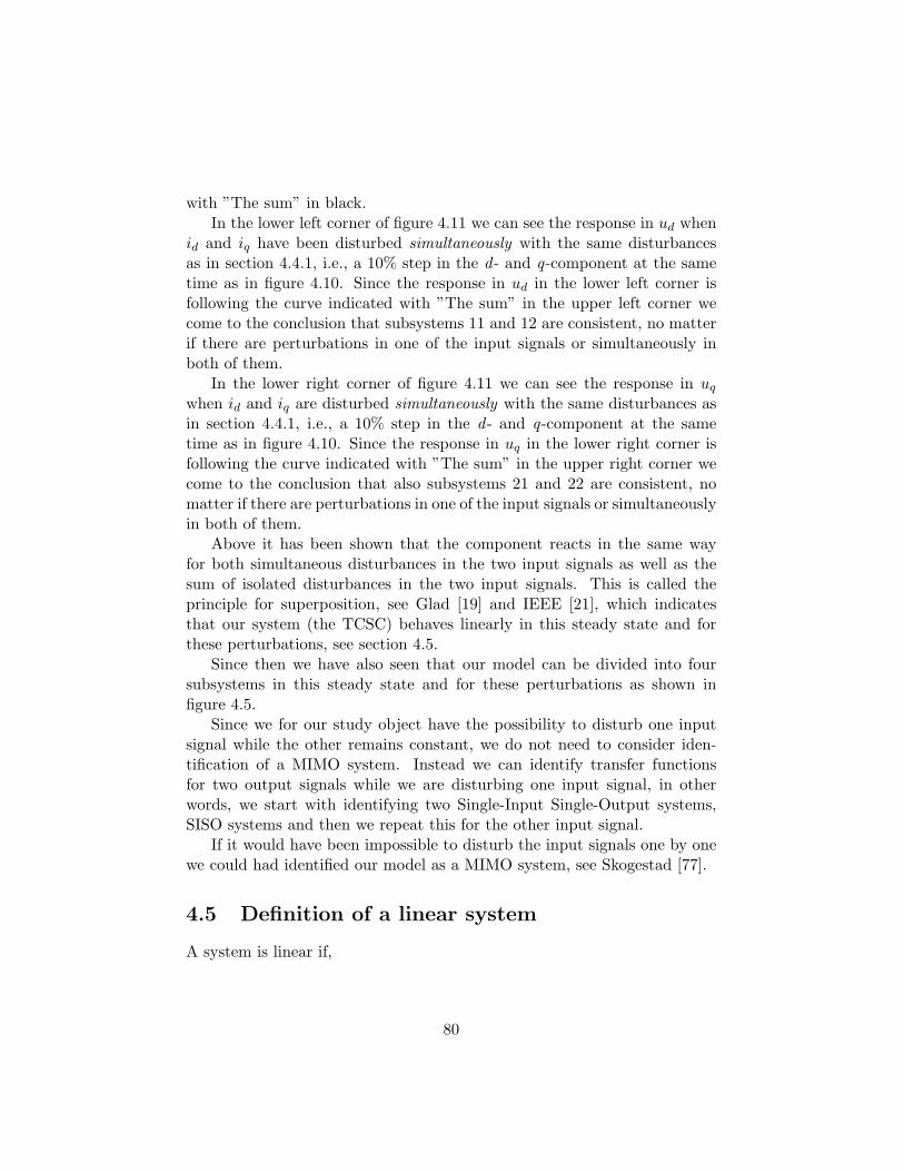
with ”The sum” in black.In the lower left corner of figure 4.11 we can see the response in ud when

id and iq have been disturbed simultaneously with the same disturbancesas in section 4.4.1, i.e., a 10% step in the d - and q-component at the sametime as in figure 4.10. Since the response in ud in the lower left corner isfollowing the curve indicated with ”The sum” in the upper left corner wecome to the conclusion that subsystems 11 and 12 are consistent, no matterif there are perturbations in one of the input signals or simultaneously inboth of them.

In the lower right corner of figure 4.11 we can see the response in uq

when id and iq are disturbed simultaneously with the same disturbances asin section 4.4.1, i.e., a 10% step in the d - and q-component at the sametime as in figure 4.10. Since the response in uq in the lower right corner isfollowing the curve indicated with ”The sum” in the upper right corner wecome to the conclusion that also subsystems 21 and 22 are consistent, nomatter if there are perturbations in one of the input signals or simultaneouslyin both of them.

Above it has been shown that the component reacts in the same wayfor both simultaneous disturbances in the two input signals as well as thesum of isolated disturbances in the two input signals. This is called theprinciple for superposition, see Glad [19] and IEEE [21], which indicatesthat our system (the TCSC) behaves linearly in this steady state and forthese perturbations, see section 4.5.

Since then we have also seen that our model can be divided into foursubsystems in this steady state and for these perturbations as shown infigure 4.5.

Since we for our study object have the possibility to disturb one inputsignal while the other remains constant, we do not need to consider iden-tification of a MIMO system. Instead we can identify transfer functionsfor two output signals while we are disturbing one input signal, in otherwords, we start with identifying two Single-Input Single-Output systems,SISO systems and then we repeat this for the other input signal.

If it would have been impossible to disturb the input signals one by onewe could had identified our model as a MIMO system, see Skogestad [77].

4.5 Definition of a linear system

A system is linear if,

80

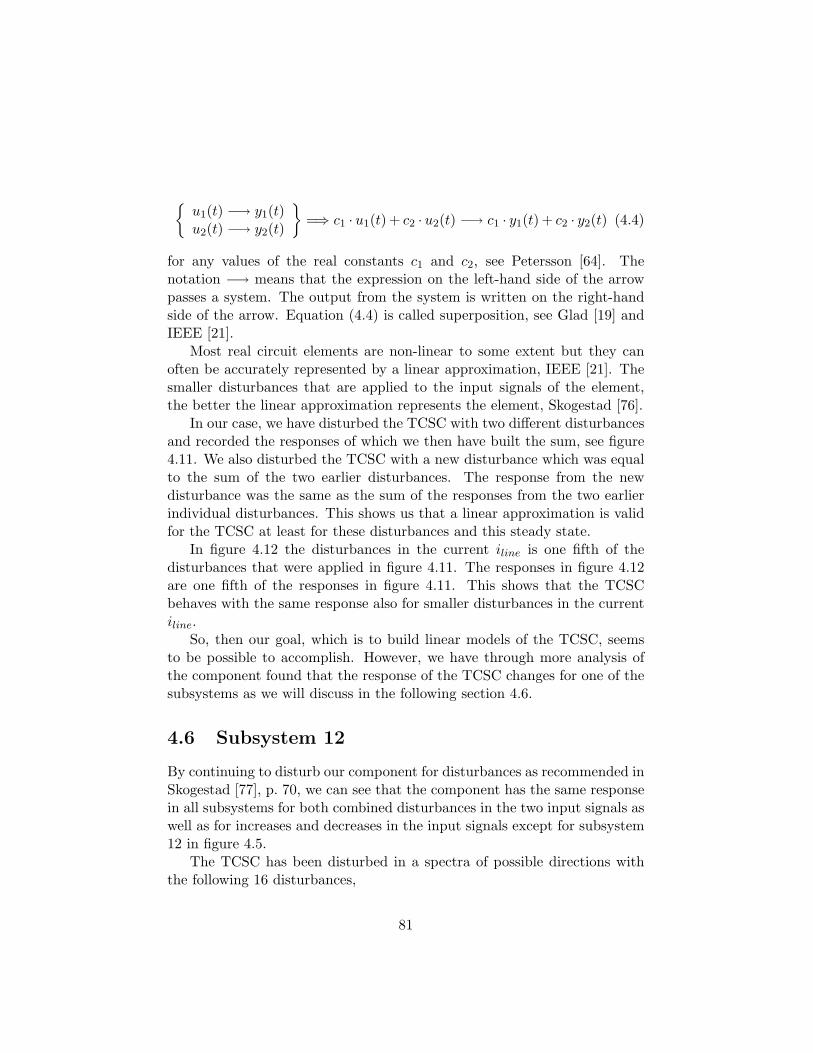
u1(t) −→ y1(t)u2(t) −→ y2(t)

=⇒ c1 · u1(t) + c2 · u2(t) −→ c1 · y1(t) + c2 · y2(t) (4.4)

for any values of the real constants c1 and c2, see Petersson [64]. Thenotation −→ means that the expression on the left-hand side of the arrowpasses a system. The output from the system is written on the right-handside of the arrow. Equation (4.4) is called superposition, see Glad [19] andIEEE [21].

Most real circuit elements are non-linear to some extent but they canoften be accurately represented by a linear approximation, IEEE [21]. Thesmaller disturbances that are applied to the input signals of the element,the better the linear approximation represents the element, Skogestad [76].

In our case, we have disturbed the TCSC with two different disturbancesand recorded the responses of which we then have built the sum, see figure4.11. We also disturbed the TCSC with a new disturbance which was equalto the sum of the two earlier disturbances. The response from the newdisturbance was the same as the sum of the responses from the two earlierindividual disturbances. This shows us that a linear approximation is validfor the TCSC at least for these disturbances and this steady state.

In figure 4.12 the disturbances in the current iline is one fifth of thedisturbances that were applied in figure 4.11. The responses in figure 4.12are one fifth of the responses in figure 4.11. This shows that the TCSCbehaves with the same response also for smaller disturbances in the currentiline.

So, then our goal, which is to build linear models of the TCSC, seemsto be possible to accomplish. However, we have through more analysis ofthe component found that the response of the TCSC changes for one of thesubsystems as we will discuss in the following section 4.6.

4.6 Subsystem 12

By continuing to disturb our component for disturbances as recommended inSkogestad [77], p. 70, we can see that the component has the same responsein all subsystems for both combined disturbances in the two input signals aswell as for increases and decreases in the input signals except for subsystem12 in figure 4.5.

The TCSC has been disturbed in a spectra of possible directions withthe following 16 disturbances,

81

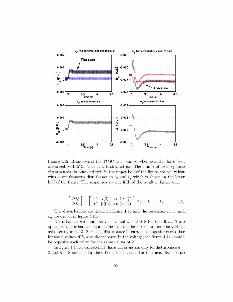
3 3.5 4 4.5-0.001

0

0.001

0.002

Time (s)

u d (p.u

.)

ud, two perturbations and the sum

3 3.5 4 4.5-0.028

-0.027

-0.026

-0.025

Time (s)

u q (p.u

.)

uq, two perturbations and the sum

3 3.5 4 4.5-0.001

0

0.001

0.002

Time (s)

u d (p.u

.)

ud, one perturbation

3 3.5 4 4.5-0.028

-0.027

-0.026

-0.025

Time (s)

u q (p.u

.)

uq, one perturbation

The sum

The sum

Figure 4.12: Responses of the TCSC in ud and uq when id and iq have beendisturbed with 2%. The sum (indicated as ”The sum”) of two separatedisturbances (in blue and red) in the upper half of the figure are equivalentwith a simultaneous disturbance in id and iq which is shown in the lowerhalf of the figure. The responses are one fifth of the result in figure 4.11.

[∆id∆iq

]=

[0.1 · |i(0)| · cos (n · π

8 )0.1 · |i(0)| · sin (n · π

8 )

]∨ n = 0, . . . , 15. (4.5)

The disturbances are drawn in figure 4.13 and the responses in ud anduq are drawn in figure 4.14.

Disturbances with number n = k and n = k + 8 for k = 0, . . . , 7 areopposite each other, i.e., symmetric in both the horizontal and the verticalaxis, see figure 4.13. Since the disturbance in current is opposite each otherfor these values of k, also the response in the voltage, see figure 4.14, shouldbe opposite each other for the same values of k.

In figure 4.14 we can see that this is the situation only for disturbance n =0 and n = 8 and not for the other disturbances. For instance, disturbance

82

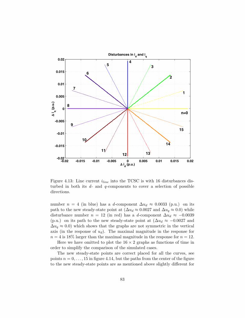
-0.02 -0.015 -0.01 -0.005 0 0.005 0.01 0.015 0.02-0.02

-0.015

-0.01

-0.005

0

0.005

0.01

0.015

0.02

∆∆∆∆ id (p.u.)

∆∆ ∆∆ i q (p

.u.)

Disturbances in id and i

q

n=0

1

2

3 4

5

6

7

8

9

10

11 12 13

14

15

Figure 4.13: Line current iline into the TCSC is with 16 disturbances dis-turbed in both its d - and q-components to cover a selection of possibledirections.

number n = 4 (in blue) has a d -component ∆ud ≈ 0.0033 (p.u.) on itspath to the new steady-state point at (∆ud ≈ 0.0027 and ∆uq ≈ 0.0) whiledisturbance number n = 12 (in red) has a d -component ∆ud ≈ −0.0039(p.u.) on its path to the new steady-state point at (∆ud ≈ −0.0027 and∆uq ≈ 0.0) which shows that the graphs are not symmetric in the verticalaxis (in the response of ud). The maximal magnitude in the response forn = 4 is 18% larger than the maximal magnitude in the response for n = 12.

Here we have omitted to plot the 16 × 2 graphs as functions of time inorder to simplify the comparison of the simulated cases.

The new steady-state points are correct placed for all the curves, seepoints n = 0, . . . , 15 in figure 4.14, but the paths from the center of the figureto the new steady-state points are as mentioned above slightly different for

83

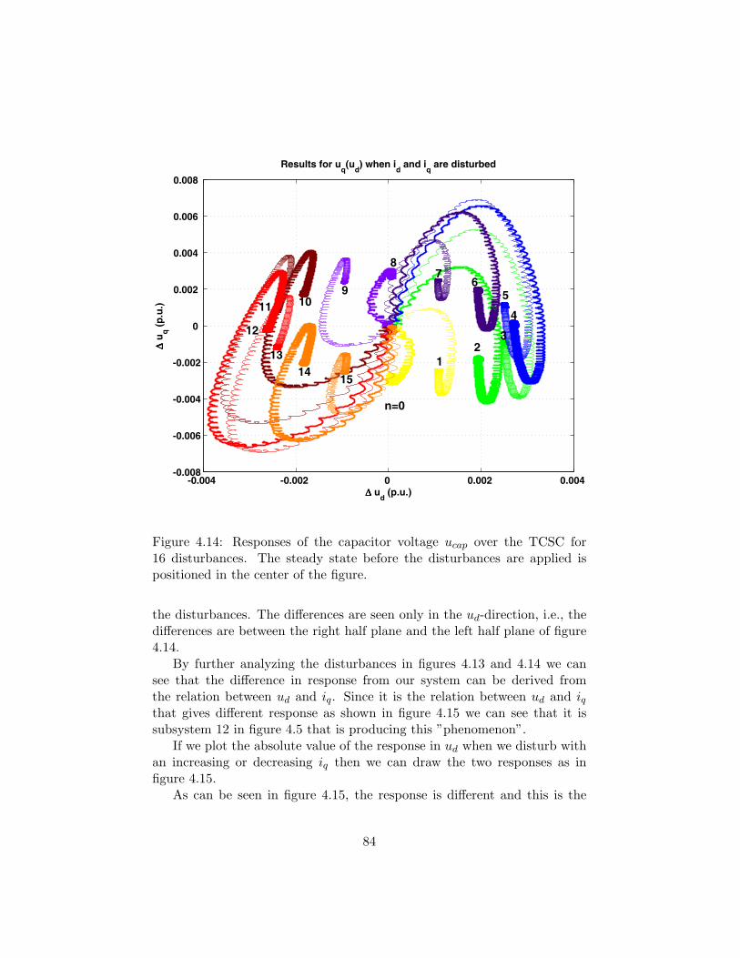
-0.004 -0.002 0 0.002 0.004 -0.008

-0.006

-0.004

-0.002

0

0.002

0.004

0.006

0.008

∆∆∆∆ ud (p.u.)

∆∆ ∆∆ u q (p

.u.)

Results for uq(u

d) when i

d and i

q are disturbed

n=0

1 2

3

4

5 6

7 8

9 10 11

12

13 14 15

Figure 4.14: Responses of the capacitor voltage ucap over the TCSC for16 disturbances. The steady state before the disturbances are applied ispositioned in the center of the figure.

the disturbances. The differences are seen only in the ud-direction, i.e., thedifferences are between the right half plane and the left half plane of figure4.14.

By further analyzing the disturbances in figures 4.13 and 4.14 we cansee that the difference in response from our system can be derived fromthe relation between ud and iq. Since it is the relation between ud and iqthat gives different response as shown in figure 4.15 we can see that it issubsystem 12 in figure 4.5 that is producing this ”phenomenon”.

If we plot the absolute value of the response in ud when we disturb withan increasing or decreasing iq then we can draw the two responses as infigure 4.15.

As can be seen in figure 4.15, the response is different and this is the

84

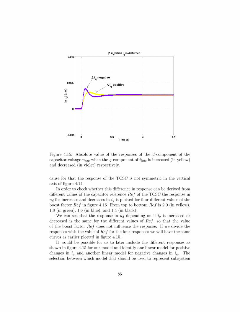
3 3.5 4 4.5-0.005

0

0.005

0.010

Time (s)

| ∆∆ ∆∆ u

d| (p.

u.)

|∆∆∆∆ ud| when i

q is disturbed

∆∆∆∆ iq positive

∆∆∆∆ iq negative

Figure 4.15: Absolute value of the responses of the d -component of thecapacitor voltage ucap when the q-component of iline is increased (in yellow)and decreased (in violet) respectively.

cause for that the response of the TCSC is not symmetric in the verticalaxis of figure 4.14.

In order to check whether this difference in response can be derived fromdifferent values of the capacitor reference Ref of the TCSC the response inud for increases and decreases in iq is plotted for four different values of theboost factor Ref in figure 4.16. From top to bottom Ref is 2.0 (in yellow),1.8 (in green), 1.6 (in blue), and 1.4 (in black).

We can see that the response in ud depending on if iq is increased ordecreased is the same for the different values of Ref , so that the valueof the boost factor Ref does not influence the response. If we divide theresponses with the value of Ref for the four responses we will have the samecurves as earlier plotted in figure 4.15.

It would be possible for us to later include the different responses asshown in figure 4.15 for our model and identify one linear model for positivechanges in iq and another linear model for negative changes in iq. Theselection between which model that should be used to represent subsystem

85

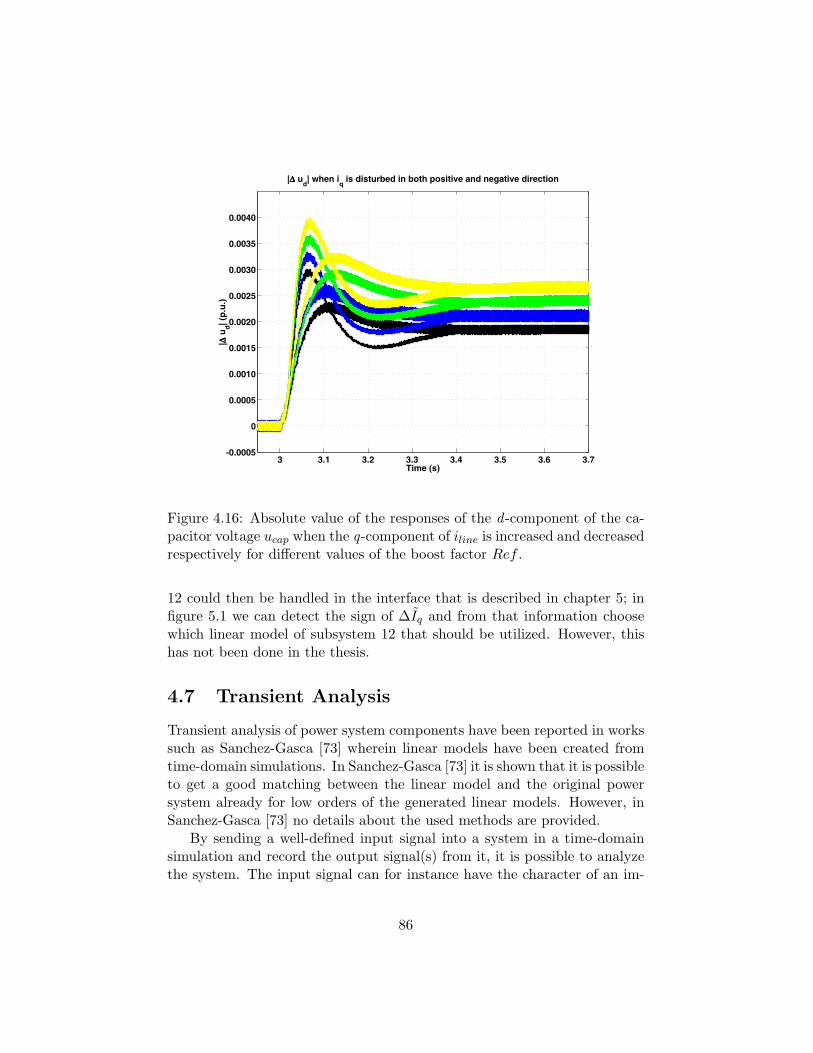
3 3.1 3.2 3.3 3.4 3.5 3.6 3.7-0.0005

0

0.0005

0.0010

0.0015

0.0020

0.0025

0.0030

0.0035

0.0040

Time (s)

| ∆∆ ∆∆ u

d| (p.

u.)

|∆∆∆∆ ud| when i

q is disturbed in both positive and negative direction

Figure 4.16: Absolute value of the responses of the d -component of the ca-pacitor voltage ucap when the q-component of iline is increased and decreasedrespectively for different values of the boost factor Ref .

12 could then be handled in the interface that is described in chapter 5; infigure 5.1 we can detect the sign of ∆Iq and from that information choosewhich linear model of subsystem 12 that should be utilized. However, thishas not been done in the thesis.

4.7 Transient Analysis

Transient analysis of power system components have been reported in workssuch as Sanchez-Gasca [73] wherein linear models have been created fromtime-domain simulations. In Sanchez-Gasca [73] it is shown that it is possibleto get a good matching between the linear model and the original powersystem already for low orders of the generated linear models. However, inSanchez-Gasca [73] no details about the used methods are provided.

By sending a well-defined input signal into a system in a time-domainsimulation and record the output signal(s) from it, it is possible to analyzethe system. The input signal can for instance have the character of an im-

86

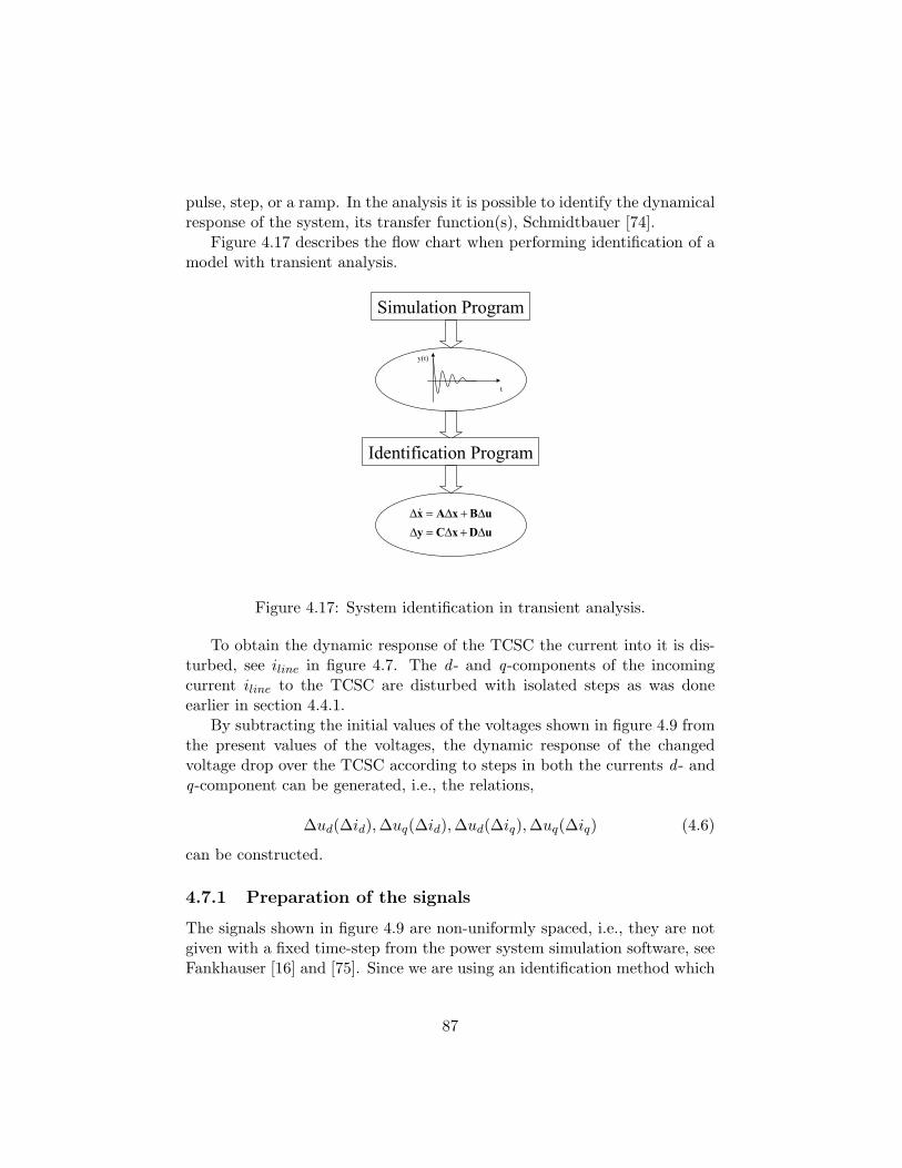
pulse, step, or a ramp. In the analysis it is possible to identify the dynamicalresponse of the system, its transfer function(s), Schmidtbauer [74].

Figure 4.17 describes the flow chart when performing identification of amodel with transient analysis.

Simulation Program

t

y(t)

uBxAx ∆+∆=∆&

∆ ∆ ∆y C x D u= +

Identification Program

Figure 4.17: System identification in transient analysis.

To obtain the dynamic response of the TCSC the current into it is dis-turbed, see iline in figure 4.7. The d - and q-components of the incomingcurrent iline to the TCSC are disturbed with isolated steps as was doneearlier in section 4.4.1.

By subtracting the initial values of the voltages shown in figure 4.9 fromthe present values of the voltages, the dynamic response of the changedvoltage drop over the TCSC according to steps in both the currents d - andq-component can be generated, i.e., the relations,

∆ud(∆id),∆uq(∆id),∆ud(∆iq),∆uq(∆iq) (4.6)

can be constructed.

4.7.1 Preparation of the signals

The signals shown in figure 4.9 are non-uniformly spaced, i.e., they are notgiven with a fixed time-step from the power system simulation software, seeFankhauser [16] and [75]. Since we are using an identification method which

87

demands equidistant sampled signals, see Ljung [41], we have to make thesignals equidistant sampled. So, first the four voltage signals in figure 4.9are sampled with uniformly spaced sampling. By studying the signals itcan be observed that they, after have been filtered with the filter mentionedin section 3.4, still contain harmonics, but the harmonics have been signifi-cantly reduced. Frequencies higher than the sixth harmonic (360 (Hz)) havesignificantly been removed from the signals. The sampling frequency is setto fs = 10 (kHz) to be sure of that no frequencies are folded into the fre-quency spectrum of interest. With sampling frequency fs = 10 (kHz), theNyquist frequency is 5 (kHz) according to the sampling theorem, i.e., fre-quencies above 5 (kHz) could be folded - aliased into the desired frequencyspectrum, see Proakis [65]. This is however not the situation since we havesignificantly reduced frequencies higher than 360 (Hz) in the signals withthe earlier introduced filter.

Figure 4.18 shows a detailed flow chart of the identification process intransient analysis.

Before continuing, the signals are again filtered with a first-order filter,this time with the time constant T = 0.005 (s), to decrease the magnitude ofthe sixth harmonic. Afterwards the signals are re-sampled with the samplingfrequency fs = 500 (Hz) so that the signals are given with the time step 0.002(s). Re-sampling has here been made with the Nyquist frequency 250 (Hz)and the small amount of the sixth harmonic 360 (Hz) that still exists in thesignals may have been folded into the frequency spectrum and appears as140 (Hz). However, this has been checked in the re-sampled signals and isnot causing any problem in the identification process, see section 4.7.2.

The last re-sampling is made since the number of samples is unnecessarylarge to describe the slow dynamics of the signals and it has been found thatit is easier to identify difference equations for the transfer functions as inequation (4.7) when the signals are given with a larger time step.

4.7.2 Identification of the four subsystems

By using Matlab’s System Identification Toolbox, Ljung [40, 41] to buildARX-models for the four relations, transfer functions have been found. Themethod works in the time-discrete domain. The input to the method isuniformly spaced sampled values of input and output signals of an unknownsystem. The following difference equation is then identified,

y(t)+e1y(t−1)+. . .+eney(t−ne) = f1u(t−1)+. . .+fnfu(t−nf )+v(t). (4.7)

88

*

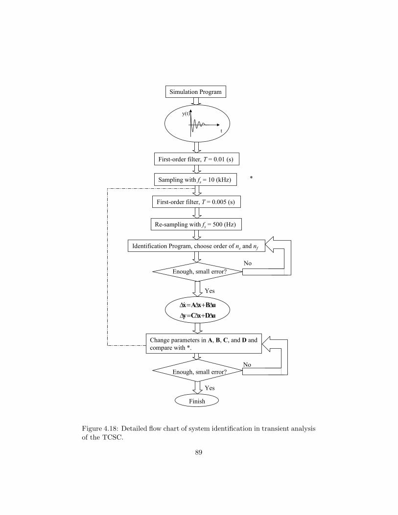
Simulation Program

Finish

t

y(t)

uBxAx ∆+∆=∆&

uDxCy ∆+∆=∆

First-order filter, T = 0.01 (s)

Sampling with fs = 10 (kHz)

Re-sampling with fs = 500 (Hz)

No

Yes

Enough, small error?

No

Yes

Enough, small error?

Identification Program, choose order of ne and nf

First-order filter, T = 0.005 (s)

Change parameters in A, B, C, and D andcompare with *.

Figure 4.18: Detailed flow chart of system identification in transient analysisof the TCSC.

89

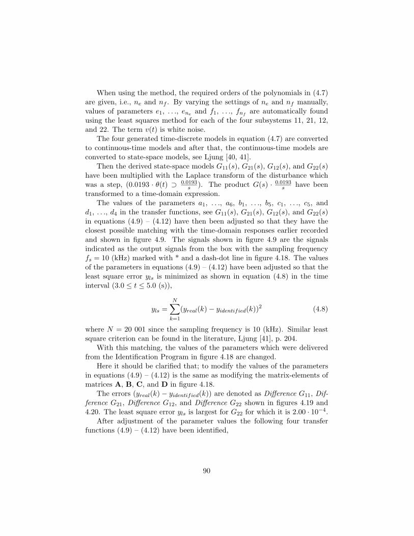
When using the method, the required orders of the polynomials in (4.7)are given, i.e., ne and nf . By varying the settings of ne and nf manually,values of parameters e1, . . ., ene and f1, . . ., fnf

are automatically foundusing the least squares method for each of the four subsystems 11, 21, 12,and 22. The term v(t) is white noise.

The four generated time-discrete models in equation (4.7) are convertedto continuous-time models and after that, the continuous-time models areconverted to state-space models, see Ljung [40, 41].

Then the derived state-space models G11(s), G21(s), G12(s), and G22(s)have been multiplied with the Laplace transform of the disturbance whichwas a step, (0.0193 · θ(t) ⊃ 0.0193

s ). The product G(s) · 0.0193s have been

transformed to a time-domain expression.The values of the parameters a1, . . ., a6, b1, . . ., b5, c1, . . ., c5, and

d1, . . ., d4 in the transfer functions, see G11(s), G21(s), G12(s), and G22(s)in equations (4.9) – (4.12) have then been adjusted so that they have theclosest possible matching with the time-domain responses earlier recordedand shown in figure 4.9. The signals shown in figure 4.9 are the signalsindicated as the output signals from the box with the sampling frequencyfs = 10 (kHz) marked with * and a dash-dot line in figure 4.18. The valuesof the parameters in equations (4.9) – (4.12) have been adjusted so that theleast square error yls is minimized as shown in equation (4.8) in the timeinterval (3.0 ≤ t ≤ 5.0 (s)),

yls =N∑

k=1

(yreal(k)− yidentified(k))2 (4.8)

where N = 20 001 since the sampling frequency is 10 (kHz). Similar leastsquare criterion can be found in the literature, Ljung [41], p. 204.

With this matching, the values of the parameters which were deliveredfrom the Identification Program in figure 4.18 are changed.

Here it should be clarified that; to modify the values of the parametersin equations (4.9) – (4.12) is the same as modifying the matrix-elements ofmatrices A, B, C, and D in figure 4.18.

The errors (yreal(k)− yidentified(k)) are denoted as Difference G11, Dif-ference G21, Difference G12, and Difference G22 shown in figures 4.19 and4.20. The least square error yls is largest for G22 for which it is 2.00 · 10−4.

After adjustment of the parameter values the following four transferfunctions (4.9) – (4.12) have been identified,

90

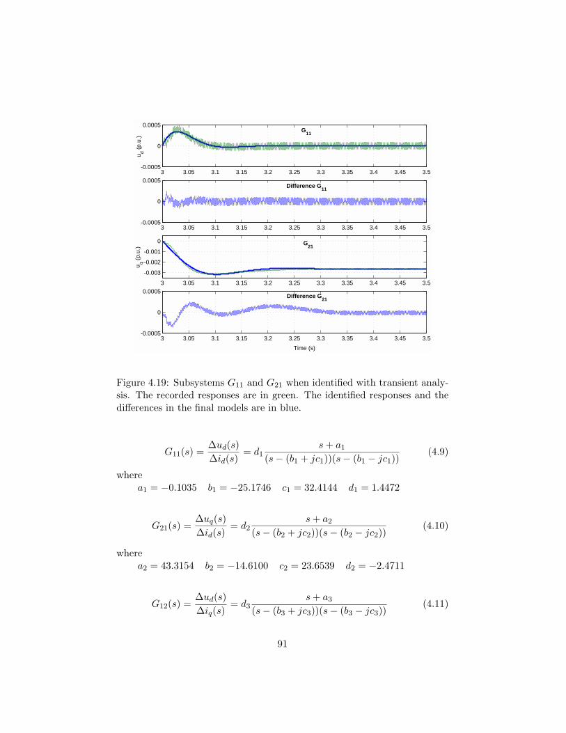
3 3.05 3.1 3.15 3.2 3.25 3.3 3.35 3.4 3.45 3.5-0.0005

0

0.0005G11

u d (p.u

.)

3 3.05 3.1 3.15 3.2 3.25 3.3 3.35 3.4 3.45 3.5-0.0005

0

0.0005Difference G11

3 3.05 3.1 3.15 3.2 3.25 3.3 3.35 3.4 3.45 3.5

-0.003

-0.002

-0.001

0 G21

u q (p.u

.)

3 3.05 3.1 3.15 3.2 3.25 3.3 3.35 3.4 3.45 3.5-0.0005

0

0.0005Difference G21

Time (s)

Figure 4.19: Subsystems G11 and G21 when identified with transient analy-sis. The recorded responses are in green. The identified responses and thedifferences in the final models are in blue.

G11(s) =∆ud(s)∆id(s)

= d1s + a1

(s− (b1 + jc1))(s− (b1 − jc1))(4.9)

wherea1 = −0.1035 b1 = −25.1746 c1 = 32.4144 d1 = 1.4472

G21(s) =∆uq(s)∆id(s)

= d2s + a2

(s− (b2 + jc2))(s− (b2 − jc2))(4.10)

wherea2 = 43.3154 b2 = −14.6100 c2 = 23.6539 d2 = −2.4711

G12(s) =∆ud(s)∆iq(s)

= d3s + a3

(s− (b3 + jc3))(s− (b3 − jc3))(4.11)

91

3 3.05 3.1 3.15 3.2 3.25 3.3 3.35 3.4 3.45 3.5

0

0.001

0.002

0.003

G12u d (p

.u.)

3 3.05 3.1 3.15 3.2 3.25 3.3 3.35 3.4 3.45 3.5-0.0005

0

0.0005Difference G12

3 3.05 3.1 3.15 3.2 3.25 3.3 3.35 3.4 3.45 3.5-0.004

0

0.004

0.008G22

u q (p.u

.)

3 3.05 3.1 3.15 3.2 3.25 3.3 3.35 3.4 3.45 3.5-0.0005

0

0.0005 Difference G22

Time (s)

Figure 4.20: Subsystems G12 and G22 when identified with transient analy-sis. The recorded responses are in green. The identified responses and thedifferences in the final models are in blue.

wherea3 = 14.9983 b3 = −10.8263 c3 = 13.6453 d3 = 2.7826

G22(s) =∆uq(s)∆iq(s)

= d4(s + a4)

(s− (b4 + jc4))(s− (b4 − jc4))·

· (s + a5)(s + a6)(s− (b5 + jc5))(s− (b5 − jc5))

(4.12)

wherea4 = 0.7634 b4 = −26.6035 c4 = 32.8667 d4 = 9.7379a5 = 107.4998 b5 = −8.1031 c5 = 8.4132a6 = −0.7740

In equations (4.9) – (4.12) all poles (roots of the denominator) are in theleft half plane.

In equations (4.9) and (4.12) there are two right half plane zeros (rootsof the numerator) at 0.1035 and 0.7740 (1/s) respectively. If the aim had

92

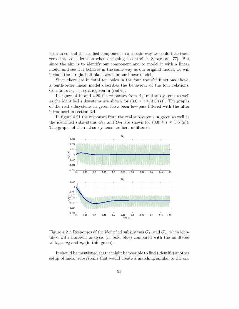
been to control the studied component in a certain way we could take thesezeros into consideration when designing a controller, Skogestad [77]. Butsince the aim is to identify our component and to model it with a linearmodel and see if it behaves in the same way as our original model, we willinclude these right half plane zeros in our linear model.

Since there are in total ten poles in the four transfer functions above,a tenth-order linear model describes the behaviour of the four relations.Constants c1, . . ., c5 are given in (rad/s).

In figures 4.19 and 4.20 the responses from the real subsystems as wellas the identified subsystems are shown for (3.0 ≤ t ≤ 3.5 (s)). The graphsof the real subsystems in green have been low-pass filtered with the filterintroduced in section 3.4.

In figure 4.21 the responses from the real subsystems in green as well asthe identified subsystems G11 and G21 are shown for (3.0 ≤ t ≤ 3.5 (s)).The graphs of the real subsystems are here unfiltered.

3 3.05 3.1 3.15 3.2 3.25 3.3 3.35 3.4 3.45 3.5-0.003

-0.002

-0.001

0

0.001

0.002

0.003G

11

u d (p.u

.)

3 3.05 3.1 3.15 3.2 3.25 3.3 3.35 3.4 3.45 3.5-0.005

-0.004

-0.003

-0.002

-0.001

0

0.001G

21

u q (p.u

.)

Time (s)

Figure 4.21: Responses of the identified subsystems G11 and G21 when iden-tified with transient analysis (in bold blue) compared with the unfilteredvoltages ud and uq (in thin green).

It should be mentioned that it might be possible to find (identify) anothersetup of linear subsystems that would create a matching similar to the one

93

shown in figures 4.19 and 4.20. However, we have here seen that the leastsquare errors are acceptably small for the identified linear model. Thereforewe continue in chapters 6 and 7 to investigate whether it represent thedynamics of the TCSC.

4.7.3 A check of the linear model developed from transientanalysis

Before continuing we plot the frequency response of the developed modelwith transient analysis here in section 4.7. The results are shown in figure4.22.

When comparing figure 4.22 with the figures 4.27 and 4.28 (that will becreated in the next section) we can see that the frequency responses are verysimilar for the two linear models.

4.8 Frequency Analysis

By sending a sinus-formed input signal into a system in a time-domainsimulation and record the output signal(s), and repeat this for a numberof frequencies and create a frequency spectra, it is possible to analyze thesystem. In the analysis it is possible to identify the dynamical response ofthe system, its transfer function(s), see Schmidtbauer [74].

Figure 4.23 describes the flow chart when performing identification of amodel with frequency analysis.

If the input signal of a linear system is excited (perturbed) by a periodicsignal composed of specific harmonic(s) then the output signal will also beperiodic and contain the same harmonic(s). Unlike linear systems, outputsignals from non-linear system may contain harmonics that do not appearin the input sequence, see Docter [12]. Since it is not possible for a linearmodel to produce such harmonics, these harmonics are impossible to modelwith linear techniques and should be removed from the data. This is easilyaccomplished by decomposing the output data with the Fast Fourier Trans-form (FFT) into two parts; the harmonic(s) that are in the input sequence,and those that are not.

The linearity of the TCSC has been investigated in sections 4.4 – 4.6 sotherefore it should be conceivable to apply frequency analysis to our studyobject.

To obtain the dynamic response of the TCSC, the current into it, seeiline in figure 4.7, is disturbed. The d - and q-components of the incoming

94

1 10 100

-60

-40

-20

0

Mag

nitu

de, u

d/i d (dB

)

1 10 100-200

-100

0

100

200

Pha

se, u

d/i d (deg

rees

)

Angular speed (rad/s)

1 10 100

-60

-40

-20

0

Mag

nitu

de, u

q/i d (dB

)

1 10 100-200

-100

0

100

200

Pha

se, u

q/i d (deg

rees

)

Angular speed (rad/s)

1 10 100

-60

-40

-20

0

Mag

nitu

de, u

d/i q (dB

)

1 10 100

-300

-200

-100

0

Pha

se, u

d/i q (deg

rees

)

Angular speed (rad/s)

1 10 100

-60

-40

-20

0

Mag

nitu

de, u

q/i q (dB

)

1 10 100

0

100

200

300

Pha

se, u

q/i q (deg

rees

)

Angular speed (rad/s)

Figure 4.22: Frequency response of the linear model identified with transientanalysis.

95

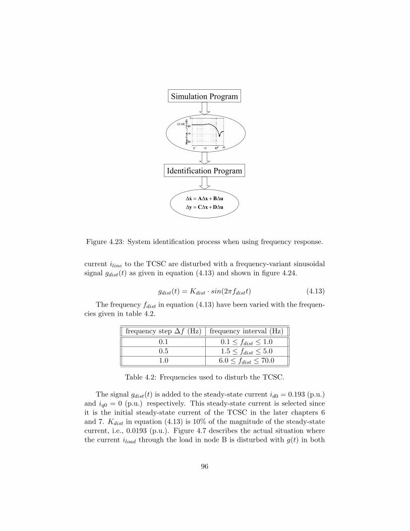
Simulation Program

uBxAx ∆+∆=∆&

∆ ∆ ∆y C x D u= +

Identification Program

ω

|y(ω)|

Figure 4.23: System identification process when using frequency response.

current iline to the TCSC are disturbed with a frequency-variant sinusoidalsignal gdist(t) as given in equation (4.13) and shown in figure 4.24.

gdist(t) = Kdist · sin(2πfdistt) (4.13)

The frequency fdist in equation (4.13) have been varied with the frequen-cies given in table 4.2.

frequency step ∆f (Hz) frequency interval (Hz)0.1 0.1 ≤ fdist ≤ 1.00.5 1.5 ≤ fdist ≤ 5.01.0 6.0 ≤ fdist ≤ 70.0

Table 4.2: Frequencies used to disturb the TCSC.

The signal gdist(t) is added to the steady-state current id0 = 0.193 (p.u.)and iq0 = 0 (p.u.) respectively. This steady-state current is selected sinceit is the initial steady-state current of the TCSC in the later chapters 6and 7. Kdist in equation (4.13) is 10% of the magnitude of the steady-statecurrent, i.e., 0.0193 (p.u.). Figure 4.7 describes the actual situation wherethe current iload through the load in node B is disturbed with g(t) in both

96

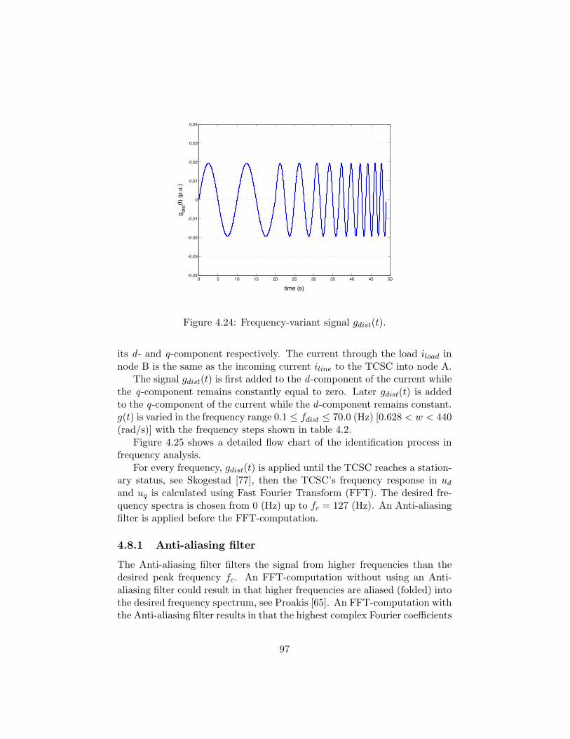
0 5 10 15 20 25 30 35 40 45 50-0.04

-0.03

-0.02

-0.01

0

0.01

0.02

0.03

0.04

g dist

(t) (p

.u.)

time (s)

Figure 4.24: Frequency-variant signal gdist(t).

its d - and q-component respectively. The current through the load iload innode B is the same as the incoming current iline to the TCSC into node A.

The signal gdist(t) is first added to the d -component of the current whilethe q-component remains constantly equal to zero. Later gdist(t) is addedto the q-component of the current while the d -component remains constant.g(t) is varied in the frequency range 0.1 ≤ fdist ≤ 70.0 (Hz) [0.628 < w < 440(rad/s)] with the frequency steps shown in table 4.2.

Figure 4.25 shows a detailed flow chart of the identification process infrequency analysis.

For every frequency, gdist(t) is applied until the TCSC reaches a station-ary status, see Skogestad [77], then the TCSC’s frequency response in ud

and uq is calculated using Fast Fourier Transform (FFT). The desired fre-quency spectra is chosen from 0 (Hz) up to fc = 127 (Hz). An Anti-aliasingfilter is applied before the FFT-computation.

4.8.1 Anti-aliasing filter

The Anti-aliasing filter filters the signal from higher frequencies than thedesired peak frequency fc. An FFT-computation without using an Anti-aliasing filter could result in that higher frequencies are aliased (folded) intothe desired frequency spectrum, see Proakis [65]. An FFT-computation withthe Anti-aliasing filter results in that the highest complex Fourier coefficients

97

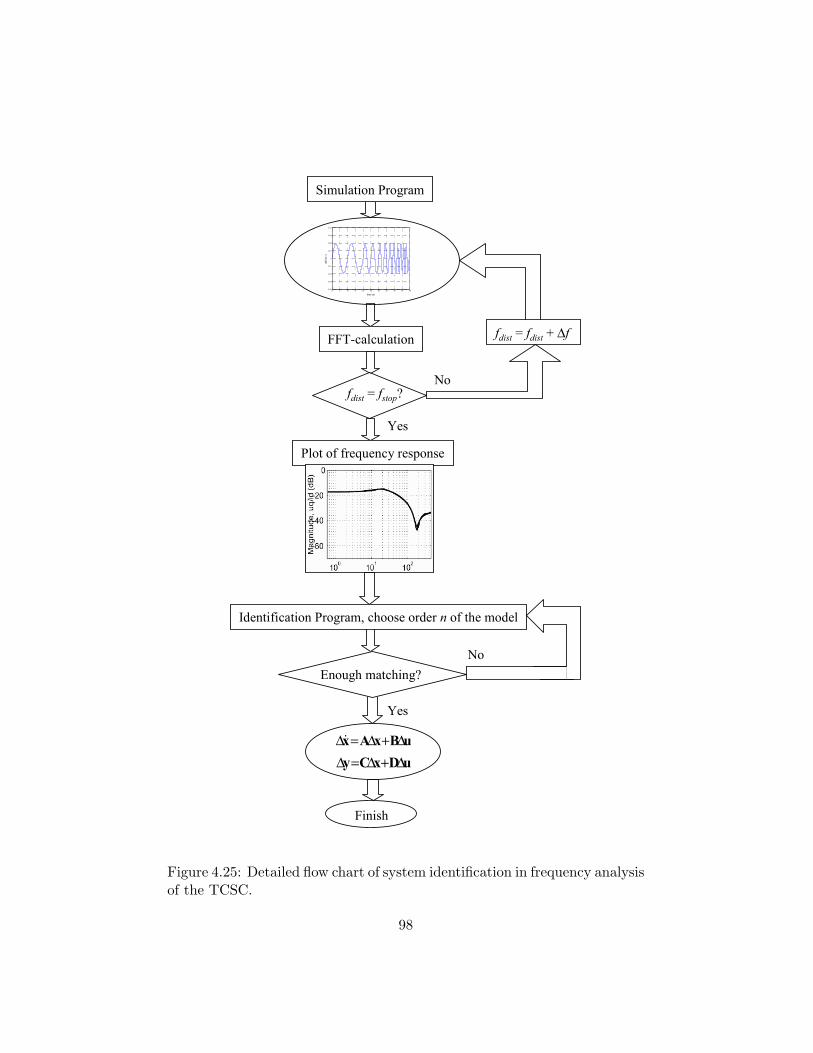
0 5 10 15 20 25 30 35 40 45 50-0.04

-0.03

-0.02

-0.01

0

0.01

0.02

0.03

0.04

g(t)

(p.

u.)

time (s)

Simulation Program

Finish

FFT-calculation

No

Yes

Enough matching?

Identification Program, choose order n of the model

Plot of frequency response

No

Yes

fdist = fstop?

fdist = fdist + ∆f

uBxAx ∆+∆=∆&

uDxCy ∆+∆=∆

Figure 4.25: Detailed flow chart of system identification in frequency analysisof the TCSC.

98

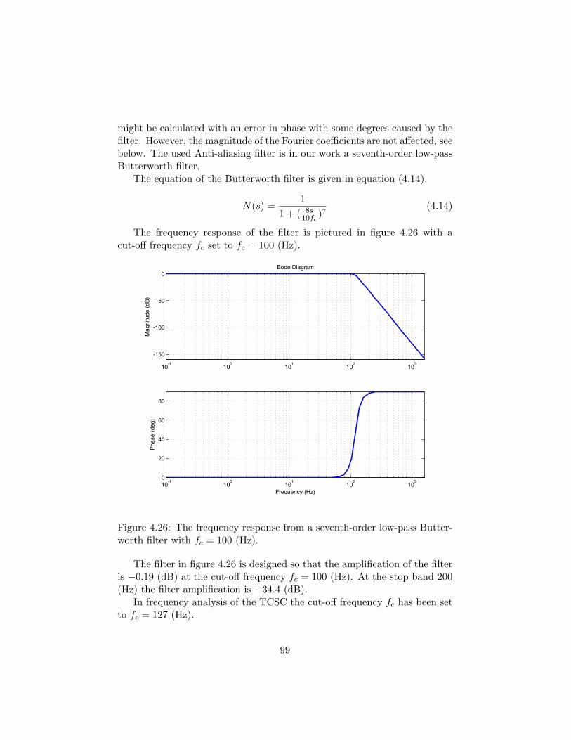
might be calculated with an error in phase with some degrees caused by thefilter. However, the magnitude of the Fourier coefficients are not affected, seebelow. The used Anti-aliasing filter is in our work a seventh-order low-passButterworth filter.

The equation of the Butterworth filter is given in equation (4.14).

N(s) =1

1 + ( 8s10fc

)7(4.14)

The frequency response of the filter is pictured in figure 4.26 with acut-off frequency fc set to fc = 100 (Hz).

10-1

100

101

102

103

-150

-100

-50

0Bode Diagram

Mag

nitu

de (d

B)

10-1

100

101

102

103

0

20

40

60

80

Pha

se (d

eg)

Frequency (Hz)

Figure 4.26: The frequency response from a seventh-order low-pass Butter-worth filter with fc = 100 (Hz).

The filter in figure 4.26 is designed so that the amplification of the filteris −0.19 (dB) at the cut-off frequency fc = 100 (Hz). At the stop band 200(Hz) the filter amplification is −34.4 (dB).

In frequency analysis of the TCSC the cut-off frequency fc has been setto fc = 127 (Hz).

99

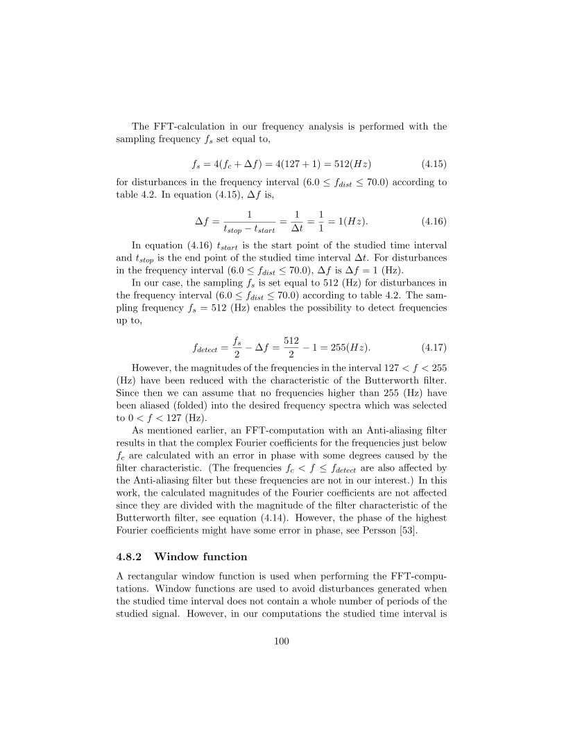
The FFT-calculation in our frequency analysis is performed with thesampling frequency fs set equal to,

fs = 4(fc + ∆f) = 4(127 + 1) = 512(Hz) (4.15)

for disturbances in the frequency interval (6.0 ≤ fdist ≤ 70.0) according totable 4.2. In equation (4.15), ∆f is,

∆f =1

tstop − tstart=

1∆t

=11

= 1(Hz). (4.16)

In equation (4.16) tstart is the start point of the studied time intervaland tstop is the end point of the studied time interval ∆t. For disturbancesin the frequency interval (6.0 ≤ fdist ≤ 70.0), ∆f is ∆f = 1 (Hz).

In our case, the sampling fs is set equal to 512 (Hz) for disturbances inthe frequency interval (6.0 ≤ fdist ≤ 70.0) according to table 4.2. The sam-pling frequency fs = 512 (Hz) enables the possibility to detect frequenciesup to,

fdetect =fs

2−∆f =

5122− 1 = 255(Hz). (4.17)

However, the magnitudes of the frequencies in the interval 127 < f < 255(Hz) have been reduced with the characteristic of the Butterworth filter.Since then we can assume that no frequencies higher than 255 (Hz) havebeen aliased (folded) into the desired frequency spectra which was selectedto 0 < f < 127 (Hz).

As mentioned earlier, an FFT-computation with an Anti-aliasing filterresults in that the complex Fourier coefficients for the frequencies just belowfc are calculated with an error in phase with some degrees caused by thefilter characteristic. (The frequencies fc < f ≤ fdetect are also affected bythe Anti-aliasing filter but these frequencies are not in our interest.) In thiswork, the calculated magnitudes of the Fourier coefficients are not affectedsince they are divided with the magnitude of the filter characteristic of theButterworth filter, see equation (4.14). However, the phase of the highestFourier coefficients might have some error in phase, see Persson [53].

4.8.2 Window function

A rectangular window function is used when performing the FFT-compu-tations. Window functions are used to avoid disturbances generated whenthe studied time interval does not contain a whole number of periods of thestudied signal. However, in our computations the studied time interval is

100

selected so that a whole number of periods of the studied signal is inside thestudied time interval and therefore the rectangular window can be used, seeProakis [65].

4.8.3 Identification of the four subsystems

The resulting frequency responses are shown in figures 4.27 – 4.28.The first-order filter with time constant T = 0.01 (s) that was used earlier

in section 4.7 is not used when doing frequency analysis in this section.

100 101 102

-60

-40

-20

0

Mag

nitu

de, u

d/id

(dB

)

100 101 102-200

-100

0

100

200

Pha

se, u

d/id

(deg

rees

)

Angular speed, (rad/s)

100 101 102

-60

-40

-20

0

Mag

nitu

de, u

q/id

(dB

)

100 101 102-200

-100

0

100

200

Pha

se, u

q/id

(deg

rees

)

Angular speed, (rad/s)

Figure 4.27: The frequency response of the original TCSC (un-smooth andin blue) and the response from the identified model (in green) when id isdisturbed. ud(id) and uq(id) are shown.

The frequency response of the d - and q-components of the voltage dropucap over the TCSC when disturbing the d - and q-components of the currentrespectively are shown in figures 4.27 and 4.28. The un-smooth curve (inblue) is the recorded response from the original detailed TCSC model. Alsothe response from the identified models are shown in the figures in green.

101

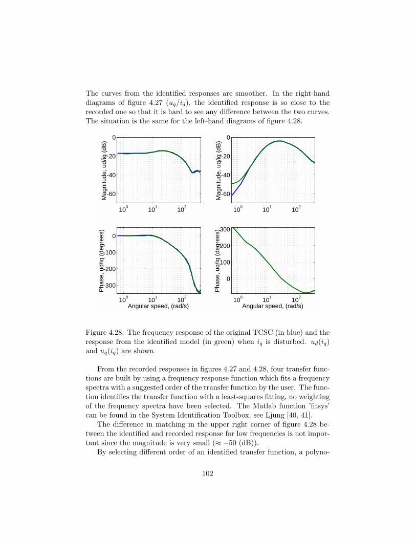
The curves from the identified responses are smoother. In the right-handdiagrams of figure 4.27 (uq/id), the identified response is so close to therecorded one so that it is hard to see any difference between the two curves.The situation is the same for the left-hand diagrams of figure 4.28.

100 101 102

-60

-40

-20

0

Mag

nitu

de, u

d/iq

(dB

)

100 101 102

-300

-200

-100

0

Pha

se, u

d/iq

(deg

rees

)

Angular speed, (rad/s)

100 101 102

-60

-40

-20

0

Mag

nitu

de, u

q/iq

(dB

)

100 101 102

0

100

200

300

Pha

se, u

q/iq

(deg

rees

)

Angular speed, (rad/s)

Figure 4.28: The frequency response of the original TCSC (in blue) and theresponse from the identified model (in green) when iq is disturbed. ud(iq)and uq(iq) are shown.

From the recorded responses in figures 4.27 and 4.28, four transfer func-tions are built by using a frequency response function which fits a frequencyspectra with a suggested order of the transfer function by the user. The func-tion identifies the transfer function with a least-squares fitting, no weightingof the frequency spectra have been selected. The Matlab function ’fitsys’can be found in the System Identification Toolbox, see Ljung [40, 41].

The difference in matching in the upper right corner of figure 4.28 be-tween the identified and recorded response for low frequencies is not impor-tant since the magnitude is very small (≈ −50 (dB)).

By selecting different order of an identified transfer function, a polyno-

102

mial with a response as close as possible to the recorded response can befound. This is done for each of the four transfer functions.

The identified responses demand at least a linear model of order 17. Fororders lower than 17, the matching between the identified and the recordedresponses in figures 4.27 and 4.28 are less.

Perturbing the d-component of the current

Figure 4.27 shows the frequency response of the TCSC when the d -compo-nent of the current has been disturbed with 10% of the steady-state valueof iline. The q-component of the current has remained equal to zero duringthe perturbation of the d -component.

The following two transfer functions have been identified for the TCSC,

G11(s) =∆ud(s)∆id(s)

= 0.0631(s + 0.4985)(s2 − 89.96s + 6.013 · 104)

(s + 751.8)(s2 + 126.6s + 5355)(4.18)

and

G21(s) =∆uq(s)∆id(s)

= −0.021901(s + 159)(s + 12.14)(s2 + 37.66s + 499.3)

·

·(s2 − 36.87s + 3.067 · 104)

(s2 + 167.7s + 1.884 · 104).

(4.19)

In equations (4.18) and (4.19) all poles (roots of the denominator) arein the left half plane.

In equation (4.18) there are right half plane zeros (roots of the numer-ator) at 45.0 ± j241.1 (1/s, rad/s). These zeros are probably of little sig-nificance since the frequency of them (38.4 (Hz)) is higher than what wewant to control/send into the linear model. The bandwidth we are inter-ested of is below this frequency. In general, zeros in the right half plane thatare ”far away” from the origin are often of little significance for control,Skogestad [76].

In equation (4.19) there are right half plane zeros at 18.4± j174.2 (1/s,rad/s). Also these zeros are probably of little significance since the frequencyof them (27.7 (Hz)) is high compared to what we want to control/send intothe linear model.

103

Perturbing the q-component of the current

Figure 4.28 shows the frequency response of the TCSC when the q-compo-nent of the current has been disturbed with 10% of the steady-state value ofiline. The d -component of the current has remained equal to the steady-statevalue during the perturbation of the q-component.

The following two transfer functions have been identified for the TCSC,

G12(s) =∆ud(s)∆iq(s)

= 0.014482(s + 439.5)(s + 11.39)(s2 + 50.94s + 754.6)

·

·(s2 − 109.5s + 5.188 · 104)

(s2 + 238.9s + 3.703 · 104)

(4.20)

and

G22(s) =∆uq(s)∆iq(s)

= 0.02088(s + 658.4)(s + 2.885)(s2 + 11.6s + 48.08)

·

· (s2 − 1.342s + 1.156)(s2 + 382s + 4.997 · 104)(s2 + 44.93s + 567.8)(s2 + 210.2s + 2.377 · 104)

.

(4.21)

In equations (4.20) and (4.21) all poles are in the left half plane.In equation (4.20) there are right half plane zeros at 54.8± j221.1 (1/s,

rad/s). These zeros are probably of little significance since the frequencyof them (35.2 (Hz)) is higher than what we want to control/send into thelinear model.

In equation (4.21) there are right half plane zeros at 0.67 ± j0.84 (1/s,rad/s). This is how our component has been identified and if the aim hadbeen to control the component in a certain way we could include this in adesign of a controller, but here the aim is to model the TCSC with a linearmodel and see if it behaves in the same way as our original TCSC model.Therefore we will include these zeros in the linear model.

4.8.4 A check of the linear model developed from frequencyanalysis

Before continuing we disturb the developed model in section 4.8 with thesame disturbance as we disturbed the original TCSC model in section 4.7when performing transient analysis. The results from the linear model areshown in figure 4.29 in red and the curves from the original TCSC model(earlier plotted in figure 4.9) are plotted in blue.

104

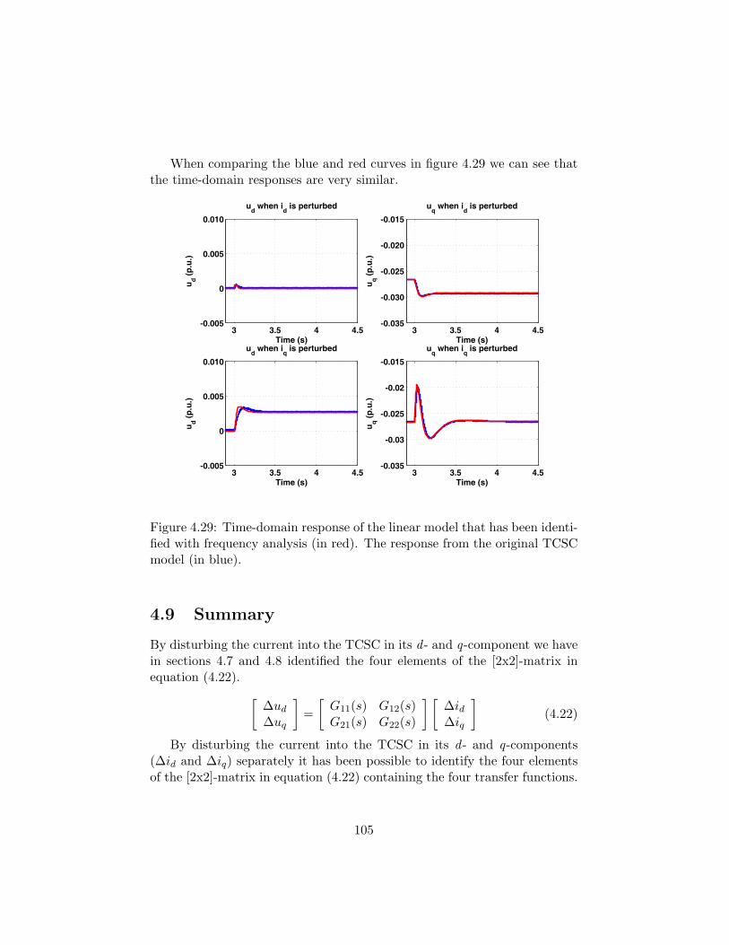
When comparing the blue and red curves in figure 4.29 we can see thatthe time-domain responses are very similar.

3 3.5 4 4.5-0.005

0

0.005

0.010

Time (s)

u d (p.u

.)

ud when i

d is perturbed

3 3.5 4 4.5-0.035

-0.030

-0.025

-0.020

-0.015

Time (s)

u q (p.u

.)

uq when i

d is perturbed

3 3.5 4 4.5-0.005

0

0.005

0.010

Time (s)

u d (p.u

.)

ud when i

q is perturbed

3 3.5 4 4.5-0.035

-0.03

-0.025

-0.02

-0.015

Time (s)

u q (p.u

.)

uq when i

q is perturbed

Figure 4.29: Time-domain response of the linear model that has been identi-fied with frequency analysis (in red). The response from the original TCSCmodel (in blue).

4.9 Summary

By disturbing the current into the TCSC in its d - and q-component we havein sections 4.7 and 4.8 identified the four elements of the [2x2]-matrix inequation (4.22). [

∆ud

∆uq

]=

[G11(s) G12(s)G21(s) G22(s)

] [∆id∆iq

](4.22)

By disturbing the current into the TCSC in its d - and q-components(∆id and ∆iq) separately it has been possible to identify the four elementsof the [2x2]-matrix in equation (4.22) containing the four transfer functions.

105

Our approach has been to disturb input by input. First we disturbedthe d -component of the current ∆id and studied the d - and q-components ofthe voltage ∆ud and ∆uq and with that, identified G11(s) and G21(s). Thenwe disturbed the q-component of the current ∆iq and studied the d - andq-components of the voltage ∆ud and ∆uq and with that identified G12(s)and G22(s). In the chapter we have seen the following differences when usingtwo methods to develop linear models,

• subsystem 12 for our model of the TCSC had different response whetherthe q-component of the current iq was increased or decreased,

• when developing the linear models we have used a first-order filter toreduce the amounts of harmonics for the methodology transient anal-ysis in section 4.7. When using the methodology frequency analysis insection 4.8 we used an Anti-aliasing filter,

• when using the methodology frequency analysis in section 4.8 we didnot have the possibility to observe the different response of ud of theTCSC for increases/decreases in iq, i.e., to observe the different re-sponse in subsystem 12.

106

Chapter 5

Interface to a linear model

In this chapter it is described how the created linear models are simulatedwith the rest of the power system. To use them, an interface system whichconnects them to the surrounding power system is utilized.

5.1 Introduction

The interface system described in this chapter is necessary to have since thelinear models have different response depending on if there is a change in thed - or q-component of the incoming current. Depending on if the incomingcurrent has an angle change or a magnitude change, the changes will betransformed to a local reference system where the current in a steady-statesituation is of pure d -component character.

The interface has to consider under which circumstances the developedlinear models are valid. The interface can be summarized as,

A) The developed linear models describe impact of changes from a steady-state operating point created by the interface system; and,

B) The steady state is defined as of pure d -component character withdifferent behavior of changes in d - and q-direction.

The interface system transforms a change in the magnitude of the in-coming current as a change in the d -component of the input to the linearmodel. A change in the angle of the incoming current is transformed to achange in the q-component of the input to the linear model. In a steady-state situation, the current through the linear model is zero.

107

It would be possible to let the current be of pure q-component characteror a mix of both d - and q-component but here as well as when we iden-tified the linear models in chapter 4 we have selected a pure d -componentcharacter.

The interface system is also slowly sliding from one steady state to an-other. This behavior means that the linear model, for the instant of adifference in magnitude of the incoming current or an angle difference in theincoming current, has a response which is timely for the dynamics of thereal TCSC. This feature of the interface makes the linear model having atimely response for subsequent disturbances.

The linear models that are created are developed in the dq0 -coordinatesystem, i.e., the so-called Park’s transformation, see Park [49]. All simula-tions are done in the instantaneous value mode, i.e., instantaneous valuesof phase voltages and phase currents can be shown although they are cal-culated in a dq0 -coordinate system. As mentioned in chapter 3 there is no0 -component in the studied system. Therefore we exclude the 0 -componentof the currents and voltages. So from now on we simply write dq-coordinatesystem.

The linear models are representing a small-signal model of the powersystem component and represent the dynamic behaviour of the componentfrom a steady state. The steady state of the power system component isrepresented by the steady-state model in figure 5.1. The sum of the responsefrom the steady-state model and the linear model is the total response fromthe studied power system component.

5.2 Coordinate system

The coordinate system for the linear models is representing a local dq-coordinate system which is standing still in a steady-state situation. Be-tween the local coordinate system and the surrounding power system existsan interface which is described in this chapter.

One advantage of representing a power system simulation with instanta-neous values using the dq-coordinated frame is that the dq-frame is standingstill in steady state and is slowly varying close to a steady-state situation,i.e., the currents and voltages are in the dq-frame varying very slow com-pared to phase quantities which are in a steady state in instantaneous valuemode varying sinusoidal with the power frequency of the network.

108

5.3 Interface system

In figure 5.1, the interface system is shown. Observe that the interface sys-tem is only used when simulations are done with the linear models. Simula-tions with the original TCSC model are done without the interface system.

The input signals to the interface system are the three-phase currentsshown in the upper left part of figure 5.1. The output signal is the complex-valued signal U that is shown in the right part of figure 5.1.

The interface system is connected both to the linear model of the TCSCas well as to the steady-state model of the TCSC as in figure 5.1. Thelinear model and the steady-state model may represent any power systemcomponent but is in the thesis representing a TCSC.

Bold lines in figure 5.1 represent complex-valued quantities.The input signal i(t) consists of a real and an imaginary part, ire(t) and

iim(t) and is defined as in equation (5.1) below,

i(t) = ire(t) + jiim(t) =23(ia(t) + ej 2π

3 · ib(t) + e−j 2π3 · ic(t)) (5.1)

where ia(t), ib(t), and ic(t) are instantaneous phase currents, scalars.This transformation keeps the magnitude of the phase quantities during

symmetrical conditions, i.e., the length of the space vector (the magnitudesof ire(t) and iim(t)) is identical with the magnitudes of the phase quantitiesia(t), ib(t), and ic(t), Angquist [88].

Equation (5.1) is often referred to as the space-vector approach, Kovacs[34] and i(t) is a current vector for the three instantaneous phase-currents,see also Nee [47] and Angquist [88]. ia(t), ib(t), and ic(t) in figure 5.1 are theincoming instantaneous phase-currents from the surrounding power system.

As mentioned in chapter 3, the 0 -component is not necessary to includein the simulations and as a function of that, transformation (5.1) is possible.The three-phase currents are represented in the dq-frame of the surroundingpower system, see id + jiq in figure 5.1.

The angle θ in figure 5.1 is the angle of the steady-state current ISS . θis calculated in the block diagram 6 ISS and is used as an input signal totwo of the block diagrams in figure 5.1. The signal ωref is the rotor speedof the reference machine in the power system.

The real and imaginary parts of i(t); ire(t) and iim(t), are in steadystate sinus formed with the power frequency of the network and containinformation about all three phases as shown in the following three equations.

109

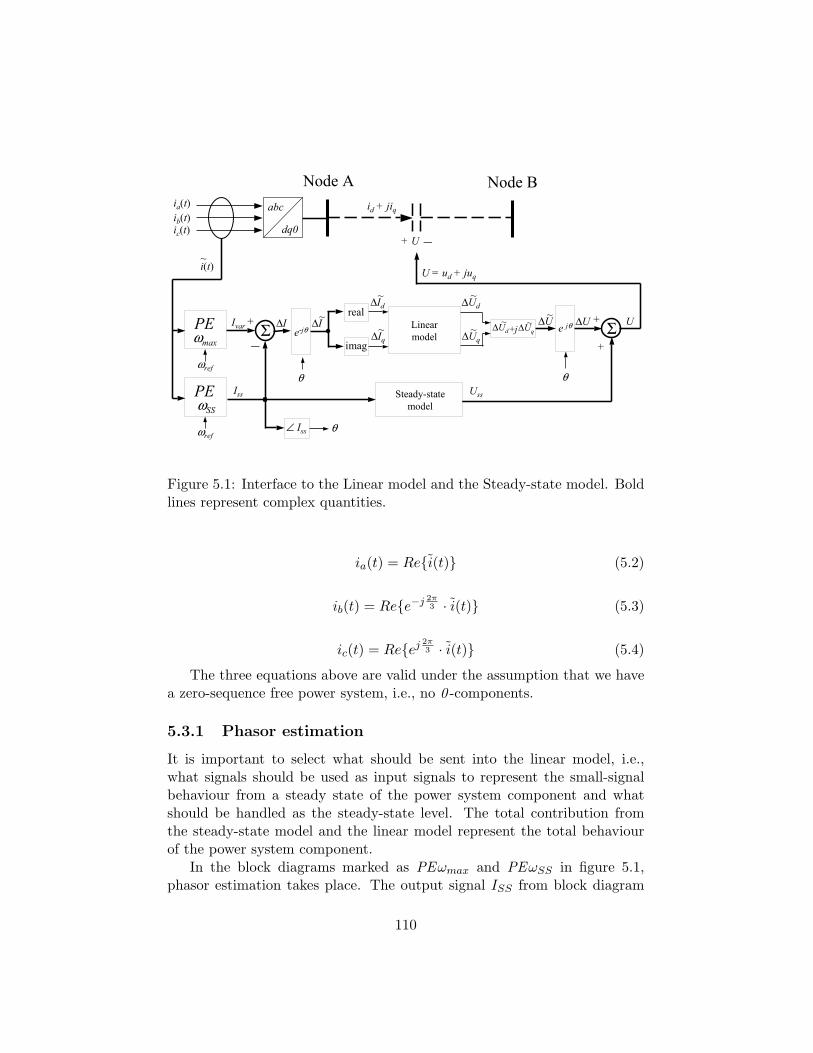
PEωmax

Iss

Linearmodel

+

ia(t)ib(t)ic(t)

i(t)~

θ∠ Iss

θθ

Ivar

_Σ ∆I ∆I ~e-jθ

∆Id ~

∆Iq ~

∆Ud ~

∆Uq ~ e jθ

Uss

∆U ~ +Σ

+

∆U U

abc

dq0+ U _

id + jiq

U = ud + juq

Node A Node B

real

imag+j∆Ud

~ ∆Uq ~

Steady-statemodel

PEωSS

ωref

ωref

Figure 5.1: Interface to the Linear model and the Steady-state model. Boldlines represent complex quantities.

ia(t) = Rei(t) (5.2)

ib(t) = Ree−j 2π3 · i(t) (5.3)

ic(t) = Reej 2π3 · i(t) (5.4)

The three equations above are valid under the assumption that we havea zero-sequence free power system, i.e., no 0 -components.

5.3.1 Phasor estimation

It is important to select what should be sent into the linear model, i.e.,what signals should be used as input signals to represent the small-signalbehaviour from a steady state of the power system component and whatshould be handled as the steady-state level. The total contribution fromthe steady-state model and the linear model represent the total behaviourof the power system component.

In the block diagrams marked as PEωmax and PEωSS in figure 5.1,phasor estimation takes place. The output signal ISS from block diagram

110

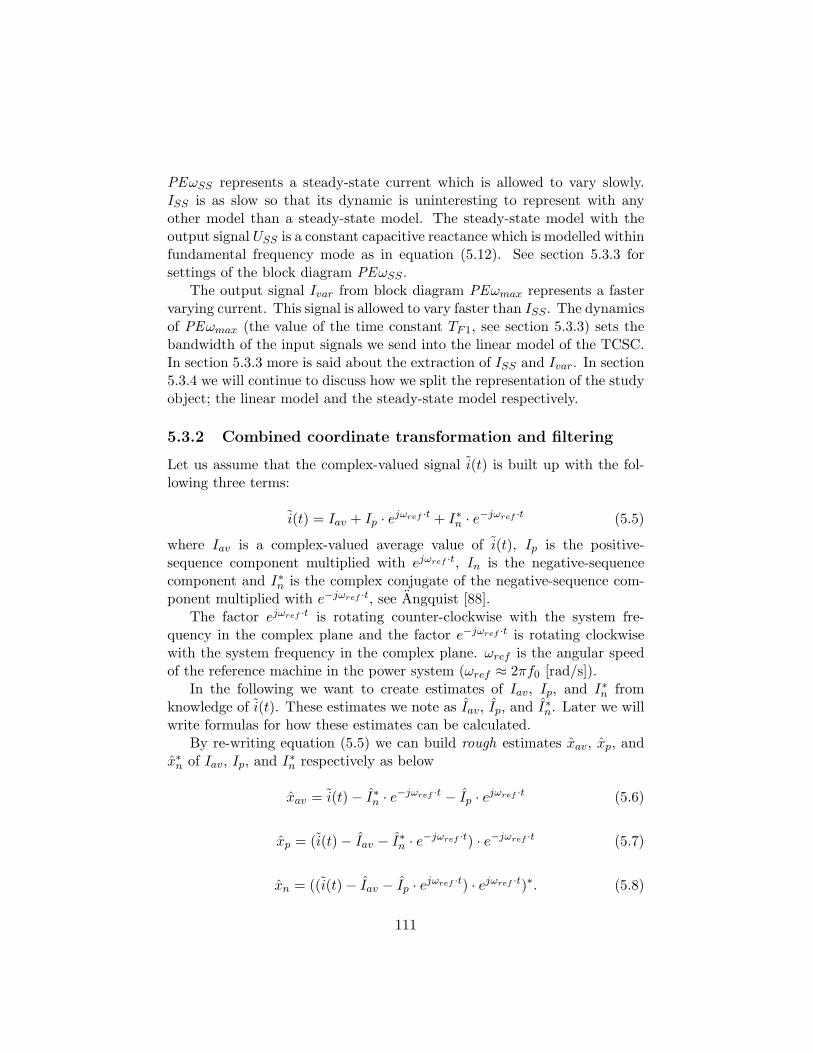
PEωSS represents a steady-state current which is allowed to vary slowly.ISS is as slow so that its dynamic is uninteresting to represent with anyother model than a steady-state model. The steady-state model with theoutput signal USS is a constant capacitive reactance which is modelled withinfundamental frequency mode as in equation (5.12). See section 5.3.3 forsettings of the block diagram PEωSS .

The output signal Ivar from block diagram PEωmax represents a fastervarying current. This signal is allowed to vary faster than ISS . The dynamicsof PEωmax (the value of the time constant TF1, see section 5.3.3) sets thebandwidth of the input signals we send into the linear model of the TCSC.In section 5.3.3 more is said about the extraction of ISS and Ivar. In section5.3.4 we will continue to discuss how we split the representation of the studyobject; the linear model and the steady-state model respectively.

5.3.2 Combined coordinate transformation and filtering

Let us assume that the complex-valued signal i(t) is built up with the fol-lowing three terms:

i(t) = Iav + Ip · ejωref ·t + I∗n · e−jωref ·t (5.5)

where Iav is a complex-valued average value of i(t), Ip is the positive-sequence component multiplied with ejωref ·t, In is the negative-sequencecomponent and I∗n is the complex conjugate of the negative-sequence com-ponent multiplied with e−jωref ·t, see Angquist [88].

The factor ejωref ·t is rotating counter-clockwise with the system fre-quency in the complex plane and the factor e−jωref ·t is rotating clockwisewith the system frequency in the complex plane. ωref is the angular speedof the reference machine in the power system (ωref ≈ 2πf0 [rad/s]).

In the following we want to create estimates of Iav, Ip, and I∗n fromknowledge of i(t). These estimates we note as Iav, Ip, and I∗n. Later we willwrite formulas for how these estimates can be calculated.

By re-writing equation (5.5) we can build rough estimates xav, xp, andx∗n of Iav, Ip, and I∗n respectively as below

xav = i(t)− I∗n · e−jωref ·t − Ip · ejωref ·t (5.6)

xp = (i(t)− Iav − I∗n · e−jωref ·t) · e−jωref ·t (5.7)

xn = ((i(t)− Iav − Ip · ejωref ·t) · ejωref ·t)∗. (5.8)

111

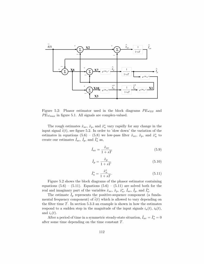
+i(t)~

_Σ

+

_

Σ+

_ Σ

+

_ Σ

e-jω t ref1

1+sT

1

1+sT

X7

X10 X1

+

_Σ

1

1+sT X2

X6

e-jω t ref

e jω t ref

e jω t ref

X3

In^

Iav^

Ip^

xav^

xp^

xn^* *

Figure 5.2: Phasor estimator used in the block diagrams PEωSS andPEωmax in figure 5.1. All signals are complex-valued.

The rough estimates xav, xp, and x∗n vary rapidly for any change in theinput signal i(t), see figure 5.2. In order to ’slow down’ the variation of theestimates in equations (5.6) – (5.8) we low-pass filter xav, xp, and x∗n tocreate our estimates Iav, Ip, and I∗n as,

Iav =xav

1 + sT(5.9)

Ip =xp

1 + sT(5.10)

I∗n =x∗n

1 + sT. (5.11)

Figure 5.2 shows the block diagrams of the phasor estimator containingequations (5.6) – (5.11). Equations (5.6) – (5.11) are solved both for thereal and imaginary part of the variables xav, xp, x∗n, Iav, Ip, and I∗n.

The estimate Ip represents the positive-sequence component (a funda-mental frequency component) of i(t) which is allowed to vary depending onthe filter time T . In section 5.3.3 an example is shown in how the estimatesrespond to a sudden step in the magnitude of the input signals ia(t), ib(t),and ic(t).

After a period of time in a symmetric steady-state situation, Iav = I∗n = 0after some time depending on the time constant T .

112

0 0.01 0.02 0.03 0.04 0.05 0.06 0.07 0.08 0.09 0.10

0.2

0.4

0.6

0.8

1

Time (s)

|I av| ,

|Ip| ,

|In| (

p.u.

)

|Ip|

|In|

|Iav

|

Figure 5.3: Time-domain response to a sudden step in the magnitudes ofthe three input signals ia(t), ib(t), and ic(t) from 0 to 1, see figure 5.1. ia(t),ib(t), and ic(t) are symmetric.

5.3.3 Time constants to filter ISS and Ivar

To calculate ISS and Ivar we use the phasor estimator introduced in sections5.3.1, 5.3.2, and figure 5.2. When we estimate ISS we set a time constantTF2 (indicated as T in figure 5.2) to a value between 0.5 < TF2 < 2.0 (s),Angquist [87]. The output signal Ip from the phasor estimator in figure 5.2then represents ISS , a slow phasor of i(t).

ISS is also indicated in figure 5.1 as the output signal from the blockdiagram PEωSS .

By using the same phasor estimator but with a faster time constant Twe can estimate the quantity Ip but now allow it to vary faster. The timeconstant TF1 is here set to a value in the interval 0.004 < TF1 < 0.4 (s),Angquist [87]. The output signal Ip from the phasor estimator in figure 5.2then represents Ivar.

Ivar is representing a faster phasor of i(t) than ISS . Ivar can also befound in figure 5.1 as the output signal from block diagram PEωmax.

The difference between Ivar and ISS is later sent into the linear modelto represent the input signals to the small-signal model of the TCSC, seesection 5.3.4.

113

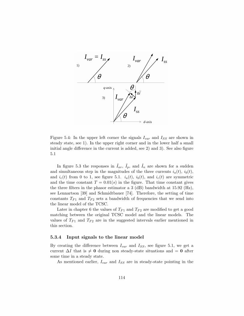
θ

θIss

Ivar ∆I∆I~

d-axis

q-axis

3)

θ

IssIvar Ivar = Iss

θ

1) 2)

Figure 5.4: In the upper left corner the signals Ivar and ISS are shown insteady state, see 1). In the upper right corner and in the lower half a smallinitial angle difference in the current is added, see 2) and 3). See also figure5.1

In figure 5.3 the responses in Iav, Ip, and In are shown for a suddenand simultaneous step in the magnitudes of the three currents ia(t), ib(t),and ic(t) from 0 to 1, see figure 5.1. ia(t), ib(t), and ic(t) are symmetricand the time constant T = 0.01(s) in the figure. That time constant givesthe three filters in the phasor estimator a 3 (dB) bandwidth at 15.92 (Hz),see Lennartson [39] and Schmidtbauer [74]. Therefore, the setting of timeconstants TF1 and TF2 sets a bandwidth of frequencies that we send intothe linear model of the TCSC.

Later in chapter 6 the values of TF1 and TF2 are modified to get a goodmatching between the original TCSC model and the linear models. Thevalues of TF1 and TF2 are in the suggested intervals earlier mentioned inthis section.

5.3.4 Input signals to the linear model

By creating the difference between Ivar and ISS , see figure 5.1, we get acurrent ∆I that is 6= 0 during non steady-state situations and = 0 aftersome time in a steady state.

As mentioned earlier, Ivar and ISS are in steady-state pointing in the

114

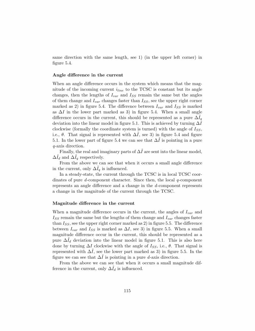
same direction with the same length, see 1) (in the upper left corner) infigure 5.4.

Angle difference in the current

When an angle difference occurs in the system which means that the mag-nitude of the incoming current iline to the TCSC is constant but its anglechanges, then the lengths of Ivar and ISS remain the same but the anglesof them change and Ivar changes faster than ISS , see the upper right cornermarked as 2) in figure 5.4. The difference between Ivar and ISS is markedas ∆I in the lower part marked as 3) in figure 5.4. When a small angledifference occurs in the current, this should be represented as a pure ∆Iq

deviation into the linear model in figure 5.1. This is achieved by turning ∆Iclockwise (formally the coordinate system is turned) with the angle of ISS ,i.e., θ. That signal is represented with ∆I, see 3) in figure 5.4 and figure5.1. In the lower part of figure 5.4 we can see that ∆I is pointing in a pureq-axis direction.

Finally, the real and imaginary parts of ∆I are sent into the linear model,∆Id and ∆Iq respectively.

From the above we can see that when it occurs a small angle differencein the current, only ∆Iq is influenced.

In a steady-state, the current through the TCSC is in local TCSC coor-dinates of pure d -component character. Since then, the local q-componentrepresents an angle difference and a change in the d -component representsa change in the magnitude of the current through the TCSC.

Magnitude difference in the current

When a magnitude difference occurs in the current, the angles of Ivar andISS remain the same but the lengths of them change and Ivar changes fasterthan ISS , see the upper right corner marked as 2) in figure 5.5. The differencebetween Ivar and ISS is marked as ∆I, see 3) in figure 5.5. When a smallmagnitude difference occur in the current, this should be represented as apure ∆Id deviation into the linear model in figure 5.1. This is also heredone by turning ∆I clockwise with the angle of ISS , i.e., θ. That signal isrepresented with ∆I, see the lower part marked as 3) in figure 5.5. In thefigure we can see that ∆I is pointing in a pure d -axis direction.

From the above we can see that when it occurs a small magnitude dif-ference in the current, only ∆Id is influenced.

115

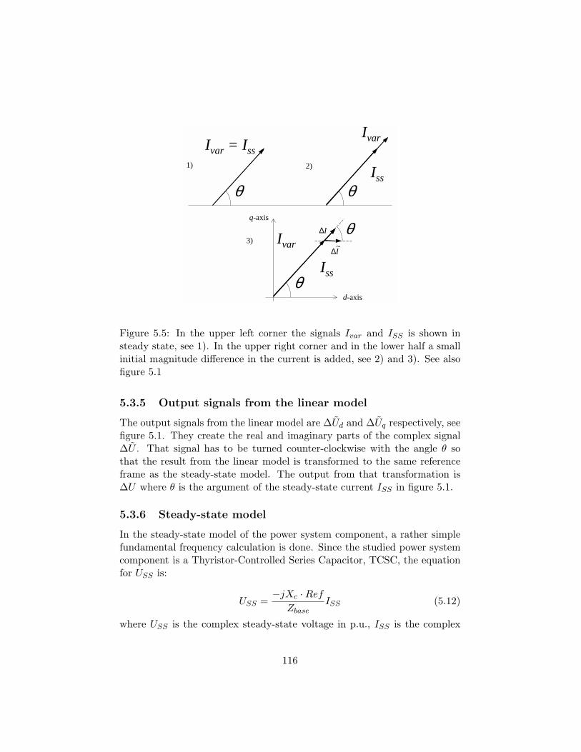
θIss

Ivar Ivar = Iss

θ

θ

θIss

Ivar ∆I

∆I~

d-axis

q-axis

1) 2)

3)

Figure 5.5: In the upper left corner the signals Ivar and ISS is shown insteady state, see 1). In the upper right corner and in the lower half a smallinitial magnitude difference in the current is added, see 2) and 3). See alsofigure 5.1

5.3.5 Output signals from the linear model

The output signals from the linear model are ∆Ud and ∆Uq respectively, seefigure 5.1. They create the real and imaginary parts of the complex signal∆U . That signal has to be turned counter-clockwise with the angle θ sothat the result from the linear model is transformed to the same referenceframe as the steady-state model. The output from that transformation is∆U where θ is the argument of the steady-state current ISS in figure 5.1.

5.3.6 Steady-state model

In the steady-state model of the power system component, a rather simplefundamental frequency calculation is done. Since the studied power systemcomponent is a Thyristor-Controlled Series Capacitor, TCSC, the equationfor USS is:

USS =−jXc ·Ref

ZbaseISS (5.12)

where USS is the complex steady-state voltage in p.u., ISS is the complex

116

steady-state current in p.u., Xc is the capacitive reactance of the capacitor inΩ, Ref is a reference value specified for the TCSC which fundamental capac-itive reactance the TCSC should produce, and Zbase is the base impedanceof the component. (Zbase = Ubase

2

Sbase, where Ubase is the phase-to-phase rms

base voltage of the TCSC-nodes and Sbase is the three-phase base power ofthe network).

The sum of USS and ∆U in figure 5.1 represents the total response fromthe power system component, see U in figure 5.1.

The d - and q-components of U express the voltage drop of the TCSCand represents the dynamic behaviour of the TCSC.

5.4 Summary

In this chapter an interface has been introduced which aim is to connect thelinear models to the surrounding power system.

The interface system is slowly sliding from one steady state to another.This feature of the interface makes the linear model having a timely responsefor subsequent disturbances.

Earlier in publications of the subject of the thesis, see Persson [55, 58,59, 61, 62] another interface system has been used. However, in chapter 6 itcan be seen that the interface system developed here in the thesis providesa better agreement between the developed linear models and the originalTCSC model compared to the earlier publications.

117

118

Chapter 6

Time-domain simulations

This chapter compares time-domain simulations with the original TCSCmodel and the created linear models. First, we tune the interface systembetween the linear models and the rest of the power system and then com-parisons are made for three different cases. The event in the first case isin the same range as was used when the linear models were developed inchapter 4. The second case contains a larger disturbance and the third casesimulates a disturbance wherein the power system is in another operatingpoint.

6.1 Background

To control the accuracy of the linear models of the TCSC, comparisonsare made with the linear models and the original TCSC model. Since thelinear models have been developed under the assumptions for being validfor small-signal perturbations, the perturbations cannot be too large. Theassumption on which a linearization is built is that in a narrow interval ofthe input signals, the component behaves linearly. Therefore, the createdlinear models are valid for such small disturbances and the accuracy maydecrease when larger disturbances are applied.

6.2 Settings of the interface system

Before we can start using our linear models and validate them we have to setthe filter constants of the interface system that was introduced in chapter 5.To do this we return to our stiff identification system that was used earlierin chapter 4.

119

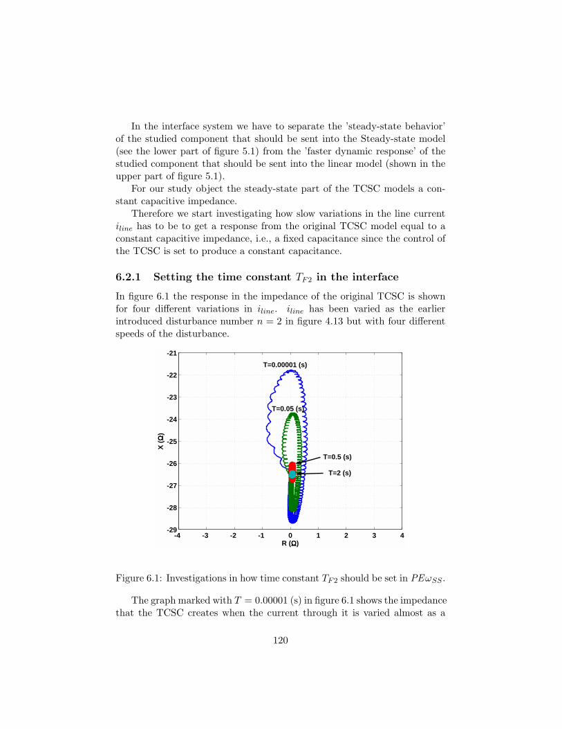
In the interface system we have to separate the ’steady-state behavior’of the studied component that should be sent into the Steady-state model(see the lower part of figure 5.1) from the ’faster dynamic response’ of thestudied component that should be sent into the linear model (shown in theupper part of figure 5.1).

For our study object the steady-state part of the TCSC models a con-stant capacitive impedance.

Therefore we start investigating how slow variations in the line currentiline has to be to get a response from the original TCSC model equal to aconstant capacitive impedance, i.e., a fixed capacitance since the control ofthe TCSC is set to produce a constant capacitance.

6.2.1 Setting the time constant TF2 in the interface

In figure 6.1 the response in the impedance of the original TCSC is shownfor four different variations in iline. iline has been varied as the earlierintroduced disturbance number n = 2 in figure 4.13 but with four differentspeeds of the disturbance.

-4 -3 -2 -1 0 1 2 3 4-29

-28

-27

-26

-25

-24

-23

-22

-21

R (ΩΩΩΩ)

X ( ΩΩ ΩΩ

)

T=0.00001 (s)

T=0.05 (s)

T=0.5 (s)

T=2 (s)

Figure 6.1: Investigations in how time constant TF2 should be set in PEωSS .

The graph marked with T = 0.00001 (s) in figure 6.1 shows the impedancethat the TCSC creates when the current through it is varied almost as a

120

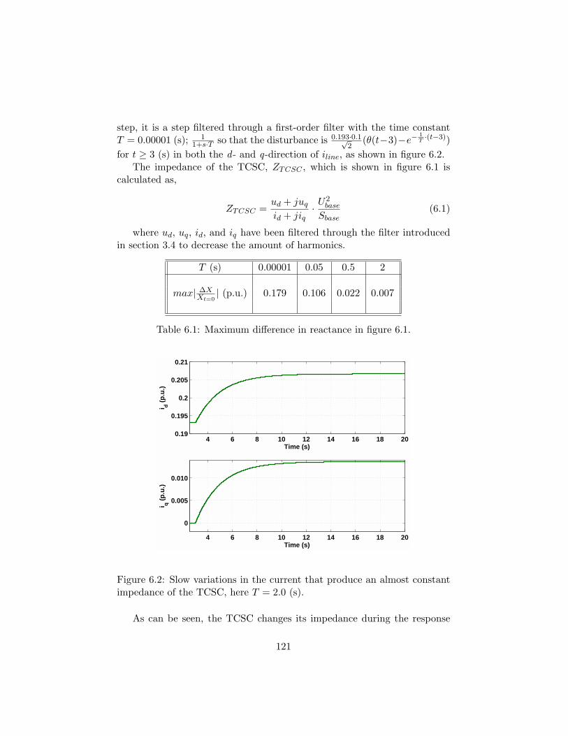
step, it is a step filtered through a first-order filter with the time constantT = 0.00001 (s); 1

1+s·T so that the disturbance is 0.193·0.1√2

(θ(t−3)−e−1T·(t−3))

for t ≥ 3 (s) in both the d - and q-direction of iline, as shown in figure 6.2.The impedance of the TCSC, ZTCSC , which is shown in figure 6.1 is

calculated as,

ZTCSC =ud + juq

id + jiq·U2

base

Sbase(6.1)

where ud, uq, id, and iq have been filtered through the filter introducedin section 3.4 to decrease the amount of harmonics.

T (s) 0.00001 0.05 0.5 2

max| ∆XXt=0

| (p.u.) 0.179 0.106 0.022 0.007

Table 6.1: Maximum difference in reactance in figure 6.1.

4 6 8 10 12 14 16 18 200.19

0.195

0.2

0.205

0.21

Time (s)

i d (p.u

.)

4 6 8 10 12 14 16 18 20

0

0.005

0.010

Time (s)

i q (p.u

.)

Figure 6.2: Slow variations in the current that produce an almost constantimpedance of the TCSC, here T = 2.0 (s).

As can be seen, the TCSC changes its impedance during the response

121

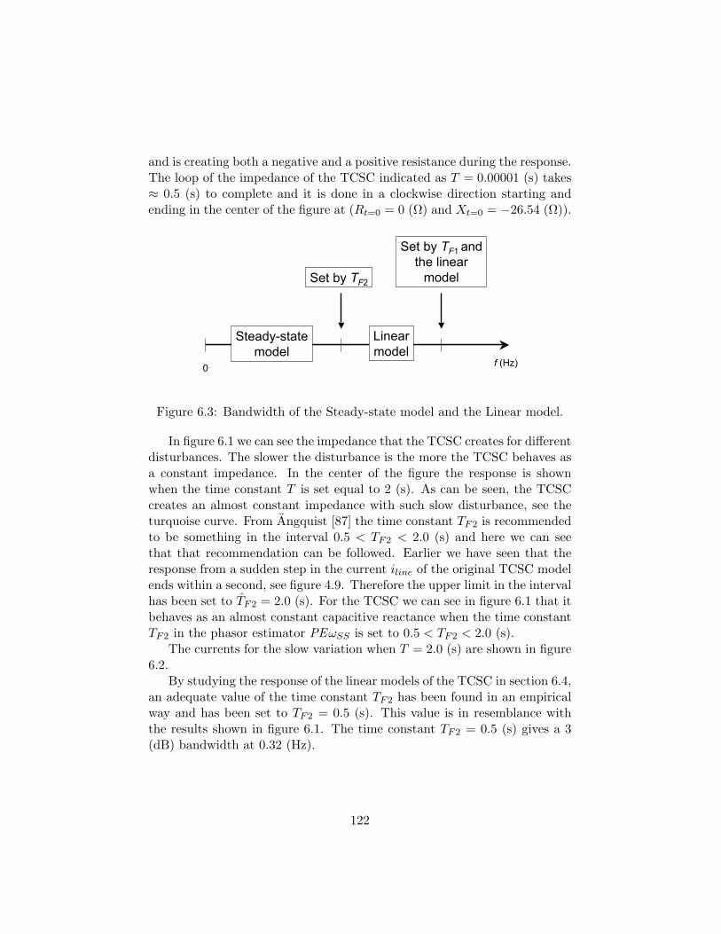
and is creating both a negative and a positive resistance during the response.The loop of the impedance of the TCSC indicated as T = 0.00001 (s) takes≈ 0.5 (s) to complete and it is done in a clockwise direction starting andending in the center of the figure at (Rt=0 = 0 (Ω) and Xt=0 = −26.54 (Ω)).

0

Set by TF2

f (Hz)

Steady-statemodel

Linearmodel

Set by TF1 and the linear

model

Figure 6.3: Bandwidth of the Steady-state model and the Linear model.

In figure 6.1 we can see the impedance that the TCSC creates for differentdisturbances. The slower the disturbance is the more the TCSC behaves asa constant impedance. In the center of the figure the response is shownwhen the time constant T is set equal to 2 (s). As can be seen, the TCSCcreates an almost constant impedance with such slow disturbance, see theturquoise curve. From Angquist [87] the time constant TF2 is recommendedto be something in the interval 0.5 < TF2 < 2.0 (s) and here we can seethat that recommendation can be followed. Earlier we have seen that theresponse from a sudden step in the current iline of the original TCSC modelends within a second, see figure 4.9. Therefore the upper limit in the intervalhas been set to TF2 = 2.0 (s). For the TCSC we can see in figure 6.1 that itbehaves as an almost constant capacitive reactance when the time constantTF2 in the phasor estimator PEωSS is set to 0.5 < TF2 < 2.0 (s).

The currents for the slow variation when T = 2.0 (s) are shown in figure6.2.

By studying the response of the linear models of the TCSC in section 6.4,an adequate value of the time constant TF2 has been found in an empiricalway and has been set to TF2 = 0.5 (s). This value is in resemblance withthe results shown in figure 6.1. The time constant TF2 = 0.5 (s) gives a 3(dB) bandwidth at 0.32 (Hz).

122

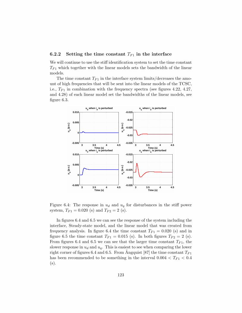
6.2.2 Setting the time constant TF1 in the interface

We will continue to use the stiff identification system to set the time constantTF1 which together with the linear models sets the bandwidth of the linearmodels.

The time constant TF1 in the interface system limits/decreases the amo-unt of high frequencies that will be sent into the linear models of the TCSC,i.e., TF1 in combination with the frequency spectra (see figures 4.22, 4.27,and 4.28) of each linear model set the bandwidths of the linear models, seefigure 6.3.

3 3.5 4 4.5-0.005

0

0.005

0.010

Time (s)

u d (p.u

.)

ud when i

d is perturbed

3 3.5 4 4.5-0.035

-0.03

-0.025

-0.02

-0.015

Time (s)

u q (p.u

.)

uq when i

d is perturbed

3 3.5 4 4.5-0.005

0

0.005

0.010

Time (s)

u d (p.u

.)

ud when i

q is perturbed

3 3.5 4 4.5-0.035

-0.03

-0.025

-0.02

-0.015

Time (s)

u q (p.u

.)

uq when i

q is perturbed

Figure 6.4: The response in ud and uq for disturbances in the stiff powersystem, TF1 = 0.020 (s) and TF2 = 2 (s).

In figures 6.4 and 6.5 we can see the response of the system including theinterface, Steady-state model, and the linear model that was created fromfrequency analysis. In figure 6.4 the time constant TF1 = 0.020 (s) and infigure 6.5 the time constant TF1 = 0.015 (s). In both figures TF2 = 2 (s).From figures 6.4 and 6.5 we can see that the larger time constant TF1, theslower response in ud and uq. This is easiest to see when comparing the lowerright corner of figures 6.4 and 6.5. From Angquist [87] the time constant TF1

has been recommended to be something in the interval 0.004 < TF1 < 0.4(s).

123

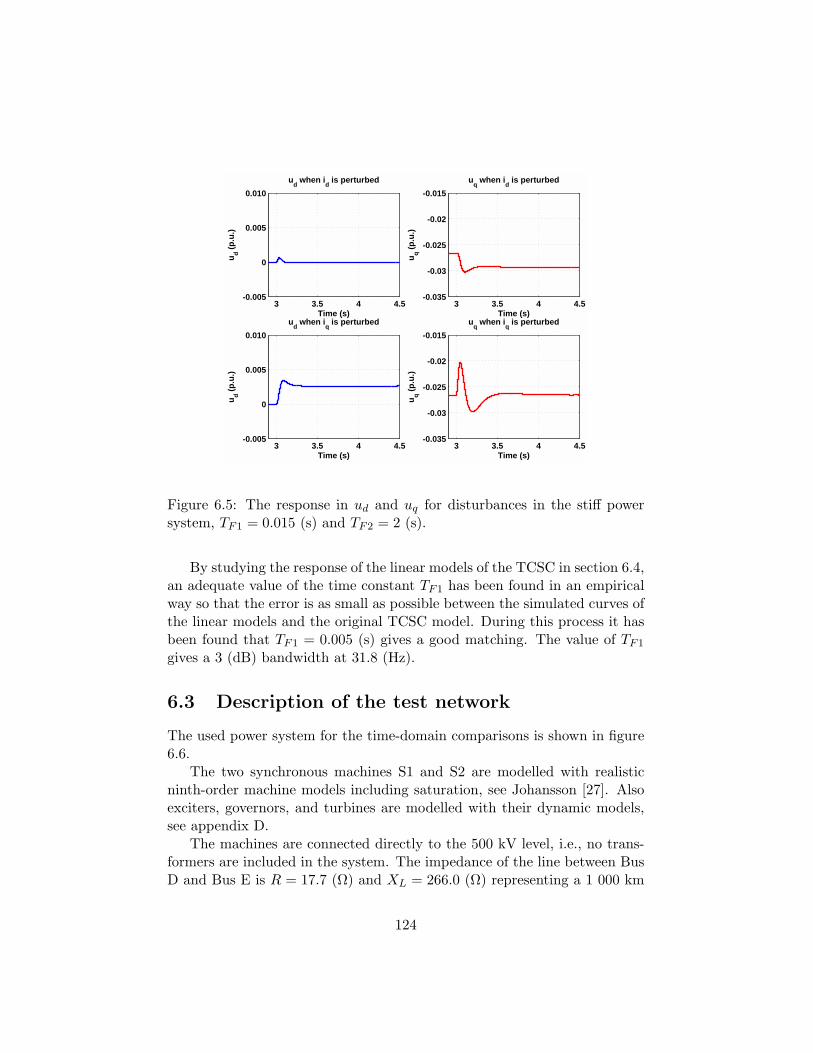
3 3.5 4 4.5-0.005

0

0.005

0.010

Time (s)

u d (p.u

.)

ud when i

d is perturbed

3 3.5 4 4.5-0.035

-0.03

-0.025

-0.02

-0.015

Time (s)

u q (p.u

.)

uq when i

d is perturbed

3 3.5 4 4.5-0.005

0

0.005

0.010

Time (s)

u d (p.u

.)

ud when i

q is perturbed

3 3.5 4 4.5-0.035

-0.03

-0.025

-0.02

-0.015

Time (s)

u q (p.u

.)

uq when i

q is perturbed

Figure 6.5: The response in ud and uq for disturbances in the stiff powersystem, TF1 = 0.015 (s) and TF2 = 2 (s).

By studying the response of the linear models of the TCSC in section 6.4,an adequate value of the time constant TF1 has been found in an empiricalway so that the error is as small as possible between the simulated curves ofthe linear models and the original TCSC model. During this process it hasbeen found that TF1 = 0.005 (s) gives a good matching. The value of TF1

gives a 3 (dB) bandwidth at 31.8 (Hz).

6.3 Description of the test network

The used power system for the time-domain comparisons is shown in figure6.6.

The two synchronous machines S1 and S2 are modelled with realisticninth-order machine models including saturation, see Johansson [27]. Alsoexciters, governors, and turbines are modelled with their dynamic models,see appendix D.

The machines are connected directly to the 500 kV level, i.e., no trans-formers are included in the system. The impedance of the line between BusD and Bus E is R = 17.7 (Ω) and XL = 266.0 (Ω) representing a 1 000 km

124

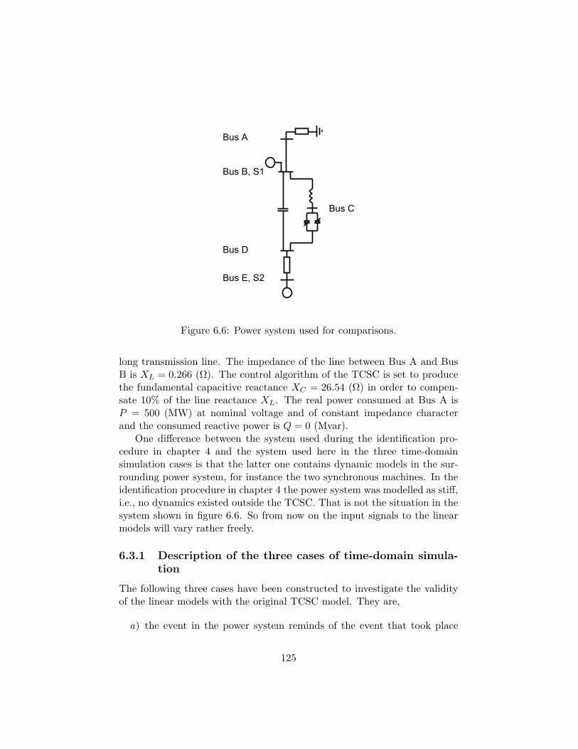
Bus A

Bus B, S1

Bus D

Bus E, S2

Bus C

Figure 6.6: Power system used for comparisons.

long transmission line. The impedance of the line between Bus A and BusB is XL = 0.266 (Ω). The control algorithm of the TCSC is set to producethe fundamental capacitive reactance XC = 26.54 (Ω) in order to compen-sate 10% of the line reactance XL. The real power consumed at Bus A isP = 500 (MW) at nominal voltage and of constant impedance characterand the consumed reactive power is Q = 0 (Mvar).

One difference between the system used during the identification pro-cedure in chapter 4 and the system used here in the three time-domainsimulation cases is that the latter one contains dynamic models in the sur-rounding power system, for instance the two synchronous machines. In theidentification procedure in chapter 4 the power system was modelled as stiff,i.e., no dynamics existed outside the TCSC. That is not the situation in thesystem shown in figure 6.6. So from now on the input signals to the linearmodels will vary rather freely.

6.3.1 Description of the three cases of time-domain simula-tion

The following three cases have been constructed to investigate the validityof the linear models with the original TCSC model. They are,

a) the event in the power system reminds of the event that took place

125

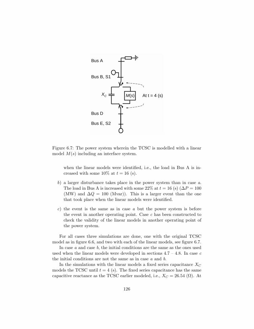
Bus A

Bus B, S1

Bus D

Bus E, S2

At t = 4 (s)M(s)XC

Figure 6.7: The power system wherein the TCSC is modelled with a linearmodel M(s) including an interface system.

when the linear models were identified, i.e., the load in Bus A is in-creased with some 10% at t = 16 (s).

b) a larger disturbance takes place in the power system than in case a.The load in Bus A is increased with some 22% at t = 16 (s) (∆P = 100(MW) and ∆Q = 100 (Mvar)). This is a larger event than the onethat took place when the linear models were identified.

c) the event is the same as in case a but the power system is beforethe event in another operating point. Case c has been constructed tocheck the validity of the linear models in another operating point ofthe power system.

For all cases three simulations are done, one with the original TCSCmodel as in figure 6.6, and two with each of the linear models, see figure 6.7.

In case a and case b, the initial conditions are the same as the ones usedused when the linear models were developed in sections 4.7 – 4.8. In case cthe initial conditions are not the same as in case a and b.

In the simulations with the linear models a fixed series capacitance XC

models the TCSC until t = 4 (s). The fixed series capacitance has the samecapacitive reactance as the TCSC earlier modeled, i.e., XC = 26.54 (Ω). At

126

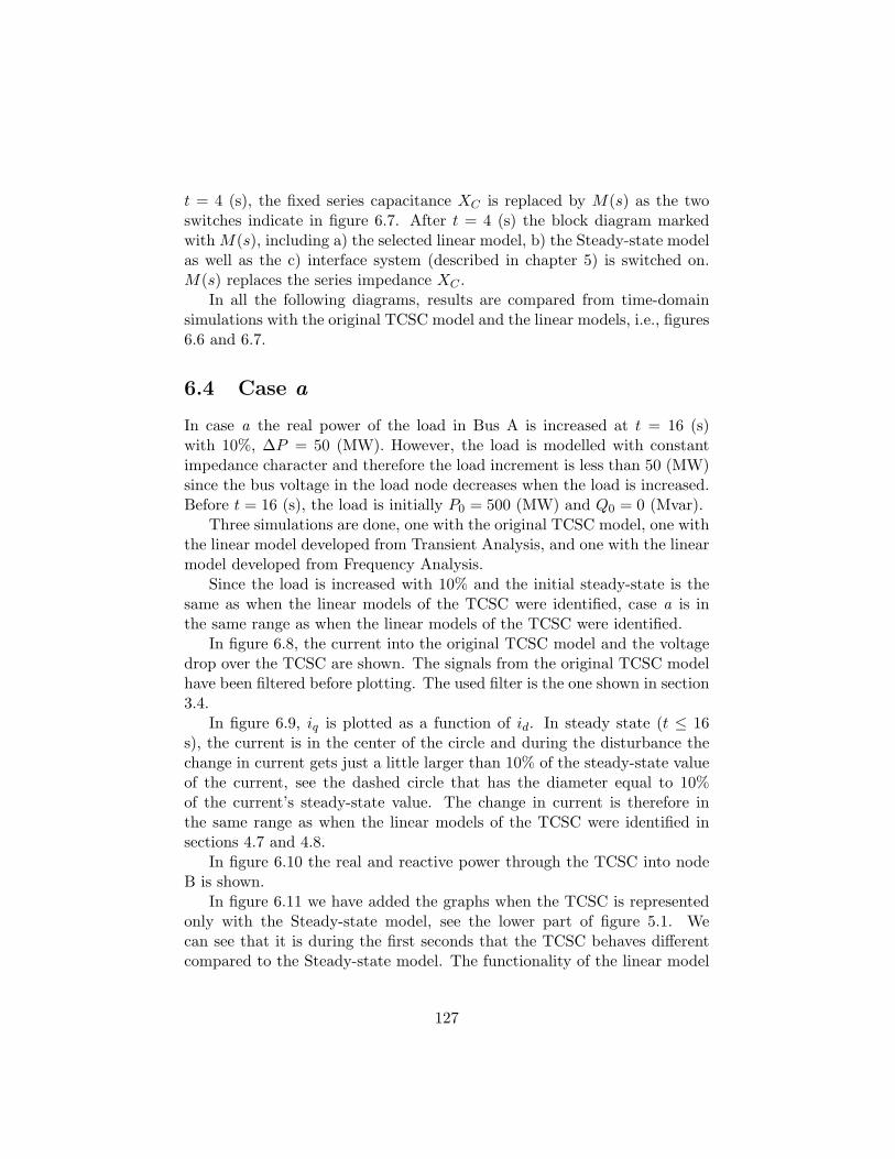
t = 4 (s), the fixed series capacitance XC is replaced by M(s) as the twoswitches indicate in figure 6.7. After t = 4 (s) the block diagram markedwith M(s), including a) the selected linear model, b) the Steady-state modelas well as the c) interface system (described in chapter 5) is switched on.M(s) replaces the series impedance XC .

In all the following diagrams, results are compared from time-domainsimulations with the original TCSC model and the linear models, i.e., figures6.6 and 6.7.

6.4 Case a

In case a the real power of the load in Bus A is increased at t = 16 (s)with 10%, ∆P = 50 (MW). However, the load is modelled with constantimpedance character and therefore the load increment is less than 50 (MW)since the bus voltage in the load node decreases when the load is increased.Before t = 16 (s), the load is initially P0 = 500 (MW) and Q0 = 0 (Mvar).

Three simulations are done, one with the original TCSC model, one withthe linear model developed from Transient Analysis, and one with the linearmodel developed from Frequency Analysis.

Since the load is increased with 10% and the initial steady-state is thesame as when the linear models of the TCSC were identified, case a is inthe same range as when the linear models of the TCSC were identified.

In figure 6.8, the current into the original TCSC model and the voltagedrop over the TCSC are shown. The signals from the original TCSC modelhave been filtered before plotting. The used filter is the one shown in section3.4.

In figure 6.9, iq is plotted as a function of id. In steady state (t ≤ 16s), the current is in the center of the circle and during the disturbance thechange in current gets just a little larger than 10% of the steady-state valueof the current, see the dashed circle that has the diameter equal to 10%of the current’s steady-state value. The change in current is therefore inthe same range as when the linear models of the TCSC were identified insections 4.7 and 4.8.

In figure 6.10 the real and reactive power through the TCSC into nodeB is shown.

In figure 6.11 we have added the graphs when the TCSC is representedonly with the Steady-state model, see the lower part of figure 5.1. Wecan see that it is during the first seconds that the TCSC behaves differentcompared to the Steady-state model. The functionality of the linear model

127

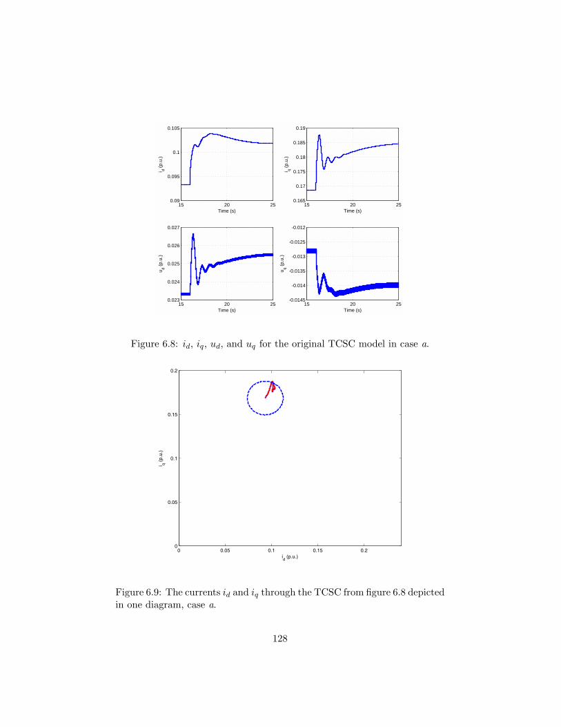
15 20 250.09

0.095

0.1

0.105

Time (s)

i d (p.u

.)

15 20 250.165

0.17

0.175

0.18

0.185

0.19

Time (s)

i q (p.u

.)

15 20 250.023

0.024

0.025

0.026

0.027

Time (s)

u d (p.u

.)

15 20 25-0.0145

-0.014

-0.0135

-0.013

-0.0125

-0.012

Time (s)

u q (p.u

.)

Figure 6.8: id, iq, ud, and uq for the original TCSC model in case a.

0 0.05 0.1 0.15 0.20

0.05

0.1

0.15

0.2

id (p.u.)

i q (p.u

.)

Figure 6.9: The currents id and iq through the TCSC from figure 6.8 depictedin one diagram, case a.

128

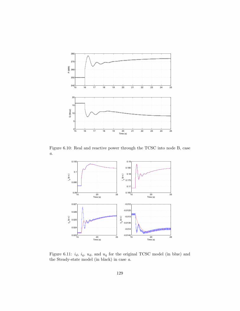
15 16 17 18 19 20 21 22 23 24 25240

250

260

270

280

P (M

W)

15 16 17 18 19 20 21 22 23 24 250

5

10

15

20

Time (s)

Q (M

var)

Figure 6.10: Real and reactive power through the TCSC into node B, casea.

15 20 250.09

0.095

0.1

0.105

Time (s)

i d (p.u

.)

15 20 250.165

0.17

0.175

0.18

0.185

0.19

Time (s)

i q (p.u

.)

15 20 250.023

0.024

0.025

0.026

0.027

Time (s)

u d (p.u

.)

15 20 25-0.0145

-0.014

-0.0135

-0.013

-0.0125

-0.012

Time (s)

u q (p.u

.)

Figure 6.11: id, iq, ud, and uq for the original TCSC model (in blue) andthe Steady-state model (in black) in case a.

129

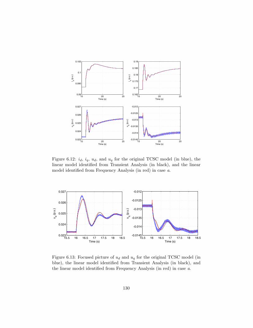
15 20 250.09

0.095

0.1

0.105

Time (s)

i d (p.u

.)

15 20 250.165

0.17

0.175

0.18

0.185

0.19

Time (s)

i q (p.u

.)

15 20 250.023

0.024

0.025

0.026

0.027

Time (s)

u d (p.u

.)

15 20 25-0.0145

-0.014

-0.0135

-0.013

-0.0125

-0.012

Time (s)

u q (p.u

.)

Figure 6.12: id, iq, ud, and uq for the original TCSC model (in blue), thelinear model identified from Transient Analysis (in black), and the linearmodel identified from Frequency Analysis (in red) in case a.

15.5 16 16.5 17 17.5 18 18.50.023

0.024

0.025

0.026

0.027

Time (s)

u d (p.u

.)

15.5 16 16.5 17 17.5 18 18.5-0.0145

-0.014

-0.0135

-0.013

-0.0125

-0.012

Time (s)

u q (p.u

.)

Figure 6.13: Focused picture of ud and uq for the original TCSC model (inblue), the linear model identified from Transient Analysis (in black), andthe linear model identified from Frequency Analysis (in red) in case a.

130

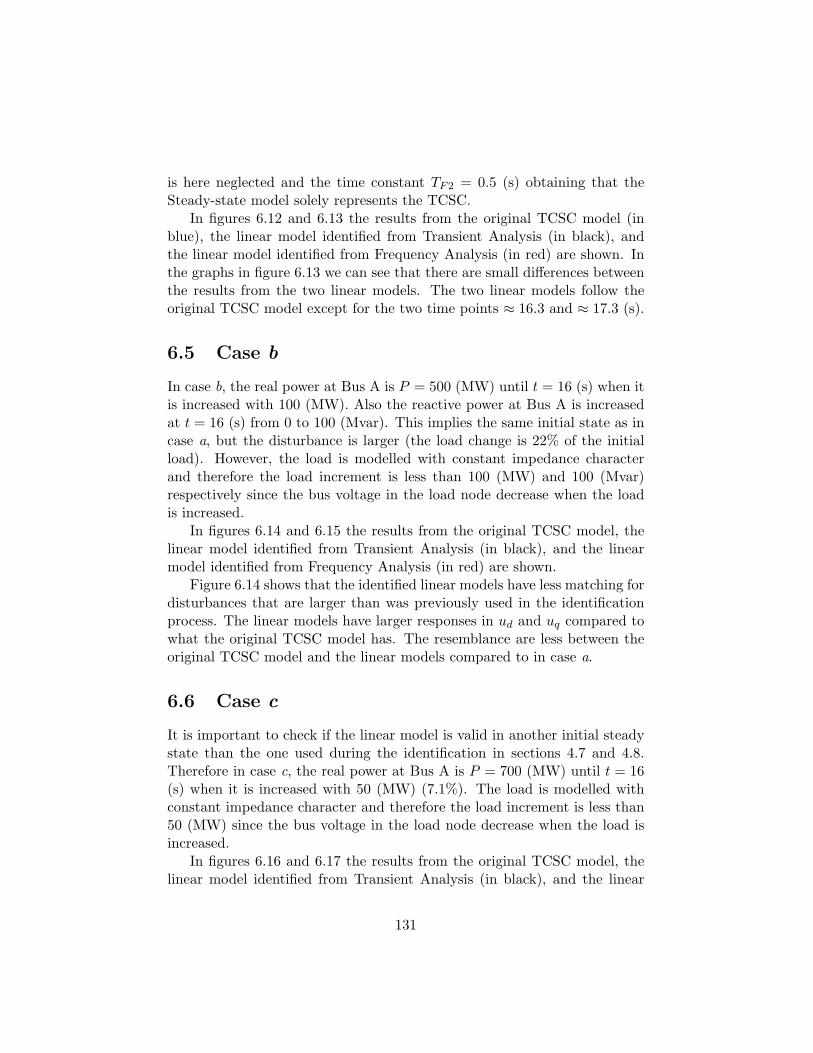
is here neglected and the time constant TF2 = 0.5 (s) obtaining that theSteady-state model solely represents the TCSC.

In figures 6.12 and 6.13 the results from the original TCSC model (inblue), the linear model identified from Transient Analysis (in black), andthe linear model identified from Frequency Analysis (in red) are shown. Inthe graphs in figure 6.13 we can see that there are small differences betweenthe results from the two linear models. The two linear models follow theoriginal TCSC model except for the two time points ≈ 16.3 and ≈ 17.3 (s).

6.5 Case b

In case b, the real power at Bus A is P = 500 (MW) until t = 16 (s) when itis increased with 100 (MW). Also the reactive power at Bus A is increasedat t = 16 (s) from 0 to 100 (Mvar). This implies the same initial state as incase a, but the disturbance is larger (the load change is 22% of the initialload). However, the load is modelled with constant impedance characterand therefore the load increment is less than 100 (MW) and 100 (Mvar)respectively since the bus voltage in the load node decrease when the loadis increased.

In figures 6.14 and 6.15 the results from the original TCSC model, thelinear model identified from Transient Analysis (in black), and the linearmodel identified from Frequency Analysis (in red) are shown.

Figure 6.14 shows that the identified linear models have less matching fordisturbances that are larger than was previously used in the identificationprocess. The linear models have larger responses in ud and uq compared towhat the original TCSC model has. The resemblance are less between theoriginal TCSC model and the linear models compared to in case a.

6.6 Case c

It is important to check if the linear model is valid in another initial steadystate than the one used during the identification in sections 4.7 and 4.8.Therefore in case c, the real power at Bus A is P = 700 (MW) until t = 16(s) when it is increased with 50 (MW) (7.1%). The load is modelled withconstant impedance character and therefore the load increment is less than50 (MW) since the bus voltage in the load node decrease when the load isincreased.

In figures 6.16 and 6.17 the results from the original TCSC model, thelinear model identified from Transient Analysis (in black), and the linear

131

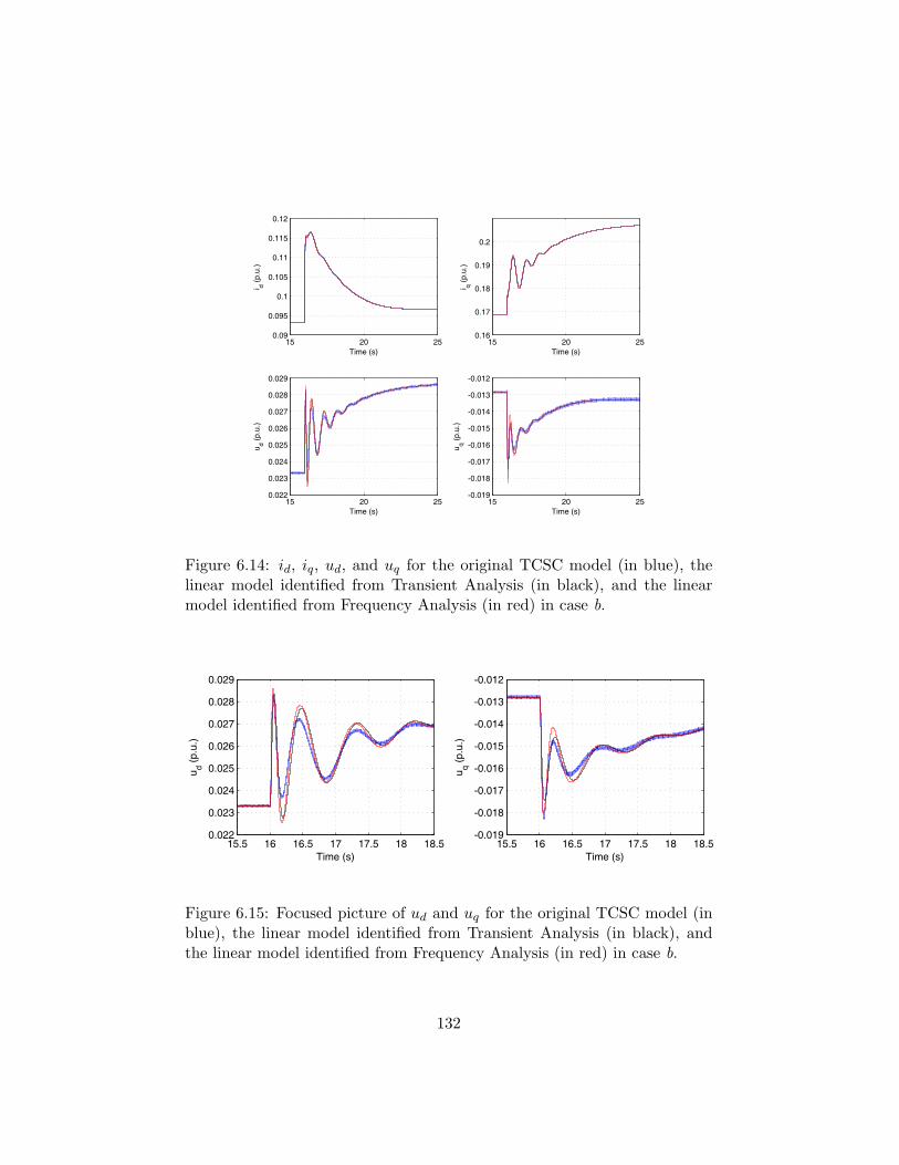
15 20 250.09

0.095

0.1

0.105

0.11

0.115

0.12

Time (s)

i d (p.u

.)

15 20 250.16

0.17

0.18

0.19

0.2

Time (s)

i q (p.u

.)

15 20 250.022

0.023

0.024

0.025

0.026

0.027

0.028

0.029

Time (s)

u d (p.u

.)

15 20 25-0.019

-0.018

-0.017

-0.016

-0.015

-0.014

-0.013

-0.012

Time (s)

u q (p.u

.)

Figure 6.14: id, iq, ud, and uq for the original TCSC model (in blue), thelinear model identified from Transient Analysis (in black), and the linearmodel identified from Frequency Analysis (in red) in case b.

15.5 16 16.5 17 17.5 18 18.50.022

0.023

0.024

0.025

0.026

0.027

0.028

0.029

Time (s)

u d (p.u

.)

15.5 16 16.5 17 17.5 18 18.5-0.019

-0.018

-0.017

-0.016

-0.015

-0.014

-0.013

-0.012

Time (s)

u q (p.u

.)

Figure 6.15: Focused picture of ud and uq for the original TCSC model (inblue), the linear model identified from Transient Analysis (in black), andthe linear model identified from Frequency Analysis (in red) in case b.

132

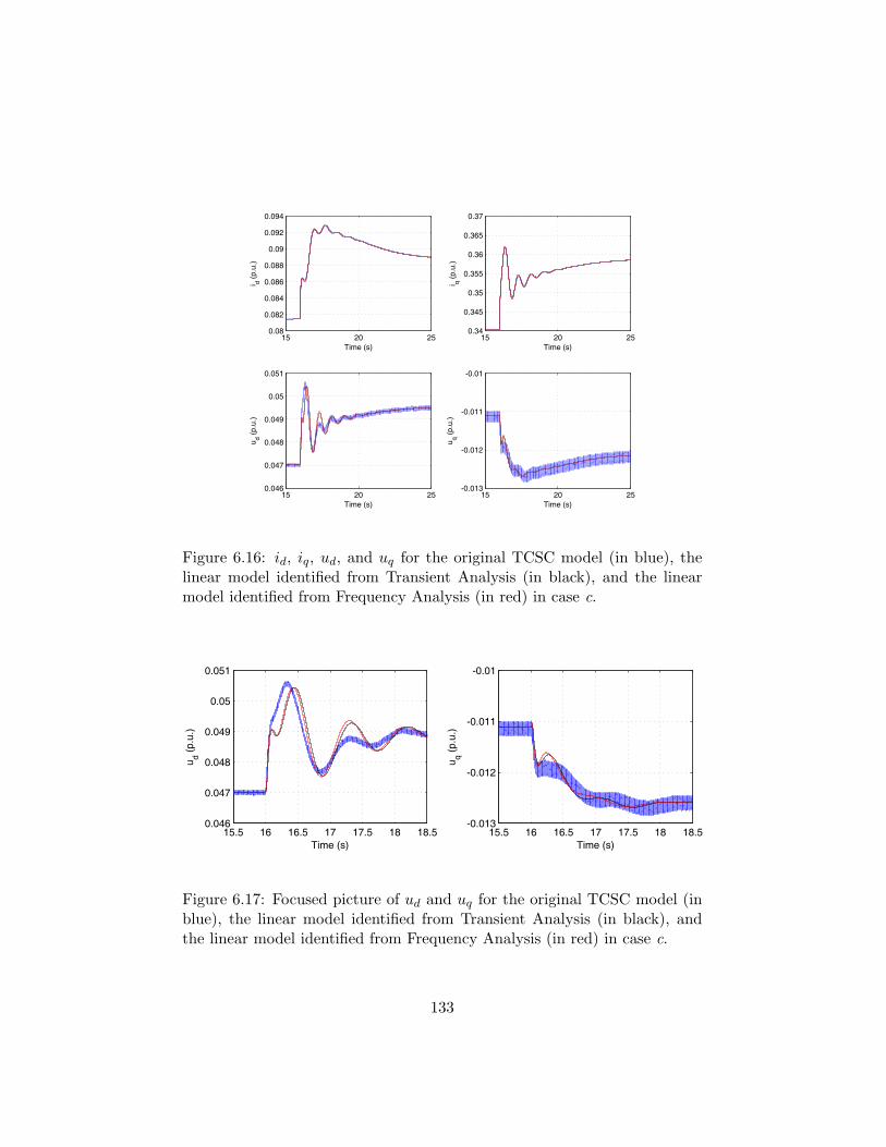
15 20 250.08

0.082

0.084

0.086

0.088

0.09

0.092

0.094

Time (s)

i d (p.u

.)

15 20 250.34

0.345

0.35

0.355

0.36

0.365

0.37

Time (s)

i q (p.u

.)

15 20 250.046

0.047

0.048

0.049

0.05

0.051

Time (s)

u d (p.u

.)

15 20 25-0.013

-0.012

-0.011

-0.01

Time (s)

u q (p.u

.)

Figure 6.16: id, iq, ud, and uq for the original TCSC model (in blue), thelinear model identified from Transient Analysis (in black), and the linearmodel identified from Frequency Analysis (in red) in case c.

15.5 16 16.5 17 17.5 18 18.50.046

0.047

0.048

0.049

0.05

0.051

Time (s)

u d (p.u

.)

15.5 16 16.5 17 17.5 18 18.5-0.013

-0.012

-0.011

-0.01

Time (s)

u q (p.u

.)

Figure 6.17: Focused picture of ud and uq for the original TCSC model (inblue), the linear model identified from Transient Analysis (in black), andthe linear model identified from Frequency Analysis (in red) in case c.

133

model identified from Frequency Analysis (in red) are shown.Figure 6.14 shows that the identified linear models have less matching in

another working point that was previously used in the identification process.The resemblance are less between the original TCSC model and the linearmodels compared to in case a.

6.7 Summary

In this chapter we have set the filter constants of the interface system thatwas earlier introduced in chapter 5.

In the interface system we have separated the ’steady-state behavior’ ofthe TCSC from the ’faster dynamic response’. The ’steady-state behavior’of the TCSC was sent into the Steady-state model and the ’faster dynamicresponse’ was sent into the linear models. The steady-state part of theTCSC models a constant capacitive impedance.

The created linear models have been compared in time-domain simula-tions. Both of the linear models provide results which are similar to theoriginal TCSC model although the linear models showed more resemblancein case a than in cases b and c.

The responses from the linear models are close in the three cases. Thissimilarity between the linear models have earlier been shown in the models’frequency responses, see figures 4.22, 4.27, and 4.28 as well as in the time-domain responses shown in figures 4.19, 4.20, and 4.29.

Time-domain simulations with the linear models are much faster to per-form compared to time-domain simulations with the original TCSC model.The simulations with the linear models demand a few per cent of physicaltime compared to the simulations with the original TCSC model.

In time-domain simulations with the linear models, the harmonics thatwere included in simulations with the original TCSC model are not presentsince the bandwidth of the linear models is reduced. The slow dynamic ofthe original TCSC model is however represented by the linear models.

The interface system developed in the thesis provides good agreementbetween the developed linear models and the original TCSC model. Inearlier publications carried out within this thesis work another interfacesystem has been used. The one used herein is better than the previous oneused in Persson [55].

The interface developed in this thesis contains a ’sliding’ effect, i.e., theinterface is slowly moving to a new steady state at the same time as it isseparating two bandwidths; allowing frequencies up to one bandwidth to be

134

sent into the Steady-state model of the component and frequencies up to asecond bandwidth to be sent into the linear model representing the ’fasterdynamic response’ of the component. The interface in Persson [55] did notcontain any of these characteristics. It was a static interface, valid only forone steady state and did not separate any bandwidths.

135

136

Chapter 7

Small-signal stability analysis

This chapter contains comparisons of small-signal stability analysis (linearanalysis) of the two linear models earlier developed in chapter 4.

7.1 Background

Linear models allow for the application of small-signal stability analysis tech-niques (linear analysis) to complement the information obtained from non-linear time-domain simulations and often allow for a better understandingof the dynamic characteristic of the system than that obtained from the in-spection of time-domain simulations alone. Although the non-linear natureof a power system must be recognized, in many cases a linearized system rep-resentation allows for a more efficient means of analysis, Sanchez-Gasca [73].

When modelling the TCSC in detail it contains power electronics (thyris-tors) that switches in and out several times for each cycle. As a result of theswitchings and the TCSC’s non-linear control algorithm, the TCSC behavesnon-linear. A time-domain model of a TCSC can be made very accurateand is essential for studying large disturbances in the vicinity of the TCSC.However, these models are not suitable for small-signal stability analysis(linear analysis) of a power system including a TCSC, Othman [48].

If we would perform a linearization of the power system including thedetailed original TCSC model we would have problems with the thyristorswitchings and the change in setup of differential equations of the TCSCand the result from the linearization would be hard to interpret. The lin-earization would depend on the actual thyristor status as well as the actualstatus of the control algorithm. Eigenvalues would not occur consistent be-tween different time points of linearization within the same steady state.

137

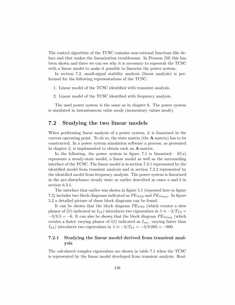
The control algorithm of the TCSC contains non-rational functions like de-lays and that makes the linearization troublesome. In Persson [58] this hasbeen shown and there we can see why it is necessary to represent the TCSCwith a linear model to make it possible to linearize the power system.

In section 7.2, small-signal stability analysis (linear analysis) is per-formed for the following representations of the TCSC:

1. Linear model of the TCSC identified with transient analysis.

2. Linear model of the TCSC identified with frequency analysis.

The used power system is the same as in chapter 6. The power systemis simulated in instantaneous value mode (momentary values mode).

7.2 Studying the two linear models

When performing linear analysis of a power system, it is linearized in thecurrent operating point. To do so, the state matrix (the A-matrix) has to beconstructed. In a power system simulation software a process, as presentedin chapter 2, is implemented to obtain such an A-matrix.

In the following, the power system in figure 7.1 is linearized. M(s)represents a steady-state model, a linear model as well as the surroundinginterface of the TCSC. The linear model is in section 7.2.1 represented by theidentified model from transient analysis and in section 7.2.2 represented bythe identified model from frequency analysis. The power system is linearizedin the pre-disturbance steady state as earlier described in cases a and b insection 6.3.1.

The interface that earlier was shown in figure 5.1 (repeated here in figure7.2) includes two block diagrams indicated as PEωSS and PEωmax. In figure5.2 a detailed picture of these block diagrams can be found.

It can be shown that the block diagram PEωSS (which creates a slowphasor of i(t) indicated as ISS) introduces two eigenvalues in λ ≈ −3/TF2 =−3/0.5 = −6. It can also be shown that the block diagram PEωmax (whichcreates a faster varying phasor of i(t) indicated as Ivar, varying faster thanISS) introduces two eigenvalues in λ ≈ −3/TF1 = −3/0.005 = −600.

7.2.1 Studying the linear model derived from transient anal-ysis

The calculated complex eigenvalues are shown in table 7.1 when the TCSCis represented by the linear model developed from transient analysis. Real-

138

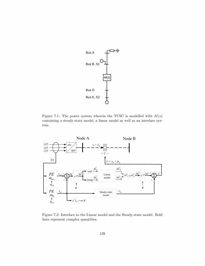
Bus A

Bus B, S1

Bus D

Bus E, S2

M(s)

Figure 7.1: The power system wherein the TCSC is modelled with M(s)containing a steady-state model, a linear model as well as an interface sys-tem.

PEωmax

Iss

Linearmodel

+

ia(t)ib(t)ic(t)

i(t)~

θ∠ Iss

θθ

Ivar

_Σ ∆I ∆I ~e-jθ

∆Id ~

∆Iq ~

∆Ud ~

∆Uq ~ e jθ

Uss

∆U ~ +Σ

+

∆U U

abc

dq0+ U _

id + jiq

U = ud + juq

Node A Node B

real

imag+j∆Ud

~ ∆Uq ~

Steady-statemodel

PEωSS

ωref

ωref

Figure 7.2: Interface to the Linear model and the Steady-state model. Boldlines represent complex quantities.

139

λ σ ± jω [1/s, Hz] Commentλ1,2 −1.30± j1.13 Inter-area oscillationλ3,4 −17.04± j0.27 Already found in phasor modeλ5,6 −35.28± j0.04 Already found in phasor modeλ7,8 −3.93± j0.19 Already found in phasor modeλ9,10 −1.41± j0.24 Already found in phasor modeλ11,12 −0.56± j0.06 Already found in phasor modeλ13,14 −2.54± j0.59 Already found in phasor modeλ15,16 −25.47± j5.14 Pole from G11(s)λ17,18 −14.33± j3.73 Pole from G21(s)λ19,20 −10.55± j2.18 Pole from G12(s)λ21,22 −8.09± j1.37 Pole from G22(s)λ23,24 −26.59± j5.21 Pole from G22(s)λ25,26 −24.09± j60.00 f0

λ27,28 −16.85± j60.09 f0

Table 7.1: Complex poles with real part greater than −200 with the linearmodel identified from transient analysis. Eigenvalues λ1 – λ14 are found inphasor mode when the TCSC is modelled as a constant series capacitor.

valued eigenvalues are not listed. When calculating the eigenvalues, theanalytical linearization (AL) method is used.

The eigenvalue-pair λ1,2 in table 7.1 is an inter-area oscillation. Aftera disturbance, power oscillates between the two areas of the power systemwith the frequency 1.13 (Hz) during the recovery of the power system. TheTCSC interconnects the two areas. That oscillation can be observed in time-domain simulations of the power system, see figures for case a – case c insections 6.4 - 6.6.

Eigenvalues λ3 – λ12 in table 7.1 occur when the synchronous machinesinclude exciters, i.e., when the synchronous machines are modelled withoutexciters these eigenvalues do not exist. Eigenvalue-pair λ13,14 occurs whenthe synchronous machines include turbines and governors.

The less damped eigenvalue-pair in table 7.1 is λ11,12. However, theimaginary part of that eigenvalue-pair is very small and therefore impossibleto detect in a time-domain simulation.

Eigenvalues λ15 – λ24 are derived from the poles of the transfer functionsof the linear model that were identified in section 4.7.

Eigenvalue-pairs λ25,26 and λ27,28 come from the system’s power fre-quency and are generated from the actual implementation of the interface

140

together with the linear models.The total number of eigenvalues is 57 where 10 comes from the linear

model of the TCSC.

7.2.2 Studying the linear model derived from frequency anal-ysis

The calculated complex eigenvalues are shown in table 7.2 when the TCSCis represented by the linear model developed from frequency analysis. Real-valued eigenvalues are not listed.

Eigenvalues λ1 – λ14 occur also in this subsection as in subsection 7.2.1.See subsection 7.2.1 for comments about them.

Eigenvalues λ15 – λ30 are derived from the poles of the transfer functionsof the linear model that were identified in section 4.8.

The total number of eigenvalues is 64 where 17 comes from the linearmodel of the TCSC.

Also the real-valued pole derived from G11(s), see equation (4.18), isincluded but not shown in table 7.2.

Eigenvalue-pairs λ31,32 is a result of a fusion of two real-valued eigen-values. Earlier in section 7.2.1 this eigenvalue-pair constituted of two real-valued eigenvalues λ = −14.63 and λ = −18.70.

7.3 Summary

In this chapter, two linear models of a TCSC have been utilized. The small-signal stability analysis (linear analysis) of the studied power system havebeen made in instantaneous value mode.

In Persson [58] is has been shown how troublesome it is to perform linearanalysis using the original TCSC model. By replacing the original TCSCmodel with a linear model, linear analysis is possible to perform.

By comparing table 7.1 and 7.2 we can see that the result from linearanalysis of the system is the same, independent of which linear model thatis used; the eigenvalues λ1 – λ14 are in both tables consistent.

Among the listed eigenvalues we can find the poles from the linear modelswhich have been identified from the original TCSC model.

When representing the TCSC with the linear models, all eigenvaluesexist, no matter when linear analysis is done in a steady-state. This is incontradiction with linear analysis performed with the original TCSC model.

141

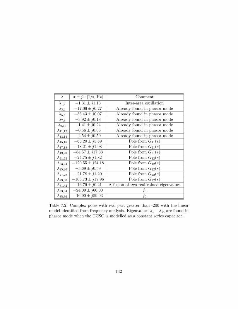
λ σ ± jω [1/s, Hz] Commentλ1,2 −1.31± j1.13 Inter-area oscillationλ3,4 −17.06± j0.27 Already found in phasor modeλ5,6 −35.43± j0.07 Already found in phasor modeλ7,8 −3.92± j0.18 Already found in phasor modeλ9,10 −1.41± j0.24 Already found in phasor modeλ11,12 −0.56± j0.06 Already found in phasor modeλ13,14 −2.54± j0.59 Already found in phasor modeλ15,16 −63.20± j5.89 Pole from G11(s)λ17,18 −18.21± j1.98 Pole from G21(s)λ19,20 −84.57± j17.33 Pole from G21(s)λ21,22 −24.75± j1.82 Pole from G12(s)λ23,24 −120.55± j24.18 Pole from G12(s)λ25,26 −5.69± j0.59 Pole from G22(s)λ27,28 −21.78± j1.20 Pole from G22(s)λ29,30 −105.73± j17.96 Pole from G22(s)λ31,32 −16.79± j0.21 A fusion of two real-valued eigenvaluesλ33,34 −24.09± j60.00 f0

λ35,36 −16.90± j59.93 f0

Table 7.2: Complex poles with real part greater than -200 with the linearmodel identified from frequency analysis. Eigenvalues λ1 – λ14 are found inphasor mode when the TCSC is modelled as a constant series capacitor.

142

Chapter 8

Summary and conclusions ofthe thesis

Summary and conclusions are given in this chapter as well as a list of pos-sible future work.

8.1 Conclusions

Since the thesis is focused on two main subjects the conclusions are dividedin the following two subsections.

8.1.1 Linearization methods

Three linearization methods have been evaluated in the thesis. These are,

• Analytical Linearization,

• Forward-Difference Approximation,

• Center-Difference Approximation.

The analytical linearization is achieved by writing the models of thepower system components in terms of the most elementary components forwhich a linearization formula is known. The forward-difference and center-difference approximation methods are numerical methods.

When analyzing the electromechanical mode of a small power system,the impact of the difference in linearization methods have been investigated.

In the thesis it has been shown that the perturbation size h influencesthe calculated eigenvalues when the forward-difference approximation and

143

center-difference approximation methods are used. The perturbation sizeh influences more the forward-difference approximation method than thecenter-difference approximation method. However, for small values of theperturbation size h, results from all the three methods are very similar.

The results from the numerical center-difference approximation methodare very close to the analytical linearization method also for large valuesof h.

In the studied system it has been shown that the larger perturbationsize h when using the forward-difference approximation method, the smallerimaginary parts of the eigenvalue-pair is obtained. This is in conformitywith time-domain simulations of the power system studied in the thesis;the larger perturbations the power system is going through, the slower theresponding oscillation is when the system is recovering after the fault hasbeen removed. Whether the same conformity are obtained also in studies ofother power systems could be further investigated for the forward-differenceapproximation method.

The forward-difference approximation and center-difference approxima-tion methods are sensitive to the degree of non-linearity of the equationsof the studied system as well as to the size of the perturbation h. Thissensitivity is largest for the forward-difference approximation method.

8.1.2 Bandwidth-reduced linear models of non-continuouspower system components

In the thesis a detailed original model of a TCSC has been modelled andtwo simplified linear models have been developed. To do this the responsesof the TCSC have been studied by applying disturbances. Input and outputsignals to the linear models have been selected. The input signals have beendisturbed with well-defined input signals. The output signals have beenrecorded and used for identifying linear models.

The linear models have been identified with the following two techniques,

• Transient analysis; in a time-domain simulation disturb input by inputwith a step from a steady-state situation,

• Frequency analysis; in a time-domain simulation from a steady statedisturb input by input with sinus-formed signals with constant ampli-tude and varying frequency.

In the thesis the created linear models have been compared both in time-domain simulations and in small-signal stability analysis (linear analysis).

144

Both linear models provide results which are similar to the original TCSCmodel in time-domain simulations although the linear models showed moreresemblance in case a than in cases b and c.

The responses from the linear models are close in the three cases. Thissimilarity between the linear models have earlier been shown in the fre-quency responses as well as in time-domain responses of the linear modelsin chapter 4.

Time-domain simulations with the linear models are much faster to per-form compared to time-domain simulations with the original TCSC model.

In time-domain simulations with the linear models, the harmonics thatwere included in simulations with the original TCSC model are not presentsince the bandwidth of the linear models is reduced. The slow dynamic ofthe original TCSC model is however represented by the linear models.

In earlier publications in the project, another interface system has beenused. The interface system developed in the thesis provides a better agree-ment between the developed linear models and the original TCSC modelthan the earlier used interface system. The interface system is slowly slidingfrom one steady state to another. This feature of the interface makes thelinear model having a timely response for subsequent disturbances.

When performing small-signal stability analysis (linear analysis) of thesystem with the linear models of the TCSC, all eigenvalues exist, no matterwhen it is done in a steady-state. This is in contradiction with linear analysisperformed with the original TCSC model. In Persson [58] is has been shownhow troublesome it is to perform linear analysis using the original TCSCmodel.

In chapter 7 we could see that the result from linear analysis of the systemwas the same, independent of which linear model that was used. Among thelisted eigenvalues we could find the poles from the linear models.

With the linear models the fundamental behavior of the TCSC is in-cluded in the linearization.

8.2 Possible future work

Here follows a list of possible future work that can be done.

• It can be further investigated whether the forward-difference approx-imation method provides results that are related to real (non-linear)time-domain simulations with different sizes of perturbations. In thisthesis it has been investigated whether there is a coupling between a)linearization using the forward-difference approximation method by

145

varying the size of the disturbance and b) time-domain simulations ofsmall and large disturbances. This has been investigated for a smallpower system. It can be further investigated also for other and largerpower systems.

• Translate the linear models to fundamental frequency models. To con-vert the models from dq0 -representation to symmetrical components.

• Include the reference signal to the input vector of the linear models ofthe TCSC and with that build expanded linear models. Later on, adda regulator that changes the reference value of the produced reactanceof the TCSC. In this thesis the reference signal has been constant inthe created linear models of the TCSC. By doing this expansion of themodels it will be possible to see how the linear models can include themodelling of damping of power oscillations.

• Apply the identification methods to other power system componentsthan a TCSC.

• Continue the validation of the linear models of the TCSC developedin the thesis and explore how valid they are for larger perturbationsas well as for other power systems.

146

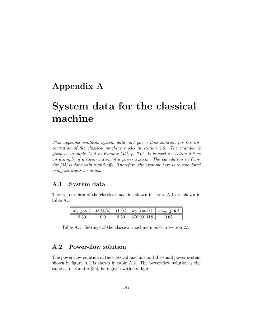
Appendix A

System data for the classicalmachine

This appendix contains system data and power-flow solution for the lin-earization of the classical machine model in section 2.5. The example isgiven as example 12.2 in Kundur [35], p. 732. It is used in section 2.5 asan example of a linearization of a power system. The calculation in Kun-dur [35] is done with round-offs. Therefore, the example here is re-calculatedusing six digits accuracy.

A.1 System data

The system data of the classical machine shown in figure A.1 are shown intable A.1.

x′d (p.u.) D (1/s) H (s) ω0 (rad/s) xline (p.u.)0.30 0.0 3.50 376.991118 0.65

Table A.1: Settings of the classical machine model in section 2.5.

A.2 Power-flow solution

The power-flow solution of the classical machine and the small power systemshown in figure A.1 is shown in table A.2. The power-flow solution is thesame as in Kundur [35], here given with six digits.

147

-

+

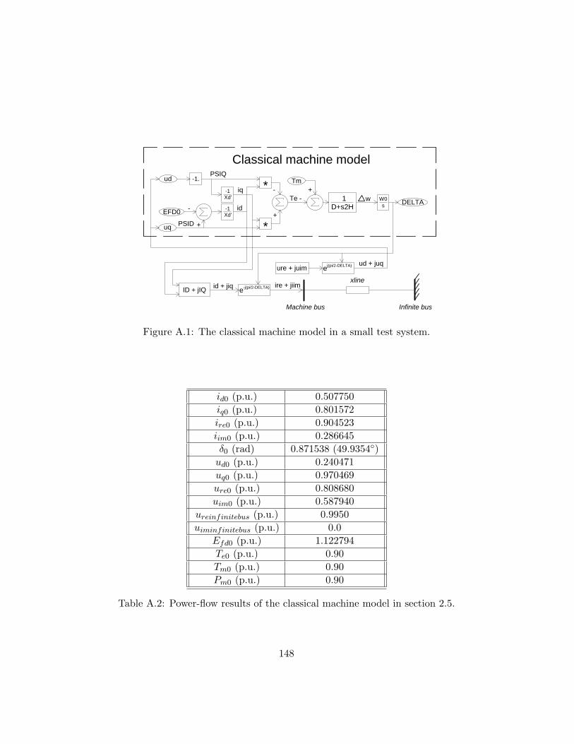
1D+s2H

DELTA

*

*

-1.

+- W0

s-

+

EFD0

-1Xd'

-1Xd'

ID + jIQ

Tmud

uq

e-j(pi/2-DELTA)

ej(pi/2-DELTA)ure + juim

iqTe

id

PSIQ

PSID

w

Classical machine model

xline

Infinite busMachine bus

id + jiq ire + jiim

ud + juq

Figure A.1: The classical machine model in a small test system.

id0 (p.u.) 0.507750iq0 (p.u.) 0.801572ire0 (p.u.) 0.904523iim0 (p.u.) 0.286645δ0 (rad) 0.871538 (49.9354)

ud0 (p.u.) 0.240471uq0 (p.u.) 0.970469ure0 (p.u.) 0.808680uim0 (p.u.) 0.587940

ureinfinitebus (p.u.) 0.9950uiminfinitebus (p.u.) 0.0

Efd0 (p.u.) 1.122794Te0 (p.u.) 0.90Tm0 (p.u.) 0.90Pm0 (p.u.) 0.90

Table A.2: Power-flow results of the classical machine model in section 2.5.

148

A.3 Linearization of example 12.2 in Kundur [35]

The power system shown in figure A.1 is used in section 2.5. Since thecalculation in Kundur [35] is done with round-offs, the result gets differentcompared to section 2.5 in this thesis even though the method is the same.Therefore, the example is here re-calculated using six digits accuracy. Below,the variable names are following Kundur [35].

The bus voltage at the machine bus, indicated as Et in Kundur [35] iswith six digits accuracy equal to,

Et = 0.9998186 36.0185 (A.1)

which is derived from the power-flow calculation.With Et as reference phasor, the generator stator current It in Kun-

dur [35] is,

It =(P + jQ)∗

E∗t

=0.9− j0.30.999818

=

= 0.900164− j0.300055(A.2)

The stator current It in Kundur [35] corresponds to ire + jiim in figureA.1 which is calculated with the infinite bus as reference phasor as,

ire + jiim = It · ej36.0185 = (0.900164− j0.300055) · ej36.0185 == 0.904523 + j0.286645

(A.3)

With the stator current It, the voltage behind the transient reactance,indicated as E′ in Kundur [35] can be calculated as,

E′ = Et + jX ′ · It = 0.999818 + j0.3 · (0.900164− j0.300055) == 1.089834 + j0.270049 = 1.122794 6 13.916961

(A.4)

The angle by which E′ leads EB (the rotor angle δ0) is,

δ0 = 13.916961 + 36.0185 = 49.935461 (A.5)

EB is the voltage for the infinite bus in Kundur [35]. The synchronizingtorque KS in Kundur [35] gets,

149

KS =E′ · EB

XTcos δ0 =

1.122794 · 0.9950.95

cos 49.935461 = 0.756919 (A.6)

The linear system that should be identified is,[∆ω

∆δ

]=

[A11 A12

A21 A22

] [∆ω∆δ

](A.7)

where the A-matrix is,

A =[

A11 A12

A21 A22

]. (A.8)

Matrix element A12 is equal to,

A12 = −KS

2H= −0.756919

2 · 3.5= −0.108131 (A.9)

The other matrix elements are the same in Kundur [35] as in section2.5.1.

The A-matrix gets,

A =[

0 −0.108131376.991118 0

](A.10)

which is the same as in section 2.5.1. The A-matrix gives the followingeigenvalues,

λ1,2 = 0± j6.38471(1/s, rad/s) (A.11)

which are the same as in section 2.5.1.

150

Appendix B

Truncation errors for theFDA and CDA methods

This appendix contains a detailed description of the truncation errors ob-tained when utilizing the FDA and CDA methods as described in chapter2.

B.1 Truncation error for the FDA method

When A12 was calculated in section 2.5.2 with equation (2.73) we includednon-linear feedback from the algebraic equations (2.37) – (2.45) to calculatethe value of the time-derivative of the speed deviation ∆ω when the machineangle δ had been disturbed with h from the equilibrium point.

When δ was disturbed, we calculated the feedback of the perturbationto the electrical torque Te in equation (2.67), below repeated as equation(B.1).

∆ω =1

2H(Tm − Te −D ·∆ω) (B.1)

Since the damping constant D is equal to zero in our example the lastterm D ·∆ω is deleted in equation (B.2).

∆ω =1

2H(Tm − Te) (B.2)

In the following we will rewrite equation (B.2) to derive ∆ω’s relationwith δ. If we re-write equation (2.37) we get,

Te = udid + uqiq. (B.3)

151

Equation (B.3) often can be seen containing the electrical power Pe (inp.u.) in the left-hand side. Since we here do not include any stator resistanceand that the rotor speed is ω = 1.0 we can write the electrical torque Te (inp.u.) in the left-hand side of equation (B.3), see Kundur [35], p. 175.

Instead of ud and uq we can apply equations (2.38) and (2.39) in equation(B.3). Then we get,

Te = ure(id sin δ + iq cos δ) + uim(iq sin δ − id cos δ). (B.4)

Instead of ure and uim we can apply equations (2.42) and (2.43) in equa-tion (B.4). Since uiminfinitebus = 0 we have excluded it in equation (B.5)below,

Te = (ureinfinitebus − xlineiim)(id sin δ + iq cos δ)++ xlineire(iq sin δ − id cos δ).

(B.5)

In equation (B.5) we can replace ire and iim with equations (2.44) and(2.45). With that, the equation for Te gets rather simplified and becomes,

Te = ureinfinitebus(iq cos δ + id sin δ). (B.6)

In equation (B.6) we then replace id and iq with the following two equa-tions,

id =Efd0 − ureinfinitebus · cos δ

x′d + xline

(B.7)

iq =ureinfinitebus · sin δ

x′d + xline

. (B.8)

Equation (B.7) has been derived by replacing uq in equation (2.40) withequation (2.39). Later ure and uim have been replaced with equations (2.42)and (2.43) respectively. Finally, the relation

id = ire sin δ − iim cos δ (B.9)

has been used. It can be identified from the block diagram with the expo-nential function e−j(π

2−δ) in the lower part of figure 2.2.

Equation (B.8) has been derived by replacing ud in equation (2.41) withequation (2.38). Later ure and uim have been replaced with equations (2.42)and (2.43) respectively. Finally, the relation

152

iq = ire cos δ + iim sin δ (B.10)

has been used. It can be identified from the block diagram with the expo-nential function e−j(π

2−δ) in the lower part of figure 2.2.

When we replace id and iq in equation (B.6) with equations (B.7) and(B.8) respectively we get,

Te =Efd0 · ureinfinitebus

x′d + xline

sin δ. (B.11)

Equation (B.11) shows Te’s relation with δ.As mentioned earlier, the electrical torque Te (in p.u.) in the left-hand

side of equation (B.11) can be replaced with electrical power Pe (in p.u.),see Kundur [35], p. 175.

The mechanical torque Tm is equal to the electrical torque Te since thetime-derivative of the speed deviation ∆ω of the machine is zero in theequilibrium point, see equation (B.2). Since Tm is constant for the classicalmachine it will therefore remain constantly equal to the value of equation(B.11) in the equilibrium point, i.e.,

Tm =Efd0 · ureinfinitebus

x′d + xline

sin δ0 (B.12)

during the perturbation of the machine angle δ,Now finally we can write an equation of how the speed deviation will

develop when we perturb the machine angle δ with h. We put equation(B.12) of Tm into equation (B.2). Te in equation (B.2) we replace withequation (B.11) with the perturbation h added to the machine angle δ. Weget,

∆ω =Efd0 · ureinfinitebus

2H · (x′d + xline)

(sin δ0 − sin(δ0 + h)) (B.13)

where δ0 is the machine angle in the equilibrium point.The matrix-element A12 is identified as with equation (2.73),

A12 =∆ω

∆δ(B.14)

where ∆ω is equal equation (B.13) and ∆δ is equal to the perturbation h.We get,

A12 =Efd0 · ureinfinitebus

2H · (x′d + xline) · h

(sin δ0 − sin(δ0 + h)). (B.15)

153

The expression sin(δ + h) we replace with,

sin(δ0 + h) = sin δ0 cos h + cos δ0 sinh (B.16)

and sinh and cos h can be Maclaurin developed as,

sinh = h− h3

6+

h5

120+ O(h7) (B.17)

cos h = 1− h2

2+

h4

24+ O(h6). (B.18)

Therefore equation (B.16) can be re-written as,

sin(δ0 + h) = sin δ0(1−h2

2+

h4

24) + cos δ0(h−

h3

6+

h5

120) + O(h6) (B.19)

If we put equation (B.19) in equation (B.15) and neglect orders higherthan O(h3) of the perturbation h we get the equation for A12FDA which wasearlier drawn as a function of h in figure 2.4,

A12FDA =Efd0 · ureinfinitebus

2H · (x′d + xline)

(− cos δ0+h

2sin δ0+

h2

6cos δ0)+O(h3) (B.20)

To obtain the truncation error ∆A12FDA, we have to subtract equation(B.20) with the analytical linearization of the same matrix element, i.e.,A12AL. The analytical linearization of equation (B.2) with respect to themachine angle δ is,

A12AL =∂

∂δ(∆ω) =

∂

∂δ(

12H

(Tm − Te)) =

=∂

∂δ(

12H

(Tm −Efd0 · ureinfinitebus · sin δ

x′d + xline

)) =

= − 12H

(Efd0 · ureinfinitebus · cos δ0

x′d + xline

)

(B.21)

In equation (B.21) we have replaced Te with the earlier derived equation(B.11).

The truncation error obtained with the FDA method, ∆A12FDA, is,

∆A12FDA = A12FDA −A12AL =

=Efd0 · ureinfinitebus

4H · (x′d + xline)

(h · sin δ0 +h2

3cos δ0) + O(h3)

(B.22)

154

B.2 Truncation error for the CDA method

In equation (B.13) we could see how the speed deviation develops when weperturb the machine angle δ with h. When using the CDA method we wanta similar expression when we perturb the load angle but with a negativeperturbation −h. Therefore we modify equation (B.13) to,

∆ωi− =Efd0 · ureinfinitebus

2H · (x′d + xline)

(sin δ0 − sin(δ0 − h)) (B.23)

where δ0 is the machine angle in the equilibrium point.The matrix-element A12 is when using the CDA method identified as

with equation (2.81),

A12 =∆ωi

∆δ=

∆ωi+ −∆ωi−2 ·∆δ

(B.24)

where ∆ωi+ is equal to ∆ω in equation (B.13), ∆ωi− is derived with equation(B.23), and ∆δ is equal to the perturbation h.

A12 can then be calculated as,

A12 =Efd0 · ureinfinitebus

2H · (x′d + xline)

(sin(δ0 − h)− sin(δ0 + h))2 · h

(B.25)

sin(δ0+h) in equation (B.25) is replaced with equation (B.19) and sin(δ0−h)is replaced with,

sin(δ0 − h) = sin δ0 cos h− cos δ0 sinh. (B.26)

Then equation (B.25) can be re-written as,

A12 = −Efd0 · ureinfinitebus · cos δ0 sinh

2H · (x′d + xline) · h

(B.27)

and sinh can be Maclaurin developed as in equation (B.17). If we neglectorders higher than 6 of the perturbation h we get the equation for A12CDA

which is drawn in figure 2.4,

A12CDA = −Efd0 · ureinfinitebus · cos δ0(1− h2

6 + h4

120 + O(h6))2H · (x′

d + xline)(B.28)

To obtain the truncation error ∆A12CDA, we have to subtract equation(B.28) with the analytical linearization of the same matrix element, i.e.,A12AL which also can be found in figure 2.4. A12AL was earlier derived

155

in equation (B.21). The truncation error obtained with the CDA method,∆A12CDA, is finally,

∆A12CDA = A12CDA −A12AL =

=Efd0 · ureinfinitebus

4H · (x′d + xline)

cos δ0 · (h2

3− h4

60) + O(h6).

(B.29)

By comparing equation (B.22) with equation (B.29) we can see that theterm h ·sin δ0 in equation (B.22) does not exist in equation (B.29). However,the term cos δ0 · h2

3 exist in both equations.

156

Appendix C

Implementation of the TCSC

This appendix contains a detailed description of the implemented originalTCSC model which has been the study object in the thesis when buildinglinear models.

C.1 Structure of the TCSC control

The series capacitor C and the series reactor L, sketched in figure C.1, aremodelled using the corresponding standard components in the used powersystem simulation software Simpow, see Fankhauser [16] and [75]. The restof the three-phase TCSC (the control algorithm and the thyristors) are splitup in three parts, one for each phase. Such a part has been implementedas a user-defined system in the software and each part has four underlyingfunctions which represent the control algorithm and the thyristors. Theseare,

• Phase Locked Loop (PLL)

• Booster (BOO)

• Thyristor Pulse Generator (TPG)

• Thyristors (THY)

which are shown in figure C.2 except for the function THY.The implementation of the TCSC follows the Synchronous Voltage Re-

versal control algorithm developed by ABB, see Angquist [88, 89]. Thecontrol system and its functionality are formulated by using the in-builtsimulation language Dynamic Simulation Language (DSL) in Simpow. One

157

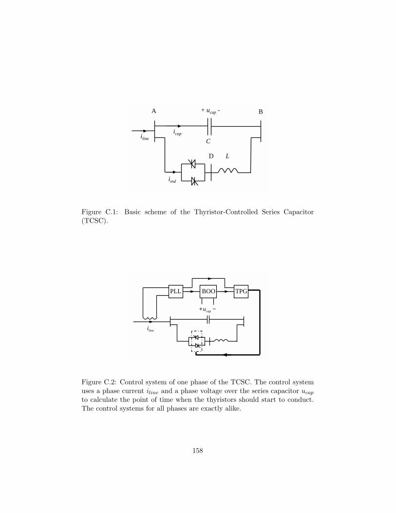
A + ucap - B

D L

C

iind

icapiline

Figure C.1: Basic scheme of the Thyristor-Controlled Series Capacitor(TCSC).

−+ capu

linei

PLL BOO TPG

Figure C.2: Control system of one phase of the TCSC. The control systemuses a phase current iline and a phase voltage over the series capacitor ucap

to calculate the point of time when the thyristors should start to conduct.The control systems for all phases are exactly alike.

158

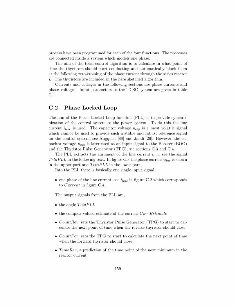
process have been programmed for each of the four functions. The processesare connected inside a system which models one phase.

The aim of the total control algorithm is to calculate in what point oftime the thyristors should start conducting and automatically block themat the following zero-crossing of the phase current through the series reactorL. The thyristors are included in the here sketched algorithm.

Currents and voltages in the following sections are phase currents andphase voltages. Input parameters to the TCSC system are given in tableC.1.

C.2 Phase Locked Loop

The aim of the Phase Locked Loop function (PLL) is to provide synchro-nization of the control system to the power system. To do this the linecurrent iline is used. The capacitor voltage ucap is a most volatile signalwhich cannot be used to provide such a stable and robust reference signalfor the control system, see Angquist [88] and Jalali [26]. However, the ca-pacitor voltage ucap is later used as an input signal to the Booster (BOO)and the Thyristor Pulse Generator (TPG), see sections C.3 and C.4.

The PLL extracts the argument of the line current iline, see the signalTetaPLL in the following text. In figure C.3 the phase current iline is shownin the upper part and TetaPLL in the lower part.

Into the PLL there is basically one single input signal,

• one phase of the line current, see iline in figure C.2 which correspondsto Current in figure C.4.

The output signals from the PLL are,

• the angle TetaPLL

• the complex-valued estimate of the current CurrEstimate

• CountRev, sets the Thyristor Pulse Generator (TPG) to start to cal-culate the next point of time when the reverse thyristor should close

• CountFor, sets the TPG to start to calculate the next point of timewhen the forward thyristor should close

• TimeRev, a prediction of the time point of the next minimum in thereactor current

159

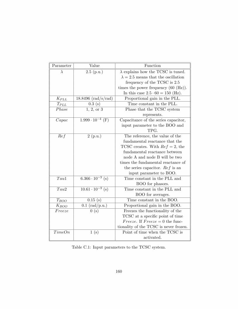
Parameter Value Functionλ 2.5 (p.u.) λ explains how the TCSC is tuned.

λ = 2.5 means that the oscillationfrequency of the TCSC is 2.5

times the power frequency (60 (Hz)).In this case 2.5 · 60 = 150 (Hz).

KPLL 18.8496 (rad/s/rad) Proportional gain in the PLL.TPLL 0.3 (s) Time constant in the PLL.Phase 1, 2, or 3 Phase that the TCSC system

represents.Capac 1.999 · 10−4 (F) Capacitance of the series capacitor,

input parameter to the BOO andTPG.

Ref 2 (p.u.) The reference, the value of thefundamental reactance that the

TCSC creates. With Ref = 2, thefundamental reactance betweennode A and node B will be two

times the fundamental reactance ofthe series capacitor. Ref is an

input parameter to BOO.Tau1 6.366 · 10−3 (s) Time constant in the PLL and

BOO for phasors.Tau2 10.61 · 10−3 (s) Time constant in the PLL and

BOO for averages.TBOO 0.15 (s) Time constant in the BOO.KBOO 0.1 (rad/p.u.) Proportional gain in the BOO.Freeze 0 (s) Freezes the functionality of the

TCSC at a specific point of timeFreeze. If Freeze = 0 the func-

tionality of the TCSC is never frozen.TimeOn 1 (s) Point of time when the TCSC is

activated.

Table C.1: Input parameters to the TCSC system.

160

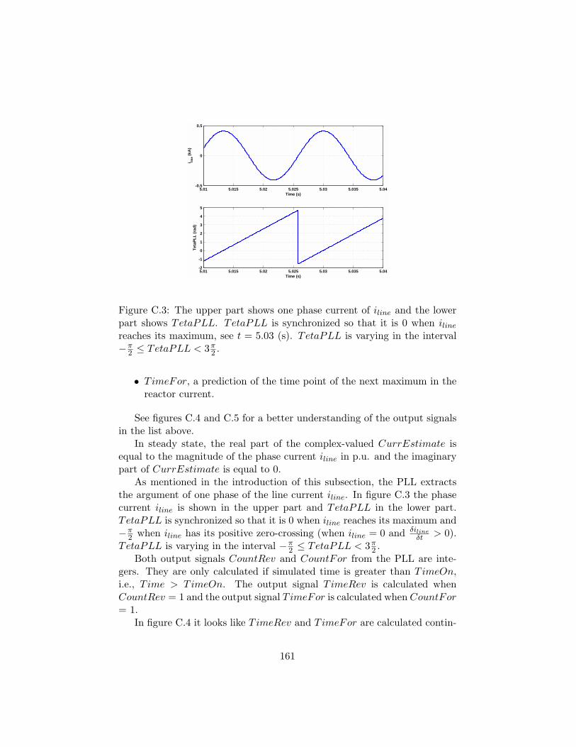
5.01 5.015 5.02 5.025 5.03 5.035 5.04-0.5

0

0.5

Time (s)i lin

e (kA

)

5.01 5.015 5.02 5.025 5.03 5.035 5.04-2

-1

0

1

2

3

4

5

Time (s)

Teta

PLL

(rad

)

Figure C.3: The upper part shows one phase current of iline and the lowerpart shows TetaPLL. TetaPLL is synchronized so that it is 0 when iline

reaches its maximum, see t = 5.03 (s). TetaPLL is varying in the interval−π

2 ≤ TetaPLL < 3π2 .

• TimeFor, a prediction of the time point of the next maximum in thereactor current.

See figures C.4 and C.5 for a better understanding of the output signalsin the list above.

In steady state, the real part of the complex-valued CurrEstimate isequal to the magnitude of the phase current iline in p.u. and the imaginarypart of CurrEstimate is equal to 0.

As mentioned in the introduction of this subsection, the PLL extractsthe argument of one phase of the line current iline. In figure C.3 the phasecurrent iline is shown in the upper part and TetaPLL in the lower part.TetaPLL is synchronized so that it is 0 when iline reaches its maximum and−π

2 when iline has its positive zero-crossing (when iline = 0 and δilineδt > 0).

TetaPLL is varying in the interval −π2 ≤ TetaPLL < 3π

2 .Both output signals CountRev and CountFor from the PLL are inte-

gers. They are only calculated if simulated time is greater than TimeOn,i.e., Time > TimeOn. The output signal TimeRev is calculated whenCountRev = 1 and the output signal TimeFor is calculated when CountFor= 1.

In figure C.4 it looks like TimeRev and TimeFor are calculated contin-

161

+

-

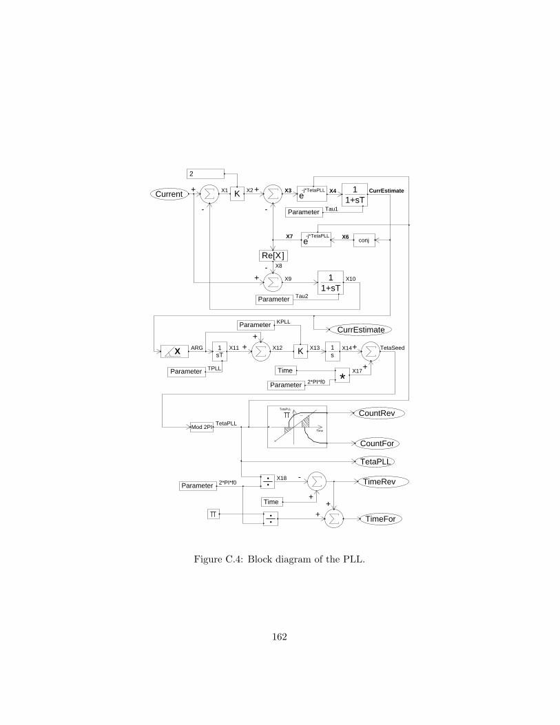
2

K +

-

11+sT

conj

X

]Re[X-

+ 11+sT

1sT K

Parameter

Mod 2PI

Parameter

Parameter

Parameter

Parameter

TetaPLL

+

+

1s

*

Current

CountRev

CountFor

Time

TetaPLL

Time

e-j*TetaPLL

e-j*TetaPLL

CurrEstimate

Parameter

Time

: -

+

TimeRev

:+

+ TimeFor

X1 X2 X3 X4 CurrEstimate

X6X7

X8

X9 X10

X13

TPLL

TetaSeed

TetaPLL

KPLL

2*PI*f0

Tau1

Tau2

X14

X17

2*PI*f0X18

++X11 X12ARG

Figure C.4: Block diagram of the PLL.

162

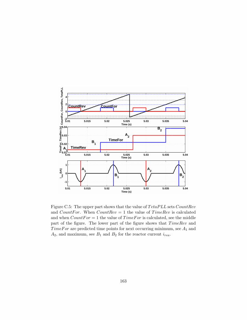
5.01 5.015 5.02 5.025 5.03 5.035 5.04-2

0

2

4

Time (s)Cou

ntFo

r, C

ount

Rev

, Tet

aPLL

5.01 5.015 5.02 5.025 5.03 5.035 5.045.01

5.02

5.03

5.04

Time (s)

Tim

eFor

, Tim

eRev

(s)

5.01 5.015 5.02 5.025 5.03 5.035 5.04

-1

0

1

Time (s)

i rea (k

A)

B1 B2 A1

A2

TimeRev

TimeFor

A1

A2

B1

B2

CountFor CountRev

Figure C.5: The upper part shows that the value of TetaPLL sets CountRevand CountFor. When CountRev = 1 the value of TimeRev is calculatedand when CountFor = 1 the value of TimeFor is calculated, see the middlepart of the figure. The lower part of the figure shows that TimeRev andTimeFor are predicted time points for next occurring minimum, see A1 andA2, and maximum, see B1 and B2 for the reactor current irea.

163

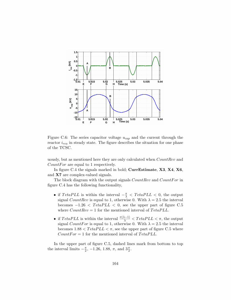
5.01 5.015 5.02 5.025 5.03 5.035 5.04-1.5

-1

-0.5

0

0.5

1

1.5

Time (s)

i rea (k

A)

5.01 5.015 5.02 5.025 5.03 5.035 5.04-15

-10

-5

0

5

10

15

Time (s)

u cap (k

V)

E F

E F

A

A

B

B

G H

HG

Figure C.6: The series capacitor voltage ucap and the current through thereactor irea in steady state. The figure describes the situation for one phaseof the TCSC.

uously, but as mentioned here they are only calculated when CountRev andCountFor are equal to 1 respectively.

In figure C.4 the signals marked in bold; CurrEstimate, X3, X4, X6,and X7 are complex-valued signals.

The block diagram with the output signals CountRev and CountFor infigure C.4 has the following functionality,

• if TetaPLL is within the interval −πλ < TetaPLL < 0, the output

signal CountRev is equal to 1, otherwise 0. With λ = 2.5 the intervalbecomes −1.26 < TetaPLL < 0, see the upper part of figure C.5where CountRev = 1 for the mentioned interval of TetaPLL.

• if TetaPLL is within the interval π(λ−1)λ < TetaPLL < π, the output

signal CountFor is equal to 1, otherwise 0. With λ = 2.5 the intervalbecomes 1.88 < TetaPLL < π, see the upper part of figure C.5 whereCountFor = 1 for the mentioned interval of TetaPLL.

In the upper part of figure C.5, dashed lines mark from bottom to topthe interval limits −π

2 , −1.26, 1.88, π, and 3π2 .

164

If CountRev = 1, then the prediction of next point of time A, see A1

and A2 in the lower part of figure C.5, is calculated with equation,

TimeRev = Time− TetaPLL

2πf0(C.1)

where Time is actual simulated time and f0 is the power frequency.If CountFor = 1, then the prediction of next point of time B, see B1

and B2 in the lower part of figure C.5, is calculated with equation,

TimeFor = Time +π − TetaPLL

2πf0. (C.2)

At points of time A and B, the reactor current irea is at its minimumand maximum respectively. At the same time the voltage drop ucap over thecapacitor has its zero crossings, see figure C.6.

The predictions of the time points TimeRev and TimeFor are laterimproved in the function BOO, see section C.3.

C.3 Booster

The Booster (BOO) has the following input signals,

• one phase of the series capacitor voltage, see ucap in figure C.2 whichcorresponds to V oltage in figure C.7

• the complex-valued current CurrEstimate

• the angle TetaPLL

• TimeRev, predicted time point from the PLL for the next positivezero-crossing in the series capacitor voltage ucap

• TimeFor, predicted time point from the PLL for the next negativezero-crossing in the series capacitor voltage ucap.

The last four input signals in the list above are calculated in the PLLfunction.

The output signals from the BOO are,

• TzRevNew, boosted points of time for the next positive zero-crossingin the series capacitor voltage ucap

165

+

-

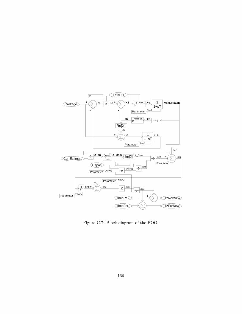
2

K +

-

11+sT

conj

]Re[X-

+ 11+sT

Parameter

Parameter

: :

:-1

1sT K

*Parameter

: -+

-+

Parameter

Ref+

-CurrEstimate SBASE

UBASE2

Voltage

TetaPLL

e-j*TetaPLL

e-j*TetaPLL

Parameter

Capac

TimeRev

TimeFor

TzRevNew

TzForNew

Im[X]

++

X1 X2 X3 X4 VoltEstimate

X6X7

X8

X9 X10

Tau1

Tau2

X_OhmZ_OhmZ_pu

PRODX21

X22 X23

X24

KBOO

X25 X26X27

TBOO

2*PI*f0

Boost factor

Figure C.7: Block diagram of the BOO.

166

• TzForNew, boosted points of time for the next negative zero-crossingin the series capacitor voltage ucap.

As mentioned above the results from the BOO are boosted points of timefor the next two zero-crossings of the series capacitor voltage, TzRevNewand TzForNew, see figure C.7. TzRevNew is the adjusted point of timeA and TzForNew is the adjusted point of time B in figure C.6. BOOis therefore boosting (improving) the predicted points of time TimeRev toTzRevNew and TimeFor to TzForNew from the function PLL, see sectionC.2. The BOO function is set to stand-by mode until Time ≥ TimeOn.When it is in stand-by mode, both TzRevNew and TzForNew are setequal to 0.

The functionality of the BOO can be frozen in a specific moment byspecifying a positive value (> 0) to the input parameter Freeze. If Freezeis specified to a positive value, the BOO function will at the same momentstop calculating new values of adjustments from the predictions of TimeRevand TimeFor which were calculated inside the PLL. In other words, whenTime > Freeze, the signal X27 in figure C.7 will be frozen to its currentvalue. If the input parameter Freeze is not specified then it is set to thedefault value 0 which means that the BOO function is active throughoutthe whole simulation.

In figure C.7 the signals marked in bold; CurrEstimate, VoltEstimate,X3, X4, X6, X7, Zpu, and ZOhm are complex-valued signals.

Since the phase voltage of the series capacitor voltage ucap is not perfectlysinusoidal, see the lower part of figure C.6, the real and imaginary part ofthe complex-valued V oltEstimate does not find constant values during asteady state wherein the TCSC is activated. However, the real part ofV oltEstimate is pending around 0 and the imaginary part of V oltEstimateis pending around a negative value of the magnitude of the series capacitorvoltage ucap. This since the voltage drop over a capacitor is 90 behind itscurrent. The steady-state current is estimated in the PLL and is in steadystate of pure real character as was mentioned earlier in section C.2.

C.4 Thyristor Pulse Generator

The aim of the Thyristor Pulse Generator (TPG) is to calculate the pointsof time when the thyristors should start conducting. Pulse signals are thengenerated to fire each thyristor (FireRev and FireFor). The pulse signalsare set when the forward and the reverse thyristor should start to conduct

167

respectively. As long as (Time < TimeOn), the TPG is in stand-by modeand FireRev and FireFor are both set equal to 0.

The equations of the TPG are shown in figure C.8 but can also be foundin Angquist [88], pp. 51-54.

The TPG has the following input signals,

• TzRevNew, boosted points of time from the BOO for the next positivezero-crossing in the series capacitor voltage ucap

• TzForNew, boosted points of time from the BOO for the next nega-tive zero-crossing in the series capacitor voltage ucap

• one phase of the series capacitor voltage ucap referred to as V oltage infigure C.8

• one phase of the line current iline referred to as Current in figure C.8

• BlowRev, order from the function Thyristors (THY) to open the re-verse thyristor

• BlowFor, order from the function THY to open the reverse thyristor.

The last two input signals in the list above are not viewed in figure C.8of the TPG.

The output signals from the TPG are,

• FireRev, command to the reverse thyristor to start to conduct

• FireFor, command to the forward thyristor to start to conduct.

When the calculated conducting time TfRev or TfFor in figure C.8 areequal to actual simulated time, the output signals FireRev and FireForare set equal to 1 respectively. These output signals are input signals to thefunction THY and they are commands to the thyristors to start conducting.Once a thyristor has start to conduct it conducts until the following zero-crossing of the current.

FireRev and FireFor are equal to 1 as long as the corresponding thyris-tor is conducting and remain equal to 1 until they are reset by the signalsBlowRev and BlowFor which are generated in the function THY. WhenBlowRev or BlowFor are equal to 1, FireRev or FireFor are set equal to0 and the corresponding thyristors are then blocked in the function THY.

168

*

+

-

:

*+

+

-+ *

++

*

:

:+

-

+-

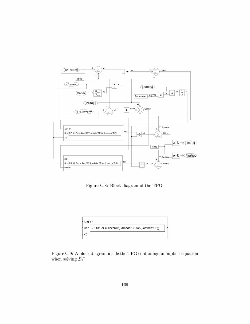
a=b

a=b

FireFor

Time

Time

FireRev

TzForNew

Current

Capac SBASE

UBASE2

Voltage

TzRevNew

Parameter

Lambda1x

Y1

Y2

Y3Y4

Y5Y8

Y6Y7

Y10

Y9 TfFor

TfRev

2*PI*f0

TzForNew

TzRevNew

BF: UzFor = iline*X0*(Lambda*BF-tan(Lambda*BF))

UzFor

iline

X0

UzFor

BF

BR: UzRev = iline*X0*(Lambda*BR-tan(Lambda*BR))

UzRev

iline

X0

X0

UzRev

BR

Figure C.8: Block diagram of the TPG.

BF: UzFor = iline*X0*(Lambda*BF-tan(Lambda*BF))

UzFor

iline

X0

Figure C.9: A block diagram inside the TPG containing an implicit equationwhen solving BF .

169

Phase ThyristorA ForwardC ReverseB ForwardA ReverseC ForwardB Reverse

Table C.2: The order of the thyristor switches.

The block diagram showed in figure C.9 is an enlargement of the blockdiagram in figure C.8 which solves the forward variable BF with the implicitequation,

UzFor = iline ·X0 · (λ ·BF − tan(λ ·BF )). (C.3)

The output signal from the block diagram in figure C.9 is BF .A similar block diagram is used for the reverse variable BR in figure C.8.

C.5 Thyristors

Into the function Thyristors (THY) the signals FireRev and FireFor areinput signals which are generated in the TPG. These signals command thethyristors to start to conduct. The thyristors are conducting until the fol-lowing zero-crossing of the current through the thyristors. When the currentthrough the thyristor reaches zero the signals BlowRev and BlowFor re-spectively are set equal to 1. BlowRev and BlowFor are sent to the TPGand when they are equal to 1, FireRev and FireFor respectively are resetin the TPG and as a consequence, the thyristors are opened.

C.6 The rhythm of the thyristors

The thyristors turn on within one period in the order as given in table C.2.Every thyristor is automatically turned off when the current through it hasits zero crossing, see the upper part of figure C.6.

170

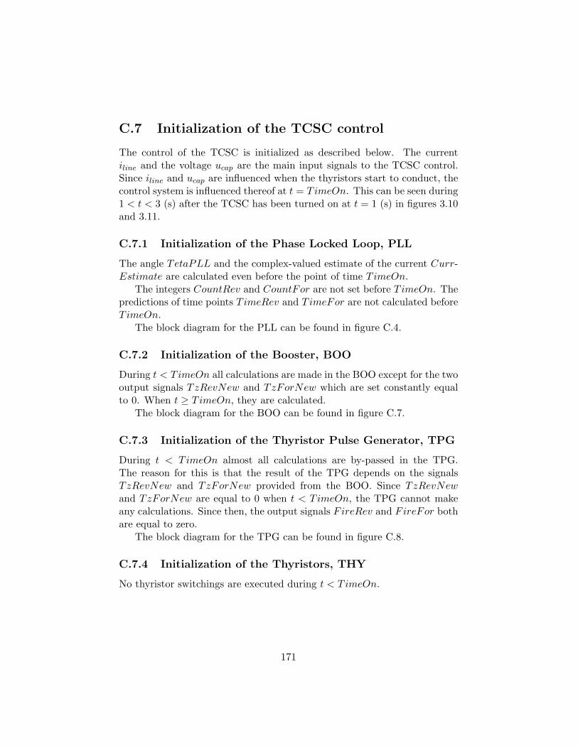
C.7 Initialization of the TCSC control

The control of the TCSC is initialized as described below. The currentiline and the voltage ucap are the main input signals to the TCSC control.Since iline and ucap are influenced when the thyristors start to conduct, thecontrol system is influenced thereof at t = TimeOn. This can be seen during1 < t < 3 (s) after the TCSC has been turned on at t = 1 (s) in figures 3.10and 3.11.

C.7.1 Initialization of the Phase Locked Loop, PLL

The angle TetaPLL and the complex-valued estimate of the current Curr-Estimate are calculated even before the point of time TimeOn.

The integers CountRev and CountFor are not set before TimeOn. Thepredictions of time points TimeRev and TimeFor are not calculated beforeTimeOn.

The block diagram for the PLL can be found in figure C.4.

C.7.2 Initialization of the Booster, BOO

During t < T imeOn all calculations are made in the BOO except for the twooutput signals TzRevNew and TzForNew which are set constantly equalto 0. When t ≥ TimeOn, they are calculated.

The block diagram for the BOO can be found in figure C.7.

C.7.3 Initialization of the Thyristor Pulse Generator, TPG

During t < T imeOn almost all calculations are by-passed in the TPG.The reason for this is that the result of the TPG depends on the signalsTzRevNew and TzForNew provided from the BOO. Since TzRevNewand TzForNew are equal to 0 when t < T imeOn, the TPG cannot makeany calculations. Since then, the output signals FireRev and FireFor bothare equal to zero.

The block diagram for the TPG can be found in figure C.8.

C.7.4 Initialization of the Thyristors, THY

No thyristor switchings are executed during t < T imeOn.

171

172

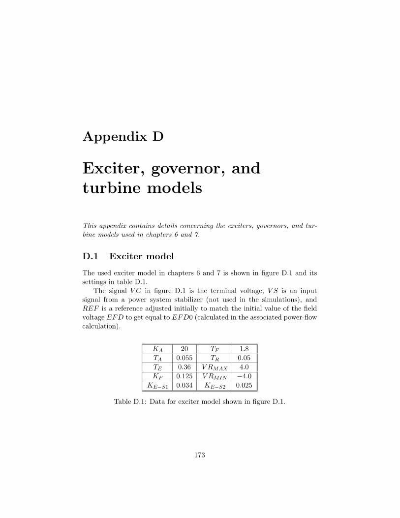
Appendix D

Exciter, governor, andturbine models

This appendix contains details concerning the exciters, governors, and tur-bine models used in chapters 6 and 7.

D.1 Exciter model

The used exciter model in chapters 6 and 7 is shown in figure D.1 and itssettings in table D.1.

The signal V C in figure D.1 is the terminal voltage, V S is an inputsignal from a power system stabilizer (not used in the simulations), andREF is a reference adjusted initially to match the initial value of the fieldvoltage EFD to get equal to EFD0 (calculated in the associated power-flowcalculation).

KA 20 TF 1.8TA 0.055 TR 0.05TE 0.36 V RMAX 4.0KF 0.125 V RMIN −4.0

KE−S1 0.034 KE−S2 0.025

Table D.1: Data for exciter model shown in figure D.1.

173

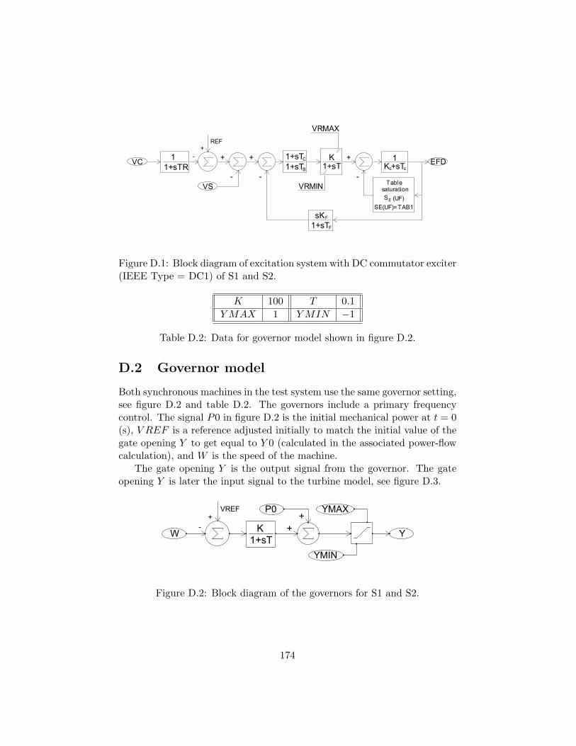
11+sTRVC

REF+

- +

-VS

+

-

1+sTsKF

F

1+sTB

C

1+sTK

1+sT+

-saturationSE (UF)

Table

SE(UF)=TAB1

1+sTK EE

VRMAX

VRMIN

EFD

Figure D.1: Block diagram of excitation system with DC commutator exciter(IEEE Type = DC1) of S1 and S2.

K 100 T 0.1Y MAX 1 Y MIN −1

Table D.2: Data for governor model shown in figure D.2.

D.2 Governor model

Both synchronous machines in the test system use the same governor setting,see figure D.2 and table D.2. The governors include a primary frequencycontrol. The signal P0 in figure D.2 is the initial mechanical power at t = 0(s), V REF is a reference adjusted initially to match the initial value of thegate opening Y to get equal to Y 0 (calculated in the associated power-flowcalculation), and W is the speed of the machine.

The gate opening Y is the output signal from the governor. The gateopening Y is later the input signal to the turbine model, see figure D.3.

K1+sT

++ YW

P0 YMAX

YMIN

VREF+

-

Figure D.2: Block diagram of the governors for S1 and S2.

174

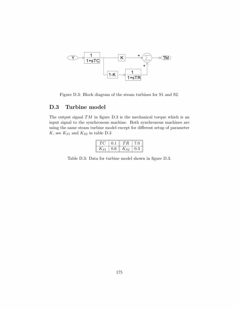
Y +

+

TMK

1-K

11+sTC

11+sTR

Figure D.3: Block diagram of the steam turbines for S1 and S2.

D.3 Turbine model

The output signal TM in figure D.3 is the mechanical torque which is aninput signal to the synchronous machine. Both synchronous machines areusing the same steam turbine model except for different setup of parameterK, see KS1 and KS2 in table D.3

TC 0.1 TR 7.0KS1 0.6 KS2 0.3

Table D.3: Data for turbine model shown in figure D.3.

175

176

Bibliography

[1] Goran Andersson, Discussions with Goran Andersson, 1998 – 2005.

[2] Goran Andersson, Modelling and Analysis of Electric Power Systems,EEH - Power Systems Laboratory, ETH, Zurich, Switzerland, March,2004.

[3] Kjell Aneros, Discussions with Kjell Aneros, 1998 – 2005.

[4] Kjell Aneros, Simpow: Methods and DSL-extensions for Dynpow simu-lations, STRI AB, Ludvika, Sweden, September 1, 2004.

[5] H. Buhler, Einfuhrung in die Theorie geregelter Drehstromantriebe -Band 1: Grundlagen, Birkhauser, 1977.

[6] I.M. Canay, Advance calculation of the characteristic quantities of syn-chronous machines and comparison with measured values, IEE Proceed-ings, Vol. 141, No. 1, 1994.

[7] N. Christl, R. Hedin, R. Johnson, P. Krause, A. Montoya, Power systemstudies and modelling for the Kayenta 230 kV substation advanced se-ries compensation, in Proceedings of the 5th IEE International Confer-ence on AC and DC Power Transmission 1991, London, Great Britain,September 17th – 20th, 1991, pp. 33–37.

[8] N. Christl, R. Hedin, K. Sadek, P. Lutzelberger, P.E. Krause,S.M. McKenna, A.H. Montoya, D. Torgerson, Advanced Series Compen-sation (ASC) with Thyristor Controlled Impedance, CIGRE 14/37/38-05, August 1992.

[9] Ian Dobson, Emilio Barocio, Perturbations of Weakly Resonant PowerSystem Electromechanical Modes, IEEE Transactions on Power Sys-tems, Vol. 20, No. 1, February 2005, pp. 330–337.

177

[10] Ian Dobson, Stability of Ideal Thyristor and Diode Switching Circuits,IEEE Transactions on Circuit and Systems–I: Fundamental Theory andApplications, Vol. 42, No. 9, September 1995, pp. 517–529.

[11] Ian Dobson, Stability and nonlinear dynamics in thyristor and diodecircuits, preprint March 22, 2001 of chapter 6 in Nonlinear Phenomenain Power Electronics: Attractors, Bifurcations, Chaos, and NonlinearControl, Editors S. Banerjee, G.C. Verghese, IEEE Press, to appear inSpring 2001.

[12] W.A. Docter, C. Georgakis, Identification of Reduced Order AverageLinear Models from Nonlinear Dynamic Simulations, in Proceedingsof the American Control Conference 1997, Vol. 5, Albuquerque, NewMexico, USA, June 4th – 6th, 1997, pp. 3047–3052.

[13] P.S. Dolan, J.R. Smith, W.A. Mittelstadt, Prony Analysis and Model-ing of a TCSC Under Modulation Control, in Proceedings of the 4thIEEE Conference on Control Applications, September 28th – 29th,1995, pp. 239–245.

[14] Olle I. Elgerd, Electric Energy Systems Theory – An Introduction, 2ndEdition, McGraw-Hill, 1982.

[15] G. Escobar, A.M. Stankovic, P. Mattavelli, R. Ortega, A comparativestudy of three nonlinear controllers for TCSC, in Proceedings of theIEEE Porto Power Tech Conference 2001, PPT’01, paper 368, Porto,Portugal, September 10th – 13th, 2001.

[16] Hans Fankhauser, Ture Adielson, Kjell Aneros, Abdel-Aty Edris, LarsLindkvist, Sture Torseng, Simpow – a digital power system simulator,Reprint of ABB Review, No. 7, 1990.

[17] A. Ghosh, G. Ledwich, Modelling and control of thyristor-controlled se-ries compensators, IEE Proc.-Gener. Transm. Distrib., Vol. 142, No. 3,May, 1995.

[18] Philip E. Gill, Walter Murray, Margaret H. Wright, Practical Optimiza-tion, Academic Press, 1981.

[19] Torkel Glad, Lennart Ljung, Reglerteori – Flervariabla och olinjarametoder, Studentlitteratur, 1997, in Swedish.

[20] Narain G. Hingorani, Laszlo Gyugyi, Understanding FACTS, the IEEEPress Marketing, 2000.

178

[21] IEEE Brown Book, IEEE Recommended Practice for Industrial andCommercial Power Systems Analysis, IEEE Std 399-1990, 1990.

[22] Gunnar Ingestrom, Simpow model of a TCSC, TR POW/RS 94–016,ABB Power Systems, Vasteras, Sweden, August 19, 1994.

[23] Sasan G. Jalali, Harmonics and Instabilities in Thyristor Based Switch-ing Circuits, Ph.D. thesis, University of Wisconsin at Madison, USA,1993.

[24] Sasan G. Jalali, Ian Dobson, Robert H. Lasseter, Giri Venkataramanan,Switching Time Bifurcations in a Thyristor Controlled Reactor, IEEETransactions on Circuit and Systems–I: Fundamental Theory and Ap-plications, Vol. 43, No. 3, March 1996, pp. 209–218.

[25] Sasan G. Jalali, Ron A. Hedin, Marcos Pereira, Kadry Sadek, A Stabil-ity Model for the Advanced Series Compensator (ASC), IEEE Transac-tions on Power Delivery, Vol. 11, No. 2, April 1996, pp. 1128–1137.

[26] Sasan G. Jalali, Robert H. Lasseter, Ian Dobson, Dynamic Responseof a Thyristor Controlled Switched Capacitor, IEEE Transactions onPower Delivery, Vol. 9, No. 3, July 1994, pp. 1609–1615.

[27] Emil Johansson, Detailed description of Synchronous Machine Mod-els used in Simpow, Technical Report TR H 01–160, ABB Utilities,Vasteras, Sweden, December 18, 2001.

[28] Emil Johansson, Jonas Persson, Lars Lindkvist, Lennart Soder, Lo-cation of Eigenvalues Influenced by Different Models of SynchronousMachines, in Proceedings of the 6th IASTED International Multi–Conference on Power and Energy Systems, Paper 352–145, Marina delRey, Los Angeles, USA, May 13th – 15th, 2002.

[29] Dragan Jovcic, G.N. Pillai, Analytical Modeling of TCSC Dynamics,IEEE Transactions on Power Delivery, Vol. 20, No. 2, April 2005,pp. 1097–1104.

[30] K.K. Kaberere, K.A. Folly, M. Ntombela, A.I. Petroianu, ComparativeAnalysis and Numerical Validation of Industrial-grade Power SystemSimulation Tools: Application to Small-signal Stability, in Proceedingsof the 15th Power Systems Computation Conference 2005, PSCC’05,Paper 26–3, Liege, Belgium, August 22nd – 26th, 2005.

179

[31] Keren Kaberere, Mpumelelo Ntombela, Komla Folly, AlexanderPetroianu, Comparison of Industrial-Grade Analytical Tools Used inSmall-Signal Stability Assessment, Internal Report, University of CapeTown, Dept. of Electrical Engineering, Rondebosch, Cape Town, SouthAfrica, 2005.

[32] Steven M. Kay, Fundamentals of Statistical Signal Processing: Estima-tion Theory, Prentice-Hall Inc., 1993.

[33] Hans Knudsen, chapter 24 in Thomas Ackermann, Wind Power inPower Systems, John Wiley & Sons Ltd., 2005.

[34] P.K. Kovacs, Studies in Electrical and Electronic Engineering 9, Tran-sient Phenomena in Electrical Machines, Elsevier, 1984.

[35] Prabha Kundur, Power System Stability and Control, The EPRI PowerSystem Engineering Series, McGraw-Hill, 1994.

[36] Prabha Kundur, John Paserba, Venkat Ajjarapu, Goran Andersson,Anjan Bose, Claudio Canizares, Nikos Hatziargyriou, David Hill, AlexStankovic, Carson Taylor, Thierry Van Cutsem, Vijay Vittal, Definitionand Classification of Power System Stability, IEEE/CIGRE Joint TaskForce on Stability Terms and Definitions, IEEE Transactions on PowerSystems, Vol. 19, No. 2, May 2004, pp. 1387–1401.

[37] Prabha Kundur, John Paserba, Sylvain Vitet, Overview on Defi-nition and Classification of Power System Stability, On behalf ofIEEE/CIGRE Joint Task Force on Stability Terms and Definitions.Quality and Security of Electric Power Delivery Systems, 2003,CIGRE/IEEE PES International Symposium, October 8th – 10th,2003.

[38] Th. Laible, Die Theorie der Synchronmaschine im nichtstationaren Be-trieb, Springer, 1952.

[39] Bengt Lennartson, Bertil Thomas, Analog och digital reglerteknik –ovningsbok, Studentlitteratur, 1988, in Swedish.

[40] Lennart Ljung, System Identification, Theory For The User, Prentice-Hall Inc., 1999.

[41] Lennart Ljung, System Identification Toolbox, For Use with Matlab –User’s Guide, The Mathworks Inc., June, 1994.

180

[42] Jan Machowski, Janusz W. Bialek, James R. Bumby, Power SystemDynamics and Stability, John Wiley & Sons Ltd., 1997.

[43] Nelson Martins, Efficient Eigenvalue and Frequency Response MethodsApplied to Power System Small-Signal Stability Studies, IEEE Trans-actions on Power Systems, Vol. PWRS-1, February 1986, pp. 217–226.

[44] Nelson Martins, Leonardo T.G. Lima, Determination of Suitable Lo-cations for Power System Stabilizers and Static Var Compensators forDamping Electromechanical Oscillations in Large Scale Power Systems,IEEE Transactions on Power Systems, Vol. 5, No. 4, November 1990,pp. 1455–1469.

[45] Paolo Mattavelli, Aleksandar M. Stankovic, George C. Verghese, SSRAnalysis with Dynamic Phasor Model of Thyristor-Controlled SeriesCapacitor, IEEE Transactions on Power Systems, Vol. 14, No. 1, Febru-ary 1999.

[46] Paolo Mattavelli, George C. Verghese, Aleksandar M. Stankovic, Pha-sor Dynamics of Thyristor-Controlled Series Capacitor Systems, IEEETransactions on Power Systems, Vol. 12, No. 3, August 1997, pp. 1259–1267.

[47] Hans-Peter Nee, Mats Leksell, Lennart Soder, Stefan Ostlund, Eleffek-tsystem, Literature to the course Electric Power Systems, Departmentof Electrical Engineering, Electric Power Systems, Royal Institute ofTechnology, Stockholm, Sweden, October, 2003, in Swedish.

[48] Hisham A. Othman, Lennart Angquist, Analytical Modeling ofThyristor-Controlled Series Capacitors for SSR studies, IEEE Trans-actions on Power Systems, Vol. 11, No. 1, February 1996, pp. 119–127.

[49] R.H. Park, Two-Reaction Theory of Synchronous Machines – General-ized Method of Analysis – Part I, A.I.E.E. Transactions, Vol. 48, July,1929, pp. 716–727; Part II, Vol. 52, June, 1933, pp. 352–355.

[50] J. Paserba (ed.), Analysis and Control of Power System Oscillations,Paris: CIGRE technical brochure, July, 1996.

[51] Jonas Persson, A description of the Masta model of the Thyristor-Controlled Series Capacitor in Simpow, Technical Report, TR H 00–163A, ABB Power Systems, Vasteras, Sweden, October 12, 2000.

181

[52] Jonas Persson, Are there any Limits in Building Small-Signal Modelsof Dynamic Systems?, Internal Report, Department of Electric PowerEngineering, Electric Power Systems, Royal Institute of Technology,Stockholm, Sweden, 1999.

[53] Jonas Persson, Help manual for the Fast Fourier Transform-Algorithmin Simpow, Technical Report, TR POW/H 51–106A, ABB Power Sys-tems, Vasteras, Sweden, August 24, 1998.

[54] Jonas Persson, How linearization is made in a small power system witha classical representation of a synchronous machine, Internal Report,Department of Electrical Engineering, Electric Power Systems, RoyalInstitute of Technology, Stockholm, Sweden, 2002.

[55] Jonas Persson, Linear Models of Non-linear Power System Components,Licentiate Thesis, TRITA-ETS-2001-04, ISSN 1650-674X, Departmentof Electrical Engineering, Electric Power Systems, Royal Institute ofTechnology, Stockholm, Sweden, 2002.

[56] Jonas Persson, On Linearization of Non-linear Components, A-EES-0014, Internal Report, Department of Electric Power Engineering, Elec-tric Power Systems, Royal Institute of Technology, Stockholm, Sweden,2000.

[57] Jonas Persson, Kjell Aneros, Jean-Philippe Hasler, Switching a LargePower System Between Fundamental Frequency and InstantaneousValue Mode, in Proceedings of the 3rd International Conference on Dig-ital Power System Simulators, ICDS’99, Vasteras, Sweden, May 25th– 28th, 1999.

[58] Jonas Persson, Luis Rouco, Lennart Soder, Linear Analysis with TwoLinear Models of a Thyristor-Controlled Series Capacitor, in Proceed-ings of the IEEE Bologna Power Tech Conference 2003, BPT’03, Paper496, Bologna, Italy, June 23rd – 26th, 2003.

[59] Jonas Persson, Luis Rouco, Lennart Soder, Time-Domain Comparisonsof Two Linear Models of a Thyristor-Controlled Series Capacitor, inProceedings of the 6th International Power Engineering Conference,IPEC’03, Paper 1046, Singapore, November 27th – 29th, 2003.

[60] Jonas Persson, Han Slootweg, Luis Rouco, Lennart Soder, Wil Kling,A Comparison of Eigenvalues Obtained with Two Dynamic SimulationSoftware Packages, in Proceedings of the IEEE Bologna Power Tech

182

Conference 2003, BPT’03, Paper 254, Bologna, Italy, June 23rd – 26th,2003.

[61] Jonas Persson, Lennart Soder, Linear Analysis of a Two-Area SystemIncluding a Linear Model of a Thyristor-Controlled Series Capacitor, inProceedings of the IEEE Porto Power Tech Conference 2001, PPT’01,Paper 289, Porto, Portugal, September 10th – 13th, 2001.

[62] Jonas Persson, Lennart Soder, Validity of a Linear Model of aThyristor-Controlled Series Capacitor for Dynamic Simulations, inProceedings of the 14th Power Systems Computation Conference 2002,PSCC’02, Paper 26–6, Sevilla, Spain, June 24th – 28th, 2002.

[63] G. Peters, J.H. Wilkinson, Inverse Iteration, Ill-Conditioned Equationsand Newton’s Method, SIAM Review, Vol. 21, No. 3, July, 1979.

[64] Jan Petersson, Fourieranalys, Jan Petersson, Dalmans vag 9, 434 97Kungsbacka, Sweden, in Swedish.

[65] John G. Proakis, Dimitris G. Manolakis, Digital Signal Processing –Principles, Algorithms, and Applications, Macmillan Publishing Com-pany, 1992.

[66] Manitoba HVDC Research Centre Inc. homepage,http://www.pscad.com.

[67] PSS/E, Online Documentation, Schenectady, Power Technologies, Inc.,December, 1997.

[68] PSS/E, Program Application Guide: Volume II, Online Documentation,PSS/E–29, Power Technologies, Inc., October, 2002.

[69] Rajesh Rajaraman, Ian Dobson, Justification of torque per unit velocitymethods of analyzing subsynchronous resonance and a swing mode inpower systems, IEEE Transactions on Circuits and Systems I: Fun-damental Theory and Applications, Vol. 45, No. 10, October 1998,pp. 1109–1113.

[70] Rajesh Rajaraman, Ian Dobson, Sasan G. Jalali, Nonlinear Dynam-ics and Switching Time Bifurcations of a Thyristor Controlled ReactorCircuit, IEEE Transactions on Circuits and Systems I: FundamentalTheory and Applications, Vol. 43, No. 12, December 1996, pp. 1001–1006.

183

[71] Rajesh Rajaraman, Ian Dobson, Robert H. Lasseter, Yihchih Stern,Computing the Damping of Subsynchronous Oscillations due to aThyristor Controlled Series Capacitor, IEEE Transactions on PowerDelivery, Vol. 11, No. 2, April 1996, pp. 1120–1127.

[72] Rajesh Rajaraman, Ian Dobson, Damping and incremental energy inthyristor switching circuits, in Proceedings of IEEE International Sym-posium on Circuits and Systems, Seattle, USA, May, 1995, pp. 291–294.

[73] J.J. Sanchez-Gasca, K. Clark, N.W. Miller, H. Okamoto, A. Kurita,J.H. Chow, Identifying Linear Models from Time Domain Simulations,IEEE Computer Applications in Power, Vol. 10, No. 2, April 1997,pp. 26–30.

[74] Bengt Schmidtbauer, Analog och digital reglerteknik, Studentlitteratur,1988, in Swedish.

[75] The reference manual of Simpow, STRI AB, Ludvika, Sweden, March29, 2004.

[76] Sigurd Skogestad, Discussions with Sigurd Skogestad, 2004 – 2005.

[77] Sigurd Skogestad, Ian Postlethwaite, Multivariable Feedback Control –Analysis and Design, John Wiley & Sons Ltd., 1996.

[78] J.G. Slootweg, Jonas Persson, A.M. van Voorden, G.C. Paap, WilKling, A Study of the Eigenvalue Analysis Capabilities of Power Sys-tem Dynamics Simulation Software, in Proceedings of the 14th PowerSystems Computation Conference 2002, PSCC’02, Paper 26–3, Sevilla,Spain, June 24th – 28th, 2002.

[79] Thomas Smed, Interaction Between High Voltage ac and dc systems,Ph.D. thesis, Dept. Electric Power Engineering, Royal Institute of Tech-nology, Stockholm, Sweden, 1991.

[80] A.M. Stankovic, P. Mattavelli, V. Caliskan, G.C. Verghese, Modelingand Analysis of FACTS Devices with Dynamic Phasors, IEEE PowerEngineering Society Winter Meeting 2000, Singapore, Vol. 2, January23rd – 27th, 2000.

[81] J.H. Taylor, A.J. Antoniotti, Linearization algorithms and heuristicsfor computer-aided control engineering, in Proceedings of Computer-Aided Control System Design 1992 (CACSD), 1992 IEEE Symposium,March 17th – 19th, 1992, pp. 156–164.

184

[82] J.H. Taylor, A.J. Antoniotti, Linearization algorithms for computer-aided control engineering, IEEE Control Systems Magazine, Vol. 13,Issue 2, April, 1993, pp. 58–64.

[83] Heinz Unbehauen, Ganti Prasada Rao, Identification of ContinuousSystems, North-Holland Systems and Control Series, Vol. 10, 1987.

[84] U.S.–Canada Power System Outage Task Force, Final Report on theAugust 14, 2003 Blackout in the United States and Canada: Causesand Recommendations, April, 2004, U.S. Department of Energy, Wash-ington, DC, USA, available at https://reports.energy.gov/.

[85] David S. Watkins, Understanding the QR Algorithm, SIAM Review,Vol. 24, No. 4, October, 1982.

[86] J.H. Wilkinson, The Algebraic Eigenvalue Problem, Numerical Mathe-matics and Scientific Computation, Oxford Science Publications, Ox-ford University Press, 1965.

[87] Lennart Angquist, Discussions with Lennart Angquist, 1998 – 2006.

[88] Lennart Angquist, Synchronous Voltage Reversal Control of ThyristorControlled Series Capacitor, Ph.D. thesis, Dept. Electrical Engineering,Royal Institute of Technology, Stockholm, Sweden, 2002.

[89] Lennart Angquist, Gunnar Ingestrom, Hans-Ake Jonsson, DynamicalPerformance of TCSC Schemes, CIGRE Session – 1996, Paper 14–302.

185