BANCO DE PORTUGAL

Economic Research Department

UNIQUE EQUILIBRIUM WITH SINGLE MONETARY

INSTRUMENT RULES

Bernardino Adão

Isabel Correia

Pedro Teles

WP 12-05 November 2005

The analyses, opinions and findings of these papers represent the views of the

authors, they are not necessarily those of the Banco de Portugal.

Please address correspondence to Banco de Portugal, Economic Research Department,

Av. Almirante Reis, no. 71 1150–012 Lisboa, Portugal;

Bernardino Adão, tel: # 351-21-3128409, email: badao@bportugal.pt;

Isabel Correia, tel: # 351-21-3128385, email: mihcarvalho@bportugal.pt;

Pedro Teles, tel: # 351-21-3130035, email: pmpteles@bportugal.pt.

Unique Equilibrium with Single MonetaryInstrument Rules.�

Bernardino AdãoBanco de Portugal

Isabel CorreiaBanco de Portugal, Universidade Catolica Portuguesa and CEPR

Pedro TelesBanco de Portugal, Universidade Catolica Portuguesa,

Federal Reserve Bank of Chicago, CEPR.

November, 2005

AbstractWe consider standard cash-in-advance monetary models and show that

there are interest rate or money supply rules such that equilibria are unique.The existence of these single instrument rules depends on whether the econ-omy has an in�nite horizon or an arbitrarily large but �nite horizon.Key words: Monetary policy; interest rate rules; unique equilibrium.JEL classi�cation: E31; E40; E52; E58; E62; E63.

1. Introduction

In this paper we revisit the issue of multiplicity of equilibria when monetary policyis conducted with either the interest rate or the money supply as the instrument of

�This paper had an earlier version with the title "Conducting Monetary Policy with a SingleInstrument Feedback Rule". We thank Andy Neumeyer, Stephanie Schmitt�Grohe and MartinUribe for comments. We gratefully acknowledge �nancial support of FCT. The opinions aresolely those of the authors and do not necessarily represent those of the Banco de Portugal,Federal Reserve Bank of Chicago or the Federal Reserve System.

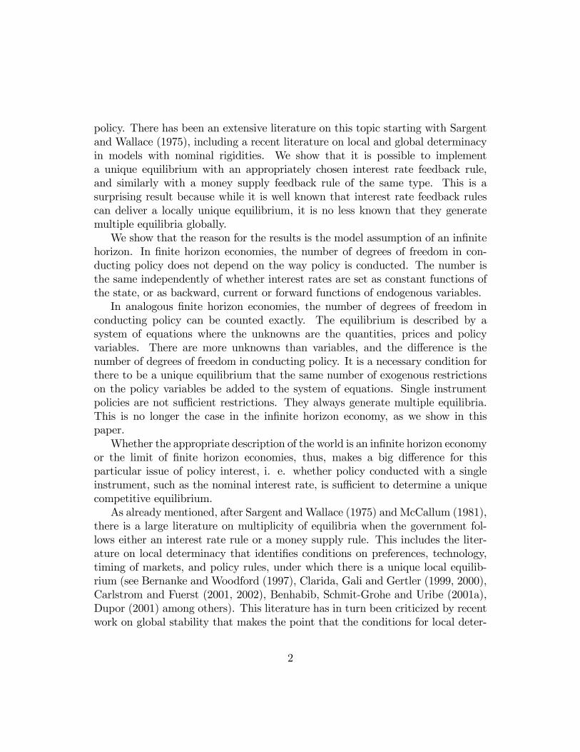
policy. There has been an extensive literature on this topic starting with Sargentand Wallace (1975), including a recent literature on local and global determinacyin models with nominal rigidities. We show that it is possible to implementa unique equilibrium with an appropriately chosen interest rate feedback rule,and similarly with a money supply feedback rule of the same type. This is asurprising result because while it is well known that interest rate feedback rulescan deliver a locally unique equilibrium, it is no less known that they generatemultiple equilibria globally.We show that the reason for the results is the model assumption of an in�nite

horizon. In �nite horizon economies, the number of degrees of freedom in con-ducting policy does not depend on the way policy is conducted. The number isthe same independently of whether interest rates are set as constant functions ofthe state, or as backward, current or forward functions of endogenous variables.In analogous �nite horizon economies, the number of degrees of freedom in

conducting policy can be counted exactly. The equilibrium is described by asystem of equations where the unknowns are the quantities, prices and policyvariables. There are more unknowns than variables, and the di¤erence is thenumber of degrees of freedom in conducting policy. It is a necessary condition forthere to be a unique equilibrium that the same number of exogenous restrictionson the policy variables be added to the system of equations. Single instrumentpolicies are not su¢ cient restrictions. They always generate multiple equilibria.This is no longer the case in the in�nite horizon economy, as we show in thispaper.Whether the appropriate description of the world is an in�nite horizon economy

or the limit of �nite horizon economies, thus, makes a big di¤erence for thisparticular issue of policy interest, i. e. whether policy conducted with a singleinstrument, such as the nominal interest rate, is su¢ cient to determine a uniquecompetitive equilibrium.As already mentioned, after Sargent andWallace (1975) and McCallum (1981),

there is a large literature on multiplicity of equilibria when the government fol-lows either an interest rate rule or a money supply rule. This includes the liter-ature on local determinacy that identi�es conditions on preferences, technology,timing of markets, and policy rules, under which there is a unique local equilib-rium (see Bernanke and Woodford (1997), Clarida, Gali and Gertler (1999, 2000),Carlstrom and Fuerst (2001, 2002), Benhabib, Schmit-Grohe and Uribe (2001a),Dupor (2001) among others). This literature has in turn been criticized by recentwork on global stability that makes the point that the conditions for local deter-

2

minacy are also conditions for global indeterminacy (see Benhabib, Schmit-Groheand Uribe (2001b) and Christiano and Rostagno, 2002).Our modelling approach is close to Adao, Correia and Teles (2003) for the case

with sticky prices. In this paper we show that even at the optimal zero interestrate rule there is still room for policy to improve welfare since it is possible to usemoney supply to implement the optimal allocation in a large set of implementableallocations. This paper is also close to Adao, Correia and Teles (2004) wherewe show that it is possible to implement unique equilibria in environments with�exible prices and prices set in advance by pegging state contingent interest ratesas well as the initial money supply. Bloise, Dreze and Polemarchakis (2004) andNakajima and Polemarchakis (2005) are also related research.We assume that �scal policy is endogenous. Exogeneity of �scal policy could

be used, as in the �scal theory of the price level to determine unique equilibria.The paper proceeds as follows: In Section 2, we consider a simple cash in

advance economy with �exible prices. In Section 3 we analyze a simple exampleto discuss the properties of the equilibria obtained when a single monetary policyinstrument is used. In Section 4, we show that there are single instrument feedbackrules that implement a unique equilibrium. In Section 5 we show that in analogous�nite horizon environments the single instrument rules would generate multipleequilibria. In Section 6, we show that the results generalize to the case whereprices are set in advance. Section 7 contains concluding remarks.

2. A model with �exible prices

We �rst consider a simple cash in advance economy with �exible prices. Theeconomy consists of a representative household, a representative �rm behavingcompetitively, and a government. The uncertainty in period t � 0 is describedby the random variable st 2 St and the history of its realizations up to period t(state or node at t), (s0; s1; :::; st), is denoted by st 2 St. The initial realization s0is given. We assume that the history of shocks has a discrete distribution. Thenumber of states in period t is �t.Production uses labor according to a linear technology. We impose a cash-

in-advance constraint on the households�transactions with the timing structuredescribed in Lucas and Stokey (1983). That is, each period is divided into twosubperiods, with the assets market operational in the �rst subperiod and the goodsmarket in the second.

3

2.1. Competitive equilibria

Households The households have preferences over consumption Ct, and leisureLt, described by the expected utility function:

U = E0

( 1Xt=0

�tu (Ct; Lt)

)(2.1)

where � is a discount factor. The households start period t with nominal wealthWt: They decide to hold money, Mt, and to buy Bt nominal bonds that pay RtBtone period later. Rt is the gross nominal interest rate at date t. They also buyBt;t+1 units of state contingent nominal securities. Each security pays one unit ofmoney at the beginning of period t + 1 in a particular state. Let Qt;t+1 be thebeginning of period t price of these securities normalized by the probability ofthe occurrence of the state. Therefore, households spend EtQt;t+1Bt;t+1 in statecontingent nominal securities. Thus, in the assets market at the beginning ofperiod t they face the constraint

Mt +Bt + EtQt;t+1Bt;t+1 �Wt (2.2)

Consumption must be purchased with money according to the cash in advanceconstraint

PtCt �Mt: (2.3)

At the end of the period, the households receive the labor incomeWtNt; whereNt = 1 � Lt is labor and Wt is the nominal wage rate and pay lump sum taxes,Tt. Thus, the nominal wealth households bring to period t+ 1 is

Wt+1 =Mt +RtBt +Bt;t+1 � PtCt +WtNt � Tt (2.4)

The households�problem is to maximize expected utility (2.1) subject to therestrictions (2.2), (2.4), (3.4), together with a no-Ponzi games condition on theholdings of assets.The following are �rst order conditions of the households problem:

uL(t)

uC (t)=Wt

Pt

1

Rt(2.5)

uC (t)

Pt= RtEt

��uC(t+ 1)

Pt+1

�(2.6)

4

Qt;t+1 = �uC(t+ 1)

uC(t)

PtPt+1

, t � 0 (2.7)

From these conditions we get EtQt;t+1 = 1Rt.Condition (2.5) sets the intratem-

poral marginal rate of substitution between leisure and consumption equal to thereal wage adjusted for the cost of using money, Rt. Condition (2.6) is an in-tertemporal marginal condition necessary for the optimal choice of risk-free nom-inal bonds. Condition (2.7) determines the price of one unit of money at timet + 1, for each state of nature st+1, normalized by the conditional probability ofoccurrence of state st+1, in units of money at time t.

Firms The �rms are competitive and prices are �exible. The production func-tion of the representative �rm is linear

Yt � AtNtThe equilibrium real wage is

Wt

Pt= At: (2.8)

Government The policy variables are taxes, Tt, interest rates, Rt, money sup-plies, Mt, state noncontingent public debt, Bt. We can de�ne a policy as a map-ping for the policy variables fTt; Rt;Mt; Bt, t � 0, all stg, that maps sequences ofquantities, prices and policy variables into sets of sequences of the policy variables.De�ning a policy as a correspondence allows for the case where the governmentis not explicit about some of the policy variables. Lucas and Stokey (1983) de�nepolicy as sequences of numbers for some of the variables. Adao, Correia and Teles(2003) de�ne policy as sequences of numbers for all the policy variables. Herewe allow for more generic functions (correspondences) for all the policy variables.We do not allow for targeting rules that can be de�ned as mappings from prices,quantities and policy variables to prices and quantities.The period by period government budget constraints are

Mt +Bt =Mt�1 +Rt�1Bt�1 + Pt�1Gt�1 � Pt�1Tt�1, t � 0Let Qt+1 � Q0;t+1, with Q0 = 1. If limT!1EtQT+1WT+1 = 0

1Xs=0

EtQt;t+s+1Mt+s (Rt+s � 1) =Wt +1Xs=0

EtQt;t+s+1Pt+s [Gt+s � Tt+s] (2.9)

5

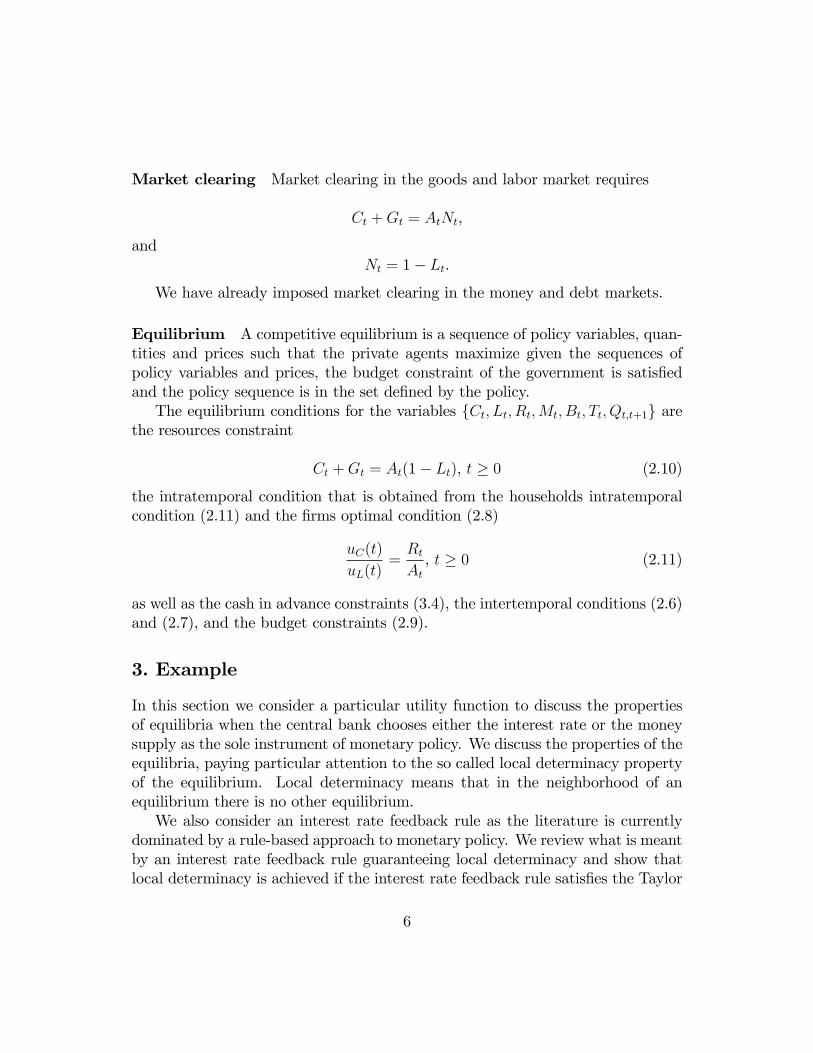
Market clearing Market clearing in the goods and labor market requires

Ct +Gt = AtNt,

andNt = 1� Lt.

We have already imposed market clearing in the money and debt markets.

Equilibrium A competitive equilibrium is a sequence of policy variables, quan-tities and prices such that the private agents maximize given the sequences ofpolicy variables and prices, the budget constraint of the government is satis�edand the policy sequence is in the set de�ned by the policy.The equilibrium conditions for the variables fCt; Lt; Rt;Mt; Bt; Tt; Qt;t+1g are

the resources constraint

Ct +Gt = At(1� Lt), t � 0 (2.10)

the intratemporal condition that is obtained from the households intratemporalcondition (2.11) and the �rms optimal condition (2.8)

uC(t)

uL(t)=RtAt, t � 0 (2.11)

as well as the cash in advance constraints (3.4), the intertemporal conditions (2.6)and (2.7), and the budget constraints (2.9).

3. Example

In this section we consider a particular utility function to discuss the propertiesof equilibria when the central bank chooses either the interest rate or the moneysupply as the sole instrument of monetary policy. We discuss the properties of theequilibria, paying particular attention to the so called local determinacy propertyof the equilibrium. Local determinacy means that in the neighborhood of anequilibrium there is no other equilibrium.We also consider an interest rate feedback rule as the literature is currently

dominated by a rule-based approach to monetary policy. We review what is meantby an interest rate feedback rule guaranteeing local determinacy and show thatlocal determinacy is achieved if the interest rate feedback rule satis�es the Taylor

6

principle. The Taylor principle is veri�ed if in response to an increase in in�ationthe increase in the nominal interest rate is higher.

To simplify the presentation we takeGt = 0 and the utility function u (Ct; Lt) =Ct+v (Lt) ; with v (Lt) increasing in Lt, limLt!0 v

0 (Lt) =1 and limLt!1 v0 (Lt) =

0. We consider 3 monetary policies: a constant interest rate, a constant growthrate for the money supply and an interest rate feedback rule. For the sake of sim-plicity we consider the deterministic environment, i.e. st = st+1 for all t. Thestochastic environment is considered in the appendix.The equilibrium conditions for the variables fCt; Lt; Pt;Mt; Rtg are: the house-

hold�s intratemporal and intertemporal conditions

1

v0 (Lt)=RtA

(3.1)

and1

Pt= Rt�

1

Pt+1; (3.2)

the feasibility conditionCt = A(1� Lt); (3.3)

and the cash in advance condition

Mt � PtCt; with equality if Rt > 1: (3.4)

It will be useful for the discussion below to remember that from (3.1) and (3.3)there is a positive relation between Lt and Rt and a negative relation between Ctand Lt:

3.1. Constant interest rate

Here we assume that the central bank chooses to maintain a constant interestrate equal to R � 1: In this case Ct and Lt are pin down by (3.1) and (3.3).The in�ation, �t, is pin down by (3.2), �t = R�. Any positive real number is anequilibrium P0. Thus, there is a multiplicity of equilibrium price sequences andas a consequence from (3.4) a multiplicity of equilibrium money sequences. Theliterature has a jargon for this result, it is said that the outcome of setting theinterest rate is real determinacy and nominal indeterminacy. All the equilibria arelocally undetermined as for any equilibrium price level there is another equilibriumprice level in its neighborhood. In a stochastic environment with nominal frictions,

7

like sticky prices or sticky wages, the monetary policy of setting the interest rateis less interesting since it leads to multiplicity of the real allocations. We clarifythis issue in the appendix.

3.2. Constant money growth

Here we study the equilibria when the central bank chooses M0 and a constantrate of money growth of the form Mt = �tM0, where � > 1

�: There are many

equilibria. In order to show that, we �nd it useful to de�ne real money asmt � Mt

Pt;

and replace (3.1) in (3.2)

mt+1 = �(Lt)mt, where �(Lt) =�v0 (Lt)

A�: (3.5)

There are two steady states: one with mt+1

mt= 1; Rt =

��> 1; Ct and Lt (= L)

that solve (3.1) and (3.3) for Rt = ��, and Pt satisfying (3.4) with equality. There

is another steady state with Rt = 1; Ct and Lt (= eL) that solve (3.1) and (3.3)for Rt = 1;

mt+1

mt= �

�eL� > 1 and Pt+1Pt

= �

�(eL) . In this steady state in�ation isdetermined but the initial price level is not since (3.4) may not be binding whenRt = 1.The remaining equilibria can be divided according to the value of leisure in

period zero, L0: There are many equilibria with L0 > L. From (3.5) we getm1

m0= �(L0) < 1. Thus, from (3.3) and the fact that (3.4) holds with equality

in period 1 we obtain L1 < L0 which implies �(L1) < �(L0) : Proceeding inthis way we obtain mt and Ct approaching zero and Lt approaching 1: From (3.1)and the fact that mt approaches zero we obtain Rt and Pt approaching in�nity.In�ation Pt+1

Pt= �

�(Lt)approaches in�nity as the denominator approaches zero.

There are also equilibria with eL < L0 < L: By (3.1), R0 > 1, which meansthat (3.4) holds with equality. From (3.5), (3.3) and the assumption that mt = ctwe get sequences fLt; Ct;mtg. Let t� be the �rst period such that Lt� obtainedfrom the process just described satis�es (3.1) with Rt � 1: The elements of thesequence up to t� are part of the equilibrium, but the ones after are not. In periodt� (3.4) does not hold with equality which implies that Rt� = 1: This means thatin periods t�; t� + 1; t� + 2; ::: the equilibrium Lt must satisfy (3.1) for Rt = 1;

which we denoted by eL and the equilibrium Ct solves (3.3) for Lt = eL: Alsomt+1

mt= �

�eL� > 1 for t � t�; and in�ation is constant, Pt+1Pt= �

�(eL) for t � t�, mt

approaches in�nity and Pt approaches zero.

8

The steady state associated with Rt = ��, for all t; is locally determined and

the steady state associated with Rt = 1, for all t; is locally undetermined.

3.3. Interest rate feedback rule

Now we study the equilibria when the central bank follows an interest rate feed-back rule. Let R be a steady state equilibrium interest rate and let � be thecorresponding steady state equilibrium in�ation rate. Then, R = �

�, where 1

�

is the real interest rate. Assume that the central bank conducts a pure currentnonlinear Taylor rule:1

Rt = R��t�

���;

where �� � 1 (the Taylor principle), and �t � PtPt�1

. After substituting the Taylorrule in the intertemporal condition of the household, (3.2), we get

zt+1 = (zt)��;

where zt = �t�: By recursive substitution we get

zt+k = (zt)k��; for all k and t: (3.6)

There is no condition to pin down the initial value for in�ation. Since the initialin�ation level can be any value there is an in�nity of equilibrium trajectories forthe in�ation rate. Nevertheless, they can be typi�ed in 3 classes. Either in�ationis constant, �t = �, or there is an hyperin�ation, �t �! 1, or in�ation isapproaching zero, �t �! 0. This is easy to verify. If �0 = �; then (3.6) impliesthat �t = � for all t: If �0 > �; then (3.6) implies that �t+1 > �t and �t �! 1;since �� > 1: If �0 < �; then (3.6) implies that �t+1 < �t and �t �! 0; since�� > 1:Thus, when the central bank follows a Taylor rule that obeys the Taylor prin-

ciple it is able to get local determinacy. In a neighborhood of the steady statein�ation � there is no other equilibrium in�ation trajectory. But we have justseen that there is an in�nity of other equilibria for in�ation which converge to zero

1Usually the Taylor rule is presented in its linearized form. As can be veri�ed the linearizedversion is,

Rt � R = � (�t ��) :

9

or to in�nity. These results beg two interrelated questions: Why is local deter-minacy such an interesting property? Or why has most of the literature assumedthat undesirable equilibria do not happen? We do not know the answer to thesequestions.It is easy to verify, using an argument similar to the one above, that if the

Taylor rule did not obey the Taylor principle, i.e. �� < 1, there would be just twotypes of equilibrium. The steady state and an in�nity of equilibria converging tothe steady state. At �rst sight it would seem that it would be preferable that acentral bank would follow a Taylor rule that did not satisfy the Taylor principle, as"undesirable" equilibria, hyperin�ations or hyperde�ations would not be possible.This conclusion is not correct because whenever there is multiplicity of equilibriait may be possible that sunspots can cause large �uctuations in in�ation. In�ationcan �uctuate randomly just because agents come to believe this will happen.Why do we get so many equilibria? Is it possible that we are forgeting equilib-

rium conditions? There are no more equilibrium conditions over these variables.The so called transversality conditions are satis�ed since in our economy there aregovernment bonds. Moreover, since our �scal authority has a Ricardian policythe government�s in�nite-horizon budget constraint does not provide additionalinformation. In particular it cannot be used to obtain the initial price level as itis done in the �scal theory of price level literature.There may be institutions that we have ignored in the model, which can be used

to eliminate some of these "undesirable" equilibria. For instance, in some modelsan hyperin�ation can be eliminated if the central bank has su¢ cient real resourcesand can commit to buy back its currency if the price level exceeds a certain level.This is known as fractional real backing of the currency (seeObstfeld and Rogo¤(1983)). We are not going to pursue this issue here.

4. Single instrument feedback rules.

In this section we assume that policy is conducted with either interest rate ormoney supply feedback rules. We show that there are single instrument feedbackrules that implement a unique equilibrium for the allocation and prices. Theproposition for an interest rate feedback rule follows:

Proposition 4.1. When the �scal policy is endogenous and monetary policy is

10

conducted with the interest rate feedback rule

Rt =�t

Et�uC(t+1)Pt+1

;

�t is an exogenous variable, there is a unique equilibrium.

Proof: Suppose policy is conducted with the interest rate feedback rule Rt =�t

Et�uC (t+1)

Pt+1

. Then the intertemporal and intratemporal conditions, (2.6) and (2.11)

can be written asuC(t)

Pt= �t, t � 0 (4.1)

uC(t)

uL(t)=

�t�Et�t+1

At, t � 0 (4.2)

These conditions together with the cash in advance conditions, (3.4), and theresource constraints, (2.10), determine uniquely the variables Ct, Lt, Pt and Mt.The budget constraints (4.4) are satis�ed for multiple paths of the taxes and

state noncontingent debt levels�The forward looking interest rate feedback rules that guarantee uniqueness of

the equilibrium resemble the rules that appear to be followed by central banks.The nominal interest rate reacts positively both to the forecast of future consump-tion and to the forecast of the future price level. In this there is a di¤erence to thefeedback rules that are usually considered in that it depends on the future pricelevel rather than in�ation.Depending on the exogenous process for �t, with this feedback rule it is possible

to decentralize any feasible allocation distorted by the nominal interest rate. The�rst best allocation, at the Friedman rule of a zero nominal interest rate, can alsobe implemented. With �t =

1�t, t � 0, condition (4.2) becomes

uC(t)

uL(t)=1

At, t � 0

which, together with the resource constraint (2.10) gives the �rst best allocationCt = C(At; Gt), Lt = L(At; Gt). The price level Pt = P (At; Gt) can be obtainedusing (4.1), i.e.

uC(C(:); L(:))

Pt=1

�t, t � 0;

11

and the money supply is obtained using the cash-in-advance constraint, Mt =P (At; Gt)C(At; Gt).Allocations where in�ation is zero can also be implemented even if in this �ex-

ible price environment they are not desirable. There are multiple such allocationswith nominal interest rates satisfying

Rt =uC(C(At; Gt; Rt); L(At; Gt; Rt))

�EtuC(C(At+1; Gt+1; Rt+1); L(At+1; Gt+1; Rt+1)), t � 0

where the functions C and L are the solution for Ct and Lt of the system ofequations given by (2.11) and (2.10).For each path of the nominal interest rate, fRtg, associated with zero in�ation,

there is a unique path for f�tg up to a constant term,

uC(C(At; Gt; Rt); L(At; Gt; Rt))

P= �t, t � 0.

In an economy where the use of money is becomes negligible which correspondsto a cash-in-advance condition

vtPtCt �Mt: (4.3)

where vt ! 0, there is a single path for the nominal interest rate consistent withzero in�ation,

Rt =uC(C(At; Gt); L(At; Gt))

�EtuC(C(At+1; Gt+1); L(At+1; Gt+1)), t � 0

An analogous proposition to Proposition 3.1 is obtained when policy is con-ducted with a particular money supply feedback rule.

Proposition 4.2. When the �scal policy is endogenous and the policy is con-ducted with the money supply feedback rule,

Mt =�Rt�1CtuC(t)

�t�1

there is a unique equilibrium.

12

Proof: Suppose policy is conducted according to the money supply ruleMt =�Rt�1CtuC(t)

�t�1. Then, the equilibrium conditions

PtCt =�Rt�1CtuC(t)

�t�1

obtained using the cash in advance conditions (3.4),

uC(t)

Pt= �t

obtained from the intertemporal conditions (2.6), in addition to the resource con-straints, (2.10) and the intratemporal conditions (2.11) determine uniquely thefour variables, Ct, ht, Pt, Rt in each period t � 0 and state st.The taxes and debt levels satisfy the budget constraint (4.4)�The result that there are single instrument feedback rules that implement a

unique equilibrium is a surprising one. In fact it is well known that interest raterules may implement a determinate equilibrium, but not a unique global equilib-rium. To illustrate this, consider the case where monetary policy is conductedwith constant functions for the policy variables. We will show that in that casean interest rate policy generates multiple equilibria. That result is directly ex-tended to the case where the interest rate is a function of contemporaneous orpast variables.

4.1. Conducting policy with constant functions.

In this section, we show that in general when policy is conducted with constantfunctions for the policy instruments, it is necessary to determine exogenously bothinterest rates and money supplies.The equilibrium conditions are the resources constraints, (2.10), the intratem-

poral conditions (2.11), the cash in advance constraints (3.4), the intertemporalconditions (2.6) and the budget constraints (2.9) that can be written as

Et

1Xs=0

�suC(t+ s)Ct+s

�Rt+s � 1Rt+s

�= uC(t)

Wt

Pt+Et

1Xs=0

�suC(t+ s)[Gt+s � Tt+s]

Rt+s(4.4)

using (2.7).These conditions de�ne a set of equilibrium allocations, prices and policy vari-

ables. There are many equilibria. We want to determine conditions on the ex-ogeneity of the policy variables such that there is a unique equilibrium in the

13

allocation and prices. We �rst consider the case in which a policy are sequencesof numbers for money supplies and interest rates.From the resources constraints,(2.10), the intratemporal conditions (2.11), and

the cash in advance constraints, (3.4), we obtain the functions Ct = C(Rt) andLt = L(Rt) and Pt = Mt

C(Rt), t � 0. As long as uC(Ct; Lt)Ct depends on Ct or

Lt, excluding therefore preferences that are additively separable and logarithmicin consumption, the system of equations can be summarized by the followingdynamic equations:

uC(C(Rt); L(Rt))Mt

C(Rt)

= �RtEt

"uC(C(Rt+1); L(Rt+1))

Mt+1

C(Rt+1)

#, t � 0 (4.5)

together with the budget constraints, (4.4).Suppose the path of money supply is set exogenously in every date and state.

In addition, in period zero the interest rate, R0, is set exogenously and, for eacht � 1, for each state st�1, the interest rates are set exogenously in #St� 1 states.In this case there is a single solution for the allocations and prices. Similarly,there is also a unique equilibrium if the nominal interest rate is set exogenously inevery date and state, and so is the money supply in period 0, M0, as well as, foreach t � 1, and for state st�1, the money supply in #St � 1 states. The budgetconstraints restrict, not uniquely, the taxes and debt levels.The proposition follows

Proposition 4.3. Suppose policy are constant functions. In general, if moneysupply is determined exogenously in every date and state, and if interest rates arealso determined exogenously in the initial period, as well as in �t��t�1 states foreach t � 1, then the allocations and prices can be determined uniquely. Similarly,if the exogenous policy instruments are the interest rates in every state, the initialmoney supply and the money supply, in �t � �t�1 states, for t � 1, then there isin general a unique equilibrium.

The proposition states a general result. In the particular case where the prefer-ences are additively separable and logarithmic in consumption, and money supplyis set exogenously in every state, there is a unique equilibrium in the allocationsand prices. There is no need to set exogenously the interest rates as well. Thisexample is helpful in understanding the main point of the paper, that the degreesof freedom in conducting policy depend on how policy is conducted and on othercharacteristics of the environment.

14

4.2. Current or backward interest rate feedback rules .

We have shown Proposition 3.3. assuming that policy was conducted with con-stant functions for the policy variables. However, the use of interest rate rulesthat depend on current or past variables clearly preserves the same degrees offreedom in the determination of policy, as identi�ed in that proposition. When�scal policy is endogenous, it is still necessary to determine exogenously the levelsof money supply in some but not all states. The corollary follows

Corollary 4.4. When policy is conducted with current or backward interest ratefeedback rules and �scal policy is endogenous, there is a unique equilibrium if themoney supply is set exogenously in #St � 1 states, for each state st�1, t � 1, aswell M0.

5. Robustness: Finite horizon.

We have shown in the previous section that there are interest rate rules thatimplement a unique equilibrium but that current or backward feedback rules donot. This means that even if the same number of instruments is set exogenously,the remaining degrees of freedom in determining policy depend on how thosedegrees of freedom are �lled. This happens because the model economy has anin�nite horizon.If the economy had a �nite horizon it would be characterized by a �nite number

of equations and unknowns. In that case the number of degrees of freedom inconducting policy is a �nite number that does not depend on whether policy isconducted with constant functions, functions of future, current or past variables,as long as these functions are truly exogenous, i.e. independent from the remainingequilibrium conditions.To determine the degrees of freedom in the case of a �nite horizon economy

amounts to simply counting the number of equations and unknowns. We proceedto considering the case where the economy lasts for a �nite number of periodsT +1, from period 0 to period T . After T , there is a subperiod for the clearing ofdebts, where money can be used to pay debts, so that

WT+1 =MT +RTBT + PTGT � PTTT = 0

The �rst order conditions in the �nite horizon economy are the intratemporalconditions, (2.11) for t = 0; :::; T , the cash in advance constraints, (3.4) also for

15

t = 0; :::; T , the intertemporal conditions

uC (t)

Pt= RtEt

��uC(t+ 1)

Pt+1

�, t = 0; :::; T � 1

Qt;t+1 = �uC(t+ 1)

uC(t)

PtPt+1

, t = 0; :::; T � 1 (5.1)

and, for any 0 � t � T , and state st, the budget constraints

T�tXs=0

EtQt;t+s+1Mt+s (Rt+s � 1) =Wt +

T�tXs=0

EtQt;t+s+1Pt+s [Gt+s � Tt+s]

where E0QT+1 � E0QTRT

.The budget constraints restrict, not uniquely, the levels of state noncontingent

debts and taxes. Assuming these policy variables are not set exogenously we canignore this restriction. The equilibrium can then be summarized by

uC(C(Rt); L(Rt))Mt

C(Rt)

= �RtEt

"uC(C(Rt+1); L(Rt+1))

Mt+1

C(Rt+1)

#, t = 0; :::; T � 1 (5.2)

Note that the total number of money supplies and interest rates is the same.There are �0 + �1 + ::: + �T of each monetary policy variable. The number ofequations is �0 + �1 + ::: + �T�1. In order for there to be a unique equilibriumneed to add to the system �0 + �1 + ::: + 2�T independent restrictions. Onepossibility is to set exogenously the interest rates in every state and in additionthe money supply in every terminal node. Similarly there is a unique equilibriumif the money supply is set exogenously in every state and the interest rates are setin every terminal node. In this sense, the two monetary instruments are equivalentin this economy.When policy is conducted with the forward looking feedback rule in Section 2,

the policy for the interest rate in the terminal period RT , cannot be a function ofvariables in period T + 1. If these rates are exogenous constants, it still remainsto determine the money supply in every state at T .In this �nite horizon economy there is an exact measure for the degrees of

freedom in conducting policy. In an economy that lasts from t = 0 to t = T ,

16

these are �0+�1+ :::+2�T . This measure does not depend on how policy is con-ducted, whether with constant functions or functions of endogenous variables, andit also does not depend on price setting restrictions. The price setting restrictionsintroduce as many variables as number of restrictions.

6. Robustness: Price setting restrictions

In this section we show that the results derived above extend to an environmentwith prices set in advance. We modify the environment to consider price settingrestrictions. There is a continuum of goods, indexed by i 2 [0; 1] : Each good iis produced by a di¤erent �rm. The �rms are monopolistic competitive and setprices in advance with di¤erent lags.The households have preferences described by (2.5) where Ct is now the com-

posite consumption

Ct =

�Z 1

0

ct(i)��1� di

� ���1

; � > 1:

Households have a demand function for each good given by

ct (i) =

�pt (i)

Pt

���Ct:

where Pt is the price level,

Pt =

�Zpt(i)

1��di

� 11��

. (6.1)

The households�intertemporal and intratemporal conditions are as before, (2.5),(2.6) and (2.7).The government must �nance an exogenous path of government purchases

fGtg1t=0, such that

Gt =

�Z 1

0

gt(i)��1� di

� ���1

; � > 0 (6.2)

Given the prices on each good i in units of money, Pt(i), the government minimizesexpenditure on government purchases by deciding according to

gt(i)

Gt=

�pt(i)

Pt

���(6.3)

17

The resource constraints can be written as

(Ct +Gt)

Z 1

0

�pt (i)

Pt

���di = AtNt: (6.4)

We consider now that �rms set prices in advance. A fraction �j �rms set pricesj periods in advance with j = 0; :::J � 1: Firms decide the price for period t withthe information up to period t� j to maximize:

Et�j [Qt�j;t+1 (pt(i)yt(i)�Wtnt(i))]

subject to the production function

yt(i) � Atnt(i)

and the demand function

yt(i) =

�pt(i)

Pt

���Yt (6.5)

where yt(i) = ct(i) + gt(i)The optimal price is

pt(i) = pt;j =�

(� � 1)Et�j��t;jWt

At

�where

�t;j =Qt�j;t+1P

�t Yt

Et�j�Qt�j;t+1P �t Yt

� :The price level at date t can be written as

Pt =

"J�1Pj=0

�j (pt;j)1��

# 11��

(6.6)

When we compare the two sets of equilibrium conditions, under �exible andprices set in advance, here we are adding more variables, the prices of the dif-ferently restricted �rms, but we also add the same number of equations. Thisargument works in this case, because we can write the new equations as functionsof current and past variables.

18

7. Concluding Remarks

The problem of multiplicity of equilibria under an interest rate policy has been ad-dressed, after Sargent and Wallace (1975) and McCallum (1981), by an extensiveliterature on determinacy under interest rate rules. Interest rate feedback ruleson endogenous variables such as the in�ation rate can, with appropriately chosencoe¢ cients, deliver determinate equilibria. There are still multiple equilibria butonly one of those equilibria stays in the proximity of a steady state.In this paper we show that in a simple monetary model with �exible prices or

prices set in advance there are interest rate feedback rules, and also money supplyfeedback rules, that implement unique equilibria. The interest rate feedback rulesare forward rules that resemble the policy rules that central banks follow.The results are not robust to the following change in the theoretical environ-

ment. The model economy has an in�nite horizon. Suppose that we consideredinstead the analogous �nite horizon economy. In that economy, for an arbitrar-ily large horizon, single instrument feedback rules would not implement uniqueequilibria.

8. Appendix

Here we consider the example of section 3 in a stochastic environment and an-alyze the constant interest rate policy and the interest rate feedback rule. Theequilibrium conditions for the stochastic case are (3.1), (3.3), (3.4) and

1

Pt= Rt�Et

1

Pt+1: (8.1)

From the deterministic to the stocastic framework only the intertemporal condi-tion changes, all the remaining conditions remain the same.

8.1. Constant interest rate

Here we assume that the central bank chooses to mantain a constant interest rateequal to R � 1: As in the deterministic case Ct and Lt are pin down by (3.1) and(3.3). Now it is the expected in�ation, �t, that is pin down by (3.2), Et�t+1 =R�. There are many distributions of realized in�ation that are compatible withthat expected in�ation and all can be part of an equilibrium. There is as wella multiplicity of equilibrium price sequences and as a consequence from (3.4) amultiplicity of equilibrium money sequences.

19

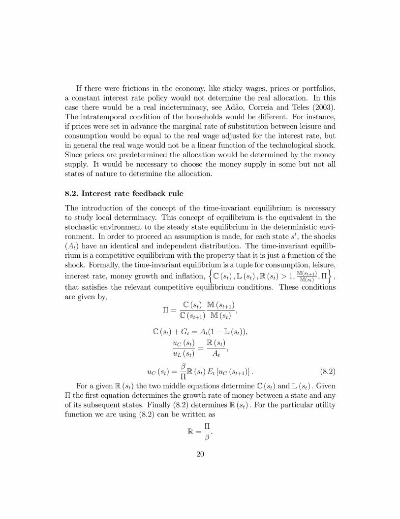
If there were frictions in the economy, like sticky wages, prices or portfolios,a constant interest rate policy would not determine the real allocation. In thiscase there would be a real indeterminacy, see Adão, Correia and Teles (2003).The intratemporal condition of the households would be di¤erent. For instance,if prices were set in advance the marginal rate of substitution between leisure andconsumption would be equal to the real wage adjusted for the interest rate, butin general the real wage would not be a linear function of the technological shock.Since prices are predetermined the allocation would be determined by the moneysupply. It would be necessary to choose the money supply in some but not allstates of nature to determine the allocation.

8.2. Interest rate feedback rule

The introduction of the concept of the time-invariant equilibrium is necessaryto study local determinacy. This concept of equilibrium is the equivalent in thestochastic environment to the steady state equilibrium in the deterministic envi-ronment. In order to proceed an assumption is made, for each state st, the shocks(At) have an identical and independent distribution. The time-invariant equilib-rium is a competitive equilibrium with the property that it is just a function of theshock. Formally, the time-invariant equilibrium is a tuple for consumption, leisure,interest rate, money growth and in�ation,

nC (st) ;L (st) ;R (st) > 1; M(st+1)M(st) ;�

o;

that satis�es the relevant competitive equilibrium conditions. These conditionsare given by,

� =C (st)C (st+1)

M (st+1)M (st)

;

C (st) +Gt = At(1� L (st));uC (st)

uL (st)=R (st)At

;

uC (st) =�

�R (st)Et [uC (st+1)] : (8.2)

For a given R (st) the two middle equations determine C (st) and L (st) : Given� the �rst equation determines the growth rate of money between a state and anyof its subsequent states. Finally (8.2) determines R (st) : For the particular utilityfunction we are using (8.2) can be written as

R =�

�:

20

That is the time-invariant nominal interest rate does not depend on the shocks.Suppose that the central bank conducts a pure current Taylor rule:

Rt = R��t�

���; (8.3)

where �� � 1 (the Taylor principle), and �t = PtPt�1

.After substituting (8.3) in the households�intertemporal condition, we get

Et�z�1t+1

�=�z�1t���; (8.4)

where zt = �t�: By recursive substitution we get�

Et

�nEt+1

h:::�Et+k�1z

�1t+k

� 1�� :::

io 1��

�� 1��

= z�1t ; for all k; t (8.5)

In the following paragraph we supply an heuristic proof that the only equilibriaare the time-invariant equilibrium and an in�nity of other equilibria which havethe characteristic that in some states of nature either in�ation is going to in�nityor is going to zero.Since �� > 1; if z�1t > 1 then z�1t ! 1 with positive probability. The

proof is by contradiction. Assume it was not converging to in�nity with positiveprobability, then it would be bounded with probability one, which means that nomatter how arbitrary in the future you take the z�1t+s its expected value would bebounded with probability one. But since the exponent is a constant smaller thanone by taking s su¢ ciently large will get the left hand side of (8.5) smaller thanthe right hand side. By a similar argument if z�1t < 1; have z�1t ! 0 with positiveprobability.Thus, when the central bank follows a Taylor rule that obeys the Taylor prin-

ciple it is able to get local determinacy. In a neighborhood of the time-invariantequilibrium with in�ation � there is no other equilibrium. We have just seenthat the other equilibria which are in�nite in number are either associated within�ation converging with probability bounded from zero to in�nity or to zero.

References

[1] B. Adão, I. Correia and P. Teles, 2003, �Gaps and Triangles,� Review ofEconomic Studies 70, 4, 699-713.

21

[2] B. Adão, I. Correia and P. Teles, 2004, �Monetary Policy with State-Contingent Interest Rates�, working paper, Federal Reserve Bank ofChicago.

[3] J. Benhabib, S. Schmitt�Grohe and M. Uribe, 2001a, �Monetary Policy andMultiple Equilibria,�American Economy Review 91, 167-185.

[4] J. Benhabib, S. Schmitt�Grohe and M. Uribe, 2001b, �The Perils of TaylorRules,�Journal of Economic Theory 96, 40-69.

[5] B. Bernanke and M. Woodford, 1997, �In�ation Forecasts and MonetaryPolicy�, Journal of Money, Credit and Banking 24, 653-684.

[6] G. Bloise, J. Dreze and H. Polemarchakis, 2004, �Monetary Equilibria overan In�nite Horizon,�Economic Theory 25.

[7] C. T. Carlstrom and T. S. Fuerst, 2002, �Taylor Rules in a Model thatSatis�es the Natural Rate Hypothesis�, American Economic Review 92,79-84.

[8] C. T. Carlstrom C. T. and T. S. Fuerst, 2001, �Timing and Real Indetermi-nacy in Monetary Models,�Journal of Monetary Economics 47, 285-298.

[9] L. Christiano and M. Rostagno (2002),.�Money Growth, Monitoring and theTaylor Rule,�mimeo, Northwestern University.

[10] R. Clarida, J. Gali and M. Gertler, 1999, �The Science of Monetary Policy:A New Keynesian Perspective�, Journal of Economic Literature 37, 1661-1707.

[11] R. Clarida, J. Gali and M. Gertler, 2000, �Monetary Policy Rules and Macro-economic Stability: Evidence and Some Theory�, Quarterly Journal ofEconomics 115, 147-180.

[12] W. Dupor, 2001, �Investment and Interest Rate Policy,�Journal of EconomicTheory 98, 85-113.

[13] R. E. Lucas, Jr., and N. L. Stokey, 1983, "Optimal Fiscal and MonetaryPolicy in an Economy without Capital," Journal of Monetary Economics12, 55-93.

[14] B. McCallum, 1981, �Price Level Determinacy with an Interest Rate PolicyRule and rational Expectations,�Journal of Monetary Economics 8, 319-329.

22

[15] T. Nakajima and H. Polemarchakis, 2005, �Money and Prices under Uncer-tainty,�Review of Economic Studies 72.

[16] Obstfeld and Rogo¤, (1983), �Speculative Hyperin�ations in MaximizingModels: Can We Rule Them Out�, Journal of Political Economy, 91,675-687.

[17] T. J. Sargent and N. Wallace, 1975, �Rational Expectations, the OptimalMonetary Instrument, and the Optimal Money Supply Rule,�Journal ofPolitical Economy 83, 241-254.

23