Embed Size (px)
Citation preview
APPLICATION NOTE
www.aesa-cortaillod.com
Balunless : single ended S-parameters Cable manufacturers detect weak points in their production
The technology of symmetric copper pairs
continues to evolve and ensures transmissions
at ever higher frequencies (e.g. cat 8 or the
upcoming 40GBASE-T). To secure their
specifications, manufacturers shall have suitable
test equipment. AESA has introduced the first
automatic testing equipment with the
"balunless" technology. It opens the door to the
measurement of multiple new parameters.
It is essential to understand and control them
since they offer new opportunities in
measurement technology to help finding the
cause of marginal or failing lots in production by
analysing single-ended S-parameters. This
method allows by mathematical superposition
of single-ended measurements to get the well-
known mixed-mode S-parameters. The purpose
of this application note is to share knowledge
about this method and related parameters.
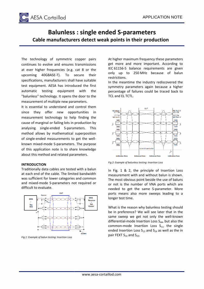
INTRODUCTION Traditionally data cables are tested with a balun at each end of the cable. The limited bandwidth was sufficient for lower categories and common and mixed-mode S-parameters not required or difficult to evaluate.
Fig.1: Example of balun testing: Insertion Loss
At higher maximum frequency these parameters get more and more important. According to IEC 61156-5 balance requirements are given only up to 250 MHz because of balun restrictions. In the meantime the industry rediscovered the symmetry parameters again because a higher percentage of failures could be traced back to TCL and EL TCTL.
Fig.2: Example of balunless testing: Insertion Loss
In Fig. 1 & 2, the principle of Insertion Loss measurement with and without balun is shown. The most obvious point beside the use of baluns or not is the number of VNA ports which are needed to get the same S-parameter. More ports means also more sweeps leading to a longer test time. What is the reason why balunless testing should be in preference? We will see later that in the same sweep we get not only the well-known differential-mode Insertion Loss Sdd, but also the common-mode Insertion Loss Scc, the single ended Insertion Loss S13 and S24 as well as the in pair FEXT S14 and S23.

APPLICATION NOTE
© 2015 AESA Cortaillod. All rights reserved www.aesa-cortaillod.com Page 2 of 7
THEORETICAL BACKGROUND
As described by Fan et al (2003), the key is a conversion of single-ended S-parameters into mixed-mode S-parameters.
Fig.3: 4-Port device (single-ended) Therefore the 4-Port device can be mathematically represented by single-ended S-parameters and the waves going into the DUT (a) and the waves which come out of the DUT (b).
[
𝑏1
𝑏2
𝑏3
𝑏4
] = [
𝑆11 𝑆12 𝑆13 𝑆14
𝑆21 𝑆22 𝑆23 𝑆24
𝑆31 𝑆32 𝑆33 𝑆34
𝑆41 𝑆42 𝑆43 𝑆44
] [
𝑎1
𝑎2
𝑎3
𝑎4
]
Fig.4: single-ended matrix representation In a similar way the same DUT can be represented as a 2-Port differential device:
Fig.5: 2-Port differential device (mixed-mode)
A mixed-mode S-matrix can be organised similarly to the single-ended S-matrix:
[
𝑏𝑑1
𝑏𝑑2
𝑏𝑐1
𝑏𝑐2
] = [
𝑆𝑑𝑑11 𝑆𝑑𝑑12 𝑆𝑑𝑐11 𝑆𝑑𝑐12
𝑆𝑑𝑑21 𝑆𝑑𝑑22 𝑆𝑑𝑐21 𝑆𝑑𝑐22
𝑆𝑐𝑑11 𝑆𝑐𝑑12 𝑆𝑐𝑐11 𝑆𝑐𝑐12
𝑆𝑐𝑑21 𝑆𝑐𝑑22 𝑆𝑐𝑐21 𝑆𝑐𝑐22
] [
𝑎𝑑1
𝑎𝑑2
𝑎𝑐1
𝑎𝑐2
]
Fig.6: 2-Port differential matrix representation With comparison between both cases, single-ended and mixed-mode, the mathematical correlation for each mixed-mode S-parameter can be found and explained by a combination of 4 single-ended S-parameters. The resulting mixed-mode S-matrix consists of differential-mode to differential-mode (yellow), common-mode to common-mode (green) and mixed-mode (common-mode to differential-mode (blue) and differential-mode to common-mode (pink) S-parameters:
𝑆𝑚𝑚 = [
𝑆𝑑𝑑11 𝑆𝑑𝑑12 𝑆𝑑𝑐11 𝑆𝑑𝑐12
𝑆𝑑𝑑21 𝑆𝑑𝑑22 𝑆𝑑𝑐21 𝑆𝑑𝑐22
𝑆𝑐𝑑11 𝑆𝑐𝑑12 𝑆𝑐𝑐11 𝑆𝑐𝑐12
𝑆𝑐𝑑21 𝑆𝑐𝑑22 𝑆𝑐𝑐21 𝑆𝑐𝑐22
]
Fig.7: mixed-mode matrix
Differential-mode to differential-mode Common-mode to differential-mode Differential-mode to common-mode Common-mode to common-mode
As a reading example the following formula can be taken:
𝑅𝐿𝑑𝑑@ 𝑃𝑜𝑟𝑡 1 ∶ 𝑆𝑑𝑑11 =1
2(𝑆11 − 𝑆13 − 𝑆31 + 𝑆33)
𝑆𝑚𝑚 =1
2[[𝑆11 − 𝑆13 − 𝑆31 + 𝑆33 𝑆12 − 𝑆14 − 𝑆32 + 𝑆34
𝑆21 − 𝑆23 − 𝑆41 + 𝑆43 𝑆22 − 𝑆24 − 𝑆42 + 𝑆44] [
𝑆11 + 𝑆13 − 𝑆31 − 𝑆33 𝑆12 + 𝑆14 − 𝑆32 − 𝑆34
𝑆21 + 𝑆23 − 𝑆41 − 𝑆43 𝑆22 + 𝑆24 − 𝑆42 − 𝑆44]
[𝑆11 − 𝑆13 + 𝑆31 − 𝑆33 𝑆12 − 𝑆14 + 𝑆32 − 𝑆34
𝑆21 − 𝑆23 + 𝑆41 − 𝑆43 𝑆22 − 𝑆24 + 𝑆42 − 𝑆44] [
𝑆11 + 𝑆13 + 𝑆31 + 𝑆33 𝑆12 + 𝑆14 + 𝑆32 + 𝑆34
𝑆21 + 𝑆23 + 𝑆41 + 𝑆43 𝑆22 + 𝑆24 + 𝑆42 + 𝑆44]]
Fig.8: transformation matrix between single-ended S-parameters and mixed-mode S-parameters
The transformation matrix is the base of the following discussion and analyses. Explanation to this formula and some others will be given in the following parts with examples.

APPLICATION NOTE
© 2015 AESA Cortaillod. All rights reserved www.aesa-cortaillod.com Page 3 of 7
CASE 1: LOW RL As shown above the RL @ Port 1 is represented by Sdd11:
𝑆𝑑𝑑11 =1
2(𝑆11 − 𝑆13 − 𝑆31 + 𝑆33)
Here we have an example of RL measurement as it can be taken also with baluns.
Fig.9: return Loss measurement of near end pair 2
The measurement shows a Pass with a marginal margin of 0.2 dB. For a cable manufacturer it can be ok but probably he was just lucky to get a Pass. For balun testing the story ends here. It is not possible to further evaluate the cause of the marginal measurement. With the ability of balunless testing the cable manufacturer has much more opportunities to go deeper into single-ended measurements. From the given formula for Return Loss we can find the 4 single-ended S-parameters. S11 and S33 are the single-ended Return Loss measurements of “a” wire and “b” wire of the pair. S13 and S31 are the crosstalk measurements from “a” wire to “b” wire and from “b” wire to “a” wire.
Fig.10: single-ended NEXT measurements S13 and S31
Fig.11: single-ended RL measurements S11 and S33
The overlay of the single-ended NEXT measurements S13 and S31 shows no noteworthy deviation over the whole frequency range. In contrast the single-ended RL measurements S11 and S33 show diverting values at 100 MHz and above. These differences are causing the poor RL performance of near end. In this specific case wire “b” is worse than wire “a”. As written above there are even more opportunities with single-ended measurements. We can also compare the impedances of each wire.
Fig.12: increasing Impedance wire “b”
The final conclusion with access to single-ended S-parameters is imposing itself now: The increasing impedance of wire “b” causes a bad single-ended RL performance which results in a bad differential-mode RL. The access to single-ended S-parameters
revealed the cause of poor performance which
would stay completely hidden with balun based
measurement technology.
APPLICATION NOTE
© 2015 AESA Cortaillod. All rights reserved www.aesa-cortaillod.com Page 4 of 7
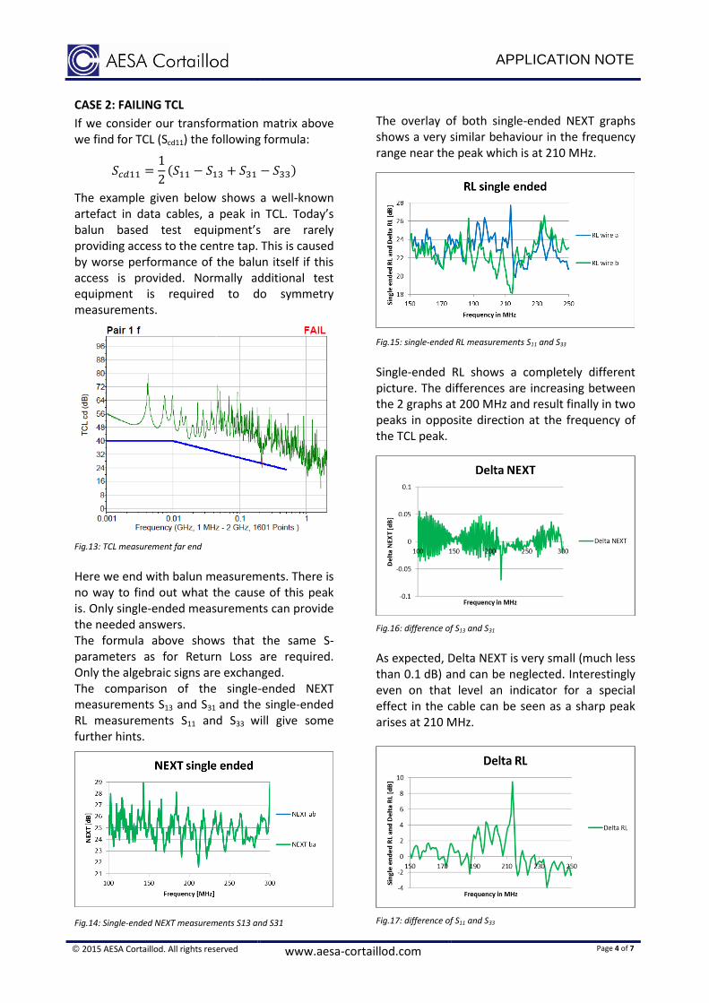
CASE 2: FAILING TCL
If we consider our transformation matrix above we find for TCL (Scd11) the following formula:
𝑆𝑐𝑑11 =1
2(𝑆11 − 𝑆13 + 𝑆31 − 𝑆33)
The example given below shows a well-known artefact in data cables, a peak in TCL. Today’s balun based test equipment’s are rarely providing access to the centre tap. This is caused by worse performance of the balun itself if this access is provided. Normally additional test equipment is required to do symmetry measurements.
Fig.13: TCL measurement far end
Here we end with balun measurements. There is no way to find out what the cause of this peak is. Only single-ended measurements can provide the needed answers. The formula above shows that the same S-parameters as for Return Loss are required. Only the algebraic signs are exchanged. The comparison of the single-ended NEXT measurements S13 and S31 and the single-ended RL measurements S11 and S33 will give some further hints.
Fig.14: Single-ended NEXT measurements S13 and S31
The overlay of both single-ended NEXT graphs shows a very similar behaviour in the frequency range near the peak which is at 210 MHz.
Fig.15: single-ended RL measurements S11 and S33
Single-ended RL shows a completely different picture. The differences are increasing between the 2 graphs at 200 MHz and result finally in two peaks in opposite direction at the frequency of the TCL peak.
Fig.16: difference of S13 and S31
As expected, Delta NEXT is very small (much less than 0.1 dB) and can be neglected. Interestingly even on that level an indicator for a special effect in the cable can be seen as a sharp peak arises at 210 MHz.
Fig.17: difference of S11 and S33
APPLICATION NOTE
© 2015 AESA Cortaillod. All rights reserved www.aesa-cortaillod.com Page 5 of 7
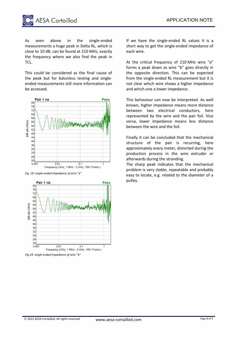
As seen above in the single-ended measurements a huge peak in Delta RL, which is close to 10 dB, can be found at 210 MHz, exactly the frequency where we also find the peak in TCL. This could be considered as the final cause of the peak but for balunless testing and single-ended measurements still more information can be accessed.
Fig. 18: single-ended Impedance of wire “a”
Fig.19: single-ended Impedance of wire “b”
If we have the single-ended RL values it is a short way to get the single-ended impedance of each wire. At the critical frequency of 210 MHz wire “a” forms a peak down as wire “b” goes directly in the opposite direction. This can be expected from the single-ended RL measurement but it is not clear which wire shows a higher impedance and which one a lower impedance. This behaviour can now be interpreted. As well known, higher impedance means more distance between two electrical conductors, here represented by the wire and the pair foil. Vice versa, lower impedance means less distance between the wire and the foil. Finally it can be concluded that the mechanical structure of the pair is recurring, here approximately every meter, distorted during the production process in the wire extruder or afterwards during the stranding. The sharp peak indicates that the mechanical problem is very stable, repeatable and probably easy to locate, e.g. related to the diameter of a pulley.
APPLICATION NOTE
© 2015 AESA Cortaillod. All rights reserved www.aesa-cortaillod.com Page 6 of 7
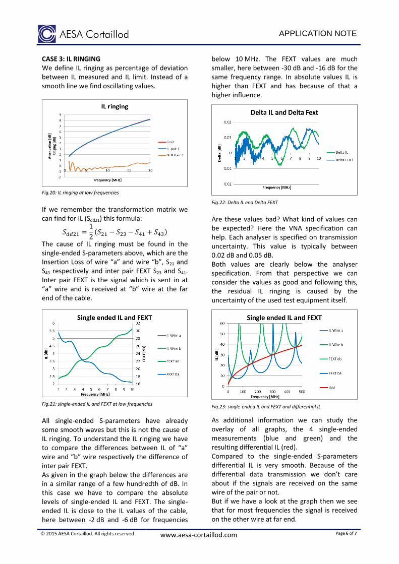
CASE 3: IL RINGING We define IL ringing as percentage of deviation between IL measured and IL limit. Instead of a smooth line we find oscillating values.
Fig.20: IL ringing at low frequencies
If we remember the transformation matrix we can find for IL (Sdd21) this formula:
𝑆𝑑𝑑21 =1
2(𝑆21 − 𝑆23 − 𝑆41 + 𝑆43)
The cause of IL ringing must be found in the single-ended S-parameters above, which are the Insertion Loss of wire “a” and wire “b”, S21 and S43 respectively and inter pair FEXT S23 and S41. Inter pair FEXT is the signal which is sent in at “a” wire and is received at “b” wire at the far end of the cable.
Fig.21: single-ended IL and FEXT at low frequencies
All single-ended S-parameters have already some smooth waves but this is not the cause of IL ringing. To understand the IL ringing we have to compare the differences between IL of “a” wire and “b” wire respectively the difference of inter pair FEXT. As given in the graph below the differences are in a similar range of a few hundredth of dB. In this case we have to compare the absolute levels of single-ended IL and FEXT. The single-ended IL is close to the IL values of the cable, here between -2 dB and -6 dB for frequencies
below 10 MHz. The FEXT values are much smaller, here between -30 dB and -16 dB for the same frequency range. In absolute values IL is higher than FEXT and has because of that a higher influence.
Fig.22: Delta IL end Delta FEXT Are these values bad? What kind of values can be expected? Here the VNA specification can help. Each analyser is specified on transmission uncertainty. This value is typically between 0.02 dB and 0.05 dB. Both values are clearly below the analyser specification. From that perspective we can consider the values as good and following this, the residual IL ringing is caused by the uncertainty of the used test equipment itself.
Fig.23: single-ended IL and FEXT and differential IL
As additional information we can study the overlay of all graphs, the 4 single-ended measurements (blue and green) and the resulting differential IL (red). Compared to the single-ended S-parameters differential IL is very smooth. Because of the differential data transmission we don’t care about if the signals are received on the same wire of the pair or not. But if we have a look at the graph then we see that for most frequencies the signal is received on the other wire at far end.

APPLICATION NOTE
© 2015 AESA Cortaillod. All rights reserved www.aesa-cortaillod.com Page 7 of 7
CONCLUSION The new opportunities as presented in this paper open a door for better understanding of data cable manufacturing and provide some insights about the way how single-ended S-parameters can be used to understand weaknesses of cables better.
Fig.24: AESA Cobalt automatic balunless measuring system.
All shown measurements in this document are
done with an AESA Cobalt system. It is fully
automated balunless test equipment which
performs all electrical tests on cables
responding to TIA°1183 and the upcoming
TIA°1183-1 to test Category 8 cables and
beyond.
Balunless testing is a great tool because it allows
accessing data from each single wire and how
they are interacting in the pair. This technology
allows analysing the cable also during
production and sorting out low performing pairs
to reduce scrap and waste of material.
In such a way of thinking it helps to reduce development cost and reaction time, check and improve the quality during each production step and improve the factory’s efficiency. Thanks to such analysis a cable manufacturer can understand and control his production better and find weak points much faster.
As proven by many papers, mathematical
superposition of single-ended S-parameters is
very accurate. Additionally to the well-known
differential S-parameters we get also mixed-
mode and common-mode S-parameters which
are based on the same single-ended
measurements but distinguished by the
algebraic signs in the formulae.
Peter Fischer, R&D Project Manager, AESA-Cortaillod
FIGURES & REFERENCES
Fig.1 IEC 61935-1
Fig.2 IEC 61156-1-2 AMD 1
Fig. 3,4,5,6,8 Fan et al (2003)
Fig.7 Fan et al (2011)
Fig.9 – 23 Measured with Cobalt
Fig.24 Cobalt balunless ATE from AESA
ABBREVIATIONS
Name Abbreviation
Cable under Test CUT
Device under Test DUT
Equal Level Transverse Conversion Transfer Loss
EL TCTL
Insertion Loss IL
Near End Crosstalk NEXT
Far End Crosstalk FEXT
Return Loss RL
Transverse Conversion Loss TCL
Vector Network Analyser VNA