Embed Size (px)
Citation preview
Balancing of Parallel U-Shaped Assembly Lines with Crossover Points
Amanpreet Rattan
Thesis submitted to the faculty of the Virginia Polytechnic Institute and State University in partial fulfillment of the requirements for the degree of
Master of Science
In
Industrial and Systems Engineering
John P. Shewchuk, Chair Manish Bansal
Ran Jin
August 11, 2017
Blacksburg, VA
Keywords: U-shaped line assembly balancing, crossover points, AMPL, Parallelization with U-shaped configuration, binary programming formulation.
Balancing of Parallel U-Shaped Assembly Lines with Crossover Points
Amanpreet Rattan
ABSTRACT
This research introduces parallel U-shaped assembly lines with crossover points. Crossover points are connecting points between two parallel U-shaped lines making the lines interdependent. The assembly lines can be employed to manufacture a variety of products belonging to the same product family. This is achieved by utilizing the concepts of crossover points, multi-line stations, and regular stations. The binary programming formulation presented in this research can be employed for any scenario (e.g. task times, cycle times, and the number of tasks) in the configuration that includes a crossover point. The comparison of numerical problem solutions based on the proposed heuristic approach with the traditional approach highlights the possible reduction in the quantity of workers required. The conclusion from this research is that a wider variety of products can be manufactured at the same capital expense using parallel U-shaped assembly lines with crossover points, leading to a reduction in the total number of workers.
Balancing of Parallel U-Shaped Assembly Lines with Crossover Points
Amanpreet Rattan
GENERAL AUDIENCE ABSTRACT
U-shaped assembly line is a production line where material moves continuously through a series of workstations/machines arranged in a U-shape. The usage of lines is for mid-volume, mid-variety production where machines are arranged based on processing sequence. There are machines on the front and back side of U-shaped line and workers are working on the layout. Raw material entering the U-shaped assembly line, and the finished product exiting the assembly line are in close proximity to improve supervision. The advantage of the U-shaped line is that one worker can work on multiple machines at the same time promoting cross functional workers. Placing two U-shaped lines in parallel can improve workstation utilization and in turn reduce the number of workstations required. This thesis aims to provide more flexibility regarding the production of a variety of products with the same product configuration. The proposed configuration permits the manufacture of new products that belong to the same product family, while using the existing machine resources.

iv
ACKNOWLEDGEMENT
This Master's thesis is the final part for my M.S. graduate degree program at Virginia Polytechnic and State University, Blacksburg, Virginia, U.S.A. The work for this research was carried out during Fall-2016, Spring-2017 and Summer-2017. I would like to thank my committee chair Dr. John Shewchuk who has supported me with critical inputs, and validated my results throughout this time frame. Without his insights, this thesis would be incomplete. Also, I would like to thank my committee members Dr. Manish Bansal and Dr. Ran Jin for their timely feedback and intuitive questions. Their inputs helped me keep my thesis on track and fulfill all the requirements.
I would like to extend my special thanks to my family and friends here in the United States and India, who have supported me and my methods of research. They have been a pillar of support throughout, and their guidance has been invaluable.
v
TABLE OF CONTENTS
ABSTRACT GENERAL AUDIENCE ABSTRACT ............................................................................................ACKNOWLEDGEMENT ............................................................................................................ ivTABLE OF CONTENTS ...............................................................................................................vLIST OF FIGURES ..................................................................................................................... viiLIST OF TABLES ..................................................................................................................... viii1. INTRODUCTION ...................................................................................................................12. PROBLEM STATEMENT ......................................................................................................43. LITERATURE REVIEW ........................................................................................................44. RESEARCH GOALS AND OBJECTIVES ............................................................................55. MATHEMATICAL MODELING AND ANALYSIS ............................................................6
5.1 Mathematical models ....................................................................................................... 65.1.1 Mathematical model for parallel U-shaped assembly line ...................................... 65.1.2 Mathematical model for parallel U-shaped assembly line
with crossover points. ........................................................................................... 105.2 Computational experiments for three small instances ................................................... 14
5.2.1 Experimental design .............................................................................................. 145.2.2 Input data .............................................................................................................. 14
5.3 Results ............................................................................................................................ 145.4 A Harder case ................................................................................................................. 17
6. HEURISTIC MODELING AND ANALYSIS ......................................................................176.1 Heuristic modeling ......................................................................................................... 176.2 Solution quality .............................................................................................................. 196.3 Numerical examples ....................................................................................................... 20
6.3.1 Input for numerical examples ............................................................................... 206.3.2 Results for numerical examples ............................................................................ 22
6.4 Comparison with the traditional approach ..................................................................... 277. DISCUSSION ........................................................................................................................298. CONCLUSIONS ...................................................................................................................29

vi
REFERENCES .............................................................................................................................31
APPENDIX A ..............................................................................................................................33
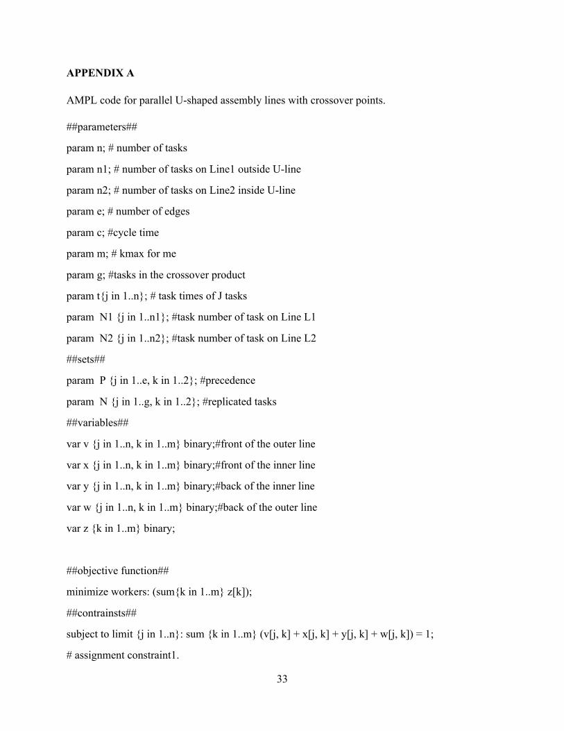
AMPL code for parallel U-shaped assembly lines with crossover points. .......................... 33
vii
LIST OF FIGURES Figure 1. Parallel U-shaped lines with crossover points. ............................................................... 2
Figure 2. Proposed configuration for products P1, P2 andP3. ..................................................... 3Figure 3. Three zones for worker placement ................................................................................. 7
Figure 4. Computational results for small instance problems. ..................................................... 16
Figure 5. Heuristic approach solution for numerical example 1. ................................................. 22
Figure 6. Heuristic approach solution for numerical example 2. ................................................. 23Figure 7. Heuristic approach solution for numerical example 3. ................................................. 24
Figure 8. Heuristic approach solution for numerical example 4. ................................................. 25
Figure 9. Line occupancy and scheduling display for numerical example 4 ............................... 26
viii
LIST OF TABLES Table 1. Input data for four small instance problems. ............................................................... 15Table 2. Solution quality when comparing the optimal value and the heuristic value. ............. 20Table 3. Input data for industrial grade numerical examples ..................................................... 21Table 4. Comparative results between the traditional approach and the
proposed heuristic approach ....................................................................................... 27
1
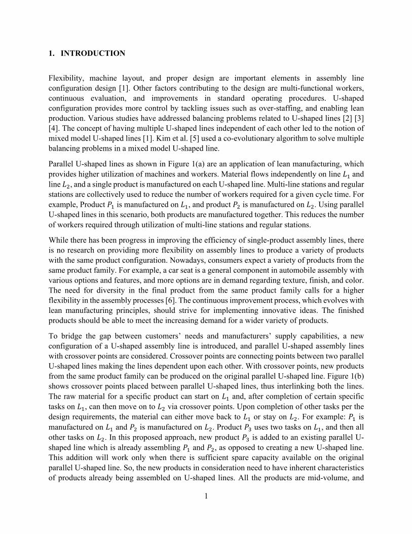
1. INTRODUCTION
Flexibility, machine layout, and proper design are important elements in assembly line configuration design [1]. Other factors contributing to the design are multi-functional workers, continuous evaluation, and improvements in standard operating procedures. U-shaped configuration provides more control by tackling issues such as over-staffing, and enabling lean production. Various studies have addressed balancing problems related to U-shaped lines [2] [3] [4]. The concept of having multiple U-shaped lines independent of each other led to the notion of mixed model U-shaped lines [1]. Kim et al. [5] used a co-evolutionary algorithm to solve multiple balancing problems in a mixed model U-shaped line.
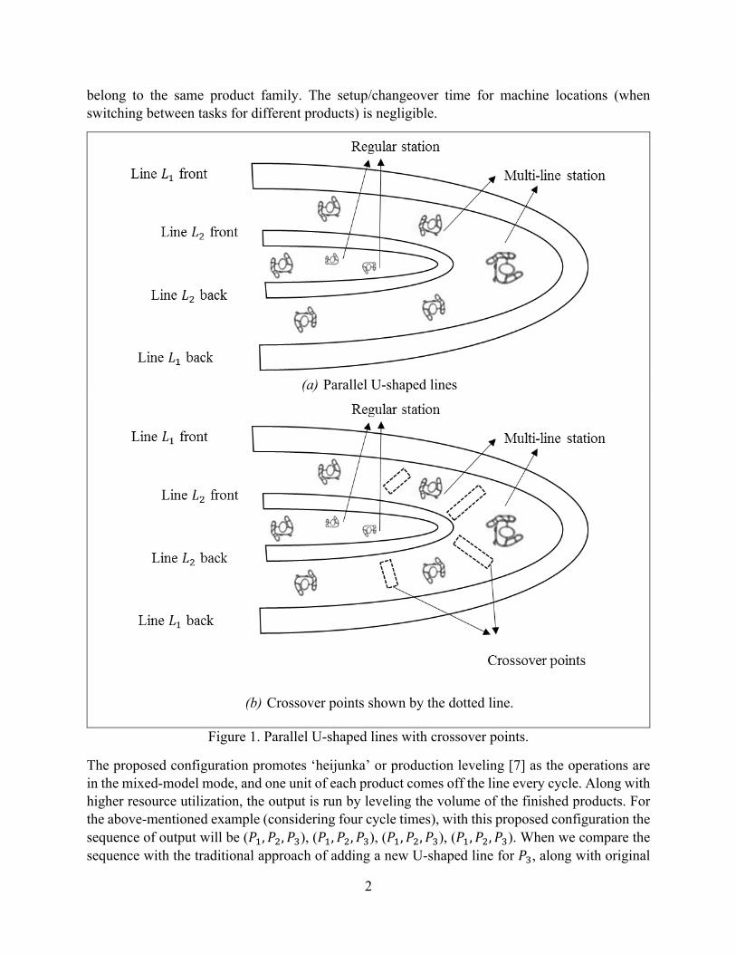
Parallel U-shaped lines as shown in Figure 1(a) are an application of lean manufacturing, which provides higher utilization of machines and workers. Material flows independently on line 𝐿'and line 𝐿(, and a single product is manufactured on each U-shaped line. Multi-line stations and regular stations are collectively used to reduce the number of workers required for a given cycle time. For example, Product 𝑃' is manufactured on 𝐿', and product 𝑃( is manufactured on 𝐿(. Using parallel U-shaped lines in this scenario, both products are manufactured together. This reduces the number of workers required through utilization of multi-line stations and regular stations. While there has been progress in improving the efficiency of single-product assembly lines, there is no research on providing more flexibility on assembly lines to produce a variety of products with the same product configuration. Nowadays, consumers expect a variety of products from the same product family. For example, a car seat is a general component in automobile assembly with various options and features, and more options are in demand regarding texture, finish, and color. The need for diversity in the final product from the same product family calls for a higher flexibility in the assembly processes [6]. The continuous improvement process, which evolves with lean manufacturing principles, should strive for implementing innovative ideas. The finished products should be able to meet the increasing demand for a wider variety of products.
To bridge the gap between customers’ needs and manufacturers’ supply capabilities, a new configuration of a U-shaped assembly line is introduced, and parallel U-shaped assembly lines with crossover points are considered. Crossover points are connecting points between two parallel U-shaped lines making the lines dependent upon each other. With crossover points, new products from the same product family can be produced on the original parallel U-shaped line. Figure 1(b) shows crossover points placed between parallel U-shaped lines, thus interlinking both the lines. The raw material for a specific product can start on 𝐿' and, after completion of certain specific tasks on 𝐿', can then move on to 𝐿( via crossover points. Upon completion of other tasks per the design requirements, the material can either move back to 𝐿' or stay on 𝐿(. For example: 𝑃' is manufactured on 𝐿' and 𝑃( is manufactured on 𝐿(. Product 𝑃* uses two tasks on 𝐿', and then all other tasks on 𝐿(. In this proposed approach, new product 𝑃* is added to an existing parallel U-shaped line which is already assembling 𝑃' and 𝑃(, as opposed to creating a new U-shaped line. This addition will work only when there is sufficient spare capacity available on the original parallel U-shaped line. So, the new products in consideration need to have inherent characteristics of products already being assembled on U-shaped lines. All the products are mid-volume, and
2
belong to the same product family. The setup/changeover time for machine locations (when switching between tasks for different products) is negligible.
(a) Parallel U-shaped lines
(b) Crossover points shown by the dotted line.
Figure 1. Parallel U-shaped lines with crossover points.
The proposed configuration promotes ‘heijunka’ or production leveling [7] as the operations are in the mixed-model mode, and one unit of each product comes off the line every cycle. Along with higher resource utilization, the output is run by leveling the volume of the finished products. For the above-mentioned example (considering four cycle times), with this proposed configuration the sequence of output will be (𝑃', 𝑃(, 𝑃*), (𝑃', 𝑃(, 𝑃*), (𝑃', 𝑃(, 𝑃*), (𝑃', 𝑃(, 𝑃*). When we compare the sequence with the traditional approach of adding a new U-shaped line for 𝑃*, along with original

3
parallel U-shaped line for 𝑃'and 𝑃(, the sequence of outputs for four cycle times, is (𝑃', 𝑃(), 𝑃* , (𝑃', 𝑃(), 𝑃* . The above sequence signifies the possible improvements using this proposed configuration.
Parallel U-shaped lines with crossover points enable manufacturing of all three products at the same time. This leads to a reduction in the total quantity of workers required by utilizing crossover points, multi-line stations, and regular stations. This configuration combines the advantages of parallel assembly lines [8] with the U-shaped assembly lines [9], and adds crossover points. The introduction of crossover points enables material flow on either of the U-shaped lines. This permits the manufacture of new products that belong to the same product family, and use the same machine resources. U-shaped lines are dependent, and tasks must be scheduled in such a way, that no previous task for a specific product is being processed when the next task for a different product arrives on same machine/task location. The nature of the problem, and the need for crossover points, are illustrated using an example problem.
The U-shaped assembly line configuration in this problem manufactures three products 𝑃', 𝑃(, and 𝑃*, as shown in Figure 2. Products 𝑃' and 𝑃( are assembled on original parallel U-shaped line. Takt time (cycle time) was determined based on demand and planning horizons, and defined as the average time for production, divided by required quantity of products.
Figure 2. Proposed configuration for products P', P( andP*.
New product 𝑃* is introduced which is of the same product family as𝑃'and𝑃(, and needs the same capital machines. 𝑃* can be assembled using linear lines or a new U-shaped line. Previous research has established that using a U-shaped line instead of a linear line is economical [9]. In the present scenario, we need to lay down one more U-shaped line to start production of 𝑃*. With the proposed configuration (by adding a crossover point on the assembly line) the production of 𝑃*
Task1 Task2
Task3
Task4Task5
Task6
Task7
Task8
Input/source
Output/sink
Product 𝑃*, assembly on dotted line.

4
can be done without laying down any new assembly line. In Figure 2, after deciding the key crossover points in the parallel U-shaped line, 𝑃* is manufactured. 𝑃* will need tasks 9, 10, 11, 12, and 13 in that sequence, where tasks 9, 10, 11, 12, and 13 are done at the same locations as tasks 1, 2, 7, 4, and 5 respectively. Using crossover points will allow the material to flow from 𝐿' to 𝐿( and back as required. 𝑃'and𝑃( are assembled on the original set of parallel U-shaped lines shown as solid line. 𝑃* follows the dotted line.
The rest of the thesis is organized as follows. In Chapter 2, the problem statement is defined, followed by literature review in Chapter 3. Research goals and objectives are established in Chapter 4. In Chapter 5, mathematical models are developed, and these models are verified using three small instance examples. Chapter 6 introduces the heuristic modeling and analysis, followed by four relatively large size numerical examples, and the corresponding results. Discussion of the results and overall advantages of this proposed configuration are presented in Chapter 7. Chapter 8 concludes the thesis and includes future work.
2. PROBLEM STATEMENT This research proposes a parallel U-shaped line configuration that incorporates crossover points. The configuration can be employed to manufacture a higher variety of products using the same capital machines. As crossover points are integrated, the U-shaped lines are no longer independent. Material moving from one line to the next line may have to wait because another material is already on that same machine at the same time. These scheduling delays must be accounted for while assigning tasks to the workstations. One worker occupies each workstation. The total manual time per workstation must be less than or equal to the cycle time, and should also include material (task) waiting time. The research addresses assembly line balancing for parallel U-shaped assembly lines that include crossover points.
3. LITERATURE REVIEW Miltenburg and Wijngaard [9] studied U-shaped assembly line balancing, and Urban [2] developed a model of U-line involving a single product using an integer programming approach. However, the proposed configuration investigates multiple products on a parallel U-shaped line setup. Korkmazel and Meral [10] introduced mixed-model assembly lines as efficient means to manufacture various models in batch sizes on a single line. Although multiple products were in discussion, only a single line was considered. Miltenburg [11] described benefits of the simple U-shaped line over the traditional linear line with the help of case studies and examples.
Kim et al. [5] found that a significant advantage of U-shaped lines over linear lines is that precedence restriction is relaxed in the former. The available tasks on a U-shaped line are a set of tasks whose predecessors have been completed and whose successors are already assigned. This research will employ this precedence restriction relaxation in determining the available task list (ATL) for each U-shaped line. Shewchuk [12] utilized the concept of circular walking paths where the performance of a U-shaped line is improved when workers walk around one another. The
5
proposed configuration emphasizes maximizing full work and minimizing the quantity of workers. Full work is defined as the average of utilization of all workstations, except the least utilized workstation. The workstation utilization is defined as the sum of all allocated tasks to a workstation, divided by the cycle time. The general range for high utilized workstation in a manufacturing environment is 85-90%. The least utilized workstation is defined as a workstation which has a single task assigned to it, and the workstation utilization is less than 40%. U-shaped lines have numerous practical applications in industry [13] [14] [15].
Gokcen et al. [8] proposed a parallel line system. Subsequent research has successfully hybridized this concept. Ozcan et al. [16], and Kucukkoc and Zhang [17] [18] researched parallel mixed-model lines, and two-sided parallel mixed-model lines. These research studies presented advantages of parallel two-sided lines and mixed-model parallel two-sided lines.
Multiple U-shaped lines balancing techniques were introduced by Chiang et al. [19]. They considered multiple U-shaped lines in a Just-in-time (J.I.T) production system. Comparing Chiang et al. [19] to Miltenburg et al. [1], the difference is the consideration of multiple U-shaped lines which were independent of each other. In the proposed configuration, the parallel U-shaped lines are dependent upon each other. Shewchuk [20] discussed the overlap in the tasks’ timing for the utilization of helper tasks. The proposed configuration ensures that there is no overlap between the tasks scheduled on each U-shaped line.
Kucukkoc and Zhang [21] proposed a parallel configuration of U-shaped assembly lines. The advantage of this configuration is the flexibility in terms of workstation utilization. Introducing parallelization with U-shaped configuration increases the worker utilization in a significant manner. However, in this research, both the U-shaped lines were independent and there were no crossover points connecting both the U-shaped lines. With the introduction of crossover points, the material can flow from one U-shaped line to another U-shaped line making them interdependent.
The concept of parallel U-shaped assembly lines with crossover points offers many opportunities regarding improving flexibility in terms of workstation utilization. There is no literature available in the line balancing of dependent U-shaped lines which include crossover points. This literature review contextualizes the need for the proposed configuration to bridge the gap between the existing literature, and customer expectation for a variety of products in the same product family.
4. RESEARCH GOALS AND OBJECTIVES The goal of this research is to investigate the potential of using parallel U-shaped assembly lines with crossover points. This research introduces the concept of employing crossover points in parallel U-shaped assembly lines. There is no existing literature for the proposed configuration.
The main objective of this research is to model the problem of balancing the parallel U-shaped assembly lines with crossover points mathematically, where an intent to minimize the quantity of workers. The second objective is to validate the mathematical model by employing a
6
commercially-available optimization software package. If the line balancing problem becomes intractable, a heuristic technique will be developed. The last objective is to perform a comparative analysis to determine the quality of the heuristic solution.
5. MATHEMATICAL MODELING AND ANALYSIS
A mathematical model for parallel U-shaped lines is developed and validated. The model is then upgraded for parallel U-shaped lines with crossover points. The models assume that different products are manufactured in the same quantity. So, if we manufacture three products - 𝑃', 𝑃(, and 𝑃* - each product exits the line identically.
The assumptions are:
• Production characteristics are the same for different product models. • The product uses a finite number of workstations. • Precedence diagram of all product models is known. • Task completion time is deterministic and independent of the assigned workstation. • The workers’ travel times are ignored. • The presence of common tasks between product models makes this configuration possible. • The completion time may be different for different models on each workstation. • The completion time for a product task on any workstation can be zero. • Setup times and changeover times for machines are negligible and ignored.
5.1 Mathematical models
Kucukkoc and Zhang [21] proposed parallel U-shaped assembly line configuration, and the associated mathematical model was proposed as future research extension.
5.1.1 Mathematical model for parallel U-shaped assembly line
Assumption: (i) Two products 𝑃' and 𝑃( only.
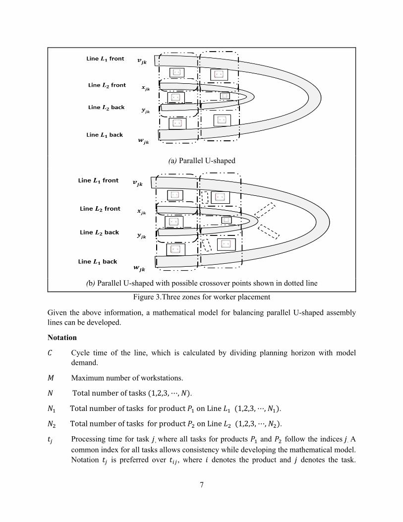
As shown in Figure 3(a), a parallel U-shaped assembly line configuration is considered, and two products (𝑃' and 𝑃() are being manufactured on this assembly line. 𝑃' is manufactured on 𝐿', [outer U-shaped line in Figure 3(a)] and 𝑃( on 𝐿( [inner U-shaped line in Figure 3(a)]. 𝑷 is the precedence for the tasks 𝑖, 𝑗; where (𝑖, 𝑗) ∈ 𝑁, and 𝐸 is the number of edges in the tuple dimension of 𝑷. For example, in a 𝑷 tuple for 5 tasks (1,2,3,4,5), the value of 𝐸 is 4 [(1,3), (2,3), (3,4), (4,5)].
7
(a) Parallel U-shaped
(b) Parallel U-shaped with possible crossover points shown in dotted line
Figure 3.Three zones for worker placement
Given the above information, a mathematical model for balancing parallel U-shaped assembly lines can be developed.
Notation
𝐶 Cycle time of the line, which is calculated by dividing planning horizon with model demand.
𝑀 Maximum number of workstations.
𝑁Totalnumberoftasks(1,2,3,⋯,𝑁).
𝑁'Totalnumberoftasksforproduct𝑃'onLine𝐿'(1,2,3,⋯,𝑁').
𝑁(Totalnumberoftasksforproduct𝑃(onLine𝐿((1,2,3,⋯,𝑁().
𝑡K Processing time for task 𝑗, where all tasks for products 𝑃' and 𝑃( follow the indices𝑗. A common index for all tasks allows consistency while developing the mathematical model. Notation 𝑡K is preferred over 𝑡LK, where 𝑖 denotes the product and 𝑗 denotes the task.

8
Ignoring 𝑖 for product, and generalizing all the tasks collectively, makes the mathematical model more compatible with the proposed configuration.
𝑷 𝑖, 𝑗 : 𝑡𝑎𝑠𝑘𝑖𝑝𝑟𝑒𝑐𝑒𝑑𝑒𝑠𝑡𝑎𝑠𝑘𝑗 , 𝑖 ∈ 1,⋯ ,𝑁 , 𝑗 ∈ 1,⋯ ,𝑁
where 𝑃 is a known forward and backward precedence for all the models.
𝑃VWX Total number of products manufactured on the assembly lines.
𝐸 Number of edges in the graphical representation of 𝑷 when connecting all the nodes in the precedence 𝑷.
Indices:
𝑘 Number of workstations (1,2,3,⋯ ,𝑀)
𝑗 Task number (1,2,3,⋯ ,𝑁)
Decision variables
𝑣K[ =1,iftask𝑗,assignedtoworkstation𝑘,ontheU-Shapedline𝐿'front.=0,otherwise
𝑥K[ =1,iftask𝑗,assignedtoworkstation𝑘,ontheU-Shapedline𝐿(front.=0,otherwise
𝑦K[ =1,iftask𝑗,assignedtoworkstation𝑘,ontheU-Shapedline𝐿(back.=0,otherwise
𝑤K[ =1,iftask𝑗,assignedtoworkstation𝑘,ontheU-Shapedline𝐿'back.=0,otherwise
𝑧[ =1,ifstation𝑘isused.
=0,otherwise
Using the above notations, the mathematical model can be expressed as follows:
𝑚𝑖𝑛 𝑧[
j
[k'
(1)
Subject to Assignment constraints:
(𝑣K[ +𝑥K[ +𝑦K[ + 𝑤K[)j
[k'
= 1, 𝑗 = 1,⋯ ,𝑁 (2)
9
Capacity constraints for each workstation per the cycle time:
𝑣K[ +𝑥K[ +𝑦K[ + 𝑤K[ 𝑡K ≤n
Kk'
𝐶 ∙ 𝑧[, 𝑘 = 1,⋯ ,𝑀 (3)
Precedence constraints: Forward precedence constraints for 𝑣:
𝑀 − 𝑘 + 1 𝑣L[ − 𝑣K[} ≥ 0,j
[k'
𝑖 = 1,⋯ , 𝐸; 𝑗 = 1,⋯ , 𝐸 (4)
Forward precedence constraints for 𝑥:
𝑀 − 𝑘 + 1 𝑥L[ − 𝑥K[} ≥ 0,j
[k'
𝑖 = 1,⋯ , 𝐸; 𝑗 = 1,⋯ , 𝐸 (5)
Backward precedence constraints for 𝑦:
𝑀 − 𝑘 + 1 𝑦K[ − 𝑦L[} ≥ 0,j
[k'
𝑖 = 1,⋯ , 𝐸; 𝑗 = 1,⋯ , 𝐸 (6)
Backward precedence constraints for 𝑤:
𝑀 − 𝑘 + 1 𝑤K[ − 𝑤L[} ≥ 0,j
[k'
𝑖 = 1,⋯ , 𝐸; 𝑗 = 1,⋯ , 𝐸 (7)
Positional constraints: Positional constraints 1: 𝑤L[ +𝑥K[ = 1,𝑘 = 1,⋯ ,𝑀; 𝑖 = 1,⋯ ,𝑁; 𝑗 = 1,⋯ ,𝑁; 𝑖 ≠ 𝑗 (8)
Positional constraints 2: 𝑤L[ +𝑣K[ = 1,𝑘 = 1,⋯ ,𝑀; 𝑖 = 1,⋯ ,𝑁; 𝑗 = 1,⋯ ,𝑁; 𝑖 ≠ 𝑗 (9)
Positional constraints 3: 𝑦L[ +𝑣K[ = 1,𝑘 = 1,⋯ ,𝑀; 𝑖 = 1,⋯ ,𝑁; 𝑗 = 1,⋯ ,𝑁; 𝑖 ≠ 𝑗 (10)
Product task placement constraints for 𝑳𝟏: Product task placement constraints 1:
𝑥K[ +𝑦K[ = 0K∈𝑵𝟏
, 𝑘 = 1,⋯ ,𝑀 (11)
Product task placement constraints for 𝑳𝟐: Product task placement constraints 2:
𝑣K[ +𝑤K[ = 0K∈𝑵𝟐
, 𝑘 = 1,⋯ ,𝑀 (12)
10
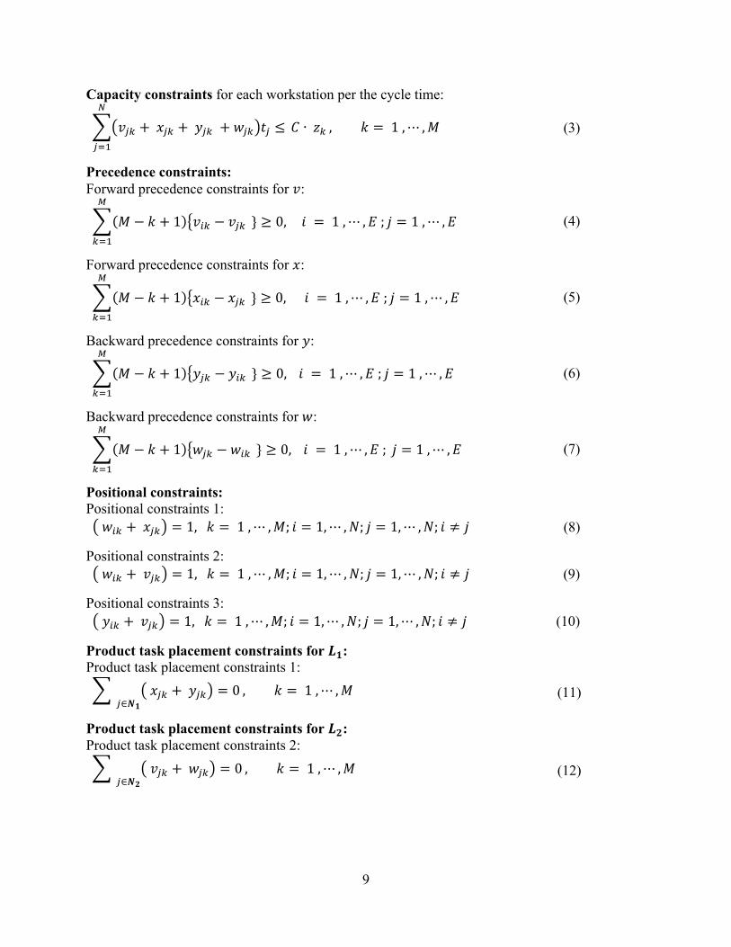
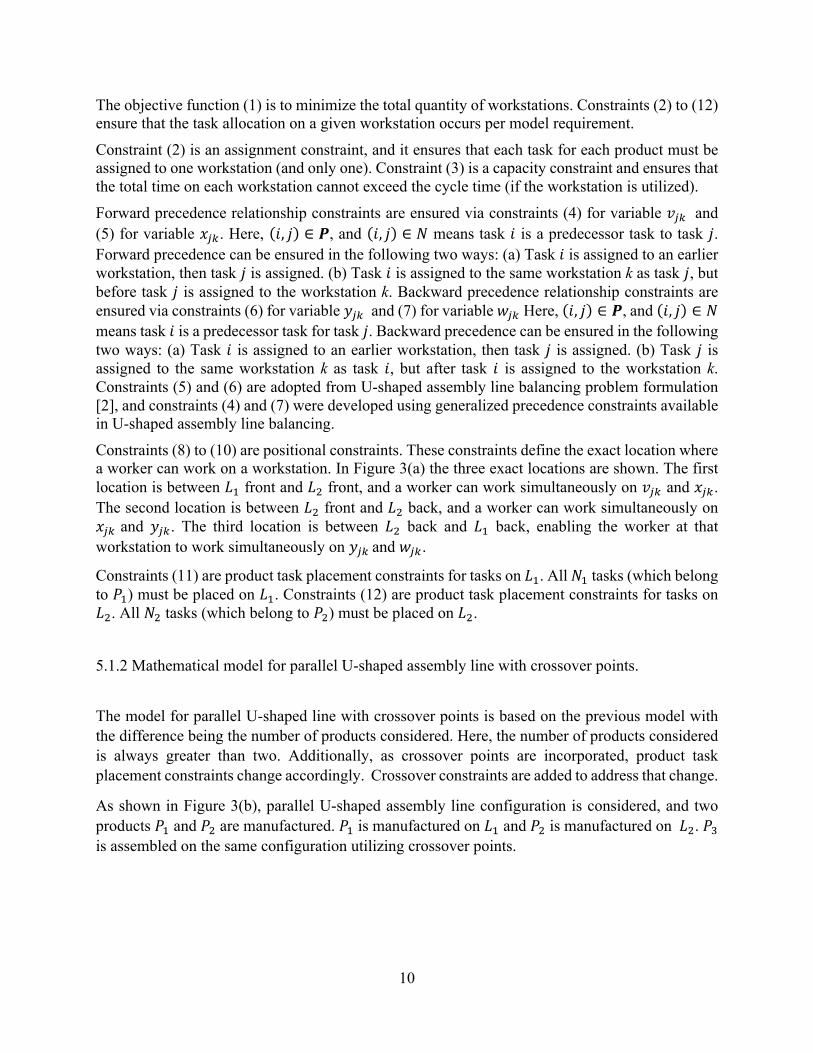
The objective function (1) is to minimize the total quantity of workstations. Constraints (2) to (12) ensure that the task allocation on a given workstation occurs per model requirement.
Constraint (2) is an assignment constraint, and it ensures that each task for each product must be assigned to one workstation (and only one). Constraint (3) is a capacity constraint and ensures that the total time on each workstation cannot exceed the cycle time (if the workstation is utilized).
Forward precedence relationship constraints are ensured via constraints (4) for variable 𝑣K[ and (5) for variable 𝑥K[. Here, 𝑖, 𝑗 ∈ 𝑷, and 𝑖, 𝑗 ∈ 𝑁 means task 𝑖 is a predecessor task to task 𝑗. Forward precedence can be ensured in the following two ways: (a) Task 𝑖 is assigned to an earlier workstation, then task 𝑗 is assigned. (b) Task 𝑖 is assigned to the same workstation k as task 𝑗, but before task 𝑗 is assigned to the workstation k. Backward precedence relationship constraints are ensured via constraints (6) for variable 𝑦K[ and (7) for variable 𝑤K[ Here, 𝑖, 𝑗 ∈ 𝑷, and 𝑖, 𝑗 ∈ 𝑁 means task 𝑖 is a predecessor task for task 𝑗. Backward precedence can be ensured in the following two ways: (a) Task 𝑖 is assigned to an earlier workstation, then task 𝑗 is assigned. (b) Task 𝑗 is assigned to the same workstation k as task 𝑖, but after task 𝑖 is assigned to the workstation k. Constraints (5) and (6) are adopted from U-shaped assembly line balancing problem formulation [2], and constraints (4) and (7) were developed using generalized precedence constraints available in U-shaped assembly line balancing.
Constraints (8) to (10) are positional constraints. These constraints define the exact location where a worker can work on a workstation. In Figure 3(a) the three exact locations are shown. The first location is between 𝐿' front and 𝐿( front, and a worker can work simultaneously on 𝑣K[ and 𝑥K[. The second location is between 𝐿( front and 𝐿( back, and a worker can work simultaneously on 𝑥K[ and 𝑦K[. The third location is between 𝐿( back and 𝐿' back, enabling the worker at that workstation to work simultaneously on 𝑦K[ and 𝑤K[.
Constraints (11) are product task placement constraints for tasks on 𝐿'. All 𝑁' tasks (which belong to 𝑃') must be placed on 𝐿'. Constraints (12) are product task placement constraints for tasks on 𝐿(. All 𝑁( tasks (which belong to 𝑃() must be placed on 𝐿(.
5.1.2 Mathematical model for parallel U-shaped assembly line with crossover points.
The model for parallel U-shaped line with crossover points is based on the previous model with the difference being the number of products considered. Here, the number of products considered is always greater than two. Additionally, as crossover points are incorporated, product task placement constraints change accordingly. Crossover constraints are added to address that change.
As shown in Figure 3(b), parallel U-shaped assembly line configuration is considered, and two products 𝑃' and 𝑃( are manufactured. 𝑃' is manufactured on 𝐿' and 𝑃( is manufactured on 𝐿(. 𝑃* is assembled on the same configuration utilizing crossover points.

11
Notation
𝐶 Cycle time of the line, which is calculated by dividing planning horizon with model demand.
𝑀 Maximum number of workstations.
𝑁Totalnumberoftasks(1,2,3,⋯,𝑁)
𝑁'Totalnumberoftasksforproduct𝑃'andproduct𝑃*onLine𝐿'(1,2,3,⋯,𝑁')
𝑁(Totalnumberoftasksforproduct𝑃(andproduct𝑃*onLine𝐿((1,2,3,⋯,𝑁()
𝑡K Processing time for task 𝑗
𝑷 𝑖, 𝑗 : 𝑡𝑎𝑠𝑘𝑖𝑝𝑟𝑒𝑐𝑒𝑑𝑒𝑠𝑡𝑎𝑠𝑘𝑗 , 𝑖 ∈ 1,⋯ ,𝑁 , 𝑗 ∈ 1,⋯ ,𝑁
where 𝑃 is a known forward and backward precedence for all the models.
𝑃VWX Total number of products manufactured on the assembly lines.
𝐸 Number of edges in the graphical representation of 𝑷 when connecting all the nodes in the precedence 𝑷.
𝐺 Number of tasks for the product using crossover points. (Replicated task)
𝛾 Matrix of dimension 𝐺𝑋2 , associating the parent task and physical replicated task.
Indices:
𝑘 Number of workstations (1,2,3,⋯ ,𝑀)
𝑗 Task number (1,2,3,⋯ ,𝑁)
Decision variables
𝑣K[ =1,iftask𝑗,assignedtoworkstation𝑘,ontheU-Shapedline𝐿'front.=0,otherwise
𝑥K[ =1,iftask𝑗,assignedtoworkstation𝑘,ontheU-Shapedline𝐿(front.=0,otherwise
𝑦K[ =1,iftask𝑗,assignedtoworkstation𝑘,ontheU-Shapedline𝐿(back.=0,otherwise
𝑤K[ =1,iftask𝑗,assignedtoworkstation𝑘,ontheU-Shapedline𝐿'back.=0,otherwise
𝑧[ =1,ifstation𝑘isused.
=0,otherwise
Using the above notations, the mathematical model can be expressed as follows:
12
𝑚𝑖𝑛 𝑧[
j
[k'
(1)
Subject to Assignment constraints:
(𝑣K[ +𝑥K[ +𝑦K[ + 𝑤K[)j
[k'
= 1, 𝑗 = 1,⋯ ,𝑁 (2)
Capacity constraints for each workstation per the cycle time:
𝑣K[ +𝑥K[ +𝑦K[ + 𝑤K[ 𝑡K ≤n
Kk'
𝐶 ∙ 𝑧[, 𝑘 = 1,⋯ ,𝑀 (3)
Precedence constraints: Forward precedence constraints for 𝑣:
𝑀 − 𝑘 + 1 𝑣L[ − 𝑣K[} ≥ 0,j
[k'
𝑖 = 1,⋯ , 𝐸; 𝑗 = 1,⋯ , 𝐸 (4)
Forward precedence constraints for 𝑥:
𝑀 − 𝑘 + 1 𝑥L[ − 𝑥K[} ≥ 0,j
[k'
𝑖 = 1,⋯ , 𝐸; 𝑗 = 1,⋯ , 𝐸 (5)
Backward precedence constraints for 𝑦:
𝑀 − 𝑘 + 1 𝑦K[ − 𝑦L[} ≥ 0,j
[k'
𝑖 = 1,⋯ , 𝐸; 𝑗 = 1,⋯ , 𝐸 (6)
Backward precedence constraints for 𝑤:
𝑀 − 𝑘 + 1 𝑤K[ − 𝑤L[} ≥ 0,j
[k'
𝑖 = 1,⋯ , 𝐸; 𝑗 = 1,⋯ , 𝐸 (7)
Positional constraints: Positional constraints 1: 𝑤L[ +𝑥K[ = 1,𝑘 = 1,⋯ ,𝑀; 𝑖 = 1,⋯ ,𝑁; 𝑗 = 1,⋯ ,𝑁; 𝑖 ≠ 𝑗 (8)
Positional constraints 2: 𝑤L[ +𝑣K[ = 1,𝑘 = 1,⋯ ,𝑀; 𝑖 = 1,⋯ ,𝑁; 𝑗 = 1,⋯ ,𝑁; 𝑖 ≠ 𝑗 (9)
Positional constraints 3: 𝑦L[ +𝑣K[ = 1,𝑘 = 1,⋯ ,𝑀; 𝑖 = 1,⋯ ,𝑁; 𝑗 = 1,⋯ ,𝑁; 𝑖 ≠ 𝑗 (10)
13
Product task placement constraints for 𝑳𝟏: Product task placement constraints 1 for P1 and P3:
𝑥K[ +𝑦K[ = 0K∈𝑵𝟏
, 𝑘 = 1,⋯ ,𝑀 (11)
Product task placement constraints for 𝑳𝟐: Product task placement constraints 2 for P2 and P3:
𝑣K[ +𝑤K[ = 0K∈𝑵𝟐
, 𝑘 = 1,⋯ ,𝑀 (12)
Crossover constraints:
(𝑥| L,' ,[ −𝑥| L,( ,[)j
[k'
≤ 0,𝑖 = 1,⋯ , 𝐺 (13)
(𝑥| L,( ,[ −𝑥| L,' ,[)j
[k'
≤ 0,𝑖 = 1,⋯ , 𝐺 (14)
(𝑦| L,' ,[ −𝑦| L,( ,[)j
[k'
≤ 0,𝑖 = 1,⋯ , 𝐺 (15)
(𝑦| L,( ,[ −𝑦| L,' ,[)j
[k'
≤ 0,𝑖 = 1,⋯ , 𝐺 (16)
(𝑣| L,' ,[ −𝑣| L,( ,[)j
[k'
≤ 0,𝑖 = 1,⋯ , 𝐺 (17)
(𝑣| L,( ,[ −𝑣| L,' ,[)j
[k'
≤ 0,𝑖 = 1,⋯ , 𝐺 (18)
(𝑤| L,' ,[ −𝑤| L,( ,[)j
[k'
≤ 0,𝑖 = 1,⋯ , 𝐺 (19)
(𝑤| L,( ,[ −𝑤| L,' ,[)j
[k'
≤ 0,𝑖 = 1,⋯ , 𝐺 (20)
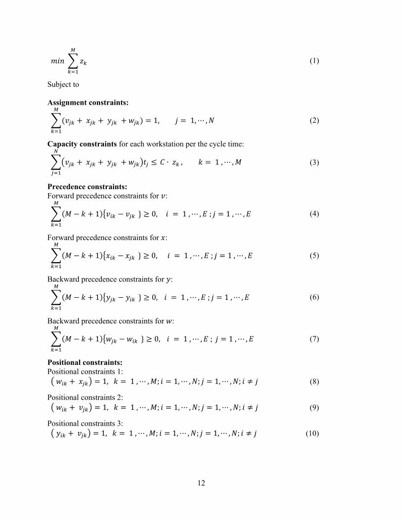
The objective function (1) is to minimize the total quantity of workstations. Constraints (2) to (12) ensure that task allocation on a workstation occurs per model requirement. Constraints (2) to (10) work as described in the previous section for the mathematical model for parallel U-shaped lines. In Figure 3(b) the three exact work locations are shown based on constraints (8), (9), and (10). Constraint (11) is product task placement constraint for tasks on 𝐿'. All 𝑁'tasks (which belong to 𝑃'and𝑃*) must be placed on Line 𝐿'. Constraint (12) is product task placement constraint for tasks on 𝐿(. All 𝑁(tasks (which belong to 𝑃(and𝑃*) must be placed on 𝐿(.
14
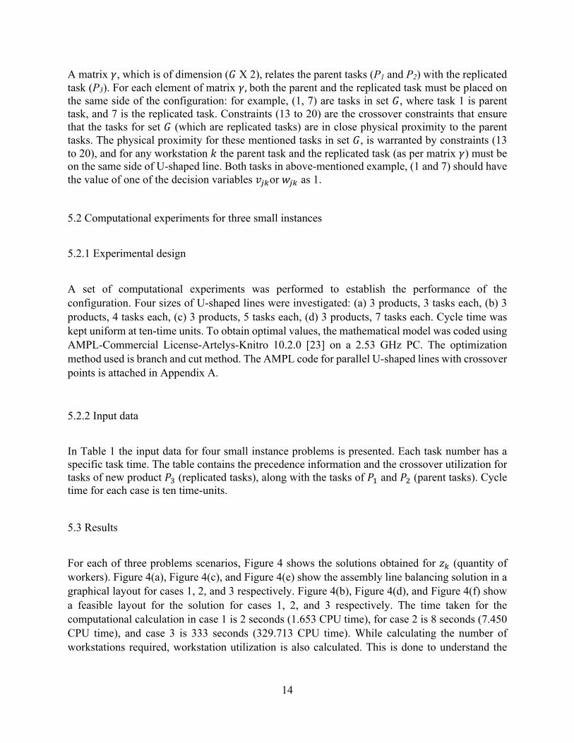
A matrix 𝛾, which is of dimension (𝐺 X 2), relates the parent tasks (P1 and P2) with the replicated task (P3). For each element of matrix 𝛾,both the parent and the replicated task must be placed on the same side of the configuration: for example, (1, 7) are tasks in set 𝐺, where task 1 is parent task, and 7 is the replicated task. Constraints (13 to 20) are the crossover constraints that ensure that the tasks for set 𝐺 (which are replicated tasks) are in close physical proximity to the parent tasks. The physical proximity for these mentioned tasks in set 𝐺, is warranted by constraints (13 to 20), and for any workstation 𝑘 the parent task and the replicated task (as per matrix 𝛾) must be on the same side of U-shaped line. Both tasks in above-mentioned example, (1 and 7) should have the value of one of the decision variables 𝑣K[or 𝑤K[ as 1.
5.2 Computational experiments for three small instances
5.2.1 Experimental design
A set of computational experiments was performed to establish the performance of the configuration. Four sizes of U-shaped lines were investigated: (a) 3 products, 3 tasks each, (b) 3 products, 4 tasks each, (c) 3 products, 5 tasks each, (d) 3 products, 7 tasks each. Cycle time was kept uniform at ten-time units. To obtain optimal values, the mathematical model was coded using AMPL-Commercial License-Artelys-Knitro 10.2.0 [23] on a 2.53 GHz PC. The optimization method used is branch and cut method. The AMPL code for parallel U-shaped lines with crossover points is attached in Appendix A.
5.2.2 Input data
In Table 1 the input data for four small instance problems is presented. Each task number has a specific task time. The table contains the precedence information and the crossover utilization for tasks of new product 𝑃* (replicated tasks), along with the tasks of 𝑃' and 𝑃( (parent tasks). Cycle time for each case is ten time-units.
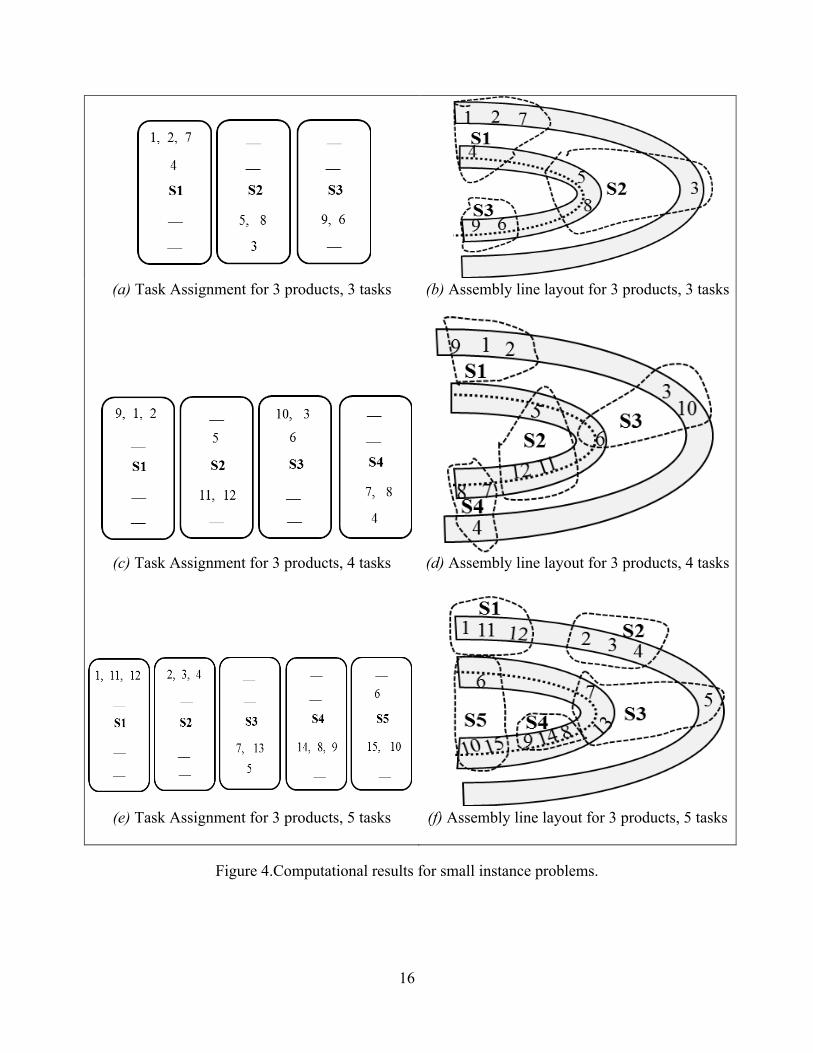
5.3 Results
For each of three problems scenarios, Figure 4 shows the solutions obtained for 𝑧[(quantity of workers). Figure 4(a), Figure 4(c), and Figure 4(e) show the assembly line balancing solution in a graphical layout for cases 1, 2, and 3 respectively. Figure 4(b), Figure 4(d), and Figure 4(f) show a feasible layout for the solution for cases 1, 2, and 3 respectively. The time taken for the computational calculation in case 1 is 2 seconds (1.653 CPU time), for case 2 is 8 seconds (7.450 CPU time), and case 3 is 333 seconds (329.713 CPU time). While calculating the number of workstations required, workstation utilization is also calculated. This is done to understand the
15
concept of full work; and with an implicit goal to clearly mark stations with improvement possibilities.
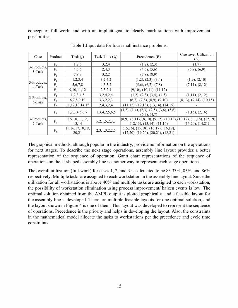
Table 1.Input data for four small instance problems.
Case Product Task (𝑗) Task Time (𝑡K) Precedence (𝑷) Crossover Utilization (𝐺)
3-Products, 3-Task
𝑃' 1,2,3 3,2,4 (1,2), (2,3) (1,7) 𝑃( 4,5,6 2,4,3 (4,5), (5,6) (5,8), (6,9) 𝑃* 7,8,9 3,2,2 (7,8), (8,9) -
3-Products, 4-Task
𝑃' 1,2,3,4 3,2,4,2 (1,2), (2,3), (3,4) (1,9), (2,10) 𝑃( 5,6,7,8 4,3,3,2 (5,6), (6,7), (7,8) (7,11), (8,12) 𝑃* 9,10,11,12 2,3,2,4 (9,10), (10,11), (11,12) -
3-Products, 5-Task
𝑃' 1,2,3,4,5 3,2,4,2,4 (1,2), (2,3), (3,4), (4,5) (1,11), (2,12) 𝑃( 6,7,8,9,10 3,3,2,2,3 (6,7), (7,8), (8,9), (9,10) (8,13), (9,14), (10,15) 𝑃* 11,12,13,14,15 2,4,3,2,4 (11,12), (12,13), (13,14), (14,15) -
3-Products, 7-Task
𝑃' 1,2,3,4,5,6,7 1,3,4,2,5,6,5 (1,2), (1,4), (2,3), (2,5), (3,6), (5,6), (6,7), (4,7) (1,15), (2,16)
𝑃( 8,9,10,11,12, 13,14 5,2,1,5,2,3,3 (8,9), (8,11), (8,10), (9,12), (10,13),
(12,13), (13,14), (11,14) (10,17), (11,18), (12,19),
(13,20), (14,21)
𝑃* 15,16,17,18,19, 20,21 2,3,1,3,2,2,5 (15,16), (15,18), (16,17), (16,19),
(17,20), (19,20), (20,21), (18,21) -
The graphical methods, although popular in the industry, provide no information on the operations for next stages. To describe the next stage operations, assembly line layout provides a better representation of the sequence of operation. Gantt chart representations of the sequence of operations on the U-shaped assembly line is another way to represent each stage operations.
The overall utilization (full-work) for cases 1, 2, and 3 is calculated to be 83.33%, 85%, and 86% respectively. Multiple tasks are assigned to each workstation in the assembly line layout. Since the utilization for all workstations is above 40% and multiple tasks are assigned to each workstation, the possibility of workstation elimination using process improvement/ kaizen events is low. The optimal solution obtained from the AMPL output is plotted graphically, and a feasible layout for the assembly line is developed. There are multiple feasible layouts for one optimal solution, and the layout shown in Figure 4 is one of them. This layout was developed to represent the sequence of operations. Precedence is the priority and helps in developing the layout. Also, the constraints in the mathematical model allocate the tasks to workstations per the precedence and cycle time constraints.
16
(a) Task Assignment for 3 products, 3 tasks
(b) Assembly line layout for 3 products, 3 tasks
(c) Task Assignment for 3 products, 4 tasks
(d) Assembly line layout for 3 products, 4 tasks
(e) Task Assignment for 3 products, 5 tasks
(f) Assembly line layout for 3 products, 5 tasks
Figure 4.Computational results for small instance problems.
17
5.4 A Harder case
As problem size increases, the number of variables associated with the problem increases dramatically. The fourth problem mentioned in input data Table 1 (3 products, 7 tasks each) was allowed to run for thirty hours, and no optimal result was obtained. In real-world manufacturing balancing problems, a large number of tasks are associated with each product on a U-shaped line (ten or above for each product), and solving such large mathematical problems is computationally intractable. Thus, to obtain a feasible solution for large sized problem, a heuristic approach is proposed.
6. HEURISTIC MODELING AND ANALYSIS
6.1 Heuristic modeling
The following sections include the heuristic model, and the analysis for four numerical examples which were solved using the proposed heuristic.
Notation
Priority index 𝑊~L Priority index for each task.
ATL List of all the available tasks for each product per precedence.
Group D List of all feasible tasks for a workstation, considering the precedence and the cycle time.
𝑆K The set of all successor tasks, after task 𝑗
𝑃𝑊K The positional weight of each task.
𝑁𝑆K The number in set 𝑆K
𝑊~� Sequence of all tasks in ascending order based on 𝑃𝑊K
𝑊V� Sequence of all tasks in ascending order based on 𝑁𝑆K
Heuristic
The heuristic is used to allocate workers to workstations for the configuration of parallel U-shaped lines with crossover points. As before, the goal is to minimize the number of workers for a given problem. The Rank Positional Weight (RPW) heuristics [24] is utilized to calculate the priority index. The heuristic utilizes greedy algorithm, where each available task is assigned to the first feasible workstation. The rules considered while calculating the rank positional weight include positional weight of each task, and the total number of successor tasks for each task. Both the
18
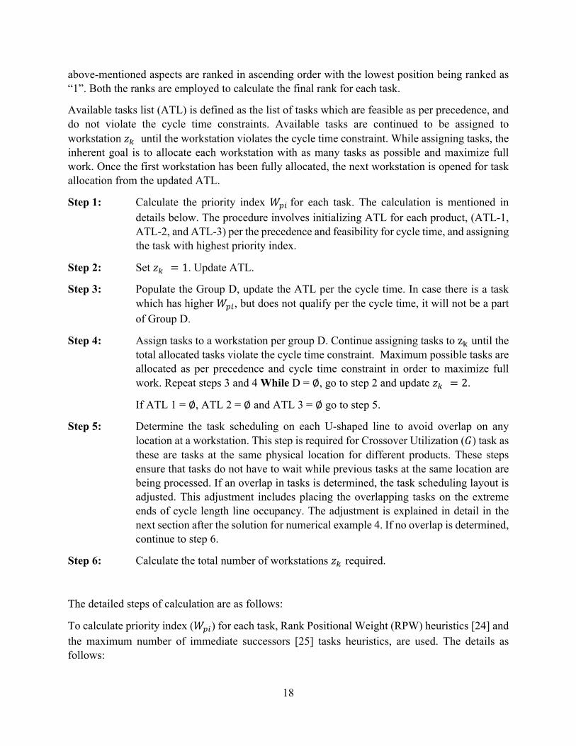
above-mentioned aspects are ranked in ascending order with the lowest position being ranked as “1”. Both the ranks are employed to calculate the final rank for each task.
Available tasks list (ATL) is defined as the list of tasks which are feasible as per precedence, and do not violate the cycle time constraints. Available tasks are continued to be assigned to workstation 𝑧[ until the workstation violates the cycle time constraint. While assigning tasks, the inherent goal is to allocate each workstation with as many tasks as possible and maximize full work. Once the first workstation has been fully allocated, the next workstation is opened for task allocation from the updated ATL.
Step 1: Calculate the priority index 𝑊~Lfor each task. The calculation is mentioned in details below. The procedure involves initializing ATL for each product, (ATL-1, ATL-2, and ATL-3) per the precedence and feasibility for cycle time, and assigning the task with highest priority index.
Step 2: Set 𝑧[ = 1. Update ATL.
Step 3: Populate the Group D, update the ATL per the cycle time. In case there is a task which has higher 𝑊~L, but does not qualify per the cycle time, it will not be a part of Group D.
Step 4: Assign tasks to a workstation per group D. Continue assigning tasks to z�until the total allocated tasks violate the cycle time constraint. Maximum possible tasks are allocated as per precedence and cycle time constraint in order to maximize full work. Repeat steps 3 and 4 While D = ∅, go to step 2 and update 𝑧[ = 2.
If ATL 1 = ∅, ATL 2 = ∅ and ATL 3 = ∅ go to step 5.
Step 5: Determine the task scheduling on each U-shaped line to avoid overlap on any location at a workstation. This step is required for Crossover Utilization (𝐺) task as these are tasks at the same physical location for different products. These steps ensure that tasks do not have to wait while previous tasks at the same location are being processed. If an overlap in tasks is determined, the task scheduling layout is adjusted. This adjustment includes placing the overlapping tasks on the extreme ends of cycle length line occupancy. The adjustment is explained in detail in the next section after the solution for numerical example 4. If no overlap is determined, continue to step 6.
Step 6: Calculate the total number of workstations 𝑧[required.
The detailed steps of calculation are as follows:
To calculate priority index (𝑊~L) for each task, Rank Positional Weight (RPW) heuristics [24] and the maximum number of immediate successors [25] tasks heuristics, are used. The details as follows:
19
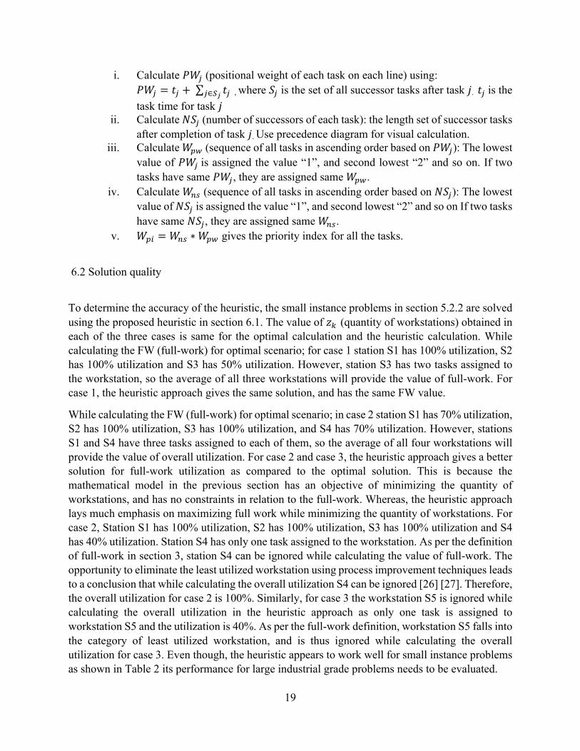
i. Calculate 𝑃𝑊K (positional weight of each task on each line) using: 𝑃𝑊K = 𝑡K + 𝑡KK∈�� , where 𝑆K is the set of all successor tasks after task 𝑗. 𝑡Kis the task time for task 𝑗
ii. Calculate 𝑁𝑆K (number of successors of each task): the length set of successor tasks after completion of task 𝑗. Use precedence diagram for visual calculation.
iii. Calculate 𝑊~� (sequence of all tasks in ascending order based on 𝑃𝑊K): The lowest value of 𝑃𝑊Kis assigned the value “1”, and second lowest “2” and so on. If two tasks have same 𝑃𝑊K, they are assigned same 𝑊~�.
iv. Calculate 𝑊V� (sequence of all tasks in ascending order based on 𝑁𝑆K): The lowest value of 𝑁𝑆Kis assigned the value “1”, and second lowest “2” and so on If two tasks have same 𝑁𝑆K, they are assigned same 𝑊V�.
v. 𝑊~L = 𝑊V� ∗ 𝑊~� gives the priority index for all the tasks.
6.2 Solution quality
To determine the accuracy of the heuristic, the small instance problems in section 5.2.2 are solved using the proposed heuristic in section 6.1. The value of 𝑧[(quantity of workstations) obtained in each of the three cases is same for the optimal calculation and the heuristic calculation. While calculating the FW (full-work) for optimal scenario; for case 1 station S1 has 100% utilization, S2 has 100% utilization and S3 has 50% utilization. However, station S3 has two tasks assigned to the workstation, so the average of all three workstations will provide the value of full-work. For case 1, the heuristic approach gives the same solution, and has the same FW value.
While calculating the FW (full-work) for optimal scenario; in case 2 station S1 has 70% utilization, S2 has 100% utilization, S3 has 100% utilization, and S4 has 70% utilization. However, stations S1 and S4 have three tasks assigned to each of them, so the average of all four workstations will provide the value of overall utilization. For case 2 and case 3, the heuristic approach gives a better solution for full-work utilization as compared to the optimal solution. This is because the mathematical model in the previous section has an objective of minimizing the quantity of workstations, and has no constraints in relation to the full-work. Whereas, the heuristic approach lays much emphasis on maximizing full work while minimizing the quantity of workstations. For case 2, Station S1 has 100% utilization, S2 has 100% utilization, S3 has 100% utilization and S4 has 40% utilization. Station S4 has only one task assigned to the workstation. As per the definition of full-work in section 3, station S4 can be ignored while calculating the value of full-work. The opportunity to eliminate the least utilized workstation using process improvement techniques leads to a conclusion that while calculating the overall utilization S4 can be ignored [26] [27]. Therefore, the overall utilization for case 2 is 100%. Similarly, for case 3 the workstation S5 is ignored while calculating the overall utilization in the heuristic approach as only one task is assigned to workstation S5 and the utilization is 40%. As per the full-work definition, workstation S5 falls into the category of least utilized workstation, and is thus ignored while calculating the overall utilization for case 3. Even though, the heuristic appears to work well for small instance problems as shown in Table 2 its performance for large industrial grade problems needs to be evaluated.

20
Table 2. Solution quality when comparing the optimal value and the heuristic value.
6.3 Numerical examples
The following four numerical examples are presented to illustrate the applicability of the proposed heuristic to industrial grade problems. The first three numerical examples have three products in consideration, and example 4 will tackle four products. This is done to ensure that the proposed heuristic is valid for more than three products. In example 4, all four products are balanced at the same time.
6.3.1 Input for numerical examples
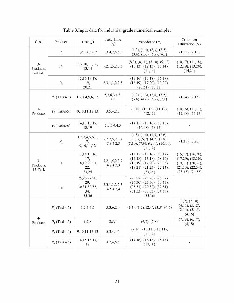
Cycle time for all the four numerical problems is ten (time-units). The input data is presented in Table 3
Case
Optimal Heuristic
time (CPU sec)
Solution (workstation number) 𝑧[ FW
Solution (workstation number) 𝑧[ FW
S1 S2 S3 S4 S5 S1 S2 S3 S4 S5
Case 1; 3-Products, 3-
Tasks 2
1,2,7 - -
3 0.833
1,2,7 - -
3 0.833 4 - - 4 - -
- 5,8 9,6 - 5,8 9,6
- 3 - - 3 -
Case 2; 3-Products, 4-
Tasks 8
9,1,2 - 10,3 -
4 0.85
1 2,3,9,4 - -
4 1 - 5 6 - 5,6 - - -
- 11,12 - 7,8 - - 7,11,8 12
- - - 4 - - 10 -
Case 3; 3-Products, 5-
Tasks 333
1,11,12 2,3,4 - - -
5 0.86
1,11,12 2 - - -
5 . 975 - - - - 6 - 6,7,8 13,14 - -
- - 7,13 14,8,9 15,10 - - 9,10 - 15
- - 5 - - - - - 3,4,5 -
21
Table 3.Input data for industrial grade numerical examples
Case Product Task (𝑗) Task Time
(𝑡K) Precedence (𝑷) Crossover
Utilization (𝐺)
3-Products, 7-Task
𝑃' 1,2,3,4,5,6,7 1,3,4,2,5,6,5 (1,2), (1,4), (2,3), (2,5), (3,6), (5,6), (6,7), (4,7) (1,15), (2,16)
𝑃( 8,9,10,11,12, 13,14 5,2,1,5,2,3,3
(8,9), (8,11), (8,10), (9,12), (10,13), (12,13), (13,14),
(11,14)
(10,17), (11,18), (12,19), (13,20),
(14,21)
𝑃* 15,16,17,18,
19, 20,21
2,3,1,3,2,2,5 (15,16), (15,18), (16,17), (16,19), (17,20), (19,20),
(20,21), (18,21) -
3-Products
𝑃'(Tasks-8) 1,2,3,4,5,6,7,8 5,3,6,3,4,3, 4,3
(1,2), (1,3), (2,4), (3,5), (5,6), (4,6), (6,7), (7,8) (1,14), (2,15)
𝑃((Tasks-5) 9,10,11,12,13 3,5,4,2,3 (9,10), (10,12), (11,12), (12,13)
(10,16), (11,17), (12,18), (13,19)
𝑃*(Tasks-6) 14,15,16,17, 18,19 5,3,3,4,4,5 (14,15), (15,16), (17,16),
(16,18), (18,19) -
3-Products, 12-Task
𝑃' 1,2,3,4,5,6,7,
8, 9,10,11,12
5,2,2,5,2,3,4,7,3,4,2,3
(1,3), (1,4), (1,5), (2,6), (3,6), (6,7), (4,7), (5,8),
(8,10), (7,9), (9,11), (10,11), (11,12)
(1,25), (2,26)
𝑃(
13,14,15,16, 17,
18,19,20,21, 22,
23,24
5,2,1,5,2,3,7,4,2,4,3,3
(13,15), (13,16), (13,17), (14,18), (15,18), (18,19), (16,19), (17,20), (20,22), (19,21), (21,23), (22,23),
(23,24)
(15,27), (16,28), (17,29), (18,30), (19,31), (20,32), (21,33), (22,34), (23,35), (24,36)
𝑃*
25,26,27,28, 29,
30,31,32,33, 34,
35,36
2,3,1,3,2,2,3,4,5,4,3,4
(25,27), (25,28), (25,29), (26,30), (27,30), (30,31), (28,31), (29,32), (32,34), (31,33), (33,35), (34,35),
(35,36)
-
4-Products
𝑃' (Tasks-5) 1,2,3,4,5 5,3,6,2,4 (1,3), (1,2), (2,4), (3,5), (4,5)
(1,9), (2,10), (4,11), (5,12), (2,14), (3,15),
(4,16)
𝑃( (Tasks-3) 6,7,8 3,5,4 (6,7), (7,8) (7,13), (6,17), (8,18)
𝑃* (Tasks-5) 9,10,11,12,13 5,3,4,4,5 (9,10), (10,11), (13,11), (11,12) -
𝑃� (Tasks-5) 14,15,16,17, 18 3,2,4,5,6 (14,16), (16,18), (15,18),
(17,18) -
22
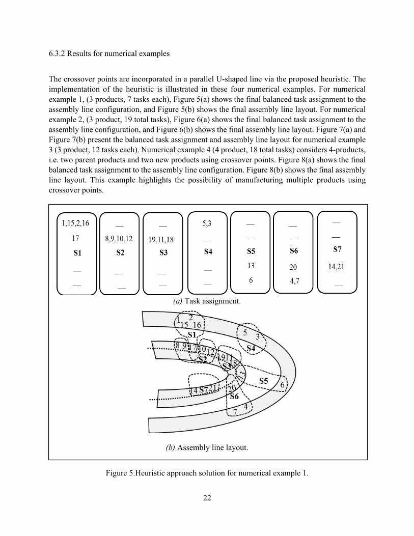
6.3.2 Results for numerical examples
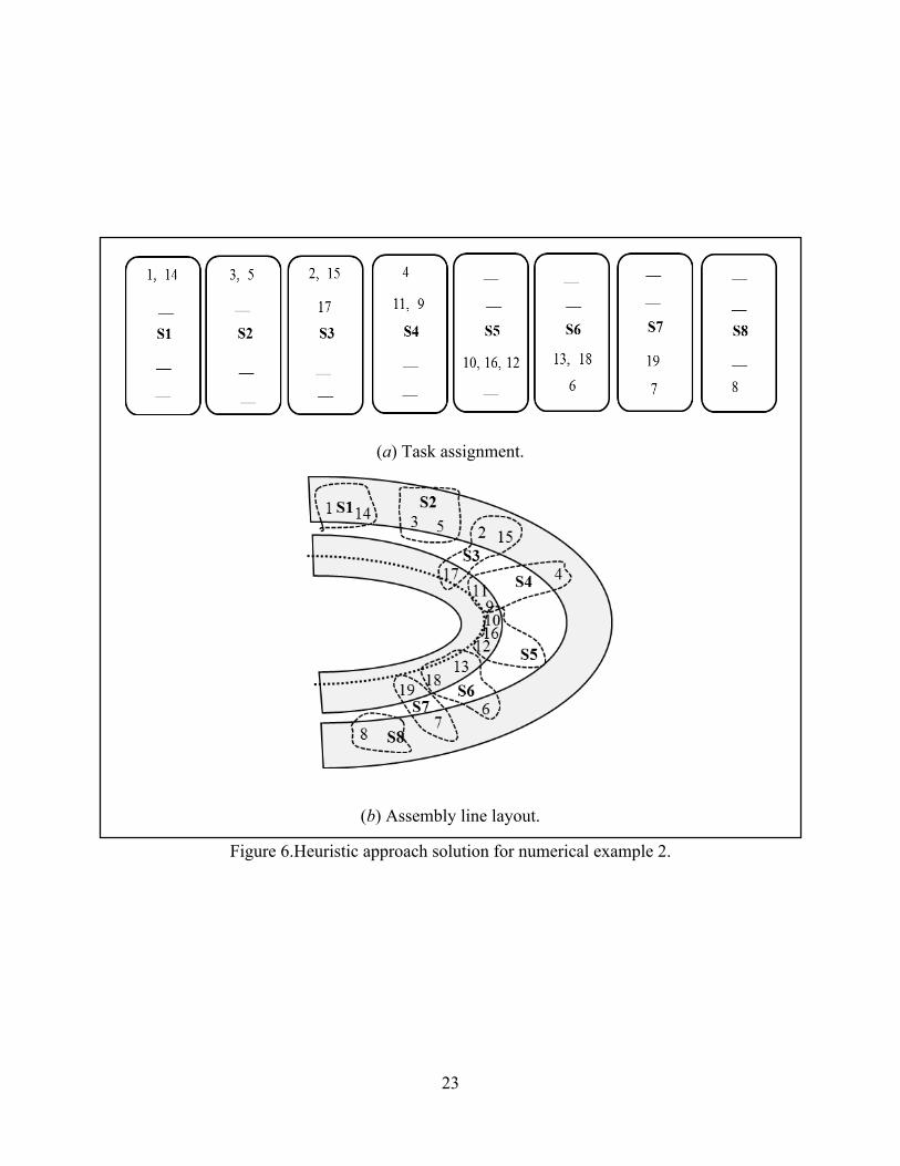
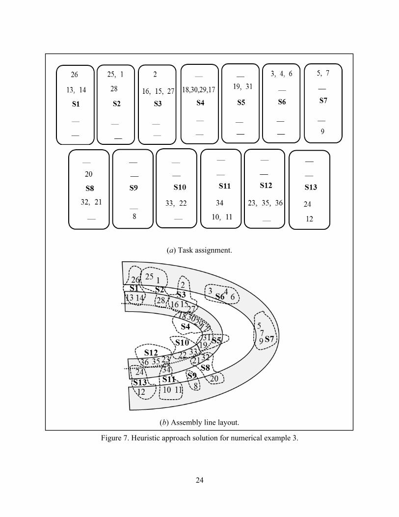
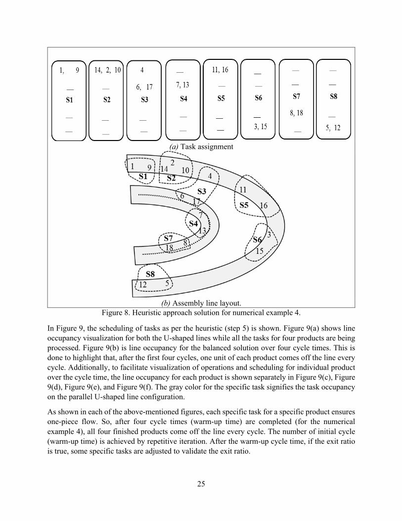
The crossover points are incorporated in a parallel U-shaped line via the proposed heuristic. The implementation of the heuristic is illustrated in these four numerical examples. For numerical example 1, (3 products, 7 tasks each), Figure 5(a) shows the final balanced task assignment to the assembly line configuration, and Figure 5(b) shows the final assembly line layout. For numerical example 2, (3 product, 19 total tasks), Figure 6(a) shows the final balanced task assignment to the assembly line configuration, and Figure 6(b) shows the final assembly line layout. Figure 7(a) and Figure 7(b) present the balanced task assignment and assembly line layout for numerical example 3 (3 product, 12 tasks each). Numerical example 4 (4 product, 18 total tasks) considers 4-products, i.e. two parent products and two new products using crossover points. Figure 8(a) shows the final balanced task assignment to the assembly line configuration. Figure 8(b) shows the final assembly line layout. This example highlights the possibility of manufacturing multiple products using crossover points.
(a) Task assignment.
(b) Assembly line layout.
Figure 5.Heuristic approach solution for numerical example 1.
23
(a) Task assignment.
(b) Assembly line layout.
Figure 6.Heuristic approach solution for numerical example 2.
24
(a) Task assignment.
(b) Assembly line layout.
Figure 7. Heuristic approach solution for numerical example 3.
25
(a) Task assignment
(b) Assembly line layout.
Figure 8. Heuristic approach solution for numerical example 4.
In Figure 9, the scheduling of tasks as per the heuristic (step 5) is shown. Figure 9(a) shows line occupancy visualization for both the U-shaped lines while all the tasks for four products are being processed. Figure 9(b) is line occupancy for the balanced solution over four cycle times. This is done to highlight that, after the first four cycles, one unit of each product comes off the line every cycle. Additionally, to facilitate visualization of operations and scheduling for individual product over the cycle time, the line occupancy for each product is shown separately in Figure 9(c), Figure 9(d), Figure 9(e), and Figure 9(f). The gray color for the specific task signifies the task occupancy on the parallel U-shaped line configuration.
As shown in each of the above-mentioned figures, each specific task for a specific product ensures one-piece flow. So, after four cycle times (warm-up time) are completed (for the numerical example 4), all four finished products come off the line every cycle. The number of initial cycle (warm-up time) is achieved by repetitive iteration. After the warm-up cycle time, if the exit ratio is true, some specific tasks are adjusted to validate the exit ratio.

26
(a) Line occupancy per cycle time for the balanced lines for numerical example 4.
(b) Line occupancy for each corresponding task
(c) Line occupancy for each corresponding task for product 𝑃'
(d) Line occupancy for each corresponding task for product 𝑃(
(e) Line occupancy for each corresponding task for product 𝑃*
(f) Line occupancy for each corresponding task for product 𝑃�
Figure 9. Line occupancy and scheduling display for numerical example 4
STATION7
STATION4
STATION3LINE2 0 10
STATION8
STATION6
STATION5
STATION3
STATION2
STATION10 10
LINE1
7 13
8 18
5 12
6 17
11 16
3 15
4
14 2 10
1 9
STATION8
STATION6
STATION5
STATION3
STATION2
STATION10 10 20 30 40
LINE1
14 2 10
1 9 1 9 1 9 1 9
14 2 10 14 2 10 14 2 10
3 15 3 15 3 15 3 15
11 16 11 16 11 16 11 16
5 12 5 12 5 12 5 12
4 4 4 4
STATION7
STATION4
STATION3LINE2 0 10 20 30 40
6 17 6 17
8 18 8 18
7 13 7 13 7 13 7 13
6 17 6 17
8 18 8 18
STATION7
STATION4
STATION3LINE2 0 10 20 30 40
STATION8
STATION6
STATION5
STATION3
STATION2
STATION10 10 20 30 40
LINE1
13
2 10 14 2 10 14 2 10
1 9 1 9 1 9 1 9
11 16 11 16 11 16 11 16
4 4 4 4
5 12 5 12
3 15 3 15 3 15 3 15
7 13 7 13
6 17 6 17 6 17 6 17
8 18 8 18 8 18 8 18
14 2 10 14
5 12 5 12
7 7 13
STATION7
STATION4
STATION3LINE2 0 10 20 30 40
STATION8
STATION6
STATION5
STATION3
STATION2
STATION10 10 20 30 40
LINE1
2 10
1 9 1 9 1 9 1 9
4 4 4 4
14 2 10 14 2 10 14 2 10 14
3 15 3 15
11 16 11 16 11 16 11 16
6 17 6 17
5 12 5 12 5 12 5 12
8 18 8 18
7 7 13 7 13 7 1313
3 15 3 15
6 17 6 17
8 18 8 18
STATION7
STATION4
STATION3LINE2 0 10 20 30 40
STATION8
STATION6
STATION5
STATION3
STATION2
STATION10 10 20 30 40
LINE1
1 91 9 1 9 1 9
14 2 10 14 2 10
4 4 4 4
14 2 10 14 2 10
3 15
11 16 11 16 11 16 11 16
3 15 3 15 3 15
6 17
5 12 5 12 5 12 5 12
6 17 6 17 6 17
8 18
7 13 7 13 7 13 7 13
8 18 8 18 8 18
1 2 3 4 Cycle
27
For example: for 𝑃(, task 6 is performed in warm-up cycle 2, task 7 is performed in warm-up cycle 3, and task 8 is performed in warm-up cycle 4. This is done to ensure that the exit ratio and one-piece flow holds true. For this case, finished𝑃', 𝑃*, and 𝑃� exits the after 4 warm-up cycles. After the initial adjustment is made for 𝑃(; one of each product comes off the line every cycle.
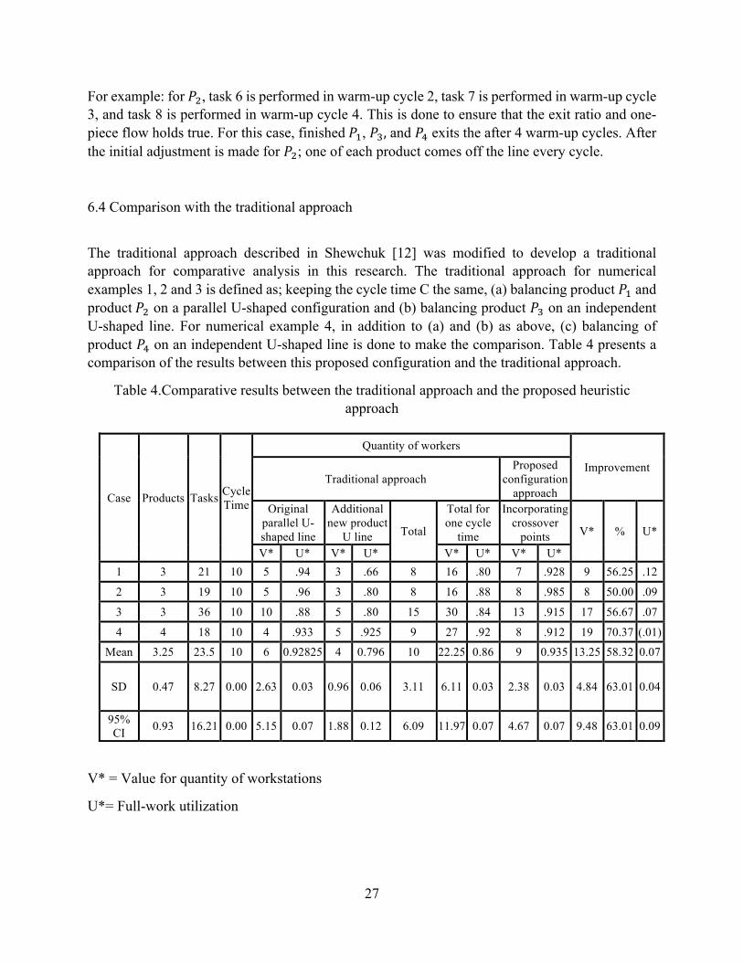
6.4 Comparison with the traditional approach
The traditional approach described in Shewchuk [12] was modified to develop a traditional approach for comparative analysis in this research. The traditional approach for numerical examples 1, 2 and 3 is defined as; keeping the cycle time C the same, (a) balancing product 𝑃' and product𝑃( on a parallel U-shaped configuration and (b) balancing product 𝑃* on an independent U-shaped line. For numerical example 4, in addition to (a) and (b) as above, (c) balancing of product 𝑃� on an independent U-shaped line is done to make the comparison. Table 4 presents a comparison of the results between this proposed configuration and the traditional approach.
Table 4.Comparative results between the traditional approach and the proposed heuristic approach
V* = Value for quantity of workstations
U*= Full-work utilization
Case Products Tasks Cycle Time
Quantity of workers
Improvement Traditional approach
Proposed configuration
approach Original
parallel U-shaped line
Additional new product
U line Total
Total for one cycle
time
Incorporating crossover
points V* % U*
V* U* V* U* V* U* V* U* 1 3 21 10 5 .94 3 .66 8 16 .80 7 .928 9 56.25 .12
2 3 19 10 5 .96 3 .80 8 16 .88 8 .985 8 50.00 .09
3 3 36 10 10 .88 5 .80 15 30 .84 13 .915 17 56.67 .07
4 4 18 10 4 .933 5 .925 9 27 .92 8 .912 19 70.37 (.01)
Mean 3.25 23.5 10 6 0.92825 4 0.796 10 22.25 0.86 9 0.935 13.25 58.32 0.07
SD 0.47 8.27 0.00 2.63 0.03 0.96 0.06 3.11 6.11 0.03 2.38 0.03 4.84 63.01 0.04
95% CI 0.93 16.21 0.00 5.15 0.07 1.88 0.12 6.09 11.97 0.07 4.67 0.07 9.48 63.01 0.09

28
The effectiveness of this proposed heuristic for larger sized industrial problems is demonstrated in the four numerical example problems. As described in section 5.4, all the four numerical problems are large sized and solving them mathematically is intractable. Since the optimal value cannot be obtained in the cases where associated number of tasks is high, the proposed heuristic value gives a feasible solution. Section 6.2 demonstrates that the value for the number of workstations required via heuristic approach is equal to the value obtained via optimal approach.
There is an established benchmark approach which is referred as current best approach, and any proposed heuristic is compared to it. Since the proposed approach is a new problem, there is currently no best heuristic approach available for comparison. Also, this proposed configuration is an initial research which introduces crossover points. Non-availability of any research literature in this kind of proposed configuration, results in non-availability of any current best heuristic. Therefore, to obtain a comparative analysis, a traditional approach is used.
In the traditional approach for case 1 (3 products, 7 tasks each), 𝑃' and 𝑃( are assembled on original parallel U-shaped line, and exit the line in one cycle time (ten time-units). 𝑃* is manufactured on additional U-shaped line, and exits the line in one cycle time (ten time-units). At the end of two cycle time (twenty time-units), finished products which exit the line are 1 𝑃', 1 𝑃(, and 1 𝑃*. In order to compare the number of workstations required in one cycle time, for the traditional approach the value of total in case 1 is multiplied by 2. This multiplication is valid for cases 1, 2, and 3. For case 4, the multiplication factor is 3. This multiplication factor accounts for the requirement of time to produce the same number of finished products. Also, this comparison showcases higher resource utilization in the case of using crossover points in a parallel U-shaped line configuration.
In Table 4, U* and V* are the full-work, and the total quantity of workstations required respectively, for all four numerical examples. Full-work calculation utilized the formulae mentioned in section 3. The value of U* highlights the benefit of crossover points as for an already high value of utilization in a parallel U-shaped line, a reduction of approximately 60% in number workstation is achieved. Only for case 4, there is a 1% reduction in full-work. The other three cases show improvement in full-work, and a reduction in the number of workstation required. Case 4 signifies that if the workstation utilization is already high, using this proposed configuration may lead to reduction in the number of workstations, but improving full-work value may not be possible.
In the heuristic approach for case 1, three products𝑃',𝑃(, and 𝑃* are assembled at the same time and all three finished products exit the line at the end of one cycle time (ten time-units). Table 4 shows that the proposed approach of incorporating crossover points has performed better when compared to a traditional approach.
29
7. DISCUSSION
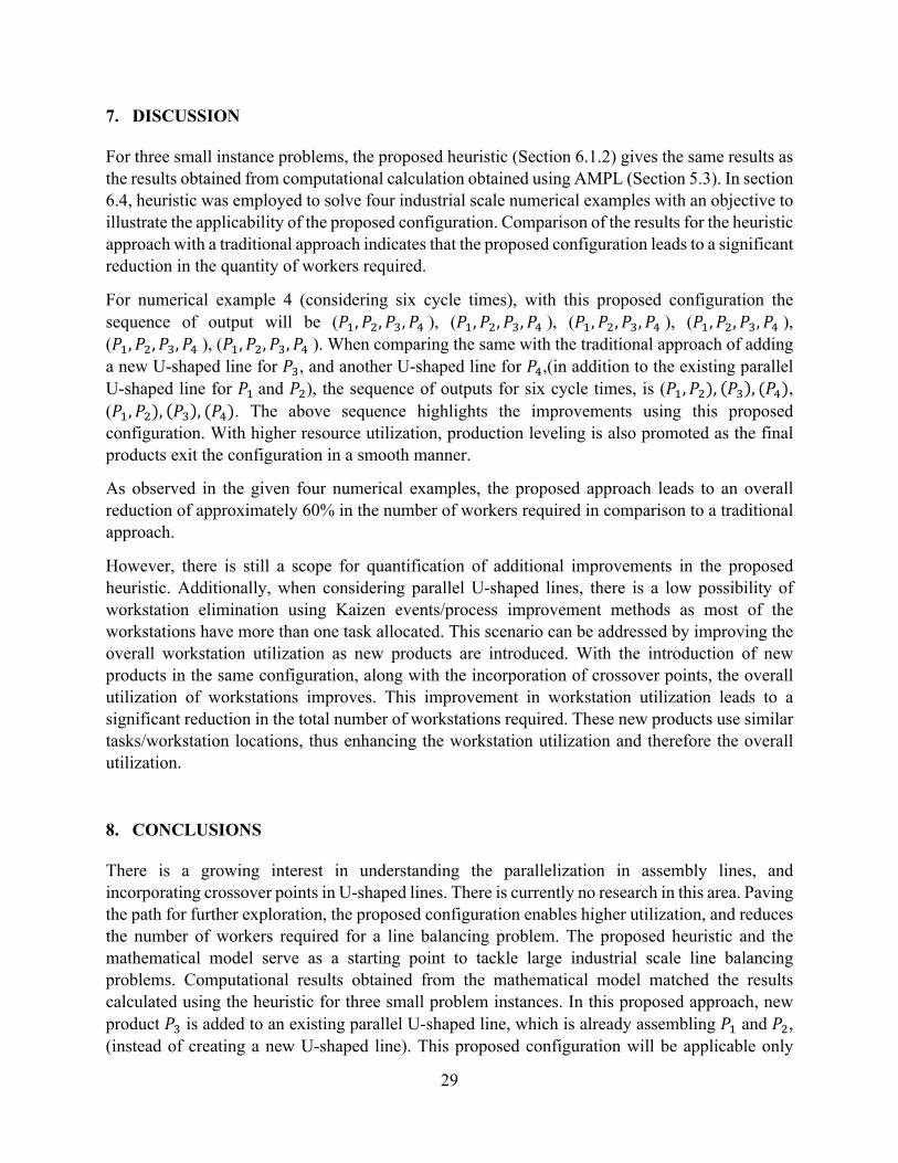
For three small instance problems, the proposed heuristic (Section 6.1.2) gives the same results as the results obtained from computational calculation obtained using AMPL (Section 5.3). In section 6.4, heuristic was employed to solve four industrial scale numerical examples with an objective to illustrate the applicability of the proposed configuration. Comparison of the results for the heuristic approach with a traditional approach indicates that the proposed configuration leads to a significant reduction in the quantity of workers required.
For numerical example 4 (considering six cycle times), with this proposed configuration the sequence of output will be (𝑃', 𝑃(, 𝑃*, 𝑃�), (𝑃', 𝑃(, 𝑃*, 𝑃�), (𝑃', 𝑃(, 𝑃*, 𝑃�), (𝑃', 𝑃(, 𝑃*, 𝑃�), (𝑃', 𝑃(, 𝑃*, 𝑃�), (𝑃', 𝑃(, 𝑃*, 𝑃�). When comparing the same with the traditional approach of adding a new U-shaped line for 𝑃*, and another U-shaped line for 𝑃�,(in addition to the existing parallel U-shaped line for 𝑃'and 𝑃(), the sequence of outputs for six cycle times, is (𝑃', 𝑃(), 𝑃* , (𝑃�), (𝑃', 𝑃(), 𝑃* , (𝑃�). The above sequence highlights the improvements using this proposed configuration. With higher resource utilization, production leveling is also promoted as the final products exit the configuration in a smooth manner.
As observed in the given four numerical examples, the proposed approach leads to an overall reduction of approximately 60% in the number of workers required in comparison to a traditional approach.
However, there is still a scope for quantification of additional improvements in the proposed heuristic. Additionally, when considering parallel U-shaped lines, there is a low possibility of workstation elimination using Kaizen events/process improvement methods as most of the workstations have more than one task allocated. This scenario can be addressed by improving the overall workstation utilization as new products are introduced. With the introduction of new products in the same configuration, along with the incorporation of crossover points, the overall utilization of workstations improves. This improvement in workstation utilization leads to a significant reduction in the total number of workstations required. These new products use similar tasks/workstation locations, thus enhancing the workstation utilization and therefore the overall utilization.
8. CONCLUSIONS There is a growing interest in understanding the parallelization in assembly lines, and incorporating crossover points in U-shaped lines. There is currently no research in this area. Paving the path for further exploration, the proposed configuration enables higher utilization, and reduces the number of workers required for a line balancing problem. The proposed heuristic and the mathematical model serve as a starting point to tackle large industrial scale line balancing problems. Computational results obtained from the mathematical model matched the results calculated using the heuristic for three small problem instances. In this proposed approach, new product 𝑃* is added to an existing parallel U-shaped line, which is already assembling 𝑃' and 𝑃(, (instead of creating a new U-shaped line). This proposed configuration will be applicable only
30
when there is sufficient spare capacity available on the original parallel U-shaped line. So, if the product family being assembled on the proposed configuration has characteristics which are inherent to products assembled on U-shaped lines, the implementation of crossover points will bring immense success. Some of the characteristics involved are that all the products are mid-volume, and the setup/changeover time for machine locations (when switching between tasks for different products) is negligible.
The proposed heuristic uses two well-known line balancing heuristics to calculate priority index for each task. Four different industrial grade numerical examples are solved using the proposed heuristic to establish the advantages of the crossover points. The results obtained from the proposed configuration show approximately 60% reduction in the number of workstations required in comparison to a traditional approach of independent assembly lines for different products. Thus, the benefits of the parallel U-shaped lines with crossover points are explored and illustrated in this research. This proposed configuration has many promising practical applications in the industrial sector. While establishing new products via crossover points, savings are established as the number of workstations required is reduced.
As the initial research in the field of parallel U-shaped assembly lines with crossover points, this study can yield many research extensions. Some research extensions are:
(a) Determination of the conditions (data sets) under which heuristic will provide optimal solution. Once these conditions are determined, the heuristic can be called an exact algorithm.
(b) Problem structure is modified in such a way that the greedy approach in heuristic results in optimal solution.
(c) The mathematical model can be further refined to take the walking time of workers into consideration.
(d) Helper tasks can be included in this proposed configuration to attain higher station utilization.
31
REFERENCES
[1] J. Miltenburg, "Balancing U-lines in a multiple U-line facility," European Journal of Operational Research, pp. 1-23, 1998.
[2] T. L. Urban, "Optimal balancing of U-shaped assembly lines," Management Science, pp. 738-741, 1998.
[3] J. Miltenburg and D. Sparling , "Optimal solution algorithms for the U-line balancing problem," Relatrio tecnico, McMaster University, Hamilton, Canada. Citado na, 1995.
[4] M. E. Salveson, "The assembly line balancing problem," Journal of industrial engineering, pp. 18-25, 1955.
[5] Y. K. Kim, S. J. Kim and J. Y. Kim, "Balancing and sequencing mixed-model U-lines with a co-evolutionary algorithm," Production Planning & Control, pp. 754-764, 2000.
[6] M. Sali and E. Sahin, "Line feeding optimization for Just in Time assembly lines: An application to the automotive industry," International Journal of Production Economics, pp. 54-67, 2016.
[7] T. Ohno, Toyota production system: beyond large-scale production, crc Press, 1988.
[8] H. Gokccen, K. Augpak and R. Benzer, "Balancing of parallel assembly lines," International Journal of Production Economics, pp. 600-609, 2006.
[9] G. Miltenburg and J. Wijngaard, "The U-line line balancing problem," Management science, pp. 1378-1388, 1994.
[10] T. Korkmazel and S. Meral, "Bicriteria sequencing methods for the mixed-model assembly line in just-in-time production systems," European Journal of Operational Research, pp. 188-207, 2001.
[11] J. Miltenburg, "U-shaped production lines: A review of theory and practice," International Journal of Production Economics, pp. 201-214, 2001.
[12] J. P. Shewchuk, "Worker allocation in lean U-shaped production lines," International Journal of Production Research, pp. 3485-3502, 2008.
[13] gama.com, "Mercedes-Benz bus assembly plant," [Online]. Available: http://www.gama.com.tr/doc/image/projects/85/big/PfRkehaO.jpg.
[14] king-long, " Long bus assembly plant in China," [Online]. Available: http://f.etwservice.com/newsupfile/2010126135858901.jpg.
32
[15] yutong, "bus assembly line," [Online]. Available: http://www.yutong.com/english/images/news/press/2014/02/21/1249B1F58CA6D33B14C1A2DB12C9D089.jpg.
[16] U. Ozcan, H. Gokccen and B. Toklu, "Balancing parallel two-sided assembly lines," International Journal of Production Research, pp. 4767-4784, 2010.
[17] I. Kucukkoc and D. Z. Zhang, "Integrating ant colony and genetic algorithms in the balancing and scheduling of complex assembly lines," The International Journal of Advanced Manufacturing Technology, pp. 265-285, 2016.
[18] I. Kucukkoc and D. Z. Zhang, "Simultaneous balancing and sequencing of mixed-model parallel two-sided assembly lines," International Journal of Production Research, pp. 3665-3687, 2014.
[19] W.-C. Chiang, P. Kouvelis and T. L. Urban, "Line balancing in a just-in-time production environment: balancing multiple U-lines," IIE Transactions, pp. 347-359, 2007.
[20] J. P. Shewchuk, "U-line Design and Operation with Helper Tasks," in U-line Design and Operation with Helper Tasks, 2012.
[21] I. Kucukkoc and D. Z. Zhang , "Balancing of parallel U-shaped assembly lines," Computers & Operations Research, pp. 233-244, 2015.
[22] "ampl," [Online]. Available: http://ampl.com/. [Accessed 11 05 2017].
[23] "ampl," [Online]. Available: http://ampl.com/products/solvers/solvers-we-sell/knitro/. [Accessed 11 06 2017].
[24] W. Helgeson and D. Birnie, "Assembly line balancing using the ranked positional weight technique," Journal of Industrial Engineering, pp. 394-398, 1961.
[25] F. M. Tonge, "Summary of a heuristic line balancing procedure," Management Science, no. INFORMS, pp. 21-42, 1960.
[26] P. Dennis, Lean Production simplified: A plain-language guide to the world's most powerful production system, Crc press, 2016.
[27] K. Suzaki, New manufacturing challenge: Techniques for continuous improvement, Simon and Schuster, 1987.
33
APPENDIX A AMPL code for parallel U-shaped assembly lines with crossover points. ##parameters##
param n; # number of tasks
param n1; # number of tasks on Line1 outside U-line
param n2; # number of tasks on Line2 inside U-line
param e; # number of edges
param c; #cycle time
param m; # kmax for me
param g; #tasks in the crossover product
param t{j in 1..n}; # task times of J tasks
param N1 {j in 1..n1}; #task number of task on Line L1
param N2 {j in 1..n2}; #task number of task on Line L2
##sets##
param P {j in 1..e, k in 1..2}; #precedence
param N {j in 1..g, k in 1..2}; #replicated tasks
##variables##
var v {j in 1..n, k in 1..m} binary;#front of the outer line
var x {j in 1..n, k in 1..m} binary;#front of the inner line
var y {j in 1..n, k in 1..m} binary;#back of the inner line
var w {j in 1..n, k in 1..m} binary;#back of the outer line
var z {k in 1..m} binary;
##objective function##
minimize workers: (sum{k in 1..m} z[k]);
##contrainsts##
subject to limit {j in 1..n}: sum {k in 1..m} (v[j, k] + x[j, k] + y[j, k] + w[j, k]) = 1;
# assignment constraint1.

34
subject to cycle_time {k in 1..m} : sum {j in 1..n} ((v[j, k] + x[j, k] + y[j, k] + w[j, k]) * t[j]) <= c*(z[k]);
# cycle time Capacity constraint.
subject to FWDPREV {j in 1..e}: sum{k in 1..m} ((m - k + 1) * (v[P[j,1], k] - v[P[j,2], k])) >= 0 ;
# Forward precedence for variable v
subject to FWDPREX {j in 1..e}: sum{k in 1..m} ((m - k + 1) * (x[P[j,1], k] - x[P[j,2], k])) >= 0 ;
# Forward precedence for variable x
subject to BWDPREY {j in 1..e}: sum {k in 1..m} ((m - k + 1) * (y[P[j,2], k] - y[P[j,1], k])) >= 0 ;
# Backward precedence for variable y
subject to BWDPREW {j in 1..e}: sum {k in 1..m} ((m - k + 1) * (w[P[j,2], k] - w[P[j,1], k])) >= 0 ;
# Backward precedence for variable w
subject to positionalcon1 {k in 1..m,j in 1..n,i in 1..n}:(x[i, k] + w[j, k]) <= 1;
# Positional constraint 1.
subject to positionalcon2 {k in 1..m,j in 1..n,i in 1..n}:(w[i, k] + v[j, k] ) <= 1;
# Positional constraint 2.
subject to positionalcon3 {k in 1..m,j in 1..n,i in 1..n}:(y[i, k] + v[j, k] ) <= 1;
# Positional constraint 3
subject to producttaskplacement1 {k in 1..m} : (sum {j in 1..n1} (x[N1[j], k] + y[N1[j], k])) <= 0;
# Product task placement 1
subject to producttaskplacement3 {k in 1..m} : (sum {j in 1..n2} (v[N2[j], k] + w[N2[j], k])) <= 0;
# Product task placement 3
subject to crossovercon1 {i in 1..g} :
(sum {k in 1..m} (x[N[i,1], k] - x[N[i,2], k])) <= 0;
subject to crossovercon2 {i in 1..g} :
(sum {k in 1..m} (x[N[i,2], k] - x[N[i,1], k])) <= 0;
35
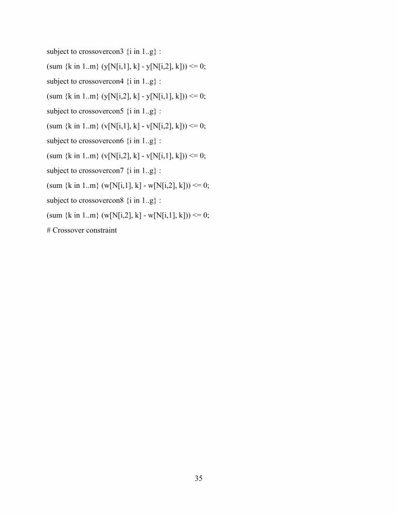
subject to crossovercon3 {i in 1..g} :
(sum {k in 1..m} (y[N[i,1], k] - y[N[i,2], k])) <= 0;
subject to crossovercon4 {i in 1..g} :
(sum {k in 1..m} (y[N[i,2], k] - y[N[i,1], k])) <= 0;
subject to crossovercon5 {i in 1..g} :
(sum {k in 1..m} (v[N[i,1], k] - v[N[i,2], k])) <= 0;
subject to crossovercon6 {i in 1..g} :
(sum {k in 1..m} (v[N[i,2], k] - v[N[i,1], k])) <= 0;
subject to crossovercon7 {i in 1..g} :
(sum {k in 1..m} (w[N[i,1], k] - w[N[i,2], k])) <= 0;
subject to crossovercon8 {i in 1..g} :
(sum {k in 1..m} (w[N[i,2], k] - w[N[i,1], k])) <= 0;
# Crossover constraint