NC STATE UNIVERSITY

Balancing biomass harvesting and drying tactics with delivered payment practice

Refining woody biomass feedstock logistics

Dr. Joseph P Roise, Dr. Glenn Catts, Dr. Dennis Hazel, Dr. Alex Hobbs, and Chris Hopkins

12/23/2013

North Carolina State University wishes to acknowledge financial support by the USDA Forest

Service and the U.S. Endowment for Forestry and Communities that made this work possible.

ABSTRACT: This is a report on a study which values woody biomass (per ton) as a function of moisture content (MC), time and logistics. Wood’s net energy content is inversely related to MC. Purchasers of woody biomass are keenly aware of MC, since net energy can vary by up to 240% from green to bone dry wood. Wood dries at a predictable rate, which is a function of weather variables. A tractor trailer load of green wood is limited by gross weight restrictions for a highway truck, however the same trailer with less than 22% MC is limited by the trailer’s volume. A trailer loaded with drier wood can haul significantly more energy. A field drying and logistics methodology that reduces the moisture content of woody biomass is analyzed and the net value of a ton of biomass FOB as a function of MC is estimated.

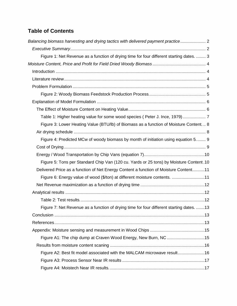
Table of Contents

Balancing biomass harvesting and drying tactics with delivered payment practice ..................... 2

Executive Summary ................................................................................................................ 2

Figure 1: Net Revenue as a function of drying time for four different starting dates. ........ 3

Moisture Content, Price and Profit for Field Dried Woody Biomass ............................................ 4

Introduction ............................................................................................................................ 4

Literature review ..................................................................................................................... 4

Problem Formulation .............................................................................................................. 5

Figure 2: Woody Biomass Feedstock Production Process. .............................................. 5

Explanation of Model Formulation .......................................................................................... 6

The Effect of Moisture Content on Heating Value ................................................................ 6

Table 1: Higher heating value for some wood species ( Peter J. Ince, 1979) ................... 7

Figure 3: Lower Heating Value (BTU/lb) of Biomass as a function of Moisture Content. .. 8

Air drying schedule ............................................................................................................. 8

Figure 4: Predicted MCw of woody biomass by month of initiation using equation 5. ....... 9

Cost of Drying ..................................................................................................................... 9

Energy / Wood Transportation by Chip Vans (equation 7) ..................................................10

Figure 5: Tons per Standard Chip Van (120 cu. Yards or 25 tons) by Moisture Content .10

Delivered Price as a function of Net Energy Content a function of Moisture Content ..........11

Figure 6: Energy value of wood ($/ton) at different moisture contents. ...........................11

Net Revenue maximization as a function of drying time .....................................................12

Analytical results ...................................................................................................................12

Table 2: Test results. ......................................................................................................12

Figure 7: Net Revenue as a function of drying time for four different starting dates. .......13

Conclusion ............................................................................................................................13

References ............................................................................................................................13

Appendix: Moisture sensing and measurement in Wood Chips .............................................15

Figure A1: The chip dump at Craven Wood Energy, New Burn, NC ...............................15

Results from moisture content scaning ..............................................................................16

Figure A2: Best fit model associated with the MALCAM microwave result ......................16

Figure A3: Process Sensor Near IR results ....................................................................17

Figure A4: Moistech Near IR results. ..............................................................................17

Balancing biomass harvesting and drying tactics with

delivered payment practice

Executive Summary

In this report we substantiate the assumption that dry biomass is worth much more per ton to the

purchaser than the delivery of wet biomass and that letting wood dry for up to a year is a profitable

investment for the biomass producer as long as the purchaser pays for wood, or energy, delivery

and not water delivery.

Nobody in the biomass energy industry wants to pay for water. Water does not burn. It costs money and energy to get rid of, and all biomass is about ½ water at time of harvest.

The methodology we developed reduces the moisture content of woody biomass, which increases the net energy content per ton, decreases the harvest and transportation cost per ton and increases the net value of a ton of biomass.

In cooperation with the North Carolina Association of Professional Loggers we developed

efficient methods for harvesting whole trees, removing moisture from the biomass and delivering

dry wood to the purchaser. Hardwood or softwood loggers need to handle large volumes

quickly. They need something substantial to grab and put into the chipper, a pulpwood stick.

This yields significantly more volume per hour of chipping, than when using tops and limbs

alone.

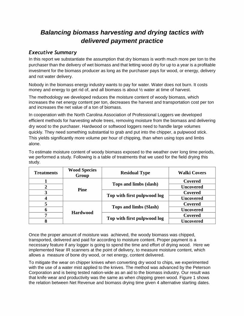
To estimate moisture content of woody biomass exposed to the weather over long time periods, we performed a study. Following is a table of treatments that we used for the field drying this study.

Treatments Wood Species

Group Residual Type Walki Covers

1

Pine

Tops and limbs (slash) Covered

2 Uncovered

3 Top with first pulpwood log

Covered

4 Uncovered

5

Hardwood

Tops and limbs (Slash) Covered

6 Uncovered

7 Top with first pulpwood log

Covered

8 Uncovered

Once the proper amount of moisture was achieved, the woody biomass was chipped, transported, delivered and paid for according to moisture content. Proper payment is a necessary feature if any logger is going to spend the time and effort of drying wood. Here we implemented Near IR scanners at the point of delivery, to measure moisture content, which allows a measure of bone dry wood, or net energy, content delivered.

To mitigate the wear on chipper knives when converting dry wood to chips, we experimented with the use of a water mist applied to the knives. The method was advanced by the Peterson Corporation and is being tested nation-wide as an aid to the biomass industry. Our result was that knife wear and productivity was the same as when chipping green wood. Figure 1 shows the relation between Net Revenue and biomass drying time given 4 alternative starting dates.

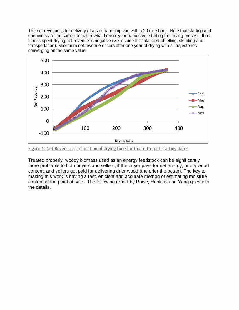
The net revenue is for delivery of a standard chip van with a 20 mile haul. Note that starting and endpoints are the same no matter what time of year harvested, starting the drying process. If no time is spent drying net revenue is negative (we include the total cost of felling, skidding and transportation). Maximum net revenue occurs after one year of drying with all trajectories converging on the same value.

Figure 1: Net Revenue as a function of drying time for four different starting dates.

Treated properly, woody biomass used as an energy feedstock can be significantly more profitable to both buyers and sellers, if the buyer pays for net energy, or dry wood content, and sellers get paid for delivering drier wood (the drier the better). The key to making this work is having a fast, efficient and accurate method of estimating moisture content at the point of sale. The following report by Roise, Hopkins and Yang goes into the details.

-100

0

100

200

300

400

500

0 100 200 300 400

Ne

t R

eve

nu

e

Drying date

Feb

May

Aug

Nov

Moisture Content, Price and Profit for Field Dried Woody

Biomass Joseph Roise, Chris Hopkins and Longjian Yang Professor, Research Assistant and Graduate Student, North Carolina State University

Introduction

All biomass energy producers from electric power generation to pellet manufacturers do not want to pay for water. Yet the predominant measure of value is delivered weight (tons in the Southeastern US). The purchaser assumes a market basket of wood with variable moisture content and pays an amount per delivered ton. This practice rewards suppliers who deliver wood as soon as it is cut and penalizes suppliers who deliver dry wood. (i.e. rewards people who deliver more water and penalizes people who deliver less water). Our study is based on what we now know about field biomass drying and harvesting, transport and delivery of woody biomass. The assumption is made that the purchaser of biomass will pay based on a measure of net energy (net energy is a function of moisture content) of the biomass, because purchasing biomass by weight does not reward the feed stock producer for delivering dry biomass. In order for the market to pay for net energy content at the point of trade a fast and efficient method to estimate moisture content is needed.

Literature review

Biomass is an important source of energy in the world and in the US biomass accounted for 53% of all renewable energy consumption in 2007. Wood energy, which includes wood fuel, wood byproducts, and wood waste comprises roughly 67% of total biomass energy consumption (Payne, 2012). A major problem associated with using wood as an energy source is that forest resources are distributed across the landscape and to supply feedstock to a wood using plant multiple operations including growing, harvesting, storage, pre-processing, transport, unloading and measuring the value of the delivered biomass need to occur. In agriculture, supply logistics are characterized by a randomly distributed raw material; time and weather-sensitive crop maturity; variable moisture content and a short time window for collection with competition from concurrent harvest operations (Ravula and others, 2007). Forest product supply logistics are similar, except for the short time window for harvesting.

Many people have studied and modeled the logistics associated with agriculture and forest products. Frombo and others (2009) buily a strategic decision model for planning woody biomass logistics for energy production. The optimization module is divided into three sub-modules to face different kinds of decision problems: strategic planning, tactical planning, and operational management. A combination multi-objective evolutionary algorithms (EMOO) and Mixed Integer Linear Programming (MILP) model was used by Fazlollahi and others (2011) to simultaneously minimize biomass feedstock costs and CO2 emission. Their results show that the simultaneous production of electricity and heat with biomass and natural gas are reliable when using the given assumptions. Mobini M. and others (2011) built a logistics model to evaluate the logistics of a biomass supply chain from forest harvesting areas to a potential power plant. This model is a simulation model based on the Integrated Biomass Supply Analysis and Logistics. This model includes three harvesting systems and the current method used in the study area is a conventional harvesting system for their area. “The simulation model is capable of providing estimates of cost, log volume, fuel volume, carbon emissions, and equilibrium moisture content of delivered material over the life span of the power plant”. Navarrete (2012) “developed and solved two optimal harvesting models for pine stands under price and wood stock stochastic diffusion, with risky decision agents, for single and multiple harvest rotation”.

He also tested the veracity of these two models and compared the effect of volatilities in the optimal business cutting policies. He found the multiple rotation model has increased rate of optimal deterministic solutions than the single rotation model, and “the impact of wood stock volatility in the optimal cut grows faster than price volatility”.

What is missing in these investigations is the effect of moisture content on the value of delivered biomass.

Problem Formulation

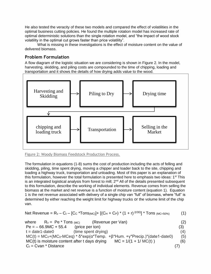
A flow diagram of the logistic situation we are considering is shown in Figure 2. In the model, harvesting, skidding, and piling costs are compounded to the time of chipping, loading and transportation and it shows the details of how drying adds value to the wood.

Figure 2: Woody Biomass Feedstock Production Process.

The formulation in equations (1-8) sums the cost of production including the acts of felling and skidding, piling, time spent drying, moving a chipper and loader back to the site, chipping and loading a highway truck, transportation and unloading. Most of this paper is an explanation of this formulation, however the total formulation is presented here to emphasis two ideas: 1st This is an integrated logistical analysis from forest to mill; 2nd All of the details presented subsequent to this formulation, describe the working of individual elements. Revenue comes from selling the biomass at the market and net revenue is a function of moisture content (equation 1). Equation 1 is the net revenue associated with delivery of a single chip van “full” of biomass, where “full” is

determined by either reaching the weight limit for highway trucks or the volume limit of the chip

van. Net Revenue = Rv – Ct – [CC *Tons(MC)]+ [(CH + CP) * (1 + r) (t/30)] * Tons (MC=50%) (1)

where Rv = Pe * Tons (MC) (Revenue per Van) (2) Pe = – 66.9MC + 55.4 (price per ton) (3) t = date1-date0 (time spent drying) (4) MC(t) = MC0+(MC0-MCeq) * δ*exp(α*Temp. +β*Hum. +γ*Precip.)*(date1-date0) (5) MC(t) is moisture content after t days drying MC = 1/(1 + 1/ MC(t) ) (6) Ct = Cvan * Distance (7)

Harvesting and Skidding

Piling to Dry Drying time

chipping and loading truck

TransportationSelling in the

Market

MC ≥ 0 Cvan: Cost per chip van per mile Ct: Cost of transportation CP: Cost of piling CH: Cost of harvesting and skidding biomass

CC: Cost of chipping and loading a highway truck + cost of returning to site.

Tons(MC) = {27.3 × MC + 18.9, MC < 23% 25, MC ≥ 23%

(8)

r = monthly interest rate date0 = The day when drying begins during the year (0 to 360) date1 = The day when drying ends in the year (0 to 620) For the analysis an assumption is made that the payload weight limit of a highway truck is 25 tons and the volume limit is 120 cubic yards.

Explanation of Model Formulation

Moisture content (MC) influences most of the model (1-8) and in the following sections we examine it in some detail. MC is the quantity of water contained in wood and is often reported as the wet weight basis moisture content (i.e. the decimal fraction of wood that consists of water). On the other hand it is also reported on a dry basis. Moisture content on dry, MCd , basis is the amount of water per unit mass of dry solids in the sample: MCd = mh2o /md (9)

Where,

mh2o = mass of water (kg or lb)

md = total mass of the dry solids in the sample (kg or lb)

On the other hand, moisture content on wet basis is the amount of water per unit mass of

sample:

MCw = mh2o / mw = mh2o / (mh2o + md) (10)

Where

MCw = moisture content on wet basis

mh2o = mass of water (kg or lb)

mw = total mass of moist or wet sample (kg or lb)

The Effect of Moisture Content on Heating Value

Higher heating value (HHV) refers to a condition in which MCw = 0% (net heat content of bone dry wood). Table 1 gives the HHV for some common species of North American trees in British Thermal Units per pound (BTU/LB). Lower heating value (LHV), on the other hand refers to the condition MCw > 0% and some of the energy content of wood is used to vaporize water. The term net heating value (NHV) refers to LHV (ANSI/ASABE S593.1 2011) and takes into account the loss in net energy content associated with vaporizing the moisture content. For moist fuel, the heating value decreases because a portion of the combustion energy is used to evaporate moisture in the biomass. An estimate of the LHV or net heating value (NHV) is obtained from the measured HHV by subtracting the heat of vaporization

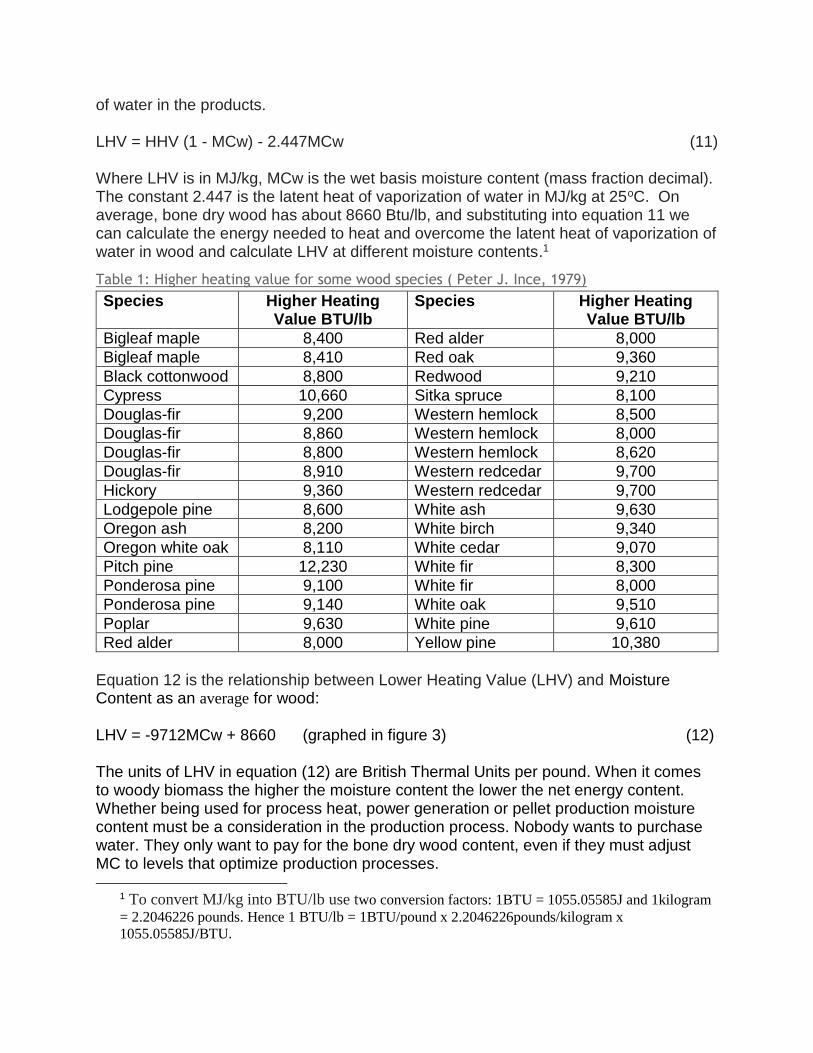
of water in the products. LHV = HHV (1 - MCw) - 2.447MCw (11) Where LHV is in MJ/kg, MCw is the wet basis moisture content (mass fraction decimal). The constant 2.447 is the latent heat of vaporization of water in MJ/kg at 25oC. On average, bone dry wood has about 8660 Btu/lb, and substituting into equation 11 we can calculate the energy needed to heat and overcome the latent heat of vaporization of water in wood and calculate LHV at different moisture contents.1

Table 1: Higher heating value for some wood species ( Peter J. Ince, 1979)

Species Higher Heating Value BTU/lb

Species Higher Heating Value BTU/lb

Bigleaf maple 8,400 Red alder 8,000

Bigleaf maple 8,410 Red oak 9,360

Black cottonwood 8,800 Redwood 9,210

Cypress 10,660 Sitka spruce 8,100

Douglas-fir 9,200 Western hemlock 8,500

Douglas-fir 8,860 Western hemlock 8,000

Douglas-fir 8,800 Western hemlock 8,620

Douglas-fir 8,910 Western redcedar 9,700

Hickory 9,360 Western redcedar 9,700

Lodgepole pine 8,600 White ash 9,630

Oregon ash 8,200 White birch 9,340

Oregon white oak 8,110 White cedar 9,070

Pitch pine 12,230 White fir 8,300

Ponderosa pine 9,100 White fir 8,000

Ponderosa pine 9,140 White oak 9,510

Poplar 9,630 White pine 9,610

Red alder 8,000 Yellow pine 10,380

Equation 12 is the relationship between Lower Heating Value (LHV) and Moisture Content as an average for wood: LHV = -9712MCw + 8660 (graphed in figure 3) (12) The units of LHV in equation (12) are British Thermal Units per pound. When it comes to woody biomass the higher the moisture content the lower the net energy content. Whether being used for process heat, power generation or pellet production moisture content must be a consideration in the production process. Nobody wants to purchase water. They only want to pay for the bone dry wood content, even if they must adjust MC to levels that optimize production processes.

1 To convert MJ/kg into BTU/lb use two conversion factors: 1BTU = 1055.05585J and 1kilogram

= 2.2046226 pounds. Hence 1 BTU/lb = 1BTU/pound x 2.2046226pounds/kilogram x

1055.05585J/BTU.

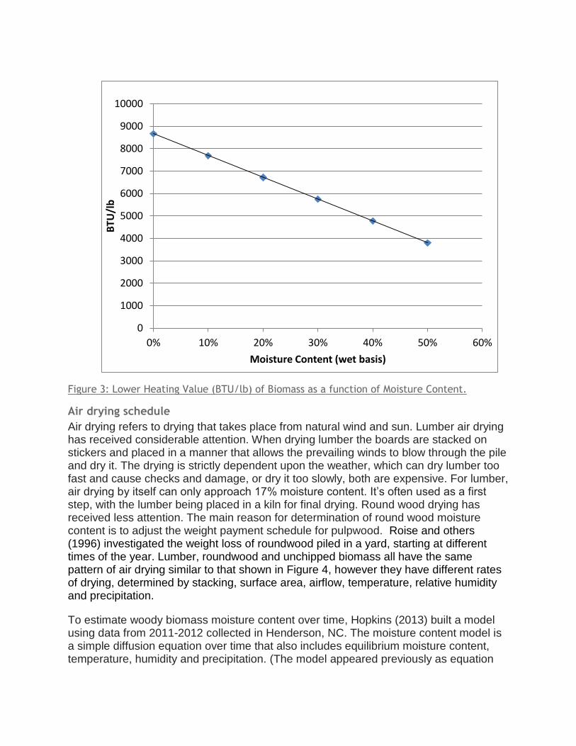
Figure 3: Lower Heating Value (BTU/lb) of Biomass as a function of Moisture Content.

Air drying schedule

Air drying refers to drying that takes place from natural wind and sun. Lumber air drying has received considerable attention. When drying lumber the boards are stacked on stickers and placed in a manner that allows the prevailing winds to blow through the pile and dry it. The drying is strictly dependent upon the weather, which can dry lumber too fast and cause checks and damage, or dry it too slowly, both are expensive. For lumber, air drying by itself can only approach 17% moisture content. It’s often used as a first step, with the lumber being placed in a kiln for final drying. Round wood drying has received less attention. The main reason for determination of round wood moisture content is to adjust the weight payment schedule for pulpwood. Roise and others (1996) investigated the weight loss of roundwood piled in a yard, starting at different times of the year. Lumber, roundwood and unchipped biomass all have the same pattern of air drying similar to that shown in Figure 4, however they have different rates of drying, determined by stacking, surface area, airflow, temperature, relative humidity and precipitation.

To estimate woody biomass moisture content over time, Hopkins (2013) built a model using data from 2011-2012 collected in Henderson, NC. The moisture content model is a simple diffusion equation over time that also includes equilibrium moisture content, temperature, humidity and precipitation. (The model appeared previously as equation

0

1000

2000

3000

4000

5000

6000

7000

8000

9000

10000

0% 10% 20% 30% 40% 50% 60%

BTU

/lb

Moisture Content (wet basis)

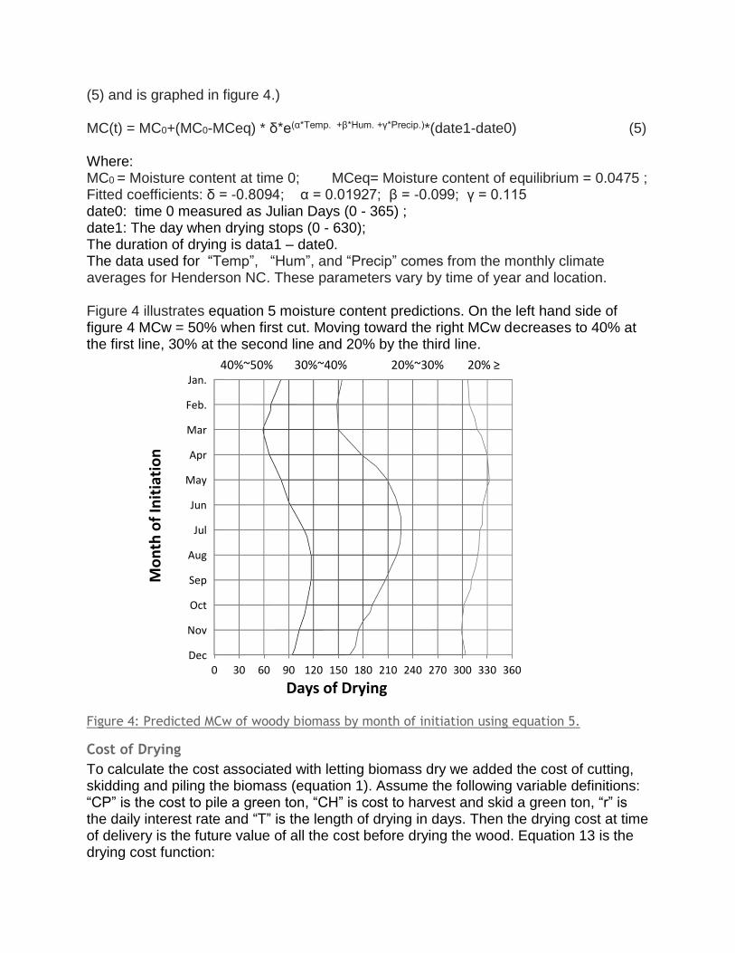
(5) and is graphed in figure 4.) MC(t) = MC0+(MC0-MCeq) * δ*e(α*Temp. +β*Hum. +γ*Precip.)*(date1-date0) (5) Where: MC0 = Moisture content at time 0; MCeq= Moisture content of equilibrium = 0.0475 ; Fitted coefficients: δ = -0.8094; α = 0.01927; β = -0.099; γ = 0.115 date0: time 0 measured as Julian Days (0 - 365) ; date1: The day when drying stops (0 - 630); The duration of drying is data1 – date0. The data used for “Temp”, “Hum”, and “Precip” comes from the monthly climate averages for Henderson NC. These parameters vary by time of year and location. Figure 4 illustrates equation 5 moisture content predictions. On the left hand side of figure 4 MCw = 50% when first cut. Moving toward the right MCw decreases to 40% at the first line, 30% at the second line and 20% by the third line.

Figure 4: Predicted MCw of woody biomass by month of initiation using equation 5.

Cost of Drying

To calculate the cost associated with letting biomass dry we added the cost of cutting, skidding and piling the biomass (equation 1). Assume the following variable definitions: “CP” is the cost to pile a green ton, “CH” is cost to harvest and skid a green ton, “r” is the daily interest rate and “T” is the length of drying in days. Then the drying cost at time of delivery is the future value of all the cost before drying the wood. Equation 13 is the drying cost function:

Jan.

Feb.

Mar

Apr

May

Jun

Jul

Aug

Sep

Oct

Nov

Dec0 30 60 90 120 150 180 210 240 270 300 330 360

Mo

nth

of

Init

iati

on

Days of Drying

40%~50% 30%~40% 20% ≥20%~30%

Drying cost ($/ton) = (CP+ CH)* (1 + r) T (13)

The cost associated with returning to the site for chipping and loading is discussed later, but suffice to say for now, that return to site cost is not compounded into the future.

Energy / Wood Transportation by Chip Vans (equation 7)

The commodity being transported can be considered either wood or energy, and which

perspective will determine the delivered price. We know that, moisture content will affect the

gross weight of wood. For our calculations we assume a 120 yd3 chip van and a maximum

payload weight of 25 tons. These limits vary by equipment and weight limits, but are used as an

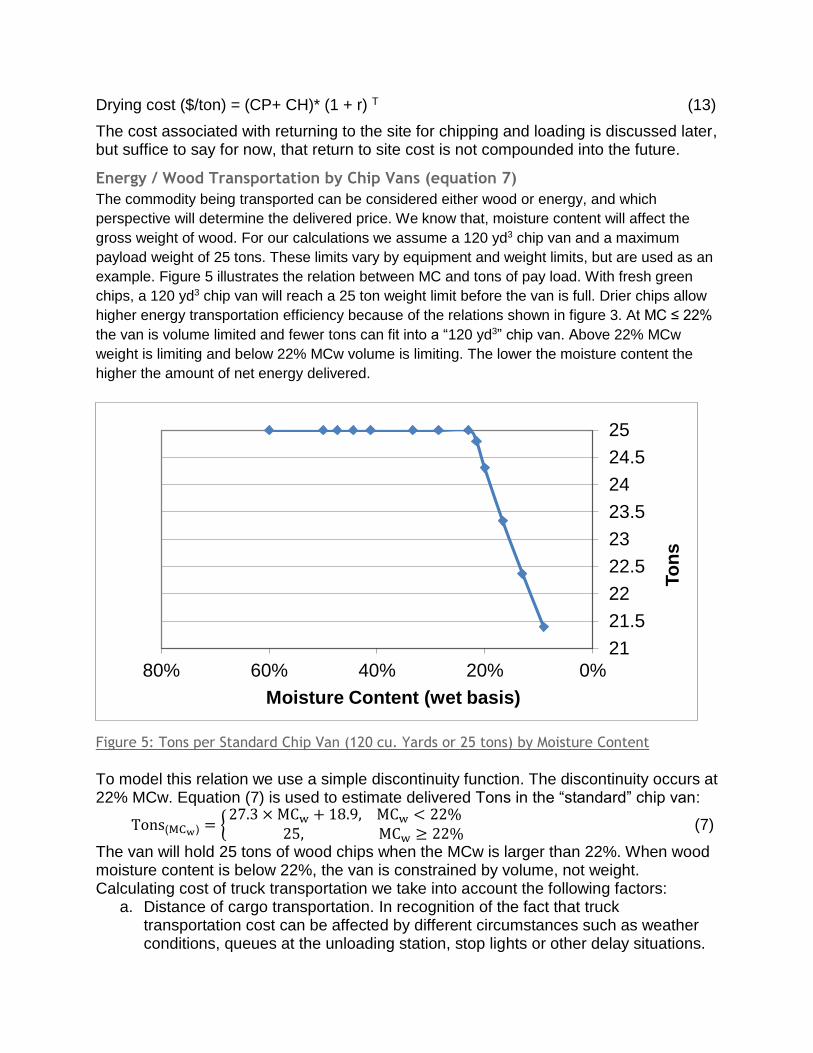
example. Figure 5 illustrates the relation between MC and tons of pay load. With fresh green

chips, a 120 yd3 chip van will reach a 25 ton weight limit before the van is full. Drier chips allow

higher energy transportation efficiency because of the relations shown in figure 3. At MC ≤ 22%

the van is volume limited and fewer tons can fit into a “120 yd3” chip van. Above 22% MCw

weight is limiting and below 22% MCw volume is limiting. The lower the moisture content the

higher the amount of net energy delivered.

Figure 5: Tons per Standard Chip Van (120 cu. Yards or 25 tons) by Moisture Content

To model this relation we use a simple discontinuity function. The discontinuity occurs at 22% MCw. Equation (7) is used to estimate delivered Tons in the “standard” chip van:

Tons(MCw) = {27.3 × MCw + 18.9, MCw < 22% 25, MCw ≥ 22%

(7)

The van will hold 25 tons of wood chips when the MCw is larger than 22%. When wood moisture content is below 22%, the van is constrained by volume, not weight. Calculating cost of truck transportation we take into account the following factors:

a. Distance of cargo transportation. In recognition of the fact that truck transportation cost can be affected by different circumstances such as weather conditions, queues at the unloading station, stop lights or other delay situations.

21

21.5

22

22.5

23

23.5

24

24.5

25

0%20%40%60%80%To

ns

Moisture Content (wet basis)

b. Cost of other work such as chipping, loading and unloading is included in equation 1.

In the model, a simple cost per loaded mile function is used: CT = Cvan * Distance (8) Cvan: Cost per loaded mile of transporting a chip van.

Delivered Price as a function of Net Energy Content a function of Moisture Content

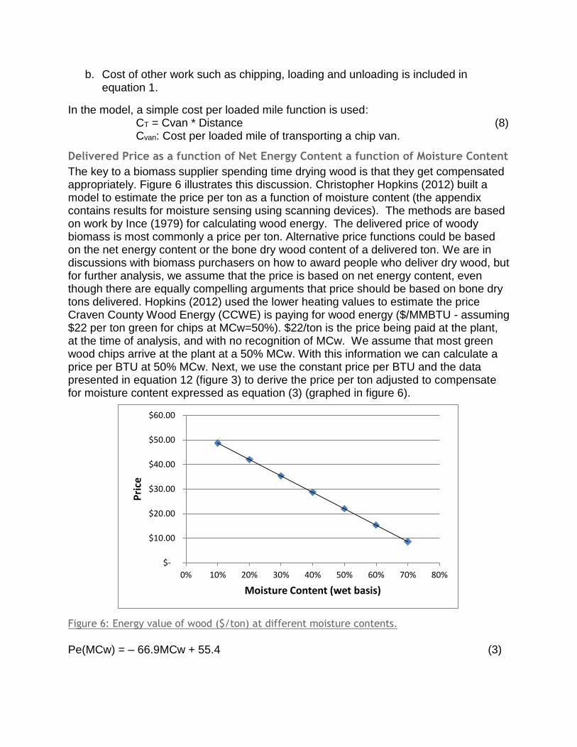
The key to a biomass supplier spending time drying wood is that they get compensated appropriately. Figure 6 illustrates this discussion. Christopher Hopkins (2012) built a model to estimate the price per ton as a function of moisture content (the appendix contains results for moisture sensing using scanning devices). The methods are based on work by Ince (1979) for calculating wood energy. The delivered price of woody biomass is most commonly a price per ton. Alternative price functions could be based on the net energy content or the bone dry wood content of a delivered ton. We are in discussions with biomass purchasers on how to award people who deliver dry wood, but for further analysis, we assume that the price is based on net energy content, even though there are equally compelling arguments that price should be based on bone dry tons delivered. Hopkins (2012) used the lower heating values to estimate the price Craven County Wood Energy (CCWE) is paying for wood energy ($/MMBTU - assuming $22 per ton green for chips at MCw=50%). $22/ton is the price being paid at the plant, at the time of analysis, and with no recognition of MCw. We assume that most green wood chips arrive at the plant at a 50% MCw. With this information we can calculate a price per BTU at 50% MCw. Next, we use the constant price per BTU and the data presented in equation 12 (figure 3) to derive the price per ton adjusted to compensate for moisture content expressed as equation (3) (graphed in figure 6).

Figure 6: Energy value of wood ($/ton) at different moisture contents.

Pe(MCw) = – 66.9MCw + 55.4 (3)

$-

$10.00

$20.00

$30.00

$40.00

$50.00

$60.00

0% 10% 20% 30% 40% 50% 60% 70% 80%

Pri

ce

Moisture Content (wet basis)

Net Revenue maximization as a function of drying time

Now we test the model presented in equations 1-8. Remember that the formulation integrates all the operational cost of getting a van full of biomass from the field to the plant as a function of moisture content:

Analytical results

Given the model defined above the analysis finds the drying time needed to maximize net return associated with delivering a ton of biomass to a purchaser. We did the analysis starting at the first day of each month of the year.

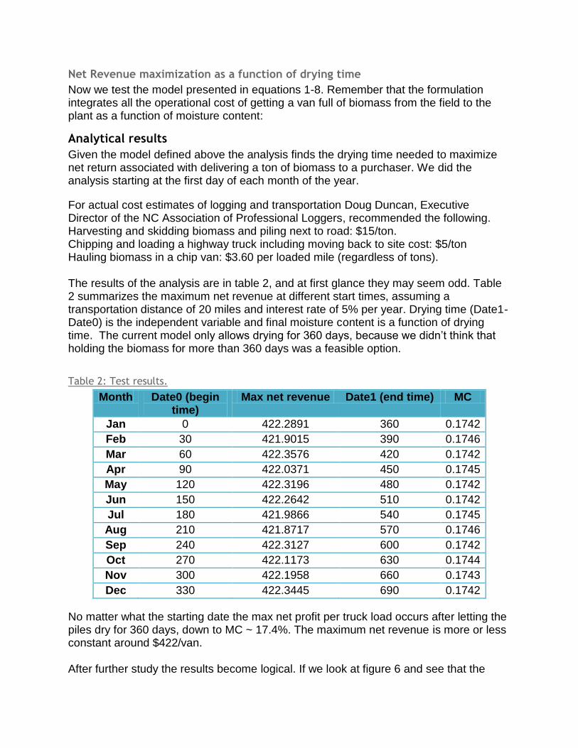
For actual cost estimates of logging and transportation Doug Duncan, Executive Director of the NC Association of Professional Loggers, recommended the following. Harvesting and skidding biomass and piling next to road: $15/ton. Chipping and loading a highway truck including moving back to site cost: $5/ton Hauling biomass in a chip van: $3.60 per loaded mile (regardless of tons). The results of the analysis are in table 2, and at first glance they may seem odd. Table 2 summarizes the maximum net revenue at different start times, assuming a transportation distance of 20 miles and interest rate of 5% per year. Drying time (Date1-Date0) is the independent variable and final moisture content is a function of drying time. The current model only allows drying for 360 days, because we didn’t think that holding the biomass for more than 360 days was a feasible option.

Table 2: Test results.

Month Date0 (begin time)

Max net revenue Date1 (end time) MC

Jan 0 422.2891 360 0.1742

Feb 30 421.9015 390 0.1746

Mar 60 422.3576 420 0.1742

Apr 90 422.0371 450 0.1745

May 120 422.3196 480 0.1742

Jun 150 422.2642 510 0.1742

Jul 180 421.9866 540 0.1745

Aug 210 421.8717 570 0.1746

Sep 240 422.3127 600 0.1742

Oct 270 422.1173 630 0.1744

Nov 300 422.1958 660 0.1743

Dec 330 422.3445 690 0.1742

No matter what the starting date the max net profit per truck load occurs after letting the piles dry for 360 days, down to MC ~ 17.4%. The maximum net revenue is more or less constant around $422/van. After further study the results become logical. If we look at figure 6 and see that the

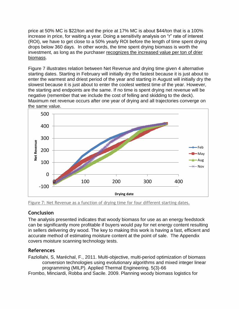
price at 50% MC is $22/ton and the price at 17% MC is about $44/ton that is a 100% increase in price, for waiting a year. Doing a sensitivity analysis on “r” rate of interest (ROI), we have to get close to a 50% yearly ROI before the length of time spent drying drops below 360 days. In other words, the time spent drying biomass is worth the investment, as long as the purchaser recognizes the increased value per ton of drier biomass. Figure 7 illustrates relation between Net Revenue and drying time given 4 alternative starting dates. Starting in February will initially dry the fastest because it is just about to enter the warmest and driest period of the year and starting in August will initially dry the slowest because it is just about to enter the coolest wettest time of the year. However, the starting and endpoints are the same. If no time is spent drying net revenue will be negative (remember that we include the cost of felling and skidding to the deck). Maximum net revenue occurs after one year of drying and all trajectories converge on the same value.

Figure 7: Net Revenue as a function of drying time for four different starting dates.

Conclusion

The analysis presented indicates that woody biomass for use as an energy feedstock can be significantly more profitable if buyers would pay for net energy content resulting in sellers delivering dry wood. The key to making this work is having a fast, efficient and accurate method of estimating moisture content at the point of sale. The Appendix covers moisture scanning technology tests.

References

Fazlollahi, S, Maréchal, F., 2011. Multi-objective, multi-period optimization of biomass conversion technologies using evolutionary algorithms and mixed integer linear programming (MILP). Applied Thermal Engineering. 5(3)-66

Frombo, Minciardi, Robba and Sacile. 2009. Planning woody biomass logistics for

-100

0

100

200

300

400

500

0 100 200 300 400

Ne

t R

eve

nu

e

Drying date

Feb

May

Aug

Nov

energy production: A strategic decision model. Biomass and Bioenergy, Vol.33(3), pp. 372-383

Hopkins, C.. 2013. In-Field Drying Improves Woody Biomass Energy. Presented at the NCSU Graduate Research Symposium, March 19, 2013. Mc Kimmon Center, Raleigh, North Carolina.

Ince, P, J. 1979. How to estimate recoverable heat energy in wood or bark fuels. Forest Products Laboratory. General Technical Report FPL 29.

Navarrete, E. 2012, "Modeling optimal pine stands harvest under stochastic wood stock and price in Chile", Forest Policy and Economics, vol. 15, pp. 54-59.

Mobini, M., Sowlati, T. & Sokhansanj, S. 2011, "Forest biomass supply logistics for a power plant using the discrete-event simulation approach", Applied Energy, vol. 88, no. 4, pp. 1241-1250.

Payne, J. 2012. On Biomass Energy Consumption and Real Output in the US. Energy Sources Part B: Economics, Planning & Policy [serial online]. January 2011;6(1):47-52. Available from: Computers & Applied Sciences Complete, Ipswich, MA.

Ravula, Grisso, Cundiff. 2007. Cotton Logistics as a model for a biomass transportation system. Biomass and Bioenergy, Vol. 32(4), pp. 314-325

Roise, J.P., Whitlow P.E., Deal, E.L., 1996. Equations for predicting weight loss in stored pulpwood for North Carolina and Virginia. Forest products Society. 49(1):77-81

Appendix: Moisture sensing and measurement in Wood Chips

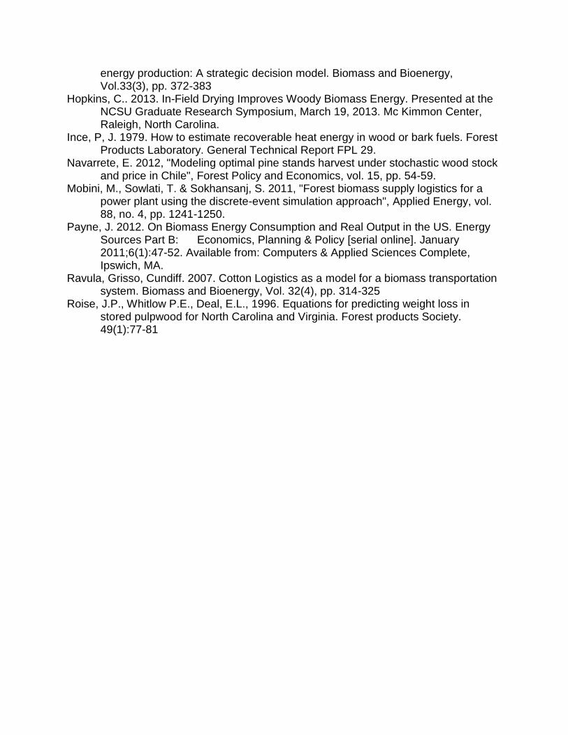
The proposition that air drying wood will result in increased revenue and decreased costs for biomass suppliers depend on the ability to measure moisture content accurately at the point of delivery. If we cannot measure moisture content there is no way for the suppliers to get reimbursed for efforts associated with drying wood. To be operational the measurement of moisture must coincide with the measurement of weight. Weight is generally measured as the difference between loaded truck weight and tare (empty) weight on scales at the point of sale. Once the loaded trucks are weighted, they proceed to the dump which lifts the whole truck up at an angle and the biomass flows out into a hopper (figure A1). Then the empty truck gets weighted again, giving the tare weight. During this process the moisture content needs to be measured. Using moisture scanning technologies we can sample each truck load at the dump, giving an estimate of moisture content. Our research is investigating the application of scanning technology to estimate MCw at point of sale.

Figure A1: The chip dump at Craven Wood Energy, New Burn, NC

In our tests we used in-line moisture sensing technologies from 3 manufacturers: Moisttech (near IR unit equipped with proximity sensor); ProcessSensors (near IR); and MALCAM (microwave). The goal was to perform an unbiased comparison of these wood moisture sensors and gain an appreciation of how to integrate into wood procurement systems at plants. We also needed to determine a protocol for calibrating each machine for possible deployment. For calibration and model development we took 30 samples of pine, hardwood, mixes, microchips, full size chips of variable moisture contents and ran each sample through each machine measuring reflectance (infrared) or transmission (microwave). Fresh samples and partially air dried samples were passed over the near IR moisture meters and dropped into the bin of the MALCAM unit. A sample would take about 20 seconds to be measured by all three machines. Following the scanners the samples were oven dried to determine actual moisture content on a wet basis (MCw). Oven dried samples (0.5-1 kg) were compared to each moisture sensing system.

Results from moisture content scaning

Figures A2 – A4 show the results from the three machines. It appears that MALCAM has the greatest precision, with Process Sensors being next. The accuracy and bias is thought to be the same for each system. We are currently testing the deployment these units in the field at Coastal Carolina Power and Craven County Wood Energy. In the summer of 2013, we are still in the process of securely mounting, calibrating, and testing at the dump site.

Figure A2: Best fit model associated with the MALCAM microwave result

y = 0.3114ln(x) - 0.6643R² = 0.9362

0 10 20 30 40 50

0%

10%

20%

30%

40%

50%

60%

Received Device Readout

MC

wet

bas

is

Malcam 1045

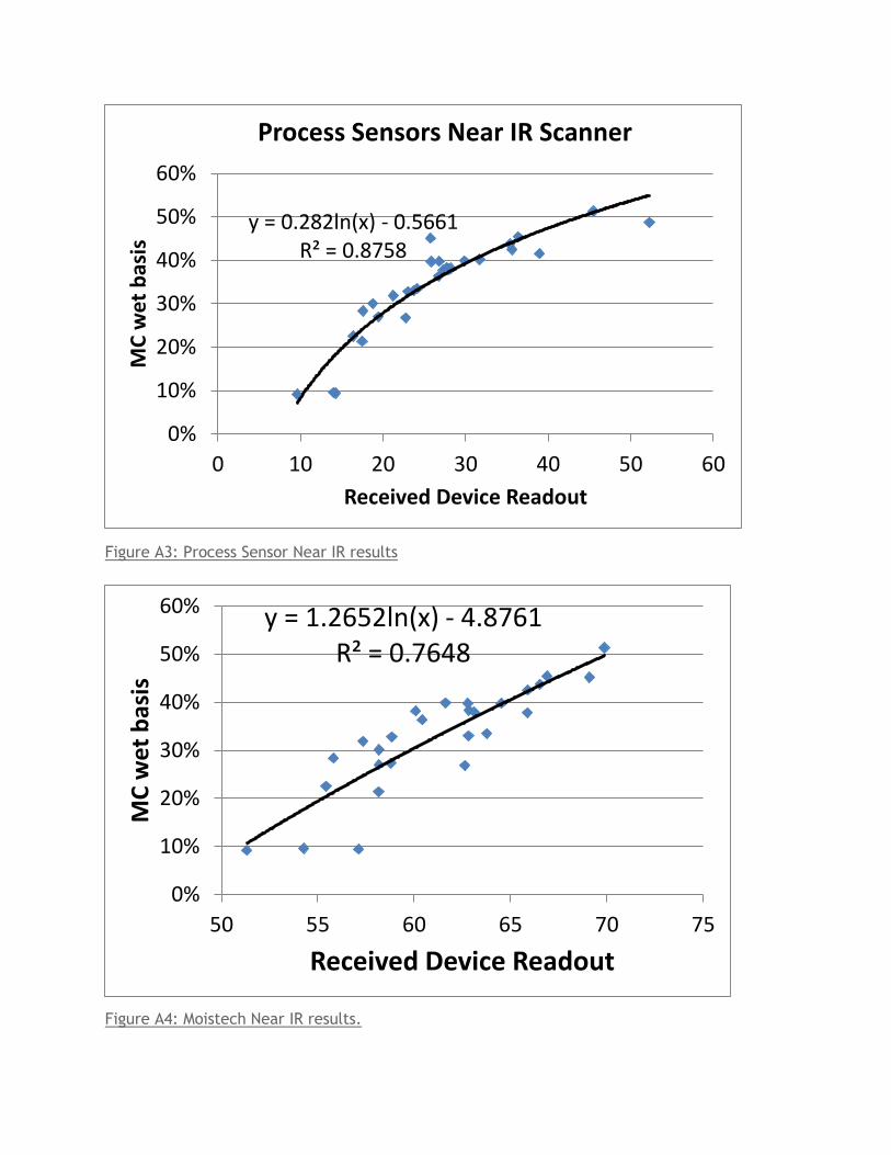
Figure A3: Process Sensor Near IR results

Figure A4: Moistech Near IR results.

y = 0.282ln(x) - 0.5661R² = 0.8758

0%

10%

20%

30%

40%

50%

60%

0 10 20 30 40 50 60

MC

wet

bas

is

Received Device Readout

Process Sensors Near IR Scanner

y = 1.2652ln(x) - 4.8761R² = 0.7648

0%

10%

20%

30%

40%

50%

60%

50 55 60 65 70 75

MC

wet

bas

is

Received Device Readout