Balancing Accuracy and Parsimony in Genetic Programming 1995... · Balancing Accuracy and Parsimony in Genetic Programming Byoung-Tak Zhang Heinz Miihlenbein German National Research

Balancing Accuracy and Parsimony in Genetic Programming

Byoung-Tak Zhang Heinz Miihlenbein German National Research Center for Computer Science (GMD) Schloss Birlinghoven Schloss Birlinghoven D-53754 Sankt Augustin Germany Germany [email protected] [email protected]

German National Research Center for Computer Science (GMD)

D-53754 Sankt Augustin

Abstract Genetic programming is distinguished from other evolutionary algorithms in that it uses tree representations of variable size instead of linear strings of fixed length. The flexible representation scheme is very important because it allows the underlying structure of the data to be discovered automatically. One primary difficulty, however, is that the solutions may grow too bigwithout any improvement oftheir generalization ability. In this article we investigate the fundamental relationship between the performance and complexity of the evolved structures. The essence of the parsimony problem is demonstrated empirically by analyzing error landscapes of programs evolved for neural network synthesis. We consider genetic programming as a statistical inference problem and apply the Bayesian model- comparison framework to introduce a class of fitness functions with error and complexity terms. An adaptive learning method is then presented that automatically balances the model-complexity factor to evolve parsimonious programs without losing the diversity of the population needed for achieving the desired training accuracy. The effectiveness of this approach is empirically shown on the induction of sigma-pi neural networks for solving a real-world medical diagnosis problem as well as benchmark tasks.

machine learning, tree induction, genetic programming, minimum description length principle, Bayesian model comparison, evolving neural networks

Keywords

1. Introduction

Machine learning has been a major research area since the birth of artificial intelligence as a discipline (Samuel, 1963; Winston, 1975). Learning is not only an inalienable component of human intelligence, but it also plays an important role in constructing high-performance application systems (Carbonell, 1990). Recently, Koza introduced a new learning paradigm, called genetic programming (Koza, 1992a), which extends conventional evolutionary algorithms (Back & Schwefel, 1993; Goldberg, 1989; Muhlenbein & Schlierkamp-Voosen, 1993) in that the structures undergoing adaptation are hierarchical computer programs instead of bitstrings. Genetic programming has been successfully applied to learn computer programs for solving many interesting problems in artificial intelligence and artificial life (Koza, 1992a; Koza, 1994; Kinnear, 1994a).

As with other evolutionary algorithms, genetic programming starts with a population of randomly generated individuals. Each individual is a program that, when executed, is the candidate solution to the problem. Selection and crossover operators are used to produce

@ 1995 The Massachusetts Institute of Technology Evolutionary Computation 3(1): 17-38

Byoung-Tak Zhang and Heinz Miihlenbein

increasingly fit populations of computer programs. While most evolutionary algorithms are based on chromosomes of fixed length, genetic programming uses hierarchical structures, that is, trees of variable size and shape. In the most general case, the programs can be LISP S-expressions representing a game-playing strategy, a set of production rules, a decision tree, or a neural network. The structured representation scheme is particularly well suited to problems in which the regularity of the underlying process must be discovered from observed data.

One problem with the flexible size representation in genetic programming is tha t the space and time requirements of the structures may become too great. Larger programs take more execution time than smaller ones; when all the elementary operations take the same time, the total execution time is proportional to the size of the program. In some applications such as synthesis of logic circuits or neural networks, one may wish to implement the final solutions in hardware. In this case, larger solutions also result in higher implementation costs. In addition, as their size increases, the programs frequently become hopelessly opaque to human understanding (Kinnear, 1993). One approach to dealing with this problem is to define and reuse submodules. Koza suggests defining potentially useful subroutines called automatically defined finctions (ADFs) during a run (Koza, 1992b). Genetic programming with automatic function definition significantly reduces the average structural complexity of the solutions and the computational effort as compared to genetic programming without automatic function definition (Koza, 1993).

However, even with reusable submodules the program size may still grow without bound if the training data is noisy or incomplete. Empirical studies report that, when their training accuracy is comparable, smaller solutions usually demonstrate better generalization performance than larger solutions. Tackett, for instance, observes in his pattern classification experiments that a high degree of correlation exists between tree size and performance: “among the set of ‘pretty good’ solutions, the smallest within the set usually achieved the highest performance” (Tackett, 1993, p. 309). He also observed that, as the size and complexity of trees grew, a point was eventually reached in most runs where performance dropped. H e suggests that for an open-ended exploration of problem space, parsimony may be an important factor not for aesthetic reasons or ease of analysis, but because there seems to be a bound on the appropriate size of solution trees for a given problem. Kinnear reports that as his programs grew, it became less and less likely for them to be general Wnnear, 1993). He questions whether there are other problems for which generalization is inversely proportional to the program size.

In this article we show that the problem of parsimony is ubiquitous in genetic programming from a theoretical point of view. In Section 2, we use the results from the statistics literature to shed light on the fundamental relationship between accuracy and parsimony in genetic programming. In Section 3, the essence of the problem is demonstrated empirically when we analyze error landscapes of programs evolved for neural network synthesis. In Section 4, a Bayesian model-comparison method is used to develop a framework in which a class of fitness measures is introduced for dealing with problems of parsimony. We then describe an adaptive technique for putting this fitness function into practice. It automatically balances the ratio of training accuracy to solution complexity without losing the population diversity needed to achieve a specified training accuracy. The effectiveness of the method is shown in Section 6, where simulation results are presented demonstrating the induction of neural networks using noisy training data. In Section 7 we discuss the relationship of this work with other tree-based machine learning methods. Section 8 concludes by summarizing the results and implications of this work.

18 Evolutionary Computation Volume 3, Number 1

W l I

Balancing Accuracy and Parsimony

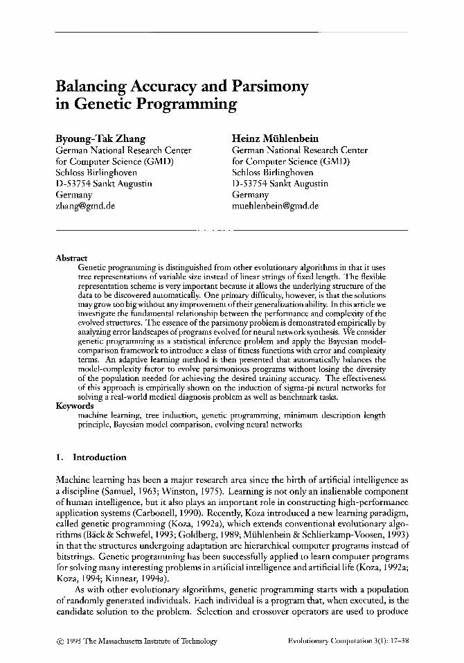
Figure 1. has a local

Tree representation of a sigma-pi neural network with six inputs and one receptive field.

output. Each unit

2. Genetic Programming and the Bias-Variance Problem

Many seemingly different problems in artificial intelligence and artificial life can be viewed as the problem of discovering a computer program that produces some desired output for particular inputs. For instance, in visual pattern-recognition applications the input of a program A is a vector x of features from a segmented image and each component yk of the output vector y may represent the probability that the image belongs to category k.

The process of solving these problems can be formulated as a search for a highly fit computer program, Abest, in the whole space of possible computer programs A:

The evolutionary approach differs from most other search techniques in that it makes a parallel search simultaneously involving hundreds or thousands of points in the search space. Genetic programming starts with an initial population A of randomly generated computer programs composed of elementary functions and terminals chosen by the domain expert. The elementary functions may be arithmetic operations, logical functions, standard programming operations, or domain-specific functions.

In the synthesis of sigma-pi neural networks (Zhang & Muhlenbein, 1994), for instance, the terminal set X consists of n input variables:

x = {x1,x2,. . . ,Xn} (4

u = {S ,P} . (3)

and the elementary function set U contains sigma (S) and pi (P) units:

An instance of the program consisting of the above elementary functions, that is, a sigma-pi neural network, is shown in Figure 1. This program consists of three S units and two P units in an embedded list structure

where Sj and Pi are realizations of a sigma and pi unit at ith node, respectively. Notice that although the number of primitive functions and terminals is finite, any arbitrarily large programs can be generated by recursive use of them.

Each unit, Si or Pi, has its own receptive field R(i), the set of incoming connections from other units or from external inputs.’ Each input connection is associated with a weight

1 The bias or threshold can be treated as a weight connected to a special unit whose activation value is always 1. Thus, in the following discussion we consider the bias as just another input to the unit.

Evolutionary Computation Volume 3 , Number 1 19


value, wf, denoting the strength of the connection fromj to i. Neuron types differ in their computation of activation values. Sigma units, S;, compute the weighted sum of these inputs

{ :: if CJERQ w&Y! > yj = Sj(X) = otherwise,

while pi units, Pi, compute the product of their weighted inputs

(5)

The quality of each computer program in the population is measured in terms of how well it performs in the particular problem environment. T h s measure is called the fitness measure. Typically, each computer program in the population is run over a number of different input-output cases so that its fitness is measured as a sum or an average over their errors. The set of such cases is called the training set, D:

D = { ( x E , Y c ) E (7)

where x, E X and y, E Y. The domain X and the range Y are defined by the application. The training set is assumed to be generated from an unknown relationshipf satisfymg

yc =i’ (xE>. (8)

Iff is stochastic, it is further assumed that the relationf can be described by a probability density function defined over the space X x Y :

where Pf(x) defines the regon of interest in the input space, and Pf(y I x) describes the statistical relation between the inputs and the outputs.

Given this, the goal of genetic programming is formulated as finding a program A E A that computes the best approximationfA(x) tof based on the training set D. This is a typical learning-from-examples problem. In order to choose the best available approximation, we measure the discrepancy, or loss, Q(y,fA(x)) between the target response y to a given input x and the actual responsefA(x) provided by the program. The loss function most commonly used is the sum of squared errors:

Now that the similarity of genetic programming and learning from examples has been established, we can analyze the process of genetic programming by means of the techniques developed in statistical inference. The genetic-programming paradigm uses a training set of fixed size to evolve the programs, but the eventual goal is the minimization of the error over all possible data in the domain. In other words, we try to minimize the average error,

. N

20 Evolutionary Computation Volume 3 , Number 1


constructed on the basis of the training set D of size N , while the eventual goal of learning is to minimize the expected value of the loss

But the joint probability distribution Pf(x,y) = Pf(y I x)Pf(x) is unknown, and the only available information is contained in the training set D. Taking Q(yc,fA(q)) = 0. -fA(x))’, the effectiveness off as a predictor of y, given D and a particular x, is measured by the mean-squared error:

(13)

where E[.] is the expectation operator. Here we used the notationfA(x; 0) instead offA(x) to denote explicitly the dependency of the function fA or the program A on the training data D. Some manipulation of the formula shows that this can be decomposed into two terms (Breiman, Friedman, Olshen, & Stone, 1984; Geman, Bienenstock, & Doursat, 1992):

m y -fA(x; m2 I x, DI.

E[(y-fA(x;D))2 I x,Dl = E[(y-E[Ylxl)21x,~l +(E[ylxl -fA(x;D))’. (14)

Here E[(y - E[y I XI)’ I x, D] does not depend on the data D, nor on the estimatorf. Hence the squared distance to the regression function E[y I x], (E[y I x] -fA(x; D))2 measures in a natural way the effectiveness off as a predictor of y. The mean-squared error off as an estimator of the regression is

(1 5)

where ED represents expectation with respect to the training set D, that is, the average over the ensemble of possible D (for fixed sample size N). This error can again be decomposed into two terms:

E D [(E[y I XI -fA(x;D))2] 7

E D [(E[y I XI -h (x ; D))’] = (ED[fA(x; 011 - E[y I XI)’

-k E D [(fA(x; 0) - ED[fA(x; D)1l2] (16)

In essence, this states that there are two different kinds of errors. One is the error caused when, on the average, fA(x; 0) is different from E[y 1 XI. This type of error is called bias error. The second type of error, variance error, is caused iffA(x; 0) is hghly sensitive to the data and far from the regression E [ y I x] even with small bias or E~[fi(x;D)] = E[y I XI. Thus either bias or variance can contribute to poor performance. Because complex models can reduce bias error more easily (i.e., training error can be very small) than simpler ones but will in general have large variance (i.e., the resulting model is very specific to the data chosen for training), the theory suggests that smaller programs should be preferred to larger ones, regardless of concrete description forms used. In the next section we empirically study this phenomenon by examining the error landscape.

3. Generalization versus Complexity

In an attempt to examine the relationship between accuracy and structural complexity, we analyzed the error landscape of sigma-pi neural networks (Zhang, 1994). Landscape analysis techniques have also been used to characterize the difficulty of the tasks in genetic algorithms



(Manderick, de Weger, & Spiessens 1991) and in genetic programming @nnear, 1994b). We used the parity problem with input size n = 7. We first generated a clean data set DN of size N = z7. A noisy training set DN was then produced from DN by flipping the output value of each example with 5% probability.

Approximately M = 20000 sigma-pi networks of differing size with binary-valued weights were randomly generated. Each network Ai was then trained on the noisy data DN using the error measure

where yc and f ( ~ ; A i ) are the desired and actual output value of the ith network given the input pattern q. The training was performed by a simple hill-climbing method in which a new weight configuration is generated by mutating the existing configuration. After training, the generalization performance E(DN I Ai) of the network was measured on the test set D N

of N clean examples. Two normalized performance measures were then produced for each network:

(18)

(19)

1 T(i) = -Q@N I Ai), N

1 G(i) = EQ(DN I Ail.

The number of weights in each network is used as a complexity measure:

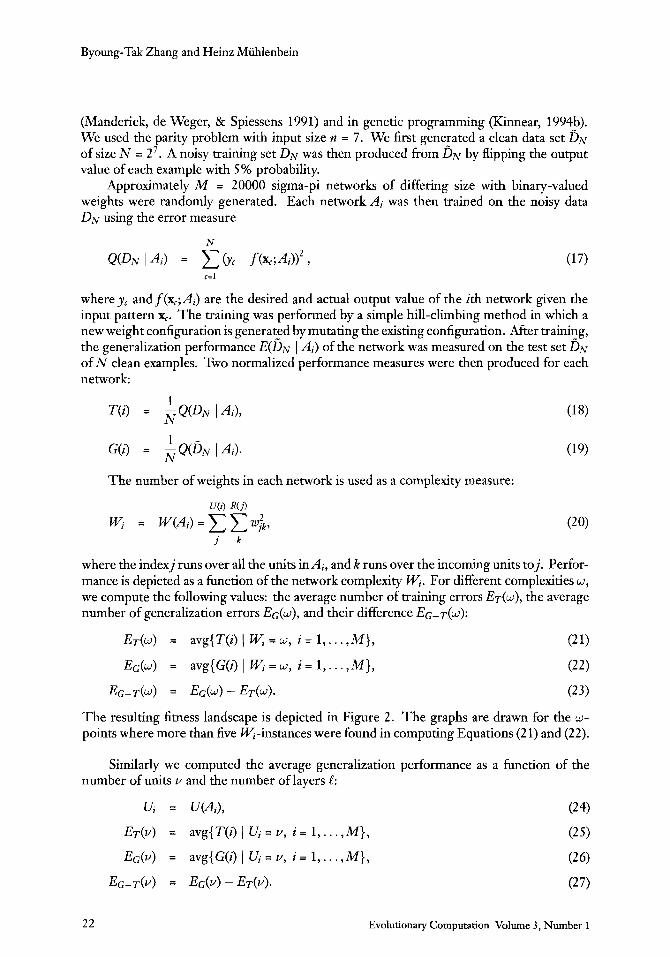
where the indexj runs over all the units in Ai, and k runs over the incoming units toj. Perfor- mance is depicted as a function of the network complexity Wi. For different complexities w, we compute the following values: the average number of training errors ET(w), the average number of generalization errors EG(w), and their difference EG-T(w):

The resulting fitness landscape is depicted in Figure 2. The graphs are drawn for the w- points where more than five Wi-instances were found in computing Equations ( 2 1) and (22) .

Similarly we computed the average generalization performance as a function of the number of units v and the number of layers e:



0 4 -

F ' 0.3. E a

a E @ 0 2 -

5 0.1 - L a

0.0 .

- 0 1 - 0 50 100 150 200 250

O 5 c 0.5

. . . . , . . . , . . . . , . . . . , . . . , I 3 50 100 150 200 250

0 5 -

0 4 -

F :

E :

@ 0 2 -

' 0.3 - m

g 0 1 -

0 .

0.0 - . . . . . . . . . .. . generalization error (G)

-0.1 4

number of weights number of weights

Figure 2. Effect of the number of weights on generalization.

. . . . , , , , , , . . . . , , , , , , . . .

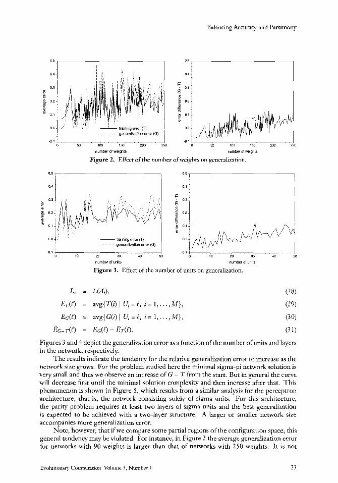
Figures 3 and 4 depict the generalization error as a function of the number of units and layers in the network, respectively.

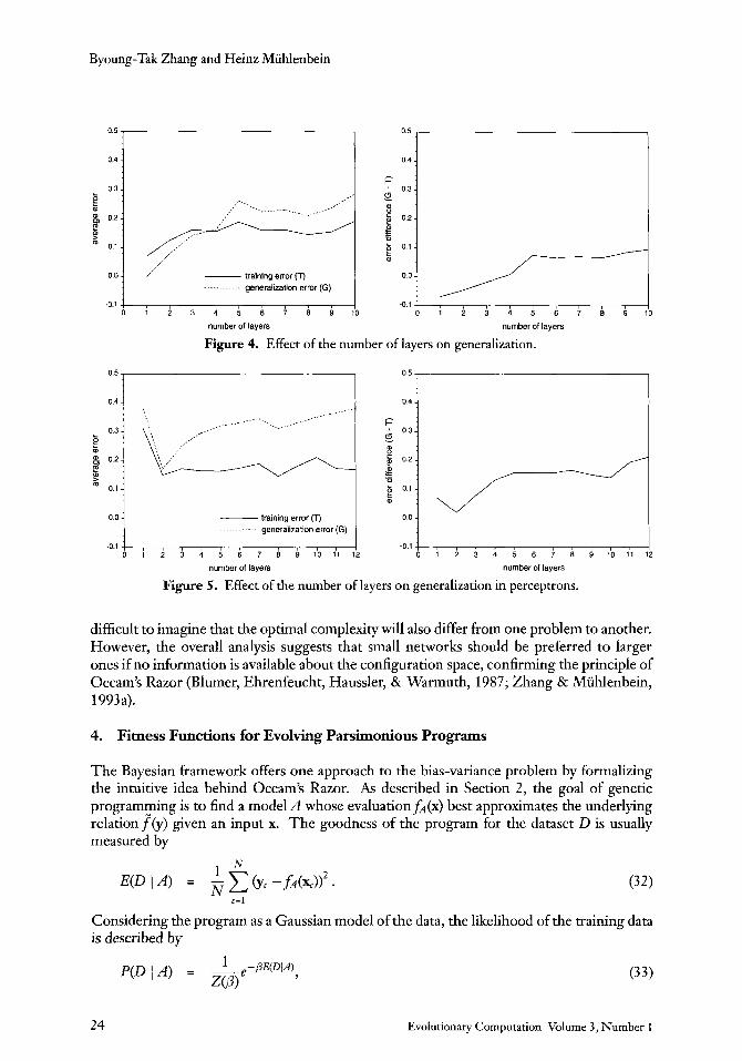
The results indicate the tendency for the relative generalization error to increase as the network size grows. For the problem studied here the minimal sigma-pi network solution is very small and thus we observe an increase of G - T from the start. But in general the curve will decrease first until the minimal solution complexity and then increase after that. This phenomenon is shown in Figure 5, which results from a similar analysis for the perceptron architecture, that is, the network consisting solely of sigma units. For this architecture, the parity problem requires a t least two layers of sigma units and the best generalization is expected to be achieved with a two-layer structure. A larger or smaller network size accompanies more generalization error.

Note, however, that if we compare some partial regions of the configuration space, this general tendency may be violated. For instance, in Figure 2 the average generalization error for networks with 90 weights is larger than that of networks with 250 weights. It is not

I

Evolutionary Computation Volume 3 , Number 1 2 3

Byoung-Tak Zhang and Heinz Muhlenbein

F ' 0.3 I s : $ : E 0.2 -

E 0.1 I

m E

b

0 ' I;,'', , , , , I , , training error (T) . . . . . . . . . . . . generalization error (G)

-0.1 0 1 2 3 4 5 6 7 8 9

number of layers

0.5 -

..._. ...- __-. ___.- . ..-- ... _..._.__ ....- ._ - ____....-

0.4

0.5

0 4 -

F ' 03: s : $ :

/

g 0.2:

0.1 - 5 0.1 I

m

U Z ' 5

b :

0.0 - training error (T) 0.0 -

-0.1 7 , , , , , , , , , , , -0.1;

. . . . . . . . . .. . generalization error (G)

/

, , ~ , , , , , , , ,

0 1 2 3 4 5 6 7 8

number of layers

difficult to imagne that the optimal complexity will also differ from one problem to another. However, the overall analysis suggests that small networks should be preferred to larger ones if no information is available about the configuration space, confirming the principle of Occam's Razor (Blumer, Ehrenfeucht, Haussler, & Warmuth, 1987; Zhang & Miihlenbein, 1993a).

4. Fitness Functions for Evolving Parsimonious Programs

The Bayesian framework offers one approach to the bias-variance problem by formalizing the intuitive idea behind Occam's Razor. As described in Section 2, the goal of genetic programming is to find a model A whose evaluationfA(x) best approximates the underlying relation?(y) given an input x. The goodness of the program for the dataset D is usually measured by

Considering the program as a Gaussian model of the data, the likelihood of the training data is described by



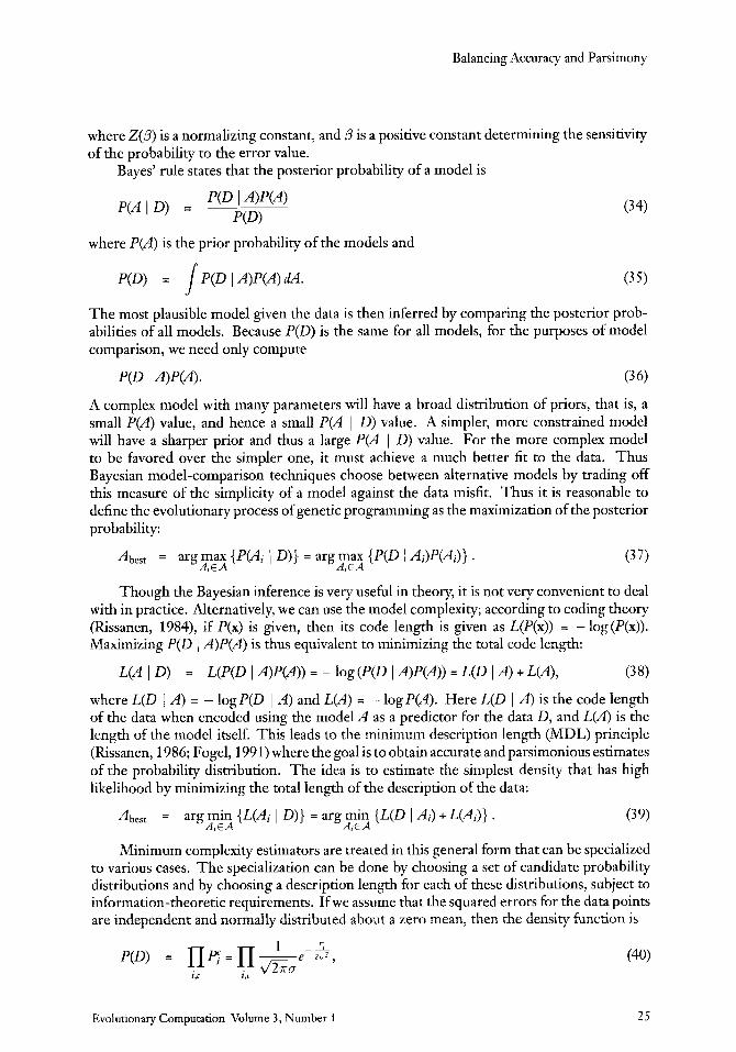
where Z(p) is a normalizing constant, and /3 is a positive constant determining the sensitivity of the probability to the error value.

Bayed rule states that the posterior probability of a model is

where P(A) is the prior probability of the models and

P(D) = 1 P(D I A)P(A) dA. ( 3 5)

The most plausible model given the data is then inferred by comparing the posterior prob- abilities of all models. Because P(D) is the same for all models, for the purposes of model comparison, we need only compute

P(D IA)P(A). ( 3 6)

A complex model with many parameters will have a broad distribution of priors, that is, a small P(A) value, and hence a small P(A I 0) value. A simpler, more constrained model will have a sharper prior and thus a large P(A I 0) value. For the more complex model to be favored over the simpler one, i t must achieve a much better fit to the data. Thus Bayesian model-comparison techniques choose between alternative models by trading off this measure of the simplicity of a model against the data misfit. Thus it is reasonable to define the evolutionary process of genetic programming as the maximization of the posterior probability:

Abest = arg max {P(A; 1 D)} = arg max {P(D 1 A;)P(A;)} . ( 3 7 ) A,Ed A ,EA

Though the Bayesian inference is very useful in theory, it is not very convenient to deal with in practice. Alternatively, we can use the model complexity; according to coding theory (Rissanen, 1984), if P(x) is given, then its code length is given as L(P(x)) = - log(P(x)). Maximizing P(D I A)P(A) is thus equivalent to minimizing the total code length:

L(A I 0) = L(P(D I A)P(A)) = - log (P(D I A)P(A)) = L(D I A) + L(A), ( 3 8)

where L(D I A) = - logP(D I A) and L(A) = - logP(A). Here L(D I A) is the code length of the data when encoded using the model A as a predictor for the data D, and L(A) is the length of the model itself. This leads to the minimum description length (MDL) principle (Rissanen, 1986; Fogel, 1991) where the goal is to obtain accurate and parsimonious estimates of the probability distribution. The idea is to estimate the simplest density that has high likelihood by minimizing the total length of the description of the data:

Abest = arg min {L(A; I D)} = arg min {L(D I A,) + L(A,)}. A,EA A,EA

( 3 9)

Minimum complexity estimators are treated in this general form that can be specialized to various cases. The specialization can be done by choosing a set of candidate probability distributions and by choosing a description length for each of these distributions, subject to information-theoretic requirements. If we assume that the squared errors for the data points are independent and normally distributed about a zero mean, then the density function is


Byoung-Tak Zhang and Heinz Mthlenbein

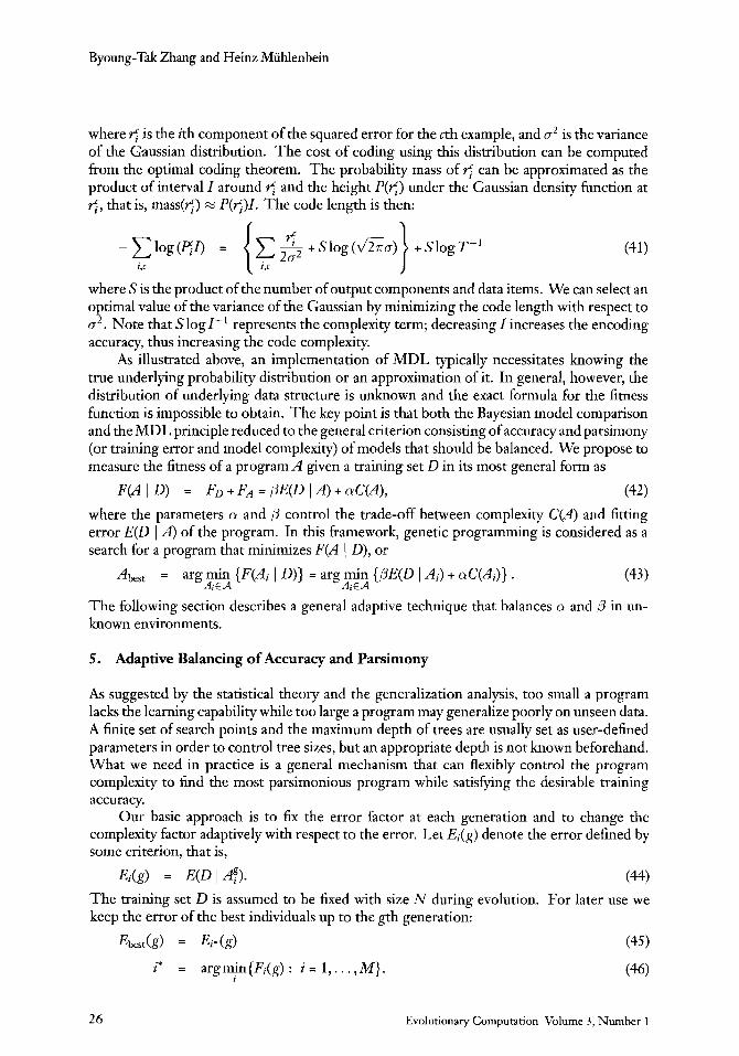
where I$ is the ith component of the squared error for the cth example, and u2 is the variance of the Gaussian distribution. The cost of coding using this distribution can be computed from the optimal coding theorem. The probability mass of < can be approximated as the product of interval I around c and the height P ( c ) under the Gaussian density function a t <, that is, mass(c) M P(c)I. The code length is then:

where S is the product of the number of output components and data items. We can select an optimal value of the variance of the Gaussian by minimizing the code length with respect to u2. Note that S logl-' represents the complexity term; decreasing I increases the encoding accuracy, thus increasing the code complexity.

As illustrated above, an implementation of MDL typically necessitates knowing the true underlying probability distribution or an approximation of it. In general, however, the distribution of underlying data structure is unknown and the exact formula for the fitness function is impossible to obtain. The key point is that both the Bayesian model comparison and the MDL principle reduced to the general criterion consisting of accuracy and parsimony (or training error and model complexity) of models that should be balanced. We propose to measure the fitness of a program A given a training set D in its most general form as

F(A I 0) = Fo +FA = PE(D I A) + aC(A), (42) where the parameters (Y and P control the trade-off between complexity C(A) and fitting error E(D I A ) of the program. In this framework, genetic programming is considered as a search for a program that minimizes F(A 1 D), or

(43) Abest = arg min {F(A; I D)} = arg min {PE(D I A,) + (rC(A,)} . A , € d A , € A

The following section describes a general adaptive technique that balances (Y and 0 in unknown environments.

5. Adaptive Balancing of Accuracy and Parsimony

As suggested by the statistical theory and the generalization analysis, too small a program lacks the learning capability while too large a program may generalize poorly on unseen data. A finite set of search points and the maximum depth of trees are usually set as user-defined parameters in order to control tree sizes, but an appropriate depth is not known beforehand. What we need in practice is a general mechanism that can flexibly control the program complexity to find the most parsimonious program while satisfymg the desirable training accuracy.

Our basic approach is to fix the error factor at each generation and to change the complexity factor adaptively with respect to the error. Let Ei(g) denote the error defined by some criterion, that is,

Ei(g) = E(D I A?). (4.4) The training set D is assumed to be fixed with size N during evolution. For later use we keep the error of the best individuals up to the gth generation:

Ebest<g) = Ei*(g) (45)

i* = argmjn{Fi(g) I : i = 1,. . . ,M} . (46)



Here Fi(g) is the total fitness value of the ith individual at generationg used for reproduction of the next population.

Let Ci(g) be the complexity value of ith individual in gth population. The complexity of the program may be defined in several ways. For instance, in the case of neural-network synthesis, shallow networks with a small number of units and weights should be preferred to deep structures with a large number of units and weights. The total complexity of the network can thus be defined as a linear sum:

ci(g) = C(AF) = W(A$) + U(Af> + L(AP), (47)

where W(Af), U(Af), and L(A:) denote the number of weights, units, and layers respectively. More generally, complexity is defined in terms of a number of factors K,, which are weighted according to the requirements of the application' :

At the end of each generation g we also keep the complexity of the best individual:

cbest(g) = ci*<g) i' = argmin{Fi(g) : i = 1,. . . , M } .

2

(49)

(50)

Based on Cbest(g), the size of the best individual at the next generation is estimated as

t b e s t ( g + 1) = cbest(g) + Acsum(g) , ( 5 1)

where ACsum(g) is a moving average that keeps track of the difference in the complexity between the best individual of one generation and the best individual of the next:

( 5 2 )

with ACsum(0) = 0. At the beginning of generation g, the Occam factor, a(g), is computed as a function of the best error Ebest(g - 1) of the last generation and the estimated best size tbest(g) ofthe current generation:

1 ACsum(g) = 2 {Cbest(g) - c b e s d g - 1) + Acsum(g - 1))

where N is the size of training set. The Occam factor is then used in the fitness function as

Fi(g) = &(g) + a(g)Ci(g). (54)

This equation is a realization of the general form derived from the MDL approach (Equa- tion (42)) where p is fixed and a is expressed as a function of g:

P = 1.0 and CY = a(g). ( 5 5 )

Note that a(g) depends on Eb,,t(g The user-defined parameter t in Equation ( 5 3 ) specifies the maximum training error

allowed for the final solution. When Ebest(g - 1) > 6 , a(g) decreases as the training error

1) and kbest(g).

2 As will be clear later, the applicability of the method is not limited by the coding scheme nor by the complexity definition.

Evolutionary Computation Volume 3, Number 1 27


falls because ,?be,& - 1) < 1 is multiplied. This encourages fast error reduction at the early stages of evolution. In contrast, for Eb,,,(g - 1) 5 E , as Eb,,(g) approaches 0 the relative importance of complexity increases due to the division by a small value Eb,& - 1) < 1. This encourages stronger complexity reduction at the final stages to obtain parsimonious solutions. In both cases, the constant factor $ cares for the stability of this control method. The experimental results will be given in the next section.

On the other hand, the Occam factor a ( g ) decreases as complexity Cbest(g) increases for a fixed Ebe& - l), encouragng that once the size of the best program grows, the individuals have increasingly higher chance of growth. This is intended to give counter effects to the Occam's Razor to ensure growing if necessary. This method is applicable independent of the complexity definition because the Occam factor is controlled by the ratio of the current complexity to the estimated best complexity, not by the absolute value.

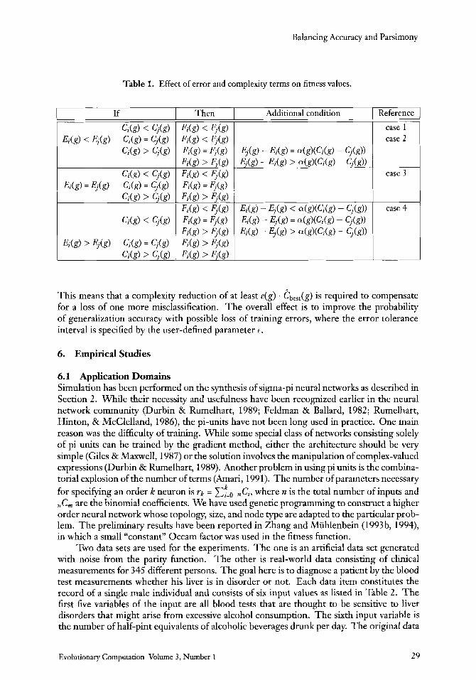
To see how the selection works based on this fitness evaluation scheme, we consider the fitness difference of two individuals, i andj, for Eb,,,(g - 1) I E :

IFt(g) - F,(g)l = IEiW - Ej(g) + a(g>(Ci(g> - C,<g>>I * (56)

There are nine possible relationships between Fi(g) and $(g) as listed in the first column of Table 1. Because the objective is to minimize the fitness, we are interested in the cases in which Fi(g) is less than F,(g) and i is selected againstj. There are four of them as marked in the rightmost column of the table.

Case 1: Ei(g) < Ej(g) and Ci(g) < q ( g ) . This is a trivial case; if i has less error and lower complexity thanj, Fi(g) will be less than F,(g).

Case 2 : Ei(g) < Ej(g) and Ci(g) = q ( g ) . When both have the same complexity, i must have less error thanj in order for Fi(g) to be less than F,(g).

Case 3 : &(g) = Ej(g) and Ci(g) < Cj(g). When the errors of both individuals are the same, the complexity of i must be lower than that ofj.

0 Case 4: Ei(g) > $(g) and Ci(g) < C,(g). Although individual i has larger error thanj, the fitness of i can be smaller than that o f j if the complexity of i is much smaller than the complexity ofj.

The last case is worthy ofmore discussion. Here we haveEi(g) > Ej(g) and Ci(g) < C,(g) and want to study the condition for F;(g) < F,(g), which can be rewritten as

4g)<C,(g) - Ci(g)> > W g ) - E,(g)- (5 7)

q(g> - C&) (5 8)

By substituting Equation ( 5 3 ) for Eb,,t(g - 1) 5 E into this inequality, we get

> N2 ' Ebest(g - 1) ' Cbest(g) ' (Ei(g> - Ej(g))- Let Ebest(g - 1) = e(g)/N, where N is the number of training examples and e(g) is the number of mismatched examples for the best individual in generation g. Then we have

q ( g ) - Ci<g) > e(g) ' ' t b e s t k ) . (Ei(g) - Ej(g))* (59)

q < g ) - Ci(g) > e(g) ' ebest(g). (60)

Ln the case of E;(g) - $(g) = 1/N, that is, the ith program correctly classifies one more data than thejth, the complexity reduction must satisfy the relation



Table 1. Effect of error and complexity terms on fitness values.

This means that a complexity reduction of at least e(g) . tbest(g) is required to compensate for a loss of one more misclassification. The overall effect is to improve the probability of generalization accuracy with possible loss of training errors, where the error tolerance interval is specified by the user-defined parameter E.

6. Empirical Studies

6.1 Application Domains Simulation has been performed on the synthesis of sigma-pi neural networks as described in Section 2. While their necessity and usefulness have been recognized earlier in the neural network community (Durbin & Rumelhart, 1989; Feldman & Ballard, 1982; Rumelhart, Hinton, & McClelland, 1986), the pi-units have not been long used in practice. One main reason was the difficulty of training. While some special class of networks consisting solely of pi units can be trained by the gradient method, either the architecture should be very simple (Giles & Maxwell, 1987) or the solution involves the manipulation of complex-valued expressions (Durbin & Rumelhart, 1989). Another problem in using pi units is the combina- torial explosion of the number of terms (Amari, 1991). The number of parameters necessary for specifymg an order k neuron is rk = nC;, where n is the total number of inputs and .C, are the binomial coefficients. We have used genetic programming to construct a higher order neural network whose topology, size, and node type are adapted to the particular problem. The preliminary results have been reported in Zhang and Miihlenbein (1993b, 1994), in which a small “constant” Occam factor was used in the fitness function.

Two data sets are used for the experiments. The one is an artificial data set generated with noise from the parity function. The other is real-world data consisting of clinical measurements for 345 different persons. The goal here is to diagnose a patient by the blood test measurements whether his liver is in disorder or not. Each data item constitutes the record of a single male individual and consists of six input values as listed in Table 2. The first five variables of the input are all blood tests that are thought to be sensitive to liver disorders that might arise from excessive alcohol consumption. The sixth input variable is the number of half-pint equivalents of alcoholic beverages drunk per day. The original data

k



Table 2. Attribute information in blood tests for liver diagnosis.

Attribute

x4

x5 x6

Name mcv alkphos smt sgot gammagt drinks

Description mean corpuscular volume alkaline phosphotase alamine aminotransferase aspartate aminotransferase gamma-glutamyl transpeptidase alcoholic beverages drunk per day

values (Murphy & Aha, 1994) were normalized into the interval [ - 1,1] before being used to train the networks.

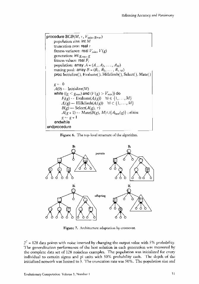
6.2 Method The algorithm is summarized in Figure 6. At the start, the initial population A(0) of M networks is created at random. The random initialization includes the type and receptive field of units, the depth of the network, and the weight values. For the gth population, the fitness of each member network, Fj(g), is evaluated by the adaptive fitness function in Equation (54).

Each member of the population undergoes a hill-climbing search in which a fixed number of local search steps are performed while the structure is fixed. Each local search step consists of a random modification of the weight values, followed by its fitness evaluation, and the acceptance or rejection of new configuration. The new configuration is accepted as the current one if the new individual is fitter than the current one. Otherwise the previous one is used as the current individual. Hill climbing turned out to be useful from our previous observation that once the average size of individuals grows, it gets more difficult to find a smaller solution, although the solutions exist in the smaller subspace.

The best 7% of the hill-climbed population of generationg are selected into the mating pool D(g), where 7 E (0,1] is the truncation threshold (Miihlenbein & Schlierkamp-Voosen, 1993). The (g i 1)th generation of size M is produced by applying crossover and mutation operators to the parent networks in the mating pool B(g). New populations are generated until the variance of fitness values falls below the specified limit V- or the generation number reaches gm,.

The crossover operator selects two parents, Bi and 4 at random, and exchanges their subtrees to create two offspring B: and Bj (see Figure 7). In this way, the size, depth, and receptive field shape of the network architecture are adapted. In Figure 7, for example, the number of units of parent Bi has increased by replacing one of its pi-subtrees with the sigma- sigma-pi-subtree of parent 4. The weights are adapted by repeatedly applying a mutation operator to each individual. The mutation operator also changes the index for the input units and the neuron type. For instance, a sigma unit is mutated to a pi unit and vice versa. This flexibility gives the chance of evolving conventional neural network architectures as well as networks consisting of any combinations of sigma and pi units.

6.3 Simulation Results The performance of the method for solving the parity problem of seven inputs is shown in Figure 8. The training set consists of 64 examples that were chosen randomly from



irocedure BGP(M, 7 , V,in, g,,,) population size: int M truncation rate: real 7

fitness variance: real V,,,in, V(g) generation: int g,,,, g fimess values: real F, population: array A = (Al, A 2 , . . . , AM) mating pool: array B = (B , , B2, . . . , BT.M) proc Initialize( ), Evaluate( ), Hillclimb( ), Select( ), Mate( )

Figure 6. The top-level structure of the algorithm.

Bi Bj

I

Figure 7. Architecture adaptation by crossover.

Z 7 = 128 data points with noise inserted by changing the output value with 5 % probability. The generalization performance of the best solution in each generation was measured by the complete data set of 128 noiseless examples. The population was initialized for every individual to contain sigma and pi units with 50% probability each. The depth of the initialized network was limited to 3 . The truncation rate was 50%. The population size and



200 -

150- Y ) . x . 0 .

$ 100:

50 -

0

0.5

-

.. . .. . .. ---- _____----_____ 7-- , - . I - - . - ' ' . - ' ~ l - I ,.,""-r---

---- ....... :.. . . . . ., , .. . . . .

.............. - - - - - ...--------. ___-_- -

training error . . . . . . . . . .. . generalization error .......... ~~. ... .

. -. . .. ,

0.0 rrrrT I . . . l . . . .rp ' ' ~ " " '

0 5 10 15 20 25 30 35 40 45 50

generation

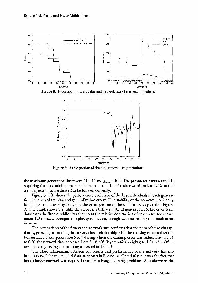
Figure 8. Evolution of fitness value and network size of the best individuals.

0

I

0.5 4.. . . . , . . . . . , . . . . . , . . . . . , . . . . . , . . . . . , . . . . . , . . . . . , . . . . . , . . . .A 0 5 10 15 20 25 30 35 40 45 50

generation

Figure 9. Error portion of the total fitness over generations.

the maximum generation limit were M = 40 and g,,, = 100. The parameter E was set to 0.1, requiring that the training error should be at most 0.1 or, in other words, at least 90% of the training examples are desired to be learned correctly.

Figure 8 (left) shows the performance evolution of the best individuals in each generation, in terms of training and generalization errors. The stability of the accuracy-parsimony balancing can be seen by analyzing the error portion of the total fitness depicted in Figure 9. The graph shows that until the error falls below E = 0.1 at generation 26, the error term dominates the fitness, while after that point the relative domination of error term goes down under 1.0 to make stronger complexity reduction, though without riskmg too much error increase.

The comparison of the fitness and network size confirms that the network size change, that is, growing or pruning, has a very close relationship with the training error reduction. For instance, from generation 6 to 7 during which the training error was reduced from 0.3 1 to 0.28, the network size increased from 3-18-105 (layers-units-weights) to 4-2 1-126. Other examples of growing and pruning are listed in Table 3.

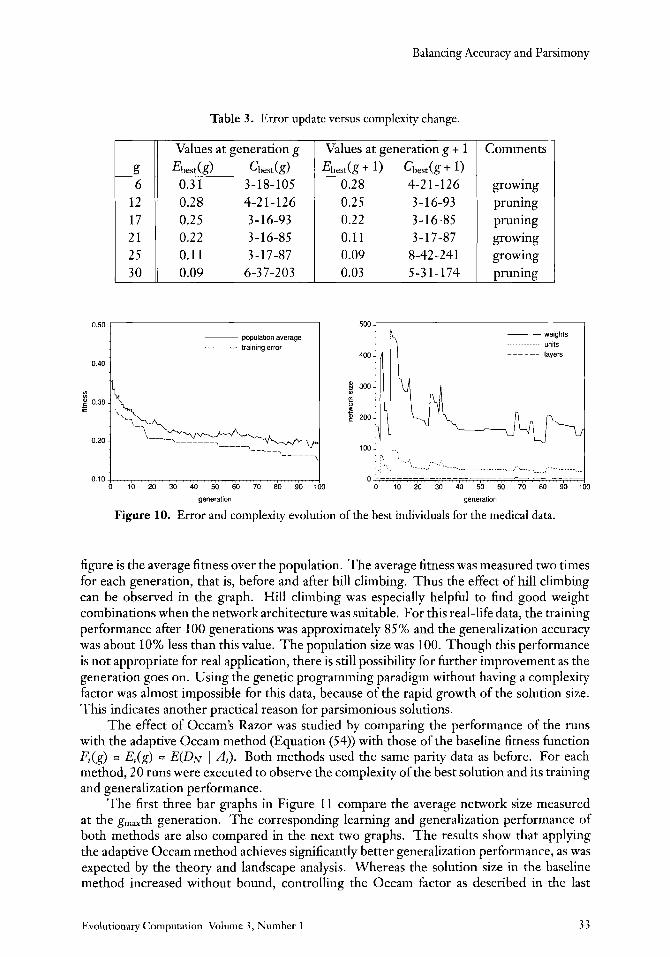
The close relationship between complexity and performance of the network has also been observed for the medical data, as shown in Figure 10. One difference was the fact that here a larger network was required than for solving the parity problem. Also shown in the

3 2 Evolutionary Computation Volume 3, Number 1


E b e s d g ) Cbedg) 0.3 1 3- 18- 105 0.28 4-2 1 - 126 0.2 5 3-16-93 0.22 3 - 16-85 0.11 3-17-87 0.09 6-37-203

g 6

12 17 21 25 30

, Ehe& + l ) c b e s t ( g +

0.28 4-2 1 - 12 6 growing 0.25 3- 16-93 pruning 0.22 3-16-85 pruning 0.1 1 3-17-87 growing 0.09 8-42-241 growing 0.03 5-31-174 pruning

Table 3. Error update versus complexity change.

0.50 ~

0.40 .

Values at generation g I Values at generation g + 1 I Comments

population average training error

layers _ _ _ _ - _ .... ~~ ~~...

-_--_-_ --.-- 0.10, , ,..,..,.....I..---T-. , . . . , . . . , . , . . . ~

figure is the average fitness over the population. The average fitness was measured two times for each generation, that is, before and after hill climbing. Thus the effect of hill climbing can be observed in the graph. Hill climbing was especially helpful to find good weight combinations when the network architecture was suitable. For this real-life data, the training performance after 100 generations was approximately 85 % and the generalization accuracy was about 10% less than this value. The population size was 100. Though this performance is not appropriate for real application, there is still possibility for further improvement as the generation goes on. Using the genetic programming paradigm without having a complexity factor was almost impossible for this data, because of the rapid growth of the solution size. This indicates another practical reason for parsimonious solutions.

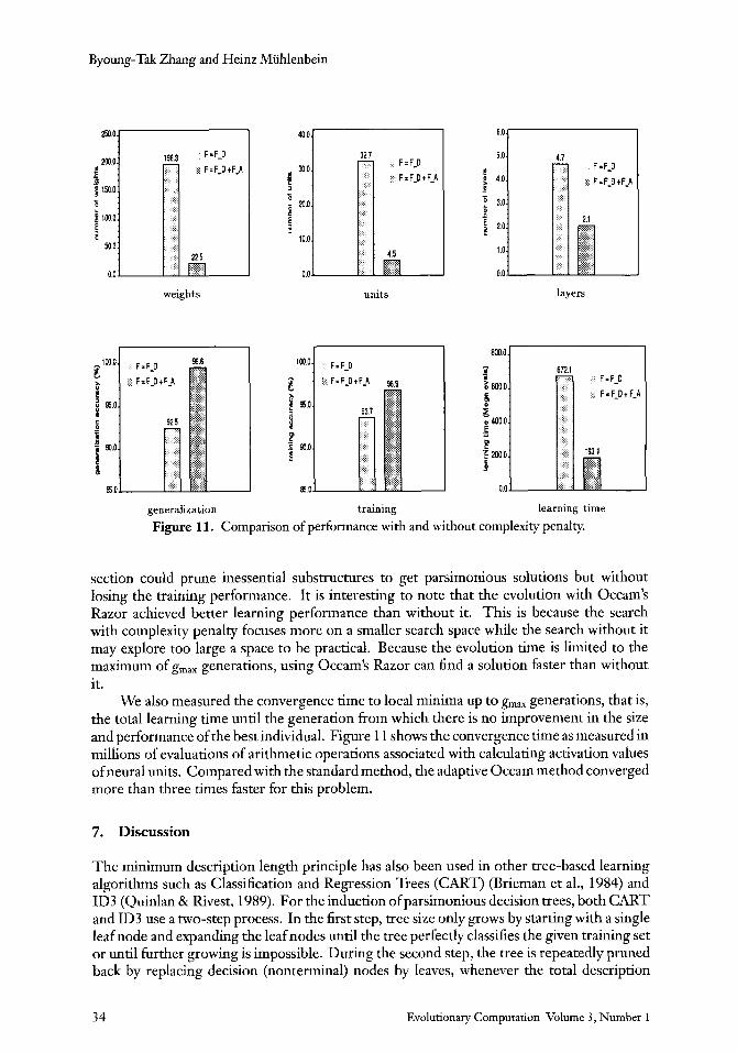
The effect of Occam’s Razor was studied by comparing the performance of the runs with the adaptive Occam method (Equation (54)) with those of the baseline fitness function Fi(g) = E,(g) = E(DN I Ai). Both methods used the same parity data as before. For each method, 20 runs were executed to observe the complexity of the best solution and its training and generalization performance.

The first three bar graphs in Figure 11 compare the average network size measured at the g,,,th generation. The corresponding learning and generalization performance of both methods are also compared in the next two graphs. The results show that applying the adaptive Occam method achieves significantly better generalization performance, as was expected by the theory and landscape analysis. Whereas the solution size in the baseline method increased without bound, controlling the Occam factor as described in the last

Evolutionary Computation Volume 3 , Number 1 3 3


250 0

2w 0 r f 1600

6 1wo

0

-

50 0

00

weights

generalization

units

training

5 0

E 40

3 0 3

s 5 2 0

1 0

00

layers

learning time

Figure 11. Comparison of performance with and without complexity penalty.

section could prune inessential substructures to get parsimonious solutions but without losing the training performance. It is interesting to note that the evolution with Occam's Razor achieved better learning performance than without it. This is because the search with complexity penalty focuses more on a smaller search space while the search without it may explore too large a space to be practical. Because the evolution time is limited to the maximum of g,, generations, using Occam's Razor can find a solution faster than without it.

We also measured the convergence time to local minima up to g,,, generations, that is, the total learning time until the generation from which there is no improvement in the size and performance of the best individual. Figure 1 1 shows the convergence time as measured in millions of evaluations of arithme tic operations associated with calculating activation values of neural units. Compared with the standard method, the adaptive Occam method converged more than three times faster for this problem.

7. Discussion

The minimum description length principle has also been used in other tree-based learning algorithms such as Classification and Regression Trees (CART) (Brieman et al., 1984) and ID3 (Quinlan & Rivest, 1989). For the induction of parsimonious decision trees, both CART and ID3 use a two-step process. In the first step, tree size only grows by starting with a single leaf node and expanding the leaf nodes until the tree perfectly classifies the given training set or until further growing is impossible. During the second step, the tree is repeatedly pruned back by replacing decision (nonterminal) nodes by leaves, whenever the total description



length is reduced. The total description length is defined as the sum of the tree coding length and the error coding length in bits. Note that in this two-step induction, the tree complexity is considered only in the pruning phase. This is equivalent to a strategy of first reducing the error and then reducing the complexity.

One fundamental difference between the genetic programming approach (including our method) and conventional tree-induction methods is that a population of trees is used instead of a single tree. In the genetic programming approach, pruning and growing are interleaved during the learning process. This is primarily done by the crossover operator, which generates new trees that can be larger or smaller than their parents.

Iba et al. have used the MDL principle in genetic programming to evolve GMDH networks (Ivakhnenko, 1971) and decision trees (Iba, Kurita, de Garis, & Sato, 1993; Iba, de Garis, & Sato, 1994). As in ID3, the code length (CL) is defined as the total sum of description lengths:

cLi(g) = E(D I A;) + C(A$), (61)

where C(A$) is the description length for the tree A$ and E(D 1 A$) is the coding length for the classification error of the tree for the training set D. The description lengths are defined with respect to a specific encoding scheme chosen by the author. Due to the unknown range3 of the total coding length, a scaling window of size Wsize is used to determine a normalization factor, CL,,,(g). CL,,x(g) is defined as the largest code length during the last Wsize generations. The fitness value of the tree is then defined as

Notice that the fitness is defined here as simply the sum of error and complexity costs, followed by a normalization of the total costs. Therefore, the complexity value C(Ak) is as important as the error value E(D I A?) in determining the total fitness value of an individual. This works perfectly when the coding scheme exactly reflects the true probability distribution of the environment. One possible drawback in this implementation of the MDL principle in genetic programming is the lack of flexibility in balancing accuracy with parsimony in unknown environments. That is, there is a risk that the network size may be penalized too much, resulting in premature convergence in spite of other diversity-increasing measures, such as a large crossover rate. In fact, the authors remark that this kind of MDL approach should be used carefully when evolving general programs with genetic programming (Iba et al., 1994). Note also that this strategy is far from the two-step approach of ID3, taken to ensure parsimonious solutions without losing good performance.

Premature convergence in the direct MDL approach can be avoided by introducing a small Occam factor a(,):

where Ei(g) and Ci(g) are the error and complexityvalues normalized separately, and a(g) is a constant expressed as a function of the training set size (Zhang & Miihlenbein, 1993a; Zhang & Miihlenbein, 199313). In this MDL approach, the complexity cost influences the selection process only when the candidates for selection have comparable performance. That is, a tree wins the selection only if its error is smaller than that of its competitors, or its error is the same as its competitors but its size is smaller. Note that this is an evolutionary equivalent of the strategy of first reducing the error and then reducing the complexity. Experimental

3 The range of the coding length vanes from --oc to cy. due to the use of logarithms in calculating the length in bits.

Evolutionary Computation Volume 3, Number 1 3 5


evidence shows this method is robust and effective for a wide class of tasks. However, this balancing mechanism is very conservative and can still be speeded up by making the control of the Occam factor more flexible.

The adaptive Occam method described in this article improves the fixed Occam approach by changing the ratio of error to complexity in the course of the run. In early stages of learning, a strong increase in tree complexity is allowed by keeping the Occam factor small, which usually results in fast error reduction. The small Occam factor also results in robust convergence to the desired training accuracy, because premature convergence is avoided due to increased diversity. In later stages, that is, after the desired level of training performance is achieved, the adaptive Occam approach enforces a strong complexity penalty, which encourages parsimony. Overall, this has the effect of increasing generalization performance without getting stuck in local minima due to premature convergence. The control of the phase transition is not difficult because it is defined by the desired training accuracy that the user requires. Though other MDL-based tree induction methods also reward parsimony, the adaptive Occam approach is different in that it dynamically balances error and complexity

While proposed in a different context, the adaptive fitness function presented in this article has some similarity in spirit to cornpetitiveJihzessJicnctions (Angeline & Pollack, 1993). Standard fitness functions return the same fitness for an individual regardless of what other members are present in the population, demanding an accurate and consistent fitness measure throughout the evolutionary process. While the global accuracy can be easily computed when evolving solutions for many simple problems, it is often impractical for problems with greater complexity. In contrast, competitive fitness functions evaluate the fitness values depending on the constituents of the population. Angeline argues that competitive fitness functions provide a more robust training environment than independent fitness functions.

A final comment is in order on the applicability of this approach to the more general classes of programs that can be developed by genetic programming. The general method of balancing accuracy and parsimony can be used for the genetic induction of other classes of tree-structured programs as well. This is because the error and complexity values are normalized separately and the same adaptive balancing mechanism can be used for different definitions of error and complexity.

costs.

8. Conclusion

We have investigated the theoretical relationship between the complexity of a solution and its generalization ability in genetic programming. An analysis of the fitness landscape was made in the context of inferring sigma-pi neural networks from data. The comparison of learning and generalization performance as a function of network size suggests the effectiveness of minimal-complexity approaches.

We presented an adaptive method that obtains parsimonious solutions while guarantee- ing the specified minimal training accuracy with a high probability. The method implements a kind of dynamic search where the focus of attention depends on the structure of the current and past fitness landscapes, that is, the distribution of error and complexity of the individuals in the recent populations. Whereas pruning is always encouraged by the nonzero Occam factor, the adaptive fitness function simultaneously promotes growing if it is necessary for significant error reduction.

Though our experiments were performed in the context of neural network synthesis, the underlying principle of balancing accuracy with parsimony applies to all genetic program-



ming applications in which the structural complexity, as well as the structures themselves, should be optimized on the basis of noisy or incomplete data.

Acknowledgment This research was supported in part by the Real-World Computing Program under the project SIFOGA. We thank Jiirgen Bendisch, Gerd PaaB, Mark Rmg, and Dirk Schlierkamp- Voosen for helpful discussions.

References Amari, S.-I. (1991). Dualistic geometry of the manifold of higher-order neurons. Neural Networks, 4,

4 4 3 4 5 1.

Angeline, P. J., & Pollack, J. B. (1993). Competitive environments evolve better solutions for complex tasks. In S. Forrest (Ed.), Proceedings of the Fijih International Conference on GeneticAlgorithms (ICGA- 93) (pp. 264-270). San Mateo, CA: Morgan Kaufmann.

Back, T., & Schwefel, H.-P. (1993). An overview of evolutionary algorithms for parameter optimization. Evolutiona7y Computation, 1(1), 1-23.

Blumer, A,, Ehrenfeucht, A., Haussler, D., & Warmuth, M. K. (1987). Occam’s Razor. Information Processing Letters, 24, 377-380.

Breiman, L., Friedman, J. H., Olshen, R. A., & Stone, C. J. (1984). Classzjication and regression trees. Belmont, CA: Wadsworth International Group.

Carbonell, J. G. (1990). Introduction: Paradigms for machine learning. In J. G. Carbonell (Ed.), Machine learning: Paradigms and methods (pp. 1-9). Cambridge, MA: MIT Press.

Durbin, R., & Rumelhart, D. E. (1989). Product units: A computationally powerful and biologically plausible extension to backpropagation networks. Neural Computation, 1, 133-142.

Feldman, J. A., & Ballard, D. H. (1982). Connectionist models and their properties. Cognitive Science, 6,205-254.

Fogel, D. B. (1991). An information criterion for optimal neural network selection. IEEE Transactions on Neural Networks, 2(5), 490-497.

Geman, S., Bienenstock, E., & Doursat, R. (1992). Neural networks and the biaslvariance dilemma. Neural Computation, 4 , 1-58.

Giles, C. L., & Maxwell, T. (1987). Learning, invariance, and generalization in high-order neural networks. Applied Optics, 26(23), 4972-4978.

Goldberg, D. E. (1989). Genetic algorithms in search, optimization & machine learning. Reading, MA: Addison-Wesley.

Iba, H., de Garis, H., & Sato, T. (1994). Genetic programming using a minimum description length principle. In K. E. Kinnear (Ed.), Advances in genetic programming (pp. 265-284). Cambridge, MA: MIT Press.

Iba, H., Kurita, T., de Garis, H., & Sato, T. (1993). System identification using structured genetic algorithms. In S. Forrest (Ed.), Proceedings of the FiBh International Conference on Genetic Algorithms (ZCGA-93) (pp. 279-286). San Mateo, CA: Morgan Kaufmann.

Ivakhnenko, A. G. (1971). Polynomial theory of complex systems. IEEE Transactions on Systems, Man, and Cybernetics, 1(4), 364-378.

Kinnear, K. E. (1993). Generality and difficulty in genetic programming: Evolving a sort. In S. Forrest (Ed.), Proceedings of the Fi$h International Conference on Genetic Algorithms (ICGA-93) (pp. 287-294). San Mateo, CA: Morgan Kaufmann.

Kinnear, K. E. (Ed.). (1994a). Advances in geneticprogvamming. Cambridge, MA: MIT Press.

Evolutionary Computation Volume 3, Number I 37


Kinnear, K. E. (1994b). Fitness landscapes and difficulty in genetic programming. In Proceedings of ZEEE International Confrence on Evolutionary Computation (ICEC-94), World Congress on Computational Intelligence (pp. 142-147). New York: IEEE Computer Society Press.

Koza, J. R. (1992a). Genetic programming: On the programming of computers by means of natural selection. Cambridge, MA. MIT Press.

Koza, J. R. (1992b). Hierarchical automatic function definition in genetic programming. In D. Whitley (Ed.), Foundations of Genetic Algorithms (FOGA-92) (pp. 24-29). San Mateo, CA: Morgan Kaufmann.

Koza, J. R. (1993). Simultaneous discovery of reusable detectors and subroutines using genetic programming. In S. Forrest (Ed.), Proceedings of the Fij?h International Coizference on Genetic Algorithms (pp. 29.5-302). San Mateo, CA: Morgan Kaufmann.

Koza, J. R. (1994). Genetic programming ZZ: Automatic discovery of reusable programs. Cambridge, MA: MIT Press.

Manderick, B., de Weger, M., & Spiessens, P. (1991). The genetic algorithm and the structure of the fitness landscape. In R. K. Belew and L. B. Booker (Eds.), Proceedings of the Fourth Znternational Conference on Genetic Algorithms (pp. 143-1 S O ) . San Mateo, CA: Morgan Kaufmann.

Miihlenbein, H., & Schlierkamp-Voosen, D. (1993). Predictive models for the breeder genetic algorithm I: Continuous parameter optimization. Evolutionary Computation, I (I), 2 S49 .

Murphy, P. M., & Aha, D. W. (1994). UCZrepository ofmachine learning databases. [Electronic database] Department of Information and Computer Science, University of California, Irvine.

Quinlan, J. R., & Rivest, R. L. (1989). Inferring decision trees using the minimum description length principle. Znfrmation and Computation, 80,227-248.

Rissanen, J. (1984). Universal coding, information, prediction, and estimation. ZEEE Transations on Infmation Theory, ?0(4), 629-636.

Rissanen, J. (1986). Stochastic complexity and modeling. The Annals of Statistics, 14, 1080-1 100.

Rumelhart, D. E., Hinton, G. E., & McClelland, J. L. (1986). A general framework for parallel distributed processing. In D. E. Rumelhart and J. L. McClelland (Eds.), Parallel distributedprocessing, Vol. I (pp. 45-76). Cambridge, MA: MIT Press.

Samuel, A. L. (1 963). Some studies in machine learning using the game of checkers. In E. Feigenbaum and J. Feldman (Eds.), Computers and thought (pp. 71-105). New York: McGraw-Hill.

Tackett, W. A. (1993). Genetic programming for feature discovery and image discrimination. In S. Forrest (Ed.), Proceedings of the F$h International Conference on Genetic Algorithms (ICGA-93) (pp. 303-309). San Mateo, CA: Morgan Kaufmann.

Winston, P. (1975). Learning structural descriptions from examples. In Patrick H. Winston (Ed.), The psychology of computer vision (pp. 157-209). New York: McGraw-Hill.

Zhang, B.-T. (1994). Effects of Occam’s razor in evolving sigma-pi neural networks. In Y. Davidor, H.-P. Schwefel, and R. Manner (Eds.), Lecture notes in computer science 866: Parallel problem solving

f;om nature (pp. 462471). London: Springer-Verlag.

Zhang, B.-T., & Miihlenbein, H. (1993a). Evolving optimal neural networks using genetic algorithms with Occam’s razor. Complex Systems, 7(3), 199-220.

Zhang, B.-T., & Miihlenbein, H. (1993 b). Genetic programming of minimal neural nets using Occam’s razor. In S. Forrest (Ed.), Proceedings of the Fifth International Conference on Genetic Algorithms (ICGA- 93) (pp. 342-349). San Mateo, CA: Morgan Kaufmann.

Zhang, B.-T, & Muhlenbein, H. (1994). Synthesis of sigma-pi neural networks by the breeder genetic programming. In Proceedings of ZEEE International Conference on Evolutionary Computation QCEC- 94), World Congress on Computational Intelligence (pp. 3 18-32 3). New York: IEEE Computer Society Press.


This article has been cited by:

1. Riccardo Poli, Leonardo Vanneschi, William B. Langdon, Nicholas Freitag McPhee. 2010. Theoreticalresults in genetic programming: the next ten years?. Genetic Programming and Evolvable Machines11:3-4, 285-320. [CrossRef]

2. David Kinzett, Mark Johnston, Mengjie Zhang. 2009. Numerical simplification for bloat control andanalysis of building blocks in genetic programming. Evolutionary Intelligence 2:4, 151-168. [CrossRef]

3. Peyman Kouchakpour, Anthony Zaknich, Thomas Bräunl. 2009. A survey and taxonomy ofperformance improvement of canonical genetic programming. Knowledge and Information Systems 21:1,1-39. [CrossRef]

4. Sara Silva, Ernesto Costa. 2009. Dynamic limits for bloat control in genetic programming and areview of past and current bloat theories. Genetic Programming and Evolvable Machines 10:2, 141-179.[CrossRef]

5. Ekaterina J. Vladislavleva, Guido F. Smits, Dick den Hertog. 2009. Order of Nonlinearity as aComplexity Measure for Models Generated by Symbolic Regression via Pareto Genetic Programming.IEEE Transactions on Evolutionary Computation 13:2, 333-349. [CrossRef]

6. Bart Wyns, Luc Boullart. 2009. Efficient tree traversal to reduce code growth in tree-based geneticprogramming. Journal of Heuristics 15:1, 77-104. [CrossRef]

7. Mengjie Zhang, Phillip Wong. 2008. Genetic programming for medical classification: a programsimplification approach. Genetic Programming and Evolvable Machines 9:3, 229-255. [CrossRef]

8. Xiao-Bing Hu, Ezequiel Di Paolo, Shu-Fan Wu. 2008. A comprehensive fuzz-rule-based self-adaptivegenetic algorithm. International Journal of Intelligent Computing and Cybernetics 1:1, 94-109.[CrossRef]

9. Andrew Kusiak, Filippo A. Salustri. 2007. Computational Intelligence in Product Design Engineering:Review and Trends. IEEE Transactions on Systems, Man and Cybernetics, Part C (Applications andReviews) 37:5, 766-778. [CrossRef]

10. Sean Luke, Liviu Panait. 2006. A Comparison of Bloat Control Methods for Genetic ProgrammingAComparison of Bloat Control Methods for Genetic Programming. Evolutionary Computation 14:3,309-344. [Abstract] [PDF] [PDF Plus]

11. Chi Zhou, Weimin Xiao, T.M. Tirpak, P.C. Nelson. 2003. Evolving accurate and compactclassification rules with gene expression programming. IEEE Transactions on EvolutionaryComputation 7:6, 519-531. [CrossRef]

12. Riccardo Poli , Nicholas Freitag McPhee . 2003. General Schema Theory for Genetic Programmingwith Subtree-Swapping Crossover: Part IIGeneral Schema Theory for Genetic Programming withSubtree-Swapping Crossover: Part II. Evolutionary Computation 11:2, 169-206. [Abstract] [PDF][PDF Plus]

13. Sean Luke . 2003. Modification Point Depth and Genome Growth in GeneticProgrammingModification Point Depth and Genome Growth in Genetic Programming. EvolutionaryComputation 11:1, 67-106. [Abstract] [PDF] [PDF Plus]

14. N.Y. Nikolaev, H. Iba. 2001. Regularization approach to inductive genetic programming. IEEETransactions on Evolutionary Computation 5:4, 359-375. [CrossRef]

15. Ricardo S. Zebulum , Marley Vellasco , Marco Aurélio Pacheco . 2000. Variable Length Representationin Evolutionary ElectronicsVariable Length Representation in Evolutionary Electronics. EvolutionaryComputation 8:1, 93-120. [Abstract] [PDF] [PDF Plus]

16. S. Luke. 2000. Two fast tree-creation algorithms for genetic programming. IEEE Transactions onEvolutionary Computation 4:3, 274-283. [CrossRef]

http://dx.doi.org/10.1007/s10710-010-9110-5

http://dx.doi.org/10.1007/s12065-009-0029-9

http://dx.doi.org/10.1007/s10115-008-0184-9

http://dx.doi.org/10.1007/s10710-008-9075-9

http://dx.doi.org/10.1109/TEVC.2008.926486

http://dx.doi.org/10.1007/s10732-007-9060-0

http://dx.doi.org/10.1007/s10710-008-9059-9

http://dx.doi.org/10.1108/17563780810857149

http://dx.doi.org/10.1109/TSMCC.2007.900669

http://dx.doi.org/10.1162/evco.2006.14.3.309

http://www.mitpressjournals.org/doi/pdf/10.1162/evco.2006.14.3.309

http://www.mitpressjournals.org/doi/pdfplus/10.1162/evco.2006.14.3.309

http://dx.doi.org/10.1109/TEVC.2003.819261

http://dx.doi.org/10.1162/106365603766646825

http://www.mitpressjournals.org/doi/pdf/10.1162/106365603766646825

http://www.mitpressjournals.org/doi/pdfplus/10.1162/106365603766646825

http://dx.doi.org/10.1162/106365603321829014



http://dx.doi.org/10.1109/4235.942530

http://dx.doi.org/10.1162/106365600568112



http://dx.doi.org/10.1109/4235.873237

17. A.E. Eiben, R. Hinterding, Z. Michalewicz. 1999. Parameter control in evolutionary algorithms. IEEETransactions on Evolutionary Computation 3:2, 124-141. [CrossRef]

18. Donald S. Burke, Kenneth A. De Jong, John J. Grefenstette, Connie Loggia Ramsey, Annie S.Wu. 1998. Putting More Genetics into Genetic AlgorithmsPutting More Genetics into GeneticAlgorithms. Evolutionary Computation 6:4, 387-410. [Abstract] [PDF] [PDF Plus]

19. Terence Soule, James A. Foster. 1998. Effects of Code Growth and Parsimony Pressure on Populationsin Genetic ProgrammingEffects of Code Growth and Parsimony Pressure on Populations in GeneticProgramming. Evolutionary Computation 6:4, 293-309. [Abstract] [PDF] [PDF Plus]

http://dx.doi.org/10.1109/4235.771166







Documents

Balancing Accuracy and Parsimony in Genetic Programming 1995... · Balancing Accuracy and Parsimony in Genetic Programming Byoung-Tak Zhang Heinz Miihlenbein German National Research