Balance Sheets, Transaction Matrices and the Monetary … Lavoie 2007 chap02 … · · 2010-06-03Balance Sheets, Transaction Matrices and the Monetary Circuit ... consumption, accumulation

LAVOIE: “CHAP02” — 2006/9/11 — 10:01 — PAGE 23 — #1

2Balance Sheets, Transaction Matricesand the Monetary Circuit

2.1 Coherent stock-flow accounting

Contemporary mainstream macroeconomics, as it can be found inintermediate textbooks, is essentially based on the system of nationalaccounts that was put in place by the United Nations in 1953 – the so-calledStone accounts. At that time, some macroeconomists were already search-ing for some alternative accounting foundations for macroeconomics. In theUnited States, Morris A. Copeland (1949), an institutionalist in the quantita-tive Mitchell tradition of the NBER, designed the first version of what becamethe flow-of-funds accounts now provided by the Federal Reserve since 1952 –the Z.1 accounts. Copeland wanted to have a framework that would allowhim to answer simple but important questions such as: ‘When total purchasesof our national product increase, where does the money come from to financethem? When purchases of our national product decline, what becomes of themoney that is not spent?’ (Copeland 1949 (1996: 7)).

AQ: Pleasecheck.Copeland1996 is notlisted in thereferences

In a macroeconomic textbook that was well-known in France, Jean Denizet(1969) also complained about the fact that standard macroeconomic account-ing, designed upon Richard Stone’s social accounting, as eventually laidout in the 1953 United Nations System of National Accounts, left mon-etary and financial phenomena in the dark, in contrast to the approachthat was advocated from the very beginning by some accountants (amongwhich Denizet) in the Netherlands and in France. In the initial standardnational accounting – as was shown in its most elementary form with thehelp of Table 1.1 – little room was left for banks and financial intermedi-aries and the accounts were closed on the basis of the famous Keynesianequality, that saving must equal investment. This initial system of accountsis a system that presents ‘the sector surpluses that ultimately finance realinvestment’, but it does not present ‘any information about the flows infinancial assets and liabilities by which the saving moves through the finan-cial system into investment. These flows in effect have been consolidated out’(Dawson 1991 (1996: 315)). In standard national accounting, as represented

23

LAVOIE: “CHAP02” — 2006/9/11 — 10:01 — PAGE 24 — #2

24 Monetary Economics

by the National Income and Product Accounts (NIPA), there is no room todiscuss the questions that Copeland was keen to tackle, such as the changesin financial stocks of assets and of debts, and their relation with the transac-tions occurring in the current or the capital accounts of the various agentsof the economy. In addition, in the standard macroeconomics textbook,households and firms are often amalgamated within a single private sector,and hence, since financial assets or debts are netted out, it is rather diffi-cult to introduce discussions about such financial issues, except for publicdebt.

The lack of integration between the flows of the real economy and its finan-cial side greatly annoyed a few economists, such as Denizet and Copeland.For Denizet, J.M. Keynes’s major contribution was his questioning of theclassical dichotomy between the real and the monetary sides of the econ-omy. The post-Keynesian approach, which prolongs Keynes’s contributionon this, underlines the need for integration between financial and incomeaccounting, and thus constitutes a radical departure from the mainstream. 1

AQ: PleasecheckCopeland(1973) is notlisted inreferences.

Denizet found paradoxical that standard national accounting, as was initiallydeveloped by Richard Stone, reproduced the very dichotomy that Keynes hadhimself attempted to destroy. This was surprising because Stone was a goodfriend of Keynes, having provided him with the national accounts data thatKeynes needed to make his forecasts and recommendations to the BritishTreasury during the Second World War, but of course it reflected the initialdifficulties in gathering enough good financial data, as Stone himself latergot involved in setting up a proper framework for financial flows and balancesheet data (Stone 1966).2

By 1968 a new System of National Accounts (SNA) was published by thenational accountants of the UN. This new system provided a theoreticalscheme that stressed the integration of the national income accounts withfinancial transactions, capital stocks and balance sheet (as well as input-output accounts), and hence answered the concerns of economists such asCopeland and Denizet. The new accounting system was cast in the formof a matrix, which started with opening assets, adding or subtracting pro-duction, consumption, accumulation and taking into account reevaluations,to obtain, at the bottom of the matrix, closing assets. This new integratedaccounting system has been confirmed with the revised 1993 SNA.

1 Such an integration of financial transactions with real transactions, within anappropriate set of sectors, was also advocated by Gurley and Shaw (1960: ch. 2) intheir well-known book, as it was by a number of other authors, inspired by the workof Copeland, Alan Roe (1973) for instance, whose article was appropriately titled ‘thecase for flow of funds and national balance sheet accounts’.

2 Various important surveys of flow-of-funds analysis and a stock-flow-consistentapproach to macroeconomics can be found, among others in Bain (1973), Davis (1987),Patterson and Stephenson (1988), Dawson (1996).

LAVOIE: “CHAP02” — 2006/9/11 — 10:01 — PAGE 25 — #3

Balance Sheets, Transaction Matrices, Monetary Circuit 25

Several countries now have complete flow-of-funds accounts or financialflows accounts, as well as national balance sheet accounts, so that by combin-ing the flow-of-funds account and the national income and product account,and making a few adjustments, linked in particular to consumer durablegood, it is possible to devise a matrix that accomplishes such an integration,as has been demonstrated by Backus et al. (1980: 270–1). The problem nowis not so much the lack of appropriate data, as shown by Ruggles (1987), butrather the unwillingness of most mainstream macroeconomists to incorpo-rate these financial flows and capital stocks into their models, obsessed asthey are with the representative optimizing microeconomic agent. The con-struction of this integrated matrix, which we shall call the transactions flowmatrix, will be explained in a later section. But before we do so, let us examinea simpler financial matrix, one that is better known, the balance sheet matrixor the stock matrix.

2.2 Balance sheets or stock matrices

2.2.1 The balance sheet of households

Constructing the balance sheet matrix, which deals with asset and liabilitystocks, will help us understand the typical financial structure of a moderneconomy. It will also give clues as to the elements that ought to be found inthe transaction flow matrix.

Let us consider a simple closed economy. Open economies will not beexamined at this stage because, for the model to be fully coherent, one wouldneed to consider the whole world, that is, in the simplest open-economymodel, one would need to consider at least two countries.

Our simple closed economy contains the following four sectors: the house-hold sector, the production sector (made up of firms), the financial sector(essentially banks) and the government sector. The government sector canitself be split into two subsectors: the pure government sector and the cen-tral bank. The central bank is a small portion of the government sector, butbecause it plays such a decisive role with respect to monetary policy, andbecause its impact on monetary aggregates is usually identified on its own, itmay be preferable to identify it separately.

Before we describe the balance sheet matrix of all these sectors, that is,the sectoral balance sheet matrix, it may be enlightening, in the first stage,to look at the balance sheet of individual sectors. Let us deal for instancewith the balance sheet of households and that of production firms. First itshould be mentioned that this is an essential distinction. In many accounts ofmacroeconomics, households and firms are amalgamated into a single sector,that is, the private sector. But doing so, would lead to a loss in comprehendingthe functioning of the economy, for households and production firms takeentirely different decisions. In addition, their balance sheets show substantial

LAVOIE: “CHAP02” — 2006/9/11 — 10:01 — PAGE 26 — #4


differences of structure, which reflect the different roles that each sector plays.For the same reasons, it will be important to make a distinction betweenproduction firms (non-financial businesses) and financial firms (banks andthe so-called non-banking financial intermediaries).

We start with the balance sheet of households, since it is the most intu-itive as shown in Table 2.1. Households hold tangible assets (their tangiblecapital Kh). This tangible capital mainly consists of the dwellings that house-holds own – real estate – but it also includes consumer durable goods, such ascars, dishwashing machines or ovens. An individual may also consider thatthe jewellery (gold, diamonds) being kept at home or in a safe is part of tan-gible assets. But in financial flow accounts, jewellery is not included amongthe tangible assets. Households also hold several kinds of financial assets, forinstance bills Bh, money deposits Mh, cash Hh and a number e of equities,the market price of which is pe. Households also hold liabilities: they takeloans Lh to finance some of their purchases. For instance households wouldtake mortgages to purchase their house, and hence the remaining balance ofthe mortgage would appear as a liability.

The difference between the assets and the liabilities of households con-stitutes their net worth, that is, their net wealth NWh. The net worth ofhouseholds is a residual, which is usually positive and relatively substan-tial. This is because households usually spend much less than they receiveas income, and as a result they accumulate net financial assets and tangible(or real) assets. Note, however, that if equity prices (or housing prices) wereto fall below the value at which they were purchased with the help of loanstaken for pure speculative purposes – as would happen during a stock mar-ket crash that would have followed a stock market boom – the net worth ofhouseholds taken overall could become negative. This is because household

Table 2.1 Household balance sheet

Assets 64,000 Liabilities 64,400

Tangible capital Kh 25,500 Loans Lh 11,900Equities e · pe Net Worth NWh 52,100Bills BhMoney deposits Mh 5,900Cash Hh

Source: Z.1 statistics of the Federal Reserve, www.federalreserve.gov/releases/z1, Table B.100, ‘Balance sheet of households and nonprofitorganizations’, March 2006 release; units are billions of dollars.

LAVOIE: “CHAP02” — 2006/9/11 — 10:01 — PAGE 27 — #5


assets, in particular real estate and shares on the stock market, are valued attheir market value in the balance sheet accounts.3

In the case of American households, this is not likely to happen, basedon the figures presented in Table 2.1, which arise from the balance sheet ofhouseholds and nonprofit organizations, as assessed by the Z.1 statistics ofthe Federal Reserve for the last quarter of 2005. Loans represent less than 20%of net worth. Tangible assets – real estate and consumer durable goods – plusdeposits account for nearly 50% of total assets. The other financial assetsare not so easy to assign, since a substantial portion of these other assets,including equities and securities, are held indirectly, by pension funds, trustfunds and mutual funds.

In general net worth turns out to be positive. A general accounting principleis that balance sheets ought to balance, that is, the sums of all the items oneach side of the balance sheet ought to equal each other. It is obvious thatfor the balance sheet of households to balance, the item net worth must beadded to the liability side of the household balance sheet, since net worth ispositive and the asset value of households is larger than their liability value.

In the overall balance sheet matrix, all the elements on the asset side will beentered with a plus sign, since they constitute additions to the net worth ofthe sector. The elements of the liability side will be entered with a negativesign. This implies that net worth will be entered with a negative sign inthe balance sheet matrix, since it is to be found in the liability side. Theseconventions will insure that all the rows and all the columns of the balancesheet matrix sum to zero, thus providing consistency and coherence in ourstock accounting.

2.2.2 The balance sheet of production firms

It could be sufficient to deal with the household sector, since the balancesheets of all sectors respond to the same principles. The balance sheet of firms,however, suffers from one additional complication, which is worth lookingat. The complication arises from the existence of corporate equities. In somesense, the value of these shares is something which the firm owes to itself, butsince the owners consider the value of these shares to be part of their assets,it will have to enter the liability side of some other sector where we haveto be fully consistent. Equities pose a problem ‘because they are financialassets to whoever holds them, but they are not, legally, liabilities of theissuing corporation’ (Ritter 1963 (1996: 123)), in contrast to corporate paperor corporate bonds issued by the firm. This implies that interest payments

3 This is how it should be; but some statistical agencies still register real estate orstock market shares at their acquisition value.

LAVOIE: “CHAP02” — 2006/9/11 — 10:01 — PAGE 28 — #6


are a contractual obligation, whereas the payment of dividends is not – it isat the discretion of the board of directors.

However, in practice, as pointed out by Joan Robinson (1956: 247–8), thisdistinction becomes fuzzy since directors are reluctant to cut off dividends(because of the negative signal that it sends to the markets) and becausecreditors often will accept to forego interest payments temporarily to avoidthe bankruptcy of their debtor. As a result, as suggested by Ritter (1963 (1996:123)), ‘for most purposes the simplest way to handle this is to assume thatcorporate stocks and bonds are roughly the same thing, despite their legaldifferences and treat them both as liabilities of the corporation’.

This is precisely what we shall do. The current stock market value of thestock of equities which have been issued in the past shall be assessed as beingpart of the liabilities of the firms. By doing so, as will be clear in the nextsubsection, we make sure that a financial claim is equally valued whetherit appears among the assets of the households or whether it appears on theliability side of the balance sheet of firms. This will insure that the row ofequities in the overall sectoral balance sheet sums to zero, as all other rowsof the matrix. The balance sheet of production firms in our framework, willthus appear as shown in Table 2.2.

It must be noted that all the items on this balance sheet (except inventories)are evaluated at market prices. This distinction is important, because the itemson balance sheets of firms, or at least some items, are often evaluated athistorical cost, that is, evaluated at the price of acquisition of the assets andliabilities (the price paid at the time that the assets and liabilities were purchased).In the present book, balance sheets at market prices will be the rule. Thismeans that every tangible asset is evaluated at its replacement value, that is,the price that it would cost to produce this real asset now; and every financialasset is evaluated at its current value on the financial markets. For instance,a $100 bond issued by a corporation or a government may see its price risetemporarily to $120. With balance sheets evaluated at market prices, thebond will be entered as a $120 claim in the balance sheets of both the holder

Table 2.2 Balance sheet of production firms at market prices, with equities as a liability

Assets 2001 2005 Liabilities 2001 2005Total 17,500 22,725 Total 17,500 22,725

Tangible capital Kf 9,200 11,750 Loans Lf 9,100 10,125Financial assets Mf 8,300 11,975 Equities issued ef · pef 10,900 10,925

Net Worth NWf −2,500 +1675

Source: Z.1 statistics of the Federal Reserve, www.federalreserve.gov/releases/z1, Table B.102,‘Balance sheet of nonfarm nonfinancial corporate business’, March 2002 and 2006 releases, lastquarter data; units are billions of dollars.

LAVOIE: “CHAP02” — 2006/9/11 — 10:01 — PAGE 29 — #7


and the issuer of the bond, although the corporation or the government stilllook upon the bond as a $100 liability.

However, in the case of firms, the combination of equities treated as a debtof firms with market-price balance sheets yields counter-intuitive results. Thisis why it becomes important to study in detail the balance sheets of firms.Balance sheets computed at market prices and treating equities issued by firmsas a liability of the firm are the only ones that will be utilized in the bookbecause they are the only balance sheets which can be made coherent withinthe matrix approach which is advocated here.

In the example given by Table 2.2, firms have an array of tangible capital –fixed capital, real estate, equipment and software, and inventories, which,evaluated at production prices or current replacement cost, that is, at the pricethat it would cost to have them replaced at current prices, are worth Kf .

4

The numbers being provided are in billions of dollars and are those of theUnited States economy at the end of the fourth quarters of 2001 and 2005, asthey can be found in the flow-of-funds Z.1 statistics of the Federal Reserve. In2005, tangible assets thus held by nonfinancial corporate business amountedto $11,755 billions. Financial assets of various sorts amounted to $11,975billions, and hence total assets were worth $22,725 billions.

On the liability side, liabilities are split into two kinds of liabilities. Firstthere are liabilities to ‘third parties’, which we have summarized under thegeneric term loans Lf , but which, beyond bank loans, comprises notablycorporate paper, corporate bonds and all other credit market instruments.Second, there are liabilities to ‘second parties’, that is, the owners of theequity of firms. In our table, all these liabilities are valued at market prices.In the case of equities, an amount of ef shares have been issued over theyears, and the current price of each share on the stock market is pef . Themarket value of shares is thus Ef = ef · pef . In 2005, ‘loans’ Lf amountedto $10,125 billions, while equities Ef were worth $10,925 billions, for anapparent total liability amount of $21,050 billions. Compare this to the totalasset amount of $22,725 billions. This implies, to insure that the value oftotal liabilities is indeed equal to the value of total assets, that in 2005 thenet worth of the firm, NWf as shown in Table 2.2, is positive and equal to+$1700 billions.

But the situation could be quite different and net worth as measured herecould be negative, as we can observe from the 2001 data, where we see thatnet worth then was negative and equal to $2500. Such a negative net worth

4 Real estate, as in the case of residential dwelling, evaluated at market prices, butit will enter none of our models. Capital goods are valued at their replacement price.Inventories are valued at their current cost of production. All these assets are valued neitherat their historical cost of acquisition, nor at the price which firms expect to fetch whenthese goods will be sold. This will be explained in greater detail in Chapter 8.

LAVOIE: “CHAP02” — 2006/9/11 — 10:01 — PAGE 30 — #8


value will arise whenever the net financial value of the firm is larger than thereplacement value of its tangible capital. The ratio of these two expressionsis the so-called q-ratio, as defined by Tobin (1969). Thus whenever the q-ratiois larger than unity, the net worth is negative.5 A similar kind of macroe-conomic negative net worth could plague the financial firms, the banks, ifbanks issue shares as they are assumed to do in the stock matrix below. Thiswill happen when the agents operating on the stock market are fairly opti-mistic and the shares of the firm carry a high price on the stock market. Thenegative net worth of the firm is a rather counter-intuitive result, because onewould expect that the firm does well when it is being praised by the stockmarket.

This counter-intuitive phenomenon could be avoided either if account-ing at historical cost was being used or if equities were not considered to bepart of the liabilities for which firms are responsible. Obviously, accountingat historical cost in the case of the producing firms would make the wholemacroeconomic accounting exercise incoherent. In particular the macroe-conomic balance sheet matrix, to be developed below, would not balanceout. Also, such accounting at cost would omit price appreciation in assetsand products.6 Another way out, which national accountants seem to sup-port, is to exclude the market value of issued shares from the liabilitiesof the firms. This is the approach taken by the statisticians at the FederalReserve. As Ruggles (1987: 43) points out, this implies that ‘the main break,on the liability side, is no longer between liabilities and net worth, but ratherbetween liabilities to “third parties”, on the one hand, and the sum of lia-bilities to “second parties”, that is, owners of the enterprise’s equity and networth, on the other’. This kind of accounting, which can be found in theworks of economists of all allegiances (Malinvaud 1982; Dalziel 2001), isillustrated with Table 2.3. Under this definition, the net worth, or stock-holders’equity, of American nonfinancial businesses is positive and quitelarge ($8400 billions in 2001), as one would intuitively expect. But again,such accounting would not be fully coherent from a macroeconomic stand-point, as is readily conceded by an uneasy Malinvaud (1982: 20), unless theq-ratio were equal to unity at all times. As a result, we shall stick to balancesheets inspired by Table 2.2, which include equities as part of the liabilities offirms, keeping in mind that the measured net worth of firms is of no practicalsignificance. Indeed, in the book, no behavioural relationship draws on itsdefinition.

5 This q-ratio will also be discussed in Chapter 11.6 At the microeconomic level, such a situation gives rise to the appearance of a

‘goodwill’ asset, which takes into account the fact that some tangible asset may havebeen bought at a price apparently exceeding its value, because it is expected to yieldsuperior profits in the future.

LAVOIE: “CHAP02” — 2006/9/11 — 10:01 — PAGE 31 — #9


Table 2.3 Balance sheet of production firms at market prices, without equities as aliability

Assets 2001 2005 Liabilities 2001 2005Total 17,500 22,725 Total 17,500 22,725

Tangible capital Kf 9,200 11,750 Loans Lf 9,100 10,125Financial assets Mf 8,300 11,975 Net Worth NWf 8,400 12,600

Source: Z.1 statistics of the Federal Reserve, www.federalreserve.gov/releases/z1, Table B.102,‘Balance sheet of nonfarm nonfinancial corporate business’, March 2002 and 2006 releases, lastquarter data; units are billions of dollars.

2.2.3 The overall balance sheet matrix

We are now ready to consider the composition of the overall balance sheetmatrix, to be found in Table 2.4. We could assume the existence of an almostinfinite amount of different assets; we could also assume that all sectors owna share of all assets, as is true to some extent, but we shall start by assuminga most simple outfit. The assets and liabilities of households and productionfirms have already been described, and we shall further simplify them byassuming away the financial assets of firms. Government issues short-termsecurities B (Treasury bills). These securities are purchased by the central bank,the banks, and households. Production firms and financial firms (banks) issueequities (shares), and these are assumed to be purchased by households only.We suppose that production firms (and households, as already pointed out)need loans, and that these are being provided by the banks. The major coun-terpart to these loans are the money deposits held by households, who alsohold cash banknotes H , which are provided by the central bank. This specialkind of money issued by the central bank is often called high-powered money,hence the H notation being used. This high-powered money is also usuallybeing held by banks as reserves, either in the form of vault cash or as depositsat the central bank.

In models that will be developed in the later chapters, it will generallybe assumed that households take no loans and the value of their dwellingswill not be taken into consideration, but here we shall do otherwise forexpository purposes. Finally, it will be assumed that the real capital accu-mulated by financial firms or by government is too small to be worthmentioning.

As already mentioned, all assets appear with a plus sign in the balance sheetmatrix while liabilities, including net worth, are assigned a negative sign.The matrix of our balance sheet must follow essentially one single rule: allthe columns and all the rows that deal with financial assets or liabilities mustsum to zero. The only row that may not sum to zero is the row dealing with

LAVOIE: “CHAP02” — 2006/9/11 — 10:01 — PAGE 32 — #10


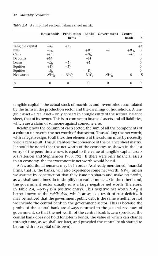
Table 2.4 A simplified sectoral balance sheet matrix

Households Production Banks Government Centralfirms bank �

Tangible capital +Kh +Kf +KBills +Bh +Bb −B +Bcb 0Cash +Hh +Hb −H 0Deposits +Mh −M 0Loans −Lh −Lf +L 0Equities +Ef −Ef 0Equities +Eb −Eb 0Net worth −NWh −NWf −NWb −NWg 0 −K

� 0 0 0 0 0 0

tangible capital – the actual stock of machines and inventories accumulatedby the firms in the production sector and the dwellings of households. A tan-gible asset – a real asset – only appears in a single entry of the sectoral balancesheet, that of its owner. This is in contrast to financial assets and all liabilities,which are a claim of someone against someone else.

Reading now the column of each sector, the sum of all the components ofa column represents the net worth of that sector. Thus adding the net worth,with a negative sign, to all the other elements of the column must by necessityyield a zero result. This guarantees the coherence of the balance sheet matrix.It should be noted that the net worth of the economy, as shown in the lastentry of the penultimate row, is equal to the value of tangible capital assetsK (Patterson and Stephenson 1988: 792). If there were only financial assetsin an economy, the macroeconomic net worth would be nil.

A few additional remarks may be in order. As already mentioned, financialfirms, that is, the banks, will also experience some net worth, NWb, unlesswe assume by construction that they issue no shares and make no profits,as we shall sometimes do to simplify our earlier models. On the other hand,the government sector usually runs a large negative net worth (therefore,in Table 2.4, −NWg is a positive entry). This negative net worth NWg isbetter known as the public debt, which arises as a result of past deficits. Itmay be noticed that the government public debt is the same whether or notwe include the central bank in the government sector. This is because theprofits of the central bank are always returned to the general revenues ofgovernment, so that the net worth of the central bank is zero (provided thecentral bank does not hold long-term bonds, the value of which can changethrough time, as we shall see later, and provided the central bank started tobe run with no capital of its own).

LAVOIE: “CHAP02” — 2006/9/11 — 10:01 — PAGE 33 — #11


2.3 The conventional income and expenditure matrix

2.3.1 The NIPA matrix

While the balance sheet matrix has its importance, the really interestingconstruct is the transactions flow matrix. This matrix records all the mone-tary transactions that are occurring in an economy. The matrix provides anaccounting framework that will be highly useful when defining behaviouralequations and setting up formal models of the economy. The transactionsmatrix is the major step in fully integrating income accounting and finan-cial accounting. This full integration will become possible only when capitalgains are added to the transactions matrix. When this is done, it will bepossible to move from the opening stocks of assets, those being held at thebeginning of the production period, to the closing stocks of assets, thosebeing held at the end of the production period.

But before we do so, let us consider the conventional income and expen-diture matrix, that is, the matrix that does not incorporate financial assets.This matrix arises from the consideration of the standard National Incomeand Product Accounts, the NIPA. We have already observed a very similarmatrix, when we examined the national accounts seen from the perspectiveof the standard mainstream macroeconomics textbook. Consider Table 2.5.Compared with the previous balance sheet matrix, the financial sector hasbeen scotched, amalgamated to the business sector, while the central bankhas been reunited with the government sector. We still have the double entryconstraint that the sum of the entries in each row ought to equal zero. Thisis a characteristic of all social accounting matrices.

It should be pointed out that all the complications that arise as a resultof price inflation, for instance the fact that the value of inventories mustbe adjusted to take into account changes in the price level of these inven-tories, have been assumed away. In other words, product prices are deemed

Table 2.5 Conventional Income and expenditure matrix

Business

Households Current Capital Government �

Consumption −C +C 0Govt expenditure +G −G 0Investment +I −If 0[GDP (memo)] [Y]Wages +WB −WB 0Net Profits +FD −F +FU 0Tax net of transfers −Th −Tf +T 0Interest payments +INTh −INTf −INTg 0

� SAVh 0 FU − If −DEF 0

LAVOIE: “CHAP02” — 2006/9/11 — 10:01 — PAGE 34 — #12


to remain constant. Unless we make this assumption we shall have to faceup, at far too early a stage, to various questions concerning the valuationof capital, both fixed and working, as well as price index problems. Thesecomplications will be dealt with starting with Chapter 8.

Before we start discussing the definition of gross domestic product, theperceptive reader may have noted that capital accumulation by householdsseems to have entirely disappeared from Table 2.5. It was already the case inTable 1.1, but then such an omission was tied to the highly simplified natureof the standard mainstream model, where only investment by firms was con-sidered. Why would investment in residential housing be omitted from amore complete NIPA? What happens is that, in the standard NIPA, automo-biles or household appliances purchased by individuals are not part of grosscapital formation; rather they are considered as part of current expenditures.In addition, to put home-owners and home-renters on an identical footing,‘home ownership is treated as a fictional enterprise providing housing ser-vices to consumer-occupants’ (Ruggles and Ruggles 1992 (1996: 284)). As aresult, purchases of new houses or apartments by individuals are assignedto fixed capital investment by the real estate industry; and expendituresassociated with home ownership, such as maintenance costs, imputed depre-ciation, property taxes and mortgage interest, ‘are considered to be expensesof the fictional enterprise’, and ‘are excluded from the personal outlays ofhouseholds’. In their place, there is an imputed expenditure to the fictional

AQ: Pleasecheck theinsertion ofclosing quoteafter the word‘households’and confirmwhether it isokay

real estate enterprise. This is why there is no Ih entry in Table 2.5 that wouldrepresent investment into housing.

2.3.2 GDP

In this matrix, the expenditure and income components of gross domesticproduct (GDP), appear in the second column. The positive and negative signshave a clear meaning. The positive items are receipts by businesses as a resultof the sales they make – they are the value of production – , while the negativeitems describe where these receipts ‘went to’: they are the product of theeconomy. It has been assumed that every expenditure in the definition ofGDP (consumption C, investment I , and government expenditures on goodsand services G) is a sale by businesses, although in reality this is not quitetrue, government employment – which is a form of expenditure which isnot a receipt by firms – being the major exception. And as a counterpart,every payment of factor income included in the income definition of GDP isa disbursement by businesses in the form of wages WB, distributed profits FDand undistributed profits FU, interest payments INTf , and indirect taxes Tf .From the second column, we thus recover the two standard definitions ofincome:

Y = C + I + G = WB + F + INTf + Tf (2.1)

LAVOIE: “CHAP02” — 2006/9/11 — 10:01 — PAGE 35 — #13


We must now confront the fact that firms’ receipts from sales of investmentgoods, which from the sellers’ point of view are no different from any otherkind of sales, do not arise from outside the business sector itself.7 So thedouble entry principle that regulates the use of accounting matrices requiresus to postulate a new sector – the capital account of businesses – which makesthese purchases. As we work down the capital account column, we shalleventually discover where all the funds needed for investment expenditurecome from.

There is no need to assume that all profits are distributed to householdsas is invariably assumed, without question, in mainstream macroeconomics.In the transactions matrix shown above, part of the net profits earned bybusiness are distributed to households (FD) while the rest is undistributed(FU) and (considered to be) paid into their capital accounts to be used as asource of funds – as it happens, the principal source of funds – for investment.Figure 2.1 shows that in the United States total internal funds of non-financialbusinesses exceeds their gross investment expenditures in nearly every year

19460.6

0.8

1

1.2

1.4

1.6

1.8

2

2.2

1951 1956 1961 1966 1971 1976 1981 1986 1991 1996 2001 2005

Total internal funds to Gross investment ratio

Figure 2.1 Total internal funds (including IVA) to gross investment ratio, USA,1946–2005.

Source: Z.1 statistics of the Federal Reserve, www.federalreserve.gov/releases/z1, table F102,Non-farm non-financial corporate business. The curve plots the ratio of lines 9 and 10.

7 As pointed out above, households’ investment in housing is imputed to the realestate industry.

LAVOIE: “CHAP02” — 2006/9/11 — 10:01 — PAGE 36 — #14


since 1946. In fact, it would seem that in many instances retained earningsare even used to finance the acquisition of financial assets.

To complete the picture, we include transfer payments between the varioussectors. These are divided into two categories, payments of interest (INT witha lower case suffix to denote the sector in question) that are made on assetsand liabilities which were outstanding at the beginning of the period andtherefore largely predetermined by past history; and other ‘unilateral’ trans-fers (T), of which the most important are government receipts in the formof taxes and government outlays in the form of pensions and other transferslike social insurance and unemployment benefits.

All this allows us to compute the disposable income of households –personal disposable income – which is of course different from GDP. It canbe read off the first column. Wages, distributed dividends, interest payments(from both the business and the government sector, minus interest paid onpersonal loans), minus income taxes, constitute this disposable income YD.8

YD = WB + FD + INTh − Th (2.2)

2.3.3 The saving = investment identity

Matrix 2.5 has now become a neat record of all the income, expenditure andtransfer payments which make up the national income accounts, showinghow the sectoral accounts are intertwined. The first column shows all cur-rent receipts and payments by the household sector, including purchases ofdurable goods, hence the balance at the bottom is equal to household saving(SAVh) as defined in NIPA. The second column shows current receipts andpayments by firms which defines business profits as the excess of receiptsfrom sales over outlays. The third column shows firms’ investment and theundistributed profits (FU) which are available to finance it, the balance atthe bottom showing the firms’ residual financing requirement – what theymust find over and above what they have generated internally. The entriesin the fourth column give all the outlays and receipts of the general govern-ment, and the balance between these gives the government’s budget surplusor deficit. The fact that every row until the bottom row, which describesfinancial balances, sums to zero guarantees that the balances’ row sums tozero as well. It is this last row which has attracted the undivided attention ofnational accountants and of Keynesian economists. This last line says that:

SAVh + (FU − If) − DEF = 0 (2.3)

Considering that the retained earnings of firms constitute the savings of thefirm’s sector, we can write FU = SAVf ; similarly, the surplus of the government

8 Note that interest payments from government are not included in GDP.

LAVOIE: “CHAP02” — 2006/9/11 — 10:01 — PAGE 37 — #15


sector is equivalent to its saving, so that SAVg = −DEF. From these newdefinitions, and from the definition implicit to the investment row, we canrewrite equation (2.3) in its more familiar form:

I = SAVh + SAVf + SAVg = SAV (2.4)

Equation (2.4) is nothing else than the famous Keynesian equality betweeninvestment and saving. This is the closest that most mainstream accountsof macroeconomics will get from financial issues.9 What happens to thesesavings, how they arise, what is their composition, how they link up thesurplus sectors to the deficit sectors, is usually not discussed nor modelled.In Matrix 2.5, until the final row, the nature of the transactions is pretty clear:households buy goods and firms sell them, etc.10 However, the transfer offunds ‘below the (bold) line’ requires a whole new set of concepts, which arenot part of the conventional income and expenditures national accounts.The answers to the questions that were put to the reader in section 1.2 ofthe previous section are to be found quite straight forwardly, using conceptswhich are familiar and easy to piece together so long as the double entryprinciple continues to be observed and so long as we always live up to ourmotto that everything must go somewhere and come from somewhere. Inother words, we need to bring in the transactions flow matrix.

2.4 The transactions flow matrix

2.4.1 Rules governing the transactions flow matrix

We shall require the reintroduction of the financial sector, the banks that hadbeen introduced in the balance sheet matrix but that had been amalgamated

9 Note that neo-classical economists don’t even get close to this equation, for other-wise, through equation (2.4), they would have been able to rediscover Kalecki’s (1971:82–3) famous equation which says that profits are the sum of capitalist investment,capitalist consumption expenditures and government deficit, minus workers’ saving.Rewriting equation (2.3), we obtain:

FU = If + DEF − SAVh

which says that the retained earnings of firms are equal to the investment of firmsplus the government deficit minus household saving. Thus, in contrast to neo-liberalthinking, the above equation implies that the larger the government deficit, the largerthe retained earnings of firms; also the larger the saving of households, the smaller theretained earnings of firms, provided the left-out terms are kept constant. Of course thegiven equation also features the well-known relationship between investment and prof-its, whereby actual investment expenditures determine the realized level of retainedearnings.

10 The nature of these transactions is not, in reality, so simple as this. In many,perhaps most cases, the contract to purchase and sell something is separated from thetransfer of money one way and the goods themselves going the other.

LAVOIE: “CHAP02” — 2006/9/11 — 10:01 — PAGE 38 — #16


to the business sector in the conventional income and expenditure matrix.Similarly, the operations of the central bank will reappear explicitly in thenew transactions flow matrix which is the corner stone of our approach.These additions to the conventional income and expenditure matrix willallow us to assess all transactions, be they in goods and services or in theform of financial transactions, with additions to assets or liabilities.

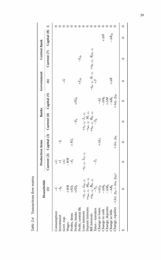
As in the balance sheet matrix, the coherence of the transactions flowmatrix is built on the rule that each row and each column must sum to zero.The rule enforcing that all rows must sum to zero is rather straightforward:each row represent the flows of transactions for each asset or for each kind offlow; there is nothing new here. The top part of the matrix, as described inTable 2.6 resembles the income and expenditure matrix, with a few additionsand new notations. In particular, the flow of interest payments, which wasnoted INT in Table 2.5, is now explicit. The flow of interest on an asset ora liability now depends on the relevant rate of interest and on the stock ofasset at the opening of the production period, that is, the stock accumulatedat the end of the previous period, at time t −1. The lagged variable rm standsfor the rate of interest prevailing on money deposits. Similarly rl and rb standfor the rates of interest prevailing on loans and Treasury bills.

The bottom part of the matrix is the flow equivalent of the balance sheetmatrix. When we describe purchases and sales of assets of which the nominalvalue never changes, there is no problem of notation. We simply write �Hor �M (for instance) to describe the increase in the stock of cash, or moneydeposits, between the beginning and end of the period being characterized.When the capital value of the asset can change – that is, when capital gainsand losses can occur, as is the case with long-term bonds and equities – wekeep the convention that the assets are pieces of paper, say e for equities,which have a price, pe. The value of the piece of paper is then e · pe at a pointof time, and the value of transactions in equities – new issues or buy-backs –is given by the change in the number of pieces of paper which are issued (orwithdrawn) times their price, �e · pe.

The rule enforcing that all columns, each representing a sector, must sumto zero as well is particularly interesting because it has a well-defined eco-nomic meaning. The zero-sum rule for each column represents the budgetconstraint of each sector. The budget constraint for each sector describes howthe balance between flows of expenditure, factor income and transfers gen-erate counterpart changes in stocks of assets and liabilities. The accounts ofthe transactions flow matrix, as shown by Table 2.6, are comprehensive inthe sense that everything comes from somewhere and everything goes some-where. Without this armature, accounting errors may pass unnoticed andunacceptable implications may be ignored. With this framework, ‘there areno black holes’ (Godley 1996: 7).

There is no substitute for careful perusal of the matrix at this stage. It is arepresentation, not easily come by, of a complete system of macroeconomic

LAVOIE: “CHAP02” — 2006/9/11 — 10:01 — PAGE 39 — #17

39

Tabl

e2.

6Tr

ansa

ctio

ns

flow

mat

rix

Pro

du

ctio

nfi

rms

Ban

ks

Go

vern

men

tC

entr

alB

ank

Ho

use

ho

lds

(1)

Cu

rren

t(2

)C

apit

al(3

)C

urr

ent

(4)

Cap

ital

(5)

(6)

Cu

rren

t(7

)C

apit

al(8

)�

Con

sum

pti

on−C

+C0

Inve

stm

ent

−Ih

+I−I

f0

Gov

t.ex

p.

+G−G

0W

ages

+WB

−WB

0Pr

ofits

,firm

s+F

Df

−Ff

+FU

f0

Profi

ts,b

anks

+FD

b−F

b+F

Ub

0Pr

ofit,

cen

tral

Bk

+Fcb

−Fcb

0Lo

anin

tere

sts

−rl(

−1)·L

h(−

1)−r

l(−1

)·L

f(−1

)+r

l(−1

)·L

(−1)

0D

epos

itin

tere

sts

+rm

(−1)

·Mh(−

1)−r

m(−

1)·M

(−1)

0B

ill

inte

rest

s+r

b(−1

)·B

h(−

1)+r

b(−1

)·B

b(−1

)−r

b(−1

)·B

(−1)

+rb(

−1)·B

cb(−

1)0

Taxe

s–

tran

sfer

s−T

h−T

f−T

b+T

0C

han

gein

loan

s+�

L h+�

L f−�

L0

Ch

ange

inca

sh−�

Hh

−�H

b+�

H0

Ch

ange

,dep

osit

s−�

Mh

+�M

0C

han

gein

bill

s−�

Bh

−�B

h+�

B−�

Bcb

0C

han

ge,e

qu

itie

s−(

�e f

·pef

+�

e b·p

eb)

+�e f

·pef

+�e b

·peb

0

�0

00

00

00

00

LAVOIE: “CHAP02” — 2006/9/11 — 10:01 — PAGE 40 — #18


transactions. The best way to take it in is by first running down each columnto ascertain that it is a comprehensive account of the sources and uses of allflows to and from the sector and then reading across each row to find thecounterpart of each transaction by one sector in that of another. Note thatall sources of funds in a sectoral account take a plus sign, while the uses ofthese funds take a minus sign. Any transaction involving an incoming flow,the proceeds of a sale or the receipts of some monetary flow, thus takes a pos-itive sign; a transaction involving an outgoing flow must take a negative sign.Uses of funds, outlays, can be either the purchase of consumption goods orthe purchase (or acquisition) of a financial asset. The signs attached to the‘flow of funds’ entries which appear below the horizontal bold line are stronglycounter-intuitive since the acquisition of a financial asset that would add to theexisting stock of asset, say, money, by the household sector, is described with anegative sign. But all is made clear so soon as one recalls that this acquisition ofmoney balances constitutes an outgoing transaction flow, that is, a use of funds.

2.4.2 The elements of the transactions flow matrix

Let us first deal with column 1 of Table 2.6, that of the household sector. Thatcolumn represents the budget constraint of the households. In contrast to thestandard NIPA, investment in housing is taken into account. Households canconsume goods (−C) or purchase new residential dwellings (−Ih), but only aslong as they receive various flows of income or provided they take in new loans(+�Lh) – consumer loans or home mortgages – or reduce their holdings ofassets, for instance by dishoarding money balances (+�Hh or +�Mh). At theaggregate scale, at least as a stylized fact, households add to their net wealth,through their saving. The excess of household income over consumption willtake the form of real purchases of dwellings (Ih), and the form of financialacquisitions: cash (�Hh), bank money (�Mh), fixed interest securities (�Bh),and equities (�e · pe), less the net acquisition of liabilities, in the form of loans(�Lh) from banks. The change in the net financial position of the householdsector, which will require counterpart changes in the net financial positionof the other sectors, appears in the rows below the bold line. The categoriesshown are simplified: there are other important ways in which people save –for example, through life insurance, mutual funds and compulsory pensionfunds; but for the time being these acquisitions will be treated as though theywere direct holdings, perhaps subject to advice from a manager.11

11 It has been shown by Ruggles and Ruggles (1992 (1996)) that once the fictitiousreal estate enterprises of NIPA that take care of households new purchases of residentialunits have been taken out, and once pension fund schemes are considered as saving byfirms rather than that of their employees, then the change in the net financial positionof the household sector is virtually nil, and even negative on the average in the UnitedStates since 1947.

LAVOIE: “CHAP02” — 2006/9/11 — 10:01 — PAGE 41 — #19


Column 2 is no different from the one discussed in Table 2.5: it showsthe receipts and the outlays of production firms on their current account.Column 3 now shows how production firms ultimately end up financingtheir capital expenditures, fixed capital and inventories. These capital expen-ditures, at the end of the period, appear to be financed by retained profits,new issues of securities (here assumed to be only equities, but which couldbe bonds or commercial paper) and bank loans.

Columns 4 and 5 describe a relatively sophisticated banking sector. Oncemore, the accounts are split into a current and a capital account. The currentaccount describes the flows of revenues and disbursements that the banksget and make. Banks rake in interest payments from their previous stocks ofloans and securities, and they must make interest payments to those holdingbank deposits. The residual between their receipts and their outlays, net oftaxes, is their profit Fb. This profit, as is the case for production firms, issplit between distributed dividends and retained earnings. These retainedearnings, along with the newly acquired money deposits, are the counterpartsof the assets that are being acquired by banks: new granted loans, newlypurchased bills, or additional vault cash. Column 5 shows how the balancesheets of banks must always balance in the sense that the change in theirassets (loans, securities and vault cash) will always have a counterpart in achange in their liabilities.

Finally, the last columns deal with the government sector and its cen-tral bank. The latter is split from the government sector, as it allows for amore realistic picture of the money creation process, although it adds oneslight complication. Let us first deal with Column 7, the current account ofthe central bank. From the balance sheet of Table 2.4, we recall that centralbanks hold government bills while their typical liabilities are in the form ofbanknotes, that is, cash, which carries no interest payment. As a result, cen-tral banks make a profit, Fcb, which, we will assume, is entirely returned togovernment. This explains the new entry in column 6 of the governmentsector, +Fcb, compared with that of Table 2.5. The fact that the central bankreturns all of its profits to government implies that the while the govern-ment gross interest disbursements on its debt are equal to rb(−1) · B(−1), itsnet disbursements are only rb(−1) · [B(−1) − Bcb(−1)].

Column 6 is the budget constraint of government. It shows that any gov-ernment expenditure which is not financed by taxes (or the central bankdividend), must be financed by an issue of bills. These newly issued billsare purchased by households, banks and the central bank, directly or indi-rectly. Column 8 shows the highly publicized accounting requirement thatany addition to the bond portfolio of the central bank must be accompaniedby an equivalent increase in the amount of high-powered money, +�H . Thisrelationship, which is at the heart of the monetarist explanation of inflation –also endorsed by most neo-classical economists – as proposed by authors suchas Milton Friedman, has been given considerable attention in the recent past,

LAVOIE: “CHAP02” — 2006/9/11 — 10:01 — PAGE 42 — #20


since it seems to imply that government deficits are necessarily associatedwith high-powered money increases, and hence through some money mul-tiplier story, as told in all elementary textbooks, to an excess creation ofmoney. A quite different analysis and interpretation of these accountingrequirements will be offered in the next chapters.

2.4.3 Key features of the transactions flow matrix

It is emphasized that so far there has been no characterization of behaviourbeyond what is implied by logical constraints (e.g. that every buyer musthave a seller) or by the functions that have been allocated to the varioussectors (e.g. that firms are responsible for all production, banks for makingall loans) or by the conventional structure and significance of asset portfolios(e.g. that money is accepted as a means of payment).

Reconsider now the system as a whole. We open each period with stocksof tangible assets and a tangle of interlocking financial assets and liabilities.The whole configuration of assets and liabilities is the legacy of all transac-tions in stocks and flows and real asset creation during earlier periods whichconstitute the link between past, present and future. Opening stocks inter-act with the transactions which occur within each period so as to generate anew configuration of stocks at the end of each period; these will constitutepast history for the succeeding period. At the aggregate level, whatever isproduced and not consumed will turn up as an addition to the real capitalstock. At the sectoral level, the sum of all receipts less the sum of all outlaysmust have an exact counterpart in the sum of all transactions (by that sector)in financial assets less financial liabilities.

The only elements missing for a full integration are the capital gains thatought to be added to the increases in assets and liabilities that were assessedfrom the transactions matrix. Thus what is missing is the revaluation account,or what is also known as the reconciliation account. When this is done, itbecomes possible to move from the opening stocks of assets, those beingheld at the beginning of the production period, to the closing stocks of assets,those being held at the end of the production period. This will be done inthe next section.

The system as a whole is now closed in the sense that every flow and everystock variable is logically integrated into the accounting to such a degreethat the value of any one item is implied by the values of all the otherstaken together; this follows from the fact that every row and every columnsums to zero. This last feature will prove very useful when we come to modelbehaviour; for however large and complex the model, it must always be thecase that one equation is redundant in the sense that it is implied by all theother equations taken together.

As pointed out in the first part of this chapter, other authors have previ-ously underlined the importance of the transactions flow matrix. In his book,Jean Denizet (1969: 19) proposed a transactions flow matrix that has implicitly

LAVOIE: “CHAP02” — 2006/9/11 — 10:01 — PAGE 43 — #21


all the features of the matrix that has been presented here. Malinvaud (1982:21) also presents a nearly similar transactions flow matrix. The article writtenby Tobin and his collaborators (Backus et al. 1980), has a theoretical transac-tion flow matrix, nearly identical to the one advocated here, with rows andcolumns summing to zero; they also have presented the empirical version ofsuch a matrix, including capital gains, with actual numbers attached to eachcell of our transaction flow matrix, derived from the national income andproduct accounts and the flow-of-funds accounts, thus demonstrating thepractical usefulness of this approach. The transactions flow matrix has beenutilized systematically and amalgamated to behavioural equations by Godleyin his more recent work (1996, 1999a). It was not present in Godley’s earlierwork (Godley and Cripps 1983).

2.5 Full integration of the balance sheet andthe transactions flow matrices

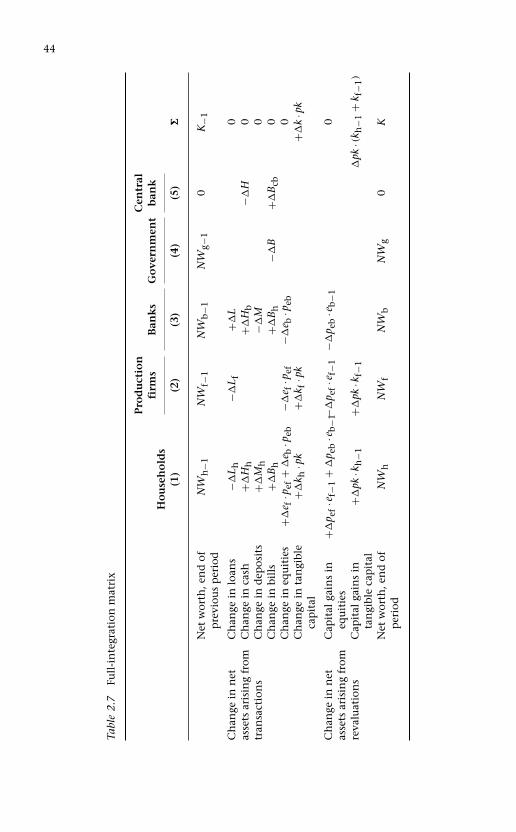
We are now in a position to integrate fully the transactions flow matrix tothe balance sheet. Table 2.7 illustrates this integration (Stone 1986: 16). Asbefore, we consider five sectors: households, production firms, banks, gov-ernment, and the central bank. The first row represents the initial net worthof each sector, as they appear in the penultimate row of Table 2.6. We assumeagain that the net worth of the central bank is equal to nil, as a result of thehypothesis that any profit of the central bank is returned to government. Weshall also see that a central bank zero net worth requires that the central bankholds no bonds, only bills, the price of which does not change. We may alsonote, as was mentioned earlier, that the aggregate net worth of the economy,its macroeconomic net worth, is equal to the value of tangible capital, K.Finally, it should be pointed out once more that the net worth of any sector,at the end of the previous period, is considered to be the same thing as the networth of that sector at the beginning of the current period, and in what followswe shall make use of the (−1) time subscript whenever beginning-of-periodwealth is referred to.

The change in the net worth of any sector is made up of two components,as is clearly indicated in the first column of Table 2.7: the change in net assetsarising from transactions, and the change arising from revaluations, that is,changes in the prices of assets or liabilities. These two components of change,added to the net worth of the previous period, yield the new net worth ofeach sector. This new net worth – the net worth at the end of the currentperiod – appears in the last row of Table 2.7.

The first component of the change in net worth arises from the transactionsflow matrix. The first five rows of these changes are the exact equivalent of thelast five rows (the last row of zeros having been set aside) of the transactionsflow matrix 2.6. They reflect the financial transactions that occurred during

LAVOIE: “CHAP02” — 2006/9/11 — 10:01 — PAGE 44 — #22

44

Tabl

e2.

7Fu

ll-i

nte

grat

ion

mat

rix

Pro

du

ctio

nC

entr

alfi

rms

Ban

ks

Go

vern

men

tb

ank

Ho

use

ho

lds

(1)

(2)

(3)

(4)

(5)

�

Net

wor

th,e

nd

ofp

revi

ous

per

iod

NW

h−1

NW

f−1

NW

b−1

NW

g−1

0K

−1

Ch

ange

inn

etC

han

gein

loan

s−�

L h−�

L f+�

L0

asse

tsar

isin

gfr

omC

han

gein

cash

+�H

h+�

Hb

−�H

0tr

ansa

ctio

ns

Ch

ange

ind

epos

its

+�M

h−�

M0

Ch

ange

inbi

lls

+�B

h+�

Bh

−�B

+�B

cb0

Ch

ange

ineq

uit

ies

+�e f

·pef

+�

e b·p

eb−�

e f·p

ef−�

e b·p

eb0

Ch

ange

inta

ngi

ble

+�k h

·pk

+�k f

·pk

+�k

·pk

cap

ital

Ch

ange

inn

etC

apit

alga

ins

in+�

p ef·e f

−1+

�p e

b·e b

−1−�

p ef·e f

−1−�

p eb

·e b−1

0as

sets

aris

ing

from

equ

itie

sre

valu

atio

ns

Cap

ital

gain

sin

+�pk

·kh−1

+�pk

·kf−

1�

pk·(k

h−1

+k f

−1)

tan

gibl

eca

pit

alN

etw

orth

,en

dof

NW

hN

Wf

NW

bN

Wg

0K

per

iod

LAVOIE: “CHAP02” — 2006/9/11 — 10:01 — PAGE 45 — #23


the period. The only difference between these five rows as they appear inTable 2.7 compared to those of Table 2.6 is their sign. All minus signs inTable 2.6 are replaced by a plus sign in Table 2.7, and vice versa. In thetransactions flow matrix of Table 2.6, the acquisition of a financial asset, saycash money �Hh by households, is part of the use of funds, and hence carriesa minus sign. However, in Table 2.7, the acquisition of this cash money addssomething to household wealth, and hence it must carry a plus sign, in orderto add it to the net worth of the previous period. Similarly, when householdsor firms take loans, these new loans provide additions to their sources of funds,and hence carry a plus sign in the transactions flow matrix of Table 2.6. Bycontrast, in the integration matrix of Table 2.7, loans taken by householdsor firms, all other things equal, reduce the net worth of these sectors, andhence must carry a minus sign.

The last element of the first block of six rows arising from the transactionsflow matrix, as shown in Table 2.7, is the row called ‘change in tangiblecapital’. The counterpart of this row can be found in the ‘investment’ rowof Table 2.6. Households, for instance, can augment their net wealth byacquiring financial or tangible capital. In their case, tangible capital is essen-tially made up of residential dwellings (since, in contrast to financial flowsaccountants, we do not consider purchases of durable goods as capital accu-mulation). This was classified as investment in the transactions flow matrix,and called Ih, whereas in the full-integration matrix, it is called �kh · pk,where pk is the price of tangible capital, while �kh is the flow of new residen-tial capital being added to the existing stock, in real terms. In other words,�kh is the number of new residential units which have been purchased byhouseholds. It follows that we have the equivalence, Ih = �kh · pk. Similarly,for firms, their investment in tangible capital (essentially machines, plants,and additions to inventories) was called If in the transactions matrix of Table2.6. Setting aside changes in inventories,12 the value of new investment in tan-gible capital is now called �kf · pk in Table 2.7, so that we have the otherequivalence, If = �kf · pk. Note that for simplification, we have assumed thatthe price of residential tangible capital and the price of production capital isthe same and moves in tandem.

The second major component of the change in net worth arises from capitalgains. For exposition purposes, we assume that only two elements of wealthcan have changing prices, and hence could give rise to capital gains or capitallosses. We assume that the prices of equities can change, those issued byproduction firms and those issued by banks; and we also assume that the

12 This is an important restriction, because, as already pointed out, inventories arevalued at current replacement cost, while fixed capital is valued at current replacementprice, and hence they cannot carry the same price variable. See Chapter 11 for anin-depth study of this issue, which is briefly dealt with in section 2.6.2.

LAVOIE: “CHAP02” — 2006/9/11 — 10:01 — PAGE 46 — #24


price of tangible capital, relative to consumer prices, can change. We assumeaway changes in the price of securities. The implicit assumption here is thatall securities are made up of bills – short-term securities that mature withinthe period length considered here. In the case of bonds – long-term securitiesthe prices of which change from period to period, before they mature andcome up for redemption – capital gains or losses would have to be taken intoaccount. Capital gains on bonds will be explicitly taken into considerationin Chapter 5.

The study of capital gains underlines an important principle: any changein the value of an asset may be made up of two components: a componentassociated with a transaction, for instance when new equities are issued andbought up for instance, thus involving additional units of the asset in ques-tion; and a component associated with a change in the price of the asset,when for instance, existing (and newly issued) equities carry a higher price.In the case of equities issued by production firms, as shown in Table 2.7,the change in the value of equities arising from transactions is �ef · pef whilethe change in the value of equities arising from capital gains is �pef · ef−1. InChapter 5, we shall provide a precise proof of this result in discrete time (withtime subscripts, as done here). In the meantime, it is sufficient to remem-ber first-year university calculus, deal with continuous time, and recall that,given two functions, u and v, the derivative of the product of these functionsis such that d(u · v) = du · v + u · dv. In the present case, with e and pe actingas the two functions u and v, we have:

d(e · pe) = de · pe + e · d(pe) (2.5)

The first term represents the change arising from transactions, while thesecond term represents capital gains due to the change in prices. The samerules apply to the changes in the value of tangible capital, where a real termcomponent and a price component can be identified.

Thus, adding the capital gains component so defined and the transac-tions component to the net worth of the previous period, we obtain thenet worth at the end of the current period, as shown in the last row ofTable 2.7. The integration of the flow of funds financial transactions andthe sector balance sheets with the national income accounts is thus com-plete. It should be pointed out however that it is no easy matter to producean empirical version of Tables 2.6 or 2.7. While the flow of funds publishedby the Federal Reserve in the United States, or by other statistical agencies inother countries, contain a vast amount of information about transactions infinancial assets, the sectoral classification and to some extent the conceptsemployed in NIPA are sufficiently different to make any simple junctionof the two data sets. Although the Z.1 accounts themselves provide somereconciliation (in tables F.100 and higher), relatively large discrepanciesremain.

LAVOIE: “CHAP02” — 2006/9/11 — 10:01 — PAGE 47 — #25


2.6 Applications of the transactions flow matrix:the monetary circuit

2.6.1 The quadruple-entry principle and productionwith private money

It has already been claimed that the transactions flow matrix serves animportant purpose in guaranteeing the coherence of the accounting whenmacroeconomic models are built. But the transactions flow matrix can alsobe shown to serve a further purpose. The transactions flow matrix canreally help us to understand how production is being financed at the ini-tial finance state, that is at the beginning of the production period, beforehouseholds have decided on what they will do with their newly acquiredincome or their newly acquired savings. The transactions flow matrix sets themonetary circuit – about which so much has been said by French and Ital-ian post-Keynesian school, the so-called circuitistes – within a comprehensiveaccounting framework, which will help to justify the story told and the claimsmade by these post-Keynesians (Graziani 1990). In other words, the transac-tions flow matrix, which ties together real decisions and monetary and finan-cial consequences, is the backbone of the monetary production economy thatKeynes and his followers, the post-Keynesians, wish to describe and to model.To get a feel for how the system works we may follow through a few transac-tions as though they were sequences. We will examine two of these transac-tions. First, we shall look at how the production of firms is being financed;then we shall see how government expenditures enter the economy.

Suppose, as we assumed in the transactions flow matrix, that firmsdistribute wages in line with production, that dividends are distributedaccording to past profits, and that interest payments, as shown here, dependson the past stock of deposits and on a rate of interest administered by thebanking system. Suppose further that firms borrow, at the beginning of theproduction period as the circuitistes would have it, the amount needed topay the wages of the current period. This is, as the circuitistes say, the firststep of the monetary circuit (Lavoie 1992: 153). Thus in the first step of thecircuit, both the loans and the deposits newly created by the banking systembelong to the production sector. This initial step of the monetary circuit withprivate money is shown in Table 2.8A, which is a subset of the transactionsmatrix of Table 2.6.

A clear feature of Table 2.8A. is that it contains four entries. This is an illus-tration of the famous quadruple-entry system of Copeland (1949 (1996: 8)).Copeland pointed out that, ‘because moneyflows transactions involve twotransactors, the social accounting approach to moneyflows rests not on adouble-entry system but on a quadruple-entry system’. Knowing that eachof the columns and each of the rows must sum to zero at all times, it followsthat any alteration in one cell of the matrix must imply a modification toat least three other cells. The transactions matrix used here provides us with

LAVOIE: “CHAP02” — 2006/9/11 — 10:01 — PAGE 48 — #26


Table 2.8A First step of the monetary circuit with private money

Production firms Banks

Households Current A. Capital A. Capital A. �

ConsumptionInvestmentWages� loans + �Lf −�L 0� deposits −�Mf +�M 0

� 0 0 0

an exhibit which allows to report each financial flow both as an inflow to agiven sector and as an outflow to the other sector involved in the transaction.In the current instance, the production and the banking sectors are the twoparties to the financial transaction, and each sector must have two modifiedentries, since all columns must balance.

A peculiar feature of the quadruple-entry system is that it corrects a preva-lent misconception regarding the creation and the role of money. In themainstream framework, money is sometimes said to fall from the sky, thrownout of an helicopter, as in the famous parable by Milton Friedman. In thatmainstream framework, which is highly popular in mainstream interme-diate macroeconomic textbooks, money is a given stock, which seems toappear from nowhere, and which has no counterpart in the rest of theeconomy. Despite changes in the real economy, and presumably in finan-cial flows, the stock of money is assumed to remain at all time constant.The quadruple-entry system shows that such a conception of money ismeaningless.

Coming back to Table 2.8A, a very important point, related to the dan-gers of confusing semantics, must be made. Recall that a minus sign in thetransaction matrix is associated with the use of funds, while a positive signimplies the source of funds. In Table 2.8A, in the column of banks, the addi-tion to money deposits is associated with a plus sign, while the addition tobank loans is associated to a minus sign. From a flow-of-funds standpoint,increased deposits are thus a source of funds while increased loans are a useof funds for the banks. For some, this terminology seems to reinforce themainstream belief, associated with the loanable funds approach, that banksprovide loans only insofar as they have the financial resources to do so; inother words, banks make loans only when they have prior access to deposits.The source of the funds to be lent, in Table 2.8A, is the money deposits, asthe minus sign would show.

Needless to say, this loanable funds interpretation is not being defendedhere. On the contrary, a key feature of the banking system is its ability to

LAVOIE: “CHAP02” — 2006/9/11 — 10:01 — PAGE 49 — #27


create deposits ex nihilo. More precisely, when agents in the economy arewilling to increase their liabilities, banks can increase the size of both sides oftheir balance sheet, by granting loans and simultaneously creating deposits.As neatly summarized by Earley, Parsons and Thomson (1976, 1996: 159), ‘toencapsulate, we see fluctuations in borrowing as the primary cause of changesin spending’. It may be that, in flow-of-funds terminology, money depositsis the source of funds allowing the use of bank loans. But the cause of thisincrease in deposits and loans is the willingness to contract an additionalliability and the desire of the borrower, here the production firm, to expandits expenditures.

2.6.2 Initial finance versus final finance

This situation as shown in Table 2.8A, however, can only last for a splitsecond. Firms only draw on their lines of credit when they are required tomake payments. In the second step of the circuit, the deposits of the firms aretransferred by cheques or electronic payment to the workers who providedtheir labour to the firms. The moment these funds are transferred, they con-stitute households’ income. Before a single unit is spent on consumer goods,the entire amount of the bank deposits constitutes savings by households,and these are equal to the new loans granted to production firms.

This is all shown in Table 2.8B. The matrix requirement that all rows andcolumns must sum to zero makes clear the exigencies of the second step ofthis monetary circuit. Because of these zero-sum requirements, the followingthree equations must hold:

I − WB = 0 (2.6)

I − �Lf = 0 (2.7)

�Mh − �Lf = 0 (2.8)

At that stage of the circuit, output has been produced but not yet sold. Theunsold production constitutes an increase in inventories (which will later be

Table 2.8B The second step of the monetary circuit with private money

Production firms Banks

Households Current A. Capital A. Capital A. �

ConsumptionInvestment +I −I 0Wages +WB −WB 0� loans +�Lf −�L 0� deposits −�Mh +�M 0� 0 0 0 0 0

LAVOIE: “CHAP02” — 2006/9/11 — 10:01 — PAGE 50 — #28


associated with the symbol IN). This increase in inventories is accounted asinvestment in working capital. Staying faithful to our requirement that allrows and all columns must sum to zero, inventories must necessarily riseby an amount exactly equal to the production costs, the wages paid WB,as in equation (2.6).13 The zero-sum column requirement, as applied to thecurrent account of firms makes it so. This demonstrates a very importantpoint: that inventories of unsold goods should be valued at cost, and notaccording to the price that the firm believes it can get for its goods in thenear future.

On the side of the capital account, it is clear that the value of this invest-ment in inventories must be financed by the new loans initially fetched for, asin equation (2.7). Table 2.8B, contrasted with Table 2.6, helps to understandthe distinction between initial and final finance which has been underlined bythe circuitistes (Graziani 1990). Initial finance, or what Davidson (1982: 49)calls construction finance, appears in Tables 2.8A: it is the bank loans that firmsusually ask to finance the initial stages of production and hence to financeinventories. Final finance, or Davidson’s investment funding, is to be foundin the last rows of Table 2.6. Final finance are the various means by whichinvestment expenditures are being ultimately financed by the end of the pro-duction period; the retained earnings of corporations constitute the greatestpart of gross investment funding.

The transition from Tables 2.8A and 2.8B, which represent the first andsecond steps of the monetary circuit, to Table 2.6, which represents the thirdand last step of the monetary circuit, is accomplished by households gettingrid of the money balances acquired through wages, and eventually the addi-tional money balances received on account on their dividend and interestpayments. As the households get rid of their money balances, firms gradu-ally recover theirs, allowing them to reimburse the additional loans that hadbeen initially granted to them, at the beginning of the period.

The key factor is that, as households increase their consumption, theirmoney balances fall and so do the outstanding amount of loans owed by thefirms. Similarly, as households get rid of their money balances to purchasenewly issued equities by firms, the latter are again able to reduce their out-standing loans. In other words, at the start of the circuit, the new loansrequired by the firms are exactly equal to the new deposits obtained byhouseholds. Then, as households decide to get rid of their money balances,the outstanding loans of firms diminish pari passu, as long as firms use theproceeds to pay back loans instead of using the proceeds to beef up theirmoney balances or their other liquid financial assets. Although determinedby apparently independent mechanisms, the supply of loans to firms and

13 Note that it is assumed as well that the new fixed investment goods have not yetbeen sold to the corporations which ordered them.

LAVOIE: “CHAP02” — 2006/9/11 — 10:01 — PAGE 51 — #29


the holdings of deposits by households (and firms) cannot but be equal, asthey are at the beginning of the circuit, as in equation (2.8). This mechanismwill be observed time and time again in the next chapters, when behaviouralrelations are examined and formalized.

The primary act is best thought of as a decision to produce something.This induces firms to take up a loan to start up the production process. Thebuild up of initial inventories, when production begins, is the result of such aproduction decision, made with the agreement of a bank. It is this act whichbrings a bank loan into existence and simultaneously brings a bank balanceof equal size into existence (that of the firm asking for a loan). As soon ashouseholds are paid for their services, the money deposits are transferred tothe bank accounts of the newly employed labour force.14 We can already seehow it is that the household sector comes to ‘lend’ its surplus to the produc-tion sector, as mainstream economists would say. In the example just given,the mere holding of the money paid out as wages has a loan as its exactcounterpart. When the household sector buys something from the produc-tion sector, this destroys money and loans by an exactly equal amount. Whilethe loan-granting activity created an efflux of money into the economy, thepurchase of goods by households creates a reflux – the destruction of money.Thus, any series of transactions can be conceived as the creation, circulationand destruction of money.

2.6.3 Production with central bank money

The steps of the monetary circuit can once again be used to help understandhow money creation and government deficits are being related to each other.Suppose that, at the beginning of the circuit, the government sector ordersthe production of some goods to the private production sector. Once thesegoods have been produced, they must be purchased by government. Thesimplest solution to do so would be for government to draw on its line ofcredit at the central bank: the government sector would get high-poweredmoney as the central bank would grant a loan to its government. But suchcredit facilities are now regarded as inflationary by mainstream economistsand politicians, and as a result, these direct credit facilities are forbidden bylaw. The alternative is for government to issue new bills, which can eitherbe purchased by the central bank or by a private bank. Direct governmentbond sales to the central bank are also feared by mainstream economists, andas a result, in some countries, they are either forbidden or highly restricted.But let us assume that such a sale occurs anyway. The counterpart of thenewly purchased bills, in the books of the central bank, is the amount ofhigh-powered money credited to the government account. This is, once

14 There is some resemblance with Moore’s (1997: 426) point that ‘depositors canonly “supply” banks with deposits if they have somehow previously acquired them’.

LAVOIE: “CHAP02” — 2006/9/11 — 10:01 — PAGE 52 — #30


more the first step of the monetary circuit, and it is shown with the help ofTable 2.9A. This money will circulate, first to pay the producing firms. Thesefirms get cheques, drawn on the account of the government sector at the cen-tral bank. Once cashed at the private banks, these cheques give rise to bankdeposits. This is shown in Table 2.9B. The firms then use these bank depositsto pay their workers and remunerate their owners. Here for simplification,the income so created is to be found on a single row, as Y .15 The moneybalances so created will thus wind up in the deposit accounts of households.This is illustrated with the help of Table 2.9C.

Table 2.9A The first step of government expenditures financed by central bank money

Production Centralfirms Banks bank

Households Current Capital Government Capital �

Govt. exp.Income [GDP]Change in cash −�Hg +�H 0Change in deposits 0Change in bills +�B −�Bcb 0

� 0 0 0

Table 2.9B The second step of government expenditures financed by central bankmoney



Govt. exp. +G −G 0Income [GDP]Change in cash −�Hb +�H 0Change in deposits −�Mf + �M 0Change in bills +�B −�Bcb 0

� 0 0 0 0 0

15 Here we have slightly cheated, assuming that all profits are distributed tohouseholds.

LAVOIE: “CHAP02” — 2006/9/11 — 10:01 — PAGE 53 — #31


Table 2.9C The third step of government expenditures financed by central bankmoney



Govt. exp. +G −G 0Income [GDP] +Y −Y 0Change in cash −�Hb +�H 0Change in deposits −�Mh +�M 0Change in bills +�B −�Bcb 0

� 0 0 0 0 0 0

Once again, all rows and columns must sum to zero. Before households decidewhat to do with their newly acquired money balances, spending them onconsumption or acquiring interest-earning assets – including governmentbills –, all accounts must balance. As a consequence, the deficit cannot butbe ‘monetized’ initially, in line with what neo-chartalist post-Keynesianshave been recently arguing (Wray 1998: ch. 4–5; Mosler and Forstater 1999).The matrices of Tables 2.9B and 2.9C also show the standard result, so oftenunderlined in mainstream textbooks, that private banks now wind up withadditional reserves, the �Hb entry in the capital account of banks. These extrareserves do not mean however that a multiple amount of money depositswill be created, as the standard money multiplier has it. If banks do not findany credit-worthy borrower – and the fact that they now have additionalreserves implies in no way that additional credit-worthy borrowers will beforthcoming – they always have the choice to purchase government bills.16

As we shall see more formally in Chapter 4, if the central bank is to keep theinterest rate at its target level, the central bank must sell to the banks (andto households) the bills that they lurk for, and by so doing, the central bankwill absorb the money balances that neither the banks nor the householdswish to hold.

We said before that the government sector, to finance its expenditures,could also have sold its bills to private banks. The transactions matrix thatcorresponds to such a transaction, with the ensuing deposits ending up inthe hands of workers and stockholders is even simpler, as illustrated withthe help of Tables 2.10A and 2.10B. Private banks buy the bills and granta bank deposit to the government, as shown in Table 2.10A. This depositthen moves on to the household sector, after having transited through the

16 There is another possibility that will be examined in the next subsection.

LAVOIE: “CHAP02” — 2006/9/11 — 10:01 — PAGE 54 — #32


Table 2.10A The first step of government expenditures financed by private money



Govt. exp.Income [GDP]Change in cashChange in deposits +�M −�Mg 0Change in bills −�Bb +�B 0

� 0 0 0

Table 2.10B The third step of government expenditures financed by private money



Govt. exp. +G −G 0Income [GDP] +Y −Y 0Change in cashChange in deposits −�Mh +�M 0Change in bills −�Bb +�B 0

� 0 0 0 0 0 0

production sector, when the public goods are paid for. This is shown withthe help of Table 2.10B. It would seem this time that there is no inflationarydanger, since banks hold no additional high-powered money, in contrast tothe case where bills were being purchased directly by the central bank. Butthis is all an illusion. Whether the bills are initially purchased by banks orby the central bank makes no difference whatsoever. If banks or householdsare in need of additional cash, as a consequence of the increased activitygenerated by the public expenditures, the central bank will need to intervenein the second-hand market, purchasing some of the bills initially bought bythe private banks, as long as it wishes to maintain its interest rate target.In the end, the only money or high-powered money left in the economywill be held voluntarily, and this amount depends in no way on the exactfinancial scheme used to finance government expenditures.

LAVOIE: “CHAP02” — 2006/9/11 — 10:01 — PAGE 55 — #33


2.6.4 The case of the overdraft economy

Up to now, we have assumed that government expenditures were financedeither by selling bonds to the private banks, or by selling bonds to the cen-tral bank. This corresponds however to a particular institutional set-up, thatHicks (1974: 51) has called the pure auto-economy. It turns out however thatthe pure auto-economy, or what Lavoie (2001b: 216) has called the asset-basedeconomy, is only one of the possible institutional set-ups. While the asset-based economies have been described in great detail in mainstream text-books, specially in Anglo-saxon textbooks, the other institutional set-upshave been usually ignored. It turns out, however, that most financial systemsin the world are not of the asset-based type, but rather can be described as

Table 2.11A First step of government expenditures in overdraft system



Govt. exp.Income [GDP]Change in cashChange in deposits +�M −�Mg 0Change in bank loans −�L +�Lg 0Change in central

bank advances

� 0 0 0

Table 2.11B Second step of government expenditures in overdraft system



Govt. exp. +G −G 0Income [GDP] +Y −Y 0Change in cash −�Hh +�H 0Change in deposits −�Mh +�M 0Change in bank loans −�L +�Lg 0Change in centralbank advances

+�A −�A 0

� 0 0 0 0 0 0

LAVOIE: “CHAP02” — 2006/9/11 — 10:01 — PAGE 56 — #34


overdraft economies, making use once more of the terminology proposed byHicks (1974: 53).

In the pure overdraft economy, as defined by Hicks, firms hold no financialassets, and are thus ‘wholly dependent, for their liquidity, on the banks’. Thenotion of a pure overdraft economy can however be extended to the relationsbetween the private banks and the central bank, as is done in Lavoie (2001b).In pure overdraft financial systems, private banks hold little or no govern-ment securities. On the contrary, private banks in such overdraft economiesare permanently in debt vis-á-vis the central bank, having borrowed fundsfrom the central bank to acquire the reserves that they are legally requiredto hold, and to obtain the central bank banknotes that their customers havebeen asking for.

The impact of new government expenditures on the transactions flowmatrix, or at least a part of it, is shown in Tables 2.11A and 2.11B. As before,we assume new government expenditures of an amount G. This is nowfinanced by a loan from the private banks to the government. This is shown inTable 2.11A, which is very similar to Table 2.8A. These government expendi-tures generate an income of Y , which we assume as before to be kept initiallyin the form of money balances by households. A new assumption, comparedto Tables 2.9 or 2.10, is that households wish to hold a certain portion oftheir new money balances in the form of cash money. In the pure overdrafteconomy, private banks must borrow all cash money from the central bank.Private banks obtain advances A from the central bank, to cover the needsin cash money of the public, as shown in Table 2.11B. Within such a systemwithout government securities, the determination of interest rates is quitestraightforward. The central bank simply needs to set the rate of interest onthe advances made to private banks. This rate of interest on advances is thenthe base rate of interest, that sets the standard for all other rates of interestin the financial system. The study of overdraft financial systems thus helpto pierce through the veil of the asset-based financial systems, showing withobvious simplicity that central banks do have the ability to set short-terminterest rates.

Documents

Balance Sheets, Transaction Matrices and the Monetary … Lavoie 2007 chap02 … · · 2010-06-03Balance Sheets, Transaction Matrices and the Monetary Circuit ... consumption, accumulation