Embed Size (px)
Citation preview

1
Bailout Policies and Banking Risk in Crisis Periods
Ramon S. Vilarins**
Rafael F. Schiozer*
Abstract: This paper analyzes the impact of government bailout policies on the risk of the
banking sector in OECD countries between 2005 and 2013. First, in line with the moral
hazard hypothesis, we verify that financial institutions with high bailout expectations assume
higher risks than others. Second, we find that, in normal times, rescue guarantees to large
financial institutions distort competition in the sector and increase the risk of the other
institutions. However, during the recent financial crisis, increases in the rescue expectation of
competitors of an institution, to the extent that they represent a reduction in its chance of
bailout, decrease its risk taking. Additionally, in a crisis period, it is also evident that the
deterioration in the countries’ sovereign capacity to bailout banks is associated with lower
risk taking; on average, the increase in risk taking is higher in countries with a lower credit
default swap spread.
Keywords: bank bailout, bank risk taking, bank competition, financial crisis
JEL Classification: G210, G320, G010
** Banco Central do Brasil and Fundação Getulio Vargas – EAESP. The opinions expressed herein are those of
the authors and not necessarily those of the Banco Central do Brasil (Central Bank of Brazil). E-mail:
* Fundação Getulio Vargas – EAESP. E-mail: [email protected].

2
BAILOUT POLICIES AND BANKING RISK IN CRISIS PERIODS
Abstract: This paper analyzes the impact of government bailout policies on the risk of the
banking sector in OECD countries between 2005 and 2013. First, in line with the moral
hazard hypothesis, we verify that financial institutions with high bailout expectations assume
higher risks than others. Second, we find that, in normal times, rescue guarantees to large
financial institutions distort competition in the sector and increase the risk of the other
institutions. However, during the recent financial crisis, increases in the rescue expectation of
competitors of an institution, to the extent that they represent a reduction in its chance of
eventual government bailout, decrease its risk taking. Additionally, in a crisis period, it is
also evident that the deterioration in the countries’ financial conditions are associated with
lower risk taking; on average, the increase in risk taking is higher in countries with a lower
credit default swap spread.
1 Introduction
The expansion of the banking safety net is often used in the management of financial crises.
However, there is still no consensus in the literature with regard to the ex-ante and ex-post
effects on bank risk taking. Under the hypothesis of market discipline, the safety net reduces
the incentive for depositors, creditors, and shareholders to monitor the behavior of financial
institutions (FIs), thereby leading to an increase in their risk level (Flannery, 1998). In turn,
the charter value hypothesis states that government guarantees make banks more conservative
(Keeley, 1990). Bailout expectations are higher for a select group (too big to fail, or
systemically important) of banks. Oliveira, Schiozer and Barros (2015) shows that this policy
distorts competition by allowing these banks increased access to liquidity when it is most
scarce, and Gropp, Hakenes and Schnabel (2011) shows that competition distortions causes
unprotected banks to take even more risk.
A number of recent studies examine the risk taking of banks and the banking safety net in
periods of financial stress (e.g., Damar, Gropp and Mordel (2012); Acharya, Drechsler and
Schnabl (2014), among others). These studies suggest that the incentives for bank risk taking

3
(i.e., the variables that affect risk taking) in normal times are different from those in a
financial crisis.
This study investigates whether the bailout expectation affects the level of bank risk both in
normal times and during financial crises. Since the theory suggests that bailout expectations
may either increase or decrease bank risk, the relative magnitude of the forces that drive bank
risk may be different in normal times and during the financial crisis. Beyond that, individual
bank bailout expectations may be altered during a financial for at least two reasons. First,
governments and regulators may have a different assessment of the possible macroeconomic
effects of a bank’s demise during a financial crisis as compared to a bank failure in normal
times. A bank failure in turbulent times might trigger bank runs to other healthy banks,
resulting in the deepening of a systemic crisis. As such, it is quite reasonable that authorities
will be more likely to rescue banks (increasing the incentives for bank risk taking) during a
financial crisis than in normal times.
On the other hand, a second reason why the agents may reassess their expectations of bank
bailouts during a financial turmoil is that countries may have a limited financial capacity to
rescue banks. During a financial crisis, it is likely that many banks will be in financial distress
and, therefore, authorities will have to establish priorities about which banks should be
rescued, based on the possible consequences of their failures. Systemically unimportant banks
may be perceived as being particularly less likely to be bailed out during a financial turmoil.
Therefore bailout expectation of competitor banks may be an important determinant of bank
risk taking. Likewise, countries with greater financial capacity are more likely to inject huge
amounts of resources into the financial system (i.e., rescue financial institutions), than
countries with smaller financial capacity. In financially constrained countries, the bailout
expectation of competitors may be even more important for bank risk taking.
We exploit the exogenous variation in the bailout expectations of banks caused by the global
financial crisis to assess the effects of these expectations on bank risk taking. We also benefit
from the cross sectional variation in the banks’ systemic importance and in countries’
financial capacity (that results in heterogeneous variation in bailout expectations) to assess
this effect. More specifically, this paper aims to answer the following research questions:

4
1. Is there a relationship between the risk level of a bank and the rescue expectation of its
competitors? If so, does it change in periods of banking crisis?
2. Is there a relationship between the financial capacity of a country (measured by the spread
of its credit default swap - CDS) and the risk of local banks? If so, does it change in periods
of banking crisis?
In line with the moral hazard hypothesis, we find that increases in the bailout expectation of a
financial institution are associated with greater risk taking. In addition, the rescue expectation
of the competitors of an institution also increases its risk taking in normal times. However,
during a financial crisis, this effect is mitigated. Therefore, in normal periods, there is a
predominance of the channel through which increases in the protection of competitors distort
competition, reduce profit margins, and increase the risk taking of small institutions. During
crises, however, increases in the bailout expectations of competitors are associated to lower
risk taking. This result is consistent with the rationale that, the higher the bailout expectation
of a bank’s competitors, the lower the bank’s relative importance in the financial system and
thus the lower its prospect of eventually being rescued in a crisis. Therefore, there is incentive
for greater conservatism among banks with a lower probability of being rescued.
Similarly, we observe that the association between sovereign CDS spread and banking risk is
modified during the crisis. While in normal times, increases in the sovereign CDS are linked
to higher levels of banking risk (which may stem from an increase in the risk of the banks’
assets directly), in the crisis, this effect is reversed. That is, in line with the moral hazard
hypothesis, an increase in the CDS (a reduction in the financial ability of a country to
undertake bank bailouts), creates incentives for less risk taking in banks during the crisis.
Finally, corroborating previous results, indications are found that, during the crisis,
institutions located in countries with lower ex-ante bailout capacity (i.e. higher pre-crisis CDS
spreads) have, on average, an increase in their risk level that is lower than that in countries
with low pre-crisis CDS spreads.
This research is closely related to the papers that investigate bailout policies and bank risk
taking, such as Gropp, Hakenes, and Schnabel (2011), Damar, Gropp, and Mordel (2012) and
Marques, Correa, and Sapriza (2013). We add to Gropp, Hakenes, and Schnabel (2011) by
analyzing crisis periods and test whether, in a period of financial stress, their observed effect

5
is homogeneous among FIs. In turn, Damar, Gropp, and Mordel (2012) and Marques, Correa,
and Sapriza (2013) also assess banking risk in the pre- and post-crisis period, but they
examine the direct effect of bailout expectation on bank risk taking, whereas we also examine
the effect of bailout expectations on the banks’ competitors.
The remainder of this paper is as follows: the second section reviews the extant literature; the
third section describes the data and variables, followed by a discussion of the methodology in
the fourth section. Section 5 discusses the estimation results and the last section concludes.
2 Literature Review
The 2007 financial crisis shows that the bailout of troubled banks is still used by governments
to prevent localized problems from spreading throughout the market. Thus, the banking risk is
affected through 2 channels: market discipline and charter value.
Under the market discipline hypothesis, the safety net reduces the incentive for depositors,
creditors, and shareholders to monitor the behavior of FIs, thereby leading to an increase in
their risk level (Flannery, 1998). In this line, Dam and Koetter (2012) analyze a sample of
3,554 German banks between 1995 and 2006 and find evidence that increases in government
rescue expectations are associated with greater risk taking. That is, it is estimated that, by
raising the bailout probability by 1%, the distress chance increases 7.1 basis points (bp).
From an innovative perspective, Gropp, Hakenes, and Schnabel (2011) find that government
bailout policies distort competition, i.e., because banks with implicit or explicit rescue
guarantees fundraise at lower costs and, therefore, can lend at lower rates, they end up
pressuring the profit margin of other banks. In this case, protected banks tend to retain the
best customers.
As opposed to the market discipline hypothesis, the charter value hypothesis suggests that, in
general, the safety net provides a reduction in the FIs’ risk. Keeley (1990), one of the
forerunners of this theory, analyzes the effects of banking competition in the US starting in
the 1950s and concludes that regulatory restrictions on new entrants and competition make the
charter value significant, which reduces the appetite for risk. In this sense, given that they

6
make it possible to reduce funding costs and thus raise the charter value, bailout guarantees
would lead to less risk taking.
Damar, Gropp, and Mordel (2012) use a difference-in-differences model to verify that, while
in normal periods, banks that have a greater bailout probability take more risks, in periods of
crisis, the banks that ex-ante had a low probability of being rescued assume greater risks than
those considered to be potentially secured. This result is partially confirmed by Marques,
Correa, and Sapriza (2013), who suggest that the relationship between rescue probability and
bank risk is positive, both in the analysis interval called normal, between 2003 and 2004, and
in the crisis interval, between 2009 and 2010.
Focusing on the Brazilian market, Oliveira, Schiozer, and Barros (2015) show that, in 2008,
there was a significant migration of deposits to systemically important institutions. This
migration is not a reflection of the poor quality of institutions that lost resources but instead of
the depositors’ perception that large institutions had an implicit rescue guarantee.
Still in the context of the relationship between rescue policies and risk, Duchin and Sosyura
(2014) examine the impacts caused by the Troubled Asset Relief Program (TARP) on
banking risk, and they find evidence of an increase in moral hazard. Overall, it is emphasized
that the institutions that benefit from the program begin issuing riskier loans and investing in
riskier assets.
One of the justifications commonly made to rescue an FI is the fact that it is too big to fail
(TBTF). By protecting the banks from a possible bankruptcy, moral hazard may be increased,
and even more instability may be created in the sector. Along these lines, Acharya, Anginer,
and Warburton (2013) analyze the relationship between risk profile and the bond issuance rate
of several US FIs between 1990 and 2001 and find that, for small and medium FIs, there is a
positive relationship between the investigated variables. However, for large FIs, this pattern is
not confirmed, i.e., the line that relates the 2 variables has a shallow slope.
Based on what has been described above, we infer that the financial ability of the state
because it makes a possible bailout more or less credible, is an important element in
explaining risk taking in the financial system. For example, for the interval from 1991 to
2008, Demirgüç-Kunt and Huizinga (2013) analyze the link between the stock returns of 717

7
banks and the public finances of the countries where these FIs operate. In addition, they also
investigate the relationship between the CDS spread of 59 banks and the indebtedness of the
countries in which these institutions operate between 2001 and 2008. According to the
researchers, there is a significant negative relationship between the stock prices of banks and
the countries’ fiscal deficit and a positive relationship between the banks’ CDS and the
dependent variable.
3 Identification strategy
3.1 Hypotheses and Models
The criteria used by governments in their decision to rescue a certain bank are not fully
transparent to investors and bankers.1 Typically, investors rely on the assessment that factors
such as size, interconnectedness, type of ownership, and sometimes political connections raise
the chance of bank bailout (Brewer and Jagtiani, 2013). In the following excerpt, Moosa
(2010) examines the 2007 crisis and confirms this subjectivity:
[…] Let us examine the recent record to see why the bailout practice has indeed
been cherry picking. In 2008 Lehman Brothers was allowed to fail (by filing for
bankruptcy) but Merrill Lynch and Bear Stearns were saved from bankruptcy by
government-assisted and partly-financed mergers with Bank of America and JP
Morgan, respectively. Citigroup and AIG (and Goldman Sachs indirectly) were
saved by massive direct injection of cash from the U.S. Treasury. Yet in 2009 alone
more than 150 other U.S. banks were allowed to fail. The TBTF status was given to
Continental Illinois in the 1980s, but not to Drexel Burnham Lambert in the 1990s.
Consider also the case of the hedge fund LTCM, which was saved by the
intervention of the New York Fed that engineered (with a lot of arm twisting, some
would say) a very attractive deal for the failed management, but another fund
(Amaranth) that was twice as big was allowed to go down.
Thus, under a stress situation in the banking, it is reasonable to expect that the lower the
market share of a bank in the financial system, the lower its chance of eventually being bailed
1 A few countries (such as Japan) have an explicit list of systemically important banks, but these are the
exception and not the norm.

8
out, because its failure is less likely to pose a systemic risk. In addition, studies suggest that
the financial capacity of the country is an effective constraint to the depth and breadth of bank
bailouts (e.g., Alter and Schüler, 2012; Demirgüç-Kunt and Huizinga, 2013; Duttagupta and
Cashin, 2011; Schich and Lindh, 2012).
We follow Gropp, Hakenes, and Schnabel (2011), and measure the distortion on competition
caused by the protection to competitor banks as the market share of insured competitors
(MSIC), whose computation is detailed below. In line with the theory of moral hazard and
considering the aspects hitherto presented, it is possible that, in times of crisis, an increase in
the MSIC of a bank contributes to reducing its risk taking. Or, similarly, a decline in the
MSIC of a FI, to the extent that it puts the IF in a better position to obtain government
assistance, is linked to greater risk taking. Thus, the channel through which increases in the
MSIC contribute to distorting competition and increasing risk taking, as noted by Gropp,
Hakenes, and Schnabel (2011), would be mitigated or even be overcome by this new channel,
which is designated here as the channel of relative rescue expectation. Therefore, based on
the discussion above, we hypothesize that, in normal times, increases in the MSIC are related
to greater bank risk taking. However, in period of crisis, this effect is mitigated.
To test the extent to which bank risk respond to MSIC, we exploit an exogenous variation in
the perception of bailout probabilities caused by the global financial crisis, and estimate the
following model:
Z-scorei,t = β0 + β1MSIC-i,t + β2Crisist,j + β3MSIC-i,t*Crisist,j + β4XT
i,t + εi,t (1)
The main dependent variable is a measure of bank risk defined in line with Damar, Gropp,
and Mordel (2012); Soedarmono, Machrouhb, and Tarazi (2013); and Marques Correa, and
Sapriza (2013), the logarithm of the Z-score, defined as in equation (2).
𝑍-𝑠𝑐𝑜𝑟𝑒 = ROA + Capital to Assets Ratio
σ(ROA) (2)
The market share of insured competitors (MSIC) variable is based on Gropp, Hakenes, and
Schnabel (2011), and for each bank, it aims to capture the association between the market
share (total assets of the institution over the total assets of its country’s financial system) and

9
the rescue guarantee of its competitors. The formula for calculating the MSIC of bank i in
country j in period t is given by equation (3):
𝑀𝑆𝐼𝐶−𝑖,𝑗,𝑡 = ∑ 𝑝𝑘,𝑗,𝑡
𝑁𝑗
𝑘≠𝑖
𝑎𝑘,𝑗,𝑡
𝐴𝑘,𝑡 (3)
Where ak,j,t is the total assets of competitor bank k in country j in period t, and Aj,t is the sum
of total assets of the banking system in country j in period t. The competitor bank k
probability of bailout in period t is given by pk,j,t. This probability is based on the support
rating of the bank, estimated by Fitch Rating and refers to the possibility of bailout if the bank
is about to be unable to meet its financial commitments. Ratings from 1 to 5 are awarded to
the institutions, and the higher the rating is, the lower its chance of receiving financial bailout
if needed. This support can come from both shareholders and governmental authorities in the
countries where the banks are headquartered. With respect to classification criteria, the Fitch
agency reports that the classification is based on the financial ability and the potential
guarantors’ propensity to bailout.
Similar to Gropp, Hakenes, and Schnabel (2011), each rating is associated with a rescue
probability. Because not all banks in the database had support indicators estimated by Fitch
Rating – in most cases, due to their low representativeness – such institutions are assigned a
support level of 5, which equals a rescue probability of zero. Table 1 details the support rating
variable and the respective adopted rescue probability.

10
Crisist,j is a dummy for the financial crisis period. The variable crisis is a dummy variable that
takes the value of 1 if, between 2008 and 2010, the banking system of the country was deeply
affected by the global financial crisis. We use Laeven and Valencia’s (2012) assessment to
define whether a certain country was hit by the financial crisis.2 Therefore for countries
unaffected by the global financial crisis, this dummy assumes value 0 for the whole sample
period; for countries whose financial systems were affected by the crisis, it takes value 1 from
2008 to 2010, and 0 for all other years.
The bank-specific control variables include the following: size, the bank’s own rescue
probability, and liquidity. The first variable is estimated by the natural logarithm of the total
assets of the institution. The support probability is estimated based on Fitch’s support rating,
as shown in Table 1. Seeking to mitigate possible endogeneity between the rescue probability
and the institution’s degree of risk-taking, the bank’s own bailout probability enters the model
2 Their assessment relies two criteria to consider that a country’s financial system was affected by the crisis: a)
strong signs of difficulties in the financial system, indicated, for example, by bank runs or bank liquidations; and
b) significant government intervention in the banking system in response to the losses suffered by the
institutions.
Table 1 - Description of support rating by Fitch and assignment of bail-out probabilities
1
A bank for wich there is an extremely high probability of external support. The
potetnital provider of support is highly rated and has a very high propensity to
provide support to the bank in question.
1
2
A bank for wich there is a high probability of external support. The potetnital
provider of support is highly rated and has a high propensity to provide support to
the bank in question.
0.9
3A bank for wich there is a moderate probability of support because of
uncertainties about the ability or propensity of the potential provider to do so0.5
4
A bank for wich there is a limited probability of support because of significant
uncertainties about the ability or propensity of any possible provider of support to
do so
0.25
5
A bank for wich external support, although possible, cannot be reliable upon.
This may be due to a lack of propensity to provide support or to very weak
financial ability to do so.
0
Support
ratingDescription by Fitch
Assigned bail-out
probability

11
with a one-year lag. The liquidity variable is defined by the ratio between liquid assets and
short-term liabilities.
Regarding the macroeconomic environment of the analyzed countries, the following controls
are used in robustness checks: Gross Domestic Product (GDP) growth, the relationship
between total bank credit and GDP, GDP per capita and sovereign Credit Default Swap
(CDS) spread. Additionally, the Herfindahl concentration index is used as a proxy for the
bank competition level in the countries. The GDP per capita variable is used as a proxy for the
sophistication of the financial system. Considering that differences related to the impact of
economic growth on bank risk may be due, for example, to some lagged effect, this study
includes this variable with a lag of 1 and 2 years. In line with Anginer, Demirgüç-Kunt, and
Zhu (2014), the domestic credit index to the private sector over the GDP aims to control the
importance of the financial system to the countries’ economies.
Finally, the 5-year CDS spread, in US dollars, is used as a measure of the countries’ sovereign
risk. We use average trading spread calculated on the last business day of the year.
The interpretation of the regression coefficients is straightforward: β1 captures the average
effect of the distortion in competition caused by the protection of competitor banks, β2 is the
average effect of the global financial crisis on bank risk (in the countries affected by the
crisis), and β3 is the main coefficient of interest, and is interpreted as the marginal effect of the
financial crisis on the relationship between the MSIC and bank risk.
First, the regression is estimated using the ordinary least squares method and includes bank
fixed effects, which aims to capture unobserved heterogeneity that is relatively stable over
time, such as quality of management, corporate governance and ownership structure. Since
market shares and bailout probabilities are relatively stable through time, bank fixed effects
could be capturing a large part of the effect of MSCI on bank risk. To consider this issue and
still address the problem of unobserved heterogeneity among countries, regressions with
country fixed effects are performed. Thus, it is sought to control the effects that omitted
variables, such as regulation and supervision in the countries, may have on the risk taking of
local FIs. Because the individual error term can contain common elements in all periods of
analysis, robust clustered standard errors at the FI level are used. Thus, the hypotheses of

12
error correlation equal to zero for the same institution over time and of homoscedasticity can
be relaxed.
We further investigate the effect of bailout expectation on risk taking by looking at a
country’s ability to rescue its financial institutions in case of necessity. In a study that assesses
the causes and consequences of banking crises in several countries between 1980 and 2002,
Demirgüç-Kunt and Detragiache (2005) indicate that economies with a deteriorated fiscal
position, inflation, and high real interest rates are associated with higher bank instability. One
reason for this finding perhaps lies in the fact that deficit governments choose to postpone
measures for strengthening the FIs, as Lindgren, Garcia, and Saal (1996 apud Demirgüç-Kunt
and Detragiache, 1998) suggest:
... supervisors often are prevented from intervening in banks because this would
bring problems out in the open and “cause” government expenditure. Typical
justification for inaction are that there is “no room in the budget” or that fiscal
situation is “too weak” to allow for any consideration of banking problems.
Additionally, Demirgüç-Kunt and Detragiache (2005) emphasize that the variable GDP per
capita, considered an indicator of the quality of a country’s institutions, is negatively
correlated with systemic risk, which is corroborated by Berger, Klapper, and Ariss (2009). In
this sense, considering the strong negative relationship between GDP per capita and the
sovereign risk rating (Cantor and Packer, 1996), it is reasonable to assume that the link
between country risk and banking risk is also affected by factors that are often related to the
GDP per capita variable. That is, in line with Kane (2000), Angkinand and Wihlborg (2010),
and La Porta, Lopez-de-Silanez, and Shleifer (2002), it may be said that, in less developed
countries, there are lower respectability of contracts, higher corruption levels, and lower
governance, suggesting greater risk taking by the FIs. As a result, it is assumed that, in normal
times, the CDS spread variable is related to greater risk taking.
By contrast, in periods of crisis, when there is a greater concern for the countries’ rescue
ability, it is possible that the relationship between sovereign CDS and bank risk is changed

13
because the bankruptcy of a FI occurs due to insolvency or illiquidity or because the
government or the lender of last resort ultimately allows bankruptcy to happen, either because
it is not convenient to do the bailout or because it has no financial ability to do so. Therefore,
as a deterioration in the country’s financial capacity suggests a lower guarantor credibility and
strength, an increase in the sovereign risk tends to impact the risk taking of FIs (Schich and
Lindh, 2012).
In Correa, Lee, Sapriza, and Suarez (2014), for example, the link between sovereign risk and
rescue prospects is observed by analyzing the relationship between stock prices in the banking
sector and the lowering of the countries’ credit risk classification. Examining banks from 37
countries between 1995 and 2011, it is found that downgrades in the country risk rating have
a strong negative effect on the price of the evaluated papers. In addition, the stronger the
bailout expectation of the FI, the stronger this relationship is. In the excerpt below, Demirgüç-
Kunt and Huizinga (2013) find a similar result and highlight its validity especially during the
crisis:
Especially at a time of financial and economic crisis, there are doubts about
countries’ ability to keep their largest banks afloat. For 2008, we present evidence
that the share prices of systemically large banks were discounted relatively more on
account of systemic size in countries running large fiscal deficits. This is evidence
that systemic banks located in countries with stressed public finances saw their
contingent claim on the financial safety net reduced relatively more in 2008, which
is evidence that they have grown ‘too big to save’.
Thus, considering the different channels through which the sovereign risk rating and the bank
bailout prospect are related and, moreover, how they affect the risk of FIs, we hypothesize
that, in normal periods, increases in CDS spreads are related to greater bank risk taking.
However, in periods of crisis, this effect is reducued.
Below, the general model to be estimated is presented:
Z-scorei,t = β0 + β1CDSi,t + β2MSICi,t + β3Crisist + β4CDSi,t*Crisist + β5MSICi,t*Crisist + β6XT
i,t + εi,t

14
If it is confirmed that, in times of crisis, increases in the CDS spread contribute to reducing
the bank risk taking, then it will be tested whether this effect is homogeneous between FIs
located in countries considered to have a high credit risk and FIs located in low credit risk
countries. Considering the hypothesis that a high sovereign CDS spread is associated with a
lower ability to perform occasional bank bailouts, it would be consistent with previous
conjectures to hypothesize that, in periods of crisis, FIs located in countries with low CDS
spreads will increase their risk more (or decrease it less) than FIs located in countries with
high CDS spreads.
We test this hypothesis using a difference-in-differences model. In this case, based on the
availability of CDS spreads data from 2007, countries are divided into 2 groups: low credit
risk, i.e., the 8 countries (Austria, Belgium, France, Germany, Slovenia, Switzerland, United
Kingdom, United States) with the lowest CDS spreads in 2007; and high credit risk, i.e., the
18 countries with the highest CDS spreads in 2007. We estimate the following model:
Z-scorei,j,t = β0 + β1LCDSj + β2Crisisj,t + β3LCDSj*Crisisj,t + εi,t (5)
The LCDSj variable is a dummy variable that takes the value of 1 if the FI is in a country j
with low CDS spread in 2007; otherwise, the value is 0. The Crisis variable is defined above.
Thus, the hypothesis is corroborated if the coefficient of the interaction between LCDS and
Crisis is negative and significant.
4 Data and summary statistics
4.1 Data and sample
Bankscope is the main source of data for this work. The annual financial and unconsolidated
statements of commercial banks, savings banks, cooperative banks, mortgage banks, and
government credit institutions operating in the OECD (Organization for Economic

15
Cooperation and Development) member countries were collected from this database. For
simplicity, we call all these financial institutions “banks”, unless explicitly mentioned
otherwise. The criterion for choosing this set of institutions is the fact that commercial banks
represent a significant part of the banking sector in these countries whereas the other banks
are their main competitors (Gropp, Hakenes, and Schnabel, 2010).
Although the period of analysis extends from 2005 to 2013, the sample covers a broader
range, extending from 2003 to 2013. The difference reflects the need to have a window with 3
basis dates to estimate the standard deviation of the return on assets (ROA) of the banks; that
is, to calculate the z-score in year t, data between t and t-2 are used. The selection of this
research range aims to analyze the pre-financial crisis period of 2007, mitigating the effects of
possible distortions caused by the change in the accounting standards of FIs in the mid-2000s,
that is, the adoption of the International Financial Reporting Standards (IFRS) in some of the
countries in the sample (Marques, Correa, and Sapriza, 2013).
In 2005, the database was composed of 14,000 institutions. However, due to a lack of relevant
data, such as the capitalization rate or return on assets of some institutions, this total was
reduced to 3,337 institutions. During the overall period, the number of observations reaches
41,632 (bank-years). Table 2 shows the number of sample banks distributed by type and
country in 2005 and 2013. At the beginning of the investigation, the countries with the highest
number of observations are Germany, Japan, and the United States. However, there is a
distinct difference between the types of banks that predominate in these countries. In the first
2 countries, cooperative banks prevail, whereas in the third, commercial banks prevail.
Macroeconomic country-level data, such as GDP growth, GDP per capita and the credit to
GDP ratio are obtained from the World Bank. The 5-year sovereign CDS spreads are obtained
from Bloomberg.

16
Table 2 - Distribution of banks by type and country
Country 2005 2013 2005 2013 2005 2013 2005 2013 2005 2013 2005 2013
Australia 1 15 0 2 0 7 0 1 1 8 2 33
Austria 53 58 95 70 9 15 51 48 2 3 210 194
Belgium 12 21 5 5 2 2 3 4 1 0 23 32
Canada 10 30 3 34 0 3 0 4 0 2 13 73
Chile 1 22 0 0 0 2 0 4 0 0 1 28
Czech Republic 12 17 0 2 2 2 0 0 2 2 16 23
Denmark 29 29 1 6 7 8 13 32 2 2 52 77
Estonia 5 7 0 0 0 0 0 0 0 0 5 7
Finaland 3 20 0 1 0 3 1 3 0 2 4 29
France 70 96 25 67 11 21 16 20 4 8 126 212
Germany 72 104 652 929 32 37 389 494 11 27 1.156 1.591
Greece 7 8 1 1 0 0 0 0 0 0 8 9
Hungary 17 18 0 1 2 3 0 0 2 2 21 24
Iceland 0 4 0 0 0 1 6 2 0 0 6 7
Ireland 5 8 0 0 2 3 0 0 0 0 7 11
Israel 10 9 0 0 0 0 0 0 0 0 10 9
Italy 3 69 1 400 0 3 0 31 1 7 5 510
Japan 115 125 443 426 0 0 1 0 2 2 561 553
Luxembourg 41 43 2 1 0 0 0 2 0 0 43 46
Mexico 21 40 0 4 4 5 0 5 3 4 28 58
Netherlands 12 28 1 1 1 2 0 1 1 2 15 34
New Zealand 0 13 0 4 1 3 0 0 0 0 1 20
Norway 3 14 0 0 1 9 33 106 1 2 38 131
Poland 19 33 1 1 0 0 1 1 1 1 22 36
Portugal 4 18 0 2 0 1 0 4 0 0 4 25
Slovak Republic 6 9 0 0 0 2 1 2 2 2 9 15
Slovenia 11 13 0 2 0 0 0 1 0 1 11 17
South Korea 1 13 1 1 0 0 0 3 1 3 3 20
Spain 6 30 6 31 1 0 5 14 1 2 19 77
Sweden 11 19 0 0 5 8 43 51 3 2 62 80
Switzerland 108 92 6 7 4 4 179 187 24 26 321 316
Turkey 12 26 0 0 0 0 0 0 1 3 13 29
United Kingdom 63 100 0 1 29 49 0 3 2 1 94 154
United States 402 396 11 6 5 4 8 8 2 2 428 416
Total 1.145 1.547 1.254 2.005 118 197 750 1.031 70 116 3.337 4.896
TotalCommercial Banks Cooperative Banks Mortgage Banks Savings Banks Government Credit
Institutions

17
4.2 Descriptive statistics
Table 3 shows that during the pre-crisis period the average standard deviation of the ROA is
equal to 0.27. However, during the crisis the ratio increases to 0.43. Similarly, there is also a
significant increase in the banks’ liquidity. Median liquidity is virtually unchanged, indicating
that some (but not all) banks have significantly held on to liquidity. There is no relevant
modification in the capital to assets ratio between the crisis and the time that precedes it. The
average return on assets (ROA) during the crisis is 0.33%, less than half of the 2005-2007
average. As a result of the reduction of the ROA and the increase of its variability, there is a
significant drop in the z-score during the crisis, with the average risk in the banking sector
going from 0.26 to -0.36. Apparently this decrease has affected a large part of the banks
analysed, given that the standard deviation of the z-score during the crisis remains similar to
the pre-crisis period.
According to the Table 4, the average CDS spread rises from 5.35 to 71.94 between the pre-
crisis and crisis period. The data show that, on average, countries have negative GDP growth
during the crisis. However, from 2010 on, a positive GDP growth is observe (unreported).
Table 3 - Banks' Descriptive Statistics
Observations Mean Median Std. Dev Observations Mean Median Std. Dev Observations Mean Median Std. Dev
Standard Deviation of ROA 12.441 0,27 0,07 1,09 14.335 0,43 0,12 2,11 41.632 0,36 0,09 2,23
Liquidity (%) 12.237 21,02 15,99 18,47 14.088 27,59 16,48 54,71 40.896 20,65 15,38 18,28
MSIC 12.441 0,58 0,58 0,17 14.335 0,59 0,56 0,14 41.632 0,57 0,54 0,15
Capital to Assets Ratio (%) 12.441 9,20 6,86 10,09 14.335 9,24 7,09 11,94 41.632 9,47 7,37 11,93
Probability of Support 12.441 0,04 0,00 0,20 14.335 0,05 0,00 0,21 41.632 0,05 0,00 0,21
ROA (%) 12.441 0,70 0,38 2,18 14.335 0,33 0,26 3,32 41.632 0,46 0,30 2,65
Total Assets (US$ billions) 12.441 16,40 0,89 110,00 14.335 22,60 1,05 146,00 41.632 21,50 1,04 140,00
Z-Score* 12.441 0,26 0,13 1,59 14.335 -0,36 -0,40 1,56 41.632 0,02 -0,05 1,63
*Natural log of Z-score winsorized at 1%
Variables2005-2007 2008-2010 2005-2013
Table 4 - Countries' Descriptive Statistics
Observations Mean Median Std. Dev Observations Mean Median Std. Dev Observations Mean Median Std. Dev
CDS Spread 9.876 5,35 3,63 5,29 13.381 71,94 55,71 71,94 37.670 68,52 39,59 183,50
Herfindahl Index 12.441 0,12 0,07 0,11 14.335 0,11 0,07 0,08 41.632 0,10 0,07 0,08
GDP Per capita (US$ th) 12.441 40,87 37,71 11,79 14.335 45,43 41,72 14,36 41.632 45,05 43,09 15,15
GDP Growth (%) 12.339 2,75 2,99 1,28 14.335 -0,29 0,49 3,50 41.632 1,10 1,61 2,67
Domestic Credit (%GDP) 12.339 105,46 101,83 32,39 13.939 112,89 106,89 37,403 40.478 109,52 105,04 35,52
Variables2005-2007 2008-2010 2005-2013

18
5 Results
5.1 Market Share of Insured Competitors
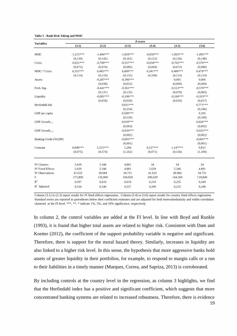
In column 1 of Table 5, the effects of the MSIC variable, the crisis dummy variable, and the
interaction between them on banking risk are tested. In line with what was indicated by
Gropp, Hakenes, and Schnabel (2011), we find that, in normal times, the MSIC coefficient is
significant and negative. Thus, an increase of 0.1 in the MSIC is associated with an average
decrease of 12.15% in the Z-score. Therefore, considering the reduction in the explained
variable, there is evidence that increases in the MSIC stimulate greater risk taking. The crisis
dummy is also linked to increases in bank risk, and it signals that, for a bank with a zero
MSIC, there is an average decrease of 47.8% (e-0.651
– 1) in the Z-score. Unlike the effect of
the MSIC variable when taken alone, its interaction with the crisis dummy has a positive and
significant impact on the risk level. Thus, although in periods of crisis the net effect of the
MSIC variable on the Z-score is still negative, there is an important reduction in its effect.
That is, in the banking turbulence phase, for an increase of 0.1 in the MSIC, there is an
average decrease of 8.64% in the Z-score. Thus, there is evidence corroborating hypothesis 1:
due to the governments’ limited ability to bailout financial institutions in times of crisis, an
increase in the MSIC may have a marginal effect that contributes to the decline in risk taking.
19
In column 2, the control variables are added at the FI level. In line with Boyd and Runkle
(1993), it is found that higher total assets are related to higher risk. Consistent with Dam and
Koetter (2012), the coefficient of the support probability variable is negative and significant.
Therefore, there is support for the moral hazard theory. Similarly, increases in liquidity are
also linked to a higher risk level. In this sense, the hypothesis that more aggressive banks hold
assets of greater liquidity in their portfolios, for example, to respond to margin calls or a run
to their liabilities in a timely manner (Marques, Correa, and Sapriza, 2013) is corroborated.
By including controls at the country level in the regression, as column 3 highlights, we find
that the Herfindahl index has a positive and significant coefficient, which suggests that more
concentrated banking systems are related to increased robustness. Therefore, there is evidence
Table 5 - Bank Risk Taking and MSIC
(3.1) (3.2) (3.3) (3.4) (3.5) (3.6)
MSIC -1,215*** -1,484*** -1,829*** -0,650*** -1,063*** -1,495***
(0,130) (0,142) (0,161) (0,122) (0,126) (0,148)
Crisis -0,651*** -0,700*** -0,557*** -0,658*** -0,702*** -0,570***
(0,072) (0,076) (0,085) (0,069) (0,072) (0,080)
MSIC * Crisis 0,351*** 0,485*** 0,409*** 0,341*** 0,480*** 0,479***
(0,114) (0,119) (0,132) (0,109) (0,114) (0,124)
Assets -0,287*** -0,396*** 0,005 0,006
(0,038) (0,052) (0,009) (0,009)
Prob. Sup. -0,441*** -0,361*** -0,512*** -0,570***
(0,137) (0,135) (0,078) (0,083)
Liquidity -0,081*** -0,106*** -0,160*** -0,163***
(0,018) (0,020) (0,016) (0,017)
Herfindahl Ind. 0,831*** 0,771***
(0,254) (0,246)
GDP per capita 0,599*** 0,105
(0,120) (0,100)
GDP Growth t-1 0,018*** 0,026***
(0,003) (0,002)
GDP Growth t-2 -0,030*** -0,032***
(0,002) (0,002)
Banking Credit (%GDP) -0,005*** -0,005***
(0,001) (0,001)
Constant 0,848*** 5,315*** 1,284 0,527*** 1,147*** 0,815
(0,075) (0,574) (1,162) (0,071) (0,156) (1,100)
Nº Clusters 5.639 5.346 4.881 34 34 34
Nº Fixed Effects 5.639 5.346 4.881 5.639 5.346 4.881
Nº Observations 41.632 38.084 34.731 41.632 38.084 34.731
F 275,800 126,960 104,920 296,630 144,560 118,840
R2
0,597 0,610 0,619 0,210 0,235 0,249
R2
Adjusted 0,534 0,546 0,557 0,209 0,235 0,248
Column (3.1) to (3.3) report results for FI fixed effects regressions. Column (3.4) to (3.6) report results for country fixed effects regressions
Standard errors are reported in parentheses below their coefficient estimates and are adjusted for both heteroskedasticity and within correlation
clustered at the FI level. ***, **, * indicate 1%, 5%, and 10% significance, respectively
VariablesZ-score

20
that is consistent with the charter value hypothesis. Similarly, increases in the GDP per capita
variable are also associated with lower risk taking.
With respect to the effects of economic growth on bank risk taking, it is observed that,
depending on the lag period, it is possible to have very different results. That is, when the
explanatory variable is used with a one-year lag, a 1% increase in economic growth is
reflected in lower risk taking, with an increase of 0.18% in the Z-score. By contrast, when a 2-
year lag is applied, the response is a decrease of 0.32% in the Z-score. Thus, there is evidence
pointing to the existence of the effect known in the literature as boom and bust (e.g., Hardy
and Pazarbasioglu, 1998; Schularick and Taylor, 2009).
More importantly, the addition of bank-level and country-level control variables to our
specification does not materially alter the coefficients of our variables of interest β1, β2 and β3.
The columns 4 to 6 of Table 5 report the regressions with country fixed effects instead of
bank fixed effects. Although the magnitude of β1 is slightly reduced as compared to the
counterpart regressions with bank fixed effects, our inferences remain the same.
5.2 Credit Default Swap Spread
In column 1 of Table 6, we test our second hypothesis that the country CDS spread is
associated with an increase in bank risk taking in normal times, but less so during financial
crises. The regression is estimated using bank fixed effects. First, we find that, in normal
times, the CDS coefficient is significant and negative. Thus, an increase of 100 bp in the CDS
is associated with an increase in risk taking, with an average decrease of 2.7% in the Z-score.
The negative and significant coefficient of the crisis dummy, in turn, indicates that times of
stress in the financial sector are linked to increases in risk taking. Finally, unlike the CDS
taken in isolation, there are signs that, in times of instability, an increase in the CDS reduces
risk taking. Thus, by raising the CDS spread by 100 bp, there is an average increase of 3.0%
in the Z-score. Therefore, there is evidence that a reduction in the country’s ability to pay its
debts is linked to a decrease in banking risk.

21
In column 2 of Table 6, we add the MSCI and its interaction with the crisis dummy. Not only
the inferences on the influence of the CDS spread are maintained (relative to column 1, Table
6), but also the coefficients of the added variables are very similar to the ones obtained in
Table 5. Finally, adding bank and other country-level control variables (column 3) and using
country fixed effects instead of bank fixed effects (columns 4 to 6) do not qualitatively alter
our inferences.
Table 6 - Bank Risk Taking, MSIC and CDS
Variables
(4.1) (4.2) (4.3) (4.4) (4.5) (4.6)
CDS -0,027*** -0,040*** -0,045*** -0,030*** -0,039*** -0,046***
(0,004) (0,004) (0,004) (0,004) (0,003) (0,004)
MSIC -1,586*** -2,288*** -1,145*** -1,929***
(0,133) (0,154) (0,122) (0,137)
Crisis -0,485*** -0,848*** -0,807*** -0,506*** -0,898*** -0,883***
(0,021) (0,083) (0,094) (0,020) (0,078) (0,089)
CDS*Crisis 0,057*** 0,085*** 0,124*** 0,071*** 0,086*** 0,142***
(0,015) (0,017) (0,021) (0,015) (0,016) (0,020)
MSIC*Crisis 0,591*** 0,668*** 0,651*** 0,818***
(0,133) (0,151) (0,126) (0,151)
Assets -0,422*** 0,008
(0,060) (0,010)
Prob. Sup. -0,337** -0,607**
(0,139) (0,087)
Liquidity -0,111*** -0,146***
(0,020) (0,017)
Herfindahl Ind. 0,851*** 0,596**
(0,296) (0,296)
GDP per capita 0,827*** 0,323***
(0,135) (0,114)
GDP Growth t-1 0,016*** 0,023***
(0,003) (0,002)
GDP Growth t-2 -0,034*** -0,037***
(0,002) (0,002)
Banking Credit (%GDP) -0,002 -0,001
(0,001) (0,001)
Constant 0,183*** 1,094*** -0,822 0,188*** 0,846*** -1,776
(0,006) (0,076) (1,354) (0,015) (0,071) (1,263)
Nº Clusters 5424 5424 4758 5424 5424 4758
Nº Fixed Effects 5424 5424 4758 32 32 31
Nº Observations 37.670 37.670 32.061 37.670 37.670 32.061
F 243,69 184,07 94,520 286,83 194,65 105,410
R2
0,603 0,607 0,627 0,212 0,215 0,251
R2
Adjusted 0,536 0,541 0,561 0,211 0,214 0,250
Column (4.1) to (4.3) report results for FI fixed effects regressions. Column (4.4) to (4.6) report results for country fixed effects
regressions. Standard errors are reported in parentheses below their coefficient estimates and are adjusted for both heteroskedasticity
and within correlation clustered at the FI level. ***, **, * indicate 1%, 5%, and 10% significance, respectively
Z-Score

22
The results shown in Table 7 have the triple interaction between CDS, MSIC, and Crisis as its
main variable of interest. In the specification with country fixed effects, in column 2, the
triple interaction is positive and significant at the 10% level. In this line, with a fixed MSIC
index, we find that, in periods of crisis, increases in the CDS are associated with lower risk
taking, or, similarly, with a fixed CDS spread, increases in the MSIC are associated with
lower bank risk taking during crises.
However, when we use bank fixed effects, the coefficient of the triple interaction is positive,
but not statistically significant. It is indeed possible that the bank fixed effects capture most of
the cross sectional variation in MSIC, which makes the remaining time-variation too small to
Table 7 - Bank Risk Taking and Triple Interaction
(5.1) (5.2)
CDS -0,056*** -0,052***
(0,004) (0,004)
MSIC -1,641*** -1,197***
(0,133) (0,123)
Crisis -0,814*** -0,801***
(0,101) (0,091)
CDS*MSIC 0,121*** 0,100***
(0,021) (0,020)
CDS*Crisis 0,024 -0,028
(0,070) (0,047)
MSIC*Crisis 0,564*** 0,506***
(0,163) (0,150)
CDS*MSIC*Crisis 0,042 0,149*
(0,110) (0,079)
Constant 1,094*** 0,850***
(0,076) (0,071)
Nº Clusters 5424 5424
Nº Fixed Effects 5424 32
Nº Observations 37.670 37.670
F 129,470 140,320
R2
0,608 0,215
R2
Adjusted 0,542 0,215
Column (5.1) reports results for FI fixed effects regressions. Column (5.2) reports results
for country fixed effects regressions. Standard errors are reported in parentheses below their
coefficient estimates and are adjusted for both heteroskedasticity and within correlation
clustered at the FI level. ***, **, * indicate 1%, 5%, and 10% significance, respectively
Z-Score Z-ScoreVariables

23
be “spread” among three variables (MSIC, its interaction with Crisis and the triple
interaction). In addition, most of our previous inferences are maintained.
5.3 Robustness Tests
We follow Beck, De Jonghe, and Schepens (2013) and separately analyze the effects of our
independent variables in the 3 components of the z-score: ROA, Capital to Assets ratio, and
the standard deviation of ROA. The results are shown in Table 8.
Table 8 - Bank Risk Taking and Z-Score Components
Variables
(6.1) (6.2) (6.3) (6.4) (6.5) (6.6)
CDS -0,095*** -0,079*** -0,012*** -0,011*** 0,039*** 0,040***
(0,025) (0,021) (0,003) (0,003) (0,003) (0,003)
Crisis -0,243*** -0,313*** -0,141*** -0,226*** 0,636*** 0,629***
(0,060) (0,062) (0,021) (0,027) (0,089) (0,084)
CDS*Crisis 0,108*** 0,098*** 0,011 0,014* -0,107*** -0,119***
(0,018) (0,018) (0,007) (0,007) (0,017) (0,016)
Assets -0,224*** -0,070*** -0,283*** -0,098*** 0,144** -0,099**
(0,040) (0,007) (0,022) (0,005) (0,058) (0,010)
Prob. Sup. -0,096 0,268*** -0,000 -0,104** 0,343*** 0,699***
(0,068) (0,064) (0,033) (0,046) (0,127) (0,081)
Liquidity -0,018 -0,020 -0,021*** -0,009 0,090*** 0,156***
(0,012) (0,014) (0,005) (0,010) (0,019) (0,020)
Herfindahl Ind. 1,215*** 1,161*** 0,093 0,304 -0,617** -0,156
(0,234) (0,264) (0,104) (0,101) (0,263) (0,268)
GDP per capita -0,313*** -0,451*** 0,776*** 0,551*** -0,118 0,165
(0,098) (0,073) (0,037) (0,028) (0,128) (0,111)
GDP Growth t-1 0,001 0,004** -0,009*** -0,007*** -0,026*** -0,030***
(0,001) (0,001) (0,000) (0,000) (0,002) (0,002)
GDP Growth t-2 -0,001 -0,001 0,005*** 0,004*** 0,041*** 0,043***
(0,002) (0,002) (0,000) (0,000) (0,002) (0,002)
Banking Credit (%GDP) -0,004*** -0,006*** -0,004*** -0,005*** -0,002* -0,004*
(0,001) (0,001) (0,000) (0,000) (0,001) (0,001)
MSIC -0,277*** -0,420*** -0,149*** -0,181*** 2,104*** 1,706***
(0,074) (0,074) (0,034) (0,039) (0,143) (0,132)
MSIC*Crisis 0,183* 0,345* 0,096*** 0,255*** -0,537*** -0,531***
(0,102) (0,106) (0,036) (0,047) (0,141) (0,134)
Constant 6,041*** 5,505*** -1,612*** -1,888*** -4,697*** -4,095***
(0,975) (0,846) (0,322) (0,340) (1,276) (1,195)
Nº Clusters 4673 4673 4758 4758 4758 4758
Nº Fixed Effects 4673 31 4758 31 4758 31
Nº Observations 29.200 29.200 32.061 32.061 32.061 32.061
F 46,190 40,370 136,270 136,270 90,460 109,350
R2
0,730 0,264 0,921 0,290 0,674 0,315
R2
Adjusted 0,679 0,263 0,908 0,289 0,617 0,314
Column (6.1) , (6.3) and (6.5) report results for FI fixed effects regressions. Column (6.2) , (6.4) and (6.6) report results for country fixed effects
regressions. Standard errors are reported in parentheses below their coefficient estimates and are adjusted for both heteroskedasticity and within
correlation clustered at the FI level. ***, **, * indicate 1%, 5%, and 10% significance, respectively
Capital to Assets Ratio Standard Deviation of ROAROA

24
The coefficients of the variables MSIC, CDS, and the interaction of both with the crisis
dummy have an expected sign and a significant relationship with the 3 regressands. More
specifically, in column 1 of Table 8, the results show that the ROA is 24.3 percentage points
(pp) smaller during the crisis (results statistically significant at 1%) for a bank located in a
country with a CDS spread and MSIC equal to zero. An increase of 100 bps in the CDS
spread is associated to an average decrease of 9.5 pp in the ROA in normal times. In turn, this
relationship is considerably changed in times of crisis. That is, every increase of 100 bp in the
CDS represents an increase of 1.30 pp (100 * (-0.095 + 0.108)) in the ROA.
Concerning the MSIC, there is an alignment with Gropp, Hakenes, and Schnabel (2011),
which suggests that increases in this variable are related to decreases in profitability. For each
increment of 0.1 in the MSIC, the ROA is reduced by 2.77 pp (-0.277 * 0.1). However, the
MSIC negative effect on profitability is substantially mitigated during the crisis. In this case,
for increases of 0.1 in the MSIC, a reduction of only 0.94 pp is observed ((-0.183 + 0.277) *
0.1) in the profitability indicator.
The negative and significant coefficient of the Assets variable points to a decrease in
profitability, whereas the total assets increase. Thus, an increase of 1% in the balance of assets
of the FI corresponds to a decrease of 0.224 pp in the ROA. By reexamining the coefficient of
the Herfindahl variable, the charter value hypothesis is confirmed. That is, it is found that
increases of 10 bp in the concentration index result in increases of 12.15 pp in the ROA.
The coefficient of the GDP per capita variable, which is negative and significant, provides
evidence that the average profitability of FIs operating in developed countries is lower than
that of FIs operating in developing countries. Along these lines, it is found that, for each 1%
increase in the GDP per capita, the ROA is reduced by 0.313 pp.
In column 3 of Table 8, we run an analogous regression using the Capital to Assets Ratio as
the dependent variable. In line with what was indicated above, increases in the CDS spread
rate are related to decreases in the dependent variable, i.e., greater risk taking. However, there
is an inversion in the sign of the coefficient in periods of crisis. Thus, while in normal times,
an increase of 100 bps in the CDS corresponds to a 1.2 pp decrease (100 * -0.012 * 1) in the
index, during crises, the same variation is linked to an increase of 0.8 pp (100 * (-0.012 +
0.020) * 1) in the ratio.

25
Regarding the impact of the MSIC on the Capital to Assets ratio, the hypothesis that, in
normal times, increases in this variable are related to greater risk taking, is again corroborated.
Thus, for each increase of 10 bps in the MSIC, the Capital to Assets ratio is reduced by 1.49
pp (100 * -0.149 * 0.1). However, during the crisis, the negative effect of the MSIC on
profitability is substantially mitigated: a 10 bp increase in the MSIC is associated to a
reduction in the indicator of only 0.53 pp (100 * (-0.149 + 0.096) * 0.1).
Finally, in Table 9 it is confirmed that FIs located in countries with high CDS spreads are less
risky than FIs located in countries with low CDS spreads in normal times. During the crisis
however, banks in high-CDS countries increase their risk more than banks in low CDS
countries. This result suggests that, during the crisis, FIs acting in countries with smaller
bailout capacity (high CDS) increase their risk taking less than their counterparties in the low
credit risk countries, possibly because they are less likely to be bailed out.
Table 9 - Difference - in - Differences Model
LCDS 0,840*** -0,690*** -0,310*** -1,155***
(0,021) (0,014) (0,008) (0,022)
Crisis -0,256*** -0,199*** 0,033** 0,281***
(0,035) (0,024) (0,014) (0,036)
LCDS * Crisis -0,098** 0,212*** 0,012 0,115***
(0,040) (0,027) (0,016) (0,042)
Constant -0,519*** -0,534*** 2,226*** -1,814***
(0,018) (0,012) (0,007) (0,019)
Nº observations 41.632 38.002 41632 41632
F 782,320 878,630 596,460 128,590
R2
0,050 0,060 0,041 0,085
Standard errors are reported in parentheses below their coefficient estimates are adjusted for both
heteroskedasticity and within correlation clustered at the FI level. ***, **, * indicate 1%, 5%, and 10%
significance, respectively.
Variables Z-score ROACapital to Assets
Ratio
Standard Deviation
of ROA

26
6 Conclusion
The goal of this article is to assess the impact of government rescue expectation on bank risk
in periods of crisis and normality. Additionally, it is tested whether the countries’ financial
capacity, measured by the Credit Default Swap (CDS) spread, can contribute to changing this
effect.
In line with the moral hazard hypothesis, it is found that increases in the bailout expectation
and the total assets of an institution are associated with greater risk taking. In addition, the
market share of insured competitors (MSIC) or the rescue expectation of the competitors of an
institution also influences its risk taking. However, depending on the period of analysis, this
link can be different; that is, in normal periods, there is a predominance of the channel
through which increases in the MSIC distort competition, reduce profit margins, and increase
the risk taking of small institutions. During crises, however, increases in the MSIC indicate
lower risk taking. It is assumed that the reason is, the higher the MSIC of an institution, the
lower its relative importance in the system and thus the lower its prospect of eventually being
rescued. Therefore, there is greater conservatism.
Similarly, we observe that the association between sovereign CDS spread and banking risk is
modified during the crisis. Thus, while in normal times, increases in the sovereign CDS are
linked to higher levels of banking risk, in the crisis, this effect is reversed. That is, in line with
the moral hazard hypothesis, by raising the CDS and thus reducing the financial ability of a
country to undertake bank bailouts during the crisis, there is a decrease in the appetite for risk.
Finally, corroborating previous results, indications are found that, during the crisis,
institutions located in countries with high CDS spreads have, on average, an increase in the
risk level that is lower than that in countries with low CDS spreads.

27
7 References
ACHARYA, V. V., ANGINER, D., WARBURTON, A. J. (2013). The end of market
discipline? Investor expectations of implicit state guarantees. December).www.papers.ssrn.
com/sol3/papers.cfm
ACHARYA, V., DRECHSLER, I., SCHNABL, P. (2014). A pyrrhic victory? Bank bailouts
and sovereign credit risk. The Journal of Finance, 69(6), 2689-2739.
ANGINER, D., DEMIRGÜÇ-KUNT, A., ZHU, M. (2014). How does deposit insurance affect
bank risk? Evidence from the recent crisis. Journal of Banking & finance, 48, 312-321.
ANGKINAND, A., WIHLBORG, C. (2010). Deposit Insurance coverage, ownership, and
banks’ risk-taking in emerging markets. Journal of International Money and Finance, 29(2),
252-274.
BECK, T., DE JONGHE, O., SCHEPENS, G. (2013). Bank competition and stability: cross-
country heterogeneity. Journal of financial Intermediation,22(2), 218-244.
BERGER, A. N., KLAPPER, L. F., ARISS, R. T. (2009). Bank competition and financial
stability, Journal of Financial Services Research, April 2009, Volume 35, Issue 2, pp 99-118
BOYD, J. H., RUNKLE, D. E. (1993). Size and performance of banking firms: Testing the
predictions of theory. Journal of monetary economics, 31(1), 47-67.
BREWER, E., JAGTIANI, J. (2013). How much did banks pay to become too-big-to-fail and
to become systemically important?. Journal of Financial Services Research February 2013,
Volume 43, Issue 1, pp 1-35.
BROECKER, T. (1990). Credit-worthiness tests and interbank competition. Econometrica,
Vol. 58, No. 2, 429-452.

28
CAMERON, A. C., MILLER, D. L. (2015). A practitioner’s guide to cluster-robust
inference. Journal of Human Resources, 50(2), 317-372.
CANTOR, R., PACKER, F. (1996). Determinants and impact of sovereign credit
ratings. Economic policy review, 2(2).
CORREA, R., LEE, K., SAPRIZA, H. SUAREZ, G. (2014). Sovereign credit risk, banks’
government support, and bank stock returns around the world. Journal of Money, Credit and
Banking, 46(s1), 93-121.
DAM, L., KOETTER, M. (2012). Bank bailouts and moral hazard: empirical evidence from
Germany. Review of Financial Studies, 25(8), 2343-2380.
DAMAR, E. GROPP, R. MORDEL, A. (2012). The Ex-Ante Versus Ex-Post Effect of Public
Guarantees. Bank of Canada Working Paper.
DEMIRGÜÇ-KUNT, A. (1998) Designing a Bank Safety Net – A long Term Perspective –
http://www1.worldbank.org/finance/html/designing_a_bank_sn.html
DEMIRGÜÇ-KUNT, A., DETRAGIACHE, E. (1998). The determinants of banking crises in
developed and developing countries. Staff Papers-International Monetary Fund, 81-109.
DEMIRGÜÇ-KUNT, A., & DETRAGIACHE, E. (2005). Cross-country empirical studies of
systemic bank distress: a survey. National Institute Economic Review,192(1), 68-83.
DEMIRGÜÇ-KUNT, A., DETRAGIACHE, E., MERROUCHE, O. (2013). Bank Capital:
Lessons from the Financial Crisis. Journal of Money, Credit and Banking, 45(6), 1147-1164.
DEMIRGÜÇ-KUNT, A., HUIZINGA, H. (2013). Are banks too big to fail or too big to
save? International evidence from equity prices and CDS spreads. Journal of Banking &
Finance, 37(3), 875-894.
DEMIRGÜÇ-KUNT, A., KANE, E. LAEVEN, L. (2008). Determinants of deposit-insurance
adoption and design. Journal of Financial Intermediation, 17(3), 407-438.

29
DEMIRGÜÇ-KUNT, KARACAOVALI, B., LAEVEN, L. (2005). Deposit Insurance around
the world: a comprehensive database. World Bank Policy Research Working Paper, (3628).
DUCHIN, R., SOSYURA, D. (2014). Safer ratios, riskier portfolios: Banks׳ response to
government aid. Journal of Financial Economics, 113(1), 1-28.
DUTTAGUPTA, R., CASHIN, P. (2011). Anatomy of banking crises in developing and
emerging market countries. Journal of International Money and Finance, 30, 354–376.
FLANNERY, M. J. (1998). Using market information in prudential bank supervision: A
review of the US empirical evidence. Journal of Money, Credit and Banking, 273-305.
GROPP, R., HAKENES, H., SCHNABEL, I. (2011). Competition, risk-shifting, and public
bail-out policies. Review of Financial Studies, 24(6), 2084-2120.
HAKENES, H., SCHNABEL, I. (2010). Banks without parachutes: Competitive effects of
government bail-out policies. Journal of Financial Stability, 6, 156–168.
KANE, E. (2000a). Designing financial safety nets to fit country circumstances. World Bank
policy research working paper, (2453).
KEELEY, M., (1990). Association Deposit Insurance, Risk, and Market Power in Banking.
The American Economic Review, Vol. 80, No. 5, pp. 1183-1200
LAEVEN, L., VALENCIA, F. (2012). Systemic banking crises database: an update
MARQUES, L. B., CORREA, R., SAPRIZA, H. (2013). International evidence on
government support and risk taking in the banking sector. FRB International Finance
Discussion Papers, (1086).
MOOSA I. A. (2010). The Myth of Too Big to Fail. London: Palgrave MacMillan
OLIVEIRA, R. F., SCHIOZER, R. F., BARROS, L. A. B. C. (2015). Depositors’ Perception
of “Too-Big-to-Fail”. Review of Finance, 19(1), 191–227.
PISCHKE, J. S., ANGRIST, J. D. (2009). Mostly Harmless Econometrics.

30
SAPIENZA, P. (2004). The effects of government ownership on bank lending. Journal of
Financial Economics, 72, 357–384.
SCHICH, S., LINDH, S. (2012). Implicit guarantees for bank debt. OECD Journal: Financial
Market Trends, 2012(1), 45-63.
SOEDARMONO, W., MACHROUHB, F., TARAZI, A. (2013). Bank competition, crisis
and risk taking: Evidence from emerging markets in Asia. Journal of Int. Fin. Markets, Inst.
and Money, 23, 196– 221.