Baha Alzalg, Catalina Anghel, Wenying Gan, Qing Huang ... · BAHA ALZALG, CATALINA ANGHEL, WENYING GAN, QING HUANG, MUSTAZEE RAHMAN, AND ALEX SHUM Abstract. The optimal power ow problem

A COMPUTATIONAL ANALYSIS OF THE OPTIMAL POWER FLOW PROBLEM

By

Baha Alzalg, Catalina Anghel, Wenying Gan, Qing Huang, Mustazee Rahman, Alex Shum

IMA Preprint Series #2396

(May 2012)

INSTITUTE FOR MATHEMATICS AND ITS APPLICATIONS

UNIVERSITY OF MINNESOTA

400 Lind Hall

207 Church Street S.E.

Minneapolis, Minnesota 55455-0436

Phone: 612-624-6066 Fax: 612-626-7370

URL: http://www.ima.umn.edu

A COMPUTATIONAL ANALYSIS OF THE OPTIMAL POWER FLOW

PROBLEM

BAHA ALZALG, CATALINA ANGHEL, WENYING GAN, QING HUANG, MUSTAZEE RAHMAN,AND ALEX SHUM

Abstract. The optimal power flow problem is concerned with finding a proper operating pointfor a power network while attempting to minimize some cost function and satisfy several networkconstraints. In this report we analyze the optimal power flow problem subject to contingencyconstraints, which demands that there be enough power to meet demands in the network in theevent of contingencies such as a fault in some transmission line or the loss of a generator. We developnumerical algorithms to handle this problem for the e− 1 security constrained optimal power flowproblem. We also investigate the relationship between the cost of the optimal power flow problemand network topology. We find that when the network topology is that of a small world graph or ascale-free graph, the optimal power flow problem is quite robust in terms of satisfying contingencyconstraints.

Contents

1. Introduction 1Acknowledgements 22. Background 22.1. The power flow equations 22.2. The optimal power flow problem 32.3. The MATPOWER package 42.4. Graph theoretic notions 43. Security constrained optimal power flow 53.1. The single e− 1 security-constrained OPF 63.2. The full e− 1 security-constrained OPF 74. Effects of network topology 94.1. SCOPF for cycle, bipartite, and complete graphs 94.2. OPF on small world graphs 114.3. OPF on scale free graphs 154.4. Comparison of costs of SCOPF for various graphs 18References 19

1. Introduction

Modern electrical networks are complex structures whose effective operation is vital towardstasks as minute as everyday chores to large scale industrial activities. As such it is necessary todesign these networks so that they can meet demands even under various contingencies, such asthe breakdown of a generator or a fault in some transmission line. The importance of being ableto supply power under these contingencies was exemplified by the blackout in the North Americanpower grid during 2003, the largest ever experienced in North America, that affected about 50million people in parts of Ohio, Michigan, New York, Pennsylvania, New Jersey, Connecticut,

1

2 B. ALZALG, C. ANGHEL, W. GAN, Q. HUANG, M. RAHMAN, AND A. SHUM

Massachusetts, Vermont, as well as Ontario and Quebec for 2 to 7 days. The reason for theblackout was a failure of only a handful of contingencies in the network [8].

In this article we address the issue of efficient transmission of power in power networks undersuch contingency constraints. We also focus on the effect of the network topology on the efficienttransmission of power. The mathematical model for the transmission of power through a network,given by the power flow equations, is well understood. In Sections 2 we introduce the power flowequations along with the related optimal power flow problem that deals with transmission of powerthrough a network under the objective of minimizing a cost function.

In Section 3 we deal with the optimal power flow problem under certain contingency constraintsand demonstrate the effect of contingencies on the minimal cost. To this end we develop an algo-rithm that can compute the minimal cost for the optimal power flow problem under contingenciesgiven the network data.

Section 4 is devoted to the study of the relationship between a power network’s topology andthe optimal power flow problem (with and without contingencies). We explore how the minimalcost of the optimal power flow problem varies depending on certain network parameters such as itsaverage degree, average path length and algebraic connectivity.

Acknowledgements

This work was conducted at the IMA while the authors were participating in the workshop‘Mathematical Modeling in Industry XV’. The authors are grateful to Chai Wah Wu, the team’smentor, for his guidance throughout the project and for his insights into the problem. The authorswould also like to thank the IMA and the organizers of the workshop for their hospitality.

2. Background

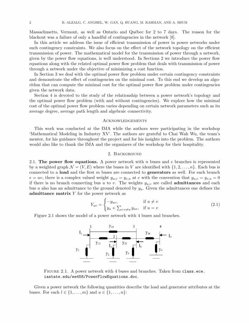
2.1. The power flow equations. A power network with n buses and e branches is representedby a weighted graph N = (V,E) where the buses in V are identified with {1, 2, . . . , n}. Each bus isconnected to a load and the first m buses are connected to generators as well. For each branche = uv, there is a complex valued weight yu,v = yv,u at e with the convention that yu,v = yv,u = 0if there is no branch connecting bus u to v. The weights yu,v are called admittances and eachbus u also has an admittance to the ground denoted by yu. Given the admittances one defines theadmittance matrix Y for the power network as

Yuv =

{−yuv, if u 6= v

yu +∑

v:v 6=u yuv, if u = v(2.1)

Figure 2.1 shows the model of a power network with 4 buses and branches.

Figure 2.1. A power network with 4 buses and branches. Taken from class.ece.

iastate.edu/ee458/PowerFlowEquations.doc.

Given a power network the following quantities describe the load and generator attributes at thebuses. For each l ∈ {1, . . . ,m} and u ∈ {1, . . . , n}:

class.ece.iastate.edu/ee458/PowerFlowEquations.doc

class.ece.iastate.edu/ee458/PowerFlowEquations.doc

OPTIMAL POWER FLOW 3

• P du and Qdu are the real and reactive power demands at bus u respectively. These are givendemands that must be met in order to have a proper power supply throughout the network.• P gl and Qgl are the real and reactive powers generated at bus l respectively. These are

variables.

The voltage at bus u is denoted by Vu ∈ C, and V = [V1, . . . , Vn]T is the column vector consistingof all the voltages. Similarly, the current injection at bus u is denoted by Iu and I = [I1, . . . , In]T

represent the vector of all currents in the network. The relation governing the currents and voltagesis

I = Y V . (2.2)

One defines the net power injection at bus u to be Su = VuI∗u where ∗ denotes complex

conjugation. Throughout this report i =√−1 denotes the imaginary unit. The power flow

equations for the network state that

(P gl − Pdl ) + i(Qgl −Q

dl ) = VlI

∗l for1 ≤ l ≤ m (2.3)

−P du − iQdu = VuI∗u form+ 1 ≤ u ≤ n . (2.4)

The power flow equation (2.3) are often written using real variables. To this end write Vu =|Vu|eiθu = |Vu|(cos(θu) + i sin(θu)), Y = G + iB, and adopt the convention that P gu = 0 if u > m.Simplifying (2.3) gives

(P gu − P du ) + i(Qgu −Qdu) = Vu(n∑

w=1

YuwVw)∗

= |Vu|eiθun∑

w=1

(Guw − iBuw)(|Vw|e−iθw)

=

n∑w=1

|Vu||Vw|ei(θu−θw) (Guw − iBuw)

=n∑

w=1

|Vu||Vw| (cos(θu − θw) + i sin(θu − θw)) (Guw − iBuw).

Separating the equations into its real and imaginary parts one obtains

P gu − P du =

n∑w=1

|Vu||Vw| (Guw cos(θu − θw) +Buw sin(θu − θw)) (2.5)

Qgu −Qdu =

n∑w=1

|Vu||Vw| (Guw sin(θu − θw)−Buw cos(θu − θw)) . (2.6)

In equations (2.5) and (2.6) there are 4 sets of variables, P gl , Qgl for i ≤ l ≤ m and |Vu|, θu for

1 ≤ u ≤ n. The goal is to solve these non-linear equations in the given variables. The approachfor solving the power flow equations is to use an iterative algorithm. In commercial programs theNewton-Raphson algorithm is commonly used.

2.2. The optimal power flow problem. The objective in the optimal power flow (OPF) prob-lem is to find an optimal operating point of the network that minimizes an appropriate cost subjectto certain constraints on loads, powers, voltages variables and branch flows. The cost may be, forexample, generation cost or transmission loss. The OPF problem has been extensively studied inliterature beginning with the work of Carpentier [2] in 1962. Several algorithms have been devel-oped to tackle this highly non-linear problem including Newton-Raphson, quadratic programming,


non-linear programming, LP relaxations and various interior point methods (see [4, 5, 6] and thereferences cited therein). The OPF problem is in general NP-hard [7].

The classical OPF problem is formulated as

minV, Pg , Qg

∑ml=1 fl(P

gl ) subject to

SlI∗l = (P gl − P

dl ) + i(Qgl −Q

dl ) for 1 ≤ l ≤ m

SuI∗u = −P du − iQdu for m+ 1 ≤ u ≤ n

Pminl ≤ P gl ≤ Pmaxl for 1 ≤ l ≤ m

Qminl ≤ Qgl ≤ Qmaxl for 1 ≤ l ≤ m

V minu ≤ |Vu| ≤ V max

l for 1 ≤ u ≤ nθminu ≤ θu ≤ θmaxu for 1 ≤ u ≤ n

Other constraints are possible as well. For example, we could impose bounds on the voltageangle differences: |θu − θw| ≤ θmax for all 1 ≤ u,w ≤ n. The cost functions fl(P

gl ) are typically

taken to be polynomials (often quadratic polynomials).

2.3. The MATPOWER package. The research and modeling of the power flow and OPF prob-lems were done entirely using the MATPOWER toolbox version 4.0 in MATLAB [10]. The MAT-POWER toolbox was created by Zimmerman and Sanchez to numerically handle the power flowequations and the OPF problem among other things. A detailed manual is available on their web-site at http://www.pserc.cornell.edu/matpower/. The toolbox is capable of modeling complexnetworks, providing properties of buses, branches, generators, generator costs and loads. Thesequantities are all given in matrices that can be easily modified. The power flow cost problem issolved using the Newton-Raphson method, while the OPF problem has several different solvers.The solver is set to the default MATLAB Interior-Point Solver (MIPS), and was used to solveall the OPF problems. The majority of the produced code focused on building the correspondingmatrices in our problems for MATPOWER to solve.

A variety of different case files were provided with the toolbox that are representative of realnetworks. Several of them were tested and their results are shown in this report report. Theformat is simple enough to build our own examples. The following functions were used extensivelyto obtain the data shown throughout this report.

r = runpf(casefile,options)

The function runpf solves the power flow equation (2.3) given the values of P gl and Qgl for thevariables Vu = (|Vu|, θu). The input casefile takes in a structure with the necessary matricesfor buses, generators and branches. The output r is a structure that includes the values for thevariable Vu. The options input controls various parameters. The reader is encouraged to refer tothe MATPOWER manual to see its descriptions.

r = runopf(casefile,options)

The function runopf solves the OPF problem. The inputs and outputs are the same format asrunpf. Instead, the Pg and Qg values are unknown, and a minimization is performed accordingto the given cost function. The output of interest in the structure r, are the cost, as well as theoptimal supplies for each generator.

2.4. Graph theoretic notions. In the report, we try to correlate the ratio of the OPF cost of anetwork to a subnetwork obtained by removing one branch with several topological properties ofthe network. We also try to do the same for the OPF cost with contingency constraints. Hence inthis section, we will introduce several graph theoretic definitions that we will use later.

Let G = (V,E) be a simple graph. The first notion is that of algebraic connectivity of G.The algebraic connectivity reflects how well connected the overall graph is, and has been used in

http://www.pserc.cornell.edu/matpower/


analyzing the synchronizability of networks. Meanwhile, we suspect that power generation cost ishighly related to the connectedness of the underlying network topology. For this reason we discussthe algebraic connectivity. For a simple graph G, the graph Laplacian LG is defined as:

LG(u, v) =

−1, if u is adjacent to vand u is not the same as v

deg(v), if u = v

0, otherwise

The algebraic connectivity is defined as the second smallest eigenvalue of LG. The algebraicconnectivity of G is greater than 0 if and only if G is connected. Usually the bigger the algebraicconnectivity the better the graph is connected.

The second definition we need is the average path length of G. For each pair of vertices u, vin G, the distance between them, denoted d(u, v), is the length of the shortest path connecting uand v. If u and v are not connected, the distance is infinite. The average path length l(G) is theaverage distance for all possible pairs of different vertices in G. It is a measure of the efficiency ofinformation or mass transport on a network. If n is the number of vertices in G, then

lG =

∑u,v∈V d(u, v)

n(n− 1).

The third notion is the average vertex degree. The degree of a vertex v in G is the number ofedges it is connected with, we can write it as deg(v). The average degree is the average degree overall vertices:

AvDG =

∑v∈V deg(v)

n=

2e

n.

Here e is the number of edges in G and n is the number of vertices.

3. Security constrained optimal power flow

In the report thus far, the power flow equations and the OPF problem have been presented. Wenow consider the OPF under contingency constraints as advertised. Suppose we are given a powernetwork as described in Section 2.1; let n and e denote the number of buses and branches in thenetwork respectively. It is of interest to investigate the effects of cutting a branch from the network.When branches are cut, internal power values in the branches and buses change, potentially causingpower failures or generator and load disconnections. Generators may have to change their powersupplies, and startup and shutdown costs can be expensive. There are several new problems thatarise.

(1) Can power still be supplied to the loads in the new network? If so, what are the optimalpower generations?

(2) Suppose we are interested in a specific branch being cut. Can the optimal power flowproblem be solved simultaneously for both the original network and the new network?That is, we wish to find power supply values that can satisfy both the original and thesub-network resulting from one of the branches being cut. Is this even feasible?

(3) A tougher problem: what if we want uninterrupted power supply in both networks nomatter which branch is being cut (i.e. one can remove exactly one branch but is it notknown which one in advance).

Limiting factors would include the exclusion of generators and limits in the power transferablethrough the branches. The first problem is simply solving the optimal power flow problem in thecontext of a new network. A solution to the branch cutting problem (the first problem above) doesnot necessarily yield a feasible point in the original OPF problem. Simply raising the generatorvalues might not satisfy the constraints for both problems. The power flow equations are highlynonlinear and the internal properties of the network must be considered. The second and third


problems are more difficult. Our goal is to prevent a power failure should a branch be cut. It mayseem wasteful to provide unnecessary power that is not used. In the setting of large scale electricalgrids however, additional power should be supplied since the load demands constantly change. Ourefforts have been focused on the second and third problems. To reiterate, the second problem isnot the optimal power flow with a branch cut from the original network. The last two problemsare known in literature as the e− 1 security-constrained optimal power flow (SCOPF) problem.

3.1. The single e−1 security-constrained OPF. Recall the optimal power flow problem givenin Section 2.2. Since we are dealing with two problems simultaneously, it is necessary to constructa new set of variables x′ = [P g

′, Qg

′, V ′]T that corresponds to the new problem on the sub-network

resulting from a branch being removed. Next, we require that this new set of variables x′ tosatisfy its own corresponding power flow equations for the sub-network. Finally, we would like thecorresponding powers in the generators to be the same (resulting in uninterrupted power flow).Since they are the same, it is not necessary to change the cost function from the original problem.To summarize, the SCOPF problem has the following additional constraints:

g1(x′) = 0

h1(x′) ≤ 0, and

P g′

l = P gl .

Here g1 represents the power flow equation 2.3 for the new sub-network, and h1 represent theinequality constraints for the OPF problem on said sub-network.

In terms of implementation in MATPOWER, we perform the following adjustments to the orig-inal case file.

(1) Bus matrix: We add one duplication to the original bus matrix but remark the bus numberfrom n+ 1 to 2n in the duplication island.

(2) Generator matrix: Add one duplication to the original generator matrix.(3) Branch matrix: Add one duplication to the original branch matrix, change the bus number

accordingly, and delete the branch row we want to cut.(4) Generator cost matrix: No change.

One more thing to mention is that MATPOWER usually picks the first generator bus as thereference bus. When we make duplication, we keep the reference bus type in the duplicated part.The two islands are actually regarded as unconnected, we set a reference bus in each island whichhelps convergence.

Our goal is to identify which branch is the most problematic, which requires checking each e− 1contingency case and the resulting cost. The largest optimal cost shows that the correspondingbranch is the most problematic. We would like to illustrate this through two examples.

Example 3.1. 9-bus case. The 9-bus case comes from MATPOWER. The network is shown inFigure 2. There are three generator buses and three nonzero load buses. Table 1 shows thatthe original uncut model has the lowest optimal cost. This is trivial because when we considercontingencies regarding the removal of a branch, we add constraints to the original OPF problem.The feasible region decreases, which leads to the increase of optimal cost value. Among thesecontingencies, we see that the removal of branches (1, 4), (3, 6), and (8, 2) leads to relatively higheroptimal costs. These branches are all connected to generator buses which become isolated afterthe corresponding branches are removed. Understandably, the isolation (i.e. loss) of a generator isexpensive for a network, and so the removal of branches that do so are relatively more problematic.We also observe that the contingency corresponding to branch (8, 2) being cut has the largestoptimal cost (the most problematic branch cut). This indicates that the generator attached to


Branch Cut Optimal Cost

No cuts 5296.7

(1, 4) 6682.6

(4, 5) 5331.2

(5, 6) 5885.4

(3, 6) 6846.3

(6, 7) 5330.7

(7, 8) 5525.9

(8, 2) 7935.4

(8, 9) 5576.8

(9, 4) 5587.4

Table 1. Numerical re-sults for 9-bus case.

Table 2. Graph for 9-bus case.

bus 2 is most vital to this power network, and its removal incurs the most cost for meeting powerdemands.

Example 3.2. 14-bus case. The 14-bus case also comes from MATPOWER. The original networkgraph is shown in Figure 4. From the results in Table 3, we find that the removal of branches (1, 5),(2, 4), and (4, 5) make the numerical solver for the SCOPF problem not converge (more precisely,the constraints added to satisfy the contingencies leads the MATPOWER solver to not converge).One possible reason is that there is no feasible solution satisfying all the constraints. For instance,the contingency of branch (1, 5) being cut could make the network fail. The load demands cannot be met simultaneously with the power flow constraints when this branch is cut. From theOPF solution of original non-contingency case, we have Pg,1 = 194.33, Pg,2 = 36.72, Pg,3 = 28.74,Pg,6 = 0, and Pg,8 = 8.5. The power generation at bus 1 is the largest, which would explain whybranch (1, 2) being removed could lead to a higher cost.

3.2. The full e− 1 security-constrained OPF. In the previous part, we discuss the case withe− 1 contingencies of cutting a branch. Now we extend the idea to e− 1 contingencies of cuttingany one branch, which is problem (3) mentioned at the beginning of this section. In reality, fora complex power network, it is possible that one of the branches may fail while we still need thepower flow work properly.

The scheme of this problem is similar as the previous SCOPF model. But we extend to make eduplications since we want the system satisfying all e−1 contingencies. In terms of implementationof MATPOWER, the adjustment is shown as follows:

(1) Bus matrix: We add e duplications to the original bus matrix but remark the bus numberstarting from n+ 1 to n(e+ 1) for these duplicated islands.

(2) Generator matrix: Add e duplications to the original generator matrix.(3) Branch matrix: Add e duplications to the original branch matrix, change the bus number

accordingly with bus matrix, and delete one different branch in each duplicated islandrespectively.

(4) Generator cost matrix: No change.


Branch Cut Optimal Cost

No cuts 8081.53

(1, 2) 9126.1

(1, 5) Does not converge

(2, 3) 8268.0


(2, 5) 8110.3

(3, 4) 8081.6


(4, 7) 8085.3

(4, 9) 8082.3

(5, 6) 8119.9

(6, 11) 8086.0

(6, 12) 8090.4

(6, 13) 8116.1

(7, 8) 8086.4

(7, 9) 8095.6

(9, 10) 8087.4

(9, 14) 8102.0

(10, 11) 8082.2

(12, 13) 8081.8

(13, 14) 8085.4

Table 3. Numerical re-sults for 14-bus case.

Table 4. Graph for 14-bus case.

Specifically speaking, suppose we have n = 9 buses, e = 10 branches and first three buses aregenerators. Let Pg,1, Pg,2, and Pg,3 denote the power injection for the three buses. We do theduplication for 10 times and delete one different branch in each duplication respectively to buildnew branch matrix. Note we use different bus number for each duplication. New constraints areadded as P1 = P10 = . . . = P91, Pg,2 = Pg,11 = . . . = Pg,92, and Pg,3 = Pg,12 = . . . = Pg,93. In ourmodel, these constraints are relaxed to Pg,10 ≤ Pg,1, . . ., Pg,91 ≤ Pg,1 and the same for the otherabove two constraints. This kind of relaxation is reasonable because if we satisfy that the originalpower injection of generator buses is no less than the power injection after cutting one branch, wecan make sure the power flow network operates successfully. Also, we keep other constraints thesame as the previous model.

We work with the network corresponding to the complete graph (see the last graph on Figure4.1 for a complete graph with 6-buses). Such a network is fully connected and cutting one branchhas the least effect on the network compared with other networks with the same number of buses.

Example 3.3. Suppose we have 6 buses, 3 of which are generator buses and 3 of which are loadbuses (see Figure 4.1). The loads are set as Pd,2 = Pd,4 = Pd,6 = 100 and Qd,2 = Qd,4 = Qd,6 = 35.

The objective cost function is f(P ) =∑3

i=1 0.11P 2g,i + 5Pg,i + 150. Using MATPOWER, the

solution of SCOPF problem is that Pg,1 = 100.02, Pg,2 = 100.19, Pg,3 = 99.79 and the cost is5250.1. Therefore, for this complete network, we could allocate the power injection so that thenetwork could works no matter any of one branch fails.

We conducted more tests for complete networks with the number of buses equal to 8, 10, 12,14, and 16, and optimal solutions can be obtained in all these cases. For future work we will lookinto less complete cases or practical cases. But things become more complicated and it is possiblethat all e − 1 contingencies of any one branch cut could make the network fail. For Example 3.2,


we see that the network fails for e− 1 contingencies for some branches. It is obvious that all e− 1contingencies could not make the network work. Also, we need to be careful when dealing with newisolated buses after cutting one branch. When a load bus with a load required becomes isolatedafter cutting one branch, then the system fails. When a generator bus becomes isolated, morepower is needed from other generators which involves the maximum capacity of other generators.Depending on the network, more analysis is needed when dealing with SCOPF problems.

4. Effects of network topology

We try to relate the topology of the network and the optimal cost function. We are modelingthe network as a graph where the buses are the nodes or vertices, and the branches are the edges.We would like to find features of the graph which would most affect the cost function in order toidentify problematic contingencies.

4.1. SCOPF for cycle, bipartite, and complete graphs. Since it is difficult to isolate inter-esting features in complicated graphs, we begin by considering three simple graphs: the complete,bipartite and cycle graphs. We denote by Cn , Kn,m and Kn the cycle with with n vertices, thebipartite graph with n vertices in one part and m vertices in the other part and the completegraph with n vertices respectively (see Fig. 4.1). We set the properties of these graphs to be assymmetric as possible; for instance there are as many generators as load, all generators have thesame real power output and all the loads have the same power demand, all branches connectingloads to generators (resp. generators to loads and loads to loads) have the same attributes, etc.

Figure 4.1. Toy networks: The cycle C6, bipartite graph K3,3, and complete graph K6.

The first thing we need to stress is that there is no global connection between network topologyand the minimal OPF cost. The reason is that there are two different kinds of nodes in a powernetwork: generators and loads. But there is only one kind of vertex in a graph. If we changethe type of nodes in a power network, the minimal cost will change but the network topology willremain the same. Here is an example.

Example 4.1. Consider the two 6-cycles in Figure 4.2. In the first power network, we let the 1,2,3be generators and 4,5,6 be loads. But in the second power network, we let 1,3,5 be the generatorsand 2,4,6 be the loads. For the bus data, we induce all generators with the same data, and similarlyfor all the loads. The branch data is the same for all branches. As to the generator cost, we setit to be a quadratic polynomial; the same for all generators. All bus, branch, and generator dataalong with costs were taken from the 9-bus network in example 3.1. After running the two models,the minimal OPF cost in the first model is $5449.83/hr while the optimal power cost in the secondmodel is $5385.84/hr. But the graph structures for the two graphs are the same. Hence, we shouldfocus on the local connection between the topological structure and optimal power cost.

For all three toy networks, we consider the single e − 1 SCOPF that results from removing abranding connecting a generator to a load. As would be expected, a branch cut has the greatest


Figure 4.2. Two different models for C6.

effect on the cost for the cycle graph (which becomes a path graph), and the least effect in a completegraph (where there still many ways to distribute power). Also, the ratio of optimal cost for thecontingency case versus the original case tends to 1 for all graphs, with the slowest convergence forthe cycle graph (see Figure 4.3).

Figure 4.3. The ratio of optimal cost for the contingency case when one branch isdropped versus the original graph for cycle, bipartite, and complete graphs.

We can compare the ratio of minimal cost for the contingency case and the optimal cost for theoriginal case with the ratio of the algebraic connectivity of the original graph and the graph withone branch removed (see Figure 4.4).

For the complete graph Kn and the complete bipartite graph Kn,n, the bigger n becomes thebetter the graph is connected, and the smaller the difference between the algebraic connectivityof the original graph and the sub-graph with one branch removed. As n → ∞, the ratio of thealgebraic connectivity of the original graph to the sub-graph with one branch removed decreasesto 1. But the cycle graph Cn is comparably easier to disconnect via edge removal for large n. Asn → ∞, the ratio of the algebraic connectivity of the original graph to the sub-graph with onebranch removed is increasing. After some calculation, it is easy to prove that the limit is 4. Aftercomparing the two groups of pictures, we can see the trend in the change of algebraic connectivityand the change of optimal power costs will not remain the same for different graphs.


Figure 4.4. Optimal cost and algebraic connectivity ratios for the contingency caseof one branch being removed v.s. the full graph, v.s. the number of buses.

4.2. OPF on small world graphs. We now investigate the OPF problem on the so-called smallworld graphs that were introduced by Watts and Strogatz [9]. A small world graph is constructedupon a connected graph with a large graph diameter (the largest distance between any two vertices).For example, the Pn and Cn graphs have graph diameters n−1 and bn2 c respectively. By randomlyadding a small number of edges to these graphs, the graph diameter decreases significantly. We


expect that as connectivity increases in the graph, the optimal power flow cost will decrease. Fromour previous discussion, it was found that load-generator connections produced the largest changein OPF, while the other two types of connections produced little change in comparison. We limitour discussion to the addition of load-generator branches.

Construction. We start with a Cn graph that is built with alternating generator and load busesas described previously. Given a probability 0 ≤ p ≤ 1, we add dp(LG)e randomly chosen load-generator branches, where LG is the total number of possible load-generator branches that can beadded. These branches are added to the network, and the OPF is solved. To produce a collec-tion of data, p is chosen to be different values and the problem is solved multiple times. We notethat this is not a general configuration, but we expect similar results for Cn graphs with differentload/generator configurations. Since average degree is proportional to the number of branches LGthat we can add, it is necessary to consider only one of these variables. We choose to investigatethe relationship between OPF cost with the measures of average degree, average path length andalgebraic connectivity. We note again, the problem considers only a local measure of algebraicconnectivity, because it is specific to the layout for our cycle graph.

Results. The branch data was discovered to play a major role in the data. To have control overthe data set, the same branches and same buses were chosen to connect the network. In anideal network, where the branches have no resistive (real) component r. The reactive (imaginary)component x is held as a constant in all these data sets at x = 0.2. All electrical values are givenper unit. No power is drawn in the wires, and changing any of the three measures have no effect(see Figure 4.5). This is not surprising because there is no voltage drop across the branches, sopower is free to flow throughout any of the branches. Increasing connectivity does not decreasecost because the cycle is already an optimal configuration. This is however not realistic of branchesin application. Manufactured branches contain a complex load y = r + ix, with r > 0, as wellas additional line charging susceptance (reactive) components that are connected in parallel anddescribed by a variable b.

We find that introducing a resistive load while keeping the factor b small in the branches givesthe results we expected (see Figure 4.6). Increasing the connectivity (both in algebraic connectivityand the average node degree) results in a lower cost. The cost increases as the average path lengthincreases, as expected.

An interesting phenomenon occurs when b is increased. The same effects occur with averagedegree and algebraic connectivity, so the discussion will be limited to average degree (see Figure4.7). While keeping r > 0, with r << x, the value of b is increased. The optimal power flowcost now decreases until a certain point, before increasing again. This is due to the reactive powerdemand required by the wires. Adding branches to the Cn graph configuration assists connectivity,and thus decreases the cost until an “optimal connectivity’ is reached (the minimum seen whenb = 0.25 and b = 0.4). Adding more branches to the network beyond this optimum only adds moreloads through wire connections, increasing the cost. Recall that increasing b yields a higher reactivepower demand which results in a higher generator power demand. It can be seen that increasing b(as seen when b = 0.7) too much will make this minimum disappear, and any additional brancheswill simply raise the cost.

The opposite effect occurs for an average path length comparison (see Figure 4.8). For largeenough b, increasing average path length increases the cost, which is characteristic of the plots seenwith average degree. Higher average path length corresponds to lower connectivity. These trendscan be modeled and can be fitted to functions.

This approach was performed for the 9-bus case file provided by MATPOWER representing areal-world network. Though it is hard to perform the same experiment, given that the bus data


Figure 4.5. Ave. degree (left), aver. path length (right), and algebraic connectiv-ity for zero-resistive element in branches

Figure 4.6. Ave. degree, ave. path length, and algebraic connectivity for r = 0.02,b = 0.05.


Figure 4.7. Ave. degree for r = 0.05, and b = 0.25 (left), 0.4 (right), and 0.7 (bottom).

Figure 4.8. Ave. degree for r = 0.05, and b = 0.25 (left), 0.4 (right), and 0.7 (bottom).


is different for each bus, the general trends that occurred before seem to appear again (see Figure4.9).

Figure 4.9. Ave. degree, for 9-bus case, with r = 0.05, and b = 0.3.

4.3. OPF on scale free graphs. A scale-free graph refers to a sequence of graphs with theproperty that the limiting degree distribution of the vertices follows a power law. More precisely,given a sequence of graphs {Gn}n≥0 (usually random) with #V (Gn)→∞, let

Pn(d) =#{v ∈ V (Gn) : deg(v) = d}

#V (Gn).

The sequence of graphs {Gn} is scale-free if for some γ > 0

limn→∞

Pn(d) = cd−γ for all sufficiently large d .

Many large real-world graphs have such a power law degree distribution where γ is usually in therange 2 < γ < 3. Examples include the degree distribution of internet sites, social and collaborationnetworks, and sexual partners in humans. More relevantly, the electrical power grid of the UnitedStates may be modeled as a graph with 4941 vertices, corresponding to the generators, transformersand substations, and the edges corresponding to the high-voltage transmission lines. The degreedistribution follows an approximate power-law with exponent γ ≈ 4 [1, 3].

Albert and Barabasi introduced a random graph model, called the preferential attachment model,that generates graphs with the scale-free property [1]. We use their procedure to construct examplesof power networks with the scale-free property, and consider the OPF problem on these networks.

Construction.

• Input a small graph G0, such as a cycle, biparite or complete graph from Section 4.1 andfix an integer parameter k ≥ 1 corresponding to the number of edges to be added at eachstage of the construction.• We alternate between adding generator and load buses to the graph in order to expand it.

So having constructed Gn for n ≥ 0, we add a new generator bus to Gn at stage n + 1if at stage n a load bus was attached to it; otherwise we attach to load bus to Gn. Forconcreteness, we attach a generator to G0.• Having added a new bus to Gn, say a generator for concreteness, we attach k branches from

the new bus to the load buses in Gn using preferential attachment (the branches are attachedto generator buses of Gn if the new bus is a load). Preferential attachment is done asfollows. The endpoint of the first branch is vertex u1 of Gn with probability proportional todegGn(u1). Similarly, the second branch has endpoint u2 6= u1 with probability proportionalto its degree in Gn. To ensure that u2 6= u1, we sample the vertices of Gn repeatedly


according to the aforementioned probability until we pick u2 6= u1. The endpoints u3, . . . , ukare chosen analogously by sampling repeatedly to ensure ui /∈ {u1, . . . , ui−1}.• After the k branches are attached we call the resulting graph Gn+1. We then iterate this

construction on Gn+1 to produce the desired sequence of random graphs.

Note that at present we have added only load-generator (L-G) branches, which seemed to havethe most effect on power flow, but load-load and generator-generator branches should also beconsidered. Also due to the addition of only L-G branches, as the number of iterations increase,the resulting random graphs become increasingly more bipartite in structure. The bus and branchinformation was the same as used previously in creating the toy networks in Section 4.1.

As seen in Figure 4.10, the logarithmic plot of vertex degree distribution seems to be linear,hence the resulting graph is scale-free.

Figure 4.10. A logarithmic histogram of the distribution of vertex degree in a scalefree graph created from a cycle graph with 6 vertices.

The average degree for a scale-free graph tends to 2k as the number of buses tend to infinity,where k is the number of branches added at each stage. Letting n0 be the total number of busesat the initial stage, the number of buses at the nth stage will be #V (n) = n0 + n.

In order to count the number of branches, #E(n), it is easier to consider the sum of the degreesover all buses, which will give us 2#E(n). We have

2#E(n) = 2#E(n− 1) + 2k = 2e0 + 2nk.

where e0 is the original number of branches. The average degree is then

2#E(n)

#V (n)=

2e0 + 2nk

n0 + n→ 2k as n→∞.

Results. We investigate the minimal cost for the OPF problem on a scale-free graph for variousvalues of k, and a large number of vertices (typically 200). More precisely, we set the initial graphG0 to be one of either a small cycle, bipartite or complete graph. Then for fixed k we produce thegraphs Gn for 1 ≤ n ≤ N (N fixed) using preferential attachment, and run the OPF problem oneach Gn. Then we compute the minimal OPF cost per generator for each Gn with n odd (i.e. wecompute [OPF cost (Gn)/ #(generators in Gn)] at each stage n where a generator is attached).Finally we plot the cost per generator against network statistics such as average degree, averagepath length and algebraic connectivity. For brevity we only present the results where G0 is a cyclefor values of k = 3 and 4. The trends shown in these results accompany the other graphs as well.


Figure 4.11. Cost per generator v.s. ave. degree for G0 = C10, k = 3 (left), k = 4(right), and 200 iterations.

Notice from Figure 4.11 that as expected the average degree of these graphs cluster around 2k.On the other hand, the cost per generator appears to cluster around a limiting value as well. Thefollowing is a heuristic explanation as to why the cost per generator should converge to a limiting

value. Recalling that the cost is a polynomial f(P g) =∑d

j=0 cj(Pg)j for all generators, the cost

per generator as stage n can be expressed as

Cost(n) =

d∑j=0

cj1

mn

mn∑l=1

(P gl )j

where mn = 5 + n2 is the number of generators at stage n. The P gl are random variables, which are

not necessarily independent, but are bounded, non-negative, and roughly identically distributed.Thus, by a law of large number type of argument, one would conclude that

1

mn

mn∑l=1

(P gl )j → µj as n→∞ .

Provided this is true, it follows that the cost per generator will have a limit as n → ∞. We areconfident that one can turn this heuristic argument into a rigorous proof through some carefulanalysis.

Notice also that the cost per generator has an increasing trend until it begins clustering. Webelieve this happens due to the ‘cost’ associated to adding branches to a network as was describedin the Section 4.2. As we add more branches at each stage, the ‘load’ on the new branches causessome power loss and this in turn drives up the minimal cost of the corresponding OPF problem onthe graphs.

From Figure 4.12 we notice that the cost per generator is generally an increasing function of theaverage path length for scale-free graphs. This is to be expected as a large distance between loadsand generators (recall we only add L-G branches) will increase the cost of producing power for thenetwork. We also see clustering of the cost per generator as is to be expected by the aforementionedheuristic.

Finally in Figure 4.13 we see that the cost per generator is generally an increasing function ofalgebraic connectivity on scale-free graphs. Although this may seem unintuitive, note that a largealgebraic connectivity implies that the corresponding graph has very many branches. Since the


Figure 4.12. Cost per generator v.s. ave. path length for G0 = C10, k = 3 (left),k = 4 (right), and 200 iterations.

addition of branches can often increase the cost for the OPF problem as seen in Section 4.2, thistrend is not surprising. We also observe the clustering phenomenon in the figures.

Figure 4.13. Cost per generator v.s. algebraic connectivity for G0 = C10, k = 3(left), k = 4 (right), and 200 iterations.

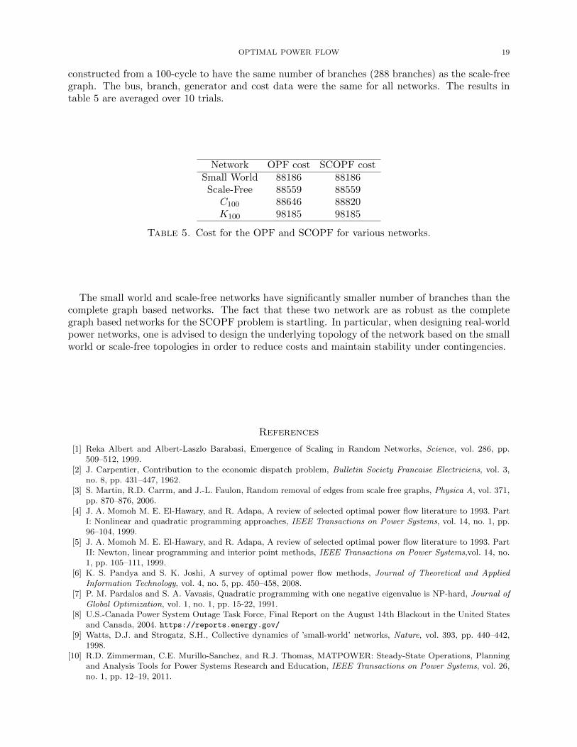
4.4. Comparison of costs of SCOPF for various graphs. In this section we consider therobustness of the small world and scale-free networks under the single e − 1 SCOPF problem. Itturns out that similar to the complete graphs (and unlike the cycles), both the small world andscale-free graphs are surprisingly robust under contingency constraints. In particular, the ratio ofthe minimal cost for the OPF on these networks to the minimal cost for the single e− 1 SCOPF is1. However, the minimal cost for the power flow problems is significantly lower on the small worldand scale-free networks compared to the cost for the corresponding complete graphs with the samenumber of buses.

In table 5 below, we show the cost of the OPF problem and the single e − 1 SCOPF on thesmall world, scale-free, cycle, and complete networks with 100 buses each. The scale-free graphwas constructed with k = 3 starting with the 6-cycle in Figure 4.1. The small world graph was


constructed from a 100-cycle to have the same number of branches (288 branches) as the scale-freegraph. The bus, branch, generator and cost data were the same for all networks. The results intable 5 are averaged over 10 trials.

Network OPF cost SCOPF costSmall World 88186 88186Scale-Free 88559 88559C100 88646 88820K100 98185 98185

Table 5. Cost for the OPF and SCOPF for various networks.

The small world and scale-free networks have significantly smaller number of branches than thecomplete graph based networks. The fact that these two network are as robust as the completegraph based networks for the SCOPF problem is startling. In particular, when designing real-worldpower networks, one is advised to design the underlying topology of the network based on the smallworld or scale-free topologies in order to reduce costs and maintain stability under contingencies.

References

[1] Reka Albert and Albert-Laszlo Barabasi, Emergence of Scaling in Random Networks, Science, vol. 286, pp.509–512, 1999.

[2] J. Carpentier, Contribution to the economic dispatch problem, Bulletin Society Francaise Electriciens, vol. 3,no. 8, pp. 431–447, 1962.

[3] S. Martin, R.D. Carrm, and J.-L. Faulon, Random removal of edges from scale free graphs, Physica A, vol. 371,pp. 870–876, 2006.

[4] J. A. Momoh M. E. El-Hawary, and R. Adapa, A review of selected optimal power flow literature to 1993. PartI: Nonlinear and quadratic programming approaches, IEEE Transactions on Power Systems, vol. 14, no. 1, pp.96–104, 1999.

[5] J. A. Momoh M. E. El-Hawary, and R. Adapa, A review of selected optimal power flow literature to 1993. PartII: Newton, linear programming and interior point methods, IEEE Transactions on Power Systems,vol. 14, no.1, pp. 105–111, 1999.

[6] K. S. Pandya and S. K. Joshi, A survey of optimal power flow methods, Journal of Theoretical and AppliedInformation Technology, vol. 4, no. 5, pp. 450–458, 2008.

[7] P. M. Pardalos and S. A. Vavasis, Quadratic programming with one negative eigenvalue is NP-hard, Journal ofGlobal Optimization, vol. 1, no. 1, pp. 15-22, 1991.

[8] U.S.-Canada Power System Outage Task Force, Final Report on the August 14th Blackout in the United Statesand Canada, 2004. https://reports.energy.gov/

[9] Watts, D.J. and Strogatz, S.H., Collective dynamics of ’small-world’ networks, Nature, vol. 393, pp. 440–442,1998.

[10] R.D. Zimmerman, C.E. Murillo-Sanchez, and R.J. Thomas, MATPOWER: Steady-State Operations, Planningand Analysis Tools for Power Systems Research and Education, IEEE Transactions on Power Systems, vol. 26,no. 1, pp. 12–19, 2011.

https://reports.energy.gov/


Department of Mathematics, Washington State University, Pullman, WA, U.S.AE-mail address: [email protected]

Department of Mathematics, University of Toronto, ON, CanadaE-mail address: [email protected]

Department of Mathematics, University of California Los Angeles, Los Angeles, CA, U.S.AE-mail address: [email protected]

School of Mathematical and Statistical Sciences, Arizona State University, Tempe, AZ, U.S.AE-mail address: [email protected]

Department of Mathematics, University of Toronto, ON, CanadaE-mail address: [email protected]

Department of Applied Mathematics, University of Waterloo, Waterloo, ON, CanadaE-mail address: [email protected]

Documents

Baha Alzalg, Catalina Anghel, Wenying Gan, Qing Huang ... · BAHA ALZALG, CATALINA ANGHEL, WENYING GAN, QING HUANG, MUSTAZEE RAHMAN, AND ALEX SHUM Abstract. The optimal power ow problem