Bag of Visual Words - cs.umd.edu

Bag of Visual Words

Thanks to Svetlana Lazebnik and Andrew Zisserman for the use of some

slides

How many categories?

10,000-30,000

OBJECTS

ANIMALS INANIMATEPLANTS

MAN-MADENATURALVERTEBRATE …..

MAMMALS BIRDS

PIGEONHORSECOW CHAIR

History 1960s – early 1990s: geometry 1990s: appearance Mid-1990s: sliding window Late 1990s: local features Early 2000s: parts-and-shape models Mid-2000s: bags of features Present trends: data-driven methods, context

Local features

D. Lowe (1999, 2004)

RECOGNITION AS AN APPLICATION OF MACHINE LEARNING

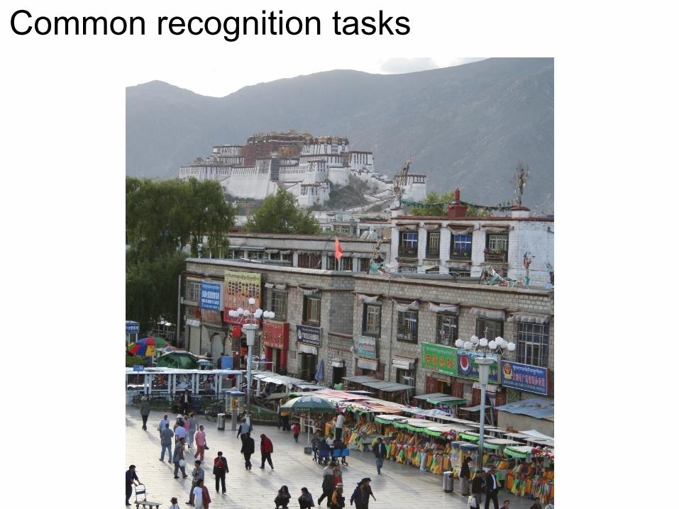
Common recognition tasks

Image classification• outdoor/indoor • city/forest/factory/etc.

Image tagging

• street • people • building • mountain • …

Object detection• find pedestrians

Activity recognition

• walking • shopping • rolling a cart • sitting • talking • …

Image parsing

mountain

buildingtree

banner

marketpeople

street lamp

sky

building

Image descriptionThis is a busy street in an Asian city. Mountains and a large palace or fortress loom in the background. In the foreground, we see colorful souvenir stalls and people walking around and shopping. One person in the lower left is pushing an empty cart, and a couple of people in the middle are sitting, possibly posing for a photograph.

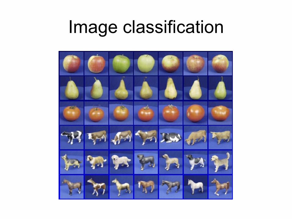
Image classification

Prediction

StepsTraining LabelsTraining

Images

Training

Training

Image Features

Image Features

Testing

Test Image

Learned model

Learned model

Slide credit: D. Hoiem

Traditional recognition pipeline

Hand-designed feature

extraction

Trainable classifier

Image Pixels

• Features are not learned • Trainable classifier is often generic (e.g. SVM)

Object Class

Bags of features

• Orderless document representation: frequencies of words from a dictionary Salton & McGill (1983)

Bags of features: Motivation

Representing a document “in math”Simplest method: bag of words

Represent each document as a vector of word frequencies • Order of words does not matter, just #occurrences

Bag of words Example

the quick brown fox jumps over the lazy dog I am he as you are he as you are me he said the CMSC320 is 189 more CMSCs than the CMSC131

the CMSC320

you he I quick

dog me CMSCs

…

than

2 0 0 0 0 1 1 0 0

…

00 0 2 2 1 0 0 1 0 02 1 0 1 0 0 0 0 1 1

Document 1Document 2Document 3

Term FrequencyTerm frequency: the number of times a term appears in a specific document

• tfij: frequency of word j in document i This can be the raw count (like in the BOW in the last slide):

• tfij ∈ {0,1} if word j appears or doesn’t appear in doc i

• log(1 + tfij) – reduce the effect of outliers • tfij / maxj tfij – normalize by document i’s most frequent

word What can we do with this?

• Use as features to learn a classifier w ! y …!

Defining features From Term FrequencySuppose we are classifying if a document was written by The Beatles or not (i.e., binary classification):

• Two classes y ∈ Y = { 0, 1 } = { not_beatles, beatles } Let’s use tfij ∈ {0,1}, which gives:

Then represent documents with a feature function: f(x, y = not_beatles = 0) = [xT, 0T, 1]T

f(x, y = beatles = 1) = [0T, xT, 1]T

the CMSC320

you he I quick dog me CMSCs

…

than

1 0 0 0 0 1 1 0 0

…

00 0 1 1 1 0 0 1 0 01 1 0 1 0 0 0 0 1 1

x1T =

x2T =

x3T =

y1 = 0y2 = 1y3 = 0

Linear classificationWe have a feature function f(x, y) and a score 𝝍xy = θT f(x, y)

For each class y ∈ { not_beatles, beatles }

Compute the score of the document for that class

And return the class with highest score!

weights

linear classifier

Texture recognition

Universal texton dictionary

histogram

Julesz, 1981; Cula & Dana, 2001; Leung & Malik 2001; Mori, Belongie & Malik, 2001; Schmid 2001; Varma & Zisserman, 2002, 2003; Lazebnik, Schmid & Ponce, 2003

1. Extract local features 2. Learn “visual vocabulary” 3. Quantize local features using visual vocabulary 4. Represent images by frequencies of “visual words”

Traditional features: Bags-of-features

1. Local feature extraction• Sample patches and extract descriptors

Keypoints

patches surrounding keypoints

2. Learning the visual vocabulary

…

Slide credit: Josef Sivic except for the image patches

Extracted descriptors from the training set



Clustering

…

Slide credit: Josef Sivic


Clustering

…


Visual vocabulary

Example visual vocabulary

…

Source: B. Leibe

Appearance codebook


Bag-of-features steps

CLUSTERING• Group a collection of points into clusters

• We have seen “supervised methods”, where the outcome (or response) is based on various predictors.

• In clustering, we want to extract patterns on variables without analyzing a specific response variable.

• This is a form of “unsupervised learning”

CLUSTERING• The points in each cluster are closer to one another and far from the points in

other clusters.

Data Points• Each of the data points belong to some n-dimensional space.

Clusters• The clusters are grouped based on some distance /similarity measurement.

• Two-main types of clustering techniques are:

• point-assignment or k-means • hierarchical or agglomerative

• Sometimes we work with dissimilarity (or distance) measurements.

• First let us discuss the (dis)similarity measurements.

dissimilarity measurements

• We can define dissimilarity between objects as

• The most common distance measure is squared distance

Define dissimilarity, dj(xij, xi′ j)

Given measurements xij for i = 1,…, M observations over j = 1,…, n predictors.

d(xi, xi′ ) =N

∑j=1

dj(xij, xi′ j)

dj(xij, xi′ j) = (xij − xi′ j)2

dissimilarity measurements

• Absolute difference

• For categorical variables, we could set

dj(xij, xi′ j) = |xij − xi′ j |

dj(xij, xi′ j) = 0 if xij = xi′ j

1 otherwise

Clustering techniques

• Two-main types of clustering techniques are:

• point-assignment or k-means

• hierarchical or agglomerative

K-Means Clustering

• A commonly used algorithm to perform clustering

• Assumptions: • Euclidean distance,

• K-means partitions observations into K clusters, with K provided as a parameter.

dii′ = d(xi, xi′ ) =p

∑j=1

(xij − xi′ j)2 = | |xi − xi′ | |2

K-Means Objective function

• We are given an integer k and a set of n data points

we wish to choose k centers C so as to minimize within-cluster dissimilarity.

• The criteria to minimize is the total distance given by each observation to the mean(centroid) of the cluster to which the observation is assigned.

X ⊂ ℝp

W =N

∑i=1

minc∈C

| |xi − c | |2

K-Means - Iterative algorithm

1. Arbitrarily choose an initial k centers

2. For each set the cluster to be the set of points X that are closer to than they are to for all

3. For each , set to be the center of mass of all

points in

4. Repeat Steps 2 and 3 until C no longer changes

i ∈ {1,…, k} Cici cj j ≠ i

i ∈ {1,…, k} ci

Ci : ci =1

|Ci | ∑x∈Ci

x

C = {c1, c2, …, ck}

K-means - picking K

• Minimization, W, It is not a convex criteria, we may not obtain global optima.

• In practice the algorithm is run with multiple initializations (step 1) and the best clustering is used.

Choosing the number of clusters

1. The number of parameters must be determined before running k-means algorithm.

2. There is no clean direct method for choosing the number of clusters to use in the K-means algorithm

Choosing the number of clusters - Elbow method

Picking k - Gap statistic (Hastie et al.)

• Suppose data is clustered into clusters, with denoting the observations in cluster , and

• The sum of pairwise distances for all points in cluster is given by

and

• If is the squared Euclidean distance then is the pooled within-cluster sum of squares around the cluster means.

k

Cr r nr = |Cr |r

Dr = ∑i,i′ ∈Cr

dii′

Wk =k

∑r=1

12nr

Dr

d Wk

C1, C2, …, Ck

https://statweb.stanford.edu/~gwalther/gap

dii′ = d(xi, xi′ ) =p

∑j=1

(xij − xi′ j)2 = | |xi − xi′ | |2

Gap Statistic - Procedure (Tibshirani et al.)

1. Cluster the observed data, varying the total number of clusters from . Obtain

2. Generate reference sets, using uniform distribution or SVD followed by uniform distribution. , with

3. Compute the estimated Gap statistic

4. Let , compute the standard deviation

5. Define . 6. Choose the number of clusters via

k = 1,2,…, KWk

BW*kb b = 1,2,…, B, k = 1,2,…, K

Gap(k) = (1/B)∑b

log(W*kb) − log(Wk)

l = (1/B)∑b

log(W*kb)

sdk = [(1/B)∑b

{log(W*kb) − l}2]1/2

sk = sdk 1 + 1/B

k = smallest k such that Gap(k) ≥ Gap(k + 1) − sk+1

Choosing the number of clusters - Gap statistic

Gap(k) = E[log(W*kb)] − log(Wk)E[log(W*kb)] = l = (1/B)∑

b

log(W*kb)

Choosing the number of clusters - Elbow method

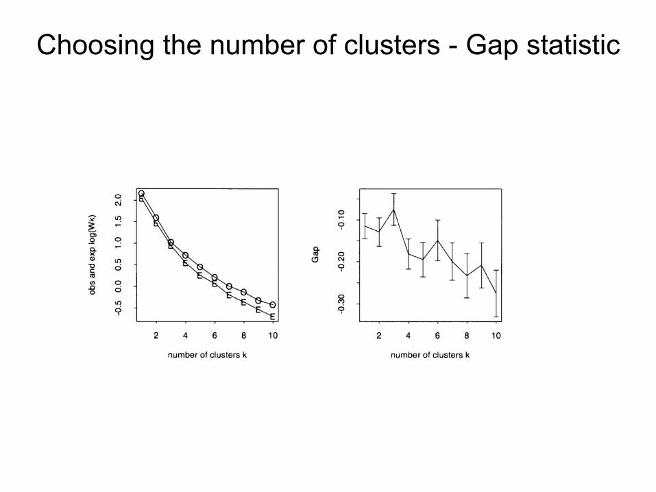
Choosing the number of clusters - Gap statistic


Traditional features: Bags-of-features

1. Local feature extraction• Sample patches and extract descriptors

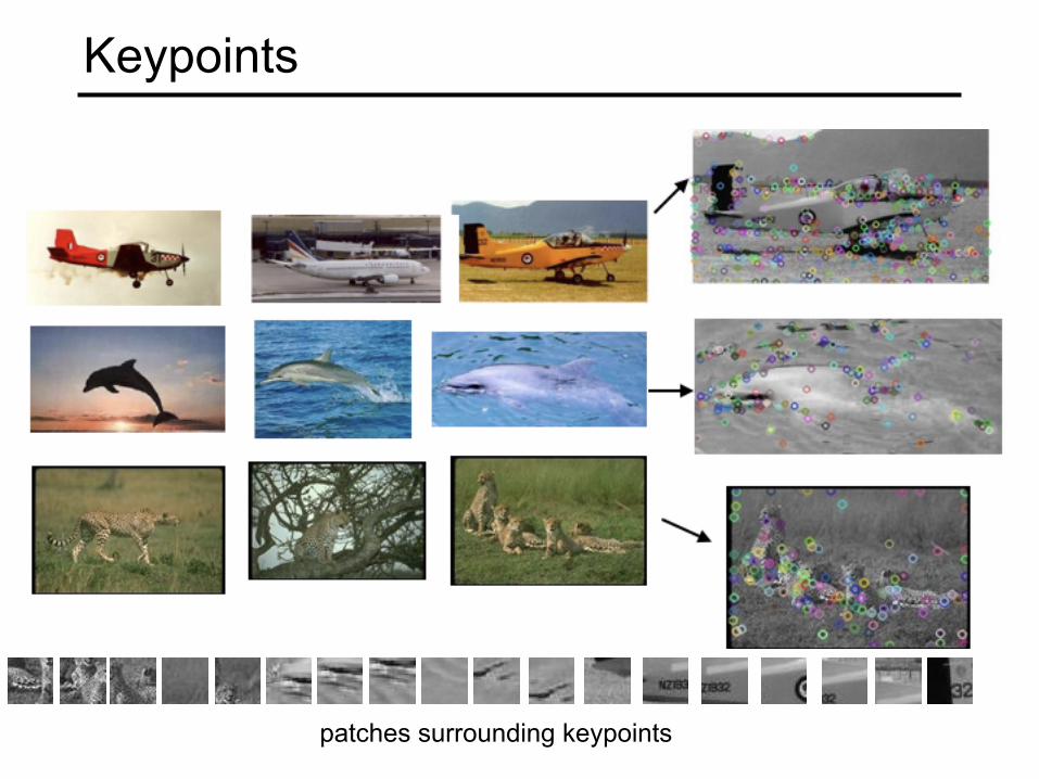
Keypoints



…

Slide credit: Josef Sivic except for the image patches

Extracted descriptors from the training set



Clustering

…



Clustering

…


Visual vocabulary

Example visual vocabulary

…

Source: B. Leibe

Appearance codebook


Bag-of-features steps

Bag-of-features (Visual Words) steps

Generalization• Generalization refers to the ability to correctly

classify never before seen examples • Can be controlled by turning “knobs” that affect

the complexity of the model

Training set (labels known) Test set (labels unknown)

Diagnosing generalization ability• Training error: how does the model perform on the data on

which it was trained? • Test error: how does it perform on never before seen data?

Training error

Test error

Source: D. Hoiem

Underfitting Overfitting

Model complexity HighLow

Err

or

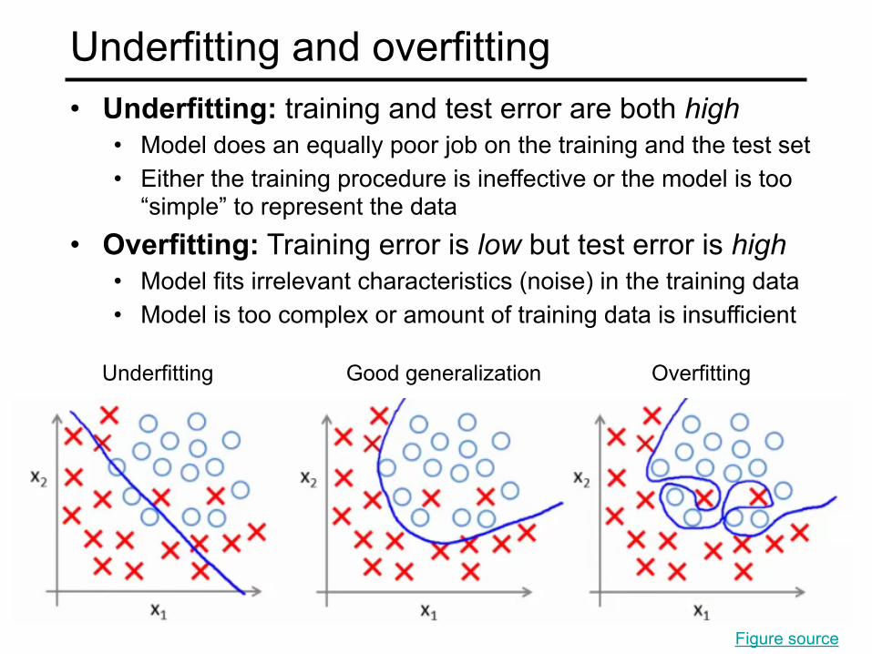
Underfitting and overfitting• Underfitting: training and test error are both high

• Model does an equally poor job on the training and the test set • Either the training procedure is ineffective or the model is too

“simple” to represent the data • Overfitting: Training error is low but test error is high

• Model fits irrelevant characteristics (noise) in the training data • Model is too complex or amount of training data is insufficient

Underfitting OverfittingGood generalization

Figure source

http://www.holehouse.org/mlclass/07_Regularization.html

Effect of training set size

Many training examples

Few training examples

Model complexity HighLow

Test

Err

or

Source: D. Hoiem

Validation• Split the data into training, validation, and test subsets • Use training set to optimize model parameters • Use validation test to choose the best model • Use test set only to evaluate performance

Model complexity

Training set loss

Test set loss

Err

or

Validation set loss

Stopping point

SummaryThe different steps

Documents

Bag of Visual Words - cs.umd.edu