Baeza-Yates–Perleberg Filtering Algorithm

A filtering algorithm for approximate string matching searches the text forfactors having some property that satisfies the following conditions:

1. Every approximate occurrence of the pattern has this property.

2. Strings having this property are reasonably rare.

3. Text factors having this property can be found quickly.

Each text factor with the property is a potential occurrence, which is thenverified for whether it is an actual approximate occurrence.

Filtering algorithms can achieve linear or even sublinear average case timecomplexity.

145

The following lemma shows the property used by the Baeza-Yates–Perlebergalgorithm and proves that it satisfies the first condition.

Lemma 3.23: Let P1P2 . . . Pk+1 = P be a partitioning of the pattern P intok + 1 nonempty factors. Any string S with ed(P, S) ≤ k contains Pi as afactor for some i ∈ [1..k + 1].

Proof. Each single symbol edit operation can change at most one of thepattern factors Pi. Thus any set of at most k edit operations leaves at leastone of the factors untouched.

146

The algorithm has two phases:

Filtration: Search the text T for exact occurrences of the pattern factors Pi.Using the Aho–Corasick algorithm this takes O(n) time for a constantalphabet.

Verification: An area of length O(m) surrounding each potential occurrencefound in the filtration phase is searched using the standard dynamicprogramming algorithm in O(m2) time.

The worst case time complexity is O(m2n), which can be reduced to O(mn)by combining any overlapping areas to be searched.

147

Let us analyze the average case time complexity of the verification phase.

• The best pattern partitioning is as even as possible. Then each patternfactor has length at least r = bm/(k + 1)c.

• The expected number of exact occurrences of a random string oflength r in a random text of length n is at most n/σr.

• The expected total verification time is at most

O(m2(k + 1)n

σr

)≤ O

(m3n

σr

).

This is O(n) if r ≥ 3 logσm.

• The condition r ≥ 3 logσm is satisfied when (k + 1) ≤ m/(3 logσm+ 1).

Theorem 3.24: The average case time complexity of theBaeza-Yates–Perleberg algorithm is O(n) when k ≤ m/(3 logσm+ 1)− 1.

148

Many variations of the algorithm have been suggested:

• The filtration can be done with a different multiple exact stringmatching algorithm:

– The first algorithm of this type by Wu and Manber used anextension of the Shift-And algorithm.

– An extension of BDM achieves O(nk(logσm)/m) average casesearch time. This is sublinear for small enough k.

– An extension of the Horspool algorithm is very fast in practice forsmall k and large σ.

• Using a technique called hierarchical verification, the averageverification time for a single potential occurrence can be reduced toO((m/k)2).

A filtering algorithm by Chang and Marr has average case time complexityO(n(k + logσm)/m), which is optimal.

149

Summary: Approximate String Matching

We have seen two main types of algorithms for approximate string matching:

• Basic dynamic programming time complexity is O(mn). The timecomplexity can be improved to O(kn) using diagonal monotonicity, andto O(ndm/we) using bitparallelism.

• Filtering algorithms can improve average case time complexity and arethe fastest in practice when k is not too large.

Other algorithms worth mentioning are those based on automata:

• Algorithms based on bit-parallel simulation of non-deterministicautomata were mentioned briefly.

• A deterministic automaton can find occurrences in O(n) time, but thesize of the automaton can be exponential in m and too big to bepractical.

Similar techniques can be useful for other variants of edit distance but notalways straightforwardly.

150

4. Suffix Trees and Arrays

Let T = T [0..n) be the text. For i ∈ [0..n], let Ti denote the suffix T [i..n).Furthermore, for any subset C ∈ [0..n], we write TC = Ti | i ∈ C. Inparticular, T[0..n] is the set of all suffixes of T .

Suffix tree and suffix array are search data structures for the set T[0..n].

• Suffix tree is a compact trie for T[0..n].

• Suffix array is an ordered array for T[0..n].

They support fast exact string matching on T :

• A pattern P has an occurrence starting at position i if and only if P is aprefix of Ti.

• Thus we can find all occurrences of P by a prefix search in T[0..n].

A data structure supporting fast string matching is called a text index.

There are numerous other applications too, as we will see later.

151

The set T[0..n] contains |T[0..n]| = n+ 1 strings of total length||T[0..n]|| = Θ(n2). It is also possible that ΣLCP (T[0..n]) = Θ(n2), for example,when T = an or T = XX for any string X.

• A basic trie has Θ(n2) nodes for most texts, which is too much. Even aleaf path compacted trie can have Θ(n2) nodes, for example whenT = XX for a random string X.

• A compact trie with O(n) nodes and an ordered array with n+ 1 entrieshave linear size.

• A compact ternary trie and a string binary search tree have O(n) nodestoo. However, the construction algorithms and some other algorithmswe will see are not straightforward to adapt for these data structures.

Even for a compact trie or an ordered array, we need a specializedconstruction algorithm, because any general construction algorithm wouldneed Ω(ΣLCP (T[0..n])) time.

152

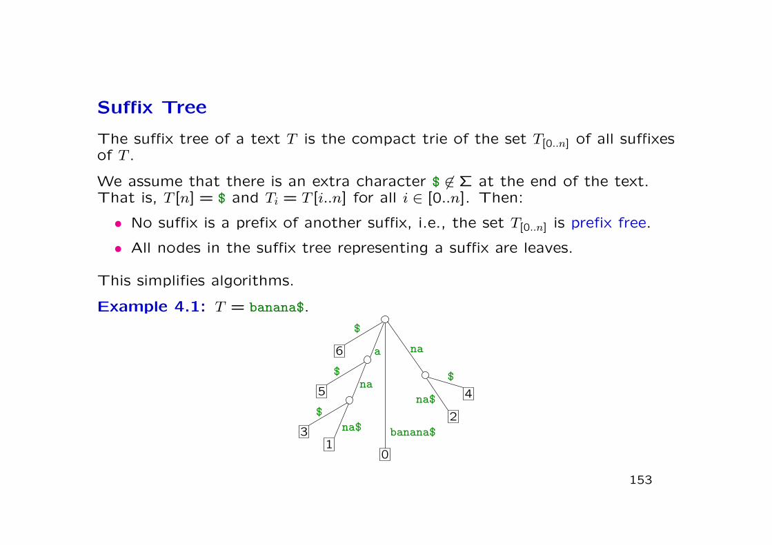
Suffix Tree

The suffix tree of a text T is the compact trie of the set T[0..n] of all suffixesof T .

We assume that there is an extra character $ 6∈ Σ at the end of the text.That is, T [n] = $ and Ti = T [i..n] for all i ∈ [0..n]. Then:

• No suffix is a prefix of another suffix, i.e., the set T[0..n] is prefix free.

• All nodes in the suffix tree representing a suffix are leaves.

This simplifies algorithms.

Example 4.1: T = banana$.

13

5

6

2

4

0

$

$

$

na$

na$

na

na$

banana$

a

153

As with tries, there are many possibilities for implementing the childoperation. We again avoid this complication by assuming that σ is constant.Then the size of the suffix tree is O(n):

• There are exactly n+ 1 leaves and at most n internal nodes.

• There are at most 2n edges. The edge labels are factors of the textand can be represented by pointers to the text.

Given the suffix tree of T , all occurrences of P in T can be found in timeO(|P |+ occ), where occ is the number of occurrences.

154

Brute Force Construction

Let us now look at algorithms for constructing the suffix tree. We start witha brute force algorithm with time complexity Θ(ΣLCP (T[0..n])). Later wewill modify this algorithm to obtain a linear time complexity.

The idea is to add suffixes to the trie one at a time starting from thelongest suffix. The insertion procedure is essentially the same as we saw inAlgorithm 1.2 (insertion into trie) except it has been modified to work on acompact trie instead of a trie.

155

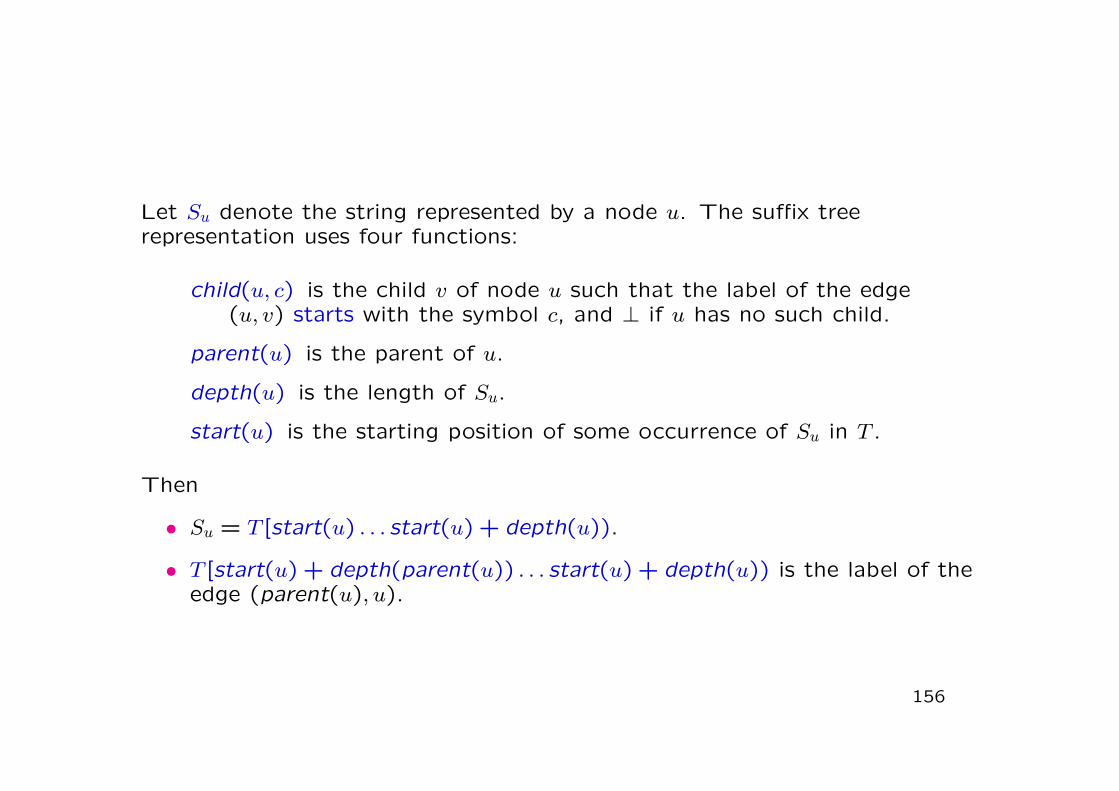
Let Su denote the string represented by a node u. The suffix treerepresentation uses four functions:

child(u, c) is the child v of node u such that the label of the edge(u, v) starts with the symbol c, and ⊥ if u has no such child.

parent(u) is the parent of u.

depth(u) is the length of Su.

start(u) is the starting position of some occurrence of Su in T .

Then

• Su = T [start(u) . . . start(u) + depth(u)).

• T [start(u) + depth(parent(u)) . . . start(u) + depth(u)) is the label of theedge (parent(u), u).

156

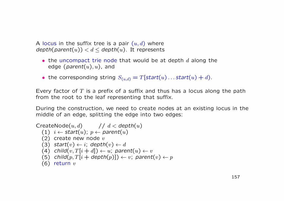
A locus in the suffix tree is a pair (u, d) wheredepth(parent(u)) < d ≤ depth(u). It represents

• the uncompact trie node that would be at depth d along theedge (parent(u), u), and

• the corresponding string S(u,d) = T [start(u) . . . start(u) + d).

Every factor of T is a prefix of a suffix and thus has a locus along the pathfrom the root to the leaf representing that suffix.

During the construction, we need to create nodes at an existing locus in themiddle of an edge, splitting the edge into two edges:

CreateNode(u, d) // d < depth(u)(1) i← start(u); p← parent(u)(2) create new node v(3) start(v)← i; depth(v)← d(4) child(v, T [i+ d])← u; parent(u)← v(5) child(p, T [i+ depth(p)])← v; parent(v)← p(6) return v

157

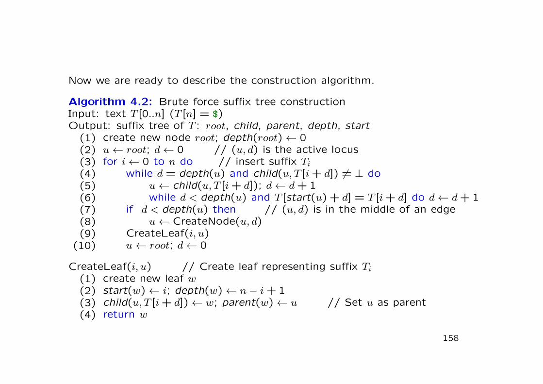
Now we are ready to describe the construction algorithm.

Algorithm 4.2: Brute force suffix tree constructionInput: text T [0..n] (T [n] = $)Output: suffix tree of T : root, child, parent, depth, start

(1) create new node root; depth(root)← 0(2) u← root; d← 0 // (u, d) is the active locus(3) for i← 0 to n do // insert suffix Ti(4) while d = depth(u) and child(u, T [i+ d]) 6= ⊥ do(5) u← child(u, T [i+ d]); d← d+ 1(6) while d < depth(u) and T [start(u) + d] = T [i+ d] do d← d+ 1(7) if d < depth(u) then // (u, d) is in the middle of an edge(8) u← CreateNode(u, d)(9) CreateLeaf(i, u)

(10) u← root; d← 0

CreateLeaf(i, u) // Create leaf representing suffix Ti(1) create new leaf w(2) start(w)← i; depth(w)← n− i+ 1(3) child(u, T [i+ d])← w; parent(w)← u // Set u as parent(4) return w

158

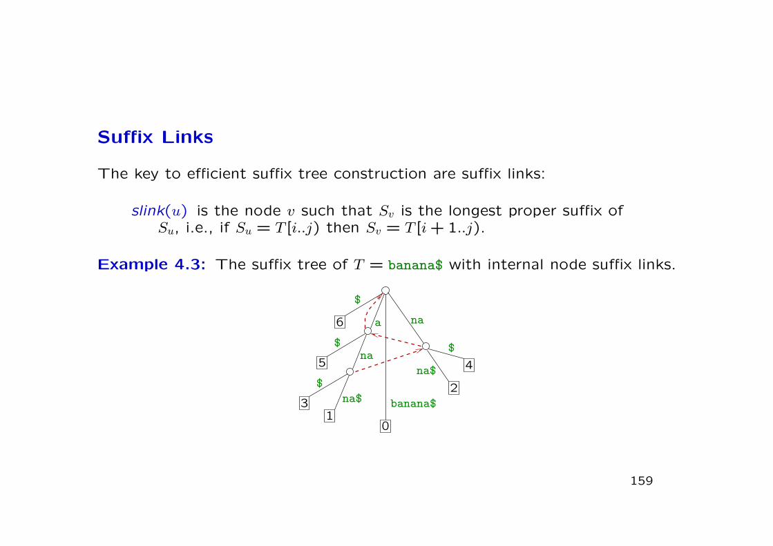
Suffix Links

The key to efficient suffix tree construction are suffix links:

slink(u) is the node v such that Sv is the longest proper suffix ofSu, i.e., if Su = T [i..j) then Sv = T [i+ 1..j).

Example 4.3: The suffix tree of T = banana$ with internal node suffix links.

13

5

6

2

4

0

$

$

$

na$

na$

na

na$

banana$

a

159

Suffix links are well defined for all nodes except the root.

Lemma 4.4: If the suffix tree of T has a node u representing T [i..j) for any0 ≤ i < j ≤ n, then it has a node v representing T [i+ 1..j).

Proof. If u is the leaf representing the suffix Ti, then v is the leafrepresenting the suffix Ti+1.

If u is an internal node, then it has two child edges with labels starting withdifferent symbols, say a and b, which means that T [i..j)a and T [i..j)b areboth factors of T . Then, T [i+ 1..j)a and T [i+ 1..j)b are factors of T too,and thus there must be a branching node v representing T [i+ 1..j).

Usually, suffix links are needed only for internal nodes. For root, we defineslink(root) = root.

160

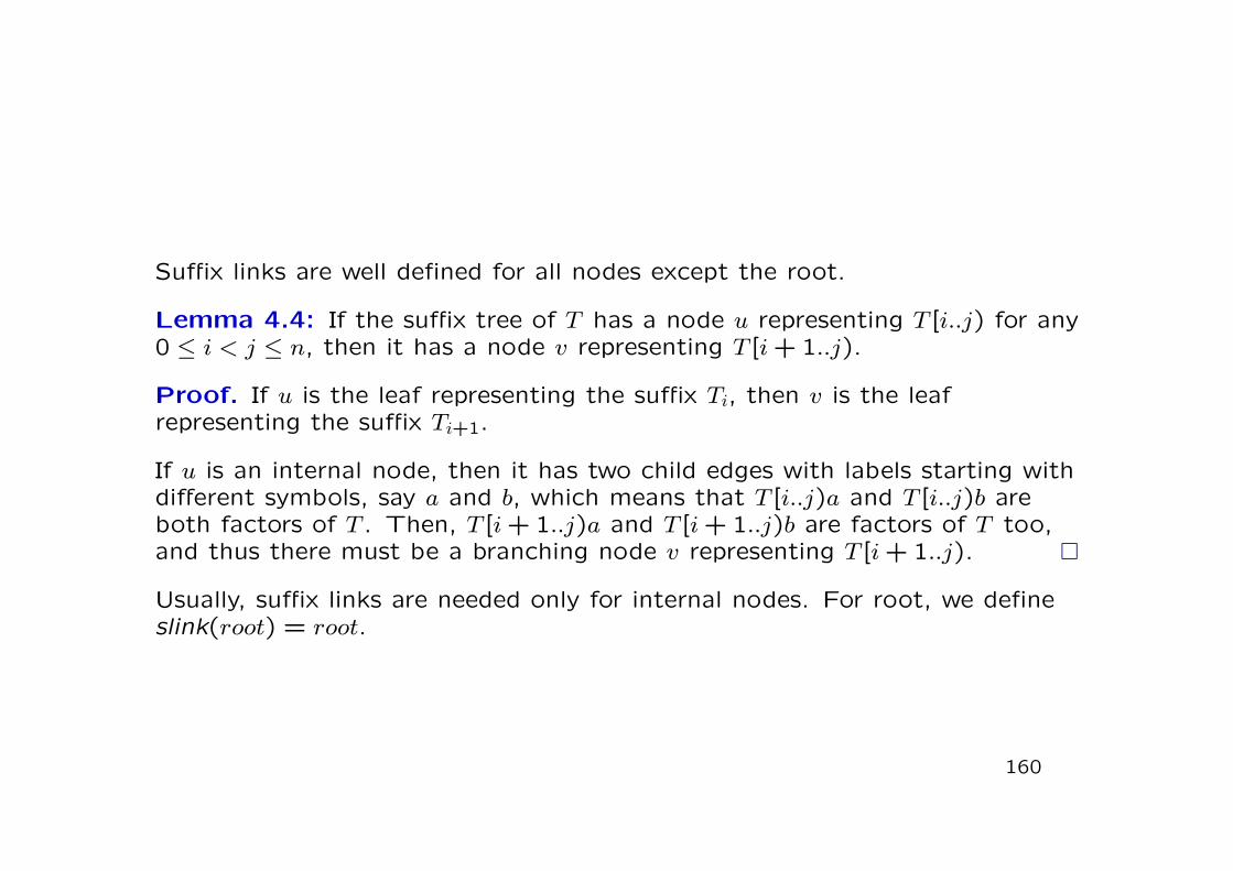
Suffix links are the same as Aho–Corasick failure links but Lemma 4.4ensures that depth(slink(u)) = depth(u)− 1. This is not the case for anarbitrary trie or a compact trie.

Suffix links are stored for compact trie nodes only, but we can define andcompute them for any locus (u, d):

slink(u, d)(1) v ← slink(parent(u))(2) while depth(v) < d− 1 do(3) v ← child(v, T [start(u) + depth(v) + 1])(4) return (v, d− 1)

parent(u)

(u, d)

uslink(u)

slink(u, d)

slink(parent(u))

161

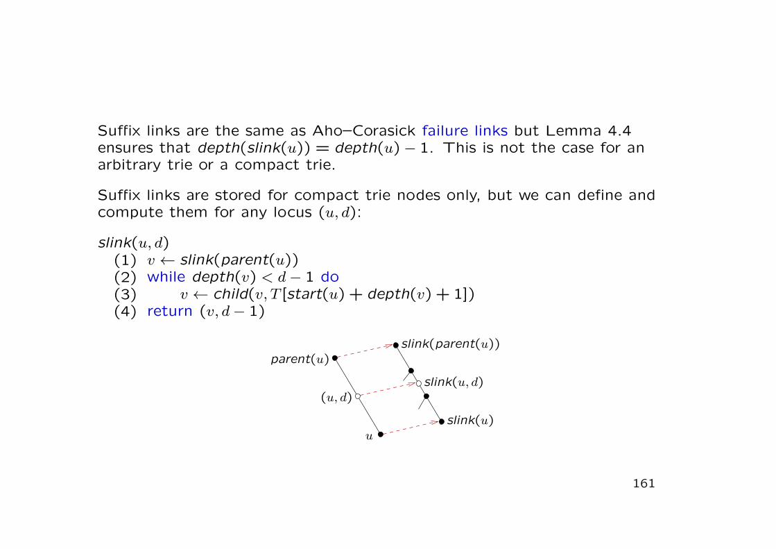
The same idea can be used for computing the suffix links during or after thebrute force construction.

ComputeSlink(u)(1) d← depth(u)(2) v ← slink(parent(u))(3) while depth(v) < d− 1 do(4) v ← child(v, T [start(u) + depth(v) + 1])(5) if depth(v) > d− 1 then // no node at (v, d− 1)(6) v ← CreateNode(v, d− 1)(7) slink(u)← v

The procedure CreateNode(v, d− 1) sets slink(v) = ⊥.

The algorithm uses the suffix link of the parent, which must have beencomputed before. Otherwise the order of computation does not matter.

162

The creation of a new node on line (6) never happens in a fully constructedsuffix tree, but during the brute force algorithm the necessary node may notexist yet:

• If a new internal node ui was created during the insertion of the suffixTi, there exists an earlier suffix Tj, j < i that branches at ui into adifferent direction than Ti.

• Then slink(ui) represents a prefix of Tj+1 and thus exists at least as alocus on the path labelled Tj+1. However, it may be that it does notbecome a branching node until the insertion of Ti+1.

• In such a case, ComputeSlink(ui) creates slink(ui) a moment before itwould otherwise be created by the brute force construction.

163

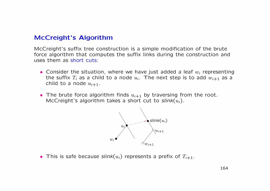
McCreight’s Algorithm

McCreight’s suffix tree construction is a simple modification of the bruteforce algorithm that computes the suffix links during the construction anduses them as short cuts:

• Consider the situation, where we have just added a leaf wi representingthe suffix Ti as a child to a node ui. The next step is to add wi+1 as achild to a node ui+1.

• The brute force algorithm finds ui+1 by traversing from the root.McCreight’s algorithm takes a short cut to slink(ui).

slink(ui)ui

wiwi+1

ui+1

• This is safe because slink(ui) represents a prefix of Ti+1.

164

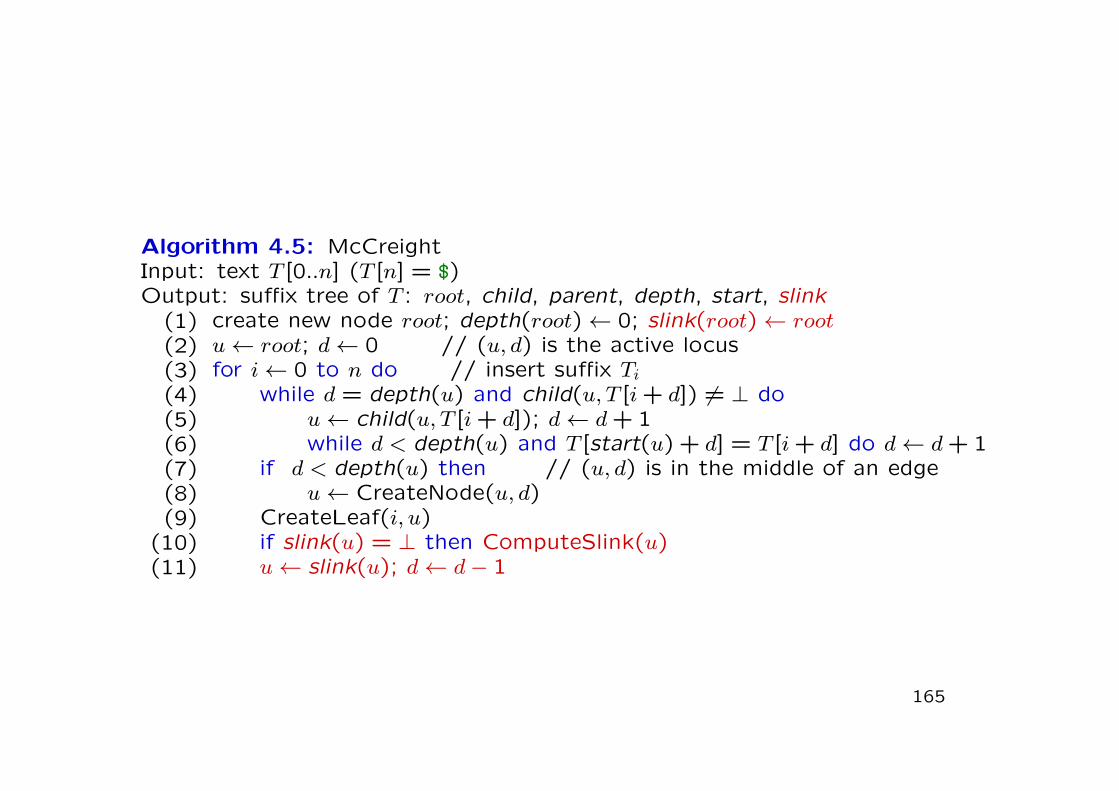
Algorithm 4.5: McCreightInput: text T [0..n] (T [n] = $)Output: suffix tree of T : root, child, parent, depth, start, slink

(1) create new node root; depth(root)← 0; slink(root)← root(2) u← root; d← 0 // (u, d) is the active locus(3) for i← 0 to n do // insert suffix Ti(4) while d = depth(u) and child(u, T [i+ d]) 6= ⊥ do(5) u← child(u, T [i+ d]); d← d+ 1(6) while d < depth(u) and T [start(u) + d] = T [i+ d] do d← d+ 1(7) if d < depth(u) then // (u, d) is in the middle of an edge(8) u← CreateNode(u, d)(9) CreateLeaf(i, u)

(10) if slink(u) = ⊥ then ComputeSlink(u)(11) u← slink(u); d← d− 1

165

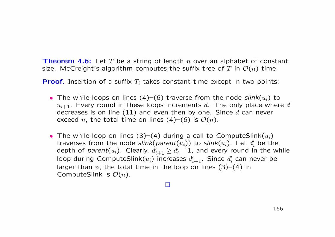
Theorem 4.6: Let T be a string of length n over an alphabet of constantsize. McCreight’s algorithm computes the suffix tree of T in O(n) time.

Proof. Insertion of a suffix Ti takes constant time except in two points:

• The while loops on lines (4)–(6) traverse from the node slink(ui) toui+1. Every round in these loops increments d. The only place where ddecreases is on line (11) and even then by one. Since d can neverexceed n, the total time on lines (4)–(6) is O(n).

• The while loop on lines (3)–(4) during a call to ComputeSlink(ui)traverses from the node slink(parent(ui)) to slink(ui). Let d′i be thedepth of parent(ui). Clearly, d′i+1 ≥ d′i − 1, and every round in the whileloop during ComputeSlink(ui) increases d′i+1. Since d′i can never belarger than n, the total time in the loop on lines (3)–(4) inComputeSlink is O(n).

166

There are other linear time algorithms for suffix tree construction:

• Weiner’s algorithm was the first. It inserts the suffixes into the tree inthe opposite order: Tn, Tn−1, . . . , T0.

• Ukkonen’s algorithm constructs suffix tree first for T [0..1) then forT [0..2), etc.. The algorithm is structured differently, but performsessentially the same tree traversal as McCreight’s algorithm.

• All of the above are linear time only for constant alphabet size.Farach’s algorithm achieves linear time for an integer alphabet ofpolynomial size. The algorithm is complicated and unpractical.

167