Embed Size (px)
Citation preview
i
BACTERIOLOGICAL ANALYSIS OF FAECAL POLLUTION AND SOLAR RADIATION
DISINFECTION OF DOMESTIC WATER SOURCES WITHIN LAKE NAIVASHA
BASIN, KENYA
OSCAR OMONDI DONDE
A Thesis Submitted to the Graduate School in Partial Fulfilment for the Requirements of the
Master of Science Degree in Limnology of Egerton University
EGERTON UNIVERSITY
DECEMBER, 2012
ii
DECLARATION AND RECOMMENDATION
DECLARATION
This thesis is my original work and has not been submitted or presented for examination in any
other institution.
Mr. O. O. Donde
SM18/2524/09
Signature: ______________________ Date: ________________________
RECOMMENDATION
This work has been presented for examination with our approval as university supervisors
Dr. A. W. Muia
Egerton University
Signature: ________________________ Date: __________________________
Prof. W. A. Shivoga
Masinde Muliro University of Science and Technology
Signature: ________________________ Date: __________________________

iii
ACKNOWLEDGEMENT
I am very grateful to the International Developement Research Council (IDRC) through Lake
Naivasha Sustainability Project for financing this research. I whole heartedly appreciate the
patience, tolerance and goodwill of my supervisors; Dr. A. W. Muia and Prof. A. W. Shivoga for
guiding me through the proposal formulation, research as well as thesis write-up. I am also
grateful to Egerton University for giving me facilities to study and carry out the research. My
sincere thanks also go to all lecturers especially those from Egerton University, Department of
Biological Sciences for their relevant academic guidance and support. I am particularly indebted
to Dr. Adiel Magana, Dr. Steve Omondi and Dr. Nzula Kitaka for allocating me working space
and equipments for this study. In addition, I appreciate support from Dr. C. M’Erimba, Dr. A. W.
Yasindi and Dr. J. Kipkemboi for the knowledge they imparted on me which enable me to have
the ability to pursue this study. Their support and assistance during the proposal write-up is also
acknowledged. I also acknowledge Professor Robert Metcalf of the University of California for
providing water pasteurization kit used in this study. All the financial and moral support from
my parents, brothers, sisters and friends are also appreciated. I also thank in a special way the
following colleagues from Egerton University; Ms Pauline Macharia, Mr Elick Otachi, Mr Ken
Ochieng’, Mrs Rosemary and Mr Outa for their assistance and moral support which greatly
contributed to the success of this study. Special thanks to my best friend Lucy Wanga for the
patience she showed during the entire time I was away either in Naivasha or in Canada, I also
appreciate the fact that she was able to dedicate significant part of her time to provide a helping
hand in the laboratory work. The support from the following people and institution is also
appreciated; Water Resource Management Authority (WRMA) Naivasha Office, Naivasha Water
and Sanitation Company (NAWASCO) staff, owners of households, vendors and boreholes. It
was through their authority that I managed to access and get water samples from the boreholes,
rivers and lake. The assistance and support by members from Faculty of Science at Western
University-Canada is also very much appreciated. In particular, thanks to Professor Charlie Trick
and Dr. Irena Creed for their contribution towards the success of this study. Above all, my
gratitude goes to the Lord God and Almighty Father for having guided, blessed and protected me
during the entire research period, it was a tough and long journey, but through his grace I
managed to sail through successfully.

iv
DEDICATION
I dedicate this work to my late mum, Mrs. Mary Donde,
Her last words of encouragement kept ringing in my mind and propelled me to this end.
―Mama‖ rest in eternal peace.
v
ABSTRACT
There is an increase in exposure of water sources to faecal contamination as a result of
expanding anthropogenic activities in Lake Naivasha basin in Kenya. This contamination
exposes water users in the region to a variety of health risks. This study investigated faecal
pollution of community water sources (lake, rivers and boreholes) within Lake Naivasha basin
through determination of the concentrations of total coliforms, Escherichia coli, intestinal
enterococci, Clostridium perfringens and heterotrophic bacteria in various water sources using
Membrane Filtration Technique (MFT) and Heterotrophic Plate Count (HPC) procedures. The
potential of solar pasteurization in disinfecting domestic water was also explored by heating
known volumes of water samples in a black solar box cooker at given time intervals. In addition,
determination of E. coli to intestinal enterococci ratio was used in faecal pollution source
tracking. Physico-chemical parameters were measured in situ for all water sources. Data was
analysed for mean variation using Statistical Package for Social Sciences (SPSS) version 17
software. Surface water sources gave higher values for all microbiological parameters than
borehole sources. Borehole direct sources showed no significant variation for all microbial
parameters (E. coli, total coliform, intestinal enterococci, C. perfringens and HPC) with respect
to sampling sites, the same was also observed in borehole at the Points of Access (POA). Surface
water sources on the other hand, showed significant spatial variation for all microbial parameters
(P<0.05). Samples from borehole POA, households in Karagita, Mirera and Kamere villages and
vendors showed no significant variation for all the microbial parameters. The use of solar
radiation in water disinfection showed that temperature of 75 0C attained after 30 minutes from
pasteurization point completely eliminated E. coli and total coliforms from all the water sources.
E. coli to intestinal enterococci density ratios from all the water sources were closer to 0.7;
showing that non-human warm blooded animals were the most possible sources of faecal
pollution into these water sources. In conclusion, there was faecal contamination of domestic
water sources in Lake Naivasha basin and poor human handling practices contributed to further
deterioration of the water quality. The use of solar radiation can be recommended as a cost-
effective method of disinfecting water for domestic consumption to reduce likely incidences of
waterborne diseases. Use of other methods such as ribotyping is also recommended in tracking
the possible sources of faecal pollution into water sources in Lake Naivasha Basin.
vi
TABLE OF CONTENTS
DECLARATION AND RECOMMENDATION ............................................................................... ii
ACKNOWLEDGEMENT ................................................................................................................. iii
DEDICATION ................................................................................................................................... iv
ABSTRACT ........................................................................................................................................ v
TABLE OF CONTENTS ................................................................................................................... vi
LIST OF TABLES .............................................................................................................................. x
LIST OF FIGURES ........................................................................................................................... xi
LIST OF PLATES ............................................................................................................................ xii
ABBREVIATIONS AND ACRONYMS ......................................................................................... xiii
CHAPTER ONE ................................................................................................................................. 1
INTRODUCTION .............................................................................................................................. 1
1.1 Background information ............................................................................................................. 1
1.2 Statement of the problem ............................................................................................................ 4
1.3 Objectives ................................................................................................................................... 5
1.3.1 Broad objective ................................................................................................................... 5
1.3.2 Specific objectives .............................................................................................................. 5
1.4 Hypotheses .................................................................................................................................. 5
1.5 Justification ................................................................................................................................. 6
CHAPTER TWO ................................................................................................................................ 7
LITERATURE REVIEW ................................................................................................................... 7
2.1 Introduction to ecosystem health................................................................................................. 7
2.2 Importance of water borne diseases ............................................................................................. 7
2.3 Water quality monitoring through IWRM ................................................................................. 9
2.4 Sources and routes of water contamination .............................................................................. 10
vii
2.5 Bacterial indicators of faecal pollution ....................................................................................... 10
2.5.1 Coliform bacteria .............................................................................................................. 11
2.5.2 Thermotolerant coliform bacteria and Escherichia coli ...................................................... 12
2.5.3 Clostridium perfringens .................................................................................................... 13
2.5.4 Enterococci as indicators of faecal pollution ...................................................................... 14
2.5.5 Heterotrophic plate count .................................................................................................. 14
2.6 Bacteriological water quality analyses methods ......................................................................... 14
2.6.1 Membrane filtration technique........................................................................................... 14
2.6.2 Most probable number ...................................................................................................... 15
2.6.3 Flow cytometry ................................................................................................................. 16
2.7 Effects of human handling practices on the quality of water ...................................................... 16
2.8 Source tracking for faecal contamination ................................................................................... 17
2.9 Solar pasteurization ................................................................................................................... 18
CHAPTER THREE .......................................................................................................................... 20
MATERIALS AND METHODS ...................................................................................................... 20
3.1 Study area................................................................................................................................ 20
3.1.1 Geographical location ....................................................................................................... 20
3.1.2 Rainfall and temperature patterns ...................................................................................... 20
3.1.3 Water sources .................................................................................................................... 20
3.2 Study design .............................................................................................................................. 22
3.2.1 Sampling ........................................................................................................................... 22
3.2.2 Description of sampling sites and water sources ................................................................ 23
3.3 Bacteriological samples analysis ................................................................................................ 27
3.3.1 Heterotrophic plate count procedure .................................................................................. 27
viii
3.3.2 Membrane filtration technique........................................................................................... 28
3.4 Solar disinfection....................................................................................................................... 28
3.5 Tracking of faecal contamination sources .................................................................................. 29
3.6 Data analysis ............................................................................................................................. 29
CHAPTER FOUR ............................................................................................................................ 31
RESULTS.......................................................................................................................................... 31
4.1 Physical and chemical parameters ............................................................................................. 31
4.2. Microbiological parameters ...................................................................................................... 34
4.2.1 Boreholes .......................................................................................................................... 34
4.2.2 Surface sources ................................................................................................................. 39
4.3 Effects of human water handling practices on its microbial quality ............................................ 42
4.4 Relationship between faecal contamination indicators and physicochemical parameters ............ 44
4.5 Classification of water sources .................................................................................................. 45
4.6 Faecal contamination source tracking ........................................................................................ 47
4.7 Solar disinfection....................................................................................................................... 47
CHAPTER FIVE .............................................................................................................................. 50
DISCUSSION.................................................................................................................................... 50
5.1 Physicochemical parameters ...................................................................................................... 50
5.2 Microbiological Parameters ...................................................................................................... 51
5.3 Solar radiation disinfection ........................................................................................................ 55
CHAPTER SIX ................................................................................................................................. 58
CONCLUSION AND RECOMMENDATION ................................................................................ 58
6.1 Conclusion ................................................................................................................................ 58
6.2 Recommendations ..................................................................................................................... 58

ix
REFERENCES ................................................................................................................................. 60
APPENDICES................................................................................................................................... 67
x
LIST OF TABLES
Table 1: Examples of waterborne diseases………………………………………………………8
Table 2: Description and location of study sites………………………………………………..23
Table 3: Values for physical and chemical parameters from different water sources, households
(HH) and vendors………………………………………………………………………………...33
Table 4: Spatial variation of physico-chemical parameters in borehole direct water
Sources…………………………………………………………………………………………...34
Table 5: Spatial variation of physico-chemical parameters in the borehole points of use
sources……………………………………………………………………………………………34
Table 6: Spatial variation of physico-chemical parameters in surface water sources…………34
Table 7: Spatial variation on the microbial parameters for the borehole points of access
sources……………………………………………………………………………………………36
Table 8: Spatial variation of microbiological parameters within the surface sources………….41
Table 9: Values of microbiological parameters in samples from vendors and
households………………………………………………………………………………………..42
Table 10: Spatial variation on microbiological quality of water at different domains…………44
Table 11: Correlation between microbiological and physicochemical parameters in borehole direct
sources…………………………………………………………………………………………………..44
Table 12: Correlation between microbiological and physico-chemical parameters in borehole point of
access sources…………………………………………………………………………………………..45
Table 13: Correlation between microbiological and physico-chemical parameters in surface sources………………………………………………………………………………………………….45
Table 14: Summary of water source classes within Lake Naivasha area based on contamination
levels..……………………………………………………………………………………………46
Table 15: Mean values and ratios of E. coli to intestinal enterococci in borehole and surface
sources……………………………………………………………………………………………47
Table 16: Response of total coliforms and E. coli to solar pasteurization at different duration of
time and for different water sources and volumes………………………………………………48
xi
LIST OF FIGURES
Figure 1: Conceptual framework on water quality monitoring through IWRM
approach…………………………………………………………………………………………...9
Figure 2: Potential drinking water contamination pathways between source and
household………………………………………………………………………………………...17
Figure 3: Map of Lake Naivasha basin showing the study sites.………………………………21
Figure 4: Densities of faecal contamination indicators in borehole direct water sources………35
Figure 5: Densities of indicators of faecal contamination in boreholes points of access
sources……………………………………………………………………………………………36
Figure 6: Densities of faecal contamination indicators in borehole-direct sources verses borehole
points of access………………..…………………………………………………………………37
Figure 7: Temporal patterns of microbiological indicators of faecal pollution in BH-DIR sources
during the sampling time………………………………………………………………………...38
Figure 8: Temporal pattern of microbiological indicators of faecal pollution in BH-POU
sources……………………………………………………………………………………………39
Figure 9: Densities of faecal contamination indicators in water samples from surface
sources……………………………………………………………………………………………40
Figure 10: Trends of microbiological indicators of faecal pollution in surface water sources
during the sampling time………………………………………………………………………...41
Figure 11: Densities of faecal contamination indicators in water at different domains………...43
Figure 12: Response of faecal indicators to solar pasteurization on water samples from Karagita
Borehole V point of access (KRBHV-POA)……………………………………………………48
Figure 13: Response of faecal indicators to solar pasteurization on water samples from Lake
Naivasha…………………………………………………………………………………………49
Figure 14: Response of faecal indicators to solar pasteurization on water samples from River
Gilgil...…………………………………………………………………………………………...49
xii
LIST OF PLATES
Plate 1: Some of the activities enhancing the transmission and spread of WBD within Lake
Naivasha basin…………………………………………………………………………………….4
Plate 2: Direct borehole sites; (a) DCK and (b) KRBH III……………………………………..23
Plate 3: Borehole points of access; (a) KRBH-II and (b) KRBH-V……………………………24
Plate 4: River Malewa sampling site (MAL RVR)……………………………………………...24
Plate 5: River Gilgil sampling sites……………………………………………………………...25
Plate 6: Sampling site within Lake Naivasha at Kamere Beach (KMBEACH)………………..25
Plate 7: Water sampling from vendors’ domain………………………………………………...26
Plate 8: Water storage container at the household domain……………………………………...26
Plate 9: Colony forming units for Heterotrophic Plate Counts………………………………….27
Plate 10: Plates of MFT showing CFUs…………………………………………………………28
Plate11: Solar pasteurization kit………………………………………………………………...29
xiii
ABBREVIATIONS AND ACRONYMS
APHA American Public Health Association
BH DIR Borehole Direct
BOD Biological Oxygen Demand
BST Bacterial Source Tracking
C. perfrigens Clostridium perfringens
CP Clostridium perfringens
DO Dissolved Oxygen
E. coli Escherichia coli
EC Escherichia coli
FC Faecal Coliforms
HPC Heterotrophic Plate Count
IE Intestinal Enterococci
IWRM Integrated Water Resource Management
LSD Least Significance Difference
MFT Membrane Filtration Technique
MPN Most Probable Number
MTF Multiple Tube Fermentation
NAWASCO Naivasha Water and Sanitation Company
NEMA National Environmental Management Authority
BH POA Borehole Points of Access
SBC Solar Box Cooker
TC Total coliforms
US EPA United States Environmental Protection Agency
WAPI Water Pasteurization Indicator
WBD Waterborne Diseases
WHO World Health Organization
WRMA Water Resource Management Authority
1
CHAPTER ONE
INTRODUCTION
1.1 Background information
Naivasha is one of the fastest growing towns in Kenya. Its growth is enhanced by the increasing
horticulture farming and associated businesses, especially floriculture around the lake Naivasha
(JICA, 2003). In addition, the area surrounding the lake offers a mild climate and natural beauty
that has attracted tourism. Lake Naivasha also supports a productive fishery that provides jobs
and income as well as being an important source of fish protein for local communities. Tourism
activities in the region have contributed to growth in population in Naivasha District. In addition,
rural to urban migration as a result of falling farm incomes from traditional cash crops, and
commercial enterprises and good prospects for job opportunities have also led to tremendous rise
in population density in this District. This has risen from 43,867 persons in 1969 to 376,246
persons in 2009 (Government of Kenya Census Report, 2009). Horticultural activities employ
around 30,000 people in the region and it is one of the nation’s largest foreign exchange earner
(Japan International Co-operation Agency (JICA), 2003; Otiang’a and Oswe, 2007).
Provision of water in any country for socio-economic and ecological sustenance is indispensable.
Its availability is primarily influenced by its quantitative distribution in time and space, and by its
quality. As is common with other areas in developing countries, direct surface water is still the
most important source of domestic water (World Health Organization (WHO), 2002). In the case
of Naivasha area, River Malewa provides water for approximately 250,000 people within the
townships surrounding the lake (M’Cleen, 2001; LakeNet, 2003). Other sources of water include
bore holes, rain water harvesting, shallow wells and lake water. Despite these being the main
sources of water for the communities in this area, they are under threat of pollution from
anthropogenic activities in the heavily populated area and from the Lake Naivasha catchment
(Harper and Mavuti, 2004).
Faecal contamination from human and other animals in this area is recognized as the major water
pollutant and it has a bearing on public health (M’Cleen, 2001). Lack of adequate access to
sanitation, safe and clean drinking water imposes significant economic losses on the population.
2
The WHO has estimated that 80% of all sicknesses and diseases in the world are caused by
inadequate sanitation, faecal pollution and unavailability of water. About 1.7 million annual
human deaths are attributed to contaminated water supplies. Most of these deaths are due to
diarrhoeal diseases which also affect 90% of children from developing countries mainly due to
bacterial pathogens contamination (WHO, 2002). There is likelihood of contamination of both
surface and groundwater sources within Naivasha due to inadequate sanitation as communities
here depend on bushes, pit latrines and septic tanks for sewage disposal (Mireri, 2005).
In places where water is inadequate or where its quality standards does not make it available for
other uses, people have conflict and fight over water. Critical to our modern civilization is the
availability of a clean water supply for drinking and bathing. Unfortunately, many pathogens get
transmitted through its supply. Some of these pathogens enter water from faeces of ill individuals
or of healthy disease carriers, are ingested and transmitted to other people. Waterborne diseases
(WBD’s) such as polio, typhoid, cholera, hepatitis, shigellosis, salmonellosis and others spread
in this manner and the spread may be very high in densely populated areas such as Lake
Naivasha area. Other WBD’s such as giardiasis, toxoplasmosis and cryptosporidiosis (all of
zoonotic origin) are also becoming common as a consequence of unprecedented flooding events
emanating from climate change phenomena which has increased pollution in the water sources
(WHO, 2002).
Pollution as a result of anthropogenic activities and poor management of water sources have
partially or totally turned aquatic environments into dumping sites for waste materials, and as a
result, many water sources have been rendered unwholesome and hazardous to man and other
living systems (Bakare et al., 2003). There is often conflict on water usage because on one hand,
the fundamental fear of food shortages encourages ever greater use of water resources for
agriculture while on the other hand there is need to divert water from irrigation food production
to other uses and to protect the quality of the resource. Many people believe this conflict is the
most critical problem to be tackled in the 21st century and it was a key topic for discussion of the
Framework for Action exercise of the Global Water Partnership (FFA of GWP) (FFA of GWP,
2000).
3
Regular sampling and analysis provide data on the quality of raw water, the efficiency of water
treatment and the integrity of distribution systems. The range of pathogenic micro-organisms is
extensive and therefore water is examined for microbiological indicators of contamination. The
use of indicator organisms is based on the assumption that if they are present then the pathogen
may also be present, and if absent then the water is suitable for consumption or pose a lower risk
of transmitting WBD’s (Frahm et al., 2003). To be useful the indicator must be present if
pathogen is present and in higher numbers than pathogens. The principal bacteria indicators are
the coliforms bacteria; including total coliforms, faecal coliforms and Escherichia coli. Other
bacterial indicators include enterococci, Clostridium perfringens and total aerobic bacteria. The
key species of the faecal coliform group is E. coli commonly found in the faeces of human and is
thus a definitive indicator of faecal contamination (Noble et al., 2003). Therefore, concern about
faecal coliforms densities in water sources is of paramount importance within Naivasha region
(Mireri, 2005). Ways of finding solutions to the problems of faecal contamination into water
sources is essentially necessary. Major solution approaches in this case include tracking of faecal
contamination sources and disinfecting water for domestic consumption.
Microbial source tracking (MST) is a technique that can help in solving faecal contamination
problems. It is a measurement-based technology which also offers important advantages over
source identification practices. This is because by tracking sources of faecal pollution directly,
we can better target remediation efforts thereby saving time and resources (Stewart et al., 2003).
Boiling of water and chemical treatment were the common ways of purifying water to make it
safe for drinking. However, these methods are expensive, cause environmental damage and
require skilled personnel to be applied appropriately (Acher et al., 1997). There has been a major
breakthrough in making solar cooking practical through development of a cheap,
environmentally friendly and easily available solar box cooker for use in the tropics
(http:www.solarcooker.org). Since then, the use of solar radiation as disinfection method has
become a common method in purifying water for domestic consumption in developed countries
(Lawand et al., 1997). In developing countries, the major source of energy for cooking and
boiling water is firewood which is expensive and environmentally unfriendly. Solar energy is
non-degradable resource which has been put to little use for the benefit of mankind in developing
4
countries and hence need to be explored in the tropics for the improvement of human health
(Sinton et al., 2002). This study determined the densities of faecal contamination indicators in
various community water sources within Lake Naivasha basin. The effects of human handling on
the quality of water as well as the potential of solar radiation disinfection in water quality
improvement were also explored.
1.2 Statement of the problem
Consumption of untreated water can result in waterborne disease outbreaks and transmission.
The problem is common in densely populated areas like Lake Naivasha basin where sewage
disposal problems and poor water handling practices at sources, public and domestic domains
compromise domestic water quality. This also increases chances of contracting and transmitting
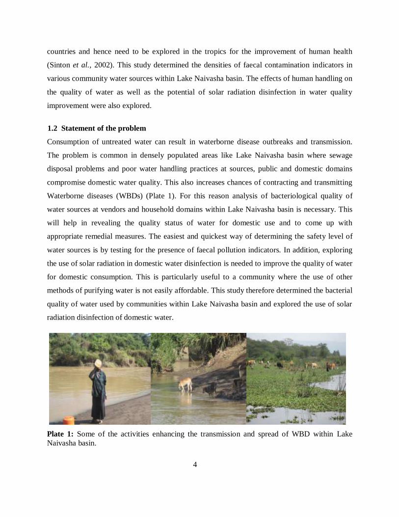
Waterborne diseases (WBDs) (Plate 1). For this reason analysis of bacteriological quality of
water sources at vendors and household domains within Lake Naivasha basin is necessary. This
will help in revealing the quality status of water for domestic use and to come up with
appropriate remedial measures. The easiest and quickest way of determining the safety level of
water sources is by testing for the presence of faecal pollution indicators. In addition, exploring
the use of solar radiation in domestic water disinfection is needed to improve the quality of water
for domestic consumption. This is particularly useful to a community where the use of other
methods of purifying water is not easily affordable. This study therefore determined the bacterial
quality of water used by communities within Lake Naivasha basin and explored the use of solar
radiation disinfection of domestic water.
Plate 1: Some of the activities enhancing the transmission and spread of WBD within Lake
Naivasha basin.
5
1.3 Objectives
1.3.1 Broad objective
To determine the bacteriological quality of water utilized by communities living in Lake
Naivasha basin and explore the use of solar radiation in domestic water disinfection.
1.3.2 Specific objectives
These were to;
(i) Determine the spatial and temporal variations in the levels of bacterial indicators of
faecal contamination in domestic water sources within Lake Naivasha basin.
(ii) Assess the effects of human water handling on the density of indicators of faecal
contamination in water for domestic consumption within Lake Naivasha basin.
(iii)Determine the ratio of E. coli to intestinal enterococci as a method of tracking the
possible source of faecal pollution into water sources.
(iv) Determine exposure time and volume for effective eradication of E. coli and total
coliforms in water for domestic consumption through solar disinfection based on the
prevailing solar radiation conditions within Lake Naivasha basin.
1.4 Hypotheses
(i) There is no spatial and temporal variation in the levels of bacterial indicators of faecal
contamination in domestic water sources within Lake Naivasha basin.
(ii) Human water handling has no effect on the density of indicators of faecal contamination
in water for domestic consumption in Lake Naivasha basin.
(iii)The ratios of E. coli to intestinal enterococci are not within the recommended values for
microbial source tracking.
(iv) Exposure time and volume does not influence eradication of E. coli and total coliforms
in water for domestic consumption within Lake Naivasha basin based on the prevailing
solar radiation conditions.
6
1.5 Justification
The best way to prevent waterborne disease outbreak in a community is by ensuring that water
for domestic consumption is safe. To ascertain the safety of water for domestic consumption, it is
critical to periodically monitor for the presence of these pathogens from all the domestic water
sources. However, it would be a futile exercise, expensive and time consuming to check for the
presence of individual pathogens. Instead, an indicator organism from the same habitat as the
pathogen and which is easy to culture and identify is used to assay for faecal contamination of
domestic water. This will give a measure of bacteriological quality of the water sources and
provide information on the appropriate method to apply in order to maintain the safety of water
for domestic use. Solar radiation as a method of water disinfection technique is cheap and
locally available in the tropics. Therefore, there is need to know the optimum time and water
volume in which the technology is most efficient under prevailing solar radiation conditions
within Lake Naivasha basin.
7
CHAPTER TWO
LITERATURE REVIEW
2.1 Introduction to Ecosystem Health
According to Karr (1999), an environment is healthy when the supply of goods and services
required by both human and non-human residents is sustained. A healthy ecosystem may be
defined in terms of three main features: vigour (a measure of activity, metabolism or primary
productivity), resilience (the ability of a system to maintain its structure in the presence of
stress), and organization (number and diversity of interactions between components of the
systems) (Mageau et al., 1995). A healthy aquatic ecosystem can also be defined as that which is
sustainable and resilient, maintaining its ecological structure and functions overtime while
continuing to meet societal needs and expectations (Meyer, 1997). According to Maddock
(1999), ecosystem indicators include the ecological status, water quality (both physico-chemical
and biological), hydrology, geomorphology and availability of physical habitat. All these
indicators are controlled by abiotic and biotic factors. Pathogens are some of the biotic
components that affect the ecosystem health since they cause diseases to man and other animals
in the ecosystem. Improvements in drinking-water supplies, excreta disposal measures and
nutritional hygiene can reduce the transmission of many infections hence keeping the ecosystem
healthy (Oomen et al., 1990). Water quality improvement measures have not been addressed in
Lake Naivasha basin despite the high population densities, poor sanitation and incidences of
diarrheal diseases outbreaks being realised in the area (Mireri, 2005). Many studies within this
area have only focused on the fisheries ecology, hydrology and chemical water quality with less
focusing on bacteriological water quality (Haper and Mavuti, 2004).
2.2 Importance of water borne diseases
Water borne diseases are mainly microbial infections which generally arise from contamination
of water by human or animal faeces or urine infested by pathogenic microbes and directly
transmitted when unsafe water is drunk or used in food preparation (WHO, 2002). Like any other
disease, WBDs also have a negative effect on the economic development, for example in 1993
cryptosporidiosis outbreak in Milwaukee (USA) made 403,000 Milwaukee residents developed
diarrhoea reflecting an attack rate of 52% of the population (Wilconsin, 1993). Over 4,000
residents were hospitalized with cryptosporidiosis which was listed as the underlying cause of
8
death in 100 patients. This lowered the economic development by making 725,000 productive
days to be lost costing $54 million in lost time and associated expenses for the Milwaukee
community (Meinhardt, 2009). These incidences of economic and life losses are also occurring
in developing countries and various measures need to be put in place to enhance water quality
improvement. Integrated Water Resource Management (IWRM) is one of such measures where
various dimension are put into consideration. Despite the effect of WBD outbreak on the
economy, safe and clean drinking water has not been a subject of interest within Naivasha flower
farm region exposing the entire population to incidences of waterborne diseases (M’cLeen,
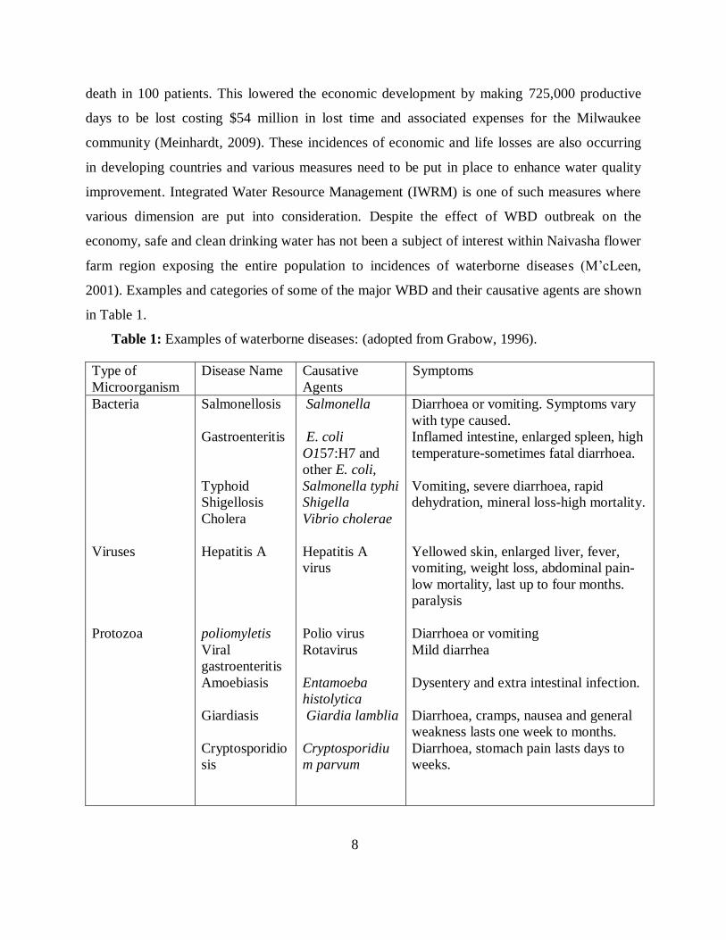
2001). Examples and categories of some of the major WBD and their causative agents are shown
in Table 1.
Table 1: Examples of waterborne diseases: (adopted from Grabow, 1996).
Type of
Microorganism
Disease Name Causative
Agents
Symptoms
Bacteria
Viruses
Protozoa
Salmonellosis
Gastroenteritis
Typhoid
Shigellosis
Cholera
Hepatitis A
poliomyletis
Viral
gastroenteritis
Amoebiasis
Giardiasis
Cryptosporidio
sis
Salmonella
E. coli
O157:H7 and
other E. coli,
Salmonella typhi
Shigella
Vibrio cholerae
Hepatitis A
virus
Polio virus
Rotavirus
Entamoeba
histolytica
Giardia lamblia
Cryptosporidiu
m parvum
Diarrhoea or vomiting. Symptoms vary
with type caused.
Inflamed intestine, enlarged spleen, high
temperature-sometimes fatal diarrhoea.
Vomiting, severe diarrhoea, rapid
dehydration, mineral loss-high mortality.
Yellowed skin, enlarged liver, fever,
vomiting, weight loss, abdominal pain-
low mortality, last up to four months.
paralysis
Diarrhoea or vomiting
Mild diarrhea
Dysentery and extra intestinal infection.
Diarrhoea, cramps, nausea and general
weakness lasts one week to months.
Diarrhoea, stomach pain lasts days to
weeks.
9
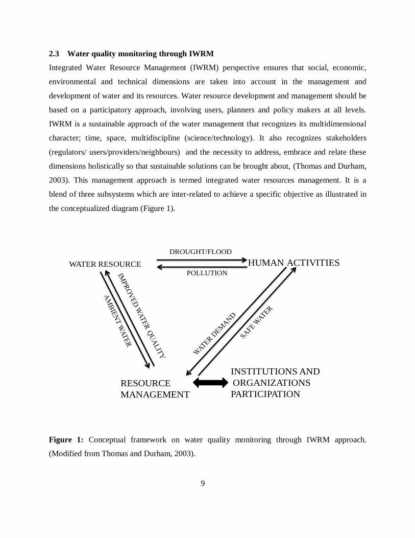
2.3 Water quality monitoring through IWRM
Integrated Water Resource Management (IWRM) perspective ensures that social, economic,
environmental and technical dimensions are taken into account in the management and
development of water and its resources. Water resource development and management should be
based on a participatory approach, involving users, planners and policy makers at all levels.
IWRM is a sustainable approach of the water management that recognizes its multidimensional
character; time, space, multidiscipline (science/technology). It also recognizes stakeholders
(regulators/ users/providers/neighbours) and the necessity to address, embrace and relate these
dimensions holistically so that sustainable solutions can be brought about, (Thomas and Durham,
2003). This management approach is termed integrated water resources management. It is a
blend of three subsystems which are inter-related to achieve a specific objective as illustrated in
the conceptualized diagram (Figure 1).
WATER RESOURCE HUMAN ACTIVITIES
RESOURCE
MANAGEMENT
INSTITUTIONS AND
ORGANIZATIONS
PARTICIPATION
DROUGHT/FLOOD
POLLUTION
Figure 1: Conceptual framework on water quality monitoring through IWRM approach.
(Modified from Thomas and Durham, 2003).
10
2.4 Sources and routes of water contamination
Many pathogenic bacteria (Clostridium botulinum type E, pathogenic Vibrio sp. and Aeromonas)
are naturally present in aquatic environments, while others (C. botulinum type A and B and
Listeria monocytogenes) occur in the general environment. Others (Salmonella spp., Shigella
spp., E.coli and enteric viruses and other protozoans and helminthes) are of animal/human origin
(Huss et al., 2000). Thus, there is often a possible likelihood that these microorganisms are
passed to the consumers when untreated water is consumed or even to the food during
production and processing if the water used is untreated. Insects, birds and rodents have been
recognized as important carriers of pathogens and other micro-organisms, (Olsen and Hammack,
2000; Urban and Broce, 2000). In one interesting case Salmonella outbreak was traced back to
amphibians, which had accidentally entered the production facility (Parish, 1998). Fenlon (1983)
and Beveridge (1988) demonstrated that some aquatic birds spread Salmonella and other human
pathogens in the environment indicating potential danger in consumption of untreated water.
Water, like food, is a vehicle for the transmission of many agents of diseases and continues to
cause significant outbreaks of diseases in developed and developing countries world-wide (Kirby
et al., 2003). In Canada, an outbreak of E. coli was reported in the year 2000 (Kondro, 2000). In
the USA Cryptosporidium affected approximately 400,000 consumers and caused 45 deaths in
1993 due to consumption of contaminated water (Kramer et al., 1996; Hoxie et al., 1997). A
cholera epidemic in Jerusalem, Israel in 1970 was traced back to the consumption of salad
vegetables irrigated with raw wastewater (Shuval et al., 1996). It is therefore important that safe
water is used throughout the production process. There should also be a monitoring program
starting from the water source, through treatment, distribution and storage within the plants and
at the vendors and household domains, to ensure that the water complies with internal or
legislative standards (Kirby et al., 2003).
2.5 Bacterial indicators of faecal pollution
Various bacteria are natural inhabitants of the digestive tracts of animals and humans and pass
into water through faeces. Some of these bacteria, such as coliforms, E. coli and Enterococcus
spp., are used as hygiene indicators (Frahm et al., 2003). Faecal contamination indicator
microorganism’s numbers points to inadequate safety in the environment as their presence in
11
aquatic systems indicate presence of faecal and sewage pollution (Mossel et al., 1995). They are
also used to assess food safety and water sanitation (Jay, 1992). There is no universal agreement
on which indicator microorganism(s) is most useful, nor are there state regulations mandating a
single standard for bacterial indicators. Thus, different indicators and different indicator levels
identified as standards are used in different states, countries, and regions. Today, the most
commonly measured bacterial indicators of faecal pollution into water sources are total coliforms
(TC), faecal coliforms (FC), (EC) E. coli (a subset of the FC group) and because their presence
in water is an indication of recent faecal pollution entrococci (Noble et al., 2003). Other bacterial
indicators can survive and proliferate in the environment and their presence may not necessarily
indicate recent faecal pollution. Owing to issues relating to complexity, cost and timeliness of
obtaining results, testing for specific pathogens is generally limited to validation, where
monitoring is used to determine whether a treatment or other process is effective in removing
target organisms (Pote et al., 2009). However, microbial testing included as part of operational
monitoring is normally limited to that for indicator organisms, either to measure the effectiveness
of control measures or as an index of faecal pollution (Jay, 1992). The concept of using indicator
organisms as signals of faecal pollution is a well-established practice in the assessment of
drinking-water quality (Noble et al., 2003). The criteria determined for such indicators and index
organisms are many. They include; the organisms to be used as indicators should not to be
pathogens themselves, they should be universally present in faeces of humans and animals in
large numbers and not multiply in natural waters, they should persist in water in a similar manner
to faecal pathogens, they should also be present in higher numbers than faecal pathogens, they
should respond to treatment processes in a similar fashion to faecal pathogens and should be
readily detected by simple inexpensive methods (Ashbolt et al., 2001).
2.5.1 Coliform bacteria
Total coliform bacteria include a wide range of aerobic and facultatively anaerobic, Gram-
negative, non-spore-forming bacilli. They are capable of growing in the presence of relatively
high concentrations of bile salts with the fermentation of lactose and production of acid or
aldehyde within 24-48 hours at 35–37 0C (APHA 2005). E. coli and thermotolerant coliforms are
a subset of the total coliform group that can ferment lactose at higher temperatures, (Bonde,
1997). As part of lactose fermentation, total coliforms produce the enzyme β-galactosidase.
12
Traditionally, coliform bacteria are regarded as belonging to the genera Escherichia, Citrobacter,
Klebsiella and Enterobacter, but the group is more heterogeneous and includes a wider range of
genera, such as Serratia and Hafnia (Doyle and Erickson, 2006). The total coliform group
includes both faecal and other environmental species. Total coliforms include organisms that can
survive and grow in water and vegetation. Hence, they are not useful as an index of faecal
pathogens, but they can be used as an indicator of treatment effectiveness and to assess the
cleanliness and integrity of distribution systems and the potential presence of biofilms, (Sueiro,
2001). Total coliform bacteria occur in both sewage and natural waters. Some of these bacteria
are excreted in the faeces of humans and animals, but many coliforms are heterotrophic and able
to multiply in water and soil environments. Total coliforms can also survive and grow in water
distribution systems, particularly in the presence of biofilms. Their presence in distribution
systems and stored water supplies can reveal regrowth and possible biofilm formation as noticed
in water storage containers. Their presence also shows contamination through increase of foreign
material, including soil or plants (Grabow, 1996, Ashbolt et al., 2001, Sueiro, 2001).
2.5.2 Thermotolerant coliform bacteria and Escherichia coli
Coliform bacteria that are able to ferment lactose at 44–450C are known as thermotolerant
coliforms. In most waters, the predominant genus of coliform bacteria is Escherichia, but some
types of Citrobacter, Klebsiella and Enterobacter are also thermotolerant. E. coli can be
differentiated from the other thermotolerant coliforms by the ability to produce indole from
tryptophan or by the production of the enzyme β-glucuronidase. E. coli is present in very high
numbers in human and animal faeces and is rarely found in the absence of faecal pollution,
although there is some evidence for growth in tropical soils (Ashbolt et al., 2001). E. coli are
considered the most suitable index of faecal contamination. In most circumstances, populations
of thermotolerant coliforms are composed predominantly of E. coli and are acceptable indicator
of faecal pollution (Sueiro, 2001). E. coli (or alternatively, thermotolerant coliforms) is the first
organism of choice in monitoring programmes for verification, including surveillance of
drinking-water quality. E. coli occur in high densities in human and animal faeces (109 per gram
of faeces), sewage and water subject to recent faecal pollution (George, 2001). This is because
water temperatures and nutrient conditions present in drinking-water distribution systems are
highly unlikely to support the growth of these organisms. The presence of E. coli provides
13
evidence of recent faecal contamination, and detection should lead to consideration of further
action, which could include further sampling and investigation of potential sources such as
inadequate treatment or breaches in distribution system integrity, (Grabow, 1996; Ashbolt et al.,
2001; George, 2001and Sueiro, 2001).
2.5.3 Clostridium perfringens
Clostridium spp. is Gram-positive, anaerobic, sulphite-reducing bacilli (Araujo, 2001; APHA,
2005). They produce spores that are exceptionally resistant to unfavourable conditions in water
environments, including UV irradiation, temperature and pH extremes, and disinfection
processes, such as chlorination (Ashbolt et al., 2001). The characteristic species of the genus, C.
perfringens, is a member of the normal intestinal flora of 13–35% of humans and other warm-
blooded animals. Other species are not exclusively of faecal origin. Unlike E. coli, C.
perfringens does not multiply in most water environments and is a highly specific indicator of
faecal pollution. In view of the exceptional resistance of C. perfringens spores to disinfection
processes and other unfavourable environmental conditions, it has been proposed as an indicator
of enteric viruses and protozoa in treated drinking water supplies (Njeminski et al., 2000).
In addition, C. perfringens can serve as an index of faecal pollution that took place recently and
hence indicate sources liable to intermittent contamination (Araujo, 2001, Ashbolt et al., 2001).
C. perfringens is not recommended for routine monitoring, since the exceptionally long survival
times of its spores are likely to exceed those of enteric pathogens, including viruses and
protozoa. C. perfringens spores are smaller than protozoan (oo)cysts and may be useful
indicators of the effectiveness of filtration processes (Njeminski et al., 2000). Low numbers in
some source waters suggest that use of C. perfringens spores for this purpose may be limited to
validation of processes rather than routine monitoring. C. perfringens and its spores are virtually
always present in sewage and they do not multiply in clean water environments. They are more
often present in higher numbers in the faeces of some animals, such as dogs, than in the faeces of
humans and many other warm-blooded animals (Araujo, 2001, Ashbolt et al., 2001). The
numbers excreted in faeces are normally substantially lower than those of E. coli. Vegetative
cells and spores of C. perfringens are usually detected by MFT in which membranes are
incubated on selective media under strict anaerobic conditions (APHA 2005). Filtration
14
processes designed to remove enteric viruses or protozoa should also remove C. perfringens.
Detection in water immediately after treatment should lead to investigation of the filtration plant
performance, (Njeminski et al., 2000).
2.5.4 Enterococci as indicators of faecal pollution
Enterococci is a sub group of faecal streptococci and differentiated from other streptococci by
their ability to grow in 6.5% sodium chloride at pH 9.6 and 100C -45
0C. It is a valuable bacterial
indicator for determining the extent of faecal contamination in aquatic systems (APHA 2005).
Presence of faecal enterococci when E. coli is not detected is an indicator that there is recent
faecal pollution in water.
2.5.5 Heterotrophic plate count
The numbers of colony forming units of heterotrophic bacteria in water are indicators of
pollution with easily degradable organic matter. HPC also known as the standard plate count is a
procedure for estimating the number of live heterotrophic bacteria in water and measuring
changes during water treatment, distribution or in swimming pools. Colonies may arise from
pairs, chains, clusters or single cells, all called colony forming units. The final count also
depends on the interaction among the developing colonies, (APHA, 2005). In surface water they
are an indication that water is loaded with high concentration of assimilable organic carbon
(AOC) as it is normally the case with domestic sewage pollution. High densities of HPCs in
water may indicate high oxygen consumption, high heterotrophic activity, high BOD and low
DO (APHA, 2005).
2.6 Bacteriological water quality analyses methods
2.6.1 Membrane filtration technique
In the membrane filter method, membranes with a pore size that will retain bacteria but allow
water or diluents to pass through are used. Following the collection of bacteria upon filtering a
given volume, the membrane is placed on an agar plate or an absorbent pad saturated with
culture medium of choice, and incubated appropriately and after growth, colonies are enumerated
(Jay, 1992; APHA, 2005). This method offers rapid quantitative enumeration and more efficient
than other methods. This is because it is able to work with flexible sample volume range
enabling the use of large sample volume and increasing sensitivity. Water soluble impurities
15
interfering with the growth of target organisms are separated from the sample in the filtration
step. It also gives quantitative result and good precision if the number of colonies grows
adequately and further cultivation steps are not always needed. This lowers the costs and time
needed for the analysis. When confirmation is needed, isolation from well separated colonies on
membrane is easy. On the other hand it causes some difficulties as; quality of membranes varies,
solid particles and chemicals adsorbed from sample to the membrane during filtration may
interfere with the growth of the target organism, not applicable to turbid samples and scoring of
typical colonies not always easy (APHA, 2005).
Total coliforms are generally measured in 100 ml samples of water. A variety of relatively
simple procedures are available based on the production of acid from lactose or the production of
the enzyme β-galactosidase. The procedures include membrane filtration followed by incubation
of the membranes on selective media at 35-37 0C and counting of colonies after 24 hours.
Alternative methods include most probable number procedures using tubes or micro-titre plates
and presence/absence (P/A) tests. Total coliforms should be absent immediately after
disinfection, and the presence of these organisms indicates inadequate treatment. E. coli is also
generally measured in 100 ml samples of water. A variety of relatively simple procedures are
available based on the production of acid and gas from lactose or the production of the enzyme
β-glucuronidase. The procedures include membrane filtration followed by incubation of the
membranes on selective media at 44-45 0C and counting of colonies after 24 hours. Alternative
methods include most probable number procedures using tubes or micro-titre plates and P/A
tests, some for volumes of water larger than 100 ml (APHA, 2005). According to WHO
guidelines, risk assessment is based on the levels of E. coli, i.e. low, moderate, high and very
high risks of water borne disease infection as indicated by the following respective numbers of E.
coli per 10 ml of water i.e. <1, 1-9, 1-10 and > 10 respectively (WHO, 2002).
2.6.2 Most probable number
The most probable number method consists of inoculating a series of tubes with appropriate
decimal dilutions of the sample. Production of gas, acid formation or abundant growth in the test
tube after a certain period of time incubation at 35 0C constitutes a positive presumptive reaction.
Both lactose and Laury Tryptose broths can be used as presumptive media. All tubes with

16
positive presumptive reaction are subsequently subjected to a confirmation test. The formation of
gas in a Brilliant Green Lactose Bile (BGLB) broth fermentation tube at any time within 48
hours at 35 0C constitutes a positive confirmation test. A test using an EC medium can be applied
to determine TC that are FC, the production of gas after 24 hours of incubation at 44.5 0C in an
EC broth medium is considered a positive result (Rompré et al., 2002).
2.6.3 Flow cytometry
This is a technology in which a variety of measurements can be made on particles, cells, bacteria
and other objects suspended in a liquid. In a flow cytometer, particles are made to flow one at a
time through a light beam (laser beam) in a sensing region of a flow chamber. They are
characterised by light scattering based on their size, shape and density. This also depend on the
dyes that are used either independently or bound to specific antibodies or oligonucleotides that
endow a fluorescent phenotype onto components of interest. As a particle flows through the
beam, both light scattered by the particle and fluorescence light from the labelled particle is
collected. This is done either by a photomultiplier or photodiode in combination with light
splitters (dicroic mirrors) and filters (Vesey et al., 1994). A solid phase laser scanning analyzer
might be an alternative for the flow cytometry technology (Deere et al., 2002). The basic
instrument is the flow cytometer, which is expensive and requires a skilled operator. In addition,
most of the pathogenic microbes to be measured occur in drinking water at very low
concentrations. When a negative sample is analyzed no particles should be detected and a sample
seeded with an aliquot of organisms should have an exact number of particles added (Vesey et
al., 1994).
2.7 Effects of human handling practices on the quality of water
Faecal contamination of domestic water sources due to activities like improper waste discharge
and low sanitation standards within the households renders the water unsafe for domestic usage
in developing countries. Majority of people in these countries lack access to piped water and
therefore are forced to transport and store the water in their house holds for varied period of time
depending on the frequency of use during which the quality may be compromised (Wright et al.,
2004). There are two major contamination domains in water supply; public and
household/domestic domain which should frequently be monitored to ensure that the quality
17
from source is maintained at domestic level. This is because if the levels of contamination at the
public domains are high, then efforts at domestic domain may be futile (Jensen et al., 2002).
Contamination at times enhanced by presence of vendors in the water distribution chain (Kjellen
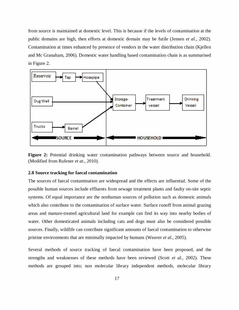
and Mc Granaham, 2006). Domestic water handling based contamination chain is as summarised
in Figure 2.
Figure 2: Potential drinking water contamination pathways between source and household.
(Modified from Rufener et at., 2010).
2.8 Source tracking for faecal contamination
The sources of faecal contamination are widespread and the effects are influential. Some of the
possible human sources include effluents from sewage treatment plants and faulty on-site septic
systems. Of equal importance are the nonhuman sources of pollution such as domestic animals
which also contribute to the contamination of surface water. Surface runoff from animal grazing
areas and manure-treated agricultural land for example can find its way into nearby bodies of
water. Other domesticated animals including cats and dogs must also be considered possible
sources. Finally, wildlife can contribute significant amounts of faecal contamination to otherwise
pristine environments that are minimally impacted by humans (Weaver et al., 2005).
Several methods of source tracking of faecal contamination have been proposed, and the
strengths and weaknesses of these methods have been reviewed (Scott et al., 2002). These
methods are grouped into; non molecular library independent methods, molecular library

18
dependent methods, molecular library independent methods and chemical methods. Non
molecular library independent methods include the use of faecal bacterial ratios and non-
molecular host specific indicators. Molecular library dependent methods are repetitive
polymerase chain reaction, pulse field gel electrophoresis, ribotyping and randomly amplified
polymorphic DNA. Molecular library independent methods are bacteriophage indicators and
virus (human pathogen) indicators (Simpson et al., 2002).
Faecal bacterial ratios is one of the techniques developed in the source tracking field and is
mainly based on the ratios of faecal coliform (E. coli) to fecal streptococci (intestinal
enterococci) (FC:FS). In this method CFUs (Colony Forming Units) of faecal coliforms and
faecal streptococci are counted on plates and a ratio between the two is determined. A ratio of
more than 4 is considered human contamination and a ratio of less than 0.7 suggests non-human
sources. Die-off rates are monitored through time and the change in the FC:FS ratio is then used
to further interpret possible sources. FC:FS ratios is still useful as a general indicator of human
verses non-human faecal bacterial contamination (Weaver et al., 2005).
2.9 Solar pasteurization
Microorganisms are heat sensitive and require temperatures of between 50-75 0C for 99.9%
elimination (Negar and Metcalf, 1999). The most favourable region for solar disinfection lies
between latitudes 150 N/S and 35
0 North and South of the Equator. These semi-arid regions are
characterised by high solar radiation (3000 hours sunshine per year) and limited cloud coverage
and rainfall. The second most favourable region lies between the equator and latitude 150 North
and South of the Equator, the scattered radiation in this region is quite high (2500 hours sunshine
per year). The need for a low-cost, low maintenance and effective disinfection system for
providing safe drinking water is paramount, especially for the developing countries. Previous
studies had also found that river water in 4 litres cooking pots could be heated to 80 0C or more
in 2 hours in a Solar Box Cooker (SBC), killing all coliform and faecal coliform bacteria
(Metcalf and Logvin 1999). Metcalf and Logvin (1999) explored the use of an SBC and built one
which was deep enough to hold three to four 3.7-liter (1-gallon) jugs and investigated what
temperatures would be reached in 1, 2, and 3 jugs of water in SBC at various times of the year
and under different weather conditions. They also investigated what time-volume combinations

19
would be sufficient to kill coliform bacteria in river water and used the heat inactivation of
coliforms as an index of water pasteurization. It has also been found that heating water to a
temperature of 65 0C with no specific time duration and volume will pasteurize water and make
it safe for drinking (Robert, 2005).

20
CHAPTER THREE
MATERIALS AND METHODS
3.1 Study area
3.1.1 Geographical location
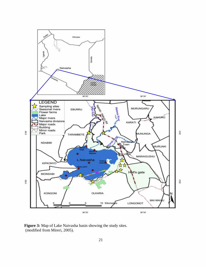
This study was carried out in Lake Naivasha basin (Fig. 3) within Africa. The basin is in Rift
Valley Province of Kenya. The lake is one of the major water bodies in Kenya besides Lake
Victoria, Lake Turkana, Lake Baringo, lake Bogoria, and Lake Elementaita. Lake Naivasha is a
fresh water lake though it lacks a well established outlet. It is located within the Kenyan Rift
Valley and its watershed covers parts of both, the Rift Valley and the Central Provinces. Lake
Naivasha watershed is mainly a semi-arid environment with scarce surface and underground
water resources. The lake basin extends 60 North from the Equator and lies between 36
007′ and
36047′ East of Greenwich Meridian.
3.1.2 Rainfall and temperature patterns
Lake Naivasha is located in the rain shadow of the Aberdare Range with a mean annual rainfall
of about 650 millimetres and experiences long rains in months of March to May and short rain in
the months of September to October. The mean annual rainfall in Lake Naivasha area as well as
in the Aberdare Range is 1350 millimetres. The mean temperature around Lake Naivasha is
approximately 25 0C with a maximum temperature of 30
0C, with the months of December –
March being the hottest period. July is the coldest month with a mean temperature of 23 0C.
(Mireri, 2005).
3.1.3 Water sources
The Lake Naivasha watershed is mainly drained by only two perennial rivers, namely Malewa
and Gilgil with catchment areas of 1700 km2 and 400 km
2 respectively. These two rivers drain
into the lake at its Northern side. In addition, the lake is also drained by other seasonal rivers and
streams with the major one being River Karati to the North. The lake, rivers, shallow wells and
ground water sources are key to sources of water to the Naivasha and Nakuru municipalities as
well as other adjoining human activities (Mireri, 2005).
21
Figure 3: Map of Lake Naivasha basin showing the study sites.
(modified from Mireri, 2005).
22
3.2 Study design
3.2.1 Sampling
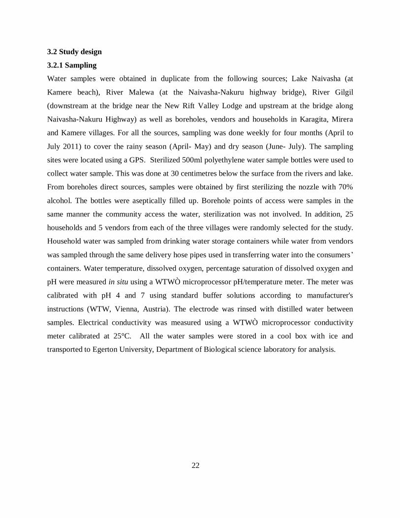
Water samples were obtained in duplicate from the following sources; Lake Naivasha (at
Kamere beach), River Malewa (at the Naivasha-Nakuru highway bridge), River Gilgil
(downstream at the bridge near the New Rift Valley Lodge and upstream at the bridge along
Naivasha-Nakuru Highway) as well as boreholes, vendors and households in Karagita, Mirera
and Kamere villages. For all the sources, sampling was done weekly for four months (April to
July 2011) to cover the rainy season (April- May) and dry season (June- July). The sampling
sites were located using a GPS. Sterilized 500ml polyethylene water sample bottles were used to
collect water sample. This was done at 30 centimetres below the surface from the rivers and lake.
From boreholes direct sources, samples were obtained by first sterilizing the nozzle with 70%
alcohol. The bottles were aseptically filled up. Borehole points of access were samples in the
same manner the community access the water, sterilization was not involved. In addition, 25
households and 5 vendors from each of the three villages were randomly selected for the study.
Household water was sampled from drinking water storage containers while water from vendors
was sampled through the same delivery hose pipes used in transferring water into the consumers’
containers. Water temperature, dissolved oxygen, percentage saturation of dissolved oxygen and
pH were measured in situ using a WTWÒ microprocessor pH/temperature meter. The meter was
calibrated with pH 4 and 7 using standard buffer solutions according to manufacturer's
instructions (WTW, Vienna, Austria). The electrode was rinsed with distilled water between
samples. Electrical conductivity was measured using a WTWÒ microprocessor conductivity
meter calibrated at 25°C. All the water samples were stored in a cool box with ice and
transported to Egerton University, Department of Biological science laboratory for analysis.

23
3.2.2 Description of sampling sites and water sources
The location and categories of water sources sampled were as described in Table 2.
Table 2: Description and location of study sites
CODE FULL NAME OF THE SOURCES LOCATION
KRBHI -DIR Karagita borehole I-direct source S000,46',48.8''/E036
0,26',17.7''
KRBHI -POA Karagita borehole I-point of access S000,46',48.8''/E036
0,26',17.7''
KRBHII- POA Karagita borehole II-point of Access S000,46',40.4''/E036
0,26',09.2''
KRBHIII -DR Karagita borehole III-direct source S000,46',29.7''/E036
0,26',10.7''
KRBHIII-POA Karagita borehole III-point of Access S000,46',36.5''/E036
0,26',07.5''
KRBHIV-DIR Karagita borehole IV direct source S000,46',50.2''/E036
0,26',01.4''
KRBHV-POA Karagita borehole V point of Access S000,46',42.8''/ E036
0,25',43.1''
DCK-DIR DCK direct source S000,49',59.1''/E036
0,20',57.8''
KMBEACH Kamere beach S000,48',53.2''/ E036
0,19',28.4''
MAL RVR River Malewa S000,40.0',8.8''/E036
0,23.0',18.7''
GL RVR-UP River Gilgil upstream S000,33.0',38.8''/E036
0,21.0',28.0''
GL RVR-DWN River Gilgil downstream S000,32.0',18.8''/E036
0,23.0',12.6''
(i) Borehole water - Direct (DIR) Sources
For direct borehole waters, samples were obtained directly from the boreholes as it was being
pumped. This involved opening of the metal pipes from the valves/points where they are joined
using an adjustable spanner. The pipe was sterilized with ethanol before the samples were
obtained.
Plate 2: Direct borehole sites; (a) DCK and (b) KRBH III
(a) (b)
24
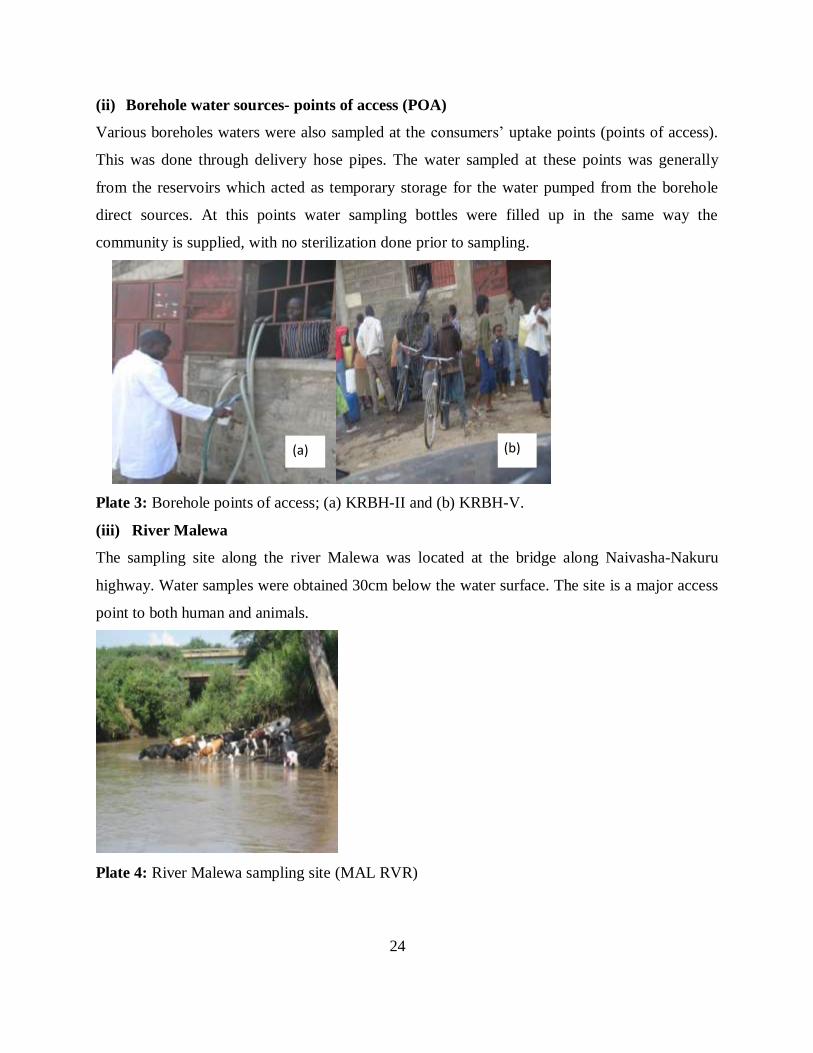
(ii) Borehole water sources- points of access (POA)
Various boreholes waters were also sampled at the consumers’ uptake points (points of access).
This was done through delivery hose pipes. The water sampled at these points was generally
from the reservoirs which acted as temporary storage for the water pumped from the borehole
direct sources. At this points water sampling bottles were filled up in the same way the
community is supplied, with no sterilization done prior to sampling.
Plate 3: Borehole points of access; (a) KRBH-II and (b) KRBH-V.
(iii) River Malewa
The sampling site along the river Malewa was located at the bridge along Naivasha-Nakuru
highway. Water samples were obtained 30cm below the water surface. The site is a major access
point to both human and animals.
Plate 4: River Malewa sampling site (MAL RVR)
(a) (b)

25
(iv) River Gilgil
Two sites were sampled along River Gilgil; downstream site at the bridge along Morendat
Training and Conference Centre towards the new Rift Valley Lodge road and the up-stream site
at the bridge along Naivasha- Nakuru highway. The upstream site was noted to be the major
access point for both animals and man.
Plate 5: River Gilgil sampling sites.
(a) Upstream (GL RVR-UP) (b) downstream (GL RVR-DWN).
(v) Kamere Beach
This site was at the northern side of Lake Naivasha. It is the main access point to the lake and
was noted to be harbouring several activities ranging from laundry work, fish landing, watering
and grazing of both domestic and wild animals as well as washing of tracks. Water for domestic
use was also being obtained from the same point by some vendors and households.
Plate 6: Sampling site within Lake Naivasha at Kamere Beach (KMBEACH)
(b)
(a) (b)
26
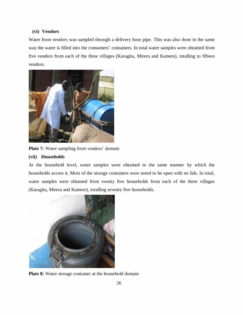
(vi) Vendors
Water from vendors was sampled through a delivery hose pipe. This was also done in the same
way the water is filled into the consumers’ containers. In total water samples were obtained from
five vendors from each of the three villages (Karagita, Mirera and Kamere), totalling to fifteen
vendors.
Plate 7: Water sampling from vendors’ domain
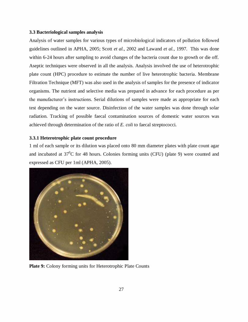
(vii) Households
At the household level, water samples were obtained in the same manner by which the
households access it. Most of the storage containers were noted to be open with no lids. In total,
water samples were obtained from twenty five households from each of the three villages
(Karagita, Mirera and Kamere), totalling seventy five households.
Plate 8: Water storage container at the household domain
27
3.3 Bacteriological samples analysis
Analysis of water samples for various types of microbiological indicators of pollution followed
guidelines outlined in APHA, 2005; Scott et al., 2002 and Lawand et al., 1997. This was done
within 6-24 hours after sampling to avoid changes of the bacteria count due to growth or die off.
Aseptic techniques were observed in all the analysis. Analysis involved the use of heterotrophic
plate count (HPC) procedure to estimate the number of live heterotrophic bacteria. Membrane
Filtration Technique (MFT) was also used in the analysis of samples for the presence of indicator
organisms. The nutrient and selective media was prepared in advance for each procedure as per
the manufacturer’s instructions. Serial dilutions of samples were made as appropriate for each
test depending on the water source. Disinfection of the water samples was done through solar
radiation. Tracking of possible faecal contamination sources of domestic water sources was
achieved through determination of the ratio of E. coli to faecal streptococci.
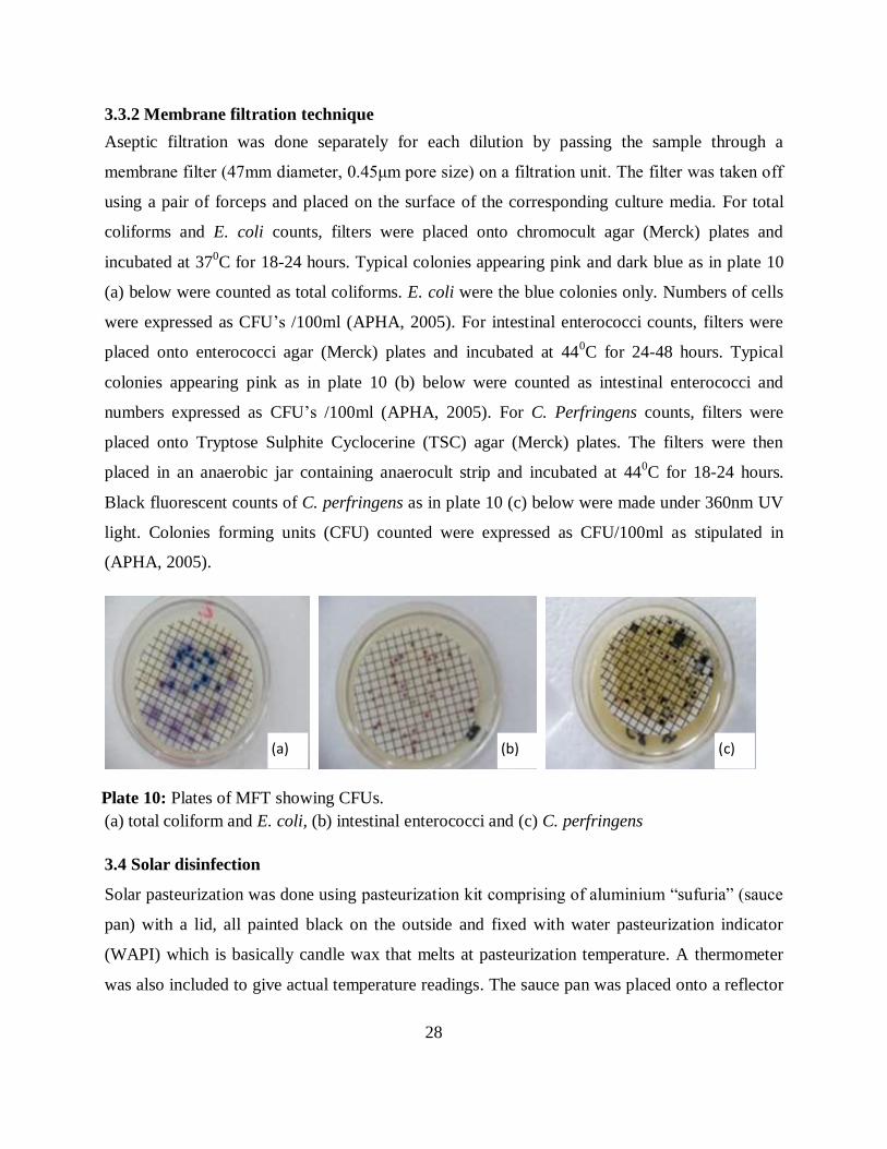
3.3.1 Heterotrophic plate count procedure
1 ml of each sample or its dilution was placed onto 80 mm diameter plates with plate count agar
and incubated at 370C for 48 hours. Colonies forming units (CFU) (plate 9) were counted and
expressed as CFU per 1ml (APHA, 2005).
Plate 9: Colony forming units for Heterotrophic Plate Counts
28
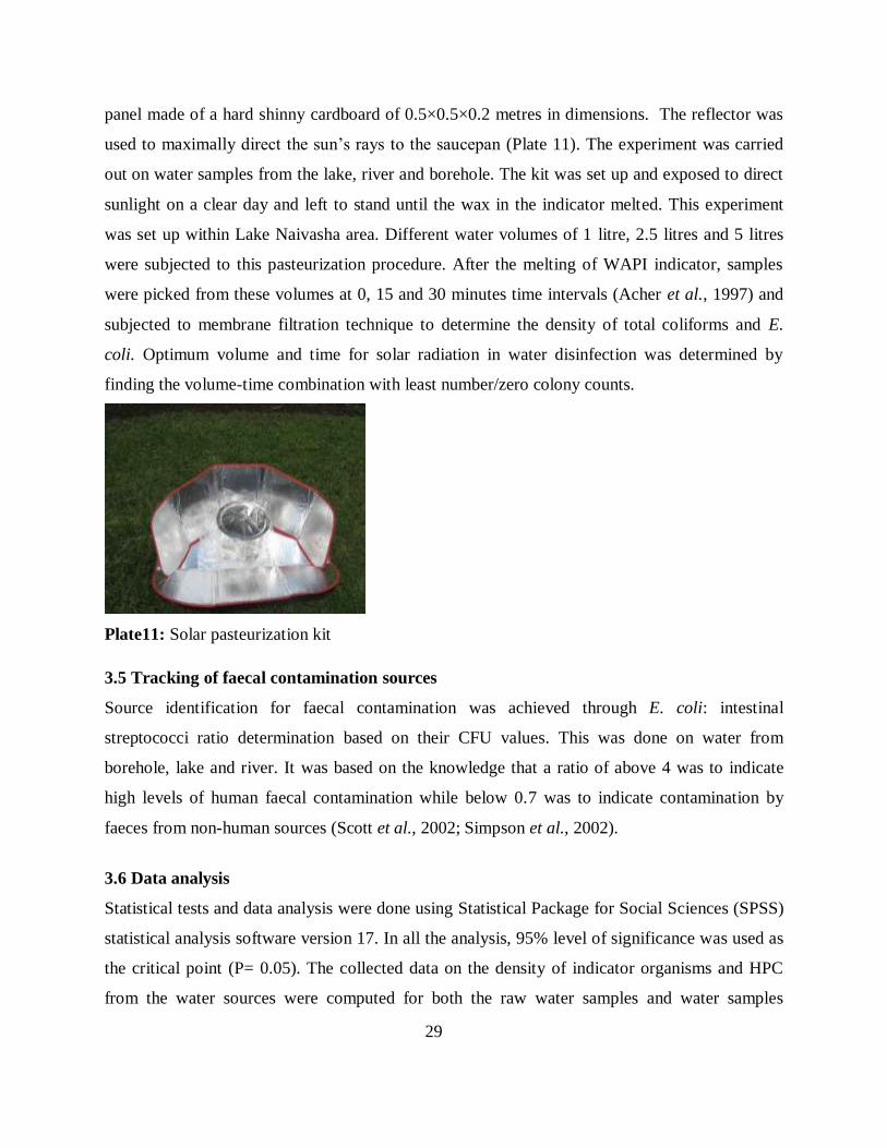
3.3.2 Membrane filtration technique
Aseptic filtration was done separately for each dilution by passing the sample through a
membrane filter (47mm diameter, 0.45μm pore size) on a filtration unit. The filter was taken off
using a pair of forceps and placed on the surface of the corresponding culture media. For total
coliforms and E. coli counts, filters were placed onto chromocult agar (Merck) plates and
incubated at 370C for 18-24 hours. Typical colonies appearing pink and dark blue as in plate 10
(a) below were counted as total coliforms. E. coli were the blue colonies only. Numbers of cells
were expressed as CFU’s /100ml (APHA, 2005). For intestinal enterococci counts, filters were
placed onto enterococci agar (Merck) plates and incubated at 440C for 24-48 hours. Typical
colonies appearing pink as in plate 10 (b) below were counted as intestinal enterococci and
numbers expressed as CFU’s /100ml (APHA, 2005). For C. Perfringens counts, filters were
placed onto Tryptose Sulphite Cyclocerine (TSC) agar (Merck) plates. The filters were then
placed in an anaerobic jar containing anaerocult strip and incubated at 440C for 18-24 hours.
Black fluorescent counts of C. perfringens as in plate 10 (c) below were made under 360nm UV
light. Colonies forming units (CFU) counted were expressed as CFU/100ml as stipulated in
(APHA, 2005).
Plate 10: Plates of MFT showing CFUs.
(a) total coliform and E. coli, (b) intestinal enterococci and (c) C. perfringens
3.4 Solar disinfection
Solar pasteurization was done using pasteurization kit comprising of aluminium “sufuria” (sauce
pan) with a lid, all painted black on the outside and fixed with water pasteurization indicator
(WAPI) which is basically candle wax that melts at pasteurization temperature. A thermometer
was also included to give actual temperature readings. The sauce pan was placed onto a reflector
(a) (b) (c)
29
panel made of a hard shinny cardboard of 0.5×0.5×0.2 metres in dimensions. The reflector was
used to maximally direct the sun’s rays to the saucepan (Plate 11). The experiment was carried
out on water samples from the lake, river and borehole. The kit was set up and exposed to direct
sunlight on a clear day and left to stand until the wax in the indicator melted. This experiment
was set up within Lake Naivasha area. Different water volumes of 1 litre, 2.5 litres and 5 litres
were subjected to this pasteurization procedure. After the melting of WAPI indicator, samples
were picked from these volumes at 0, 15 and 30 minutes time intervals (Acher et al., 1997) and
subjected to membrane filtration technique to determine the density of total coliforms and E.
coli. Optimum volume and time for solar radiation in water disinfection was determined by
finding the volume-time combination with least number/zero colony counts.
Plate11: Solar pasteurization kit
3.5 Tracking of faecal contamination sources
Source identification for faecal contamination was achieved through E. coli: intestinal
streptococci ratio determination based on their CFU values. This was done on water from
borehole, lake and river. It was based on the knowledge that a ratio of above 4 was to indicate
high levels of human faecal contamination while below 0.7 was to indicate contamination by
faeces from non-human sources (Scott et al., 2002; Simpson et al., 2002).
3.6 Data analysis
Statistical tests and data analysis were done using Statistical Package for Social Sciences (SPSS)
statistical analysis software version 17. In all the analysis, 95% level of significance was used as
the critical point (P= 0.05). The collected data on the density of indicator organisms and HPC
from the water sources were computed for both the raw water samples and water samples
30
pasteurized at different duration of time time (0, 15 and 30 minutes) and volumes (1 , 2.5 and 5
litres) to find the mean densities from each sampling site and for each water source. Data on
physical and chemical parameters (pH, Temperature, DO and Conductivity) were also computed
for all the water sources to find the variation in mean values. One way Analysis of Variance
(ANOVA) was used to compare means recorded at different sampling dates and/or sites for
various selected variables. Student’s t-test was used to compare the means of microbiological
parameters between borehole direct sources and borehole points of access. Means were separated
using least significance difference (LSD) as the post hoc test. Correlation analysis was used to
compare relationship between the densities of microbial parameters and physico-chemical
parameters.
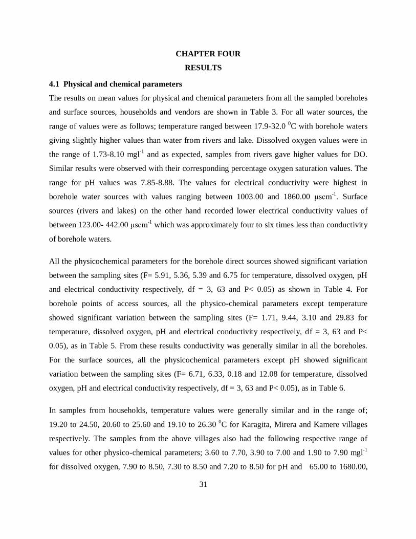
31
CHAPTER FOUR
RESULTS
4.1 Physical and chemical parameters
The results on mean values for physical and chemical parameters from all the sampled boreholes
and surface sources, households and vendors are shown in Table 3. For all water sources, the
range of values were as follows; temperature ranged between 17.9-32.0 0C with borehole waters
giving slightly higher values than water from rivers and lake. Dissolved oxygen values were in
the range of 1.73-8.10 mgl-1
and as expected, samples from rivers gave higher values for DO.
Similar results were observed with their corresponding percentage oxygen saturation values. The
range for pH values was 7.85-8.88. The values for electrical conductivity were highest in
borehole water sources with values ranging between 1003.00 and 1860.00 μscm-1
. Surface
sources (rivers and lakes) on the other hand recorded lower electrical conductivity values of
between 123.00- 442.00 μscm-1
which was approximately four to six times less than conductivity
of borehole waters.
All the physicochemical parameters for the borehole direct sources showed significant variation
between the sampling sites (F= 5.91, 5.36, 5.39 and 6.75 for temperature, dissolved oxygen, pH
and electrical conductivity respectively, df = 3, 63 and P< 0.05) as shown in Table 4. For
borehole points of access sources, all the physico-chemical parameters except temperature
showed significant variation between the sampling sites (F= 1.71, 9.44, 3.10 and 29.83 for
temperature, dissolved oxygen, pH and electrical conductivity respectively, df = 3, 63 and P<
0.05), as in Table 5. From these results conductivity was generally similar in all the boreholes.
For the surface sources, all the physicochemical parameters except pH showed significant
variation between the sampling sites (F= 6.71, 6.33, 0.18 and 12.08 for temperature, dissolved
oxygen, pH and electrical conductivity respectively, df = 3, 63 and P< 0.05), as in Table 6.
In samples from households, temperature values were generally similar and in the range of;
19.20 to 24.50, 20.60 to 25.60 and 19.10 to 26.30 0C for Karagita, Mirera and Kamere villages
respectively. The samples from the above villages also had the following respective range of
values for other physico-chemical parameters; 3.60 to 7.70, 3.90 to 7.00 and 1.90 to 7.90 mgl-1
for dissolved oxygen, 7.90 to 8.50, 7.30 to 8.50 and 7.20 to 8.50 for pH and 65.00 to 1680.00,
32
384.00 to 1232.00 and 22.00 to 1667.00 μscm-1
for electrical conductivity. Water samples from
vendors had the following range for physical and chemical parameters; 17.90 to 23.10 0C, 1.90 to
5.00 mgl-1
, 6.90 to 8.60 and 250.00 to 1435.00 μscm-1
respectively for; temperature, dissolved
oxygen, pH and electrical conductivity.
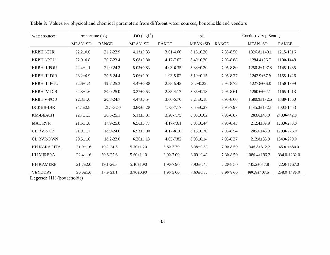
33
Table 3: Values for physical and chemical parameters from different water sources, households and vendors
Water sources Temperature (°C) DO (mgl-1
) pH
Conductivity (μScm-1
)
MEAN±SD RANGE MEAN±SD RANGE MEAN±SD RANGE MEAN±SD RANGE
KRBH I-DIR 22.2±0.6 21.2-22.9 4.13±0.33 3.61-4.60 8.16±0.20 7.85-8.50 1326.8±140.1 1215-1616
KRBH I-POU 22.0±0.8 20.7-23.4 5.68±0.80 4.17-7.62 8.40±0.30 7.95-8.88 1284.4±96.7 1190-1448
KRBH II-POU 22.4±1.1 21.0-24.2 5.03±0.83 4.03-6.35 8.38±0.20 7.95-8.80 1250.8±107.8 1145-1435
KRBH III-DIR 23.2±0.9 20.5-24.4 3.06±1.01 1.93-5.02 8.10±0.15 7.95-8.27 1242.9±87.9 1155-1426
KRBH III-POU 22.6±1.4 19.7-25.3 4.47±0.80 2.85-5.42 8.2±0.22 7.95-8.72 1227.8±86.8 1150-1399
KRBH IV-DIR 22.3±1.6 20.0-25.0 3.27±0.53 2.35-4.17 8.35±0.18 7.95-8.61 1260.6±92.1 1165-1413
KRBH V-POU 22.8±1.0 20.8-24.7 4.47±0.54 3.66-5.70 8.23±0.18 7.95-8.60 1580.9±172.6 1380-1860
DCKBH-DIR 24.4±2.8 21.1-32.0 3.80±1.20 1.73-7.17 7.50±0.27 7.95-7.97 1145.3±132.1 1003-1453
KM-BEACH 22.7±1.3 20.6-25.1 5.13±1.81 3.20-7.75 8.05±0.62 7.95-8.87 283.6±48.9 248.0-442.0
MAL RVR 21.5±1.8 17.9-25.0 6.56±0.77 4.17-7.61 8.03±0.44 7.95-8.43 212.4±39.9 123.0-273.0
GL RVR-UP 21.9±1.7 18.9-24.6 6.93±1.00 4.17-8.10 8.13±0.30 7.95-8.54 205.6±43.3 129.0-276.0
GL RVR-DWN 20.5±1.0 18.2-22.0 6.26±1.13 4.03-7.82 8.08±0.14 7.95-8.27 212.8±36.9 134.0-270.0
HH KARAGITA 21.9±1.6 19.2-24.5 5.50±1.20 3.60-7.70 8.38±0.30 7.90-8.50 1346.8±312.2 65.0-1680.0
HH MIRERA 22.4±1.6 20.6-25.6 5.60±1.10 3.90-7.00 8.00±0.40 7.30-8.50 1080.4±196.2 384.0-1232.0
HH KAMERE 21.7±2.0 19.1-26.3 5.40±1.90
1.90-7.90 7.90±0.40 7.20-8.50 735.2±617.8 22.0-1667.0
VENDORS 20.6±1.6 17.9-23.1 2.90±0.90 1.90-5.00 7.60±0.50 6.90-8.60 990.8±403.5 258.0-1435.0
Legend: HH (households)
34
Table 4: Spatial variation of physico-chemical parameters in borehole direct water sources
Water sources Temperature DO pH Conductivity
KRBH I-DIR 22.22a 4.13a 8.17a 1326.81a
KRBH III-DIR 23.23a 3.07b 8.10a 1242.88b
KRBH IV-DIR 22.36a 3.27bc 8.35b 1260.69ab
DCK-DIR 24.46b 3.80ac 8.23c 1145.31c
Legend: Means in a column followed by different letters are significantly different at p<0.05 by
LSD.
Table 5: Spatial variation of physico-chemical parameters in the borehole points of use sources
Water sources Temperature DO pH Conductivity
KRBH I-POU 22.03a 5.69a 8.41a 1284.44a
KRBH II-POU 22.49ab 5.04b 8.38ac 1250.81a
KRBH III-POU 22.68ab 4.48c 8.20b 1227.81a
KRBH V-POU 22.88b 5.01c 8.23cb 1580.94b
Legend: Means in a column followed by different letters are significantly different at p<0.05 by
LSD.
Table 6: Spatial variation of physico-chemical parameters in surface water sources
Water sources Temperature DO pH Conductivity
KAMERE 22.76a 5.13a 8.05a 283.63a
MAL-RVR 21.59bc 6.56b 8.04a 212.44b
GIL RVR-UP 21.99abd 6.94b 8.14a 205.56b
GIL RVR-DWN 20.56cd 6.26b 8.08a 212.81b
Legend: Means in a column followed by different letters are significantly different at p<0.05 by
LSD.
4.2. Microbiological parameters
4.2.1 Boreholes
4.2.1.1 Spatial variation
Results for values of microbiological parameters in water samples from borehole-direct sources
(BH-DIR) are shown in Figure 4 and Appendix 3. Lower values of the following range; 0-2.00
CFU/100 ml, 6.00-25.500 CFU/100 ml, 0-2.00 CFU/100 ml, 0-1.00 CFU/100 ml and 60.00-
460.00 CFU/100 ml were recorded for E. coli, total coliforms, intestinal enterococci, C.
perfringens and HPC respectively. From these results, samples from Denmark Company of
Kenya (DCK) borehole gave higher values for all the microbiological parameters than the other
borehole direct sources. The means for borehole direct sources (BH-DIR) had no significant
35
variation with respect to sites (F= 0.427, 0.291, 0.977, 0.124 and 0.053 for E. coli, total coliform,
intestinal enterococci, C. perfringens and HPC respectively, df= 3, 63 and P>0.05). During the
four months of the weekly sampling period 12% positive result on faecal contamination
indicators was obtained from these BH-DIR sources.
Figure 4: Densities of faecal contamination indicators in borehole direct water sources.
Results for microbiological parameters values in water samples from borehole points of access
(BH-POA) sources are given in Figure 5 and Appendix 4. For all the boreholes-point of access
sources (BH-POA), all the microbiological parameters showed significant variation with respect
to sites (F= 4.358, 13.101, 3.519, 3.165 and 6.165 for E. coli, total coliform, intestinal
enterococci, C. perfringens and HPC respectively, df= 3, 63 and P<0.05), as in Table 7. During
the four months of sampling, 39% positive result on faecal contamination indicators was
obtained from these BH-POA sources.
Legend: EC (E. coli), TC (total
coliforms), IE (intestinal enterococci),
CP (C. perfringens) and HPC
(heterotrophic Plate count), Vertical
Bars = +standard error, n=16.

36
Figure 5: Densities of indicators of faecal contamination in boreholes points of access sources.
Table 7: Spatial variation on the microbial parameters for the borehole points of access sources.
SOURCES EC TC IE CP HPC
BH I -POA 2.18a 19.31a 1.44a 0.25a 262.81a
BHII -POA 2.31a 24.22b 2.13b 1.38b 340.00b
BH III -POA 1.75a 22.13ab 0.88a 0.44a 324.69a
BH V -POA 2.63b 23.97b 2.28b 1.25b 355.31b
Legend: Means in a column followed by different letters are significantly different at p<0.05 by
LSD.
Legend: EC (E. coli), TC (total
coliforms), IE (intestinal enterococci),
CP (C. perfringens) and HPC
(heterotrophic Plate count), Vertical
Bars = +standard error, n=16.
37
Mean values for microbiological parameters in the samples from borehole-POA sources were
higher than borehole-DIR sources (Figure 6). All the mean values of microbiological parameters
except HPC showed significant variation between Borehole-POA and borehole-DIR sources on a
t-test (t= 6.905, 8.178, 5.906, 4.338 and 1.927 respectively for E. coli, total coliform, intestinal
enterococci, C. perfringens and HPC, df=126 and p<0.05).
Figure 6: Densities of faecal contamination indicators in borehole-direct sources verses borehole
points of access
4.2.1.2 Temporal variation
Since there was no significant difference in spatial variation in the densities of faecal
contamination indicators for BH-DIR sources, the values from all the sources in this category
were pooled to check on temporal pattern. The result is as presented in Figure 7. There was no
Legend: TC (total coliforms), EC (E.
coli), IE (intestinal enterococci), CP
(C. perfringens) and HPC
(Heterotrophic Plate Count), DIR
(borehole direct sources) and POA
(Borehole points of access sources)
Vertical Bars = +standard error, n=64.
38
significant variation in the means densities of faecal contamination indicator organisms from
borehole-direct sources with respect to time (months) of sampling; April, May, June and July,
(F= 1.951, 1.841, 0.450, 0.706 and 4.233 for E. coli, total coliform, intestinal enterococci, C.
perfringens and HPC respectively, df= 3, 63 and P>0.05).
Figure 7: Temporal patterns of microbiological indicators of faecal pollution in BH-DIR sources
during the sampling time.
Legend: Time in Months i.e 1, 2, 3 and 4 for April, May, June and July respectively.
The monthly means densities of faecal contamination indicator organisms for BH-POA sources
are shown in Figure 8. Samples from Borehole Points of Access (BH-POA) showed no
significant variation in the mean densities of faecal contamination indicator organisms with
respect to sampling time (Months), (F= 0.475, 1.518, 0.203, 1.825, and 1.129 for E. coli, total
coliform, intestinal enterococci, C. perfringens and HPC respectively, df=3,63 and P>0.05).
39
Figure 8: Temporal pattern of microbiological indicators of faecal pollution in BH-POU
sources.
Legend: Time in Months i.e. 1, 2, 3 and 4 for April, May, June and July respectively
4.2.2 Surface sources
4.2.2.1 Spatial variation
Results on microbiological parameters in water samples from surface sources are shown in
Figure 9 and Appendix 5. Higher values of all the parameters were recorded for surface sources
compared to borehole water sources. From these results, River Gilgil downstream (GILRVR-
DWN and Kamere beach (KH-BEACH) gave higher mean values of microbiological parameters
than Malewa River (MAL-RVR) and Gilgil River upstream (GILRVR-UP). For all these surface
sources, means were significantly different with respect to sites, (F= 5.734, 8.345, 27.057, 2.868,
and 3.941 for E. coli, total coliform, intestinal enterococci, C. perfringens and HPC respectively,
df= 3, 63 and P<0.05) are shown in Table 8. During the four months of sampling, 100% positive
result on faecal contamination indicators was obtained in samples from these surface sources.
40
Within River Gilgil, samples from down stream had a higher mean values for microbial
parameters than upstream and these means were significantly different for all the parameters
except HPC on t-test, (t=5.48, 2.93, 3.36, 2.32 and 2.73 for E. coli, total coliform, intestinal
enterococci, C. perfringens and HPC respectively, df=30 and p<0.05).
Figure 9: Densities of faecal contamination indicators in water samples from surface sources
Legend: TC (total coliforms), EC (E.
coli), IE (intestinal enterococci), CP (C.
perfringens) and HPC (Vertical Bars = +
standard error, n=16)
41
Table 8: Spatial variation of microbiological parameters within the surface sources
SOURCES EC TC IE CP HPC
Kamere beach 300.31a 512.81ac 417.81a 198.13ab 22701.56a
River Malewa 267.19a 475.94bc 237.06b 164.06a 17940.63b
River Gilgil-Up 255.94a 537.19b 226.84b 168.28a 17671.88b
River Gilgil-Dwn 317.19b 639.38a 290.94c 221.56b 23118.75a
Legend: Means in a column followed by different letters are significantly different at p<0.05 by
LSD.
4.2.2.2 Temporal variation
The Monthly means for microbiological parameters of surface sources are shown in Figure 10.
The means for all the microbial parameters except intestinal enterococci within the surface water
sources showed significant variation with respect to time/month of sampling (April, May, June
and July), (F= 5.872, 2.816, 1.656, 16.098, and 8.983 for E. coli, total coliform, intestinal
enterococci, C. perfringens and HPC respectively, df= 3,63 and P<0.05).
Figure 10: Trends of microbiological indicators of faecal pollution in surface water sources
during the sampling time
Legend: Time in Months i.e. 1, 2, 3 and 4 for April, May, June and July respectively.
42
4.3 Effects of human water handling practices on its microbial quality
The values for microbiological parameters based on handling at domestic and vendors’ domain
are given in Table 9.
Table 9: Values of microbiological parameters in samples from vendors and households
VENDORS HH-KARAGITA HH-MIRERA HH-KAMERE
MEAN± SD RANGE MEAN± SD RANGE MEAN± SD
RANGE
MEAN±
SD RANGE
EC 12.7±13.6 0.0-38.0 17.9±30.5 0.0-110.0 24.1±38.5 0.0-160.0 17.8±33.1 0.0-102.0
TC 57.0±33.1 23.0-
142.0 53.4±50.9 4.0-177.0 71.6±57.7 11.0-240.0 69.48±54.9 12.0-234.0
IE 9.5±14.8 0.0-
50.0 51.6±97.3 0.0-460.0 34.6±58.0 0.0-210 64.36±103.6 0.0-360.0
CP 5.7±12.1 0.0-
46.0 12.8±27.7 0.0-125.0 5.48±10.7 0.0-42.0 9.16±15.4 0.0-47.0
HPC 552.0±256.4 190.0-
1020.0 553.0±264.4 100.0-1145.0 583.2±197.8 250.0-910.0 510.4±281.3 110.0-1130.0
Legend: HH-Karagita are households within Karagita village, HH-MIRERA are households
within Mirera village and HH-KAMERE are households within Kamere village.
Based on data from handling by the vendors and at the household domain, it was observed that
the microbiological quality of the water was poorer within the households and vendors when
compared to the water quality at the borehole point of access from where the majority of vendors
and household obtained their water (Figure 11). However, the differences in the mean densities
of faecal contamination indicator organisms in water sampled from BH-POA, the households
within the three villages (Karagita, Mirera and Kamere) and vendors varied significantly, (F=
5.98, 24.34, 6.64, 4.49, and 77.11 for E. coli, total coliforms, intestinal enterococci, C.
perfringens and HPC respectively, df= 4,149 and P< 0.05). Significant means under this case
were separated using (Table 10).
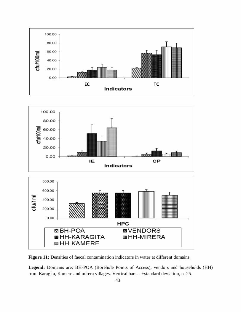
43
Figure 11: Densities of faecal contamination indicators in water at different domains.
Legend: Domains are; BH-POA (Borehole Points of Access), vendors and households (HH)
from Karagita, Kamere and mirera villages. Vertical bars = +standard deviation, n=25.
TC EC
44
Table 10: Spatial variation on microbiological quality of water at different domains
Domains EC TC IE CP HPC
BH-POA 2.23a 22.41a 0.09a 0.02a 320.70a
VENDORS 12.73ab 57.00b 9.53ac 5.66ab 552.00b
HH-KARAGITA 17.92b 53.40b 51.60b 12.80b 553.00b
HH-MIRERA 24.12b 71.60b 34.6bc 5.48ab 583.20b
HH-KAMERE 17.76b 69.48b 64.36b 9.16b 510.4b
Legend: Domains are; borehole points of access (BH-POA), Vendors and Households (HH) in
Karagita, Mirera and Kamere villages. Means in a column followed by different letters are
significantly different at p<0.05 by LSD.
4.4 Relationship between faecal contamination indicators and physicochemical parameters
Relationships between parameters measured in different water sources are shown in Tables 11,
12 and 13. From these results, minor significant relationships occurred between parameters in all
borehole waters (direct and point of access). Physico-chemical parameters did not show any
great influence on microbial parameters. However, it is notable that HPC from direct borehole
waters had positive and significant correlation with temperature (Table 11). There were
significant correlations between E. coli (EC) and all the microbiological faecal contamination
indicators in surface water (Table 13).
Table 11: Correlation between microbiological and physicochemical parameters in borehole direct
sources
EC TC IE CP HPC TEMP DO pH
EC _ _ _ _ _ _ _ _
TC 0.300 _ _ _ _ _ _ _
IE 0.223 0.090 _ _ _ _ _ _
CP -0.64 0.080 -0.044 _ _ _ _ _
HPC 0.059 -0.139 -0.064 0.152 _ _ _ _
TEMP 0.047 -0.006 0.176 -0.032 0.258** _ _ _
DO 0.042 -0.014 0.002 0.080 0.062 0.138 _ _
Ph -0.014 0.163 0.008 -0.173 -0.248** -0.365** -0.144 _
E. COND -0.120 0.076 0.150 -0.184 -0.320** -0.101 0.083 0.478
**Correlation is significant at P<0.05, (2 tailed, N=64)
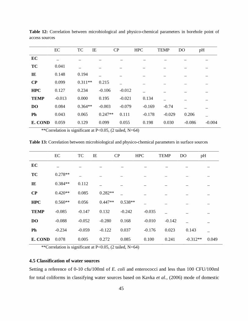
45
Table 12: Correlation between microbiological and physico-chemical parameters in borehole point of
access sources
EC TC IE CP HPC TEMP DO pH
EC _ _ _ _ _ _ _ _
TC 0.041 _ _ _ _ _ _ _
IE 0.148 0.194 _ _ _ _ _ _
CP 0.099 0.311** 0.215 _ _ _ _ _
HPC 0.127 0.234 -0.106 -0.012 _ _ _ _
TEMP -0.013 0.000 0.195 -0.021 0.134 _ _ _
DO 0.084 0.364** -0.003 -0.079 -0.169 -0.74 _ _
Ph 0.043 0.065 0.247** 0.111 -0.178 -0.029 0.206 _
E. COND 0.059 0.129 0.099 0.055 0.198 0.030 -0.086 -0.004
**Correlation is significant at P<0.05, (2 tailed, N=64)
Table 13: Correlation between microbiological and physico-chemical parameters in surface sources
EC TC IE CP HPC TEMP DO pH
EC _ _ _ _ _ _ _ _
TC 0.278** _ _ _ _ _ _ _
IE 0.384** 0.112 _ _ _ _ _ _
CP 0.420** 0.085 0.282** _ _ _ _ _
HPC 0.560** 0.056 0.447** 0.538** _ _ _ _
TEMP -0.085 -0.147 0.132 -0.242 -0.035 _ _ _
DO -0.088 -0.052 -0.280 0.168 -0.010 -0.142 _ _
Ph -0.234 -0.059 -0.122 0.037 -0.176 0.023 0.143 _
E. COND 0.078 0.005 0.272 0.085 0.100 0.241 -0.312** 0.049
**Correlation is significant at P<0.05, (2 tailed, N=64)
4.5 Classification of water sources
Setting a reference of 0-10 cfu/100ml of E. coli and enterococci and less than 100 CFU/100ml
for total coliforms in classifying water sources based on Kavka et al., (2006) mode of domestic
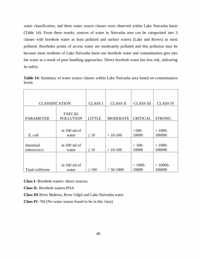
46
water classification, and three water source classes were observed within Lake Naivasha basin
(Table 14). From these results, sources of water in Naivasha area can be categorised into 3
classes with borehole water as least polluted and surface waters (Lake and Rivers) as most
polluted. Boreholes points of access water are moderately polluted and this pollution may be
because most residents of Lake Naivasha basin use borehole water and contamination gets into
the water as a result of poor handling approaches. Direct borehole water has less risk, indicating
its safety.
Table 14: Summary of water source classes within Lake Naivasha area based on contamination
levels
CLASSIFICATION CLASS I CLASS II CLASS III CLASS IV
PARAMETER
FAECAL
POLLUTION LITTLE MODERATE CRITICAL STRONG
E. coli
in 100 ml of
water ≤ 10 > 10-100
>100-
10000
> 1000-
100000
Intestinal
enterococci
in 100 ml of
water ≤ 10 > 10-100
> 100-
10000
> 1000-
100000
Total coliforms
in 100 ml of
water ≤ 100 > 50-1000
> 1000-
10000
> 10000-
100000
Class I- Borehole waters- direct sources.
Class II- Borehole waters-POA
Class III River Malewa, River Gilgil and Lake Naivasha water
Class IV- Nil (No water sourse found to be in this class)
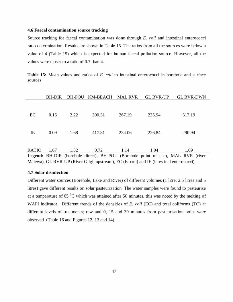
47
4.6 Faecal contamination source tracking
Source tracking for faecal contamination was done through E. coli and intestinal enterococci
ratio determination. Results are shown in Table 15. The ratios from all the sources were below a
value of 4 (Table 15) which is expected for human faecal pollution source. However, all the
values were closer to a ratio of 0.7 than 4.
Table 15: Mean values and ratios of E. coli to intestinal enterococci in borehole and surface
sources
BH-DIR BH-POU KM-BEACH MAL RVR GL RVR-UP GL RVR-DWN
EC 0.16 2.22 300.31 267.19 235.94 317.19
IE 0.09 1.68 417.81 234.06 226.84 290.94
RATIO 1.67 1.32 0.72 1.14 1.04 1.09
Legend: BH-DIR (borehole direct), BH-POU (Borehole point of use), MAL RVR (river
Malewa), GL RVR-UP (River Gilgil upstream), EC (E. coli) and IE (intestinal enterococci).
4.7 Solar disinfection
Different water sources (Borehole, Lake and River) of different volumes (1 litre, 2.5 litres and 5
litres) gave different results on solar pasteurization. The water samples were found to pasteurize
at a temperature of 65 0C which was attained after 50 minutes, this was noted by the melting of
WAPI indicator. Different trends of the densities of E. coli (EC) and total coliforms (TC) at
different levels of treatments; raw and 0, 15 and 30 minutes from pasteurisation point were
observed (Table 16 and Figures 12, 13 and 14).
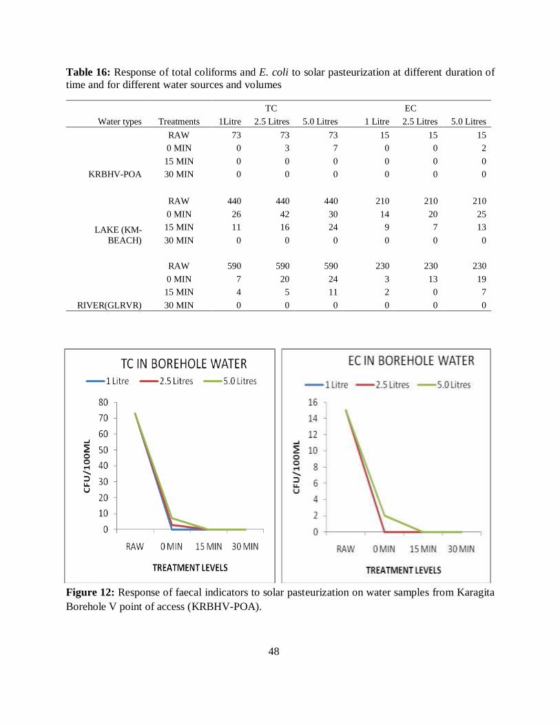
48
Table 16: Response of total coliforms and E. coli to solar pasteurization at different duration of
time and for different water sources and volumes
Water types Treatments
TC EC
1Litre 2.5 Litres 5.0 Litres 1 Litre 2.5 Litres 5.0 Litres
KRBHV-POA
RAW 73 73 73 15 15 15
0 MIN 0 3 7 0 0 2
15 MIN 0 0 0 0 0 0
30 MIN 0 0 0 0 0 0
LAKE (KM-
BEACH)
RAW 440 440 440 210 210 210
0 MIN 26 42 30 14 20 25
15 MIN 11 16 24 9 7 13
30 MIN 0 0 0 0 0 0
RIVER(GLRVR)
RAW 590 590 590 230 230 230
0 MIN 7 20 24 3 13 19
15 MIN 4 5 11 2 0 7
30 MIN 0 0 0 0 0 0
Figure 12: Response of faecal indicators to solar pasteurization on water samples from Karagita
Borehole V point of access (KRBHV-POA).
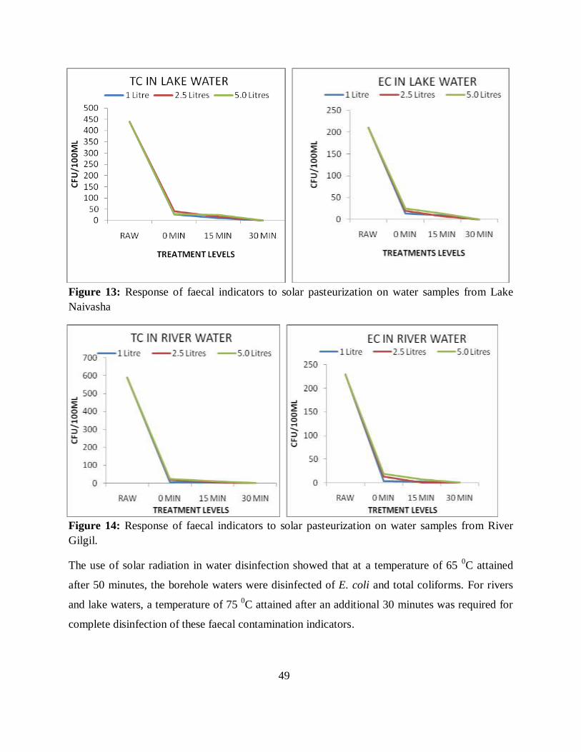
49
Figure 13: Response of faecal indicators to solar pasteurization on water samples from Lake
Naivasha
Figure 14: Response of faecal indicators to solar pasteurization on water samples from River
Gilgil.
The use of solar radiation in water disinfection showed that at a temperature of 65 0C attained
after 50 minutes, the borehole waters were disinfected of E. coli and total coliforms. For rivers
and lake waters, a temperature of 75 0C attained after an additional 30 minutes was required for
complete disinfection of these faecal contamination indicators.
50
CHAPTER FIVE
DISCUSSION
5.1 Physicochemical parameters
The results of this study show that all the physicochemical parameters from all the water sources
in Lake Naivasha basin were within the recommended standards of WHO, US-EPA and NEMA
(appendices 1 and 2) for drinking water. These results are also similar to those obtained in water
sources from Aboekuta, Nigeria (Shittu et al., 2008). Higher levels of electrical conductivity
were recorded from borehole water than surface water sources as expected. This is attributed to
high levels of dissolved minerals found in ground water and in particular fluoride which has been
recorded in borehole waters within the region (Matofari, 2006). High values of dissolved oxygen
in rivers and borehole waters at the points of access (POA) was due to aeration caused by the
flow of water in the rivers and high pressures as the water flows from over-head reservoirs to the
lower distribution taps connected with hose pipes (Plate 3a) where sampling was conducted. The
values of dissolved oxygen and electrical conductivity varied significantly with respect to
sampling sites for all the water sources categories; Borehole Direct sources, Borehole Point of
Access (BH-DIR, BH-POA) and Surface sources. This may be attributed to variation in pollution
levels, mineral content as well as the volume of the water mass in relation to pollution sources.
For Borehole Points of Acess (BH-POA) sources, temperature did not show significant variation
with respect to sampling sites, this could have been due to heating from the sun which tend to
warm the water in the reservoir in a more uniformly manner within the entire Lake Naivasha
basin. Lower values of dissolved oxygen in samples from vendors and household could have
been contributed by the source from which the water was collected. Such samples with low
dissolved oxygen may have been collected from the Lake where high organic pollution occurs as
evidenced by high levels of Heterotrophic Plate Count (HPC). In addition, further fall in
dissolved oxygen levels could have resulted from storage time within the vendors and household
domain. Water sampled from vendors were sometimes giving electrical conductivity values
lower than expected values from borehole waters, this was an additional evidence that some of
the water being sold to the consumers by the vendors could have been collected from the surface
sources or was a mixture of borehole and surface sources. Physicochemical parameters obtained
51
in samples from vendors and households from the three villages did not vary significantly,
showing that majority of the water sampled here could have had a common source which was
traced to be Borehole Point of Access (BH-POA) sources.
5.2 Microbiological Parameters
Groundwater has generally been observed to be of good microbial quality and boreholes are
considered to be the cleanest water sources for domestic use. Globally, over 80% of the
population relies on ground water for domestic supplies (Cronin et al., 2008). This is because
deep aquifers are protected from pathogenic contamination which are effectively removed by soil
particles, die offs and predation (Dufour et al., 2003). In the current study, the presence of faecal
indicators; E. coli, total coliforms, intestinal enterococci, and C. perfringens can be attributed to
poor handling of water at points of access. As compared to borehole-Poit of Access samples,
water samples from boreholes-Direct sources had very low absolute values of the
microbiological densities with majority of these parameter values being zero per 100 ml. Direct
bore source at Denmark Company in Kenya (DCK) gave poor microbial quality as compared to
other direct sources. This could be due to influence from the lake water since the site is in close
proximity to the lake than other direct borehole sites. On a general perspective, the quality of
water from Borehole-Direct water sources in Lake Naivasha basin was within the recommended
standards by WHO, US Environmental Protection Agency and Nationa Environmental protection
Agency Kenya (NEMA-Kenya). This is because 88% of the samples analysed were free of faecal
contamination and there were no positive results for the presence of faecal contamination noted
in any two consecutive sampling occasions. This result showed that Borehole-Direct sources are
generally fit for human consumption but due to a few incidences of positive results for faecal
contamination, disinfection of these water sources is necessary before consumption for surety of
the health safety to the consumer.
In general, Borehole-Point of Access gave higher mean values than the Borehole-Direct sources
indicating increased exposure of water to contamination through handling at the water supply
points and reservoirs. At the points of use, water samples were obtained without sterilizing the
pipes. The reason was to give the actual status in terms of microbial quality of the water being
availed to the community from these sources. This is similar to an approach applied by Wright in
52
2004 in Zambia (Wright et al 2004). Sterilization may often result to under estimation of the
contamination status especially in supply points where poorly handled hose-pipes are connected
to the taps as was the case at the borehole water supply points in Naivasha. In addition, use of
hose pipes which are held with dirty hands, dragged on the dumpy grounds and on the back of
the donkeys as the supply process contribute further to water contamination at the points of use.
This condition is made worse by the dung from the donkeys which were commonly present on
the same dumpy grounds within the water selling points. In this regard, sampling of the water
without sterilization allowed the capturing of the contribution of all these contamination
practices onto the quality of water supplied to the community. With this in mind, most reliable
and preventive measure to contamination of water sources could be through protection of all the
sources (Figueras and Borrego, 2010). Karagita borehole II at the point of access (KRBHII-
POA) and Karagita borehole V at the point of access (KRBHV-POA) gave higher mean values
than Karagita borehole I at the point of access (KRBHI-POA) and Karagita borehole III at the
point of access (KRBHIII-POA). This together with the significance spatial variation in the mean
values of microbial parameters from borehole points of access (BH-POA) could have been
caused by the variation in sanitation levels by different borehole owners. This result is in
agreement with the study on bacteriological quality of borehole water used by students at the
University for Development Studies, Navrongo Campus in Upper-East Region of Ghana,
(Adetunde et al., 2010). However, the water quality at the Borehole-Poin of Acess was not
within the recommended standards by WHO, US Environmental Protection Agency and NEMA-
Kenya. Due to this, disinfection of water from these sources should be a mandatory procedure
before its consumption. This is because water of such status are of public health significance
considering the possibility of the presence of other bacteria, protozoa and enteric viruses that are
implicated in gastro-intestinal waterborne diseases and the low infectious dose for these
waterborne pathogens, (Shittu et al., 2008).
During this study, seasonality in the density of faecal contamination indicators was not
evidenced in both the Borehole-Direct and Borehole-Point of Access sources. These sources
showed no significant variation with respect to time of sampling (April, May, June and July).
This was an indication that there was no weather variable that had significant influence on the
density of faecal contamination indicators for the entire study period. An additional reason to
53
support this could have been that, the population of the local community which use/access the
borehole throughout the study period remained the same. This consistence in numbers of people
who accessed the borehole could have been due to the reason that the intensity of rainfall during
that same period was not enough to prevent a significant portion of the population within the
Lake Naivasha Basin from visiting Borehole-Point of access sources to collect water. Therefore,
on any day when it rained, a few people switched to using rain harvested water and hence the
degree of contamination at the Borehole-Point of access did not change greatly with respect to
sampling times.
The poor quality of surface water sources (River Malewa and River Gilgil upstream and
downstream as well as Lake Water at Kamere beach) could have been contributed by
anthropogenic activities in the catchment within the streams and at the beach. These pollution
practices noted entailed; in-stream and lake-shore activities such as; laundry, cars and donkeys
driven into the river/lake to fetch water by vendors as well as large herds of cattle and wild
animals which defecate and urinate in the water when they access these system to drink or even
to graze on the riparian vegetation. Similar pollution practices have been reported in other Rift
valley Rivers (Mokaya et al., 2004; Yillia et al., 2009). These studies also noted that cows were
dominant contributors to faecal contamination in most rivers, raising concern over the health of
human and other animals. Therefore, there is need to adopt measures to improve the quality of
surface water sources as they were far much above the recommended standards by various
drinking water quality monitoring agencies.
Within River Gilgil, down-stream water sampling point was found to have higher
microbiological density values than up-stream water sampling points. This indicated an increase
in faecal pollution loading as the river flows across the animal grazing field, residential places as
well as flower farms. This result is in agreement with that of Shawky et al., (2007) who showed
that there was gradual increase in the bacterial counts from up-stream to down-stream from El-
Qanater to Damietta of river Nile. They attributed this observation to domestic, sewage and
agricultural effluents discharge. In addition, a study on the quality of River Nile Water at Cairo
Region in Egypt also attributed its poor water quality to anthropogenic influences (Hala, 2007).
The higher mean density of microbiological parameters reported in samples from River Gilgil
54
than River Malewa despite both rivers draining through flower farms and residential areas could
be due to difference in water mass. River Malewa is bigger than River Gilgil and this could have
resulted in dilution effects which lowered the microbial density levels. The water quality of the
surface sources was not within the recommended standards by WHO, US Environmental
Protection Agency and NEMA-Kenya as it was observed that 100% of the samples were positive
for faecal contamination. The result on surface water sources is the same as the finding on
assessment of the microbial quality of river water sources in rural Venda communities in South
Africa, (Obi et al., 2002). As a remedial measure, there is need to disinfect water from these
sources before its consumption by human beings to eliminate disease causing organisms (Shittu
et al., 2008). The significant variation in mean density of faecal contamination indicators with
respect to time of sampling (April, May, June and July) was an indication that unlike the
borehole sources, surface sources based on their microbiological quality were more susceptible
to influence of weather variables e.g. rainfall. The few incidences of rain that occurred during the
duration of this study were noted to have an influence on the microbiological quality of surface
water which is in agreement with results of a similar study in United States by Hatfield and
Prueger, (2004).
Household water security comprise of water availability, good quality, easier accessibility and
availability for consumption at household level (Asare, 2004). Water at the household and
vendors domain was noted to be of poorer quality as compared to the Borehole-Point of Access
sources. This was generally due to poor water handling practices at both the house hold and
vendors domain. Insignificant difference in the means of microbial parameters between
Borehole Point of Access, vendors and household from the three villages (Karagita, Mirera and
Kamere) indicated that majority of the households and vendors had their water contaminated
through poor handling in a more or less the same degree. The positive and significant correlation
between Heterotrophic Plate Count and temperature in borehole direct sources indicates that
temperature could be one of the factors influencing microbial growth in borehole water. The fact
that there was no significant correlation between temperatures with faecal indicator micro-
organisms means that faecal contamination in direct borehole water was of minor consequence in
causing public health concerns. The significant correlations between E. coli and all microbial
faecal indicators of pollution apart from total coliforms in surface water sources could probably
55
be an indicator that contamination with organic matter is of faecal origin. Lack of significant
correlations between E. coli and total coliforms in surface water could indicate that total
coliforms could have proliferated in the environment and there was no direct relationship with E.
coli of recent origin. This low correlation between microbiological indicator organisms has also
been a major issue for discussion in a study within the wooded watersheds of the Southern
Piedmont (Dwight and Dinku, 1999).
The ratios of E. coli to intestinal enterococci of different water sources were closer to 0.7 than
4.0. This showed that the major source of pollution into the water sources within Lake Naivasha
basin were most probably of non-human warm blooded animals’ origin. Indeed, domestic and
wild animals were a common occurrence at the precincts of water sources. Vendors were also
using donkeys for transportation of water to the consumers. In addition, domestic and wild
animals were also noted to be visiting the lake and rivers for drinking purposes. This result was
the same as what was reported for a river in North Area of Wigry National Park where it was
found that source of faecal contamination was majorly coming from flows arising from other
arable-forestry-pasture-meadow catchments as expressed by a larger number of streptococci than
E. coli, (Niewolak, 1999).
5.3 Solar radiation disinfection
Solar disinfection was able to eliminate E. coli and total coliforms from all the water sources
(rivers, lake and borehole) and hence proved to be a small scale cost-effective method of
disinfecting water for domestic consumption and reducing incidences of waterborne diseases.
The duration of time needed for complete eradication of E. coli and total coliforms through solar
pasteurization was probably due to the density of these microbes in the water/class of the water.
More time of exposure to radiation for disinfection was required for highly polluted water than
for less polluted ones. Similar studies in Kavaraipettai, Tamil Nadu, and India on water quality
improvement also confirmed that there was a reduction of coliforms in the waste water after
subjecting it to solar disinfection (Negar and Metcalf, 1999). In these areas, like in many parts of
Africa, maximum temperature occurs around 1 p.m. and this therefore increases the efficiency of
the solar pasteurization kit in disinfection of water. The solar disinfection kit used for domestic
water purification in Lake Naivasha basin eliminated 99.99% of coliforms after an additional 30
56
minutes from pasteurization point. This innovative solar disinfection system has additional
advantages; the kit being portable, it is cost-effective and it can be fabricated in Africa for US$ 8
(approximately Kenya Shillings 640). The unit incorporates the principle of reflection to increase
solar intensity and large units can also be manufactured for large scale use. Since all the
materials are available locally, the unit can be manufactured locally by the local people. The
most valid and reinforcing reason to the use of this kit is the fact that day temperatures above 25
0C occur at the tropics for more than 10 months in a year and as such this innovative solar
disinfection unit can be of much benefit in Lake Naivasha Basin.
This solar pasteurization technology can be a better approach in water quality improvement.
Indeed, microbial contamination of drinking water is associated with incidences of
gastrointestinal illnesses in many studies. In addition, 88% of such reported cases occur as a
result of contaminated water, poor hygiene, and poor sanitation (WHO, 2002). The technology
can be of paramount benefit to human health in Naivasha Lake basin where rampant cases of
diarrhea have been reported. Based on this, WHO guideline which restricts water services
providers to have water safety plans to ensure consistent supply of safe drinking water is of great
importance as far as the quality of water is concerned. The approach manages the risks
associated with consumption of contaminated drinking water from the catchment level to the
treatment plant and then to the household level at consumers’ taps (Figueras and Borrego, 2010).
It aims at ensuring catchment conservation and protection, protection of water at the sources,
during and after treatment through proper storage and distribution and awareness creation to the
distributors and consumers about their responsibilities in maintenance of the good water quality.
This would be a major achievement to Naivasha Water and Sanitation Company (NAWASCO)
especially in line with their goals of upgrading water and sanitation services within Naivasha
region. Due to variety of risk factors, in the spread, transmission and acquisition of waterborne
and water related illnesses, interventions for their prevention not only enhance water availability
but also tries to improve the proper disposal of human faeces, improve water quality and quantity
as well as personal and environmental hygiene.
Microbiological assessment of drinking water at source and point of use has also become a major
issue due to realization of the impact of poor water quality with microbiological contamination at
57
household level on public health. This health risk is caused by various factors among which
water quality plays a significant role. Assessment of drinking water quality at public and private
domains aims at ensuring that consumers use water that is free from disease causing organisms
and protects them from water related diseases (Jensen et al., 2002). The contamination may arise
from transportation of bacteria laden water that is rich in organic matter and suspended particles
through overland flow into surface water, while in ground water it is through sub-surface flow
into aquifers, especially when the aquifer is shallow and unconfined. Due to open access to
surface water ecosystems, bacteria density are often high in rivers ranging between 4-5 log units
compared to ground waters with zero E. coli densities in deep wells and up to 3 log units in
polluted shallow wells (Cronin et al., 2008). This is of particular interest in many developing
countries where a large number of the population still depends on surface water sources use as
their source of domestic water.
Based on reference adapted from Kavka et al., (2006), the water in Lake Naivasha basin can be
categorized into classes I and II for Borehole-Direct and Borehole-Point of Access sources
respectively. Surface sources on the other hand fall under class III. This classification was in
agreement with the classification made on the study on bacteriological monitoring of River
Water Quality in the North Area of Wigry National Park. In that study, the density of the
examined indicator bacteria found put the river into (class III of purity), (Niewolak 1999).

58
CHAPTER SIX
CONCLUSION AND RECOMMENDATION
6.1 Conclusion
Based on the findings of this study, the following conclusions can be drawn;
I. Water from all Borehole direct sources within Lake Naivasha basin is of good bacterial
quality and the good quality does not change over time. Water from all the borehole point
of access sources within the basin are of poor quality and this poor quality does change
over time. Water from surface sources within the basin is also of poor quality, these
sources are exposed to numerous contaminants hence their poor microbial quality levels
undergo variation over time.
II. Poor human water handling practices within Lake Naivasha basin result to degradation of
the bacterial quality of domestic water.
III. The E. coli to intestinal enterococci ratios were noted to be closer to 0.7 than to 4.0 this
indicates that the major contributor of faecal contamination into various water sources
with Lake Naivasha basin is non-human warm blooded animals.
IV. Solar pasteurization kit has the potential of disinfecting domestic water based on the
prevailing solar radiation conditions within Lake Naivasha basin.
6.2 Recommendations
Several recommendations can be drawn from the result of this study. They are necessary in
improving the quality of water available for human consumption and reducing the incidences of
waterborne disease outbreaks. They are;
I. Awareness creation on personal and environmental hygiene including maintenance of
high sanitation standards in water distribution points as well as in water storage and
distribution containers.
II. Need to put in place proper sewage disposal and treatment measures to reduce the amount
of raw sewage that finds its way into the water sources.
59
III. Need to supply the communities with clean piped water at their households to keep the
population away from the surface sources (rivers and lake). This can assist in protecting
these water sources from further quality degradation and pollution.
IV. An urgent need to focus on the means and ways of controlling pollution of these
community water sources by other organic and inorganic materials through proper solid
and liquid waste disposal and regular water monitoring programmes to be established for
all water sources in Lake Naivasha basin.
V. Recommending the use of other faecal contamination source tracking approaches like
molecular techniques to increase the reliability and accuracy in tracking the sources of
faecal contamination in controlling faecal pollution.
VI. Availing and emphasizing the use of affordable, cheap and locally available and
environmentally friendly point of use/household water treatment approaches. These
include solar radiation disinfection using water pasteurization kits. This is required in
rural and informal urban settlement (slams) as it is the case in Lake Naivasha basin where
water is obtained from public standpoints, rivers, lake or from resellers (vendors).

60
REFERENCES
Acher A., Fischer R., Turnheim B. and Manor Y. (1997). Ecologically friendly wastewater
disinfection techniques. Water Resource. 31:1398-1404.
Adetunde L.A. and Glover R.L.K. ( 2010). Bacteriological Quality of Borehole Water Used by
students’ of University for Development Studies, Navrongo Campus in Upper-East Region of
Ghana. Current Research Journal of Biological Science. 2(6): 361-364.
American Public Health Association (APHA) (2005). Compendium of Methods for the
Microbiological Examination of Foods, 19th Edition. Washington, DC.
Araujo M. (2001). Evaluation of fluorogenic TSC agar for recovering Clostridium perfringens in
groundwater samples. Water Science and Technology. 43:201–204.
Asare K.O. (2004). Hydrogen Reduction of Metal Ions: An Electrochemical Model,
Hydrometall. Proceedings in the International Symposium. 2: 1151–1165.
Ashbolt N. J., Grabow W.O.K. and Snozzi M. (2001). Indicators of microbial water quality. In:
Fewtrell L, Bartram J, eds. Water quality: Guidelines, standards and health Assessment of risk
and risk management for water-related infectious disease. World Health Organization Water
Series. London, IWA Publishing. 289–315.
Bakare A.A., Lateef A., Amuda O.S. and Afolabi R.O. (2003). The Aquatic toxicity and
characterization of chemical and microbiological constituents of water samples from Oba
River, Odo-oba, Nigeria. Asian Journal of Microbiology, Biotechnology and Environmental
Sciences. 5: 11–17.
Beveridge M.T. (1988). Genetic studies of laboratory reared Mytilus odilis. Genotype specific
selection in relation to salinity. Heredity. 61: 389-400.
Bonde G.J. (1997). Bacteriological indicator of water pollution. Advance Aquatic Microbiology.
1: 273-364.
Cronin A.A., Shrestha D., Cornier N., Abdalla F., Ezard N. and Aramburu C. (2008). A review
of water and sanitation provision in refugee camps in association with selected health and
nutrition indicators – the need for integrated service provision. A journal of Water and Health.
6: 1-25.
61
Deere D., Vesey G., Ashbolt N. and Gauci M. (2002). Flow cytometry and cell sorting for
monitoring microbial cells. In: Encyclopaedia of Environmental Microbiology. Bitton, G.
(Ed.). John Wiley and Sons, New York (in press).
Doyle M.P. and Erickson M.C. (2006). “Closing the door on the fecal coliform assay: The faecal
coliform assay, the results of which have led to numerous misinterpretations over the years,
may have outlived its usefulness”. Microbe. 1: 162-163.
Dufour C., Corcione A., Svahn J., Haupt R., Poggi V., Béka’ssy A., Scimè A. and Pistoia V.
(2003). TNF-alpha and IFN-gamma are overexpressed in the bone marrow of Fanconi anemia
patients and TNF-alpha suppresses erythropoiesis in vitro. 102:2053–2059.
Dwight S.F. and Dinku M.E. (1999). Total coliform, E. coli and enterococci bacteria in grazed
and wooded watersheds of the Southern Piedmont. Proceedings of the 1999 Georgia Water
Resources Conference, held March 30-31, 1999 at the University of Georgia.
Fenlon, D.R. (1983). A comparison of Salmonella serotypes found in the faeces of gulls feeding
at sewage works with serotypes in sewage. Journal of Hygiene. 41: 47-52.
Figueras M.J. and Borrego J.J. (2010). New perspective in monitoring drinking water microbial
quality. International Journal of Environmental Research on Public Health. 7: pp 4179-4202.
Frahm E., John V. and Obst U. (2003). Application of the fluorogenic probe technique (TaqMan
PCR) to the detection of Enterococcus spp. and Escherichia coli in water samples. Journal of
Microbiological Methods. 52: 123-131.
Framework for Action exercise of the Global Water Partnership (FFA of GWP) (2000). pp58.
George H. (2001). Use of rapid enzymatic assays to study the distribution of faecal coliforms in
the Seine River (France). Water Science and Technology, 43: 77-80.
Goverment of Kenya (2009): National Population Census. Nairobi, Government Printer.
Grabow W.O.K. (1996). Waterborne diseases: Update on water quality assessment and control.
Water South Africa. 22: 193–202.
Hala M.R. (2007). Bacterial Quality of River Nile Water at Cairo Region in Egypt. Suoseura
Helsinki — Finnish Peatland Society. 59: 1–21.
Harper D.M. and Mavuti K.M. (2004). Lake Naivasha, Kenya: Ecohydrology to guide the
Management of a tropical protected area. Ecohydrology & Hydrobiology. 4: 287-305.
62
Hatfield J.L. and Prueger J.H. (2004). Impacts of changing precipitation patterns on water
quality. Journal of Soil and Water Conservation 59(1): 51-58.
Hoxie N.J. Davis, J.P. Vergeront, J.M. Nashold, P.D. and Blair K.A. (1997). Cryptosporidiosis-
associated mortality following a massive waterborne outbreak in Milwaukee, Wisconsin.
American Journal of Public Health. 87: 2032-2035.
http:www.solarcooker.org. Accessed on 5th November 2011.
Huss H. Reilly A. and Embarek P. (2000). Prevention and control of hazards in seafood. Food
Control. 11: 149-156.
Jay J.M. (1992). Modern Food Microbiology. Microbiological Indicators of food safety and
quality, Principles and Quality control, and microbiological criteria. New York: Van Nostrand
Reinhold.
Jensen P.K., Jeroen H.J.E., Jayasinghe G., Hoek W., Cairncross S. and Dalsgaard A. (2002).
Domestic transmission routs of pathogens. The problems if in-house contamination of
drinking water during storage in developing countries. Tropical Medicine and International
Health. 7(7): 604-609.
Japan International Cooperation Agency (JICA) (2003). Preparatory study report on the water &
sewarage System of Naivasha Town in Kenya.
Karr J.R. (1999). Defining and measuring river health. Freshwater biology. 41: 221-234.
Kavka G.G., Kasimir G.D. and Farnleitner A.H. (2006). Microbiological water quality of the
river Danube (km 2485 - km 15). Longitudinal variation of pollution as determined by
standard parameters. Arch Hydrobialogy Suppliment 113 Large Rivers. 10: 79-86.
Kirby R.M., Bartram B. and Carr R. (2003). Water in food production and processing-Quality
and quality concerns. Food Control. 14: 283-299.
Kjellen M. and Mc Granaham G. (2006). Informal water vendors and the urban poor.
International Institute for Environment and Development (IIED). http://www.IIied.org
/HS/publications.
Kondro W. (2000). E. coli outbreak deaths spark judicial inquiry in Canada. The Lancet. 355:
2058-2070.
63
Kramer M.H. Herwaldt B.L. Calderon R.L. and Jurannek, D.D. (1996). Surveillance for
waterborne-disease outbreaks-United States, 1993-1994. CDC surveillance Summaries
MMWR Week Report. 45: 1-33.
LakeNet (2003). Naivasha. Accessed 23-July, 2003, from the World Wide Web:
http://www.worldlakes.org/initiative/naivasha_profile.htm
Lawand T.A., Ayoub J. and Gichenje H. (1997). Solar disinfection of water using transparent
plastic bags. RERIC International Energy Journal. 19: 1-7.
M’CLeen P. (2001). Spartial analysis of water quality and eutrophication controls of lake
Naivasha, Kenya. Applied and Environmental Microbiology 51: 10-112
Maddock I. (1999). The importance of physical habitat assessment for evaluating river health.
Freshwater biology 41: 373-391.
Mageau, M.T., Costanza, R. and Ulanowicz R.E. (1995). The development and initial testing of a
quantitative assessment of ecosystem health. Ecosystem Health 1 (4), 201–213.
Matofari, W.J. (2006). How safe is water we drink? Determination of chemical and
bacteriological water sources in Njoro, Nakuru district, Kenya. Egerton University Journal of
Science and Technology. Vol. (6).
Meinhardt P.L. (2009). Waterborne Disease and Water Pollution: The Public Health Impact in
Rural Communities 8th Annual Conference on Rural Health Geneva, New York – September
22, 2009
Metcalf B. and Logvin M. (1999). Solar now; an energy primer and guide to low cost solar
cooking, solar tea, solar hot water. Solar Now Publications, Sacramento, Calif. 1: 26-27.
Meyer J.L. (1997). Stream health: incorporating human dimension to advance stream ecology.
Journal of North American Benthological Society. 16: 437-447.
Mireri C. (2005). Challenges Facing the Conservation of Lake Naivasha, Kenya. FWU, Vol. 3,
Topics of Integrated Watershed Management – Proceedings
Mokaya S.K., Mathooko J.M. and Leichtfried M. (2004). Influence of anthropogenic activities of
water quality of a tropical stream ecosystem. African Journal of Ecology. 42: (4), 281-288.
Mossel D.A.A., Corry J.E.L., Struijk C.B., and Baird R.M. (1995). Essentials of the
Microbiology of Foods: A Textbook of Advanced Studies. London, John Wiley & Sons, 1995.
New York, pp. 489-522.
64
Negar S. and Metcalf R.H. (1999). Enhancement of Solar Water Pasteurisation with Reflectors.
Applied and Environmental Microbiology. 65 (2): 859-861.
Niewolak S. (1999). Bacteriological Monitoring of River Water Quality in the North Area of
Wigry National Park. Polish Journal of Environmental Studies. 9 (4): 291-299
Njeminski E.C., Bellamy W.D. and Moss L.R. (2000). Using surrogates to improve plant
performance. Journal of the American Water Works Association. 92: 67–78.
Noble R.T., Moore D.F., Leecaster M.K., McGee C.D. and Weisberg S.B. (2003). Comparison
of total coliform, feacal coliform, and enterococcus bacterial indicator response for ocean
recreational water quality testing. Water Research. 37: 1637-1643.
Obi C.L., Potgieter N., Bessong P.O. and Matsaung G. (2002). Assessment of the microbial
quality of river water sources in rural Venda communities in South Africa. Water South
Africa. 28 (3).
Olsen A.R. and Hammack T.S. (2000). Isolation of Salmonella spp.from the housefly, Musca
domestica L., and the damp fly, Hydrotea aenescens, at caged layer houses. Journal of Food
Protection. 63: 958-960.
Otiang'a E.O. and Oswe I.A. (2007). Human impact on lake ecosystems: the case of Lake
Naivasha, Kenya. African Journal of Aquatic Science. 32 (1): 79-88.
Oomen L.C., TenHave-Opbroek A.A., Hageman P.C., Oudshoorn-Snoek M., Egberts J., Van der
Valk M.A., Calafat J. and Demant P. (1990). Foetal mouse alveolar type II cells in culture
express several type II cell characteristics found in vivo, together with major
histocompatibility antigens. American Journal of Respiratory Cell and Molecular Biology 3:
325-39.
Parish M.E. (1998). Coliforms, Escherichia coli and Salmonella serovars associated with a
citrus-processing facility implicated in a salmonelosis outbreak. Journal of Food Protection.
61: 280-284.
Poté J., Goldscheider N., Haller L., Zopfi J., Khajehnouri F. and Wildi W. (2009). Origin and
spatial–temporal distribution of faecal bacteria in a bay of Lake Geneva, Switzerland.
Environmental Monitoring and Assessment. 154: 337-348.
Robert C. (2005). The microbiology of solar water pasteurization, with applications in East
Africa, California State University, Sacramento Press.
65
Rompré A., Servais P., Baudart J., De-Roubin R.M. and Laurent P. (2002). Detection and
Enumeration of coliforms in drinking water :current methods and emerging approaches.
Journal of Microbiological Methods. 49: 31-54.
Rufener S., Daniel M., Hans-Joachim M. and Rolf W. (2010). Quality of Drinking-water at
Source and Point-of consumption-Drinking Cup As a High Potential Recontamination Risk:
A Field Study in Bolivia. Journal of Health Population Nutrition. 1: 1-120.
Scott T.M., Rose J.B., Jenkins T.M., Farrah S.R. and Lukasik J. (2002). Microbial source
tracking: current methodology and future directions. Applied Environmental Microbiology. 68:
5796-5803.
Shawky Z.S. and Saleh A.R. (2007). Management of a tropical protected area. Egyptian Journal
of Aquatic Research. 33(1): 301-311.
Shittu O.B., Olaitan J.O. and Amusa T.S. (2008). Physico-Chemical and Bacteriological
Analyses of Water Used for Drinking and Swimming Purposes in Abeokuta, Nigeria. African
Journal of Biomedical Research. 11; 285-290
Shuval H.I., Yekutiel P., and Fattal B. (1996). Epidemiological Evidence for Helminth and
Cholera Transmission by vegetables irrigated with waste-water-Jerusalem – A case-study.
Water Science and Technology 17: 433-442.
Simpson J.M., Santo D.J.W. and Reasoner D.J. (2002). Microbial source tracking: state of the
science. Environtal Science Technology. 36: 5279-5288
Sinton L.W., Hall C.H., Lynch P.A. and Davies-Colley R.J. (2002). Sunlight inactivation of fecal
indicator bacteria and bacteriophages from waste stabilization pond effluent in fresh and
saline waters. Applied Environtal Microbiology. 68: 1122-1131.
Stewart J., Ellender R.D., Gooch J.A., Jiang S., Myoda S. and Weisberg S. (2003).
Recommendations for microbial source tracking: lessons from a methods comparisons study.
Journal of Water Health. 1: 225–231.
Sueiro R.A. (2001). Evaluation of Coli-ID and MUG Plus media for recovering Escherichia coli
and other coliform bacteria from groundwater samples. Water Science and Technology. 43:
213–216.
Thomas J.S. and Durham B. (2003). Integrated Water Resource Management: looking at the
whole picture*1. Desalination. 156: 21-28
66
Urban J.E. and Broce A. (2000). Killing of flies in electrocuting insects traps releases bacteria
and viruses. Current Microbiogy. 41: 267-270.
Vesey G., Narai J., Ashbolt N., Williams K.L. and Veal D.A. (1994) Detection of specific
microorganisms in environmental samples using flow cytometry. In: Methods in Cell Biology.
Darzynkiewicz, Z., Robinson, J. P. and Crissman, H. A. (Eds.). 42. Academic Press Inc.,
Weaver R., Entry J. and Alexandria G. (2005). Numbers of faecal streptococci and Escherichia
coli in fresh and dry cattle, horse and sheep manure. Canadian Journal of Microbiology. 51:
847-851.
Wilconsin (1993). Antibiotics to a range of Staphylococcus aureus and Escherechia coli heat
shoch protein. Antimicrobial Chemother. 27: 459-468.
World Health Organization (WHO) (2002). Health-based monitoring of recreational waters: the
feasibility of a new approach (the “Annapolis Protocol”). World Health Organization,
Geneva.
Wright J., Gundry S. and Conroy R. (2004). Household drinking water in developing countries.
A systematic review of microbiological contamination beteen source and point of use.
Tropical Medicine and international health. 9: 106-117.
Yillia P.T., Kreuzinger N., Mathooko J.K. and Ndomahina E.T. (2009). Microbial risk
assessment with the OAEL approach at water abstraction points in rural Kenya. Physics and
Chemistry of the Earth. 34: 790-798.
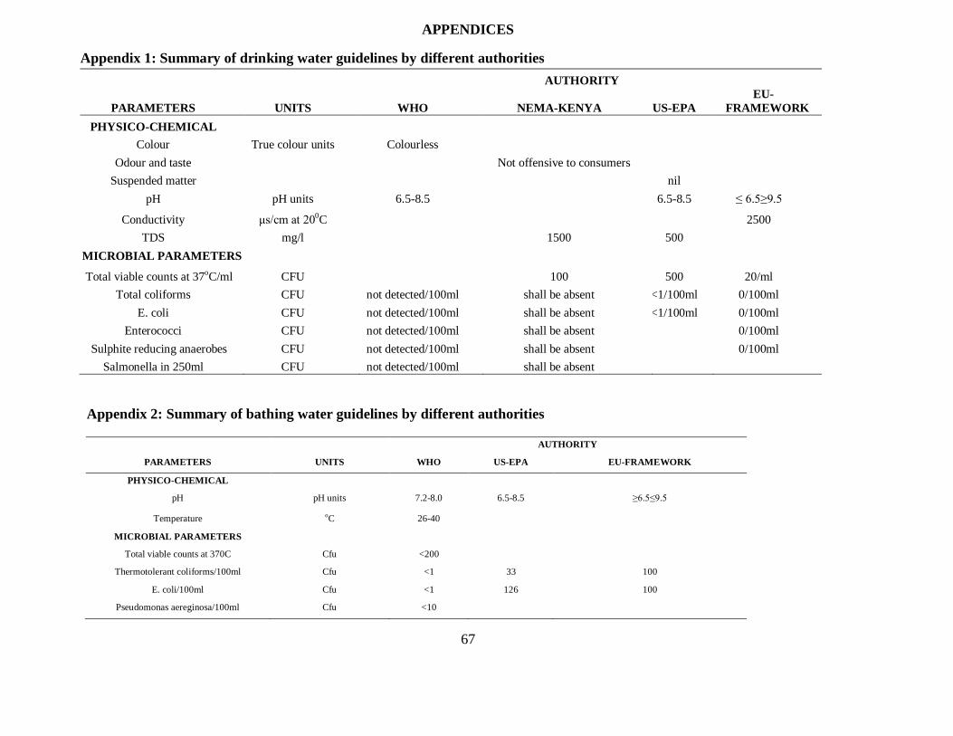
67
APPENDICES
Appendix 1: Summary of drinking water guidelines by different authorities
PARAMETERS UNITS
AUTHORITY
WHO NEMA-KENYA US-EPA
EU-
FRAMEWORK
PHYSICO-CHEMICAL
Colour True colour units Colourless
Odour and taste
Not offensive to consumers
Suspended matter
nil
pH pH units 6.5-8.5
6.5-8.5 ≤ 6.5≥9.5
Conductivity μs/cm at 200C
2500
TDS mg/l
1500 500
MICROBIAL PARAMETERS
Total viable counts at 37oC/ml CFU
100 500 20/ml
Total coliforms CFU not detected/100ml shall be absent <1/100ml 0/100ml
E. coli CFU not detected/100ml shall be absent <1/100ml 0/100ml
Enterococci CFU not detected/100ml shall be absent
0/100ml
Sulphite reducing anaerobes CFU not detected/100ml shall be absent
0/100ml
Salmonella in 250ml CFU not detected/100ml shall be absent
Appendix 2: Summary of bathing water guidelines by different authorities
PARAMETERS UNITS
AUTHORITY
WHO US-EPA EU-FRAMEWORK
PHYSICO-CHEMICAL
pH pH units 7.2-8.0 6.5-8.5 ≥6.5≤9.5
Temperature oC 26-40
MICROBIAL PARAMETERS
Total viable counts at 370C Cfu <200
Thermotolerant coliforms/100ml Cfu <1 33 100
E. coli/100ml Cfu <1 126 100
Pseudomonas aereginosa/100ml Cfu <10
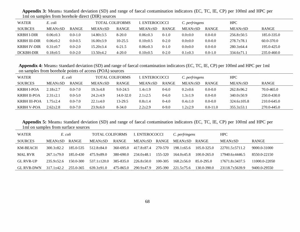
68
Appendix 3: Means± Standard deviation (SD) and range of faecal contamination indicators (EC, TC, IE, CP) per 100ml and HPC per
1ml on samples from borehole direct (DIR) sources
WATER E. coli TOTAL COLIFORMS I. ENTEROCOCCI C. perfringens HPC
SOURCES MEAN±SD RANGE MEAN±SD RANGE MEAN±SD RANGE MEAN±SD RANGE MEAN±SD RANGE
KRBH I-DIR 0.06±0.3 0.0-1.0 14.80±3.5 8-20.0 0.06±0.3 0-1.0 0.0±0.0 0.0-0.0 256.8±50.5 185.0-335.0
KRBH III-DIR 0.06±0.2 0.0-0.5 16.00±3.9 10-25.5 0.10±0.5 0-2.0 0.0±0.0 0.0-0.0 278.7±78.1 60.0-370.0
KRBH IV-DIR 0.31±0.7 0.0-2.0 15.20±3.4 6-21.5 0.06±0.3 0-1.0 0.0±0.0 0.0-0.0 280.3±64.4 195.0-425.0
DCKBH-DIR 0.18±0.5 0.0-2.0 13.50±4.2 4-20.0 0.10±0.5 0-2.0 0.1±0.3 0.0-1.0 334.6±71.1 235.0-460.0
Appendix 4: Means± Standard deviation (SD) and range of faecal contamination indicators (EC, TC, IE, CP) per 100ml and HPC per 1ml
on samples from borehole points of access (POA) sources
WATER E. coli TOTAL COLIFORMS I. ENTEROCOCCI C. perfringens HPC
SOURCES MEAN±SD RANGE MEAN±SD RANGE MEAN±SD RANGE MEAN±SD RANGE MEAN±SD RANGE
KRBH I-POA 2.18±2.7 0.0-7.0 19.3±4.8 9.0-24.5 1.4±1.9 0-6.0 0.2±0.6 0.0-0.0 262.8±96.2 70.0-465.0
KRBH II-POA 2.31±2.1 0.0-5.0 24.2±4.9 14.0-32.0 2.1±2.5 0-6.0 1.3±1.9 0.0-0.0 340.0±50.9 250.0-430.0
KRBH III-POA 1.75±2.4 0.0-7.0 22.1±4.0 13-29.5 0.8±1.4 0-4.0 0.4±1.0 0.0-0.0 324.6±105.8 210.0-645.0
KRBH V-POA 2.62±2.8 0.0-7.0 23.9±6.0 8-34.0 2.2±2.9 0-9.0 1.2±2.9 0.0-11.0 355.3±53.1 270.0-445.0
Appendix 5: Means± Standard deviation (SD) and range of faecal contamination indicators (EC, TC, IE, CP) per 100ml and HPC per
1ml on samples from surface sources
WATER E. coli TOTAL COLIFORMS I. ENTEROCOCCI C. perfringens HPC
SOURCES MEAN±SD RANGE MEAN±SD RANGE MEAN±SD RANGE MEAN±SD RANGE MEAN±SD RANGE
KM-BEACH 300.3±82.2 185.0-535 512.8±84.0 360-695.0 417.8±87.4 270-570 198.1±65.6 105.0-325.0 22701.5±5711.2 9000.0-31000
MAL RVR 267.1±79.0 185.0-430 475.9±89.0 380-690.0 234.0±48.1 155-320 164.0±45.8 100.0-265.0 17940.6±4446.5 8550.0-22150
GL RVR-UP 235.9±52.6 150.0-300 537.1±120.0 385-835.0 226.8±50.0 100-305 168.2±56.0 85.0-295.0 17671.8±3437.5 11000.0-22050
GL RVR-DWN 317.1±42.2 255.0-365 639.3±91.0 475-865.0 290.9±47.9 205-390 221.5±75.6 130.0-390.0 23118.7±5639.9 9400.0-29550