Embed Size (px)
Citation preview

Organisation for Economic Co-operation and Development 2003 Organisation de Coopération et de Développement Economiques
ENV/EPOC/GSP(2002)12/FINAL
WORKING PARTY ON GLOBAL AND STRUCTURAL POLICIES
OECD Workshop on the Benefits of Climate Policy: Improving Information for Policy Makers
Background Paper: Estimating Global Impacts from
Climate Change
by
Joel Smith and Sam Hitz

Copyright OECD, 2003
Application for permission to reproduce or translate all or part of this material should be addressed to the Head of Publications Services, OECD, 2 rue André Pascal, 75775 Paris, Cedex 16, France

FOREWORD
This paper was prepared for an OECD Workshop on the Benefits of Climate Policy: Improving Information for Policy Makers, held 12-13 December 2002. The aim of the Workshop and the underlying Project is to outline a conceptual framework to estimate the benefits of climate change policies, and to help organise information on this topic for policy makers. The Workshop covered both adaptation and mitigation policies, and related to different spatial and temporal scales for decision-making. However, particular emphasis was placed on understanding global benefits at different levels of mitigation -- in other words, on the incremental benefit of going from one level of climate change to another. Participants were also asked to identify gaps in existing information and to recommend areas for improvement, including topics requiring further policy-related research and testing. The Workshop brought representatives from governments together with researchers from a range of disciplines to address these issues. Further background on the workshop, its agenda and participants, can be found on the internet at: www.oecd.org/env/cc
The overall Project is overseen by the OECD Working Party on Global and Structural Policy (Environment Policy Committee). The Secretariat would like to thank the governments of Canada, Germany and the United States for providing extra-budgetary financial support for the work.
This paper is issued as an authored “working paper” -- one of a series emerging from the Project. The ideas expressed in the paper are those of the author alone and do not necessarily represent the views of the OECD or its Member Countries.
As a working paper, this document has received only limited peer review. Some authors will be further refining their papers, either to eventually appear in the peer-reviewed academic literature, or to become part of a forthcoming OECD publication on this Project. The objective of placing these papers on the internet at this stage is to widely disseminate the ideas contained in them, with a view toward facilitating the review process.
Any comments on the paper may be sent directly to the authors at:
Joel Smith and Sam Hitz Stratus Consulting Inc., Boulder, CO, USA E-mail: [email protected] and [email protected]
Comments or suggestions concerning the broader OECD Project may be sent to the Project Manager:
Jan Corfee Morlot at: [email protected]

TABLE OF CONTENTS
FOREWORD.................................................................................................................................................. 3
EXECUTIVE SUMMARY ............................................................................................................................ 6
1. INTRODUCTION ............................................................................................................................. 10
2. AGRICULTURE ............................................................................................................................... 24
3. SEA LEVEL RISE............................................................................................................................. 38
4. WATER RESOURCES ..................................................................................................................... 45
5. HUMAN HEALTH ........................................................................................................................... 53
6. TERRESTRIAL ECOSYSTEMS PRODUCTIVITY ....................................................................... 62
7. FORESTRY....................................................................................................................................... 67
8. MARINE ECOSYSTEM PRODUCTIVITY..................................................................................... 71
9. BIODIVERSITY ............................................................................................................................... 73
10. ENERGY ........................................................................................................................................... 76
11. AGGREGATE ................................................................................................................................... 78
12. DISCUSSION.................................................................................................................................... 84
13. CONCLUSIONS ............................................................................................................................... 94
REFERENCES ............................................................................................................................................. 96

Tables
Table 1. Summary of global impacts studies .................................................................................. 14 Table 2. Summary matrix of sectors sensitive to climate change and key factors considered in
existing studies.................................................................................................................. 22 Table 3. Temperature and precipitation forecasts for Rosenzweig et al. (1995) general circulation
models............................................................................................................................... 25 Table 4. Temperature, precipitation, and CO2 forecasts for Parry et al. (1999) general circulation
models............................................................................................................................... 26 Table 5. Socioeconomic baseline assumptions in Parry et al. (1999)............................................. 29 Table 6. Water use scenarios .......................................................................................................... 47 Table 7. Annual impact of a 1ºC increase in GMT - change in Gross Domestic Product .............. 79 Table 8. Summary of sectoral damage relationships with increasing temperature......................... 85
Figures
Figure 1. Responses of temperature to increasing CO2 concentrations and correlations between temperature increase and precipitation change ................................................................. 27
Figure 2. Temperature versus percent change in number of people at risk for hunger (2060) ........ 31 Figure 3. Percentage change in agricultural production as a function of temperature ..................... 32 Figure 4. Percentage change in number of people at risk of hunger as a function of temperature .. 33 Figure 5. Increase in number of people at risk of hunger due to climate change in the 2080s ........ 34 Figure 6. Costs of sea level rise in OECD countries ........................................................................ 41 Figure 7. Additional people in the hazard zone as a function of sea level rise ................................ 41 Figure 8. Additional average annual people flooded as a function of sea level rise ........................ 42 Figure 9. Additional people to respond due to sea level rise as a function of temperature.............. 42 Figure 10. Change in number of people in countries using more than 20% of their water resources as
a function of temperature.................................................................................................. 49 Figure 11. Difference between total population in countries where water stress increases and
countries where water stress decreases ............................................................................. 49 Figure 12. Percentage change in extent of potential malaria transmission as a function of
temperature ....................................................................................................................... 56 Figure 13. Additional people at risk for malaria (P. falciparum) as a function of temperature ......... 57 Figure 14. Additional people at risk for malaria (P. vivax) as a function of temperature.................. 57 Figure 15. Increase in diarrhoeal incidence ....................................................................................... 60 Figure 16. Change in global NPP (petagram) as a function of temperature....................................... 64 Figure 17. Change in global NEP (petagram/year) as a function of temperature .............................. 65 Figure 18. Change in global carbon (petagram) as a function of temperature ................................... 65 Figure 19. Percentage change in timber production for three 50-year time periods .......................... 69 Figure 20. Percent change in ecoclimatic classes for biosphere reserves compared to global
average.............................................................................................................................. 75 Figure 21. Idealised annual energy demand versus mean temperature .............................................. 77 Figure 22. Regional damage functions............................................................................................... 80 Figure 23. Global impacts in different sectors and according to method of aggregation................... 81 Figure 24. Estimated aggregate global damages ................................................................................ 82

EXECUTIVE SUMMARY
In addressing the consequences of greenhouse gas emissions, an important question is how the marginal benefits, or avoided damages, associated with controlling climate change vary with particular levels of mitigation. In other words, as more stringent levels of mitigation are reached, are there increasing benefits in terms of avoided damages from climate change? A few studies have attempted to answer this question by using a common metric, typically dollars, to express all impacts from climate change. (There are other ways to estimate marginal impacts, including identifying unique and vulnerable systems threatened by climate change, examining risk from extreme weather events, and identifying thresholds for triggering state changes in the global climate system, such as shutdown of thermohaline circulation.) While studies that aggregate impacts from climate change in terms of a single metric provide useful insight about how marginal impacts change, especially at higher levels of climate change, there are a number of concerns with such studies. One is that the common metric, particularly if it is dollars, may be difficult to apply to sectors that involve services that are not traded in markets and can also undervalue impacts in developing countries. A second is that it may actually be more useful for policy purposes to express results sector by sector, rather than as a single aggregate, and to highlight the distribution of these impacts.
This study therefore surveyed the literature on global impacts of climate change in specific sectors. It focused on the literature that examined global impacts up to 2100 and to a limited extent delineated some regional impacts as well. It did not attempt to summarize the regional impact literature. We used the metrics as reported in these studies, such as number of people affected, production, and primary productivity, as indicators of global impacts. We used change in global mean temperature (GMT) as the primary indicator of climate change, recognising that climate change is far more complex than this. For example, potential changes in regional climate and climate variance associated with a particular change in GMT can vary widely and encompass not only changes in temperature but also changes in precipitation and other climatic variables. We examined different studies to see if they showed a consistent relationship between impacts and increases in GMT. In particular, we tried to determine whether damages rise monotonically with increasing GMT, whether there are thresholds below which there are virtually no impacts, or whether there is a parabolic relationship, i.e., positive impacts followed by a reversal in sign.
The following categories were examined:
� agriculture
� sea level rise
� water resources
� human health
� terrestrial ecosystems productivity
� forestry
� marine ecosystems productivity

� biodiversity
� energy.
As far as we can discern, there are no published studies investigating global recreation and tourism, human amenity values, or migration, although these sectors will most likely experience impacts.
The results of our analysis are displayed in Table S-1.
Table S-1 Summary of sectoral damage relationships with increasing temperature
Sector Increasing adverse
impactsa Parabolic Unknown
Agriculture X
Coastal X
Water X
Health Xb
Terrestrial ecosystem productivity
X
Forestry X?c
Marine ecosystems X?d
Biodiversity X
Energy X
Aggregate X
a. Increasing adverse impacts means there are adverse impacts with small increases in GMT, and the adverse impacts increase with higher GMTs. We are unable to determine whether the adverse impacts increase linearly or exponentially with GMT. b. There is some uncertainty associated with this characterisation, as the results for the studies we examine are inconsistent. On balance, we believe the literature shows increasing damages for this sector c. We believe this is parabolic, but with only one study it is difficult to ascertain temperature relationship, so there is uncertainty about this relationship. d. This relationship is uncertain because there is only one study on this topic.
We found that the studies of coastal resources, marine ecosystems, human health, and biodiversity estimated increasing adverse impacts with higher GMT (although there are inconsistencies in the results for human health and limited data within the marine ecosystems sector). Agriculture, terrestrial ecosystem productivity, and forestry display a parabolic relationship (although the analysis of the forestry sector is limited). The current literature is inadequate to enable us to determine then nature of the relationship between GMT and impacts for the water and energy sectors. (There are global studies on water, but given the complexity of this sector, the results are inconclusive.) Finally, aggregate studies do not show a consistent relationship with GMT, so we label them as uncertain.
The studies we surveyed show that marginal adverse impacts increase in almost all of the sectors beyond an increase in GMT of 3 to 4°C. Below that range, the studies reach different conclusions. Many

show increasing adverse impacts, some show small impacts, and some show benefits for a few degree increase in GMT, which become adverse impacts by 3 to 4°C. The studies find adverse impacts at a few degrees of warming in several sectors (i.e., biodiversity and coastal resources). In addition, there could be adverse impacts for low levels of warming in health and marine productivity. While there may be adverse impacts in certain sectors with low levels of warming, the aggregate impacts below 3 to 4°C are uncertain.
Taken together, the studies suggest significant variation of impacts at the regional scale. Regional results may differ in magnitude and even sign from global ones. The nature of the relationship between change in temperature and impacts can be quite different at the regional scale. Some regions may experience net adverse aggregate impacts with warming of less than 3 to 4°C. Generally, lower latitude and developing countries face more negative effects than higher latitude and developed countries. Even within developing countries, there can be some sectors or regions that have benefits, while others have damages. There are exceptions to this pattern, one being biodiversity, where high latitude areas are at substantial risk of losing diversity.
The finding that global adverse impacts consistently increase beyond 3 to 4°C should be treated with caution for a number of reasons, including the following:
� Some key sectors are not included. As mentioned above, tourism and recreation, amenity values, and migration are not assessed. Also, we are uncertain about the relationship in some critical sectors such as water and health.
� Change in climate variance is generally not considered. Changes in climate variance and extreme events are, for the most part, not considered in the surveyed literature. Increased variance, including increased frequency and intensity of extreme events, could result in adverse effects at lower GMTs.
� Long-term impacts of climate change are not considered. The studies do not examine the consequences of climate change beyond 2100. Stabilising concentrations of greenhouse gas emissions in the 21st century will still result in further climate change in subsequent centuries, in particular sea level rise. In addition, climate change in the 21st century could trigger important changes in the climate system after 2100, such as slowdown or shutdown of the thermohaline circulation or disintegration of the West Antarctic ice sheet.
� Adaptation is often considered in a simple and inconsistent manner. We expect human adaptation to be complex. Studies of global impacts often make simple assumptions concerning adaptation, either assuming it is limited or assuming it is implemented with perfect efficiency. The truth probably lies somewhere between these two extremes. Also, because the studies quite often rely on different assumptions about adaptation, it is difficult to compare projections in a straightforward manner.
� Development is not examined in a consistent fashion. Development can substantially reduce vulnerability of societal sectors (e.g., agriculture, water resources, public health), but it can also increase vulnerability in some ways by increasing exposure. The studies we examined do not make standardised assumptions about development or about socioeconomic change in general.
� Sectoral interactions. The studies we considered tend to examine sectors in isolation. Interactions among sectors, such as changes in water supplies affecting agriculture, are generally not considered. These sorts of interactions could result in adverse impacts appearing at a lower GMTs than might otherwise be predicted.

Other important factors such as the effect of proactive adaptations in reducing vulnerability or the magnitude of ancillary benefits (e.g., reductions in pollution from greenhouse gas emission control measures) were also not considered in this study.
Finally, if results were converted to a common metric, it is possible that the total impacts would be negative at less than a 3 to 4°C increase in GMT.
Research should be devoted to address the lack of coverage of sensitive sectors, the inability to characterise the relationship between GMT and impacts, and inadequate consideration of key factors that can substantially affect that relationship between GMT and impacts.

1. INTRODUCTION
The Intergovernmental Panel on Climate Change (IPCC) concluded that the costs of stabilising greenhouse gas concentrations will rise gradually as mitigation efforts move atmospheric concentrations of carbon dioxide (CO2) from 650 ppm to 550 ppm and will rise more sharply as concentrations decrease further, from 550 ppm to 450 ppm (Metz et al., 2001). An important question is how the marginal benefits, or avoided damages, associated with controlling climate vary with particular levels of mitigation. In other words, what are the (presumed) benefits or avoided damages of reducing atmospheric concentrations of greenhouse gases to progressively lower levels?1
Some studies have attempted to address this question. Smith et al. (2001) identified approximate climate thresholds beyond which globally adverse impacts might emerge, but did not identify how marginal damages or benefits might vary with changing climate. A number of studies have attempted to quantify benefits of stabilising climate change (e.g., Fankhauser, 1995; Tol, 2002a; Nordhaus and Boyer, 2000), typically expressing benefits in terms of a common metric, often dollars. For the most part, they surveyed the literature and used expert judgement to develop algorithms expressing the relationship between climate change (typically measured in terms of change in global mean temperature) and impacts. The impacts are generally monetized, which allows for direct comparison of the benefits of controlling climate to greenhouse gas emission control costs.
However, one of the chief problems of such an approach is the choice of a common metric. While dollars may be an appropriate unit for quantifying impacts to market systems such as agriculture or forestry, they may not be as appropriate for enumerating impacts to other sectors. In addition, relying on a metric like dollars weighs impacts to those with greater financial resources more than impacts to those with fewer financial resources. Other numeraires such as number of people affected or change in land use or classification are common choices, but they also have limitations. For instance, tallying the number of people affected does not account for the degree to which they are affected or the type of risk they might face and it can lead to double counting. Nor is it always clear whether winners, those who somehow benefit from climate change, should offset those who stand to lose in aggregation. Similarly, change in land use or classification does not measure degree of impact and can allow for double counting as well.
In this study, we attempt to identify the marginal benefits associated with different levels of climate change. We do so based on a survey of primarily sectoral studies that have attempted to quantify global impacts of climate change. Instead of converting impacts to a common metric such as dollars, we retain the different metrics reported by the authors. Clearly, this prohibits us from aggregating our results across sectors. Our goal is not to develop a single estimate of global benefits across sectors. Rather, it is to examine the relationships between climate change and impacts in particular sectors and see if general patterns emerge.
It should be noted that a comprehensive examination of the impacts of climate change, whether by sector or in aggregate, is not the only way to identify important marginal impacts of climate change. Smith et al. (2001) identified five “reasons for concern.” Aggregate impacts, which are addressed in this
1. See Questions 3 and 6 in the IPCC Synthesis Report (Watson and the Core Writing Team, 2001).

paper, and distributional impacts, which are addressed to some extent, are two of the “reasons for concern.” The other three are risks to unique and threatened systems (i.e., loss or extensive damage to a valuable system), risks arising from increased extreme weather events, and risks of triggering large-scale singular events such as breakup of the West Antarctic Ice Sheet. These last three “reasons for concern” are not addressed in this paper. To our knowledge there are no global impact studies that focus on any of these three.
The matter of what index to use to measure levels of climate change is also a challenging one. There is an extensive discussion of this issue in Smith et al. (2001). Ideally, greenhouse gas emissions or atmospheric concentrations thereof would be the index of choice. This is because the use of either would allow a relatively direct comparison of the benefits associated with controlling climate to the costs associated with a particular level of mitigation effort. The problem with these metrics is that there is a range of uncertainty about how climate will change given any rate of emissions or concentration (indeed, there is uncertainty regarding the atmospheric concentration that will develop from a particular emissions rate; see Box 19-1 in Smith et al.).
We use global mean temperature (GMT) as the index for measuring the global mean climate change associated with impacts detailed in the studies we review. Certainly, for any change in GMT there are a range of concomitant changes in global precipitation and other meteorological variables. Global precipitation rises as mean temperature rises because the hydrological cycle is enhanced. A wide range of potential regional patterns of climate change are also associated with a particular change in GMT. Variation in these regional patterns can have a profound effect on regional impacts and even net global impacts. Thus, one would expect an examination of the type we undertake to yield a wide range of potential impacts for any given GMT. We use GMT because it is the most feasible index of climate change, but note its limitations. The analysis is focused primarily on elucidating global impacts. Regional impacts are discussed in only limited fashion, in order to highlight the point that they often differ substantially from global impacts. This report does not paint a comprehensive picture of impacts at the regional level.
A critical first step of characterising the relationship between climate change and pursuant impacts is determining the general shape of the damage curve, which quantitatively defines this relationship. For instance, do impacts appear with a small amount of warming and increase with higher levels of warming? If so, do the impacts increase linearly (the same increase in impacts for each degree warming) or exponentially (following a concave path, i.e., increasing impacts for each successive degree of warming), or do they stabilise at a particular level (increase asymptotically, i.e., decreasing additional impacts for each successive degree of warming)? Are there thresholds below which there are no impacts and beyond which there are impacts? The last relationship would suggest that small levels of climate change might have virtually no important impacts. Or, is the relationship between impacts and climate change parabolic, such that at lower levels of climate change, there might be benefits, beyond some point benefits start to decrease and eventually, at high enough levels of climate change, there are impacts?2 These questions are important because their answers determine whether there are benefits associated with lower GMT and whether those benefits remain constant, decrease, or increase as GMT rises. Actually elucidating this relationship is not always straightforward given the few data points that most studies provide. In these cases, we rely on knowledge of the underlying biophysical relationships to bolster our conclusions regarding the shapes of damage curves.
2. Linear damages can be expressed as (Y = kX; where Y is damages, X is temperature and k is a constant);
exponential damages as (Y = kXn; where n is a growth constant); stabilizing damages as (Y = log kX); threshold damages as (Y = 0 if X < N; Y = kX if X > N; where N is a specific temperature); and parabolic damages as (Y = -kX + mXn; where m is a constant).

This paper reviews published studies that estimate global impacts of climate change for sensitive sectors. The following categories are examined:
� agriculture
� sea level rise
� water resources
� human health
� terrestrial ecosystems productivity
� forestry
� marine ecosystems productivity
� biodiversity
� energy.
As far as we can discern, there are no published studies investigating global recreation and tourism, although these sectors will most likely experience impacts. Some limited studies on this sector suggest while tourists are responsive to temperatures, they are unlikely to be negatively affected by climate change. Tourists may simply substitute one destination for another or one travel date for another (Lise and Tol, 2002). However, this should not obscure the fact that local and regional impacts could be substantial. We also examined recent studies that attempt to estimate aggregate impacts (cross sectoral) on a global scale.
We surveyed the literature to assess whether the published studies are thorough and credible enough to enable us to estimate marginal changes in global impacts across the range of likely GMT changes for the 21st century. We also examined the studies in light of the following elements:
� Choice of metric. We report what metric each study uses to measure the impacts of climate change in the particular sector or sectors it addresses. We briefly discuss the advantages and disadvantages of the various metrics.
� Scenarios of climate change examined. Houghton et al. (2001) concluded that GMT could increase by 1.4 to 5.8°C above 1990 levels by 2100.3 Do studies individually or conjunctively address this wide a range of change in GMT? As we have already suggested, even for a specific change in GMT, there is a wide range of possible changes in regional climates and variance that can substantially affect a study’s results or the interpretation of these results. We also consider whether changes in extreme events or other changes in climate variance are analysed. Rate of climate change is also important, and we assess whether the studies considered it.
� Time frame. We summarise the time periods considered in each study. Do the studies correspond to a single point in time or do they cover a period of time in dynamic fashion? The time frame is important for a number of reasons. If baseline socioeconomic changes are
3. Even this range published by the IPCC may not represent the potential range of climate change in the 21st
century. IPCC also reports that the range of increase in GMT caused by a doubling of CO2 in the atmosphere is 1.5 to 4.5°C (Cubasch et al., 2001). However, Forest et al. (2002) concluded that the 90% confidence range for CO2 doubling is 1.4 to 7.7°C. This implies that the range of possible warming is larger than that reported by IPCC.

considered, then choice of time frame can affect results. Choice of time frame can also determine the rapidity of climate change the study considers.
� Key factors. Do the studies appropriately account for key factors that can substantially influence results, and even reverse the sign of a result? Among the key factors are adaptation, socioeconomic changes (baseline changes), and assumptions concerning biophysical processes such as carbon dioxide fertilisation of vegetation. Studies that do not consider one or more of these factors may have a substantial bias. Studies sometimes assume a greater role or influence of these factors than may actually be realised. Some studies may assume a larger carbon dioxide fertilisation effect than may occur in field conditions, while other studies may assume more effective adaptation than may actually happen.
� Spatial scale and distribution. We examine what spatial scales are used in the studies. Although the studies estimate global impacts, almost all of them estimate impacts at a regional scale, which are then summed to arrive at global numbers. In many instances, calculation of regional impacts in turn relies on the summation of local results. How disaggregated then are the regional results for any given study? Furthermore, what broad brush regional patterns emerge? In particular, how do results differ by latitude, continent, or level of development? Typically, discussion of regional results does not address distribution of impacts within regions or societies. So, for example, the relative effects on the poor versus the rich are seldom addressed.
� Results. Finally, for each topic, we discuss the results. We are mainly interested in the estimates each study derived of the quantitative relationship between climate change and impacts. Do they demonstrate a steady increase or decrease of impacts, are there thresholds, or are there reversals in sign, e.g., benefits at low levels of GMT and damages at higher levels? Where there is more than one study for a topic, are the results consistent?
We address each topic in turn. The results are summarised in Table 1 as well as in figures throughout the paper. Table 2 presents a comprehensive list of sectors that are likely to be sensitive to climate change, not simply those for which studies exist. It characterises existing studies within these sectors according to a number of key factors, and so provides a simple overview of the studies we examined. We also examined the literature on aggregate impacts.
Finally, the paper discusses the conclusions that can be drawn about impacts on the whole, the uncertainties surrounding such conclusions, and several related topics. Finally, we present some suggestions for future research to reduce uncertainties.

14
Tab
le 1
. S
um
mar
y o
f g
lob
al im
pac
ts s
tud
ies
Sect
or
Met
ric
Dri
ving
sc
enar
io(s
) T
ime
fram
e(s)
T
emp.
leve
l(s
Spat
ial s
cale
/ di
stri
buti
onal
K
ey f
acto
rs (
adap
tati
on,
base
line
chan
ge, C
O2 f
ert.)
Cha
nge
in
extr
eme
even
ts
or v
aria
nce
cons
ider
ed?
Stat
e ch
ange
s or
ra
tes
of c
hang
e ex
amin
ed?
Res
ults
Agr
icul
ture
R
osen
zwei
g et
al
., 19
95
No.
of
pe
ople
at
ri
sk
of
hung
er.
Cer
eal
prod
uctio
n Fo
od p
rice
s.
2xC
O2
for
3 G
CM
s B
asel
ine
clim
atol
ogy
1951
-198
0
2060
eq
uilib
rium
G
ISS4
.2°C
G
FDL
4.0°
C
UK
MO
5.2°
C
GIS
S-A
2.4
°C
Nat
iona
l;.
18 c
ount
ries
. 2
degr
ees
of
farm
le
vel
adap
tati
on +
wor
ld e
cono
mic
ad
just
men
ts
+
CO
2 ef
fect
+
in
crea
sing
yi
elds
+
ev
olvi
ng
base
line.
Not
cap
ture
d N
ot c
aptu
red
Figu
re 1
Dar
win
et
al.,
19
95
%
chan
ge
in
prod
uctio
n of
ag
ricu
ltura
l co
mm
oditi
es
base
d on
lan
d-us
e ch
ange
.
2x
CO
2 fo
r 4
GC
Ms
Bas
elin
e cl
imat
olog
y 19
51-1
980
2090
eq
uilib
rium
G
ISS
4.2°
C
GFD
L 4
.0°C
U
KM
O 5
.2°C
O
SU 2
.8°C
Reg
iona
l —
maj
or
coun
trie
s pl
us
geog
raph
ic r
egio
ns.
Farm
lev
el a
dapt
atio
n, n
o C
O2
effe
ct,
no
evol
ving
ba
selin
e.
1990
wor
ld a
s be
nchm
ark.
Not
cap
ture
d N
ot c
aptu
red
Figu
re 2
Parr
y et
al
., 19
99
No.
of
peop
le
at r
isk
of
hung
er.
Food
pr
oduc
tion.
Fo
od p
rice
s.
Tra
nsie
nt
GC
M
scen
ario
s B
asel
ine
clim
atol
ogy
1961
-199
0
2020
s,
2050
s,
2080
s H
adC
M2
1.2-
3.1°
C
Had
CM
3 1.
1- 3
.0°C
R
egio
nal;
dist
ribu
tion
al
effe
cts
cons
ider
ed.
Farm
lev
el a
dapt
atio
n +
wor
ld
econ
omic
ad
just
men
ts
+ in
crea
sing
yi
elds
du
e to
te
chno
logy
.
Not
cap
ture
d T
rans
ient
. R
esul
ts
at
2020
s,
2050
s,
2080
s pr
ovid
e so
me
insi
ght
into
ra
tes
of c
hang
e
Figu
re 3
Fisc
her
et a
l.,
2002
Pr
oduc
tion
po
tent
ial,
GD
P of
ag
ricu
lture
, co
nsum
ptio
n,
no. o
f pe
ople
at
risk
of
hung
er.
Var
ious
SR
ES
scen
ario
s fo
r 4
GC
Ms
2080
s D
epen
dent
on
part
icul
ar
scen
ario
an
d G
CM
. Sc
enar
ios
cove
r up
to
6°
C.
Reg
iona
l Fa
rm le
vel a
dapt
atio
n. N
o C
O2
effe
ct.
Not
cap
ture
d N
ot c
aptu
red
Figu
re 4
Sea
leve
l/coa
stal
Fa
nkha
user
, 19
95
Dir
ect
cost
(c
ost
of
prot
ecti
on,
dryl
and
loss
an
d w
etla
nd
loss
) m
easu
red
in $
Var
ious
in
crem
ents
of
se
a le
vel
rise
(S
LR
) re
lati
ve t
o 19
90
2100
N
ot
appl
icab
le.
SL
R
rise
up
to 2
00 c
m
OE
CD
Cou
ntri
es
Zer
o ut
ility
di
scou
ntin
g,
Opt
imal
co
asta
l pr
otec
tion
co
nsid
ered
bu
t as
pr
otec
t or
re
trea
t dic
hoto
my.
No
chan
ge
in
stor
min
ess
Not
cap
ture
d Fi
gure
5.
Wet
land
da
mag
es
dom
inat
e.

15
Tab
le 1
. Su
mm
ary
of
glo
bal
imp
acts
stu
die
s (c
on
t.)
Sect
or
Met
ric
Dri
ving
sc
enar
io(s
) T
ime
fram
e(s)
T
emp.
leve
l(s)
Sp
atia
l sca
le /
dist
ribu
tion
al
Key
fac
tors
(ad
apta
tion
, ba
selin
e ch
ange
, CO
2 fer
t.)
Cha
nge
in
extr
eme
even
ts
or v
aria
nce
cons
ider
ed?
Stat
e ch
ange
s or
ra
tes
of c
hang
e ex
amin
ed?
Res
ults
Sea
leve
l/coa
stal
con
t.
Nic
holls
et a
l.,
1999
N
o. o
f pe
ople
at
ris
k of
co
asta
l fl
oodi
ng
Tra
nsie
nt G
CM
sc
enar
ios
SL
R r
elat
ive
to
1961
-199
0
2020
s, 2
050s
, 20
80s
Had
CM
2 1.
2-3.
1°C
H
adC
M3
1.1-
3.0°
C
SL
R o
f 12
, 24
and
40
cim
at 2
020s
, 205
0s
and
2080
s, r
espe
ctiv
ely
Sele
cted
reg
ions
an
d gl
obal
ag
greg
atio
n
Evo
lvin
g re
fer.
sce
nari
o +
impr
ovin
g fl
ood
defe
nce
stan
dard
s
No
chan
ges
in
stor
min
ess
cons
ider
ed.
Cur
rent
var
ianc
e im
pose
d on
sea
le
vel r
ise.
Not
cap
ture
d Fi
gure
s 6-
8.
Dar
win
and
T
ol, 2
002b
D
irec
t cos
t (c
aptu
res
cost
of
pro
tect
ion,
fi
xed
capi
tal
and
land
) +
eq
uiva
lent
va
riat
ion
(cap
ture
s se
cond
ary
econ
omic
ef
fect
s)
0.5
met
er li
near
ri
se in
sea
leve
l re
lati
ve to
199
0,
assu
mpt
ion
of
linea
rity
. Se
nsit
ivit
y an
alys
is o
f un
cert
aint
y in
en
dow
men
t va
lues
and
lim
itat
ion
of D
C
vs. E
V
2100
0.
5 m
SL
R
Reg
ions
Pu
re ti
me
rate
of
pref
eren
ce =
1%
+ e
cono
mic
ally
opt
imal
co
asta
l pro
tect
ion
+ 1
990
econ
omic
bas
elin
e bu
t in
crea
sing
land
val
ue
Not
cap
ture
d N
ot c
aptu
red
C
urre
nt
esti
mat
es o
f en
dow
men
t un
cert
aint
y le
ad
to 3
6%
diff
eren
ce in
DC
gl
obal
ly. E
V
loss
es 1
3%
high
er th
an D
Cs
glob
ally
. R
egio
nally
, can
be
up
to 1
0%
low
er th
ough
.

16
Tab
le 1
. Su
mm
ary
of
glo
bal
imp
acts
stu
die
s (c
on
t.)
Sect
or
Met
ric
Dri
ving
sc
enar
io(s
) T
ime
fram
e(s)
T
emp.
leve
l(s)
Sp
atia
l sc
ale/
di
stri
buti
onal
Key
fac
tors
(ad
apta
tion
, ba
selin
e ch
ange
, C
O2
fert
.)
Cha
nge
in e
xtre
me
even
ts
or
vari
ance
co
nsid
ered
?
Stat
e ch
ange
s or
ra
tes
of
chan
ge
exam
ined
? R
esul
ts
Wat
er
Arn
ell,
1999
N
o.
of
peop
le
livin
g in
co
untr
ies
expe
rien
cing
w
ater
str
ess
GC
Ms
4 H
adC
M2
scen
ario
s 1
Had
CM
3 sc
enar
io
Bas
elin
e cl
imat
olog
y 19
61-1
990
2020
s,
2050
s,
2080
s H
adC
M2
1.2-
3.1°
C
Had
CM
3 1.
1-3.
0°C
N
atio
nal
Dis
trib
utio
nal
diff
eren
ces
in
runo
ff e
xam
ined
at
regi
onal
leve
l
Dem
and
unaf
fect
ed
by
clim
ate
chan
ge
in
use
scen
ario
s.
Use
sc
enar
ios
inco
rpor
ated
ch
ange
s in
po
pula
tion
s,
effi
cien
cy,
irri
gatio
n,
indu
stry
, et
c.
Lan
d us
e w
ithi
n ea
ch
catc
hmen
t as
sum
ed
cons
tant
. N
o di
rect
C
O2
effe
ct.
Lim
ited
tre
atm
ent
of
10 y
r. m
ax.
mon
thly
ru
noff
and
10
yr. l
ow
annu
al to
tal r
unof
f.
Not
cap
ture
d Fi
gure
s 9-
10.
Vör
ösm
arty
et
al.,
2000
N
o.
of
peop
le
livin
g un
der
wat
er
stre
ssed
co
nditi
ons
Can
adia
n M
odel
C
GC
M1
Had
CM
2 B
asel
ine
clim
atol
ogy
1961
-199
0
2025
N
ot r
epor
ted
Riv
er s
yste
m le
vel
Est
imat
es o
f fu
ture
wat
er
effi
cien
cy
inco
rpor
ated
, ca
ptur
es
spat
ial
hete
roge
neit
y by
usi
ng 3
0’
grid
ce
lls.
Allo
wed
fo
r m
igra
tion
wit
hin
coun
trie
s to
sou
rces
of
wat
er.
Not
cap
ture
d
Not
cap
ture
d E
ffec
ts
of
incr
ease
d w
ater
de
man
d du
e to
po
pula
tion
an
d ec
onom
ic
grow
th
eclip
se
chan
ges
due
to
clim
ate.
So
me
regi
onal
da
mag
es
are
mas
ked
thou
gh
(e.g
., A
fric
a,
Sout
h A
mer
ica)
Döl
l, 20
02
Net
ir
riga
tion
requ
irem
ents
E
CH
AM
4/
OPY
C3
Had
CM
3AA
B
asel
ine
clim
atol
ogy
1961
-199
0
2020
s, 2
070s
N
ot r
epor
ted
0.5°
by
0.5°
ras
ter
cells
, re
gion
al
aggr
egat
ion
Allo
wed
fo
r ch
ange
s in
st
art
of
grow
ing
seas
on,
crop
ping
pat
tern
s. L
imit
ed
to 1
995
irri
gate
d ar
eas.
Com
pare
re
sults
to
va
rian
ce
of
past
ce
ntur
y.
Not
cap
ture
d R
egio
nal
anal
ysis
sh
ows
IR
requ
irem
ent
in
12/1
7 w
orld
re
gion
s in
crea
ses,
bu
t no
t m
ore
than
by
10%
A
lcam
o et
al.,
19
97
Num
ber
of
peop
le li
ving
in
wat
er
scar
ce
cond
ition
s
EC
HA
M4
and
GFD
L
2025
, 207
5 N
ot r
epor
ted
0.5�
by
0.
5�gr
id
leve
l, na
tion
al
aggr
egat
ion
Con
side
red
thre
e di
ffer
ent
scen
ario
s of
w
ater
us
e.
Wat
er
use
cons
ider
ed
cons
umpt
ive.
L
and
use
chan
ges
inco
rpor
ated
.
Lim
ited
tre
atm
ent
of
drou
ght
cycl
es,
but
no
chan
ge
in
vari
ance
pos
tula
ted.
Not
cap
ture
d W
ater
sc
arci
ty
decr
ease
s du
e to
cl
imat
e ch
ange
by
2075
.

17
Tab
le 1
. Su
mm
ary
of
glo
bal
imp
acts
stu
die
s (c
on
t.)
Sect
or
Met
ric
Dri
ving
sc
enar
io(s
) T
ime
fram
e(s)
T
emp.
leve
l(s)
Sp
atia
l sca
le/
dist
ribu
tion
al
Key
fac
tors
(a
dapt
atio
n, b
asel
ine
chan
ge, C
O2 f
ert.
)
Ext
rem
e ev
ents
or
vari
ance
co
nsid
ered
?
Stat
e ch
ange
s or
rat
es o
f ch
ange
ex
amin
ed?
Res
ults
Hea
lth
Mar
tin a
nd
Lef
ebvr
e, 1
995
Are
a of
pot
entia
l tr
ansm
issi
on
2XC
O2
GFD
LQ
, GIS
S,
OSU
, UK
MO
, G
FDL
B
asel
ine
clim
atol
ogy
1951
-19
80
Not
exp
licit
ly
stat
ed.
Pres
umab
ly
betw
een
2060
an
d 20
90.
GIS
S 4.
2°C
G
FDL
4.0
°C
UK
MO
5.2
°C
OSU
2.8
°C
30’
by 3
0’ g
rid
cells
N
o ep
idem
iolo
gy, n
o ad
apta
tion
, cru
de w
ater
ba
lanc
e as
sum
ptio
ns
Not
cap
ture
d N
ot c
aptu
red
Figu
re 1
1.
Mar
tens
et a
l.,
1999
N
o. o
f pe
ople
at
risk
of
mal
aria
H
adC
M2
Had
CM
3 B
asel
ine
clim
atol
ogy
1961
-19
90
2020
s, 2
050s
, 20
80s
Had
CM
2: 1
.2-3
.1°C
H
adC
M3:
1.1
-3.0
°C
Reg
iona
l E
volv
ing
pop.
bas
elin
e,
no a
dapt
atio
n, v
ecto
r’s
rang
e un
chan
ged
by
clim
ate
Not
cap
ture
d N
ot c
aptu
red
Figu
res
12-1
3.
Tol
and
D
owla
taba
di, 2
002
Vec
tor-
born
e m
orta
lity,
mal
aria
m
orta
lity
Var
. miti
gati
on
polic
ies
appl
ied
to
assu
med
mor
talit
y ti
me
rela
tion
ship
.
2100
T
emp.
mor
talit
y re
lati
onsh
ip h
ypot
hesi
sed
from
sev
eral
stu
dies
.
Reg
iona
l N
o ev
olut
ion
of c
ontr
ol
effo
rts,
acc
ess
to p
ublic
he
alth
ser
vice
ac
cord
ing
to in
com
e,
popu
lati
on in
reg
ions
ho
mog
enou
s, n
o la
nd
use
chan
ge e
ffec
ts
Not
cap
ture
d N
ot c
aptu
red
Glo
bal m
orta
lity
due
to m
alar
ia
redu
ced
to z
ero
by
2100
due
to
econ
omic
gro
wth
Hij
ioka
et a
l.,
2002
D
iarr
hoea
l in
cide
nce
Tem
pera
ture
sc
enar
ios
deri
ved
from
NIE
S/C
CSR
2025
, 205
5 0.
8-3.
4°C
R
egio
nal
Stat
istic
al m
odel
as
sum
es th
at w
ater
su
pply
cov
erag
e an
d te
mpe
ratu
re d
eter
min
e di
arrh
oeal
inci
denc
e in
fu
ture
. Acc
ess
to s
uppl
y im
prov
es w
ith
inco
me.
Not
cap
ture
d N
ot c
aptu
red
Figu
re 1
4

18
Tab
le 1
. Su
mm
ary
of
glo
bal
imp
acts
stu
die
s (c
on
t.)
Sect
or
Met
ric
Dri
ving
sc
enar
io(s
) T
ime
fram
e(s)
T
emp.
leve
l(s)
Sp
atia
l sca
le/
dist
ribu
tion
al
Key
fac
tors
(a
dapt
atio
n, b
asel
ine
chan
ge, C
O2 f
ert.
)
Cha
nge
in
extr
eme
even
ts o
r va
rian
ce
cons
ider
ed?
Stat
e ch
ange
s or
rat
es o
f ch
ange
ex
amin
ed?
Res
ults
Ter
rest
rial
eco
syst
ems
Whi
te e
t al.,
199
9 V
eget
atio
n ca
rbon
, soi
l ca
rbon
, NPP
, N
EP
4 H
adC
M2
sim
ulat
ions
, 1
Had
CM
3 si
mul
atio
n. IS
92a
forc
ing.
Inpu
t to
dyna
mic
veg
. m
odel
Hyb
rid
v4.1
1860
-210
0 1.
1�-3
.1� C
T
en 2
00m
2 plo
ts
per
GC
M g
rid
in
vege
tati
on m
odel
. R
esul
ts
aggr
egat
ed
glob
ally
Dis
pers
al p
roce
sses
not
re
pres
ente
d-po
tent
ial
vege
tati
on. L
and
use
and
dist
urba
nces
not
m
odel
led.
No
vege
tati
on-c
limat
e fe
edba
cks.
Nitr
ogen
de
posi
tion
exog
enou
s.
Stoc
hast
ic w
eath
er
gene
rato
r us
ed to
cr
eate
dai
ly
tem
pera
ture
s fo
r in
put i
nto
vege
tati
on m
odel
. N
o st
ate
chan
ge in
va
rian
ce m
odel
led.
Not
cap
ture
d Fi
gure
s 15
-16.
Cra
mer
et a
l.,
2001
N
PP, N
EP,
Soi
l C
, Bio
mas
s H
adC
M2-
SUL
w
ith
IS19
2a
forc
ing
inpu
t to
6 D
GV
Ms.
Sc
enar
ios
incl
ude:
1)
cha
ngin
g C
O2
2) c
hang
ing
clim
ate
with
CO
2 at
pre
indu
stri
al
3) c
hang
es in
cl
imat
e an
d C
O2
Bas
elin
e cl
imat
olog
y 19
31-
1960
2100
21
99 w
ith
100
year
s of
un
real
istic
im
pose
d eq
uilib
rium
st
artin
g at
210
0
Not
rep
orte
d as
glo
bal
mea
ns.
Fund
amen
tally
re
gion
al. G
loba
l co
vera
ge, b
ut
alm
ost n
o re
sults
ag
greg
ated
at a
gl
obal
leve
l
No
biog
eoch
em.
feed
back
s (e
.g.,
vege
tati
on to
cl
imat
e), a
s D
GV
Ms
are
run
offl
ine.
Lan
d us
e no
t inc
orpo
rate
d
Var
ianc
e in
GC
M
outp
ut m
aint
aine
d an
d in
put t
o D
VG
Ms,
but
no
stat
e ch
ange
in
vari
ance
co
nsid
ered
.
Not
cap
ture
d T
erre
stri
al c
arbo
n si
nk le
vels
off
by
2050
and
beg
ins
to d
ecre
ase,
by
end
of c
entu
ry

19
Tab
le 1
. Su
mm
ary
of
glo
bal
imp
acts
stu
die
s (c
on
t.)
Sect
or
Met
ric
Dri
ving
sc
enar
io(s
) T
ime
fram
e(s)
T
emp.
leve
l(s)
Sp
atia
l sca
le/
dist
ribu
tion
al
Key
fac
tors
(a
dapt
atio
n, b
asel
ine
chan
ge, C
O2 f
ert.
)
Cha
nge
in
extr
eme
even
ts o
r va
rian
ce
cons
ider
ed?
Stat
e ch
ange
s or
rat
es o
f ch
ange
ex
amin
ed?
Res
ults
For
estr
y So
hnge
n et
al.,
20
01
% c
hang
e in
fo
rest
are
a, N
PP,
tim
ber
yiel
d,
wel
fare
($)
2 eq
uilib
rium
sc
enar
ios
2xC
O2
Ham
burg
T-1
06
UIU
C
near
(19
95-
2045
) lo
ng (
2045
-21
45)
disc
ount
rat
es
of 3
, 5 a
nd 7
%
Equ
ilibr
ium
ac
hiev
ed b
y 20
60
Ham
burg
1°C
U
IUC
3.4
°C
Reg
iona
l C
O2
fert
., sp
ecie
s m
igra
tion
, lan
d us
e co
mpe
titio
n no
t m
odel
led
Not
cap
ture
d R
ate
of c
hang
e co
nsid
ered
to
exte
nt th
at
dieb
ack
scen
ario
in
vest
igat
ed a
s w
ell a
s re
gene
rati
on.
Figu
re 1
7. O
nly
two
tem
pera
ture
po
ints
, res
ults
for
w
hich
are
sim
ilar
glob
ally
. D
iffe
renc
es a
re
regi
onal
and
re
flec
t reg
iona
l te
mp.
dif
fere
nces
in
GC
M o
utpu
t. Pe
rez-
Gar
cia
et a
l., 1
997
NPP
, pri
ces,
w
elfa
re (
$)
4 eq
uilib
rium
sc
enar
ios,
2xC
O2
OSU
, GFD
L,
GFD
L-Q
, GIS
S B
asel
ine
clim
atol
ogy
1951
-19
80
Equ
ilibr
ium
as
sum
ed a
t 20
65, b
ut
resu
lts
pres
ente
d fo
r 20
40
OSU
: 2.8
°C
GFD
L: 3
.0°C
G
FDL
-Q: 4
.0°C
G
ISS:
4.2
°C
Not
rep
orte
d fo
r 20
40s,
w
hen
econ
omic
mod
el
ends
.
Reg
iona
l N
o dy
nam
ics
of s
peci
es
mig
rati
on o
r su
cces
sion
. “D
umb
Fore
ster
,” n
o ad
apti
ve m
anag
emen
t. 2
econ
omic
sce
nari
os:
Inte
nsiv
e an
d E
xten
sive
M
argi
n ha
rves
ting
Not
cap
ture
d N
ot c
aptu
red
Res
ults
do
not
vary
wid
ely
amon
g th
e fo
ur
GC
Ms,
esp
ecia
lly
at g
loba
l lev
el.
Pere
z-G
arci
a et
al.,
200
2 V
eget
atio
n ca
rbon
, sof
twoo
d an
d ha
rdw
ood
stoc
k, p
rice
, ha
rves
t, w
elfa
re
($)
Tra
nsie
nt c
hang
es
in C
O2.
3 sc
enar
ios
from
IG
CM
B
asel
ine
clim
atol
ogy
1850
-19
76
Stab
ilisa
tion
at
2100
, ana
lysi
s at
204
0
RR
R: 7
45pp
mv,
2.6
°C
HH
L: 9
36pp
mv,
3.1
°C
LL
H: 5
92pp
mv,
1.6
°C
Not
rep
orte
d fo
r 20
40
whe
n ec
onom
ic m
odel
en
ds
Reg
iona
l C
O2
fert
ilise
., re
vise
d ec
onom
. bas
elin
e in
clud
ing
Asi
an C
risi
s,
low
er R
ussi
an p
rod.
, no
spec
ies
mig
rati
on.
2 ha
rves
ting
scen
ario
s as
in
Per
ez-G
arci
a et
al.,
19
97
Not
cap
ture
d N
ot c
aptu
red
Nee
d tr
ansi
ent
tem
pera
ture
s.
Glo
bal p
rice
and
ha
rves
t cha
nges
ar
e sm
all.
Reg
iona
l cha
nges
ob
scur
ed th
ough
.

20
Tab
le 1
. Su
mm
ary
of
glo
bal
imp
acts
stu
die
s (c
on
t.)
Sect
or
Met
ric
Dri
ving
sc
enar
io(s
) T
ime
fram
e(s)
T
emp.
leve
l(s)
Sp
atia
l sca
le/
dist
ribu
tion
al
Key
fac
tors
(a
dapt
atio
n, b
asel
ine
chan
ge, C
O2 f
ert.
)
Cha
nge
in
extr
eme
even
ts o
r va
rian
ce
cons
ider
ed?
Stat
e ch
ange
s or
rat
es o
f ch
ange
ex
amin
ed?
Res
ults
Mar
ine
ecos
yste
ms
Bop
p et
al.,
200
1 C
hang
e in
mar
ine
expo
rt p
rodu
ctio
n 2
atm
/oce
an
coup
led
GC
Ms.
C
onst
ant C
O2 a
nd
1% g
row
th/y
r un
til 2
x af
ter
70 y
ears
. E
quili
briu
m f
or
3x a
nd 4
x C
O2.
Tw
o bi
ogeo
chem
ical
sc
hem
es.
70 y
ears
N
/A
Glo
bally
ag
greg
ated
. GC
M
grid
2�lo
ng
x1.5�la
t
Bio
geoc
hem
ical
sc
hem
es a
re p
hosp
hate
ba
sed,
lack
ing
limit
atio
n by
oth
er
nutr
ient
s (e
.g.,
Fe, N
, Si
)
Not
cap
ture
d N
ot c
aptu
red
Red
uctio
n of
6%
in
pro
duct
ion
for
2xC
O2
rela
tive
to
cont
rol.
11%
for
3x
and
15%
for
4x
Bio
dive
rsit
y/ s
peci
es lo
ss
Hal
pin,
199
7 %
Cha
nge
in
ecoc
limat
ic
clas
ses
in
bios
pher
e re
serv
es 2X
CO
2
GFD
L, G
ISS,
O
SU, U
KM
O
Bas
elin
e cl
imat
olog
y 19
51-
1980
Not
sta
ted
expl
icit
ly.
Pres
umab
ly
2060
-90,
as
wit
h ot
her
stud
ies
usin
g th
is b
atte
ry o
f m
odel
s.
GIS
S 4.
2°C
G
FDL
4.0
°C
UK
MO
5.2
°C
OSU
2.8
°C
Glo
bal
No
adap
tatio
n or
ba
selin
e ch
ange
s.
Not
cap
ture
d N
ot c
aptu
red
Figu
re 1
8
Ene
rgy
% c
hang
e in
GD
P FU
ND
22
00
Not
rep
orte
d fo
r dy
nam
ic
stud
y C
ount
ry s
peci
fic.
E
xtra
pola
ted
to
rest
of
the
wor
ld.
Incr
easi
ng e
ffic
ienc
y,
popu
lati
on, i
ncom
e N
ot c
aptu
red
Not
cap
ture
d Sa
ving
s du
e to
he
atin
g le
ss th
an
1% G
DP
by 2
200,
co
sts
due
to
cool
ing
abou
t 0.
6% G
DP.

21
Tab
le 1
. Su
mm
ary
of
glo
bal
imp
acts
stu
die
s (c
on
t.)
Sect
or
Met
ric
Dri
ving
sc
enar
io(s
) T
ime
fram
e(s)
T
emp.
leve
l(s)
Sp
atia
l sca
le/
dist
ribu
tion
al
Key
fac
tors
(a
dapt
atio
n, b
asel
ine
chan
ge, C
O2 f
ert.
)
Ext
rem
e ev
ents
or
vari
ance
co
nsid
ered
?
Stat
e ch
ange
s or
rat
es o
f ch
ange
ex
amin
ed?
Res
ults
Agg
rega
te
Tol
, 200
2a,b
In
com
e C
onsi
dere
d bo
th
1ºC
incr
ease
and
dy
nam
ic o
ver
two
cent
urie
s
2200
for
dy
nam
ic
1ºC
for
sta
tic, n
ot
repo
rted
for
dyn
amic
9
wor
ld r
egio
ns
Sect
or s
peci
fic
Not
cap
ture
d N
ot c
aptu
red
Sim
ple
sum
ag
greg
atio
n le
ads
to 2
.3%
incr
ease
in
glo
bal i
ncom
e N
ordh
aus
and
Boy
er, 2
000
Out
put
Reg
iona
l In
tegr
ated
mod
el
of C
limat
e an
d th
e E
cono
my
Not
rep
orte
d 2.
5ºC
, som
e re
sults
ex
trap
olat
ed to
6ºC
13
reg
ions
Se
ctor
spe
cifi
c N
o ca
ptur
ed
Cat
astr
ophi
c ev
ents
co
nsid
ered
1.5%
incr
ease
in
outp
ut w
eigh
ted
by in
com
e, 1
.9%
w
eigh
ted
by
popu
lati
ons.
Fi
gure
19.

22
Tab
le 2
. S
um
mar
y m
atri
x o
f se
cto
rs s
ensi
tive
to
clim
ate
chan
ge
and
key
fac
tors
co
nsi
der
ed in
exi
stin
g s
tud
ies
Ass
umpt
ions
T
ime
fram
e Im
pact
mod
e
CO
2 fe
rtili
sati
on
incl
uded
? A
dapt
atio
n in
corp
orat
ed?
Evo
lvin
g so
cio-
econ
omic
ba
selin
e?
2000
-20
50
2050
-21
00
Bey
ond
2100
Ext
rem
e ev
ents
ca
ptur
ed?
Stat
e ch
ange
s?
Tem
pera
ture
ra
nge
(°C
)
Agr
icul
ture
Ros
enzw
eig
et a
l.,
1995
X
X
X
X
X
2.4-
5.2
Dar
win
et a
l., 1
995
X
X
X
2.
8-5.
2 P
arry
et
al.,
1999
X
X
X
X
X
1.1-
3.1
Fis
cher
et
al.,
2002
X
X
X
X
up
to
6 Se
a le
vel
F
ankh
ause
r, 1
995
N/A
X
X
X
N
/A
Nic
holls
et
al.,
1999
N
/A
X
X
X
X
X
1.1-
3.1
Dar
win
and
Tol
, 20
02b
N/A
X
X
X
N
/A
Wat
er
A
rnel
l, 19
99
X
X
X
1.
1-3.
1 V
örös
mar
ty e
t al.,
20
00
X
X
X
N
/R
Alc
amo
et a
l., 1
997
X
X
X
N
/R
Döl
l, 20
02
X
X
X
X
N/R
W
ater
qua
lity
H
uman
hea
lth
M
arti
n an
d L
efeb
vre,
199
5 N
/A
X
X
2.
8-5.
2 M
arte
ns e
t al
., 19
99
N/A
X
X
X
1.
1-3.
1 H
ijio
ka e
t al.,
200
2 N
/A
X
X
X
0.8-
3.4
Tol
and
D
owla
taba
di, 2
002
N/A
X
X
X
N
/R

23
Tab
le 2
. Su
mm
ary
mat
rix
of
sect
ors
sen
siti
ve t
o c
limat
e ch
ang
e an
d k
ey f
acto
rs c
on
sid
ered
in e
xist
ing
stu
die
s (c
on
t.)
Ass
umpt
ions
T
ime
fram
e Im
pact
mod
e
CO
2 fe
rtili
sati
on
incl
uded
? A
dapt
atio
n in
corp
orat
ed?
Evo
lvin
g so
cio-
econ
omic
bas
elin
e?
2000
-20
50
2050
-21
00
Bey
ond
2100
Ext
rem
e ev
ents
ca
ptur
ed?
Stat
e ch
ange
s?
Tem
pera
ture
ra
nge
(°C
)
Ter
rest
rial
eco
syst
ems
W
hite
et
al.,
1999
X
N/A
X
X
1.1-
3.1
Cra
mer
et a
l., 2
001
X
N
/A
X
X
X
X
N
/R
For
estr
y
Sohn
gen
et a
l., 2
001
X
X
X
X
X
X
1-3.
4 P
erez
-Gar
cia
et a
l.,
1997
X
X
X
X
N
/R
Per
ez-G
arci
a et
al.,
20
02
X
X
X
X
N/R
M
arin
e ec
osys
tem
s
Bop
p et
al.,
200
1 N
/A
N
/A
X
X
N
/R
Bio
dive
rsit
y
Hal
pin,
199
7 N
/A
X
X
2.
8-4.
2 N
on m
arke
t ec
osys
tem
ser
vice
s
E
nerg
y
Tol
, 200
2b
N/A
X
X
X
X
N/R
T
rans
port
Bui
ldin
g
Rec
reat
ion
and
tour
ism
In
sura
nce
H
uman
am
enit
y
Mig
rati
on
N
otes
: N
/A =
not
app
licab
le, N
/R =
not
rep
orte
d.

24
2. AGRICULTURE
We examined four studies that investigated the possible effects of climate change on global agricultural production: Darwin et al. (1995), Rosenzweig et al. (1995), Parry et al. (1999), and Fischer et al. (2002). Parry et al. (1999) is part of a compendium of coordinated studies devoted to assessing the global effects of climate change, published as a Special Issue of Global Environmental Change.
Choice of metric
The four studies relied on a variety of indicators to examine climate change impacts on agricultural systems: food prices, production of particular crops, changes in potential agricultural land, overall production of agricultural commodities, and numbers of people at risk of hunger, among others. We focused primarily on the use of the last two measures, which incorporate the other measures.
Rosenzweig et al. (1995), Parry et al. (1999), and Fischer et al. (2002) generated estimates of the number of people at risk of hunger (defined as those with an income insufficient to either produce or procure their food requirements). There are several advantages to this sort of metric. First, it recognises that the effects of climate change may affect agricultural production through a variety of channels that are not simply biophysical. Production and the consequent supply of food depend on factors such as demand, price, and the nature of the world’s trade regimes. If ultimately what we are interested in is the ability of the world to feed its population, then it is a sensible numeraire. One additional advantage of this sort of metric is that it allows for cross-sectoral comparison to an extent. Numbers of people at risk of hunger because of impacts on agricultural systems can be weighed against number of people at risk of coastal flooding. However, the social and economic processes on which estimates of number of people at risk of hunger depend are complicated processes to model. Attempts to do so rely heavily on assumptions, for instance, about the future world population with respect to size, distribution, income, and level of development or about the degree of trade liberalisation. Results can be sensitive to these assumptions.
Darwin et al. (1995) and Fischer et al. (2002) also examined changes in the global production of agricultural commodities. In both studies, agriculture is considered in the context of a larger picture of land use, and less in isolation than in the Rosenzweig et al. (1995) or Parry et al. (1999) studies. Both are consequently more realistic in the way that they model competition for land between different sectors and how this in turn impacts agriculture. However, while the production process may be depicted more persuasively, Darwin et al. said little about the makeup or nature of the future world that must be fed, let alone the impacts of climate change on this world. Demand for food will be a major factor affecting the level of agricultural output.
Scenarios
For the purposes of the world food trade model that they use, Rosenzweig et al. (1995) assumed that the climate change associated with CO2 doubling occurs by 2060. GCMs from the Goddard Institute for Space Studies (GISS), the Geophysical Fluid Dynamics Laboratory (GFDL), and the United Kingdom

25
Meteorological Office (UKMO) were used to develop input to the crop yield model, based on a doubling of CO2. Table 3 indicates the changes in global average conditions associated with each model.
Table 3. Temperature and precipitation forecasts for Rosenzweig et al. (1995) general circulation models
Change in average global conditions
GCM Temperature (�C) Precipitation (% increase)
GISS 4.2 11
GFDL 4.0 8
UKMO 5.2 15
GISS-Aa 2.4 Not available
a. Average change in the 2030s of the GISS-A transient run for a scenario of doubled CO2 conditions.
To test a climate scenario with lower levels of projected warming, Rosenzweig et al. (1995) used the climate predicted by the Transient Run A of the GISS GCM for the 2030s.
Darwin et al. (1995) used a similar battery of GCMs, assuming climate changes in accordance with CO2 doubling by 2090. They used an additional GCM, Oregon State University (OSU), which predicts a 2.8°C increase in global average temperature and an 8% increase in precipitation. Both Rosenzweig et al. and Darwin et al. then presented a cross-model comparison at a single point in time where each model represents a particular change in average global temperature. One difficulty with such an approach is that not only can factors such as precipitation be drastically different from model to model, but also regional patterns of temperature may also differ. Nevertheless, this sort of cross-model comparison provides a good first estimate of the effects of global warming.
The model system used by Parry et al. (1999) was run for climate conditions predicted by the Hadley Centre’s GCMs, HadCM2 (all four ensemble members), and HadCM3 (see Table 4). All climate change scenarios were run as transients and based on an IS92a type of forcing (one that assumes greenhouse gas emissions stem from a “business as usual” future in economic and social terms). Results are presented at three points in time: the 2020s, the 2050s, and the 2080s. The associated changes in global average conditions are shown in Table 4.

26
Table 4. Temperature, precipitation, and CO2 forecasts for Parry et al. (1999) general circulation models
HadCM2 (ensemble mean)
1961-1990 2020s 2050s 2080s
Temperature (�C) 0 1.2 2.1 3.1
Precipitation (%) 0 1.6 2.9 4.5
CO2 (ppmv) 334 441 565 731
HadCM3
1961-1990 2020s 2050s 2080s
Temperature (�C) 0 1.1 2.1 3.0
Precipitation (%) 0 1.3 2.4 3.2
CO2 (ppmv) 334 433 527 642
Fischer et al. (2002) relied on four GCMs: the Hadley Centre’s HadCM3, the coupled model of the Commonwealth Scientific and Industrial Research Organisation (CSIRO), the second version of the Canadian Global Climate Model (CGCM2), and the Parallel Climate Model sponsored by the U.S. Department of Energy (DOE-PCM). All climate change scenarios were run as transients and were based on A1F1, A1B, A2, B1, and B2 forcing, detailed in the IPCC’s Special Report on Emissions Scenarios. Figure 1 indicates the global temperature response for each of these models as CO2 concentration increases as well as the concomitant changes in precipitation.
None of the four studies attempted to account explicitly for extreme events or changes in interannual climatic variance, which have important effects on present agricultural production and hunger rates and might be expected to be at least as important in the future as in the present, if not more so (see Rosenzweig et al., 2000, for an analysis of change in interannual variance of crop production). Furthermore, none of the studies attempted to investigate how agricultural systems might be sensitive to the rate of change of climatic conditions. The Rosenzweig et al. (1995) and Darwin et al. (1995) studies are not dynamic, and so give no indication as to how the pace of climate change might affect agriculture. While the Parry et al. (1999) examined several time slices, it did not present results for enough points in time or explore a large enough change in temperature to say much about rates of change. The same is true of the Fischer et al. (2002) study. In addition, no study in this sector considered the possibility of fundamental changes of state in the earth’s climate system and how such an event might affect agriculture.

27
Figure 1. Responses of temperature to increasing CO2 concentrations and correlations between temperature increase and precipitation change
28
Models
Rosenzweig et al. (1995) used a crop yield model linked to a world food trade model. Darwin et al. (1995) used a framework that is composed of a geographic information system (GIS) and a computable general equilibrium (CGE) economic model. The basic premise is that climate change would affect not only agriculture but also all manner of production possibilities associated with land and water resources throughout the world, including livestock, forestry, mining, and manufacturing, among others. The resultant shifts in regional production possibilities would alter patterns of world agricultural output and trade. The GIS links climate with production possibilities in eight regions, while the CGE model determines how changes in production possibilities affect production, trade, and consumption of 13 agricultural commodities. The Parry et al. (1999) model system, like Rosenzweig et al. (1995), relies on two main steps, estimating potential changes in crop yields and estimating world food trade responses. The Fischer et al. (2002) study takes a somewhat different approach, developing a global spatial data base of land resources and associated crop production potentials. Current land resources are characterised according to a number of potential constraints, including climate, soils, landform, and land cover. Potential output is determined for each land class for different varieties of crop. Future output is projected by matching the characteristics and extent of future agricultural land to this inventory. The economic implications of these changes in agro-ecology and the consequences for regional and global food systems are explored using a world food trade model, the Basic Linked System.
Key factors and assumptions
The four studies exhibit a considerable range of underlying assumptions regarding biophysical processes, baseline socioeconomic scenarios, and behavioural and technological evolution or adaptation. Before examining actual results or evaluating the credibility of these results, it is important to consider these key assumptions.
The four studies diverge on several important biophysical considerations. Perhaps the most important of these is whether or not they incorporate a direct effect of CO2 on crop yields.4 Darwin et al. (1995) and Fischer et al. (2002) did not model this CO2 fertilisation effect, while the other two studies did.5
Each study also made somewhat different assumptions about how the world progresses economically and demographically over time. These assumptions are a crucial component of the results because they represent the baseline against which the impacts of climate change are compared. Rosenzweig et al. (1995) projected a reference scenario to 2060 that assumes no climate change and no major changes in the political or economic context of world food trade. It assumed for instance a world population of 10.6 billion by 2060 (UN medium population estimates), moderate economic growth (ranging from 3.0% per year in 1980-2000 to 1.1% per year in 2040-2060), a 50% trade liberalisation in agriculture (removal of import restrictions) introduced gradually by 2020, and an evolution in technology that increases global yields by 0.7% annually. Rosenzweig et al. (1995) also developed alternative baseline
4. Increased CO2 concentrations in the atmosphere can affect crop yields indirectly via changes in global climate, or
directly via a physiological impact on crop growth. Increased CO2 concentration is thought to stimulate plant growth and decrease water requirements, but this effect saturates beyond approximately 700 to 800 ppm (Gitay et al., 2001).
5. The reason is that Darwin uses a Ricardian approach (e.g., see Mendelsohn et al., 1994), which assumes that production systems will migrate across the landscape as climate changes. Production estimates are based on today’s climate, which makes it difficult to incorporate how changes in such factors as CO2 concentrations will affect yield. An advantage of the crop modelling approach used in the Rosenzweig et al. (1995) and Parry et al. (1999) studies is that the presumed effect of CO2 fertilisation can be simulated.

29
scenarios of low economic growth, full trade liberalisation, and low population growth, all in the absence of climate change. Darwin et al. (1995) used the world economy as it existed in 1990 as a benchmark. Since they did not attempt to estimate risk of hunger, but simply agricultural production, this may not be a wholly unreasonable decision. Parry et al. (1999) started with the socioeconomic assumptions that are shared by all the studies in the Special Issue. These assumptions are consistent with the IS92a emissions scenario and are summarised in Table 5.
Table 5. Socioeconomic baseline assumptions in Parry et al. (1999)
1990 2020s 2050s 2080s
Population (billions) 5.3 8.1 9.8 10.7
GDP (trillions 1990 $) 20.1 54.7 104.4 188.9
GDP/capita (thousand 1990 $) 3.8 6.8 10.7 17.7
Furthermore, the reference scenario of the Parry et al. (1999) study, like the Rosenzweig et al. (1995) study, included a 50% trade liberalisation introduced gradually by 2020. Technology was projected to increase yields over time but at a slightly slower rate than recently experienced (i.e., at about 1% per year). No major changes in the political or economic context of world food trade were hypothesised.
Fischer et al. (2002) explored several different socioeconomic scenarios linked to the scenarios taken from the IPCC’s Special Report on Emissions Scenarios that are used to drive the GCMs. The SRES scenarios cover a wide range of the main driving forces of future emissions, from demographic to technological and economic developments, but exclude policies that would explicitly address climate change.6 Trajectories of population, economic growth, technical progress, and parameters of international trade, among others, are translated to the model of the world food and agriculture system employed by Fischer et al.
Each study assumed different degrees of adaptation. Rosenzweig et al. (1995) considered scenarios with two different degrees of farm-level adaptation. The first scenario assumes that farmers take steps such as shifting planting dates by month, increasing water applications to crops already under irrigation, or changing to currently available crop varieties. The second scenario assumes that farmers might employ larger shifts in planting dates (greater than 1 month), increased applications of fertiliser, irrigation systems in fields not previously irrigated, and newly developed crop varieties. One important limitation in this simulation, however, is that neither the availability of water supplies for irrigation nor the costs of adaptation were considered. All the nonreference scenarios also include adjustments in the world food system, which might be considered adaptations of a sort and would influence national and regional production or prices. Among these adjustments are increased agricultural investment, reallocation of agricultural resources according to returns, and reclamation of additional arable land as a response to higher prices.
6. The A1 world describes a future of rapid economic growth, low population growth, and rapid introduction of new
and more efficient technology. World population approaches 8.25 billion by 2080 and economic growth averages 3.3%. The A1F1 and A1B subgroups differ only in their descriptions of the world’s energy sources, and particularly continued reliance on fossil fuels. The A2 world is one of high population growth (14 billion by 2080) and less rapid economic development (2.3%). B1 describes a future of rapid change in economic structures and the introduction of clean technologies, where population growth is low (8.25 billion by 2080) but economic growth is relatively rapid (2.9%). In B2, both population growth and economic growth are moderate (10.1 billion by 2080 coupled with 2.7% economic growth).

30
The Darwin et al. (1995) study relied on a fairly comprehensive model of land use that simulates a number of farm level adaptive responses. With respect to outputs, farmers adopt the mix of crops and livestock best suited to their climatic and economic conditions. If climate change is significant enough to alter the classification of their land within the model, they may change outputs altogether. They may also adjust their mix of crops and livestock in response to climate induced changes in price. For instance, if the price of maize were to increase, farmers would respond by increasing their cropland and the amount of maize under cultivation relative to other crops. In the Darwin et al. model, farmers can also optimise the mix of their primary factor inputs. Land, labour, or capital for instance could be substituted to make up for a paucity of water. The main strength of the Darwin et al. model is this ability to simulate changes in the distribution and intensity of agriculture within a region in response to climate change, simultaneously including impacts on crops, livestock, and forestry. Unlike Rosenzweig et al. (1995), the Darwin et al. model also explicitly simulates water resource markets. However, because it assumes a 1990 economy, unlike Rosenzweig et al., current economic distortions in the form of tariffs and subsidies are in place. The Darwin et al. model does not incorporate or estimate the costs of adaptations. It is not known if the costs would be prohibitive in some cases or what it will cost for the agriculture system as a whole to make the necessary changes to adapt to the new climate.
Parry et al. (1999), like Rosenzweig et al. (1995), included both farm level adaptations and economic adjustments on a larger scale. Farm level adaptations include shifts in planting date, use of more climatically adapted varieties, and changes in the application of irrigation and fertiliser. Note that these adaptations are selected by the analyst. It is not clear what adaptations farmers will actually make. Economic adjustments include increased agricultural investment, reallocation of agricultural resources according to economic returns, and reclamation of additional arable land as a response to higher cereal prices. Again, because it relies on the same basic world food trade model as Rosenzweig et al., the Parry et al. (1999) approach models the nonagriculture sector poorly.
The Agro-Ecological Zone (AEZ) model employed by Fischer et al. (2002) assumes a high level of inputs and advanced management techniques at the farm level across the board. For instance, in all scenarios, production is based on the use of high-yielding varieties of cultivars, an efficient combination of labour and mechanisation, and optimum applications of nutrients and chemical pest disease and weed control.
Spatial scales and distributional issues
All four studies produced and presented results on similar spatial scales. Results were produced on a regional, or in the case of Rosenzweig et al. (1995) and Fischer et al. (2002), a national level. The risk of globally aggregated results informing misleading conclusions is somewhat less with agriculture than with other sectors, and certainly if the metric employed is people at risk of hunger. This is because agricultural production constitutes a good that is transferable and is indeed traded globally. If global production increases, all consumers will benefit because of lower prices. However, on the regional level, there may be important distributional results that are lost via aggregation. For example, impacts on producers are likely to vary considerably. In addition, regions that become food importers are at risk should the distribution system become disrupted. It is fairly safe to assume that for agriculture, irrespective of the spatial scale of analysis, risk of hunger will mirror patterns of income and changes in global production. However, there are few studies in any sector that highlight impacts according to social or economic class at a subnational level.
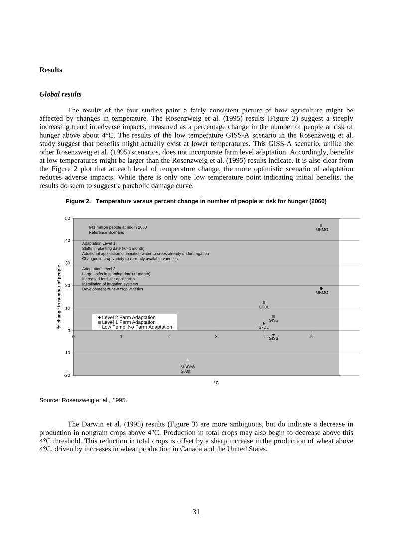
31
Results
Global results
The results of the four studies paint a fairly consistent picture of how agriculture might be affected by changes in temperature. The Rosenzweig et al. (1995) results (Figure 2) suggest a steeply increasing trend in adverse impacts, measured as a percentage change in the number of people at risk of hunger above about 4°C. The results of the low temperature GISS-A scenario in the Rosenzweig et al. study suggest that benefits might actually exist at lower temperatures. This GISS-A scenario, unlike the other Rosenzweig et al. (1995) scenarios, does not incorporate farm level adaptation. Accordingly, benefits at low temperatures might be larger than the Rosenzweig et al. (1995) results indicate. It is also clear from the Figure 2 plot that at each level of temperature change, the more optimistic scenario of adaptation reduces adverse impacts. While there is only one low temperature point indicating initial benefits, the results do seem to suggest a parabolic damage curve.
Figure 2. Temperature versus percent change in number of people at risk for hunger (2060)
-20
-10
0
10
20
30
40
50
0 1 2 3 4 5
°C
% c
han
ge
in n
um
ber
of
peo
ple
Level 2 Farm AdaptationLevel 1 Farm AdaptationLow Temp. No Farm Adaptation
GISS
GFDL
UKMO641 million people at risk in 2060 Reference Scenario
GFDL
GISS
UKMO
Adaptation Level 1:Shifts in planting date (+/- 1 month)Additional application of irrigation water to crops already under irrigationChanges in crop variety to currently available varieties
Adaptation Level 2:Large shifts in planting date (>1month)Increased fertilizer applicationInstallation of irrigation systemsDevelopment of new crop varieties
GISS-A2030
Source: Rosenzweig et al., 1995.
The Darwin et al. (1995) results (Figure 3) are more ambiguous, but do indicate a decrease in production in nongrain crops above 4°C. Production in total crops may also begin to decrease above this 4°C threshold. This reduction in total crops is offset by a sharp increase in the production of wheat above 4°C, driven by increases in wheat production in Canada and the United States.
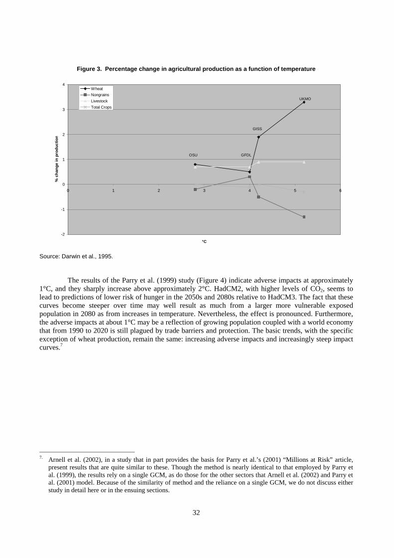
32
Figure 3. Percentage change in agricultural production as a function of temperature
-2
-1
0
1
2
3
4
0 1 2 3 4 5 6
°C
% c
han
ge
in p
rod
uct
ion
Wheat
Nongrains
Livestock
Total Crops
OSU GFDL
GISS
UKMO
Source: Darwin et al., 1995.
The results of the Parry et al. (1999) study (Figure 4) indicate adverse impacts at approximately 1°C, and they sharply increase above approximately 2°C. HadCM2, with higher levels of CO2, seems to lead to predictions of lower risk of hunger in the 2050s and 2080s relative to HadCM3. The fact that these curves become steeper over time may well result as much from a larger more vulnerable exposed population in 2080 as from increases in temperature. Nevertheless, the effect is pronounced. Furthermore, the adverse impacts at about 1°C may be a reflection of growing population coupled with a world economy that from 1990 to 2020 is still plagued by trade barriers and protection. The basic trends, with the specific exception of wheat production, remain the same: increasing adverse impacts and increasingly steep impact curves.7
7. Arnell et al. (2002), in a study that in part provides the basis for Parry et al.’s (2001) “Millions at Risk” article,
present results that are quite similar to these. Though the method is nearly identical to that employed by Parry et al. (1999), the results rely on a single GCM, as do those for the other sectors that Arnell et al. (2002) and Parry et al. (2001) model. Because of the similarity of method and the reliance on a single GCM, we do not discuss either study in detail here or in the ensuing sections.

33
Figure 4. Percentage change in number of people at risk of hunger as a function of temperature
0
10
20
30
40
50
60
0 0.5 1 1.5 2 2.5 3
°C
Per
cen
t ch
ang
e in
num
ber
of
peo
ple
at r
isk
HadCM2
HadCM3
2020s443 ppmv CO2
2020s441 ppmv CO2
2050s527 ppmv CO2
2050s565 ppmv CO2
2080s642 ppmv CO2
2080s731 ppmv CO2
250 million people at risk of hunger in reference scenario.
Source: Parry et al., 1999
Fischer et al. (2002) do not present results as a function of global mean temperature. However, by examining temporal results across various scenarios and knowing how temperature changes for the various GCMs and forcing scenarios, we are able to deduce such results. Figure 5 shows the increase in the number of people at risk of hunger as a function of global mean temperature. Results are shown for two GCMs.

34
Figure 5. Increase in number of people at risk of hunger due to climate change in the 2080s
0
20
40
60
80
100
120
140
160
180
0 1 2 3 4 5 6
Temperature (C)
Mill
ion
s of
Peo
ple
CSIRO
HadCM3
It should be noted that because presenting results in this fashion relies on looking across scenarios, neither CO2 or precipitation is constant. This may help to explain the downturn in number of people at risk in the HadCM3 results. In general, however, both models show that as GMT increases beyond 3°C, the number of people at risk of hunger increases steadily. We are unable to determine how temperature and risk are correlated below 3°C.
Regional results
The regional results presented by Rosenzweig et al. (1995) paint a more complex picture than do the global results alone. Existing disparities in crop production between developed and developing countries were estimated to increase. Under virtually all scenarios of adaptation and climate change, the developing world experiences decreases in production of cereal crops, while the developed world experiences increases. Developing regions average 9 to 11% reductions in production. In contrast, production in developed countries was estimated to increase in all but the UKMO scenario (+11 to -3%). These disparities, coupled with ensuing price increases, translate to increases in the number of people at risk of hunger, most of whom presumably are located in the developing world.
Darwin et al. (1995) also estimated pronounced variations in regional impacts. In Canada, for instance, the only unambiguously high latitude region, not only does production of wheat increase but so does that of other grains, nongrains, livestock, and forest products. In southeast Asia, the model’s only unambiguously tropical region, production of all these commodities, with the exception of nongrains,

35
decreases. These results are a reflection of longer and warmer growing seasons at high latitudes and shorter and drier growing seasons in the tropics. Impacts in midlatitude regions are mixed.
The global results presented by Parry et al. (1999) mask some important regional differences in impacts. For instance, under HadCM2 scenarios, yield increases in high and high midlatitude zones lead to production increases in these regions. Europe and Canada are clear examples of this trend. However, under HadCM3, higher latitudes are predicted to be warmer and drier, and consequently production decreases. Production decreases in lower latitudes under both HadCM2 and HadCM3, part of the reason why negative changes of -3.5 to -16.5% were observed in developing countries. Especially sharp decreases under HadCM2 simulations suggest that the developing world may have a difficult time meeting the challenges of not only a warmer world but also the more variable one that the HadCM2 ensemble simulates. Consequently, the number of people at risk of hunger in the developing regions is estimated to increase, particularly in Africa.
The regional results presented in Fischer et al. (2002) emphasise three general findings. The first is that when aggregated to the global level, impacts are at most a few percent of global agricultural production. Changes in the global GDP of agriculture ranged from –1.5% (HadCM3, A1F1) to +2.6% (DOE-PCM, A2). The second finding is that agriculture in developed counties as a group will most likely benefit from climate change. This does not of course suggest that no developed countries stand to lose. Among developed regions, North America gains substantially in all simulated scenarios. Increases in cereal production of 6-9% are indicated. The Former Soviet Union also mostly benefits from climate induced changes in production. Western Europe proves to be a notable exception to this second finding, where the total extent of potentially good agricultural land systematically decreases, as does the value added by agriculture. The extent of good agricultural land decreases in Northern Europe by 1.5% to 9.6%, particularly in the United Kingdom and Ireland, and by 0.7% to 1.7% in Southern Europe, especially Spain and in Eastern Europe by 0.2% to 5.9%. Decreases were also recorded for East Asia and Japan of 0.9% to 2.5%. Individual countries with decreasing potentially good agricultural land not reflected in regional totals include New Zealand and Venezuela. The third general finding is that most developing regions, with the exception of Latin America, are likely to be confronted with negative impacts. Africa in particular is estimated to experience losses of 2% to 9% in aggregated GDP of agriculture. Northern African, particularly Algeria, Morocco, and Tunisia, as well as Southern Africa and most notably South Africa, experience losses in the extent of potentially good agricultural land, as do Sudan, Mozambique, and Uganda. Significant negative changes in cereal production occur in Asian developing countries, where production declines range from 4% to 10%.
It is clear then that there is tremendous variation in regional results for agriculture, as will be the case in the other sectors that we examine. While it is possible to make generalizations about the nature of regional results, there are always exceptions. While certain regions or countries may experience net benefits or damages on average, a higher resolution analysis suggests that there can be great variation in both the sign and magnitude of impacts on subregional or subnational levels. Although we do not belabour this point in the regional results discussions of subsequent sectors, we do reinforce it in Box 1 by briefly examining agricultural results for one nation.
36
Box 1. A Snapshot of Regional Scale Results: Agriculture in Tanzania
Agriculture is the most important sector of Tanzania’s economy. It comprised 45.1% of GDP in 2000 (World Bank, 2002). Upwards of 80% of the population of the country relies directly on agriculture of one sort or another for a livelihood (Mwandosya et al., 1998). Agricultural production is sensitive to climate change, and country-level impacts could be quite different from change in average global production. Even within the country, there is likely to be substantial regional variation in impacts. A study conducted by the Centre for Energy, Environment, Science and Technology (CEEST) in Dar es Salaam evaluated the risks to agriculture from climate change (Mwandosya et al., 1998). This study relied on the UK89 model (Mitchell et al., 1989) for estimating future temperature and rainfall under a 2xCO2 scenario, where equilibrium was assumed to occur near 2075. The results indicate an increase of 2.5°C to 4°C throughout the country during both winter and summer periods. The pattern of results for rainfall is more complicated, with some parts of the country experiencing increases at times of the year and other parts decreases at certain times. Estimates of the effect of climate change on maize yields in Tanzania are available from model runs of the Crop Environment Resource Synthesis model (CERES-Maize) (Jones and Kiniry, 1986) used by CEEST. The study found that impacts of climate change on three of the country’s most important crops, maize, coffee, and cotton, are likely to be quite different. Furthermore, the estimated yields for any given crop could be different depending on the particular location in question within the country. In general, simulation results show lower maize yields, a result of higher temperatures and, in some cases, decreased rainfall. The average yield decrease over the entire country was 33%, but the simulations produced decreases as high as 84% in the central regions of Dodoma and Tabora. Yields in the northeastern highlands decreased by 22% and in the Lake Victoria region by 17%. The southern highland areas of Mbeya and Songea were estimated to have decreases of 10-15%. Coffee is particularly sensitive to rainfall, both the amount and the number of days of precipitation. Accordingly, coffee production was assumed to depend entirely on rainfall in the CEEST study, which is not unreasonable given that most of the temperatures projected the UK89 model fell well within optimal levels for coffee production. In Lyamunugu, for instance, which is an area of bimodal rainfall where precipitation is predicted to increase, yields are projected to increase by 18%. For Mbozi, located in a unimodal area where precipitation increases, yields are projected to increase by 16%. In general, coffee yields are predicted to increase throughout Tanzania. CEEST’s analysis of the potential impacts of climate change on cotton production in Tanzania parallels that for coffee. Cotton is particularly sensitive to cold temperatures, and is less sensitive to high average temperatures provided water supply is adequate. Temperature changes are not expected to affect yields significantly, because average temperatures would still be within the optimal range for cotton growth. Cotton prefers moderate rain to excessive moisture, and the increases in precipitation projected over much of the country are not expected to be excessive. Consequently, cotton yields would be expected to increase in those locales where precipitation would increase, but would decrease in areas where precipitation is likely to decrease. In general, UK89 projections suggest rainfall might decrease over southern and central parts of the country and increase over the northern parts, where much of the country’s cotton is grown. It is possible then, that any cotton production that is compromised because of climate change could simply shift to the north. Overall, production is likely to increase. Tanzania provides an example of how the picture of regional results can be quite complex and different from that of global results. Depending on the crop in question, regional results might mirror global ones, as with maize, or could well contradict global results, as with coffee and cotton.

37
Other factors
Several final thoughts must be kept in mind with respect to the four agricultural studies we examined. First, while the results we present are generally similar, important realities of food production are not simulated by any of these studies. Agricultural production and even more so risk of hunger can be driven as much by political and social forces as by economic or biophysical forces. Famines typically do not happen only because of climate conditions such as drought but often owe their existence to political factors such as war or the deliberate withholding of food from affected populations. These sorts of factors are virtually impossible to simulate. Second, the studies we examined point to the need for more comprehensive systems of models that simulate the land use dynamics of Darwin et al. (1995), but coupled with the sort of world food supply model used by Rosenzweig et al. (1995) and Parry et al. (1999). The Fischer et al. (2002) study is notable for taking such an approach. However, there are important processes and phenomena that it too neglects. Ideally, the impacts of climate change on other sectors such as water and sea level rise should be included as feedbacks to models of agricultural impacts. Finally, at this point, no successful effort has been made to account for the effects of extreme events on agriculture and how climate change might impact such events and consequently modulate impacts.
Main findings
On the whole it is uncertain whether global agriculture experiences benefits, adverse impacts, or virtually no effect for increases in GMT up to approximately 3° to 4°C. The four studies, however, show that beyond this level there are increasing adverse global impacts. These observations are consistent with the broader literature on agriculture, which shows crop yields declining beyond a global mean temperature increase of approximately 3°C. This phenomenon reflects the knowledge that grain crops, which represent the vast majority of crop revenues, have temperature thresholds beyond which yields decline. This inevitable decline in yields leads to a commensurate decline in outputs. Farmers can grow crops at higher latitudes and altitudes to maintain production within optimal temperature ranges, but eventually this geographical shifting cannot compensate for higher temperatures. What the four studies show and what is consistent with knowledge about crops is the inevitability of eventual declines in production. What is uncertain is where the threshold lies. The studies suggest it lies no higher than 3 to 4°C. However, if climate change results in increased climate variance, greater threat of pests, or less efficient or effective adaptation, the threshold could be lower. Conversely, it is possible that future research and development will result in crops with even higher temperature thresholds.

38
3. SEA LEVEL RISE
We examined three studies that investigated the effects of rising sea level: Fankhauser (1995), Nicholls et al. (1999), and Darwin and Tol (2002b). We present results from the first two of these studies. The third study, Darwin and Tol, demonstrates the sensitivity of the results of the former two studies to choice of metric and assumptions about the value of coastal land and highlights important methodological issues. Nicholls et al. is part of the Special Issue of Global Environmental Change.
Choice of metric
Nicholls et al. focused on the effects of sea level rise on people directly affected and adopted number of people at risk of coastal flooding as their measure. Fankhauser produced estimates of direct cost in dollar terms. The direct cost method includes the cost of dryland and wetland loss, the costs of protection, and the loss of fixed capital. However, while direct cost goes further than estimates of number of people at risk in detailing possible losses, it fails to capture several potentially important effects. It does not take into account the fact that higher prices would be generated by the relatively large losses of land and capital resources from sea level rise. Intuitively, fewer goods and services would be available, and each dollar would buy less. Furthermore, sea level rise is apt to impose costs on land-locked areas as well, via higher prices, and thus reducing welfare. In fact, it is likely there could be spillovers due to international trade. Darwin and Tol developed a method for capturing these sorts of losses with a measure of equivalent variation.
Scenarios
Fankhauser presented the direct costs associated with an assumed 1 m sea level rise by 2100. The Nicholls et al. study used sea level rises of approximately 12 cm, 24 cm, and 40 cm for the 2020s, 2050s, and 2080s, respectively. Darwin and Tol assumed a 0.5 m sea level rise by 2100. As neither Fankhauser nor Darwin and Tol used GCM input, they assumed that sea level rise occurs linearly.
Nicholls et al. developed a flood model algorithm similar to that employed by Hoozemans et al. (1993). This algorithm uses transient output from the HadCM2 (ensemble mean) and HadCM3 GCMs (growth in CO2 concentrations from 354 ppmv in 1990 to 731 ppmv in 2080 for HadCM2 and to 642 ppmv in 2080 for HadCM3) along with results from an ice melt model to derive global sea level rise scenarios. Storm surge flood curves are then raised by relative sea level rise scenarios.
Nicholls et al. did not assume linear rise exogenously, but rather relied on the HadCM2 and HadCM3 outputs, both of which suggest a fairly linear change in sea level. This is an important consideration, since the ability to protect coasts or, even more likely, the speed at which wetlands can migrate inland might be exceeded by sea level rise. More consideration needs to be given to this factor.

39
The Fankhauser and Darwin and Tol studies assumed that adverse impacts associated with sea level derive from the slow but steady loss of wetlands and drylands, and from the protection costs associated with avoiding some of these losses. They did not, however, account for extreme events, an important cause of damage that forms the basis of the Nicholls et al. study. However, the Nicholls et al. study did not consider a change in the level or frequency of storminess, because no such scenarios are available. Instead, Nicholls et al. imposed current levels of storminess on top of expected sea level rise. Nicholls et al. also assumed a 15 cm per century rate of subsidence in those coastal areas that are known to be so affected.
None of the studies considered catastrophic events that might impact sea level suddenly, such as the collapse of the West Antarctic ice sheet. To be sure, such an event would take centuries to be fully realised.
Models
A key difference in how sea level rise adverse impacts are estimated has to do with what is assumed in terms of adaptation. With sea level rise, adaptation typically refers to the decision of whether or not to protect coastal development. Fankhauser and Darwin and Tol assumed an economic paradigm of optimal protection, based on benefit-cost analysis, while Nicholls et al. used a more arbitrary approach based on observed practices. The Fankhauser study minimised the discounted sum of three streams of costs — protection costs, dryland loss, and wetland loss — for each region it considers. Costs are minimised with respect to the percentage of coasts protected. Central to this effort, Fankhauser also developed an expression for determining the optimal degree of coastal protection, where protection efforts are undertaken if the benefits from avoided damage exceed the incremental costs of additional action. One advantage of Fankhauser’s approach is that this trade-off is modelled explicitly, whereas many studies assume exogenously given assumptions about levels of protection. What is not clear is whether this models actual behaviour.
Nicholls et al. estimated land areas threatened by different probability floods arising from the scenarios. These land areas were then converted to people in the hazard zone (the number of people living below the 1000-year storm surge elevation). Lastly, the standard of protection was used to calculate average annual people flooded (the average annual number of people who experience flooding by storm surge) and people to respond (the average annual number of people who experience flooding by storm surge more than once per year).
Finally, Darwin and Tol illustrated the limitations of the direct cost method by using a combined, 12 region, land-use geographic information system and global computable general equilibrium model that estimates both direct costs and equivalent variation, the latter to account for second order economic effects.
Key factors and assumptions
The three studies we examined incorporated different assumptions regarding how sea level rise produces adverse impacts, the underlying socioeconomic baselines, and the nature of adaptation, particularly coastal protection.
Fankhauser and Darwin and Tol produced damage estimates that do not depend in a direct way on population, but simply on the value of land lost from sea level rise and protection costs. Fankhauser assumed that these values are constant, while Darwin and Tol assumed that land values increase with population and economic growth. The Nicholls et al. study depended critically on the evolving population and its distribution. Globally, the study used the same population growth scenario as the other Special

40
Issue studies did (see Table 5). Estimates of the average coastal population density in each nation in the base year were borrowed from Hoozemans et al. (1993). It is assumed that the coastal population is distributed uniformly across the coastal zone. Nicholls et al. projected that population densities increase at twice the rate of national growth.
The studies did not examine all of the consequences of sea level rise. They did not examine changes in salt water intrusion of aquifers or estuaries, nor did they account for the combined effects of sea level rise with potentially increased freshwater runoff via enhanced flooding. They also did not consider the effects of potential changes in coastal storms.
None of the studies captured all possible autonomous adaptations or adaptations that can increase risk (maladaptations), which for sea level rise could be significant. For instance, migration away from the coastal zone, which would be a likely response in frequently flooded areas, was not modelled explicitly, though people to respond may give some indication of this. Each study, however, built in coastal protection as an adaptive response. Darwin and Tol borrowed their approach from Fankhauser, who developed a simple model of optimal coastal protection predicated on a protect or retreat dichotomy. Nicholls et al. examined two scenarios, one with constant protection (1990) and another with evolving standards of protection, which are assumed to be in phase with increasing GNP per capita, though not deliberately responding to sea level rise. This essentially allows for adaptive capacity to be enhanced at higher income levels. The greater costs of protecting deltaic areas relative to other coastal zones were also incorporated into this basic framework.
Spatial scales and distributional issues
While Fankhauser’s model is general and could be applied in a more geographically broad manner, he provided simulation results only for the OECD countries. Nicholls et al., on the other hand, presented regionally and globally aggregated values for results that are calculated on a national level. Darwin and Tol’s analysis is based on a regional level. We are interested primarily in global results, but do highlight regional results where warranted. To a certain extent some adverse impacts from sea level rise are distributed via links of international trade and changes in the prices of goods and services. Only Darwin and Tol used a method that captured these effects, however. Finally, since none of the studies we examined derived benefits associated with sea level rise, globally aggregated results do not run the risk of obscuring regional results that differ in sign.
Results
Global results
The results from both Fankhauser (Figure 6) and Nicholls et al. (Figures 7-9) suggest that adverse impacts increase linearly with sea level rise. As Fankhauser pointed out, one might expect protection costs to rise nonlinearly with sea level rise, based on the fact that construction costs of sea walls increase with required height in such a fashion. This might well be the case, but costs of land loss, overwhelmingly wetland loss, dominate Fankhauser’s bottom line. Ultimately, were wetland loss the only damage associated with sea level rise, this might suggest a levelling off of adverse impacts, since there is a finite area of wetlands to be lost. Fankhauser’s results are sensitive to choice of discount rate and he assumes a discount rate of rate of zero. One important distributional result, which is not depicted in Figure 6, is that poorer nations protect their coasts to a lesser degree. This result has to do not with lack of funds or institutional failure, but because more protection is not cost-effective.

41
Figure 6. Costs of sea level rise in OECD countries
0
500
1000
1500
2000
20
Sea level rise by 2100 (cm)
Bill
ion
s $
100
Source: Fankhauser, 1995
Figure 7. Additional people in the hazard zone as a function of sea level rise
0
10
20
30
40
50
60
70
0 5 10 15 20 25 30 35 40 45
Sea level rise (cm)
Ad
diti
on
al p
eopl
e (m
illio
ns)
HadCM2
HadCM3
2020s
2050s
2080s
Source: Nicholls et al., 1999

42
Figure 8. Additional average annual people flooded as a function of sea level rise
0
10
20
30
40
50
60
70
80
90
0 5 10 15 20 25 30 35 40 45
Sea level rise (cm)
Ad
diti
on
al p
eop
le (
mill
ions
)
HadCM2
HadCM3
2020s
2050s
2080s
Source: Nicholls et al., 1999
Figure 9. Additional people to respond due to sea level rise as a function of temperature
0
10
20
30
40
50
60
70
80
0 0.5 1 1.5 2 2.5 3 3.5
°C
Ad
diti
on
al p
eop
le (
mill
ions
)
HadCM2
HadCM3
2020s
2050s
2080s
Source: Nicholls et al., 1999
Nicholls et al. projected that the number of additional people in the hazard zone also increases linearly as a function of sea level rise. The results displayed in Figures 7-9 assume protection standards

43
evolve as incomes rise, though not in response to sea level rise. The second two curves, which display the results for additional average annual people flooded and people to respond as a function of sea level, exhibit a somewhat steeper increase after a 0.25 m sea level rise, which is assumed to occur by the 2050s. In both cases Nicholls et al. indicated that this is due mainly to the increased frequency of flooding within the existing flood plain as sea level rises. The expansion of the size of the flood plain is a smaller effect.
The Darwin and Tol results are essentially a sensitivity analysis, pointing to the dependence of impacts on assumed land endowments and choice of welfare measure. Current estimates of land endowment uncertainty led to a 36% difference in the results obtained for global direct costs. By using equivalent variation as the welfare measure instead of direct cost, damages are 13% higher on a global level. Regionally, however, equivalent variation can suggest damages of up to 10% lower than direct cost.
Regional results
Nicholls found that most of the people flooded in the 2080s are concentrated in the South Mediterranean, West Africa, East Africa, South Asia, and Southeast Asia. These five regions contain some 90% of the average annual number of people flooded. By way of contrast, in 1990, these regions contained 70% of the average annual number of people flooded. The largest populations at risk are located in South Asia and Southeast Asia, with its densely populated, low-lying deltaic areas. Africa is also at particular risk because of its rapidly growing coastal population and lack of means to achieve high standards of coastal protection. Large relative increases in number of people flooded occur in the small islands of the Caribbean, Indian, and Pacific oceans. By the 2080s, the average annual number of people flooded increases more than 200 times over the reference scenario.
Main findings
In general, we are highly confident that adverse impacts will increase with sea level rise. The studies we examined are consistent with this conclusion; more land will be inundated as sea level rises, damages from higher storm surges will mount, and costs will increase as coastal defences are raised or lengthened to provide necessary additional protection. In addition, there will be other adverse impacts such as increased saltwater inclusion. However, it is impossible to determine whether the relationship between impacts and sea level is a straight line or concave.
These results point to the potential magnitude of simplifying assumptions that studies of global sea level rise make. There is a clear need for methods that do a better job of combining the sorts of costs that each of these studies includes as well as other sources of damage. The value of land, for instance, is an imperfect indicator of the true welfare losses to consumers. Nonmarket values ideally should be incorporated in a more explicit way. Furthermore, responses such as migration out of the coastal zone might mitigate some adverse impacts while introducing a whole new set of costs. Simplifying assumptions about the characteristics of coastal flood plains need revisiting. The importance of extreme events as a driver of adverse impacts induced by sea level rise should be given more attention, and methods must be developed for exploring the potential impact of increased storminess as well as regional changes in storminess. This impact mode could prove to be at least as significant as those that we consider.
It should also be noted that sea levels are expected to continue rising for centuries following any stabilisation of global mean temperatures. For example, Church et al. (2001) show that sea level would continue to rise in response to thermal expansion for two to three millennia beyond the time atmospheric CO2 concentrations are stabilised at a doubling or quadrupling above preindustrial CO2 levels. Sea level would eventually rise 0.5 to 2 m for a doubling of CO2 and 1 to 4 m for a quadrupling. This estimate does not account for additional contributions from ice melt. Thus adverse impacts over time are likely to

44
continue growing. Whether the present value of total damages increases as longer time frames are considered will be substantially influenced by choice of a discount rate.

45
4. WATER RESOURCES
We examined four studies that assessed the potential impacts of climate change on water resources: Arnell (1999), which was part of the Special Issue, Vörösmarty et al. (2000), Alcamo et al. (1997), and Döll (2002).
Choice of metric
The Arnell and Vörösmarty et al. studies focused on assessing the impacts of water stress in general and accordingly relied on measures of number of people at risk. Alcamo et al. (1997) focuses on investigating future scenarios of water scarcity, where climate change is seen as a component of this future, but not the driving factor. It too presents results in terms of number of people affected by water scarcity, among several other metrics. However, Alcamo et al. (1997) presents the results of climate change on water scarcity for only one point in time. Döll focused on agricultural water requirements, and so employed net irrigation requirements as a metric.
Arnell (1999) produced estimates of the number of people living in countries experiencing water stress, as well as estimates of the number of people who live in countries where stress increases less those who live in countries where stress decreases. In this case, a country in a state of water stress is one that is using more than 20% of its available water resources. Vörösmarty et al. adopted a definition and numerical scale of water stress from the United Nations (1997), where stress is defined as the ratio of the demand for water, both agricultural and domestic, to the sustainable water supply to which local populations have access. Vörösmarty et al. defined high water stress as the use of 40% or more of resources.
Alcamo et al. (1997) measure the scarcity of water by means of a criticality index, which combines the criticality ratio (ratio of water use to water availability) and water availability per capita in a single indicator of water vulnerability. The reasoning behind this is that vulnerability increases as two conditions become more critical: (i) total water resources are used up (the critical ratio becomes larger), and (ii) the pressure on existing resources increases (water availability per capita declines). Consequently, under this measure, water scarce regions tend to occur not only in arid regions but also in densely populated areas. The criticality index ranges from 1 for water surplus to 4 for scarcity. The chief difficulty with using the sorts of metrics that Arnell, Vörösmarty et al., and Alcamo et al. (1997) do is the arbitrariness of defining the damage classes (stress versus no stress). There may, for instance, be many people who live just below the stress threshold who are not captured by such a measure. They may suffer adverse impacts that are nearly indistinguishable from those who live in an area that is defined as stressed. In addition, water stress is more likely to be a continuous function than a discrete one. As water supplies become tighter, more and more uses are curtailed and adverse impacts increase.
Scenarios
Arnell used scenarios based on the same HadCM2 and HadCM3 climate change experiments as the other studies that are part of the Special Issue.

46
Arnell followed the convention of the other studies that are part of the Special Issue and presents results for the 2020s, 2050s, and 2080s. The global temperature and precipitation changes associated with these decades for the HadCM2 and HadCM3 model are given in Table 4. The Vörösmarty et al. study adopted a much shorter period of analysis, estimating water stress in only 2025. Both the HadCM2 and CGCM1 models predict changes of not much greater than 1°C at 2025. Alcamo et al. investigate three scenarios of water use (low, medium, and high) and two scenarios of water availability (two different GCMs, see below). Results are presented for two time slices, 2025 and 2075, the latter representing a doubling of CO2 from the reference year, 1995. However the effects of climate change are only presented for 2075. Döll presented results for the 2020s and the 2070s, but not associated temperature changes.
Models
Arnell used a macro-scale hydrological model to simulate river flows across the globe, and then calculated changes in national water resource availability. These changes were then used with projections of future national water resource use to estimate the global effects of climate change on water stress. Vörösmarty et al. used a water balance model that is forced offline with output from the HadCM2 and CGCM1 global climate models. Alcamo et al. (1997) use a global water model, WaterGAP, that computes water use and availability in each of 1,162 watersheds. Some aspects of the models design and data come from the IMAGE integrated model of global environmental change (Alcamo et al., 1994). WaterGAP takes into account socio-economic factors that lead to domestic, industrial and agricultural water use as well as physical factors that determine supply (runoff and ground water recharge). The study relies on two GCMs for physical and climatic input, ECHAM4-OPYC and GFDL. Döll used a global model of irrigation requirements (GIM), which is based on a global map of irrigated areas that shows the fraction of each cell that was equipped for irrigation in 1995. Net irrigation was computed as a function of climate and crop type, with climatic input generated by two transient climate models, the ECHAM4/OPYC3 model and the HadCM3 model, both with IS92a type forcing.
Key factors and assumptions
Each of the studies we examined made a number of important assumptions that must be outlined before we consider their results. As with agriculture, these assumptions can be divided into three classes: those related to biophysical processes, baseline socioeconomic scenarios, and those related to adaptation. One biophysical assumption, which is shared by both Arnell and Vörösmarty et al., is that change in runoff is regarded as change in water supply. This is essentially true for Alcamo et al. (1997) as well, though they include groundwater recharge as part of water supply. However, in practice, not all of this runoff may be available for use, and the proportion that will be available varies significantly across countries. This may have much to do with how concentrated flows are in time and the infrastructure employed to capture and store water for later use. Furthermore, water use is equated with withdrawals from surface water or groundwater in all these studies. Accounting for water use on a purely consumptive basis in this manner may overstate water use. This approach does not account for return flow, for instance, or instream use. The Arnell study further assumes that people within a nation have equal access to the water resources of that nation. Another point is that none of the studies incorporated the effect of increased CO2 or climate change explicitly on projections of water use. This is a particularly important limitation of the Döll study, since it focused on irrigation requirements. For example, inclusion of the CO2 fertilisation in the U.S. National Assessment led to a conclusion that demand for irrigation would decrease (NAST, 2000). Agricultural use is an important component of future projections of total use, so this is an important omission even in the Arnell and Vörösmarty et al. studies. Also, none of the studies examined the impacts of flooding or changes in interannual and interseasonal variance in general. Since an increased hydrologic cycle is likely

47
to accompany climate change (Houghton et al., 2001), increased risk of flooding in many parts of the world is also likely.
Baseline assumptions in these studies are critical. Population is an important component of the water use picture as well since the exposure assessment in both Arnell and Vörösmarty et al. Arnell used the population projections shared by the other studies that make up the Special Issue (Table 5). Alcamo et al. (1997) rely on similar projections that are based on the IPCC’s IS92a scenario. Care must be taken in comparing results from the Alcamo et al. and Vörösmarty et al. studies to the Arnell study because of, among other issues, their assumptions regarding population. Not only did the studies assume different cumulative global populations, but the initial distribution of this population between the various classes of water stress differs as well. Arnell, Vörösmarty et al., and Alcamo et al. (1997) assumed that efficiency in agricultural and industrial water use increases. Arnell explored different projections based on different rates of economic growth and technological improvements. Initially, the greatest gains in efficiency are made in western countries. Eventually, however, non-OECD domestic and industrial usage is projected to converge to that of the OECD. The Alcamo et al. (1997) study’s assumptions concerning water use are shown in Table 6. In their projections, industrial water use dominates total usage in developed countries in the future. In general, industrial use is projected to increase as GDP rises.
Table 6. Water use scenarios
Scenario Domestic Industry Agriculture L Water intensity
increases with income up to $15,000/cap-yr then rapidly declines by 50% and then further to a stringent water conservation target value for domestic water use.
Water intensity is constant with income up to either $5,000 or $15,000/cap-yr then rapidly declines by 50% and then further to a stringent water conservation target value for industrial water use.
Irrigated area constant. Water use efficiency improves.
M (best guess) Water intensity increase with income up to $15,000/cap-yr then declines by 50% and remains constant afterwards.
Water intensity is constant with income up to either $5,000 or $15,000/cap-yr then declines by 50% and remains constant afterwards.
New irrigation areas in most developing countries. Water use efficiency improves.
H Water intensity increase with income up to $15,000/cap-yr. Afterwards remains constant.
Water intensity increases with income up to either $5,000 or $15,000/cap-yr. Afterwards remains constant.
New irrigation areas in most developing countries. Water use efficiency does not improve.
Scenario L = low, scenario M = medium, scenario H = high.
The inclusion of adaptation in the studies of water we reviewed is fairly limited. Land use in the water demand projections employed in both Arnell and Vörösmarty et al. was assumed to remain constant. Similarly, Döll assumed that the amount of land under irrigation remains constant. The WaterGAP model
48
used by Alcamo et al. (1997) incorporated land use change. Vörösmarty et al. did allow for migration within countries to sources of water but on a limited scale. Döll made several concessions to adaptation by allowing for changes in the timing of the growing season and cropping patterns.
Spatial scales and distributional issues
Aggregation of results to a global level poses significant problems in studies of the impacts of climate change on water resources. Most problems stem from lack of data and the choices of indices and spatial scales of analysis that available data impose. Assessments of water resources and climate generally examine impacts at the basin level because water resources are typically managed at the basin or sub-basin level (see Arnell, 1999, and Liu, 2001). Arnell, however, examined water resources results at the national level. Not only does this not capture basin to basin variation, but small changes in hydrological conditions can also lead to very large changes in the estimated number of people facing water stress. This is the case if populous countries are near the threshold. Furthermore, these national level indices can hide substantial within-country variation and underestimate the number of individuals living under water stress conditions. Vörösmarty et al. got around this problem by relying on a grid based approach that uses spatially disaggregated data on water use at the water basin level. The lack of spatially disaggregated data was one of the chief hurdles to previous grid based approaches. Vörösmarty et al. detailed a method for disaggregating country level water statistics. Alcamo et al. (1997) calculated water balance on the grid level (0.5º latitude by 0.5º longitude) but aggregated to the watershed and national level. Döll also conducted her analysis at 0.5� by 0.5�grid level and presented regionally aggregated and basin aggregated results. Because, in general, water is not an internationally transferable good in the way that agricultural commodities are, care must be taken in the analysis of global or even regional results, which can obscure important adverse regional impacts.
Results
Since global results are an aggregation of regional results, we discuss them together.
The results from the water studies are far less conclusive than those of other sectors. Figure 10, based on Arnell’s results, indicates the changes in the number of people living in countries experiencing water stress with increasing temperature. There is not much change in water stress by this measure between the 2020s and the 2080s, with the exception of a reduction in the numbers experiencing stress in the 2050s. This reduction is the result of the United States and the United Kingdom moving out of a condition of stress. As might be expected, the relatively wetter HadCM2 model predicts fewer people living in water stressed conditions. Figure 11, which shows the difference between the total population of countries where stress increases and the total population of countries where stress decreases, attempts to give a better sense of the total number of winners versus losers with regard to changes in water stress, regardless of arbitrary thresholds. The trend is still ambiguous, since one model predicts net loss (HadCM2) and another predicts net gain (HadCM3). Counter to what one might expect, it is the drier model (HadCM3) that predicts a larger population of people in countries where water stress decreases. This is driven mainly by the fact that in the HadCM2 scenario, stress increases in the populous countries of India and Pakistan, while in the HadCM3 scenario, stress decreases in these countries. In both figures, the results are sensitive to large countries flipping from one situation to another. Regionally, the countries where climate change has the greatest adverse impact on water resource stress are located around the Mediterranean, in the Middle East, and in southern Africa. Significantly, these countries are generally least able to cope with changing resource pressures. Overall, these results indicate the importance of the regional distribution of precipitation changes to estimates of water resource impacts.
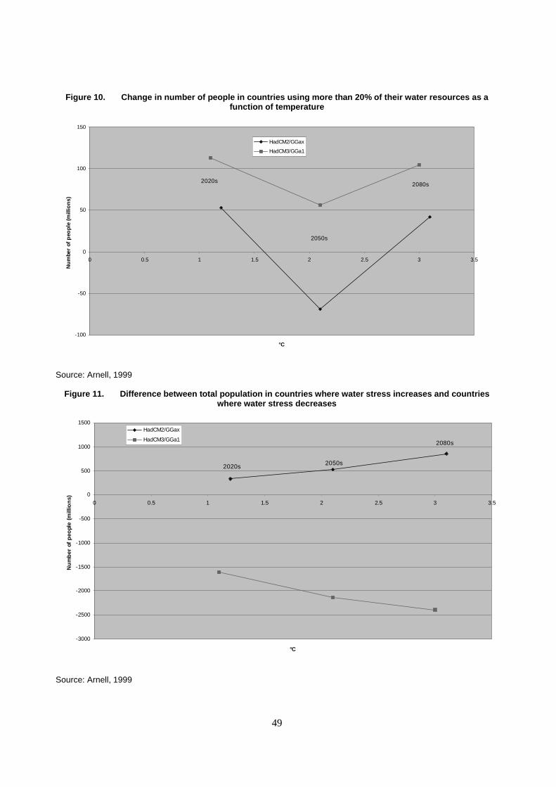
49
Figure 10. Change in number of people in countries using more than 20% of their water resources as a function of temperature
-100
-50
0
50
100
150
0 0.5 1 1.5 2 2.5 3 3.5
°C
Nu
mbe
r of
peo
ple
(mill
ion
s)
HadCM2/GGax
HadCM3/GGa1
2020s
2050s
2080s
Source: Arnell, 1999
Figure 11. Difference between total population in countries where water stress increases and countries where water stress decreases
-3000
-2500
-2000
-1500
-1000
-500
0
500
1000
1500
0 0.5 1 1.5 2 2.5 3 3.5
°C
Nu
mb
er o
f p
eopl
e (m
illio
ns)
HadCM2/GGax
HadCM3/GGa1
2020s 2050s
2080s
Source: Arnell, 1999

50
Vörösmarty et al.’s results indicate that climate change has little effect globally on water resource pressure. The effects of increased water demand due to population and economic growth eclipse changes due to climate. Here again it is important to note regional changes, which are masked by global aggregates. Vörösmarty et al. predicted significant water stress for parts of Africa and South America. This is offset by estimated decreases due to climate change in Europe and North America. In general, climate change produces a mixture of responses, both positive and negative, that are highly specific to individual regions. Of course, there is only a limited amount of climate change by 2025, the date at which the Vörösmarty et al. analysis ends.
Alcamo et al. (1997) present results that highlight the impact of climate change on future water scarcity for only one point in time, 2075, and for one of the two GCMs that the study employed. The study suggests that globally, overall annual runoff increases and water scarcity is somewhat less severe under climate change. In a world without climate change, 74% of the world’s population is projected to live in water scarce watersheds by 2075. However, with climate change, this figure is only 69%. These results are consistent with those of Vörösmarty et al., suggesting that climate change is not the most important driver of future water scarcity. Growth in water use due to growth in population and economies is the decisive factor. Economic growth and concomitant increase in industrial water demand are particularly important. This is illustrated by projections for Africa, which suggest that despite large increases in population, water use (per capita) does not increase accordingly, because income remains low. Though Alcamo et al. (1997) suggest that climate change may ameliorate water scarcity globally, regionally the picture is quite different. Some 25% of the earth’s land area experiences a decrease in runoff in the best guess scenario according to Alcamo et al. (1997), and some of this decrease is estimated to occur in countries that are currently facing severe water scarcity. Decreases are estimated to occur in northern Brazil, Chile, Taiwan and the Indian west coast. Countries such as Cyprus, Israel, Jordan, and Morocco, which already experience severe scarcity, are projected to have even less runoff. The Alcamo et al. (1997) results also point to the possibility that industry will supersede agriculture as the world’s largest user of water.
Döll’s results mirror those of Vörösmarty et al. When cell specific net irrigation requirements are summed over world regions, increases and decreases of cell values caused by climate change average out. Irrigation requirements, however, increase in 11 out of 17 of the world’s regions by the 2020s, but not by more than 10%. By the 2070s, increases occur in 12 of these regions, 10 of which also show an increase in the 2020s. The highest absolute increases were predicted for South Asia, and the highest relative increases were predicted for Southeast Asia, where irrigation requirement per hectare are currently low. Net irrigation requirements in Northern Africa and the Middle East were predicted to decrease, even though temperatures increase and precipitation decreases in the major irrigated parts of these regions. This can be accounted for by a climate change induced shift of the optimal growing seasons from summer months to winter months, when solar radiation and consequently evapotranspiration are lower.
Our analysis of the relationship between water resources and climate change is inconclusive. Averaging world regions or even countries presents many problems. River basins probably represent a better unit of analysis. The study that examined impacts on water availability and use at the basin level considered only a limited magnitude of climate change.
Other factors
Water use in the future, with or without climate change, is a complicated issue that is difficult to simulate. Much of the problems that climate change causes in this sector could be amplified or overwhelmed by challenges related to infrastructure and associated water services. Potentially large economic costs are likely to be associated with responses or with the consequences of inaction. Where water stress is greatest, costs may also include the curtailment of economic activities, the abandonment of

51
infrastructure, migration, and, as some scholars have suggested, the possibility of conflict, Vörösmarty et al. pointed out. These are difficult costs to begin to capture. Furthermore, the challenge in the future may be as much about how to provide clean supplies of water as it might be about providing adequate quantity. Much of these difficulties may be focused in growing large urban areas, which face major problems related to infrastructure, water pollution, and the control of waterborne disease (United Nations, 1997).
In addition, it is difficult to assess water impacts at such a large scale. Water resources are managed at the level of basins, which do not necessarily conform to political boundaries or grid cells. Impacts may differ from one basin to the next.
To develop a more complete analysis of the future impacts of climate change on water resources, it is important to consider a number of factors and systems more thoroughly. These include the climate variance, water engineering, human systems (in particular legal and institutional issues), and adaptation. Also, better socioeconomic data to improve projections of future water use on a spatially disaggregated level will be important.
Main findings
A clear relationship between increasing magnitude of climate change and impacts on water resources does not emerge from this analysis. An argument can made that adverse impacts to the water resources sector will probably increase with higher magnitudes of climate change.8 This argument is based on two considerations. One is that water resource infrastructure and management are optimised for current climate. The further future climate diverges from current conditions, the more likely it is that thresholds related to flood protection or drought tolerance will be exceeded with more frequency and with greater magnitude than they currently are. The second consideration is that more severe floods and droughts are expected to accompany higher magnitudes of climate change. Some regions might benefit from a more hydrologically favourable climate, but it seems unlikely that the majority of the world’s population would see improved conditions, especially since systems are optimised for current climate. It might be possible to retune systems to changed climate, but the cost and difficulty of doing so would probably only increase as the magnitude and rate of climate change increased.
One critical reason why we do not see a clear relationship between increases in GMT and effects on water resources has to do with changes in precipitation. An increase in global mean temperature would increase global mean precipitation. However, the nature of regional changes in precipitation is quite uncertain. Where exactly the additional precipitation falls is not certain. Differences in precipitation patterns from one climate model to another are probably more important than differences in mean temperature in terms of their effect on estimates of how water resources will be impacted.
An additional reason that some of the analyses do not yield a clear trend is the scale at which they were conducted. The water basin is the critical unit for analysis of water resources. Changes in one part of a basin, such as increased or decreased runoff, will affect other parts of the basin. Typically, such changes have little effect outside of the basin (unless one basin feeds into another or is connected to another via
8. Arnell et al. (2002) and Parry et al. (2001) differ in their conclusion concerning water stress. They both present
results that suggest steadily increasing numbers of people at risk of water shortage as global mean temperature increases, both for the 2050s and the 2080s. However, Arnell et al. (2002) consider only the numbers of people already living with water stress who would experience an increase in stress due to climate change. This approach neglects the those people for whom water stress decreases and in general neglects the impacts, negative or positive, on those people who do not currently live in water stressed countries. Essentially, this study considers losers only and provides no sense of net impacts.

52
water transport infrastructure). Since basins do not conform to national borders, an analysis that is based on estimating a uniform change for individual countries may not capture realistic impacts on water resources.
Beyond this, the impacts on water resources are extremely complicated and can depend on such factors as how water is consumed, the ability to adjust uses, legal and institutional constraints, and the capacity to build or modify infrastructure. These and other factors make it difficult to reach a conclusion about the relationship between climate change and water resource impacts.

53
5. HUMAN HEALTH
The effects of climate change on human health could find expression in numerous ways. Some health impacts would doubtless result from changes in extremes of heat and cold or of floods and droughts. Others might result indirectly from the impacts of climate change on ecological or social systems. The former might include a higher incidence of strokes and cardiovascular disease associated with heat stress as well as potential reductions in cold-related health impacts and increases in water-borne disease transmission. Among the latter could be changes in infectious disease occurrence, increased incidence of respiratory disease related to concentrations of local air pollution, changes in rates of malnutrition, and impacts related to large-scale human migration or economic disruption (McMichael et al., 2001).
Assessing the impacts of climate change on human health in any comprehensive way is extraordinarily difficult. Health impacts are complex and owe their causes to multiple factors. They may lead to increases in morbidity and mortality. Vulnerability will differ from one population to another and within every population over time (McMichael et al.). In general, there is insufficient literature to begin to form other than the most rudimentary conclusions concerning overall health impacts. Malaria transmission is the only impact category where several studies with good global and temporal coverage exist. The impacts of climate change on vector borne disease are unlikely to be limited to malaria (dengue and schistosomiasis are likely possibilities), but malaria might be representative of how climate change may affect the risks of vector borne diseases in general. Consequently, we focused on three studies that assessed the possible impacts of climate change on the global transmission of malaria. The studies of malaria we examined are Martin and Lefebvre (1995), Martens et al. (1999), and Tol and Dowlatabadi (2002).
There is a growing indication that waterborne diseases may be an extremely significant source of climate change induced health risk. Climate change is likely to lead to increased water stress and deteriorate water quality in some areas, which in turn might well increase the incidence of water borne diseases. Several studies suggest that there is in fact a correlation between average annual temperature and the incidence of diarrhoeal diseases. However, these studies are limited in the range of temperatures they examine or are not yet published. We present the results of one such study, Hijioka et al. (2002), in abbreviated fashion. We also briefly examined Tol’s (1999 a and b) results of how mortality is influenced directly by changes in temperature, both high and low.
Choice of metric
Both Martens et al. and Martin and Lefebvre characterised the risk of increased malaria transmission. Martens et al. estimated changes in the number of people at risk of malaria infection, while Martin and Lefebvre estimated changes in the area of potential transmission. Tol and Dowlatabadi provided estimates of the increase in mortality, but these estimates are based on those of other studies, which only go so far in estimating malaria potential.

54
Scenarios
Martens et al. relied on the transient scenarios that are shared by the other Special Issue studies (see Table 4 for associated temperature and precipitation anomalies). Martin and Lefebvre assessed the impacts of a doubling of CO2, though they did not state their assumptions about when equilibrium is achieved. They used climatic output from the following set of GCMs: GISS, GFDL, UKMO, and OSU (see Table 3). Tol and Dowlatabadi’s period of analysis ends in 2100. The climate change simulations in Tol and Dowlatabadi are endogenous, based on scenarios of greenhouse gas emissions that are tied to economic activity.
Models
The relationship between climate and human health is complex (Balbus and Wilson, 2000). A number of factors, ranging from the ecology of disease vectors to how access to public health services is determined by level or income or development, must be understood well to make reliable predictions of the effect of climate change on malaria mortality and morbidity.
Martin and Lefebvre used a model of malaria that predicts potential transmission, which occurs when environmental conditions are favourable at the same time and same place to both malaria parasites and malaria vectors. The model also makes prediction based on endemicity, where seasonal transmission occurs when the conditions are favourable for 7 or fewer months of a year; perennial transmission occurs when the favourable conditions exist for 8 months per year or more.
The Martens et al. study is based on a model of malaria that is part of the MIASMA model. This model is more sophisticated than that of Martin and Lefebvre in that it includes estimates regarding the distribution of 18 different malaria vectors, species-specific relationships between temperature and transmission dynamics, and a more realistic approach regarding malaria endemicity (epidemics versus year-round transmission).
Tol and Dowlatabadi relied on the integrated model FUND (Tol, 1997) and developed a simple model of vector borne disease, which is parameterised from the results of studies of malaria potential. They relied on three other studies of climate change and malaria to parameterise their meta-model. An increase in potential is assumed to create an analogous increase in incidence.
Key factors and assumptions
Martin and Lefebvre’s model is the simplest of those we consider. It does not consider the epidemiology of malaria transmission or human interaction of any kind. Predictions of malaria potential are based entirely on the coincidence of the proper climatic conditions in the same location necessary to ensure the theoretical survival of vector and parasite. The model does not account for adaptation, land use change, control efforts, biogeographical change, or extreme events. Nor does it take into account potential barriers to vector migration, physical or ecological.
Martens et al. employed an approach that is somewhat more sophisticated. While it incorporates significant epidemiological insight such as survival of vectors as a function of daily temperature, mosquito species distribution is assumed to be unchanged by climate. Changes in potential transmission are based entirely on climate driven impacts on parasite life cycle, vector survival and longevity, and vector-human interaction. This model also does not allow for land use change or control efforts. Tol and Dowlatabadi transformed the results from several studies predicting risk of malaria transmission to actual mortality.

55
They did this by assuming that the current regional death tolls from malaria increase as the risk of potential transmission increases with temperature.
All three studies attempted to account for baseline socioeconomic changes. Martin and Lefebvre compared their results to a World Health Organization (WHO) map or malaria distribution for 1992. Martens et al. used a gridded data base of population distribution and linked it via a relational database to World Bank midrange projections of population shared by the other Special Issue studies. Future population distributions are estimated for the three time slices that correspond to the analysis, the 2020s, 2050s, and 2080s. Tol and Dowlatabadi’s scenarios of demographic and economic change are based on those of the Energy Modeling Forum’s Standardised Scenario. They assumed that population changes within a region are homogenous.
Neither the Martens et al. study nor the Martin and Lefebvre study incorporated adaptation of any kind. This is a significant limitation because the strength of the public health system is a critical factor determining risk to infectious disease (Patz et al., 2000). Tol and Dowlatabadi explored the importance of access to public health services on malaria mortality by assuming a linear relationship between access to public health services and regional per capita income. They then developed a simple model for relating income, temperature, and vector borne disease mortality. Scenarios of mortality with and without a baseline of economic growth were then considered.
Spatial scales and distributional issues
The estimates of change in population at risk of malaria in Martens et al. are presented by region, though the model is structured on a grid cell scale. It should be noted that the MIASMA model on which this study relied has not been validated at a global level because of the uncertainty regarding the natural limits of malaria distribution, which stems from a lack of historical records describing the presence of malaria, and also the instability of malaria transmission at the fringes of this zone, where only infrequent transmission occurs. It has, however, been validated successfully at country and regional levels. Results presented on a global basis represent the aggregation of regional results. The Malaria Potential Occurrence Zone model that Martin and Lefebvre used operates with grid squares of 0.5° latitude by 0.5° longitude. Results are presented on the grid level cartographically and as global aggregates. The FUND model that Tol and Dowlatabadi used is specified with different geographical resolutions for socioeconomic and physical aspects of their simulations. The atmospheric physics and climate change simulations of FUND are simulated globally. The socioeconomic components are aggregated into nine major world regions.
Results
Global results
The studies tend to portray an increase in health risks with increasing temperature. Martin and Lefebvre (Figure 12) suggested that a global increase of seasonal potential malaria transmission zones is caused by the encroachment of seasonal zones on perennial ones and by the expansion of seasonal malaria into areas formerly free of malaria. The increase in area of potential transmission in all malarious zones seems to be linear and increasing with temperature.

56
Figure 12. Percentage change in extent of potential malaria transmission as a function of temperature
-60
-40
-20
0
20
40
60
0 1 2 3 4 5
°C
Pec
ent
chan
ge (
%)
Seasonal
Perennial
All malarious zones
OSU GFDL GISS UKMO
Source: Martin and Lefebvre, 1995
The results from Martens et al. are shown in Figures 13 and 14. Figure 13 depicts the additional people at risk for falciparum malaria and Figure 14 depicts additional people at risk for vivax malaria, for both the HadCM2 and HadCM3 models. Year-round transmission appears to increase linearly with temperature for both types. However, the risk of epidemics is reduced and in both cases decreases gradually with temperature. It is more difficult to draw conclusions about seasonal transmission, though in the case of falciparum, at least, risk also seems to decrease with rising temperature. In both cases, these measures risk missing potential increases in the actual disease burden. The portion of the year during which transmission can occur might increase, but if the increase is not enough to trigger a change in risk category, as defined in the study, this increase will not register. The results could, however, indicate an expansion of year-round transmission at the expense of seasonal and epidemic transmission, coupled with an expansion at the fringes of malarious zones, mostly likely in the form of epidemic transmission potential.
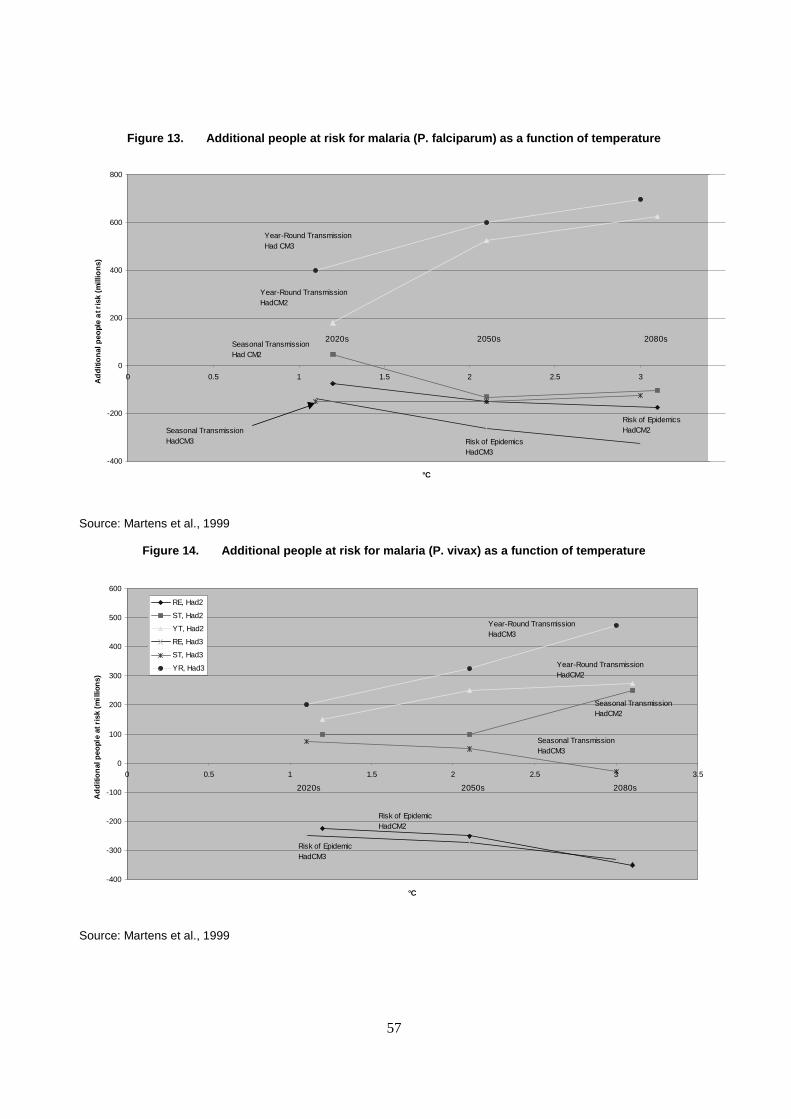
57
Figure 13. Additional people at risk for malaria (P. falciparum) as a function of temperature
-400
-200
0
200
400
600
800
0 0.5 1 1.5 2 2.5 3
°C
Ad
diti
on
al p
eopl
e a
t ris
k (m
illio
ns)
Year-Round TransmissionHad CM3
Year-Round TransmissionHadCM2
Seasonal TransmissionHad CM2
Seasonal TransmissionHadCM3 Risk of Epidemics
HadCM3
Risk of EpidemicsHadCM2
2020s 2050s 2080s
Source: Martens et al., 1999
Figure 14. Additional people at risk for malaria (P. vivax) as a function of temperature
-400
-300
-200
-100
0
100
200
300
400
500
600
0 0.5 1 1.5 2 2.5 3 3.5
°C
Ad
diti
on
al p
eopl
e at
ris
k (m
illio
ns)
RE, Had2
ST, Had2
YT, Had2
RE, Had3
ST, Had3
YR, Had3
Year-Round TransmissionHadCM3
Year-Round TransmissionHadCM2
Seasonal TransmissionHadCM2
Seasonal TransmissionHadCM3
Risk of EpidemicHadCM2
Risk of EpidemicHadCM3
2020s 2050s 2080s
Source: Martens et al., 1999

58
Aggregating these various modes of transmission and types of malaria is not straightforward.9 For instance, an increase in risk of year-round transmission is not necessarily more serious than an increase in risk of seasonal transmission. In fact, the reverse could well be true in many locations. Populations exposed to malaria year-round often develop a higher immunity than do those exposed less frequently. Arguably, one could simply sum the number of people at risk for malaria, regardless of endemicity or variety of parasite. Though this clearly mixes types of risk, it would provide some crude indication of how the total number of people exposed to malaria might change with climate. Doing this in Figure 13 or Figure 14 would yield an increasing trend, suggesting that the number of people at risk of malaria over the next century does increase. This could be the case. However, given that different sorts of malaria risk are likely to have different implications for actual mortality and the pitfalls in interpretation that result from aggregation, we do not do so.
Tol and Dowlatabadi took the approach of converting risk of potential transmission to mortality, which allows for aggregation across different endemicities smoothly. However, Tol and Dowlatabadi provided results of mortality as a function of only time and not temperature. They did, though, show that by the last decade of the century, global mortality from malaria is reduced to virtually zero as a result of economic growth and presumably better access to public health services.
Regional results
Several regional results are worth noting. The number of people at risk of seasonal transmission increases strongly in Africa. This is due primarily, according to Martens et al., to some regions becoming too dry and consequently moving from year-round transmission to seasonal transmission. For example, a similar change occurs in Southern Africa, where risk of seasonal transmission changes to risk of epidemics because of a decrease in precipitation. Additional numbers of people at risk increase most in regions where climate is currently unsuitable for the parasite to thrive, but the vector is nonetheless present. In the Eastern Mediterranean, climate change is predicted to transform current no risk areas into areas of potential transmission risk. Conversely, in Central America, malaria transmission zones are already limited by vector distribution, and consequently, the model does not predict increases in number of people at risk here (vector distribution is assumed to be constant).
Other factors
It is important to point out the inadequacy of both malaria potential as a risk indicator and existing attempts to convert this to risk potential to actual mortality. The biggest problem with the first approach is that it does not account for public health measures to control malaria. For example, much of the United States is a potential malaria transmission zone, but the risks are low because of public health measures (Patz et al., 2000). An additional problem is that in regions that are already saturated with
9. Arnell et al. (2002) and Parry et al. (2001) present results for additional millions of people at risk of malaria, for
both the 2050s and the 2080s, that suggest a steadily increasing trend between temperature increases of 0° and 3°C. These studies rely on a method and socioeconomic assumptions that are quite similar to those of Martens et al. Both studies look at the total additional population living in an area where the potential for malaria transmission exists. The two studies differ from Martens et al. only in how they aggregate results. Results are aggregated across different types of risk, as defined by seasonality of transmission. Total aggregate results include the populations of all areas that experience an increase in potential transmission and where the duration of the transmission season is at least one month per year. Furthermore, results are presented for only one malaria parasite, falciparum, and much of the increase that is indicated is for what is most likely epidemic transmission in developed countries, where public health infrastructure makes it unlikely that such a risk would be realized as a significant disease burden.

59
malaria, an increase in potential would not be likely to result in an increase in incidence. In those regions that are free of malaria, a small increase in potential transmission could have serious effects on incidence. Furthermore, despite the obvious difficulties of converting risk potential to mortality, doing so does not capture morbidity, potentially an even more important cost globally. In addition, humans are capable of developing partial immunity when exposed to malaria infections regularly. Consequently, it is possible that the burden of disease is actually lower in an area with year-round transmission than in an area characterised by seasonal transmission.
Finally, any comprehensive effort to assess the potential impacts of climate change on human health must be much broader in scope than an analysis of one vector borne disease. The potential exists for climate change to affect human health via a number of avenues. Both vectors and the infectious diseases they bear are likely to be affected by changes in temperature and precipitation. In the following section, we touch on the possibility that climate change could influence health directly, by its impact on temperature extremes, both high and low. However, climate change could also affect the proliferation of infectious diseases not borne by vectors. Extreme events such as heat waves or floods are accompanied by the possibility of mortality or morbidity. Finally, human health might be affected indirectly by the effects of climate change on agriculture (malnutrition) or water resources. There is little if any attention devoted to these other avenues in the literature.
Water borne disease
Hijioka et al. (2002) developed a statistical model to explain the current incidence of diarrhoeal disease in 13 world regions. The model relies on two explanatory variables, water supply coverage and annual average temperature. The increase in diarrhoeal incidence, expressed as incidence per capita per year, is approximately 7.3% for a temperature increase of 1°C. This figure is similar to what previous research has estimated (e.g., Checkley et al., 2000) This model is then coupled with a second that estimates future scenarios of water supply coverage as a function of income, to produce an equation for the estimation of diarrhoeal incidence as a function of temperature change. This equation simultaneously accounts for the reduction in water borne diarrhoeal incidence resulting from improvements in the water supply coverage and related sanitary conditions in developing countries (due to increasing income) and for the increase in diarrhoeal incidence resulting from the proliferation of pathogens and promotion of putrefaction due to increased temperatures in both developing countries and developed countries.
Hijioka et al. investigated the results for four scenarios of emissions, temperature change, and socioeconomic development. These are the A1B, A2, B1 and B2 scenarios from the Special Report on Emission Scenarios. They use a simplified climate model to produce global temperature changes based on the emissions associated with each of these scenarios, the results of which are then scaled to the 13 regions based on the future climate spatial distribution generated by the NIES/CCSR GCM (IS92a forcing).10 Future scenarios of water supply coverage are developed based on a second statistical model that relies on economic growth (per capita GDP) as the independent variable. Rates of economic growth are specified in the SRES scenarios.
10. Scaling GCM output based on the IS92a scenario to reflect SRES scenarios does raise a concern, particularly at
the regional scale. The IS92a scenario assumes relatively high emissions of sulfate aerosols, which can have a strong cooling effect. This can result in some regions being much cooler than they are in lower aerosol emissions scenarios. Scaling assumes that the magnitude changes in proportion with global mean temperature. Under the SRES scenarios, we could reasonably expect a projection of higher temperatures in many regions relative to the IS92a scenario.
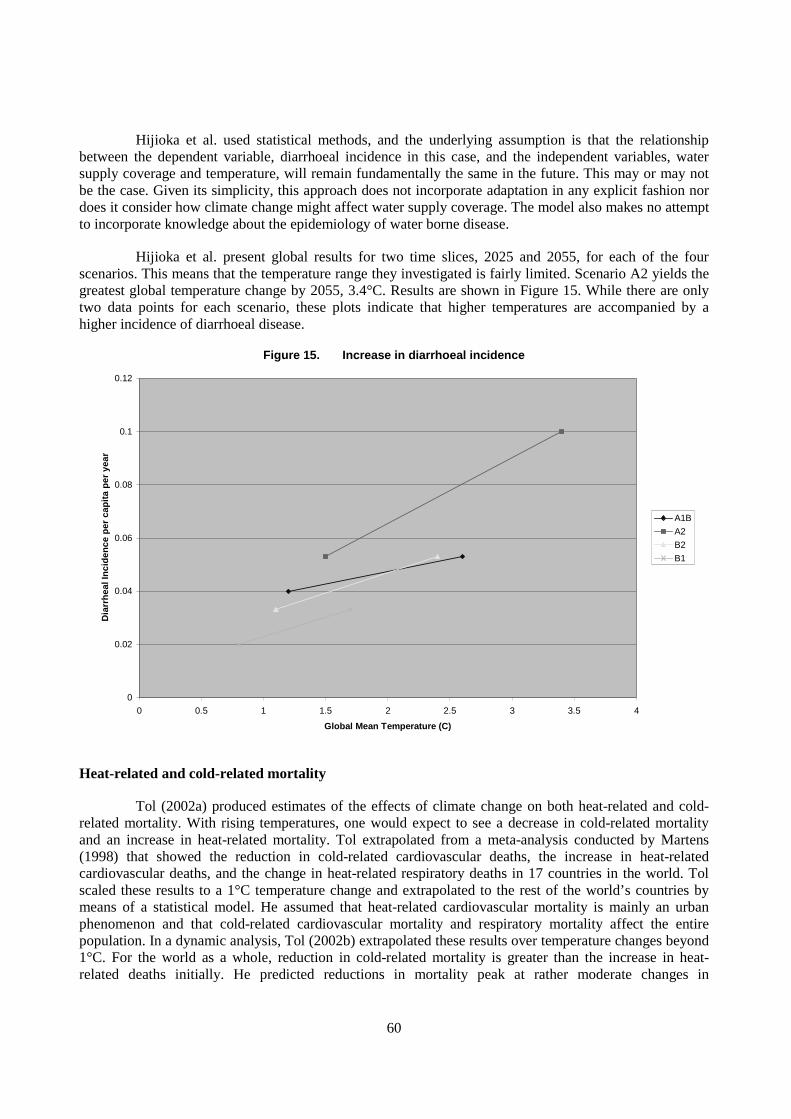
60
Hijioka et al. used statistical methods, and the underlying assumption is that the relationship between the dependent variable, diarrhoeal incidence in this case, and the independent variables, water supply coverage and temperature, will remain fundamentally the same in the future. This may or may not be the case. Given its simplicity, this approach does not incorporate adaptation in any explicit fashion nor does it consider how climate change might affect water supply coverage. The model also makes no attempt to incorporate knowledge about the epidemiology of water borne disease.
Hijioka et al. present global results for two time slices, 2025 and 2055, for each of the four scenarios. This means that the temperature range they investigated is fairly limited. Scenario A2 yields the greatest global temperature change by 2055, 3.4°C. Results are shown in Figure 15. While there are only two data points for each scenario, these plots indicate that higher temperatures are accompanied by a higher incidence of diarrhoeal disease.
Figure 15. Increase in diarrhoeal incidence
0
0.02
0.04
0.06
0.08
0.1
0.12
0 0.5 1 1.5 2 2.5 3 3.5 4
Global Mean Temperature (C)
Dia
rrh
eal I
nci
den
ce p
er c
apit
a p
er y
ear
A1B
A2
B2
B1
Heat-related and cold-related mortality
Tol (2002a) produced estimates of the effects of climate change on both heat-related and cold-related mortality. With rising temperatures, one would expect to see a decrease in cold-related mortality and an increase in heat-related mortality. Tol extrapolated from a meta-analysis conducted by Martens (1998) that showed the reduction in cold-related cardiovascular deaths, the increase in heat-related cardiovascular deaths, and the change in heat-related respiratory deaths in 17 countries in the world. Tol scaled these results to a 1°C temperature change and extrapolated to the rest of the world’s countries by means of a statistical model. He assumed that heat-related cardiovascular mortality is mainly an urban phenomenon and that cold-related cardiovascular mortality and respiratory mortality affect the entire population. In a dynamic analysis, Tol (2002b) extrapolated these results over temperature changes beyond 1°C. For the world as a whole, reduction in cold-related mortality is greater than the increase in heat-related deaths initially. He predicted reductions in mortality peak at rather moderate changes in
61
temperature, by 2050. From that point on, marginal changes in mortality are positive. His results are characterised by rather large uncertainty, but suggest that as temperatures continue to rise, there will be fewer reductions in cold-related mortality and more increases in heat-related mortality.
Main findings
The relationship between climate change and total mortality and morbidity is complex. Climate change could lead to the spread of more infectious disease, more heat stress, and more extreme events. All of these increase risk of mortality and morbidity. On the other hand, it is possible that a strong public health sector might substantially reduce these health risks. Also, an increase in temperature would be likely to reduce deaths from cold stress.
In spite of these inconsistent factors, we believe that health risks are more likely to increase than decrease as GMT rises. While the results from the malaria studies we consider do not point to an unambiguous increase in risk as temperatures rise, they do tend to suggest that such an increase may be more likely than not. However, this may not necessarily translate to an increase in mortality or morbidity. Hijioka et al. also demonstrated that the threat of water borne diseases may increase as climate changes. The limited results we examine for heat-related mortality suggest that, eventually, as temperatures rise so will total mortality. There is more uncertainty regarding the magnitude and timing of reductions in cold-related mortality. Furthermore, many of these maladies are likely to increase in low latitude countries in particular (heat stress will most likely increase in mid- and high latitudes as well). Low latitude nations have some of the highest populations in the world and tend to be less developed and thus have more limited public health sectors. It is possible that nations in low latitudes will develop improved public health sectors, but the speed and uniformity of such development are in doubt. In addition, there is little doubt that most of the world’s population will live in low latitude countries in the 21st century given current population levels and projections of high growth (World Resources Institute, 2000). Taking all these considerations into account, it seems more likely that mortality and morbidity will rise than fall. We characterise the relationship between human health and climate change as one of increasing damages. However, given the inconsistencies in the results of the studies we examined and the difficulties in aggregating these results, we note that further research is needed to unambiguously elucidate the nature of this relationship.

62
6. TERRESTRIAL ECOSYSTEMS PRODUCTIVITY
Climate change could potentially affect a number of physical and biological processes on which the health of terrestrial ecosystems depends. Changes in these ecosystem processes could in turn affect an equally diverse set of services on which people rely, including the flow of products obtained directly from sectors such as agriculture or forestry. Impacts to these two sectors are considered elsewhere in this report. In addition, changes in these processes can affect services such as recreation and existence values. Ecosystem impacts are also apt to affect indirect use services such as biodiversity. We examined the literature on impacts of climate change on biodiversity in another section. However, a significant portion of the overall value of terrestrial ecosystems could be related to nonmarket sorts of goods and services or services not associated with concrete goods in any sense. These are all difficult values to measure, and no global studies of which we are aware attempt to quantify the impacts of climate change on terrestrial ecosystems by capturing the values of these sorts of services. Instead we focused on studies that examined the general health and productivity of terrestrial ecosystems and presumably their ability to deliver a wide range of services. The measures on which these studies rely are undoubtedly imperfect, but they do, in the authors’ opinion, provide a sense of overall ecosystem productivity.
We examined two studies of the effects of climate change on terrestrial ecosystems: White et al. (1999), which was part of the special issue, and Cramer et al. (2001). Only White et al. presented results on a global level, but Cramer et al. is nonetheless informative in terms of approach and regional results.
Choice of metric
One of the chief difficulties in assessing the effects of climate change on the health of terrestrial ecosystems is deciding what indicator best represents a measure of overall health. To some extent, this depends on one’s interest. If the ability of the terrestrial biome to continue to absorb carbon from the atmosphere is of chief interest, it would be most efficacious to investigate an indicator that measures the ability to act as a carbon sink. Net ecosystem productivity (NEP) would probably be the most appropriate indicator. If sheer productivity in terms of carbon fixed in a give period of time is of interest, net primary productivity (NPP) is probably the appropriate measure. Total carbon would provide a cumulative measure of carbon stock. The two studies we examined provided estimates of all three sorts. However, only White et al. provided results for these indicators at a global level, and these measures reveal nothing about the diversity of vegetation (or fauna the vegetation supports). The most targeted indicator of diversity on a global level might be change in the area of vegetation types.
Scenarios
White et al. relied on the same suite of GCMs as the other Special Issue studies, namely four simulations of HadCM2 and the HadCM3 simulation. The temperature and precipitation changes over time for the HadCM2 and HadCM3 simulations used by White et al. are shown in Table 4.
Crane et al. explored three scenarios. The first considers changing CO2 but with an artificially constant preindustrial climate. The second scenario allows climate to change, but holds CO2 at

63
preindustrial levels. The final scenario allows both CO2 and climate to change. Their analysis assumed that an equilibrium is achieved at 2100, though they present results to 2199 to explore possible lags in the response of ecosystems to changes in CO2. Cramer et al. relied on the HadCM2-SUL simulation, which is similar to the simulation used by White et al. but includes the effects of sulfate aerosols (Johns et al., 1997). It is also forced by IS92a emissions. One of the main strengths of Cramer et al. is that the climatic output from this GCM was fed in a transient fashion into the vegetation models.
Models
White et al. used a dynamic vegetation model that estimates change in location of vegetation types and productivity. Cramer et al. used six different dynamic vegetation models (including that of White et al.), each with differing levels of complexity and emphasis on different functionalities, that provide transient results.
Key factors and assumptions
Both studies share a number of common assumptions and similarities. Since both relied on dynamic vegetation models, they both were able to capture the phenomena of competition, mortality, and changes in ecosystem structure that govern the dynamics of vegetation change. However, White et al. simulated growth of individual plants (typically trees), while many of the models used by Cramer et al. simulate only vegetation classes. In addition, both studies did incorporate the physiological effect of increased CO2. Transient changes in vegetation structure in turn can affect CO2 and water exchange between the land and atmosphere. However, because the vegetation models are run offline, these latter phenomena were not captured by either study. Furthermore, none of the vegetation models used in either study attempt to model land use.
The vegetation model used by White et al. does not capture the dynamic process of vegetation dispersal nor does it capture disturbances such as fire or disease. As such, it essentially produces predictions of potential vegetation. Several of the models employed by Cramer et al. capture this phenomenon, albeit in different ways. Furthermore, each study made an effort to incorporate climate variance, White et al. by way of a stochastic weather generator and Cramer et al. by using the monthly variance from GCM output (including average month by month minimum and maximum temperatures) when running the vegetation models.
Spatial and distributional issues
The dynamic vegetation model that White et al. employed has ten 200 m2 plots within each GCM grid cell. These model competition at the stand level, and results are aggregated globally. The analysis that Cramer et al. conducted is fundamentally regional though it does provide global coverage. All six dynamic vegetation models were run at the same grid resolution as the climate model (3.75° longitude x 2.5° latitude).
Global results of terrestrial ecosystem response to climate change must be approached with some caution. One would expect a complex pattern of regional results to emerge, since regional results are independent of each other (unlike in economic models). So, results for particular regions could potentially differ dramatically from global results not only in magnitude but also in sign.

64
Results
Global results
Figures 16, 17, and 18 depict the global changes in NPP, NEP and total carbon as function of temperature from White et al. NPP increases fairly steadily until the 2050s, or about 2°C, at which point it begins to level off. This global trend reflects an increase in NPP of northern forests in response to warming and increased atmospheric CO2 concentrations and in some places precipitation. However, NPP decreases in southern Europe, the eastern United States, and many areas of the tropics. Areas where NPP declined generally correspond to the transformation of forest to savanna and grassland or desert. NEP, the difference between NPP and heterotrophic respiration, represents the net flux of carbon from between land and the atmosphere. Decreases in NEP appear for both HadCM2 and HadCM3 after about 1.5°C of warming. In both cases, White et al. reported, the decreases in NEP were associated with the decline or death of tropical or temperate forests. Thus, the Hybrid model predicted a growing terrestrial carbon sink, but a collapse and reversal of this sink at higher temperatures. White et al. also showed that global carbon begins to either decrease or level off after about 2.5°C. This reflects the coincident levelling off of NPP. Though it is one of their few global results, Cramer et al. also indicated that the terrestrial carbon sink begins to level off by 2050 and decreases by the end of the century.
Figure 16. Change in global NPP (petagram) as a function of temperature
40
45
50
55
60
65
0 0.5 1 1.5 2 2.5 3 3.5
°C
NP
P (P
g/y
r)
HadCM2
HadCM3
1990
2020s
2050s 2080s
441 ppmv
565 ppmv
731 ppmv
642 ppmv527 ppmv
443 ppmv CO2
Source: White et al., 1999

65
Figure 17. Change in global NEP (petagram/year) as a function of temperature
-3
-2
-1
0
1
2
3
4
0 0.5 1 1.5 2 2.5 3 3.5
°C
NE
P (P
g/y
r)
HadCM2
HadCM3
1990
2020s
2050s
2080s
527 ppmv
565 ppmv
441 ppmv CO2
731 ppmv
642 ppmv
443 ppmv
Source: White et al., 1999
Figure 18. Change in global carbon (petagram) as a function of temperature
1650
1700
1750
1800
1850
1900
1950
0 0.5 1 1.5 2 2.5 3 3.5
°C
Pg
of
carb
on
HadCM2
HadCM3
1990
2020s
2050s 2080s
441 ppmv
565 ppmv
731 ppmv
527 ppmv
642 ppmv
443 ppmv CO2
Source: White et al., 1999

66
Regional results
The White et al. study shows that regional changes in productivity will not be uniform. The HadCM2 simulations suggested that the current carbon sink is centred in both the northern (30-60°N) and tropical forests (0-15°S). The northern sink (NEP) strengthened throughout the simulation, while the southern sink levelled off by the 2030s and became a source of carbon after the 2050s. HadCM3 predicted that only the boreal forest region would remain a sink after the 2050s.
Main findings
It reasonable to expect that the relationship between increased GMT and ecosystem productivity is parabolic. Higher atmospheric carbon dioxide concentrations will favourably affect plant growth and demand for water (although change in growth may not result in increased biomass in natural, unmanaged, systems). Higher temperatures, particularly if accompanied by increasing precipitation, could also initially be favourable for plant growth.
Eventually, the increased growth will peak and then decline. The carbon dioxide fertilisation effect begins to saturate at higher CO2 concentrations (approximately 600 to 800 ppm for C3 plants; Rosenzweig and Hillel, 1998). Thus additional CO2 no longer aids plant growth. Higher temperatures exponentially increase evapotranspiration, thus increasing water stress to vegetation.
In summary, there are biophysical reasons to expect vegetation productivity to increase with a small rise in global mean temperature, then peak, and eventually decline. The modelling results are consistent with this hypothesis.

67
7. FORESTRY
We reviewed one study of the impacts of climate change on global forestry, Sohngen et al. (2001). There are two additional studies of global forestry impacts, but at the time of this writing, we were unable to determine the changes in global mean temperature used in the studies (Perez-Garcia et al., 1997, 2002). These studies are summarised in Tables 1 and 2, but only the Sohngen et al. paper is discussed.
Choice of metric
Sohngen et al. estimated impacts of climate change on world timber markets. Their analysis was designed to not only capture the climate change driven ecological impacts on forest growth and distribution but also provide insight into how landowners and markets adjust and adapt to global climate change. Doing so required that they estimate changes in several indicators: price, production, change in forest area, consumer surplus, and producer surplus. Their results are aggregated across timber types.
Scenarios
Two climate models were used to provide input to the ecological model, UIUC (Schlesinger et al., 1997) and Hamburg T-106 (Claussen, 1996). The two GCMs produce global climate forecasts for current atmospheric CO2 concentrations (340 ppmv) and for an effective doubling scenario (550 ppmv). The Hamburg model results in a 1°C increase in temperature globally; the UIUC model predicts a 3.4°C change with doubled CO2. The Hamburg model predicts larger temperature changes in high latitudes than the UIUC model, which predicts larger temperature changes in the low latitudes.
Sohngen et al. produced transient ecological scenarios that could be fed into the economic model, by assuming that climate and ecological response change linearly up to 2060, when equilibrium is assumed to occur. The period of analysis covers 150 years, with results presented for the near term (1995-2045) and the long term (2045-2145). A long time horizon was used because climate change is expected to affect markets for forest products far into the future, partially because of the long intervals between regenerating stands and harvesting them.
Models
Sohngen et al. relied on a dynamic model of ecological change coupled to an economic model. The global ecological model, BIOME 3, which is a dynamic global vegetation model, predicts both shifts in the distribution of species and forest composition and changes in productivity. The economic model is an optimal control model.

68
Key factors and assumptions
Sohngen et al. made a number of important underlying ecological and economic assumptions. One such assumption, which was touched on in the discussion of scenarios, has to do with the conversion of BIOME3’s equilibrium predictions for 2060 to transient scenarios that are used by the economic model. The authors assumed that these ecological changes occur proportionately and monotonically over this period. So, one-sixth of the expected shifts in forest type or productivity between 2000 and 2060 will occur each decade. Beyond 2060, climate is assumed to be stable. A second limitation of the Sohngen et al. study is that it did not account for land use change. It did, however, prohibit the encroachment of forests on farm land, protecting the ecological model from what the authors described as unlikely acquisitions of prime cropland by forest.
The second important assumption is that of a carbon fertilisation effect, through the physiological effects of increased carbon dioxide on water use efficiency of plants. In Sohngen et al., the carbon fertilisation effect enhances the gain in NPP by up to 35%. But recent studies of CO2 fertilisation in forests have found that the effect is short-lived (e.g., Orem et al., 2001).
One of the real strengths of this sort of model is its capacity to account for the transplantation of species across the landscape. Accounting for both this movement and the CO2 effect is important, since changes in NPP can affect species dominance within a forest and the species present can affect NPP. Accounting for the dynamics of how species are transplanted across landscapes is one of the challenges of developing such an approach. Sohngen et al. considered two scenarios of this dynamic: dieback and regeneration. The dieback scenario predicts the loss of a large fraction of the existing stock as a forest type shifts due to climate change. The model relies on different assumptions as to what fraction of this dieback can be salvaged according to how valuable or accessible the dieback is. The alternative scenario is that existing trees will continue to grow but will not be able to regenerate successfully. With no dieback, forest types shift more slowly. This can in turn affect harvesting behaviour. Landowners may have an incentive to harvest young trees to make way for new species that could be more profitable under the changed conditions. The authors made several simple assumptions about the extent to which this happens and where.
Another assumption has to do with the baseline scenario developed by the authors. They assumed that global demand for forest products increases at 1% per year; however, this growth is assumed to be greater in developing countries and less in developed countries. Furthermore, it is outstripped by GDP, which is assumed to grow at 1.5%, reflecting the fact that manufacturing and consequently timber demand will most likely shrink in the future as a fraction of GDP. Finally, interest rates are assumed to be constant at 5%.
The economic model also incorporates several key assumptions. Noteworthy is the assumption that the relative value of timber species with respect to one another does not change. The authors focused on a global price for timber. They also assumed that changes in merchantable timber growth are proportional to changes in NPP. However, NPP may not translate directly into yield (Shugart et al., in preparation). Finally, no attempt was made to account for nontimber forest products or nonmarket values of forests.
Spatial and distributional issues
A global market approach of the type undertaken by Sohngen et al. is particularly important for forestry given that climate change is apt to affect regions differently. Regional analyses can provide some insight into how landowners and markets adjust, but cannot capture how the rest of the world responds.
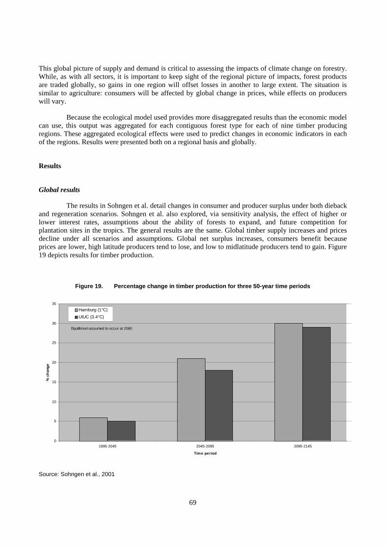
69
This global picture of supply and demand is critical to assessing the impacts of climate change on forestry. While, as with all sectors, it is important to keep sight of the regional picture of impacts, forest products are traded globally, so gains in one region will offset losses in another to large extent. The situation is similar to agriculture: consumers will be affected by global change in prices, while effects on producers will vary.
Because the ecological model used provides more disaggregated results than the economic model can use, this output was aggregated for each contiguous forest type for each of nine timber producing regions. These aggregated ecological effects were used to predict changes in economic indicators in each of the regions. Results were presented both on a regional basis and globally.
Results
Global results
The results in Sohngen et al. detail changes in consumer and producer surplus under both dieback and regeneration scenarios. Sohngen et al. also explored, via sensitivity analysis, the effect of higher or lower interest rates, assumptions about the ability of forests to expand, and future competition for plantation sites in the tropics. The general results are the same. Global timber supply increases and prices decline under all scenarios and assumptions. Global net surplus increases, consumers benefit because prices are lower, high latitude producers tend to lose, and low to midlatitude producers tend to gain. Figure 19 depicts results for timber production.
Figure 19. Percentage change in timber production for three 50-year time periods
0
5
10
15
20
25
30
35
1995-2045 2045-2095 2095-2145
Time period
% c
han
ge
Hamburg (1°C)
UIUC (3.4°C)
Equilibrium assumed to occur at 2060
Source: Sohngen et al., 2001
70
Global yields clearly increase over time because of two factors. First, climate change increases the annual growth of merchantable timber by increasing NPP. Second, the BIOME3 predicts a poleward migration of more productive species, which tends to increase the area of these more productive species.
However, while global forest yields rise, global temperatures appear to have a small effect on output. Both the Hamburg and UIUC models show comparable gains in yield at each time step, though their underlying global temperature predictions are quite different (approximately 1°C versus 3.4°C). There are significant differences between the two climate models in terms of regional and temporal temperature patterns. For instance, in the Hamburg scenario, production increases most heavily in low to midlatitude regions where climate changes are mild and growth is stimulated by increased carbon dioxide. In the UIUC model, production increases are similar for all regions. This pattern of regional differences between the two models continues and leads to the global aggregate trends depicted in Figure 19. One thing that is consistent is that when baseline conditions and time are held constant, the higher temperature scenario, UIUC, predicts slightly lower benefits than the low temperature Hamburg scenario. Our conclusions about the relationship between GMT and global forestry production are discussed below.
Regional results
While there are regional differences in how producers are affected, the pattern is different and more complex than in other sectors. Rather than facing losses, lower latitude producers are able to take advantage of climate change almost immediately, and expand short-rotation plantations. This expansion allows for higher production while world prices are close to baseline levels, just as other areas are experiencing dieback. In contrast, producers in mid- to high latitude regions are susceptible to the effects of dieback, and it takes many years before they experience growth increases because of their long-rotation species. Eventually though, this stock is replaced by more productive southern species and production increases, accompanied by a decline in world prices.
Main findings
We would expect the economic results for forestry to roughly track biophysical changes in terrestrial vegetation. When growth is estimated to increase, we would expect production to rise as well. If growth decreases at some point, production should too. This is the case in agriculture. Since we had only one forestry study to examine and taking into consideration the complexities of lags resulting from decadal long harvesting times, it is more difficult to draw a conclusion here. It does appear that everything else equal, both climate change scenarios in Sohngen et al. result in benefits, albeit the scenario with higher GMT has slightly lower benefits. This suggests, but does not confirm, that the relationship between GMT and global forest production is parabolic. Without more studies looking at wider range of climate changes, we cannot draw a definitive conclusion.
71
8. MARINE ECOSYSTEM PRODUCTIVITY
We examined one study that analysed changes in the production of marine ecosystems due to climate change: Bopp et al. (2001).
Choice of metric
Bopp et al. attempted to predict how climate change might affect marine primary production (production by marine plants, including phytoplankton and seaweeds). As with terrestrial ecosystem productivity, this one metric is limited and does not directly translate into fish productivity or changes in biodiversity. However, any changes in primary production would propagate up the marine food web and consequently indicate the possible effects of climate change on marine ecosystems in general. For instance, interannual variations in marine productivity due to El Niño can dramatically affect ocean fishery yields and the human populations that rely on them. Specifically, Bopp et al. estimated the change in marine export production, that part of the primary production that is transported below 100 m.
Scenarios
Bopp et al. considered a future of doubled CO2 and used the oceanic output (advection and eddy diffusion) from two different coupled atmosphere-ocean GCMs (LMD5 and Arpege). Their baseline climatology holds CO2 constant at 350 ppm, and the global warming scenario increases CO2 at 1% per year until reaching a doubling of CO2 after 70 years (they also consider a tripling and quadrupling of CO2 in a limited fashion, occurring at 110 and 140 years, respectively). The primary 2xCO2 model runs, however, extend to 80 years in the future. They did not provide a corresponding record of global average transient temperatures for the GCMs. Sea surface temperature, however, changes between 1.25°C and 1.5°C over the course of the experiment.11 The analysis did not account for changes in extreme events, variance, or a state change such as the breakdown of thermohaline circulation.
Models
Bopp et al. used the GCM outputs as input into two biogeochemical schemes, HAMOCC3 and P3ZD. Only the second biogeochemical scheme explicitly models plankton dynamics. The biogeochemical schemes are run off line.
Key factors and assumptions
Bopp et al. made several assumptions that bear noting. First, because their biogeochemical models were run off line, the analysis did not provide for feedback to the climate system from changes in the ocean’s biochemistry. In fact, the analysis did not allow them to distinguish dynamic from
11. At the time of this writing, we are unable to determine what change in global mean temperatures are associated
with these changes in sea surface temperatures.

72
biogeochemical effects. Second, the biogeochemical schemes they employed are grossly simplified in that they are phosphate based and lack limitation by other nutrients (e.g., Fe, N, Si). Finally, the models they employed do not account for competition between different species of plankton or that species abundance may change because of climate induced changes in ocean circulation or mixing.
Spatial scales and distributional issues
Overall spatial resolution was determined by the resolution of the constituent GCMs, 2° longitude x 1.5° latitude. The results were presented cartographically on the grid level and as zonal regional averages and global averages.
Results
We discuss the global and regional results under the same heading here because they are closely related in this sector.
Both combinations of models predicted similar responses to climate change. At 2xCO2 they predicted a 6% global decrease in export production, and showed opposing changes in the high and low latitude regions. In the low latitudes, climate induced changes in the ocean decreased export production by 20%, but increased export production 30% in the high latitudes. Reductions in low latitude export production are located primarily in the Indian Ocean, Tropical Atlantic, and Western Pacific. Examining the results in the economically important fisheries region of the equatorial Pacific indicates that export production decreased by 5 to 15%. In general, changes in production are driven by reduced nutrient supplies in the low latitudes and an increased light efficiency in the high latitudes due to a longer growing season. Both changes result from increased stratification in the upper ocean. Despite the general concordance of the two models, there are substantial regional discrepancies.
Results were not reported for lower levels of climate change, so it is not possible to determine if global export production declines at smaller increments of increase in global mean temperature.
Other factors
Reducing uncertainties in ocean dynamics is a crucial first step to improving estimates of the impact of climate change on marine productivity. The Southern Ocean is particularly sensitive to such uncertainty, and improving forecasts for this important region will also rely on better higher resolution models and better sea-ice models. Explicit inclusion of other nutrients in biogeochemical models will lead to improvements in the future.
Main findings
With only one study containing few data points, it is difficult to draw conclusions about how marine ecosystem productivity is related to increased GMT. Clearly, at some point, increasing GMT leads to reduced marine ecosystem productivity. It is reasonable to assume that further increases in GMT lead to further decreases in productivity, but we are uncertain about the relationship between GMT and marine ecosystem productivity for temperature changes less than those considered by Bopp et al.

73
9. BIODIVERSITY
We examined one study that informs speculation regarding the impacts of climate change on global biodiversity: Halpin (1997).
Choice of metric
Estimating the impacts of climate change on the global abundance and distribution of biodiversity is a tall, if not impossible, order. Halpin took on this task in an indirect matter. He hypothesised that the survival and distribution of terrestrial plant and animal species depend on the distribution of the climates on which they depend. Specifically, Halpin examined the potential threat climate change poses to global nature reserve systems, the repositories of significant biodiversity. Since climate change affects the distribution of climate zones, species may move within or beyond the confines of existing nature reserve boundaries. Halpin estimated the percentage of biosphere reserves that might experience a significant change in “ecoclimatic class” as well as the global average change for all terrestrial areas. A change from a current ecoclimate class to a different class was interpreted as a significant climate impact for a reserve site.
Gitay et al. (2001) noted that this approach contains many limitations and in particular cautioned against identifying species-specific impacts. While the approach used by Halpin estimates long-term changes, biomes experiencing changed climate may be able to tolerate new conditions. However, even if habitat survives changes in climate, the migration of new species into a region and the subsequent competition may mean that biomes are changed fundamentally.
Scenarios
The four GCMs used in Halpin’s analysis were run for a doubled CO2 scenario. As with other studies using this battery of GCMs, equilibrium was presumed to occur at 2090. The associated temperature changes are shown in Table 3. Since the scenarios are equilibrium and not transient, impact trends according to temperature were deduced via cross-model comparison.
Models
Halpin compared current climate data bases and modified climate grids. He used a 19 class, aggregated ecoclimatic structure for the world. The current ecoclimatic classes of the UNESCO biosphere reserves network (MAB-UNESCO, 1990) were compared to the ecoclimatic projections generated by the UKMO, GISS, GFDL, and OSU GCMs.
The analysis predicted sites where the climatic change falls within the existing climatic range of the bioreserve and sites where the projected change exceeds the current range. It was presumed that biodiversity in reserves that have a change in climate will be threatened.
74
Spatial scales and distributional issues
Halpin presents results on both global and zonal bases.
Key factors and assumptions
This sort of geographic assessment makes no attempt to predict the specific biotic outcomes of projected changes for the particular species composition contained with the reserves. A multitude of factors that are ignored will influence actual outcomes. For example, the study did not address how biodiversity will be threatened. Will change in climate exceed climatic tolerances of species, allow other species better suited for the new climate to migrate into the reserve and outcompete the current occupants, or lead to disturbance? One important consideration, however, that was not investigated, and on which the ability of actual species to migrate or adapt to climate change will depend, is rates of change. Species may well be able to migrate along with ecoclimatic zones or may be able to adapt to new ecoclimatic classes. However, it is likely that the rate at which ecoclimatic zones migrate may control both abilities. Furthermore, human development and other topographic boundaries can limit or impede migration by imposing barriers. This could particularly be the case with reserves. At a minimum, this approach indicates the potential for climate change to introduce risks to biodiversity.
Results
Because global results are closely linked to regional results in this sector, we discuss them together.
Figure 20 displays the frequency with which biosphere reserves and terrestrial area in general experience a change in ecoclimatic class as a function of temperature. With the exception of a hitch around a 4°C change, presumably due to the difference in precipitation between GISS and GFDL, the trend is generally increasing and linear. While the GCM scenarios project major changes in the distribution of ecoclimate classes at a global scale, the more important point is that the frequency of ecoclimatic impacts on reserve areas is generally higher than the global averages. Halpin suggested a fairly straightforward explanation. The global distribution of reserves has a northern spatial bias, because of the greater abundance of land mass at northern latitudes and the fact that northern industrialised nations maintain more reserve sites. This bias coincides with the larger magnitude climate impacts projected by the GCMs that Halpin used. This produces higher rates of climate change for reserve sites than the average for terrestrial areas.

75
Figure 20. Percent change in ecoclimatic classes for biosphere reserves compared to global average
0
10
20
30
40
50
60
70
80
90
0 1 2 3 4 5
°C
% o
f are
a w
here
ec
o-cl
imat
ic c
las
s ch
ang
e o
ccu
rs
Biosphere Reserves
Total Terrestrial Area
OSU
GFDL
GISS
UKMO
Source: Halpin, 1997
Other factors
Future studies could improve on this analysis by investigating shifts in ecoclimatic class under transient climate change scenarios, giving important insight into rates of climate change and the ability of species to adapt or migrate. Those studies could also attempt to better assess the consequences of changes in ecoclimate zones. Future studies must also do a better job of characterising and exploring dispersal mechanisms and barriers to migration, which might be geophysical (including fragmented habitat in general), climatic, or ecological (competition).
Main findings
It seems highly likely that larger increases in GMT this century will result in more losses of biodiversity, for two reasons. Many species may be able to tolerate a certain level of change in climate, but at higher levels of change, these thresholds will be exceeded. Higher GMTs also mean faster rates of change in climate, which will exceed the ability of increasing numbers of species to adapt. In addition, the threat to biodiversity from climate is much larger when considered in conjunction with the pressures of development. Habitat fragmentation and pollution among other factors already threaten many species. In combination with climate change, the loss could be larger. The IPCC concluded, “There is little evidence to suggest that processes associated with climate change will slow species loss” (Gitay et al., 2001; p. 250). We are highly confident that biodiversity will decrease with increasing temperatures; what is uncertain is whether there is a straight line relationship or exponential relationship between higher GMT and loss of biodiversity.
76
10. ENERGY
We are aware of only one study that estimated the effects of climate change on the demand for global energy: the energy sector analysis of Tol’s (2002b) aggregate study (discussed in Section 11). Tol followed the method of Downing et al. (1996). Climatic change is likely to affect the consumption of energy via changes in the demand for space heating and cooling. As global temperatures rise, the global demand for heating is likely to decrease, while the demand for cooling is likely to increase. Tol relied on Downing et al.’s global study, which in turn extrapolated from a simple country-specific (United Kingdom) model that relates the energy used for heating or cooling to degree days, per capita income, and energy efficiency. Economic impacts were derived from energy price scenarios and extrapolated to the rest of the world. Tol also reported that Downing et al. argued that the demand for heating decreases linearly as temperature increases. They also assumed that virtually all homes and buildings that need heating have it. Energy efficiency was assumed to increase over time.
In developing a model for the demand for cooling energy, Downing et al. assumed demand for cooling to increase roughly linearly with temperature. Air conditioning was assumed not to have saturated all buildings and homes that could use it. As with the model for heating energy, demand for cooling was assumed to increase with population. Again, efficiency gains reduce the costs.
Results
According to Tol’s best guess parameters, by 2100, benefits (reduced heating) are about 0.75% of GDP and damages (increased cooling) are approximately 0.45%. The global savings from reduced demand for heating remain below 1% of GDP through 2200. However, by the 22nd century, they begin to level off because of increased energy efficiency. For cooling, the additional amount spent rises to just above 0.6% of GDP by 2200. Thus throughout the next two centuries, net energy demand decreases. Tol, however, did not report how temperature changes over this period, so we cannot associate a particular level of net benefits with a given temperature. Despite the results at 2200, it is reasonable to assume that at high enough levels of temperature change, the increased spending on cooling will come to dominate the savings from reduced expenditure on heating.
Main findings
We are highly confident that global energy use will eventually rise as global mean temperature rises, but we are not certain about whether a few degrees of warming will lead to increased or decreased energy consumption. With higher temperatures, demand for heating decreases and demand for cooling increases. One can imagine that a curve relating energy demand to mean global temperature might be shaped like “U” or a “V” (Figure 21). An important question is whether we are to the right of the low point of such a curve (where further increases in temperature increase total demand), in which case global energy consumption will rise with higher GMT, or whether we are on the portion of the curve that foretells decreasing demand (left of the low point), in which case global energy consumption will first decline and then eventually rise as GMT increases. Tol’s analysis suggests that we are can still look forward to reductions in total consumption. However, Mendelsohn’s (2001) analysis of the United States finds that

77
energy costs will increase even with an approximate 1°C increase in GMT. Since the United States consumes about one-fourth of global energy, this may be indication that global energy demand will increase immediately as temperatures rise. Thus, based on the limited literature, we are unable to determine the effective shape of the damage relationship we face. We consequently conclude that we are uncertain about the relationship between energy demand and increased GMT.
Figure 21. Idealised annual energy demand versus mean temperature
Total energy demand
Low point in energy use
Temperature

78
11. AGGREGATE
We briefly examined two aggregate studies that analysed the global impacts of climate change across a number of sectors. As with the individual sectors, we discuss the methods used, basic assumptions, and results for each study. The two studies we examined are Tol (2002a, 2002b) and Nordhaus and Boyer (2000).
Tol’s study considered impacts of climate change on agriculture; forestry; species, ecosystems, and landscapes; sea level rise; human health; energy consumption; and water resources. It omitted impacts related to amenity values, recreation, tourism, extreme weather, fisheries, construction, transport, energy supply, and morbidity. Tol derived estimates of the impacts of climate change from the literature. He limited consideration to those studies that are both globally comprehensive and based on climate scenarios generated by GCMs. The meta-analysis ties impacts to changes in global mean temperature and splits the world into nine regions. He conducted both a static analysis of the impacts of a 1°C change in global temperature on the present situation and a dynamic estimate of the potential impacts over the 2000-2200 period, taking into account the vulnerability of regions to impacts (changes in population, economies, and technology are considered, although uncertainties about these scenarios are ignored). Tol manipulated the results of published studies to match his regions, and scaled their results to correspond to the 1°C change he examined. He also adjusted the results of some studies to make assumptions regarding adaptation consistent. In some cases, he also modified results to capture other dimensions of impacts that the original studies did not (e.g., inclusion of forced migration costs as part of sea level rise study results). During this process he made several broad assumptions, one of which is that regions are homogenous. Expanding his analysis to one that is dynamic necessitated adopting many more assumptions and extrapolating, by means of statistical methods, his static findings over different climates and different vulnerabilities to climate change. The necessary parameters were estimated from the underlying literature or guessed. He did, however, conduct a sensitivity analysis of key parameters to determine the effect of his choice of parameters.
Tol’s results show that the impacts of climate change can be positive as well as negative, depending on the sector, region, or time period at which one is looking. The impact on overall welfare depends on how one decides to aggregate results. Aggregating results across regions, even when results are expressed in monetary fashion as they are in Tol’s analysis, is problematic. Statistical lives, for instance, may be valued differently in different regions, and thus different weights could be assigned to the results for each region according to a chosen indicator. Tol aggregates static results both as simple sums and in an equity weighted fashion, where income determines the weighting factors. The simple sum results in a 2.3% increase in income globally. The equity weighted sum reduces this figure to 0.2% of income.
Regional aggregate impacts can differ substantially from global aggregate impacts and from region to region. Especially at low magnitudes of climate change, results are likely to be mixed across regions. For an increase of 1ºC in global mean temperature and a .2 meter sea level rise as above, impacts in the OECD, Central and Eastern Europe, the former Soviet Union, the Middle East, and China are on balance positive. In all other regions, impacts are on balance negative. At low levels of climate change most developing countries, especially those in the low latitudes, are negatively impacted. Table 7 presents Tol’s results for a

79
benchmark 1ºC change. Other studies such as Nordhaus and Boyer (2000) estimate different regional results.
Table 7. Annual impact of a 1ºC increase in GMT - change in Gross Domestic Product
Regions Billion of dollars Percent of income
OECD-America (excluding Mexico)
175 (107) 3.4 (2.1)
OECD-Europe 203 (118) 3.7 (2.2) OECD-Pacific (excluding S. Korea)
32 (35) 1.0 (1.1)
Central and Eastern Europe and former Soviet Union
57 (108) 2.0 (3.8)
Middle East 4 (8) 1.1 (2.2) Latin America -1 (5) -0.1 (0.6) South and South East Asia -14 (9) -1.7 (1.1) Centrally Planned Asia 9 (22) 2.1 (5.0) Africa -17 (9) -4.1 (2.2)
Aggregate Estimates
(i) Simple sum 448 (197) 2.3 (1.0) (ii) Average value -522 (150) -2.7 (0.8) (iii) Equity-weighted sum 40 (257) 0.2 (1.3)
Notes: Figures in parenthesis are the standard deviation of the mean. Dollars are 1990 US dollars. Positive values are benefits and negative values are damages. The last three rows represent three different approaches to aggregation and lead to very different outcomes. The simple sum (i) approach is output based and constructed from the individual regional estimates which use different monetary values for different impacts. This approach ignores disparities between the regional estimates. Average value (ii) approach uses globally averaged prices to value non-market goods and services. The sign switch between the simple sum and average value aggregates is largely due to the valuation of mortality where using world average values rather than regionally differentiated values place the emphasis on the increase in mortality in developing countries, compared to the decrease in mortality in the OECD. The equity-weighted sum (iii) approach uses the ratio of global to regional income per capita as an equity weight. The difference with simple summation is due to higher weights for the poorest regions which tend to have relatively higher level of negative impacts compared to other regions. Source: from Tol (2002a) The picture of dynamic results is also mixed (Tol, 2002b). There are both positive and negative impacts for different regions at different points in time. Dynamic results are not aggregated globally. For the OECD countries, Tol predicts that the overall impact of climate change over the next two centuries will be positive, though the complete time series begins and ends with predicted damages. The overall results for Latin America are similar, as are those for the Middle East and Centrally Planned Asia. However, the entire curve is shifted closer toward damages for the last two regions. The impacts of climate change on South and Southeast Asia, Central and Eastern Europe, and the former Soviet Union are on the whole negative. All results for Africa are negative. By the end of the analysis period, 2200, annual results for all regions are negative, with the exception of the Middle East and Centrally Planned Asia. Clearly, results at the regional level tell a different story, than global results do, in terms of impacts as a function of time and similarly, in terms of sensitivity of impacts to temperature.
Nordhaus and Boyer’s aggregate analysis relied on an integrated model, the Regional dynamic Integrated model of Climate and the Economy (RICE). Global impact is derived from regional impact

80
estimates. RICE includes eight regions, though for their analysis Nordhaus and Boyer divided these eight regions into 13 subregions. Climate change is represented by global mean surface temperature. The study is dynamic and results are derived first for 2.5°C of change (the average change corresponding to a doubling of CO2 from three climate scenarios considered). Damage functions are then inferred that extend the analysis to 6°C of warming. The model takes a willingness-to-pay approach, estimating the insurance premium different societies are willing to pay to prevent climate change and its associated impacts. Parameters are estimated based on existing studies, modification of existing results, guessing, and survey results. The Nordhaus and Boyer analysis is unique among aggregate studies in its attempted inclusion of nonmarket and potential catastrophic impacts as well as market impacts. The study estimated impacts in agriculture, sea level rise, other market sectors, health, nonmarket amenity impacts, human settlements and ecosystems, and catastrophic events.
Nordhaus and Boyer presented aggregate damage curves for regions and by weighted summation, where weights are based on population or projected 2100 regional output (Figure 22).
Figure 22. Regional damage functions
Source: Nordhaus and Boyer, 2000
The impacts of a 2.5°C warming range from benefits of 0.7% of output for Russia to net damages of almost 5% for India. The global average of damages for a 2.5° warming is 1.5% if weighted by output or

81
1.9% if weighted by 1995 population.12 One important distributional result is that low income areas, India and Africa in particular, and Europe are subject to significant damages over the next century. For most countries, market impacts are small in comparison to the possibility of potential catastrophic impacts. The large uncertainty associated with these catastrophic impact estimates implies that there is great uncertainty associated with the overall results. Nordhaus’ and Boyer’s results also demonstrate that the method of spatial aggregation has an important effect not only on the total magnitude of global climate change impacts, but also on the contribution of particular sectors to that total (Figure 23).
Figure 23. Global impacts in different sectors and according to method of aggregation
-0.5
0
0.5
1
1.5
2
2.5
Aggregation method
Per
cen
t o
f G
DP
Catastrophic impact (2.5 degrees)
Settlements
Nonmarket time use
Health
Coastal
Other vulnerable market
Agriculture
Aggregated by Output
Aggregated by Population
Notes: Estimated aggregate impacts at 2.5 o C change in global mean temperature. Sectors placed above the 0% of GDP line show damages (of positive magnitude). Sectors below the 0% of GDP line are benefits or negative impacts; which in this case is Nonmarket time value. Total global damages are not explicitly indicated, but can be computed by subtracting benefit categories from total damages, that is, benefits below the x-axis from those above. The net effect based on the output aggregated approach is a damage of 1.5% of GDP. For the results weighted by population, Nordhaus and Boyer (2000) report a global total of 1.88% of GDP. However, when the population-weighted aggregated sectoral results presented above are totaled, the present authors arrive at 2.2% of GDP. Population weighted global average is weighted according to population in 1995. Output weighted global averages are weighted by projected output in 2100. Finally, nonmarket time use generally refers to the estimates of the value of the total time people spend on climate sensitive recreational activity, which Nordhaus and Boyer estimate increase with higher levels of climate change.
12 For the results weighted by population, Nordhaus and Boyer (2000) report a global total of 1.88% of GDP.
However, when the population-weighted aggregated sectoral results presented above are totaled, the present authors arrive at 2.2% of GDP.

82
For instance, aggregating by output gives more weight to impacts in developed countries .This results in more benefits compared to population weighted impacts in the case of non-market use time. Weighting by population tends to emphasize impacts in populous developing countries and especially the contribution of vulnerable sectors such as health to the aggregated total. The net effect is that weighting by output results in smaller damages than weighting by population.
Main findings
The few studies on aggregate impacts of climate change consistently estimate that there will be damages beyond approximately 2 to 3°C of increase in GMT (Figure 24).
Figure 24. Estimated aggregate global damages
-11
-10
-9
-8
-7
-6
-5
-4
-3
-2
-1
0
1
2
3
0 1 2 3 4 5 6
Global Mean Temperature (°C)
Per
cent
of
Wor
ld G
DP
)))
Mendelsohn, output
Nordhaus, output
Nordhaus, population
Tol, output
Tol, equity
Note: The aggregate data presented in this graph varies in a number a ways between studies. For example, with respect to the coverage of non-market impacts, such as impacts on ecosystems and human health Tol’s figures include estimates of ecosystem damages using gross estimates of willingness to pay to preserve ecosystems. He also provides estimates of the value of loss of human life. In contrast, the Mendelsohn and Schlesinger’s figures omit non-market damages entirely. Nordhaus and Boyer on the other hand, include estimates of catastrophic damages based on willingness to pay to avoid extreme events, value of loss of human life, amenity values associated with climate, and value of time (e.g., recreation). The other studies do not include these categories of impacts. However, Nordhaus and Boyer do not directly estimate value of ecosystem impacts (e.g., willlingness-to-pay to protect endangered species) as Tol does. Source: Smith et al. 2001, citing Mendelsohn and Schlesinger 1999; Nordhaus and Boyer 2000; Tol 2002b
Damages are estimated to continue increasing at higher increases in temperature. Where there is disagreement among the studies concerns what happens for smaller increases in GMT. Some studies show net benefits for a small amount of warming, while Nordhaus and Boyer show damages at such levels.

83
Thus, the aggregate studies do not present consistent results concerning the shape of the damages curve, but do consistently show increasing damages at higher magnitudes of climate change. For a few degrees of increase in mean global temperature, aggregate impacts appear to be uncertain.

84
12. DISCUSSION
This section discusses the main findings of our survey of the literature on global sectoral studies. We did not attempt to aggregate the results from various studies and sectors but assessed whether there are consistent patterns of relationships between impacts and GMT. We then examined the uncertainties associated with these studies, and whether they have adequately and appropriately accounted for factors that can substantially affect estimates of impacts. We also looked at related topics, including choice of metrics, time scales, spatial and distributional issues, proactive adaptation, and ancillary benefits. The section concludes by making some recommendations on research needs.
Total impacts
Given the state of knowledge on how impacts in specific sectors change as GMT increases, what are the total impacts across sectors from climate change as a function of increasing GMT?
Determining total impacts would be trivial if all of the impact studies used the same metric. If all impacts were measured in dollars, number of lives affected or some other common metric, we could simply sum the numbers from individual sector studies.13 However, even with a common metric, we would encounter the sorts of stumbling blocks outlined in the introduction. Simple summation of monetized impacts across regions or sectors would give the wealthy more weight than the poor. The use of people at risk or lives affected could overstate the true impacts because some people may be affected in more than one sector. Since the studies we reviewed use different metrics, we cannot aggregate results; nor do we attempt to transform results presented in one metric to another in order to do so.
Instead, we looked for common patterns between the damage relationships presented for different sectors. Do impacts increase as temperatures rise, are there thresholds, does the sign of impacts reverse as temperature rises (parabolic), or is the relationship indeterminate? Table 8 summarises the patterns in the studies we examined by sector, and the most obvious conclusion is that there are different relationships between impacts and temperature across the sectors.
13. In reality, even with the benefit of a common metric, simply summing damages from various sectors would not be
entirely accurate. Such an approach would still not account for important interactions between sectors and would omit sectors for which there are no estimated global impacts, such as migration.

85
Table 8. Summary of sectoral damage relationships with increasing temperature
Sector Increasing adverse
impactsa Parabolic Unknown
Agriculture X
Coastal X
Water X
Health Xb
Terrestrial ecosystem productivity
X
Forestry X?c
Marine ecosystems X?d
Biodiversity X
Energy X
Aggregate X
a. Increasing adverse impacts means there are adverse impacts with small increases in GMT, and the adverse impacts increase with higher GMTs. We are unable to determine whether the adverse impacts increase linearly or exponentially with GMT. b. There is some uncertainty associated with this characterisation, as the results for the studies we examine are inconsistent. On balance, we believe the literature shows increasing damages for this sector c. We believe this is parabolic, but with only one study it is difficult to ascertain temperature relationship, so there is uncertainty about this relationship. d. This relationship is uncertain because there is only one study on this topic.
Some of the sectors exhibit increasing adverse impacts with increasing degrees of climate change. Since the data reported in the studies are limited, we were generally unable to determine if these relationships are linear or exponential. None of sector-specific relationships appear to be characterised by thresholds below which there is no impact. Some sectors are characterised by a parabolic relationship between temperature and impacts, and for the others, the relationship is unknown.
There appear to be increasing adverse impacts with higher GMT in the coastal resources, marine ecosystems, human health, and biodiversity sectors. It is highly probable that adverse impacts in the coastal and biodiversity sectors will rise with increasing magnitudes of climate change. This confidence arises not only from an examination of the aforementioned studies but also from an understanding of the exposure and sensitivity of these systems. We are less certain for human health and marine ecosystems.
The results for the studies on human health are not entirely consistent. Furthermore, there are real questions as to how to aggregate results and if doing so is possible at all, since different health threats reflect different types and degrees of risk. On balance, though, these studies and our knowledge of the sector do seem to suggest the possibility of increasing risk with increasing GMT.
The information on marine ecosystems is limited. We presume that marine ecosystem productivity will continue to decline as temperatures move beyond those considered in the one published study on this topic. Whether there are reductions in productivity (net adverse impacts) at lower levels of temperature or gains (net benefits) is uncertain. We do not have enough information to determine whether

86
there adverse impacts right from the start or if there is a parabolic relationship with increasing GMT. Furthermore, there are no global studies that quantify how decreased marine primary productivity might affect the rest of the food chain.
There appears to be a parabolic relationship between impacts and GMT for terrestrial ecosystem productivity and agriculture. The terrestrial ecosystem productivity studies consistently estimated increased productivity at small magnitudes of climate change, but decreased productivity at larger magnitudes. The relationship between impacts and temperature in agriculture is somewhat less consistent from study to study, but nonetheless seems to be parabolic. Some of the studies we reviewed estimated benefits from small increases in GMT (Rosenzweig et al., 1995 and Darwin et al., 1995), while one showed adverse impacts (Parry et al., 1999). All three agriculture studies estimated reduced global production (i.e., adverse impacts) beyond an approximate 3 to 4°C increase in GMT. Both the White et al. (1999) and Cramer et al. (2001) studies of terrestrial ecosystem productivity clearly indicate that initial gains in productivity are followed by reductions; the relationship between terrestrial ecosystem productivity and GMT is likely to be parabolic.
The Sohngen et al. (2001) study of forestry indicated a slight negative effect of relatively higher temperatures. Since both scenarios in the study considered estimate net increase in forest production and the warmer scenario shows a slight reduction in benefits, the relationship between GMT and production may be parabolic. However, the results are complicated by factors (including time lags) that make it difficult to determine the underlying relationship between increases in GMT and forestry impacts in this study. Yet the fact that the terrestrial vegetation productivity studies point to a parabolic relationship, and that economic output should move consistently with biophysical change, indicates that forestry is likely to have a parabolic relationship with temperature. We think the relationship is parabolic, but put a question mark in Table 8 because the literature on global forest production and climate change is limited.
The relationship between impacts and change in climate is clearly uncertain for a number of sectors that are sensitive to climate. This is particularly true for water resources, for which it is hard to determine whether impacts increase or decrease.
Our conclusions regarding energy are based on only one study, Tol’s reanalysis of the work by Downing et al. (1996); other studies indicate that results could be different. Consequently, we cannot determine with any certainty what the next few degrees of warming will bring.
What does this mean taken together? Since the different sector studies do not show a consistent relationship, it is not possible to draw a conclusion about whether impacts generally increase as temperature rises or whether there is a parabolic relationship. Given the fact that several studies show some impact with even small amounts of temperature change, we can rule out the threshold relationship. Beyond an approximate 3 to 4°C increase in global mean temperature, all of the studies we examined, with the possible exception of forestry, show increasing adverse impacts. In total, it appears likely that there are increasing adverse impacts beyond this level. However, the relationship between total impacts and climate change up to a 3 to 4°C increase in GMT remains uncertain. Not only is the shape of the curve uncertain, but whether it lies above or below the adverse impacts/benefits line or traces it between 0°C and 3 to 4°C is also uncertain.
It is interesting to consider whether the studies of aggregate impacts give us any additional insight. Examination of Figure 24 reveals that beyond approximately the same threshold of 3 to 4°C, the aggregate studies tend to find that there are increasing net damages. Below approximately 3 to 4°C, the studies diverge. Mendelsohn and Schlesinger (1999) and Tol (2002b) estimated initial net benefits, which peak and then decline. Nordhaus and Boyer estimated damages from the start, which then increase exponentially with temperature.

87
In summary, the literature shows that for increases in GMT between 0°C and 3 to 4°C, the relationship between impacts and temperature is uncertain. Beyond this point, the studies generally estimated net adverse impacts that increase as GMT increases.
Uncertainties
How certain are we of this conclusion? There are two main considerations in assessing our uncertainty: how comprehensive our analysis was and how thorough the studies that we examined were. The critical question is whether any uncertainties could be large enough to change our estimate of the shape of the curve or the increase in GMT beyond which there clearly are adverse impacts.
The survey found several potentially important sectors for which the relationship cannot be determined or has not been studied: we cannot determine how impacts in the water, health, and energy sectors change with GMT. Furthermore, there are no published studies on how global tourism and recreation expenditures will change as a result of climate change. This is a large sector; 7% of the U.S. GDP is derived from tourism (U.S. BEA, 2002). A large reduction or increase in tourism and recreation expenditures could have a substantial impact on the aggregate economic consequences of climate change. Tourists might shift away from activities and areas adversely affected by climate change (e.g., skiing or coastal areas inundated by sea level rise or impacted by cyclones) toward activities or areas made relatively more favourable by climate change. There are likely to be some changes in total expenditures as well overall welfare derived from these activities.
The more difficult question to address is whether the studies that were surveyed provide a solid enough foundation on which to base a conclusion. Have they appropriately addressed or neglected important factors that could substantially change or even reverse the results?
There are a number of important sources of uncertainty underlying the estimates, and six are addressed below: change in variance of climate, adaptation, development, long-term temperature changes, change in the climate system, and interactions among sectors.
Change in variance of climate
Many critics of the current generation of global impact studies point out that the bulk of these studies assume a change only in average climate and do not address changes in climate variance or extreme events (e.g., Schneider et al., 2000b). To be sure, changing mean conditions does capture some change in extreme events. For example, imposing an increase in precipitation of 10% on the historical record (which is done in most impact studies) increases all precipitation events by 10%. So, the wettest periods would be 10% wetter. Furthermore, the frequency with which extreme events of a certain magnitude occur would increase simply with a change in mean climate and no concomitant change in variance. But this approach does not capture potential changes in the magnitude of variance and can be particularly misleading if the observed climate period used in the analysis is a relatively stable one.
Change in variance is plausible and has already been observed to some extent. Easterling et al. (2000) found that extreme precipitation increased over the 20th century. Variance in the future could change as well. Timmerman et al. (1999) found that El Niño conditions could become more frequent and interspersed with stronger La Niñas, although the IPCC was equivocal about whether the intensity or frequency of El Niño Southern Oscillations would increase. Climate models generally find that precipitation intensity will continue to increase (Houghton et al., 2001).

88
It is difficult to say whether an increase in variance would reverse or amplify the overall findings discussed above. The few studies that have addressed this possibility do not provide consistent results. Chen et al. (2001) examined how a change in ENSO as modelled by Timmerman et al. could affect U.S. agricultural output. The estimated impacts are negative (about $1 billion in losses), but are about an order of magnitude smaller than the impacts of a mean change in climate (NAST, 2000). On the other hand, Frederick and Schwarz (1999) found that the magnitude of economic impacts of a severe drought in the United States could be $100 billion per year. It is not clear how the drought modelled by Frederick and Schwartz differs from historic droughts. This level of damages is comparable to or even greater than the total potential economic gains of climate change for the United States for a limited amount of warming (although severe droughts are discrete events while estimates of gains from a change in long-term mean conditions are annual average gains sustained over long periods) (e.g., Mendelsohn and Neumann, 1999).
Adaptation
Quantitative impact studies make simple assumptions about adaptation. Some assume specific adaptations are made, such as changing planting dates or building sea walls. Others rely on spatial analogy, assuming that people in one location will adopt the same practices used by people in locations with climates that are similar to what their future holds. The studies that assume specific adaptations probably underestimate the changes people will make. Studies that rely on spatial analogy do not address the impediments and costs that may be involved in adopting practices from other regions. Assumptions about adaptation can substantially affect results, as Rosenzweig et al. (1995) demonstrate.
It is difficult to know or predict exactly how affected parties will react. Smit et al. (1996) and West and Dowlatabadi (1999), among others, point out the complexities involved in adaptation. Furthermore, it is one thing to adapt to a gradual and monotonic change in climate — it may be far more challenging to adapt to a rapid change in climate or one that involves increased variance. Indeed, studies of adaptation to climate variance (e.g., Glantz, 1988) demonstrate that affected parties may react too quickly to short-term variance, neglecting the potential for reversals of climate. For example, residents of the Great Lakes built structures closer to receding shorelines during low level periods of the early 1980s, only to witness flooding of those structures as lake levels rose (Changnon, 1997).
A realistic consideration of adaptation could lower some of the thresholds at which adverse impacts are generally estimated to occur.
Development
A critical uncertainty affecting our determination of how vulnerable systems are to climate change relates to assumptions various studies make regarding development. If we impose climate change on today’s society, vulnerability will be greater than if we assume increases in income and improvements in technology in the future. For example, Tol and Dowlatabadi (2002) concluded that large increases in income could substantially reduce the vulnerability of people in developing countries to climate change induced malaria mortality.
����������������� ��������������������������������������������������������������� �������Swart, 2000) all assume increased income per capita, across the globe. Will this happen? While global income rose in recent decades, and some countries such as South Korea made spectacular gains in income, other parts of the world, such as much of Africa, have experienced no growth and even reductions in income. Indeed, there may be more uncertainty about future socioeconomic conditions than about future climate conditions.

89
Another key uncertainty regarding development concerns technological progress. Assumptions about changes in technology can dwarf assumptions about the effects of climate change. Will past progress continue into the future, or even accelerate? This is critical in sectors such as agriculture. If the gains in productivity in agriculture reaped in the last half of the 20th century continue, global production will increase tremendously. There could be large surpluses, allowing sufficient cushion to absorb potential reductions due to climate change. Can these gains be sustained? Are there biophysical limits or other reasons why the gains may level off?
In addition, development can affect thresholds. For example, the IPCC concluded that warming above 3°C will reduce crop yields (Gitay et al., 2001). This is based on current climate tolerances of crops. However, it is uncertain whether agricultural research can increase the temperature threshold that crops can tolerate. If it does and new cultivars are developed and diffused to farmers, agriculture may be able to withstand even higher levels of climate change before production is reduced. Such considerations could increase some of the thresholds at which adverse impacts are estimated to occur.
Long-term temperature changes
The studies we considered examined changes in the 21st century. As Houghton et al. (2001) point out, it is highly likely that climate will continue changing into the 22nd century and even beyond. Even aggressive greenhouse gas stabilisation measures will still result in long-term change in climate. Although the rate of climate change will begin to slow down, additional warming thresholds will be crossed, potentially resulting in additional adverse impacts. Those additional impacts are not accounted for in this study, and thus the long-term consequences of different levels of increase in GMT may be underestimated. This may be particularly significant for coastal resources because of the long-term inertia in the climate-ocean system.
Change in the climate system
Global warming in the 21st century could trigger fundamental and potentially catastrophic changes in the climate system that may not be realised until after the 21st century. These events might include a slowdown or complete breakdown of the thermohaline circulation, which could result in cooling of the North Atlantic, including Western Europe and eastern North America (Vellinga and Wood, 2002); melting of the West Antarctic Ice Sheet; or a runaway greenhouse effect. The magnitudes of change required to trigger catastrophic events are uncertain. Larger changes in GMT than are likely to occur in this century would be necessary to trigger many of these events. Our survey did not consider the consequences of such events or the probabilities of triggering them, and thus may underestimate long-term adverse impacts associated with particular increases in global mean temperature.
Interactions among sectors
The sectors addressed in this study are not isolated in reality. Water and agriculture are one example of closely linked sectors. Decreased water supplies can limit agricultural production, while increased agricultural demand for water puts more pressure on water supplies. Other sectors exhibit similarly tight links. Indeed, none of the sectors studied is unaffected by changes in any of the other sectors. These linkages might result in exacerbation or, in some cases, amelioration of impacts we report. Thus, thresholds or slopes of damage curves might be higher or lower depending on these linkages.
The studies we considered generally did not consider linkages with nonclimate stressors. Factors such as pollution, habitat fragmentation, and population growth can increase the sensitivity of many of
90
these sectors to climate change. Depending on the sector, development can serve as an additional stressor or can help ameliorate climate related impacts.
Finally, few of the studies we examined addressed whether adverse impacts across sectors might lead to societal disruptions such as migration or conflict (Nicholls et al., 1999, for one, assumed people will migrate out of the coastal zone if there is continued flooding). It is difficult to simulate these events because they can be the result of many factors. Nonetheless, it is possible that such events might happen. Not considering them probably biases results toward an underestimate of impacts.
Other issues
Other issues important to assessing the credibility and utility of the literature reviewed in this study include the choice of metrics, temporal scales, and range of climate change addressed, and spatial and distributional issues. Two issues that the paper or studies we examined do not consider explicitly are proactive adaptation and ancillary benefits.
Use of metrics
This study used metrics as reported by the authors. Those metrics are quite varied, and include dollars, number of people affected, change in “ecoclimatic” zone, and ecological measures such as net ecosystem productivity. Since these are distinct metrics, it is not possible to combine them without converting them to a common unit. Some authors such as Nordhaus and Boyer (2000) used monetary units, while Arnell et al. (2002) primarily used number of people at risk (although they use different measures for ecosystem productivity).
There is no right or wrong approach when it comes to metrics (see Schneider et al., 2001, for more discussion on the use of metrics). It is important that metrics be acceptable and meaningful to users of the information, such as policy makers. Using a common metric has the advantage of enabling analysts to sum sectoral results and report a total damage result. But metrics that facilitate summation may not always be appropriate or meaningful for all sectors. For example, while it can provide useful information, relying on willingness to pay to avoid adverse ecological impacts is controversial and may not be meaningful to many readers. If such measures are not broadly acceptable or meaningful, it is not clear how results can aid policy makers.
We believe that there is value in reporting results based on different metrics and ascertaining whether the patterns of impacts are consistent or inconsistent. Where common metrics such as dollars are used across studies, results can be combined. Where different metrics are used, results should be displayed separately. Readers will need to make their own judgements about comparability or tradeoffs that result from choice different metrics.
There is also value in using multiple metrics to cover the same set of impacts. Expressing all impacts in terms of dollars allows for combining results across sectors. It also measures the degree of impact. But such a metric effectively weights the impacts to the rich more than it does the impacts to the poor. Most of the world’s population lives in developing countries, but 70% of current world income is in OECD countries. Conversely, tallying individuals affected is more equitable, but not without complications. Someone only moderately affected by climate change counts just as much as someone severely affected in this arithmetic. Equity considerations call into question whether the existence of winners can offset losers.

91
Temporal scales and range of climate change addressed
The studies reviewed vary in the time scales and range of climate change considered. Some used only doubled CO2 equilibrium scenarios, assuming the climate change associated with CO2 doubling occurs by 2060, while others assumed it would be delayed until the end of the century. A number of studies, such as those described in Arnell et al. (2002), examined different points of time in the 21st century. Other studies, such as Perez-Garcia et al. (1997, 2002) and Vörösmarty et al. (2000), examined impacts in only the first half of this century.
It would be ideal if the studies examined a wide range of climate change consistent with the latest IPCC projections of 1.4 to 5.8°C of warming by 2100 (Houghton et al., 2001), but also examined potential impacts early in the century. As noted above, ideal studies would also consider impacts beyond 2100. The studies reviewed in this paper tended to assess a more limited range of time and climate change. This limited scope makes it more difficult to address both impacts at low levels of climate change, which will tend to occur in the first half of the century, and impacts at higher levels of change, which will occur primarily in the last half of the century. For example, while the agriculture studies addressed impacts associated with a higher temperature change, in the range of 4 to 5°C, they provide less information concerning smaller magnitudes of climate change.
Spatial and distributional issues
This review focused on studies that estimate global impacts of climate change, to be able to draw conclusions from the literature on how global impacts change as a result of increased GMT. Many of these studies also reported distribution of impacts, sometimes at the continental or subcontinental scale and sometimes at a national or even higher resolution. It was not a principal goal of this analysis to report on these distributional results in a comprehensive way, though we do attempt to discuss the importance of several distributional issues. Results from some of the aggregates studies indicate that, at low magnitudes of climate change, impacts are likely to be mixed across regions, with some areas suffering damages and others gleaning benefits. The actual magnitude of these regional aggregate results can vary quite considerably from average global impacts. At higher magnitudes of climate change, most regions tend to experience net annual damages, and the regional picture is less mixed.
The results do show some generally consistent regional patterns. Lower latitude areas for instance, and particularly their human sectors (as opposed to terrestrial ecosystems or marine productivity, for example), tend to be more vulnerable to climate change than do higher latitude areas. Some of this is the result of exposure and sensitivity. Lower latitude systems already have warm temperatures and can be adversely affected by higher temperatures, while higher latitude systems can benefit from longer growing seasons and higher temperatures. Much of this discrepancy, though, is the result of differences in adaptive capacity. Developed countries, which tend to be in mid- and high latitudes, have a greater capacity to adapt to climate change than do less developed countries, which tend to be in lower latitudes (Smit and Pilifosova, 2001). However, this is not to suggest that there might not be serious impacts to high latitude human systems as well, or that some sectors of some developing countries might not experience benefits (see Box 1).
The pattern for ecosystems is more complex. When ecosystem productivity is examined, such as terrestrial vegetation productivity (White et al., 1999) or marine productivity (Bopp et al., 2001), lower latitude ecosystems are generally estimated to experience reduced productivity while higher latitude systems are generally estimated to experience increased productivity. On the other hand, if risks to species diversity are examined, high latitude and high altitude species, such as those in tundra, are often found to be at substantial risk from climate change. To be sure, tropical ecosystems such as coral reefs are also at

92
substantial risk from climate change. The point is not necessarily that temperate or high latitude ecosystems and species are at greater risk, but that the risks to them appear to be at least as great as the risks to mid- and low latitude ecosystems and species.
One common limitation of the studies examined in this paper is that they used a single and typically quantitative metric to examine impacts across many distributional scales. While application of such metrics enables researchers to examine global impacts in a consistent manner, they do not allow for differentiation based on regional differences or differences within population. For example, the studies of societal impacts drew conclusions about how sectors as a whole could be affected by climate change. They did not differentiate among different classes, communities, or individuals. Indeed, vulnerability can vary substantially at these levels. In general, poor individuals are likely to be at greater risk than wealthier individuals. The risk to individual communities can also vary depending on their exposure, sensitivity, and adaptive capacity. For the most part, the studies we examined did not distinguish between degrees of impact within a population. Depending on the metric of choice, mild impacts to the many were equated with severe impacts to the few, or degree of impact severity was not considered at all. Thus, these studies do not convey the complexity of likely patterns of vulnerability.
Proactive adaptation
Proactive adaptations are measures undertaken deliberately, in anticipation, to reduce vulnerability to climate change (and typically climate variance). There are scores of potential proactive adaptations, and they can increase robustness of affected systems. For example, enhanced flood control measures could enable communities to withstand larger floods. Similarly, larger coastal defences can provide more protection against sea level rise or coastal storms. Adaptations can also increase resilience, enabling systems to recover more quickly. For example, water markets transmit signals about availability of water supplies. During droughts, the price of water in water markets rises, encouraging consumers to conserve water. Enhancing the transparency with which such signals are communicated to market players could be considered a form of proactive adaptation.
It is difficult to determine how effective proactive adaptations would be in reducing vulnerability. Most of the analysis of proactive adaptation is normative (see Smit and Pilofisova, 2001, for a more detailed discussion of adaptation). Few analyses have been conducted on the costs and effectiveness of proactive adaptations. We cannot determine here if proactive adaptations could substantially shift the thresholds at which impacts become adverse or reduce the rate at which adverse impacts increase with higher mean temperatures.
Ancillary benefits
While the purpose of this paper was to characterise the relationship between change in climate and global impacts, there are other consequences of greenhouse gas emissions. One such important consequence is that many of the activities that result in greenhouse gas emissions also result in emissions of more conventional pollutants. For example, burning coal can result in emissions of particulates, carbon monoxide, precursors of ozone, sulfur dioxide, and nitrogen oxides (which create acid rain and fine particulates). Reducing these activities then can result in “ancillary benefits” due to the reduction of these conventional pollutants. The IPCC noted that reduction of some greenhouse gas emissions can result in improvements in human health, reduced air pollution, more forest cover, and improved watersheds, and they can even contribute to sustainable development (Metz et al., 2001).
The ancillary benefits of reducing greenhouse gas emissions can be substantial compared to the benefits of avoiding adverse impacts of climate change (see Hourcade et al., 2001, for more discussion).

93
This is particularly the case if benefits are expressed in present value terms. Ancillary benefits will be realised as soon as emission reduction measures are implemented, whereas benefits from avoided impacts may take decades to be realised.
Research needs
This survey demonstrates that there are still substantial uncertainties about the global impacts of climate change. Much of this uncertainty stems from three shortcomings of the current literature: incomplete characterisation of the relationship between GMT and impacts in many sectors, lack of coverage of sensitive sectors, , and inadequate or inconsistent consideration of key factors that can substantially affect the relationship between GMT and impacts in a sector.
It is our opinion that, on a sectoral level, we can benefit most by improving our understanding of the relationship between climate change and water resources and human health. Given the fact that hundreds of millions people are afflicted with climate sensitive health impacts each year and that billions of people lack adequate and safe water supplies, impacts on these sectors could have a dramatic effect on the lives of tremendous numbers of people. Consequently, even small magnitudes of climate change could adversely affect many people through these sectors. On the other hand, development could substantially reduce the vulnerability of these sectors to climate change. To better understand the global consequences of climate change, it would help to clarify the relationship between climate change and these two sectors in particular.
Addressing sectors for which there are no global impact estimates is also important. Climate change impacts on tourism and recreation, and amenity values, could all involve substantial monetary values. In addition, there are a number of sectors for which only some impacts have been assessed or for which there are a limited number of studies. This is particularly the case for energy and terrestrial and marine ecosystems, for which there is limited information about impacts on developing countries, terrestrial animals and fisheries respectively.
We need to better understand factors such as development and its relationship to vulnerability, as well as what level of adaptations we can realistically anticipate. A fundamental reason that developed countries are considered to be less vulnerable to climate change than developing countries is adaptive capacity, which is strongly correlated with development. It is important to understand how different potential development paths could affect vulnerability. In many of the sectors we examined, the degree of vulnerability can be substantially reduced. The ability of adaptation to ameliorate adverse effects of climate change needs to be better understood. Many impact studies make simple assumptions about adaptation; adaptation is likely to be more complex and varied, and such studies as West and Dowlatabadi (1999) and Schneider et al. (2000a) point out these complexities.
An additional matter is how research should be done. One of the challenges of surveying the literature is the difficulty of comparing studies that rely on different assumptions. The studies we surveyed used quite different assumptions, not only about time and level of climate change but also about population and level of development. Results are likely to be quite sensitive to differences in assumptions among these and other important variables. While it is beneficial to encourage creativity and experimentation in study design, there is also value in the use of common assumptions. Having at least some commonality in time frames, GCMs (or other sources of climate change scenarios), and socioeconomic assumptions (as was done by Parry and Livermore, 1999) makes it more feasible to compare different studies. Studies being conducted to address the kind of questions we address in this paper ought to rely on a set of somewhat common assumptions so as to better enable users to compare results across the studies.

94
13. CONCLUSIONS
This review examined studies of global impacts of climate change to assess whether there are common relationships between increases in global mean temperature, an indicator of the magnitude of climate change, and the impacts they reported. The studies addressed most of the important societal and natural sectors that are sensitive to climate. However, in some key sectors, such as recreation, tourism, and energy, there has been little research conducted that characterises the relationship between climate change and impacts at a global scale.
The studies employed different metrics to measure impacts, ranging from dollars to number of people affected to net ecosystem productivity to number of nature reserves affected. Since metrics differ, results cannot be combined in a simple manner. Analysts can form their own interpretations or undertake their own transformations to create a common metric, but such calculations can involve a fair amount of judgement on the part of the analyst.
Many of the studies made assumptions about changes in baseline socioeconomic conditions, adaptation, and biophysical processes. However, these assumptions are often simplifications of what is likely to happen and, therefore, can introduce biases. The biases are not consistent across the studies; some bias the results toward estimating more adverse impacts while others bias results toward estimating more benefits. In addition, a number of studies did not address key factors that could have a substantial impact on results. Almost none of the studies addressed changes in extreme weather or state changes in climate such as an enhanced El Niño/Southern Oscillation, slowdown of the thermohaline circulation, or rapid melting of glaciers.
Few of the studies examined a range of changes in global mean temperature as wide as that of the latest projections of the IPCC, which have global mean temperature rising 1.4 to 5.8°C. All of the studies examined temperature increases within those limits, but their individual ranges were more narrow.
We examined patterns of the relationships between climate change and impacts across sectors to see if there are consistent results. Almost all of the studies we examined estimated that there will be increasing adverse impacts beyond an approximate 3 to 4°C increase in global mean temperature. The studies do not show a consistent relationship between impacts and global mean temperatures between 0 and 3 to 4°C. In some sectors (biodiversity and coastal resources) it is clear that impacts will be adverse with low levels of temperature change. Although in other cases (health and marine productivity) the studies are inconclusive or do not cover this low range, we believe adverse impacts at low levels of temperature change would be likely. In general, some studies show consistently increasing adverse impacts across a wide range of temperatures, some show a parabolic relationship (initial benefits followed by adverse impacts), and some are inconclusive. Finally, aggregate studies do not show a consistent relationship with GMT.
While there is consistency among these studies to the extent that, at some level of climate change, global impacts clearly become negative, there is uncertainty about where this threshold lies. The studies did not consider changes in variance of climate, rapid changes in climate, or consequences beyond the 21st

95
century. In addition, a number of key sectors, such as tourism and recreation, have received almost no attention in the literature to date, and other key sectors, in particular water resources and human health, have not received the level of attention necessary to ascertain the relationship between GMT and global impacts. There could be substantial adverse impacts at a few degrees of warming in these sectors, but the current state of the literature does not allow us to make such a claim. Conversely, development and technological progress could raise thresholds for adverse impacts or reduce the slope of some of the damage curves.
The studies found significant variation of impacts at the regional scale. Generally, lower latitude and developing countries face more negative effects than higher latitude and developed countries. There are exceptions to this assertion. One example is biodiversity, where high latitude areas are at substantial risk of losing diversity. While the global studies differentiated among impacts at the regional scale, the regional results were still reported as aggregate results. Impacts that may differ at finer geographic scales or by socioeconomic groups were typically not reported.
Understanding the relationship between global mean temperature and impacts is important to be able to understand the incremental impacts associated with varying levels of climate change. Conversely, it is important to understand this relationship to better understand the incremental benefits associated with greenhouse gas mitigation efforts.
Finally, comprehensive examination of global impacts, and by extension incremental benefits of control, is one way, but not the only way, to establish a basis for mitigating climate change. Loss of biodiversity, unique biomes, small island states, and other irreplaceable features of our world may justify substantial effort to limit the extent of climate change. The expectation of adverse impacts of large enough magnitude in a given sector or region may provide a rationale for action. Similarly, triggering of state changes in climate may also be deemed unacceptable. However, the goal for analysts continues to be laying out and assimilating information that decision makers can use in addressing this critical matter.

96
REFERENCES
Alcamo, J., P. Doll, F. Kaspar, and S. Siebert. 1997. Global Change and Global Scenarios of Water Use and Availability: An Application of WaterGAP 1.0. University of Kassel, Germany: Center for Environmental Systems Research.
Alcamo, J., G. Kreileman, M. Krol, and G. Zuidema. 1994. “Modeling the Global Society-Biosphere-Climate System: Part 1: Model Description and Testing.” Water, Air and Soil Pollution 76:1-35.
Arnell, N.W. 1999. “Climate Change and Global Water Resources.” Global Environmental Change 9:S31-S49.
Arnell, N. and C. Liu. 2001. “Hydrology and Water Resources.” In Climate Change 2001: Impacts, Adaptation, and Vulnerability, J. McCarthy, O. Canziani, N. Leary, D. Dokken, and K. White (eds.). New York: Cambridge University Press, pp. 191-234.
Arnell, N.W., M.G.R. Cannell, M. Hulme, R.S. Kovats, J.F.B. Mitchell, R.J. Nicholls, M.L. Parry, M.T.J. Livermore, and A. White. 2002. “The Consequences of CO2 Stabilisation for the Impacts of Climate Change.” Climatic Change 53:413-446.
Balbus, J.M. and M.L. Wilson. 2000. Human Health and Global Climate Change: A Review of Potential Impacts in the United States. Arlington, VA: The Pew Center on Global Climate Change.
Bopp, L., P. Monfray, O. Aumont, J. Dufresne, H. Le Treut, G. Madec, L. Terray, and J.C. Orr. 2001. “Potential Impact of Climate Change on Marine Export Production.” Global Biogeochemical Cycles 15:81-99.
Changnon, S.A. 1997. “Climate Change and the Water Levels of the Great Lakes.” Shore & Beach 65(2):4-6.
Checkley, W., L. Epstein, R. Gilman, D. Figueroa, R. Cama, and J. Patz. 2000. “Effects of El Niño and Ambient Temperature on Hospital Admissions for Diarrhoeal Diseases in Peruvian Children.” The Lancet 355:442-450.
Chen, C.C., B.A. McCarl, and R.M. Adams. 2001. “Economic Implications of Potential Climate Change Induced ENSO Frequency and Strength Shifts.” Climatic Change 49:147-159.
Church, J.A., J.M. Gregory, P. Huybrecths, M. Kuhn, K. Lambeck, M.T. Nhuan, E. Qin, and P.L. Woodworth. 2001. “Changes in Sea Level.” In Climate Change 2001: The Scientific Basis, J.T. Houghton, Y. Ding, D.J. Griggs, M. Noguer, P.J. van der Linden, D. Xiaosu, and K. Maskell (eds.). New York: Cambridge University Press, pp. 639-694.
Claussen, M. 1996. “Variability of Global Biome Patterns as a Function of Initial and Boundary Conditions in a Climate Model.” Climate Dynamics 12:371-379.

97
Cramer, W. and 16 others. 2001. “Global Response of Terrestrial Ecosystem Structure and Function to CO2 and Climate Change: Results from Six Dynamic Global Vegetation Models.” Global Change Biology 7:357-373.
Cubasch, U., G.A. Meehl, G.J. Boer, R.J. Stouffer, M. Dix, A. Noda, C.A. Senior, S. Raper, and K.S. Yap. 2001. “Projections of Future Climate Change.” In Climate Change 2001: The Scientific Basis, J.T. Houghton, Y. Ding, D.J. Griggs, M. Noguer, P.J. van der Linden, D. Xiaosu, and K. Maskell (eds.). New York: Cambridge University Press, pp. 525-582.
Darwin, R.F. and R.J. Tol. 2001. “Estimates of the Economic Effects of Sea Level Rise.” Environmental and Resource Economics 19:113-129.
Darwin, R., M. Tsigas, J. Lewandrowski, and A. Raneses. 1995. World Agriculture and Climate Change: Economic Adaptations. Agricultural Economic Report Number 703. Washington, DC: U.S. Department of Agriculture.
Döll, P. 2002. “Impact of Climate Change and Variability on Irrigation Requirements: A Global Perspective.” Climatic Change 54:269-293.
Downing, T.E., N. Eyre, R. Greener, and D. Blackwell. 1996. Projected Costs of Climate Changeover Two Reference Scenarios and Fossil Fuel Cycles. Oxford, UK: Environmental Change Unit.
Easterling, D.R., G.A. Meehl, C. Parmesan, S.A. Changnon, T.R. Karl, and L.O. Mearns. 2000. “Climate Extremes: Observations, Modeling, and Impacts.” Science 289:2068-2074.
Fankhauser, S. 1995. Valuing Climate Change: The Economics of the Greenhouse. London: Earthscan Publications Ltd.
Fischer, G, M. Shah, and H. van Velthuizen. 2002. Climate Change and Agricultural Vulnerability. Vienna: International Institute of Applied Systems Analysis.
Forest, C.E., P.H. Stone, A.P. Sokolov, M.R. Allen, and M.D. Webster. 2002. “Quantifying Uncertainties in Climate System Properties with the Use of Recent Climate Observations.” Science 295:113-117.
Frederick, K.D. and G.E. Schwarz. 1999. “Socioeconomic Impacts of Climate Change on U.S. Water Supplies.” Journal of the American Water Resources Association 35(6):1563-1583.
Gitay, H., S. Brown, W. Easterling, and B. Jallow. 2001. “Ecosystems and their Goods and Services” In Climate Change 2001: Impacts, Adaptation, and Vulnerability, J. McCarthy, O. Canziani, N. Leary, D. Dokken, and K. White (eds.). New York: Cambridge University Press, pp. 235-342.
Glantz, M.H. 1988. Societal Responses to Regional Climatic Change — Forecasting by Analogy. Boulder, CO: Westview Press.
Halpin, P.N. 1997. “Global Climate Change and Natural Area Protection: Management Responses and Research Directions.” Ecological Applications 7:828-843.
Hijioka, Y., K. Takahashi, Y. Matsuoka, and H. Harasawa. 2002. “Impact of Global Warming on Waterborne Diseases.” Journal of Japan Society on Water Environment 25: 647-652.
Hoozemans, F.M.J., M. Marchand, and H.A. Pennekamp. 1993. Global Vulnerability Analysis. 2nd. revised edition. Rotterdam, The Netherlands: Delft Hydraulics.

98
Houghton, J.T., Y. Ding, D.J. Griggs, M. Noguer, P.J. van der Linden, D. Xiaosu, and K. Maskell (eds.). 2001. Climate Change 2001: The Scientific Basis. New York: Cambridge University Press.
Hourcade, J.-C., P. Shukla, L. Cifuentes, D. Davis, J. Edmonds, B. Fisher, E. Fortin, A. Golub, O. Hohmeyer, A. Krupnick, S. Kverndokk, R. Loulou, R. Richels, H. Segenovic, and K. Yamaji. 2001. “Global, Regional, and National Costs and Ancillary Benefits of Mitigation.” In Climate Change 2001: Mitigation, B. Metz, O. Davidson, R. Swart, and J. Pan (eds.). New York: Cambridge University Press, pp. 499-559.
Johns, T.C., R.E. Carnell, J.F. Crossley, J.M. Gregory, J.F.B. Mitchell, C.A. Senior, S.F.B. Tett, and R.A. Wood. 1997. “The Second Hadley Centre Coupled Ocean-Atmosphere GCM: Model Description, Spinup and Validation.” Climate Dynamics 13:103-134.
Jones, C.A. and J.R. Kiniry (eds.). 1986. CERES-Maize: A Simulation Model of Maize Growth and Development. Texas A&M Press, College Station.
Lise, W. and R.S.J. Tol. 2002. “Impact of Climate on Tourist Demand.” Climatic Change 55:429-449.
MAB-UNESCO. 1990. MAB Information System. Biosphere Reserves Compilation 5. Man and the Biosphere Program, United Nations Educational, Scientific, and Cultural Organization. Cambridge, UK: World Conservation Monitoring Center.
Martens, P., R.S. Kovats, S. Nijhof, P. de Vries, M.T.J. Livermore, D.J. Bradley, J. Cox, and A.J. McMichael. 1999. “Climate Change and Future Populations at Risk of Malaria.” Global Environmental Change 9:S89-S107.
Martens, W.J.M. 1998. “Climate Change, Thermal Stress and Mortality Changes.” Social Science and Medicine 46(3):331-344.
Martin, P.H. and M.G. Lefebvre. 1995. “Malaria and Climate: Sensitivity of Malaria Potential Transmission to Climate.” Ambio 24:200-207.
McMichael, A., A. Githeko, R. Akhtar, R. Caracavallo, D. Gubler, A. Haines, R.S. Kovats, P. Martens, J. Patz, and A. Sasaki. 2001. “Human Health.” In Climate Change 2001: Impacts, Adaptation and Vulnerability, J. McCarthy, O. Canziani, N. Leary, D. Dokken, and K. White (eds.). New York: Cambridge University Press, pp. 451-485.
Mendelsohn, R. 2001. Global Warming and the American Economy: A Regional Assessment of Climate Change Impacts. Northampton, MA: Edward Elgar.
Mendelsohn, R. and J. Neumann (eds.). 1999. The Impacts of Climate Change on the U.S. Economy. Cambridge, UK: Cambridge University Press.
Mendelsohn, R. and M.E. Schlesinger. 1997. “Climate Response Functions”, Ambio 28 (1999) 362-366.
Mendelsohn, R., W. Nordhaus, and D. Shaw. 1994. “The Impact of Global Warming on Agriculture: A Ricardian Analysis.” American Economic Review 84(4):753-771.
Metz, B., O. Davidson, R. Swart, and J. Pan. 2001. Climate Change 2001: Mitigation. New York: Cambridge University Press.
Mitchell, J.F.B., C.A. Senior, and W.J. Ingram. 1989. CO2 and climate: A missing feedback? Nature 330:238-240.

99
Mwandosya, M., B. Nyenzi, and M. Luhanga. 1998. The Assessment of Vulnerability and Adaptation to Climate Change Impacts in Tanzania. Centre for Energy, Environment, Science and Technology, Dar es Salaam, Tanzania.
�������� ���������������������������� !!!��Special Report on Emissions Scenarios. Cambridge, UK: Cambridge University Press.
NAST. 2000. Climate Change Impacts on the United States: The Potential Consequences of Climate Variability and Change. National Assessment Synthesis Team. Washington, DC: U.S. Global Change Research Program.
Nicholls, R.J., F.M.J. Hoozemans, and M. Marchand. 1999. “Increasing Flood Risk and Wetland Losses due to Global Sea-Level Rise: Regional and Global Analyses.” Global Environmental Change 9:S69-S87.
Nordhaus, W. and J. Boyer. 2000. Roll the DICE Again: Economic Modeling of Climate Change. Cambridge, MA: MIT Press.
Orem, R., D.S. Ellsworth, K.H. Johnsen, N. Phillips, B.E. Wers, C. Maier, K.V.R. Schäfer, H. McCarthy, G. Hendrey, S.G. McNulty, and G.G. Katul. 2001. “Soil Fertility Limits Carbon Sequestration by Forest Ecosystems in a CO2-Enriched Environment.” Nature 411:469-472.
Parry, M. and M. Livermore (eds.). 1999. “A New Assessment of the Global Effects of Climate Change.” Global Environmental Change, Special Issue, Vol. 9 Supplementary, pp. S1-S107.
Parry, M., C. Rosenzweig, A. Iglesias, F. Fischer, and M. Livermore. 1999. “Climate Change and World Food Security: A New Assessment.” Global Environmental Change 9: S51-S67.
Parry, M., N. Arnell, T. McMichael, R. Nicholls, P. Martens, S. Kovats, M. Livermore, C. Rosenzweig, A. Iglesias, and G. Fischer. 2001. “Millions at Risk: Defining Critical Climate Change Threats and Targets.” Global Environment Change 11(3):1-3.
Patz, J.A., M.A. McGeehin, S.M. Bernard, K.L. Ebi, P.R. Epstein, A. Grambsch, D.J. Gubler, P. Reiter, I. Romieu, J.B. Rose, J.M. Samet, and J. Trtanj. 2000. “The Potential Health Impacts of Climate Variability and Change for the United States: Executive Summary of the Report of the Health Sector of the U.S. National Assessment.” Environmental Health Perspectives 108(4):367-376.
Perez-Garcia, J., L. Joyce, C.S. Binkley, and A.D. McGuire. 1997. “Economic Impacts of Climate Change on the Global Forest Sector.” Critical Review of Environmental Technology 27:S123-S138.
Perez-Garcia, J., L. Joyce, A.D. McGuire, and X. Xiao. 2002. “Impacts of Climate Change on the Global Forest Sector.” Climatic Change 54:439-461.
Rosenzweig, C. and D. Hillel. 1998. Climate Change and the Global Harvest: Potential Impacts of the Greenhouse Effect on Agriculture. New York: Oxford University Press.
Rosenzweig, C., M. Parry, and G. Fischer. 1995. “World Food Supply.” In As Climate Changes: International Impacts and Implications, K.M. Strzepek and J.B. Smith (eds.). Cambridge, UK: Cambridge University Press, pp. 27-56.
100
Rosenzweig, C., A. Iglesias, X.B. Yang, P.R. Epstein, and E. Chivian. 2000. Climate Change and U.S. Agriculture: The Impacts of Warming and Extreme Events on Productivity, Plant Diseases, and Pests. Boston: Center for Health and the Global Environment, Harvard Medical School.
Schlesinger, M.E., N. Andronova, A. Ghanem, S. Malyshev, T. Reichler, E. Rozanov, W. Wang, and R. Yang. 1997. Geographical Scenarios of Greenhouse-Gas and Anthropogenic-Sulfate-Aerosol Induced Climate Changes. University of Illinois at Urbana-Champaign: Climate Research Group, Dept. of Atmospheric Sciences.
Schneider, S., J. Sarukhan, J. Adejuwon, C. Azar, W. Baethgen, C. Hope, R. Moss, N. Leary, R. Richels, and J.P. van Ypersele. 2001. “Overview of Impacts, Adaptation, and Vulnerability to Climate Change.” In Climate Change 2001: Impacts, Adaptation, and Vulnerability, J. McCarthy, O. Canziana, N. Leary, D. Dokken, and K. White (eds.). New York: Cambridge University Press, pp. 75-103.
Schneider, S.H., W.E. Easterling, and L.O. Mearns. 2000a. “Adaptation: Sensitivity to Natural Variability, Agent Assumptions and Dynamic Climatic Changes.” Climatic Change 45:203-221.
Schneider, S.H., K. Kuntz-Duriseti, and C. Azar. 2000b. “Costing Nonlinearities, Surprises and Irreversible Events.” Pacific and Asian Journal of Energy 10(1):81-106.
Shugart, H.H., R. Sedjo, and B. Songhen. In Preparation. Forestry and Global Change: Potential Impacts on U.S. Forests. Arlington, VA: The Pew Center on Global Climate Change.
Smit, B. and O. Pilifosova. 2001. “Adaptation to Climate Change in the Context of Sustainable Development and Equity.” In Climate Change 2001: Impacts, Adaptation, and Vulnerability, J. McCarthy, O. Canziana, N. Leary, D. Dokken, and K. White (eds.). New York: Cambridge University Press, pp. 877-912.
Smit, B., D. McNabb, and J. Smithers. 1996. “Agricultural Adaptation to Climatic Variation.” Climatic Change 33:7-29.
Smith, J.B., H.J. Schellnhuber, M.Q. Mirza, S. Fankhauser, R. Leemans, Lin Erda, L. Ogallo, B. Pittock, R. Richels, C. Rosenzweig, U. Safriel, R.S.J. Tol, J. Weyant, and G. Yohe. 2001. “Vulnerability to Climate Change and Reasons for Concern: A Synthesis.” In Climate Change 2001: Impacts, Adaptation, and Vulnerability, J. McCarthy, O. Canziana, N. Leary, D. Dokken, and K. White (eds.). New York: Cambridge University Press, pp. 913-967.
Smith, J.B., M. Hagenstad, S. Hitz, and P. Larsen. 2003. “Ranking of Relative Risks to Climate Change of Seven Countries.” Prepared by Stratus Consulting, Boulder, CO.
Sohngen, B., R. Mendelsohn, and R. Sedjo. 2001. “A Global Model of Climate Change Impacts on Timber Markets.” Journal of Agricultural and Resource Economics 26(2):326-343.
Timmerman, A., J. Oberhuber, A. Bacher, M. Esch, M. Latif, and E. Roeckner. 1999. “Increased El Niño Frequency in a Climate Model Forced by Future Greenhouse Warming.” Nature 398:694-697.
Tol, R.S.J. 1997. “On the Optimal Control of Carbon Dioxide Emissions: An Application of FUND.” Environmental Modeling and Assessment 2:151-163.
Tol, R.S.J. 2002a. Estimates of the Damage Costs of Climate Change, Part I: Benchmark Estimates. Environmental and Resource Economics 21: 47-73.

101
Tol, R.S.J. 2002b. Estimates of the Damage Costs of Climate Change, Part II: Dynamic Estimates. Environmental and Resource Economics 21: 135-160.
Tol, R.S.J. and H. Dowlatabadi. 2002. “Vector-Borne Diseases, Development, and Climate Change.” Integrated Environmental Assessment 2:173-181.
U.S. BEA. 2002. U.S. Bureau of Economic Analysis. Travel and Tourism Satellite Account. (http://www.bea.doc.gov/bea/dn2/tour2001IVtabA-D.xls). Accessed 5/20/02.
United Nations. 1997. Comprehensive Assessment of the Freshwater Resources of the World (overview document). Geneva: World Meteorological Organization.
Vellinga, M. and R.A. Wood. 2002. “Global Climatic Impacts of a Collapse of the Atlantic Thermohaline Circulation.” Climatic Change 54: 251-267.
Vörösmarty, C.J., P. Green, J. Salisbury, and R.B. Lammers. 2000. “Global Water Resources; Vulnerability from Climate Change and Population Growth.” Science 289:284-288.
Watson, R.T. and the Core Writing Team (eds.). 2001. Climate Change 2001: Synthesis Report. A Contribution of Working Groups I, II, and III to the Third Assessment Report of the Intergovernmental Panel on Climate Change. New York: Cambridge University Press.
West, J.J. and H. Dowlatabadi. 1999. “On Assessing the Economic Impacts of Sea-Level Rise on Developed Coasts.” In Climate Change and Risk, T.E. Downing, A.A. Olsthoorn, and R.S.J. Tol (eds.). New York: Routledge, pp. 205-220.
White, A., M.G.R. Cannell, and A.D. Friend. 1999. “Climate Change Impacts on Ecosystems and the Terrestrial Carbon Sink: A New Assessment.” Global Environmental Change 9:S21-S30.
World Bank. 2002. World Bank Development Indicators. On CD Rom. World Bank, Washington, DC.
World Resources Institute. 2000. World Resources 2000-2001: People and Ecosystems. The Fraying Web of Life. Washington, DC: World Resources Institute.