Embed Size (px)
Citation preview
Back-Testing Data Methodology on Portfolio123
Marc Gerstein Back-testing today is one of the most important elements of building an investment strategy. While we do have to guard against questionable efforts to fine-tune models on the basis of what worked in the past (because the future doesn’t always resemble the past), thoughtful testing is a must in order to allow us to distinguish between ideas we think ought to work, versus those that have a reasonable probability of working in the real world. To the casual observer, this might seem an easy task once the historical data has been licensed: Check to see which companies would have passed screens and ranking criteria at various points in the past and check to see how their stocks performed during the times when they would have been included in a portfolio. From the user’s point of view, that’s a fair description. But from the perspective of the platform, there’s much more intricate work involved. This document, inspired by questions users often pose, will explain the data is handled.
Point-In-Time: Which Companies Do We See One major problem we often see in back-testing is known as “survivorship bias.” This refers to tests conducted using only companies that are in the database at present. Consider, for example, Gillette, a long-time bellwether of the Personal Products industry until it was acquired by Household Goods giant Procter & Gamble in early 2005. Suppose we build a model today and run a back-test that starts, say, in 2003. A simplistic back-test might use all appropriate historical data but only for companies that are currently in the database. If that’s the case, Gillette would never have been considered, even though it might have passed many screens prior to 2005. This is the survivorship-bias problem – the test results would be biased because they reflect only those companies that continue to exist as of the present. The results would exclude all companies that have, over the years, merged, been acquired, or went of existence due to bankruptcy, etc. Sometimes, survivorship bias would make the results look better than they should; i.e. the test would not account for companies whose stocks plummeted as the companies went sour. Other times, survivorship bias would make results look worse than they should; i.e. the test would not account for companies whose stocks rose before vanishing due to merger or acquisition. There’s no way to know which way a particular test’s results have been biased. All we know is that the bias exists and it can be substantial. For example, on November 7, 2003, the All Fundamentals universe contained 8,039 companies. Of those, 3,359 (41.8% of the data base) did not exist on November 7, 2012. And we’re not just dealing with penny stocks here. The “dead” companies consist of 501 whose 11/7/03 market capitalizations were above $1 billion, and another 593 whose capitalizations were below $1 billion but above $250 million; and there were 473 firms with capitalizations between $100 million and $250 million. Clearly, survivorship bias is a big issue and can cast serious doubt on the efficacy of any test in which it plays a role. Back-testing on Portfolio123 is NOT impacted by survivorship bias.
We use what is known as a point-in-time database (licensed from Compustat) in which these now-dead companies are included in the database and in models where appropriate up till the time when their stocks ceased to trade. This means that if you run a back-test today that uses a starting date of, say 1/2/01, the performance of Gillette or any of the hundreds of other now-dead stocks will be included in your results whenever they passed your criteria and for as long as the stocks remained in your models and continued to trade. This does not mean you can create a screening rule Ticker(“G”), set the as-of date to, say 1/1/04, and expect to see Gillette in your results. That will not happen because our data vendor replaces tickers of dead stocks. Gillette now appears in the database under ticker G.1^05. This is essential because tickers abandoned when stocks vanish are often eventually reassigned by the exchanges, even tickers that were attached to very high profile stocks. Today, the ticker G is being used by a company known as GenPact Ltd. (not as high profile as Gillette was but with a market capitalization of $3.7 billion, it seems a worthy successor to this once-venerated ticker). The fact that Portfolio123 uses a point-in-time database is vital. We’ve received many user questions about this and message-board postings I’ve seen in response to articles that have addressed portfolio123 back-tests have raised the challenge of survivorship bias. The fact that such questions are often raised suggests that other back-testing platforms are not point-in-time and compute results that are distorted by survivorship bias. So it bears repeating . . . . Back-testing on Portfolio123 is based on Compustat's “point-in-time” database and hence is NOT impacted by survivorship bias.
Business Classification Not only must the back-testing platform avoid survivorship bias by taking into account whose shares were traded publicly at relevant points in the past even if not at present, it is also important to take into account what lines of business they were in. Often, this changes over time. For example, S&P’s GICS classifications, which we use, presently classify IBM as being in the IT Services Industry and the Information Technology Sector. Before 2010, it was in a different industry within the same sector: Computers & Peripherals. This is important. Our backtest could be distorted if a database were to use only the current classifications for all points in time. Historical correctness is necessary because models being tested may include Industry Average screening and/or ranking factors, or functions or ranking factors that are sorted relative to industry and/or sector peers. A back-tester that evaluates IBM, for example, as an IT services company in a 2000 instance of the model could produce inappropriate backtest performance data.
Stock Splits, Stock Dividends and Cash Dividends It’s interesting that we don’t get nearly as many questions on these topics as might be expected given their importance to proper testing, but for the sake of clarity and completeness, we’ll address them.
Our back-test results are computed on the basis of data that has, where appropriate, been adjusted for the impact of stock splits and dividends (which for our purposes are equivalent; e.g., a 2-for-1 split looking like a 100% stock dividend). The split and stock-dividend adjustments will be present in pre-calculated ratios that depend on the number of outstanding shares, such as EPS and also in the ratios involving shares that you calculate using line item functions. We’ll examine a sample company Fastenal (FAST) that had several stock splits the most recent of which was a 2-for-1 split on 10/25/12. Figure 1 shows data for common shares outstanding exactly as we load it from Compustat. Figure 1
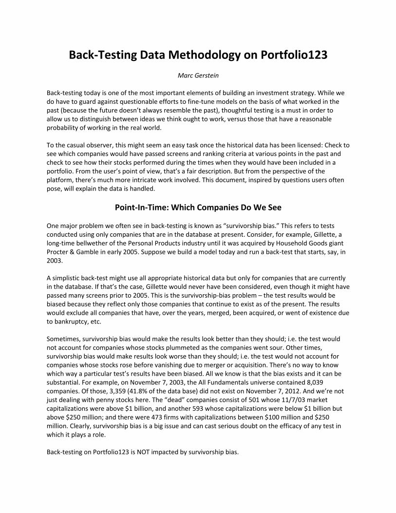
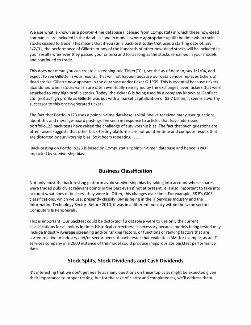
Figure 2 is a Portfolio123 screen that uses a line-item function to reveal these last three annual shares-outstanding figures and a recent share price as well as share prices dating back approximately one and two year. Figure 3 shows the Results. Figure 2
Figure 3
Notice that the actual number of shares, as shown on Compustat for the two pre-split years, was 147.431 million. Notice, too that the number of shares for those same pre-split periods is shown on Portfolio123 as 294.86, a figure that reflects the 2-for-1 split.
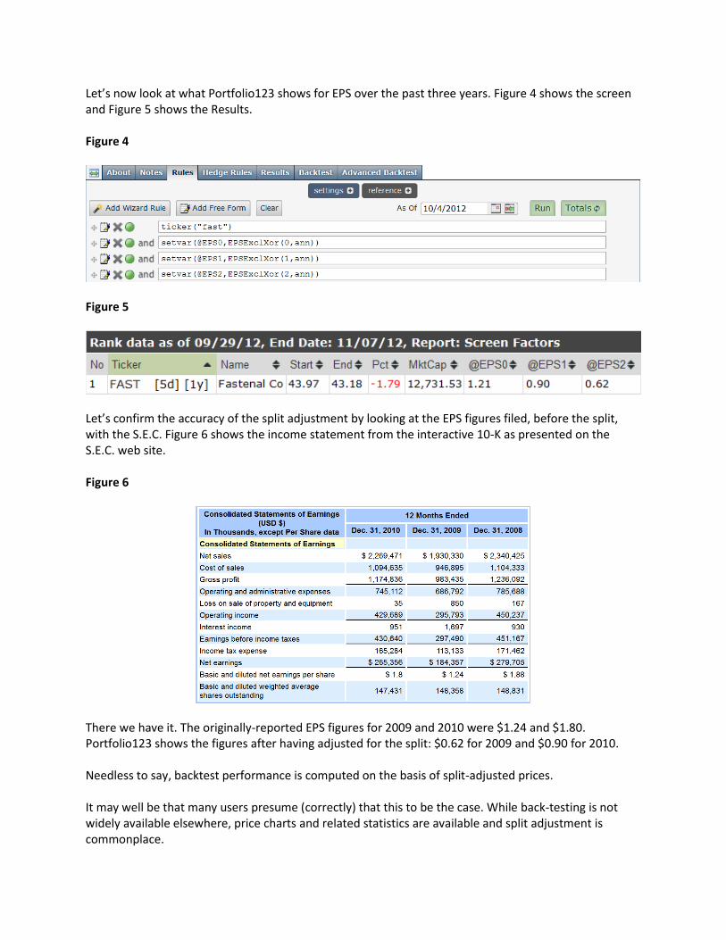
Let’s now look at what Portfolio123 shows for EPS over the past three years. Figure 4 shows the screen and Figure 5 shows the Results. Figure 4
Figure 5
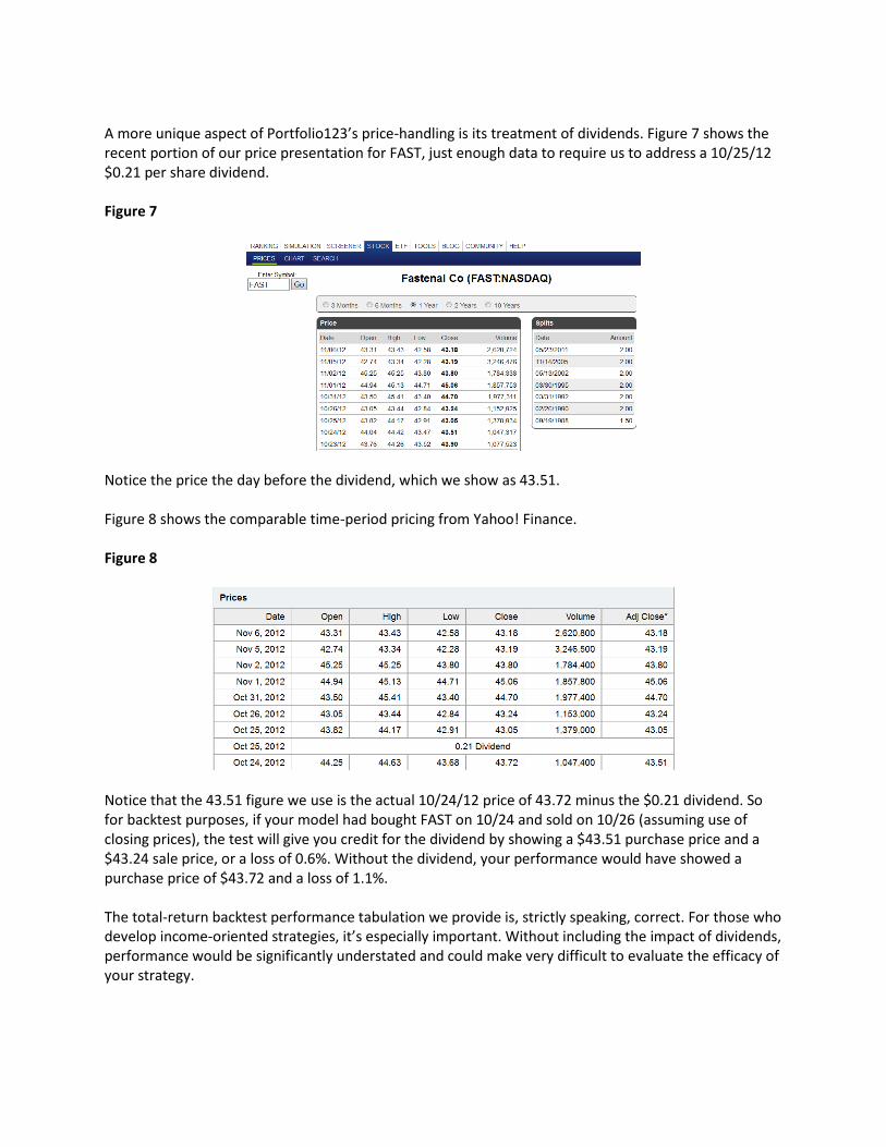
Let’s confirm the accuracy of the split adjustment by looking at the EPS figures filed, before the split, with the S.E.C. Figure 6 shows the income statement from the interactive 10-K as presented on the S.E.C. web site. Figure 6
There we have it. The originally-reported EPS figures for 2009 and 2010 were $1.24 and $1.80. Portfolio123 shows the figures after having adjusted for the split: $0.62 for 2009 and $0.90 for 2010. Needless to say, backtest performance is computed on the basis of split-adjusted prices. It may well be that many users presume (correctly) that this to be the case. While back-testing is not widely available elsewhere, price charts and related statistics are available and split adjustment is commonplace.
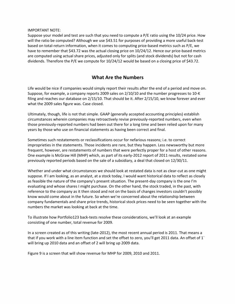
A more unique aspect of Portfolio123’s price-handling is its treatment of dividends. Figure 7 shows the recent portion of our price presentation for FAST, just enough data to require us to address a 10/25/12 $0.21 per share dividend. Figure 7
Notice the price the day before the dividend, which we show as 43.51. Figure 8 shows the comparable time-period pricing from Yahoo! Finance. Figure 8
Notice that the 43.51 figure we use is the actual 10/24/12 price of 43.72 minus the $0.21 dividend. So for backtest purposes, if your model had bought FAST on 10/24 and sold on 10/26 (assuming use of closing prices), the test will give you credit for the dividend by showing a $43.51 purchase price and a $43.24 sale price, or a loss of 0.6%. Without the dividend, your performance would have showed a purchase price of $43.72 and a loss of 1.1%. The total-return backtest performance tabulation we provide is, strictly speaking, correct. For those who develop income-oriented strategies, it’s especially important. Without including the impact of dividends, performance would be significantly understated and could make very difficult to evaluate the efficacy of your strategy.
IMPORTANT NOTE: Suppose your model and test are such that you need to compute a P/E ratio using the 10/24 price. How will the ratio be computed? Although we use $43.51 for purposes of providing a more useful back-test based on total-return information, when it comes to computing price-based metrics such as P/E, we have to remember that $43.72 was the actual closing price on 10/24/12. Hence our price-based metrics are computed using actual share prices, adjusted only for splits (and stock dividends) but not for cash dividends. Therefore the P/E we compute for 10/24/12 would be based on a closing price of $43.72.
What Are the Numbers Life would be nice if companies would simply report their results after the end of a period and move on. Suppose, for example, a company reports 2009 sales on 2/10/10 and the number progresses to 10-K filing and reaches our database on 2/15/10. That should be it. After 2/15/10, we know forever and ever what the 2009 sales figure was. Case closed. Ultimately, though, life is not that simple. GAAP (generally accepted accounting principles) establish circumstances wherein companies may retroactively revise previously-reported numbers, even when those previously-reported numbers had been out there for a long time and been relied upon for many years by those who use on financial statements as having been correct and final. Sometimes such restatements or reclassifications occur for nefarious reasons; i.e. to correct improprieties in the statements. Those incidents are rare, but they happen. Less newsworthy but more frequent, however, are restatements of numbers that were perfectly proper for a host of other reasons. One example is McGraw Hill (MHP) which, as part of its early-2012 report of 2011 results, restated some previously reported periods based on the sale of a subsidiary, a deal that closed on 12/30/11. Whether and under what circumstances we should look at restated data is not as clear-cut as one might suppose. If I am looking, as an analyst, at a stock today, I would want historical data to reflect as closely as feasible the nature of the company’s present situation. The present-day company is the one I’m evaluating and whose shares I might purchase. On the other hand, the stock traded, in the past, with reference to the company as it then stood and not on the basis of changes investors couldn’t possibly know would come about in the future. So when we’re concerned about the relationship between company fundamentals and share price trends, historical stock prices need to be seen together with the numbers the market was looking at back at the time. To illustrate how Portfolio123 back-tests resolve these considerations, we’ll look at an example consisting of one number, total revenue for 2009. In a screen created as of this writing (late-2012), the most recent annual period is 2011. That means a that if you work with a line item function and set the offset to zero, you’ll get 2011 data. An offset of 1` will bring up 2010 data and an offset of 2 will bring up 2009 data. Figure 9 is a screen that will show revenue for MHP for 2009, 2010 and 2011.
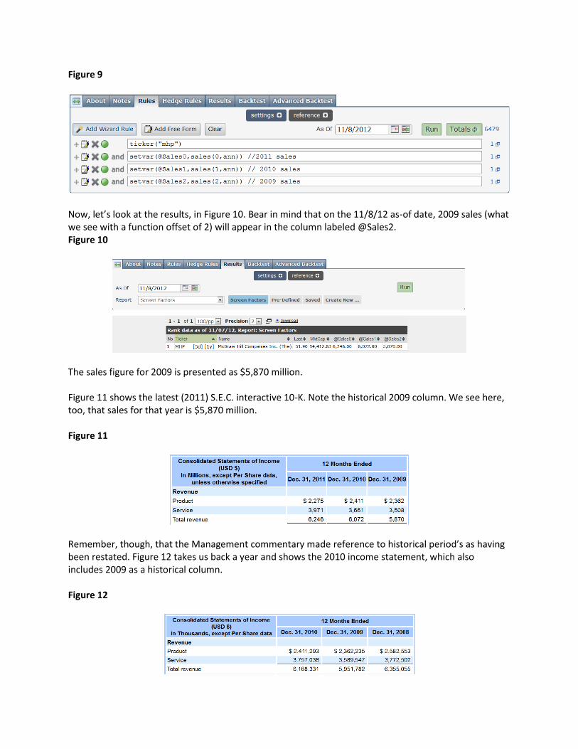
Figure 9
Now, let’s look at the results, in Figure 10. Bear in mind that on the 11/8/12 as-of date, 2009 sales (what we see with a function offset of 2) will appear in the column labeled @Sales2. Figure 10
The sales figure for 2009 is presented as $5,870 million. Figure 11 shows the latest (2011) S.E.C. interactive 10-K. Note the historical 2009 column. We see here, too, that sales for that year is $5,870 million. Figure 11
Remember, though, that the Management commentary made reference to historical period’s as having been restated. Figure 12 takes us back a year and shows the 2010 income statement, which also includes 2009 as a historical column. Figure 12
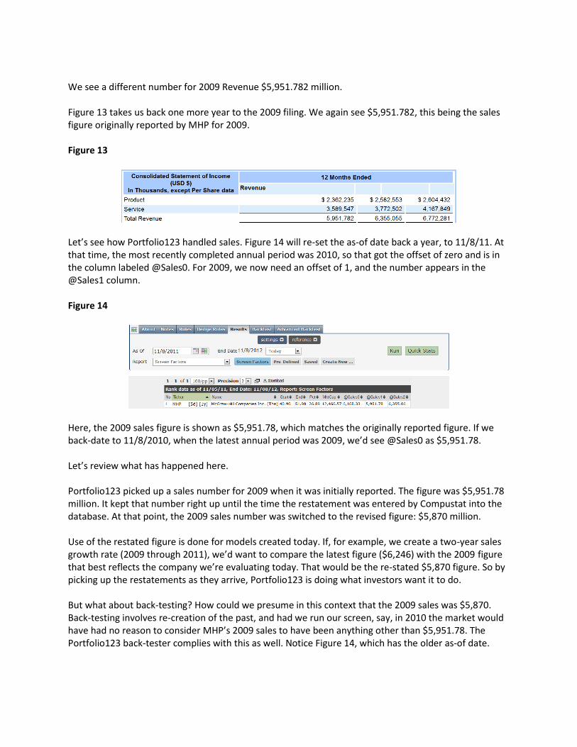
We see a different number for 2009 Revenue $5,951.782 million. Figure 13 takes us back one more year to the 2009 filing. We again see $5,951.782, this being the sales figure originally reported by MHP for 2009. Figure 13
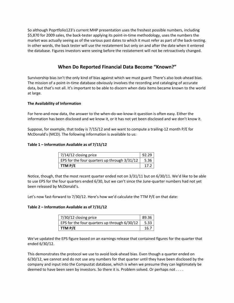
Let’s see how Portfolio123 handled sales. Figure 14 will re-set the as-of date back a year, to 11/8/11. At that time, the most recently completed annual period was 2010, so that got the offset of zero and is in the column labeled @Sales0. For 2009, we now need an offset of 1, and the number appears in the @Sales1 column. Figure 14
Here, the 2009 sales figure is shown as $5,951.78, which matches the originally reported figure. If we back-date to 11/8/2010, when the latest annual period was 2009, we’d see @Sales0 as $5,951.78. Let’s review what has happened here. Portfolio123 picked up a sales number for 2009 when it was initially reported. The figure was $5,951.78 million. It kept that number right up until the time the restatement was entered by Compustat into the database. At that point, the 2009 sales number was switched to the revised figure: $5,870 million. Use of the restated figure is done for models created today. If, for example, we create a two-year sales growth rate (2009 through 2011), we’d want to compare the latest figure ($6,246) with the 2009 figure that best reflects the company we’re evaluating today. That would be the re-stated $5,870 figure. So by picking up the restatements as they arrive, Portfolio123 is doing what investors want it to do. But what about back-testing? How could we presume in this context that the 2009 sales was $5,870. Back-testing involves re-creation of the past, and had we run our screen, say, in 2010 the market would have had no reason to consider MHP’s 2009 sales to have been anything other than $5,951.78. The Portfolio123 back-tester complies with this as well. Notice Figure 14, which has the older as-of date.
So although Poprtfolio123’s current MHP presentation uses the freshest possible numbers, including $5,870 for 2009 sales, the back-tester applying its point-in-time methodology, uses the numbers the market was actually seeing as of the various past dates to which it must refer as part of the back-testing. In other words, the back tester will use the restatement but only on and after the date when it entered the database. Figures investors were seeing before the restatement will not be retroactively changed.
When Do Reported Financial Data Become “Known?” Survivorship bias isn’t the only kind of bias against which we must guard: There’s also look-ahead bias. The mission of a point-in-time database obviously involves the recording and cataloging of accurate data, but that’s not all. It’s important to be able to discern when data items became known to the world at large. The Availability of Information For here-and-now data, the answer to the when-do-we-know-it question is often easy. Either the information has been disclosed and we know it, or it has not yet been disclosed and we don’t know it. Suppose, for example, that today is 7/15/12 and we want to compute a trailing-12 month P/E for McDonald’s (MCD). The following information is available to us: Table 1 – Information Available as of 7/15/12
7/14/12 closing price 92.29
EPS for the four quarters up through 3/31/12 5.36
TTM P/E 17.2
Notice, though, that the most recent quarter ended not on 3/31/11 but on 6/30/11. We’d like to be able to use EPS for the four quarters ended 6/30, but we can’t since the June-quarter numbers had not yet been released by McDonald’s. Let’s now fast-forward to 7/30/12. Here’s how we’d calculate the TTM P/E on that date: Table 2 – Information Available as of 7/31/12
7/30/12 closing price 89.36
EPS for the four quarters up through 6/30/12 5.33
TTM P/E 16.7
We’ve updated the EPS figure based on an earnings release that contained figures for the quarter that ended 6/30/12. This demonstrates the protocol we use to avoid look-ahead bias. Even though a quarter ended on 6/30/12, we cannot and do not use any numbers for that quarter until they have been disclosed by the company and input into the Compustat database, which is when we presume they can legitimately be deemed to have been seen by investors. So there it is. Problem solved. Or perhaps not . . . .
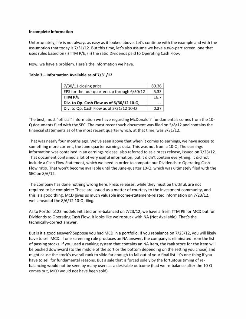
Incomplete Information Unfortunately, life is not always as easy as it looked above. Let’s continue with the example and with the assumption that today is 7/31/12. But this time, let’s also assume we have a two-part screen, one that uses rules based on (i) TTM P/E, (ii) the ratio Dividends paid to Operating Cash Flow. Now, we have a problem. Here’s the information we have. Table 3 – Information Available as of 7/31/12
7/30/11 closing price 89.36
EPS for the four quarters up through 6/30/12 5.33
TTM P/E 16.7
Div. to Op. Cash Flow as of 6/30/12 10-Q - -
Div. to Op. Cash Flow as of 3/31/12 10-Q 0.37
The best, most “official” information we have regarding McDonald’s’ fundamentals comes from the 10-Q documents filed with the SEC. The most recent such document was filed on 5/8/12 and contains the financial statements as of the most recent quarter which, at that time, was 3/31/12. That was nearly four months ago. We’ve seen above that when it comes to earnings, we have access to something more current, the June quarter earnings data. This was not from a 10-Q. The earnings information was contained in an earnings release, also referred to as a press release, issued on 7/23/12. That document contained a lot of very useful information, but it didn’t contain everything. It did not include a Cash Flow Statement, which we need in order to compute our Dividends to Operating Cash Flow ratio. That won’t become available until the June-quarter 10-Q, which was ultimately filed with the SEC on 8/6/12. The company has done nothing wrong here. Press releases, while they must be truthful, are not required to be complete: These are issued as a matter of courtesy to the investment community, and this is a good thing. MCD gives us much valuable income-statement-related information on 7/23/12, well ahead of the 8/6/12 10-Q filing. As to Portfolio123 models initiated or re-balanced on 7/23/12, we have a fresh TTM PE for MCD but for Dividends to Operating Cash Flow, it looks like we’re stuck with NA (Not Available). That’s the technically-correct answer. But is it a good answer? Suppose you had MCD in a portfolio. If you rebalance on 7/23/12, you will likely have to sell MCD. If one screening rule produces an NA answer, the company is eliminated from the list of passing stocks. If you used a ranking system that contains an NA item, the rank score for the item will be pushed downward (to the middle of the sort or the bottom depending on the setting you chose) and might cause the stock’s overall rank to slide far enough to fall out of your final list. It’s one thing if you have to sell for fundamental reasons. But a sale that is forced solely by the fortuitous timing of re-balancing would not be seen by many users as a desirable outcome (had we re-balance after the 10-Q comes out, MCD would not have been sold).
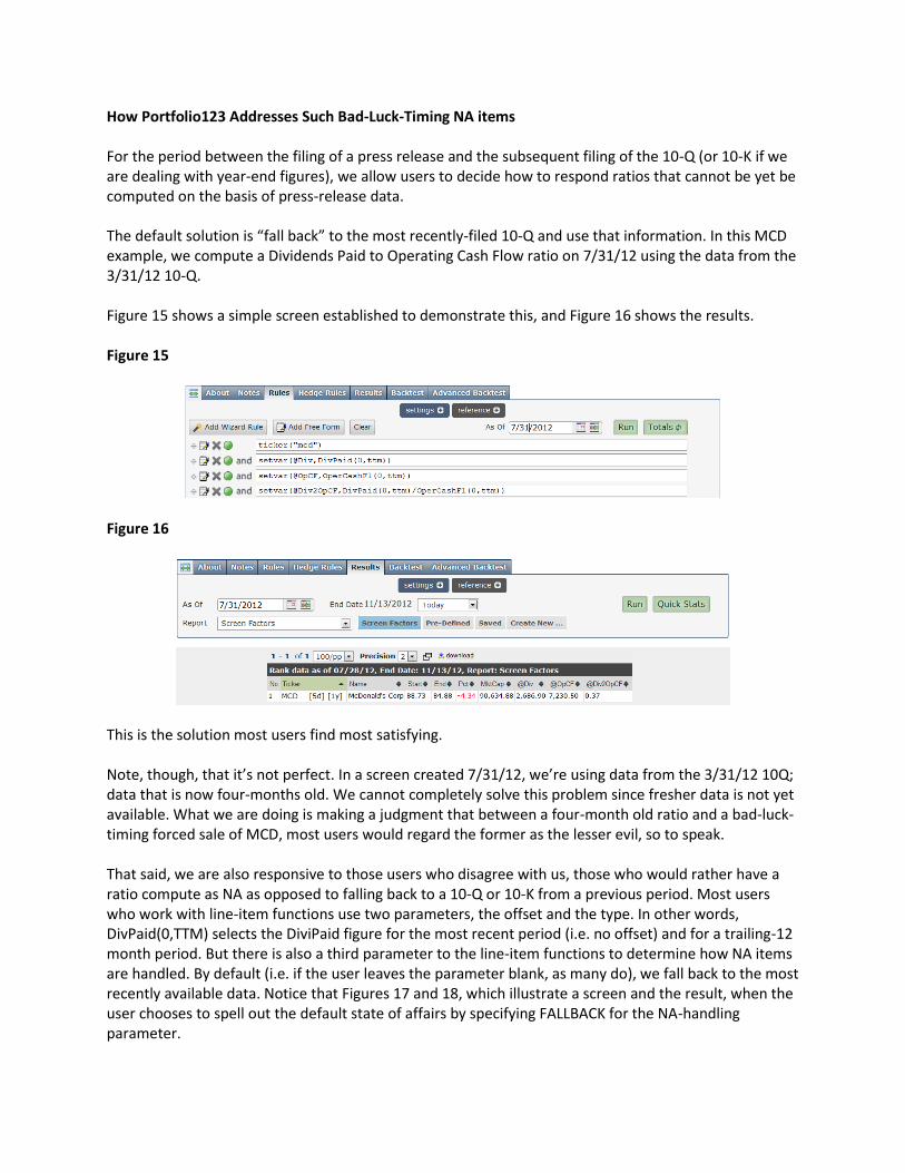
How Portfolio123 Addresses Such Bad-Luck-Timing NA items For the period between the filing of a press release and the subsequent filing of the 10-Q (or 10-K if we are dealing with year-end figures), we allow users to decide how to respond ratios that cannot be yet be computed on the basis of press-release data. The default solution is “fall back” to the most recently-filed 10-Q and use that information. In this MCD example, we compute a Dividends Paid to Operating Cash Flow ratio on 7/31/12 using the data from the 3/31/12 10-Q. Figure 15 shows a simple screen established to demonstrate this, and Figure 16 shows the results. Figure 15
Figure 16
This is the solution most users find most satisfying. Note, though, that it’s not perfect. In a screen created 7/31/12, we’re using data from the 3/31/12 10Q; data that is now four-months old. We cannot completely solve this problem since fresher data is not yet available. What we are doing is making a judgment that between a four-month old ratio and a bad-luck-timing forced sale of MCD, most users would regard the former as the lesser evil, so to speak. That said, we are also responsive to those users who disagree with us, those who would rather have a ratio compute as NA as opposed to falling back to a 10-Q or 10-K from a previous period. Most users who work with line-item functions use two parameters, the offset and the type. In other words, DivPaid(0,TTM) selects the DiviPaid figure for the most recent period (i.e. no offset) and for a trailing-12 month period. But there is also a third parameter to the line-item functions to determine how NA items are handled. By default (i.e. if the user leaves the parameter blank, as many do), we fall back to the most recently available data. Notice that Figures 17 and 18, which illustrate a screen and the result, when the user chooses to spell out the default state of affairs by specifying FALLBACK for the NA-handling parameter.
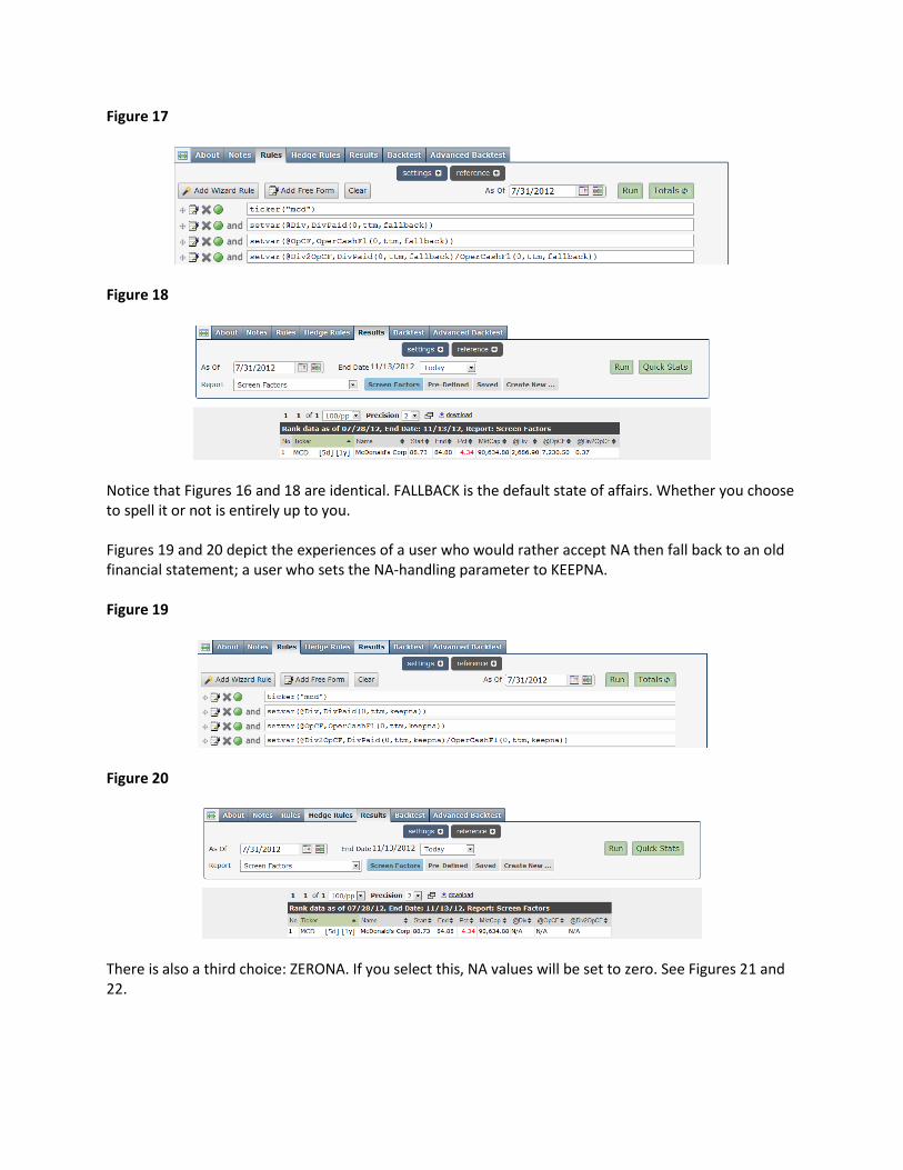
Figure 17
Figure 18
Notice that Figures 16 and 18 are identical. FALLBACK is the default state of affairs. Whether you choose to spell it or not is entirely up to you. Figures 19 and 20 depict the experiences of a user who would rather accept NA then fall back to an old financial statement; a user who sets the NA-handling parameter to KEEPNA. Figure 19
Figure 20
There is also a third choice: ZERONA. If you select this, NA values will be set to zero. See Figures 21 and 22.
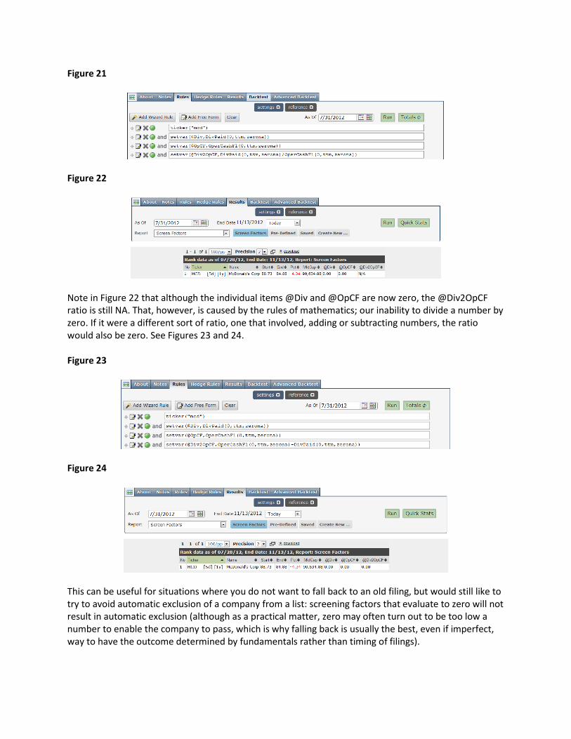
Figure 21
Figure 22
Note in Figure 22 that although the individual items @Div and @OpCF are now zero, the @Div2OpCF ratio is still NA. That, however, is caused by the rules of mathematics; our inability to divide a number by zero. If it were a different sort of ratio, one that involved, adding or subtracting numbers, the ratio would also be zero. See Figures 23 and 24. Figure 23
Figure 24
This can be useful for situations where you do not want to fall back to an old filing, but would still like to try to avoid automatic exclusion of a company from a list: screening factors that evaluate to zero will not result in automatic exclusion (although as a practical matter, zero may often turn out to be too low a number to enable the company to pass, which is why falling back is usually the best, even if imperfect, way to have the outcome determined by fundamentals rather than timing of filings).
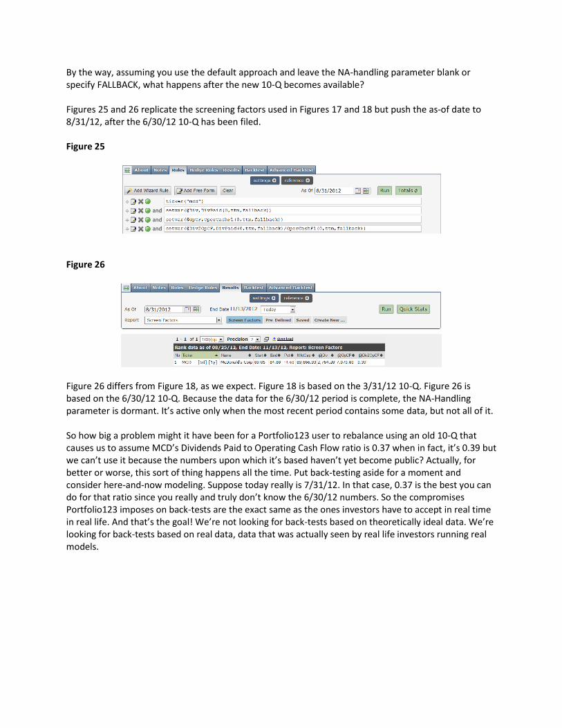
By the way, assuming you use the default approach and leave the NA-handling parameter blank or specify FALLBACK, what happens after the new 10-Q becomes available? Figures 25 and 26 replicate the screening factors used in Figures 17 and 18 but push the as-of date to 8/31/12, after the 6/30/12 10-Q has been filed. Figure 25
Figure 26
Figure 26 differs from Figure 18, as we expect. Figure 18 is based on the 3/31/12 10-Q. Figure 26 is based on the 6/30/12 10-Q. Because the data for the 6/30/12 period is complete, the NA-Handling parameter is dormant. It’s active only when the most recent period contains some data, but not all of it. So how big a problem might it have been for a Portfolio123 user to rebalance using an old 10-Q that causes us to assume MCD’s Dividends Paid to Operating Cash Flow ratio is 0.37 when in fact, it’s 0.39 but we can’t use it because the numbers upon which it’s based haven’t yet become public? Actually, for better or worse, this sort of thing happens all the time. Put back-testing aside for a moment and consider here-and-now modeling. Suppose today really is 7/31/12. In that case, 0.37 is the best you can do for that ratio since you really and truly don’t know the 6/30/12 numbers. So the compromises Portfolio123 imposes on back-tests are the exact same as the ones investors have to accept in real time in real life. And that’s the goal! We’re not looking for back-tests based on theoretically ideal data. We’re looking for back-tests based on real data, data that was actually seen by real life investors running real models.