B02 – Guided Interpretation #2 - KAPPA - Petroleum ...€¦ · Emeraude v2.60 – Doc v2.60.01 - © KAPPA 1988-2010 Guided ... ‘Add’ Manual addition of user ... © KAPPA 1988-2010

Emeraude v2.60 – Doc v2.60.01 - © KAPPA 1988-2010 Guided Interpretation #2 • B02 - 1/22

15BB02 – Guided Interpretation #2

This chapter assumes that you have followed the first guided interpretation and are familiar

with the basic facilities of Emeraude. This second example is for oil-water flow in a deviated

well. Both shut-in and production surveys are available.

B02.1 0B• Starting the session and loading the General Well Data

Start Emeraude and create a new file. In the ‘Units’ tab select ‘Oil Field’.

Go the ‘Document’ control panel and click on ‘Load Well Data’.

Click on ‘Add’.

In the Examples sub-directory of the Emeraude installation select the file B02oh.lis.

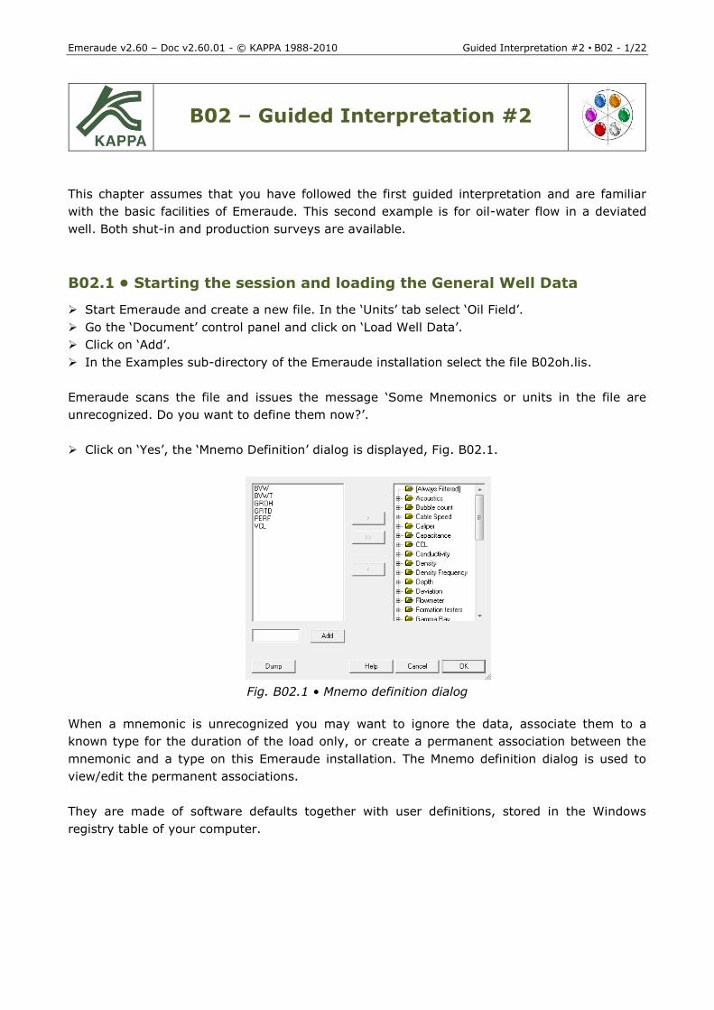
Emeraude scans the file and issues the message ‘Some Mnemonics or units in the file are

unrecognized. Do you want to define them now?’.

Click on ‘Yes’, the ‘Mnemo Definition’ dialog is displayed, Fig. B02.1.

Fig. B02.1 • Mnemo definition dialog

When a mnemonic is unrecognized you may want to ignore the data, associate them to a

known type for the duration of the load only, or create a permanent association between the

mnemonic and a type on this Emeraude installation. The Mnemo definition dialog is used to

view/edit the permanent associations.

They are made of software defaults together with user definitions, stored in the Windows

registry table of your computer.


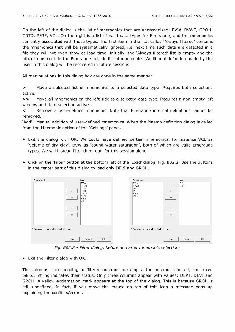
On the left of the dialog is the list of mnemonics that are unrecognized: BVW, BVWT, GROH,

GRTD, PERF, VCL. On the right is a list of valid data types for Emeraude, and the mnemonics

currently associated with those types. The first item in the list, called ‘Always filtered’ contains

the mnemonics that will be systematically ignored, i.e. next time such data are detected in a

file they will not even show at load time. Initially, the ‘Always filtered’ list is empty and the

other items contain the Emeraude built-in list of mnemonics. Additional definition made by the

user in this dialog will be recovered in future sessions.

All manipulations in this dialog box are done in the same manner:

> Move a selected list of mnemonics to a selected data type. Requires both selections

active.

>> Move all mnemonics on the left side to a selected data type. Requires a non-empty left

window and right selection active.

< Remove a user-defined mnemonic. Note that Emeraude internal definitions cannot be

removed.

‘Add’ Manual addition of user-defined mnemonics. When the Mnemo definition dialog is called

from the Mnemonic option of the ‘Settings’ panel.

Exit the dialog with OK. We could have defined certain mnemonics, for instance VCL as

‘Volume of dry clay’, BVW as ‘bound water saturation’, both of which are valid Emeraude

types. We will instead filter them out, for this session alone.

Click on the ‘Filter’ button at the bottom left of the ‘Load’ dialog, Fig. B02.2. Use the buttons

in the center part of this dialog to load only DEVI and GROH.

Fig. B02.2 • Filter dialog, before and after mnemonic selections

Exit the Filter dialog with OK.

The columns corresponding to filtered mnemos are empty, the mnemo is in red, and a red

‘Skip…’ string indicates their status. Only three columns appear with values: DEPT, DEVI and

GROH. A yellow exclamation mark appears at the top of the dialog. This is because GROH is

still undefined. In fact, if you move the mouse on top of this icon a message pops up

explaining the conflicts/errors.


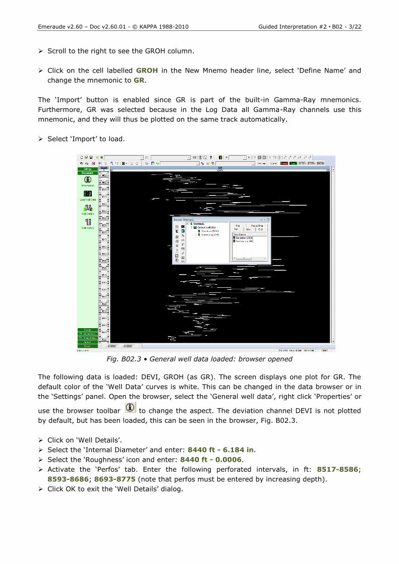
Scroll to the right to see the GROH column.

Click on the cell labelled GROH in the New Mnemo header line, select ‘Define Name’ and

change the mnemonic to GR.

The ‘Import’ button is enabled since GR is part of the built-in Gamma-Ray mnemonics.

Furthermore, GR was selected because in the Log Data all Gamma-Ray channels use this

mnemonic, and they will thus be plotted on the same track automatically.

Select ‘Import’ to load.

Fig. B02.3 • General well data loaded: browser opened

The following data is loaded: DEVI, GROH (as GR). The screen displays one plot for GR. The

default color of the ‘Well Data’ curves is white. This can be changed in the data browser or in

the ‘Settings’ panel. Open the browser, select the ‘General well data’, right click ‘Properties’ or

use the browser toolbar to change the aspect. The deviation channel DEVI is not plotted

by default, but has been loaded, this can be seen in the browser, Fig. B02.3.

Click on ‘Well Details’.

Select the ‘Internal Diameter’ and enter: 8440 ft - 6.184 in.

Select the ‘Roughness’ icon and enter: 8440 ft - 0.0006.

Activate the ‘Perfos’ tab. Enter the following perforated intervals, in ft: 8517-8586;

8593-8686; 8693-8775 (note that perfos must be entered by increasing depth).

Click OK to exit the ‘Well Details’ dialog.


B02.2 1B• Loading the log data

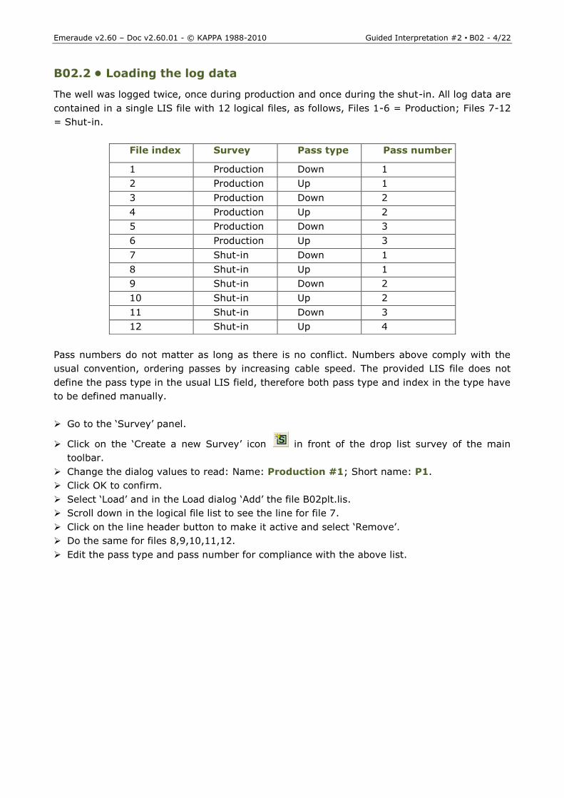
The well was logged twice, once during production and once during the shut-in. All log data are

contained in a single LIS file with 12 logical files, as follows, Files 1-6 = Production; Files 7-12

= Shut-in.

Pass numbers do not matter as long as there is no conflict. Numbers above comply with the

usual convention, ordering passes by increasing cable speed. The provided LIS file does not

define the pass type in the usual LIS field, therefore both pass type and index in the type have

to be defined manually.

Go to the ‘Survey’ panel.

Click on the ‘Create a new Survey’ icon in front of the drop list survey of the main

toolbar.

Change the dialog values to read: Name: Production #1; Short name: P1.

Click OK to confirm.

Select ‘Load’ and in the Load dialog ‘Add’ the file B02plt.lis.

Scroll down in the logical file list to see the line for file 7.

Click on the line header button to make it active and select ‘Remove’.

Do the same for files 8,9,10,11,12.

Edit the pass type and pass number for compliance with the above list.

File index Survey Pass type Pass number

1 Production Down 1

2 Production Up 1

3 Production Down 2

4 Production Up 2

5 Production Down 3

6 Production Up 3

7 Shut-in Down 1

8 Shut-in Up 1

9 Shut-in Down 2

10 Shut-in Up 2

11 Shut-in Down 3

12 Shut-in Up 4


Fig. B02.4 • Production logical files: pass type + number edited

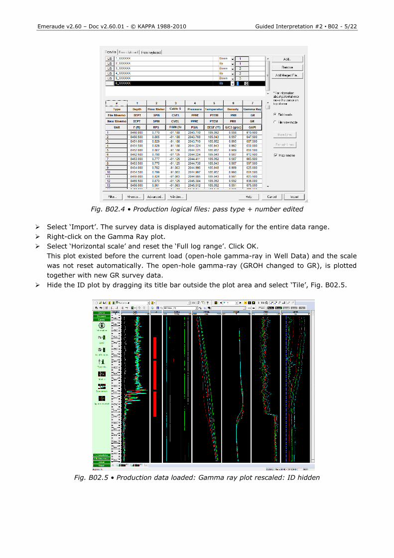
Select ‘Import’. The survey data is displayed automatically for the entire data range.

Right-click on the Gamma Ray plot.

Select ‘Horizontal scale’ and reset the ‘Full log range’. Click OK.

This plot existed before the current load (open-hole gamma-ray in Well Data) and the scale

was not reset automatically. The open-hole gamma-ray (GROH changed to GR), is plotted

together with new GR survey data.

Hide the ID plot by dragging its title bar outside the plot area and select ‘Tile’, Fig. B02.5.

Fig. B02.5 • Production data loaded: Gamma ray plot rescaled: ID hidden


Click on ‘Create a new Survey’ icon in front of the survey drop list of the main toolbar

to create the second survey. By default the name ‘Survey #2’ is proposed.

Edit the dialog values to read:

Name: Shut-in #1

Short name: S1

Hit OK to confirm.

Select ‘Load’ to import the logical files from 7 to 12 from B02plt.lis.

File index Survey Pass type Pass number

7 Shut-in Down 1

8 Shut-in Up 1

9 Shut-in Down 2

10 Shut-in Up 2

11 Shut-in Down 3

12 Shut-in Up 3

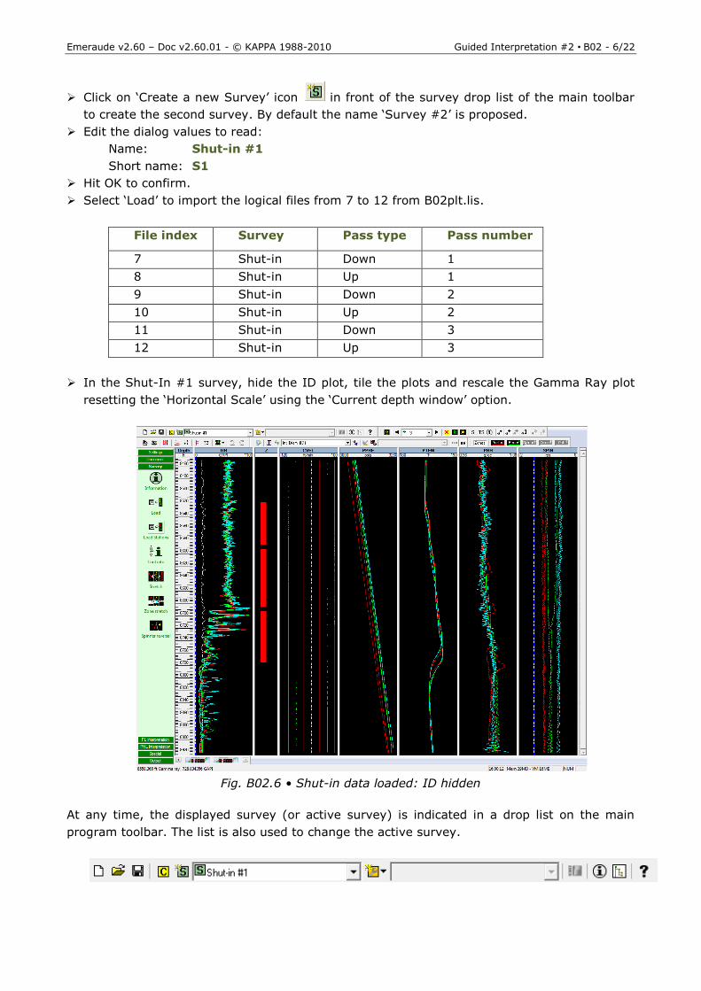
In the Shut-In #1 survey, hide the ID plot, tile the plots and rescale the Gamma Ray plot

resetting the ‘Horizontal Scale’ using the ‘Current depth window’ option.

Fig. B02.6 • Shut-in data loaded: ID hidden

At any time, the displayed survey (or active survey) is indicated in a drop list on the main

program toolbar. The list is also used to change the active survey.


B02.3 2B• Analysis of the Shut-in survey

B02.3.1 5B• Depth match

Make sure that the Shut-in survey is active using the above drop list.

Because of radioactive scale the Shut-in gamma ray does not compare well with the open-hole

curve (Well data). Some correlation is seen below 8770 onwards and can be used for the depth

match. The process of depth matching was covered in Guided interpretation #1.

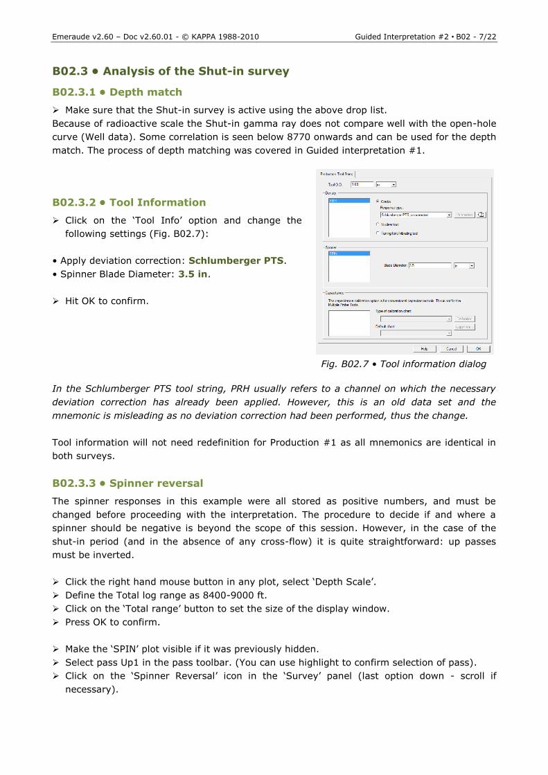
B02.3.2 6B• Tool Information

Click on the ‘Tool Info’ option and change the

following settings (Fig. B02.7):

• Apply deviation correction: Schlumberger PTS.

• Spinner Blade Diameter: 3.5 in.

Hit OK to confirm.

Fig. B02.7 • Tool information dialog

In the Schlumberger PTS tool string, PRH usually refers to a channel on which the necessary

deviation correction has already been applied. However, this is an old data set and the

mnemonic is misleading as no deviation correction had been performed, thus the change.

Tool information will not need redefinition for Production #1 as all mnemonics are identical in

both surveys.

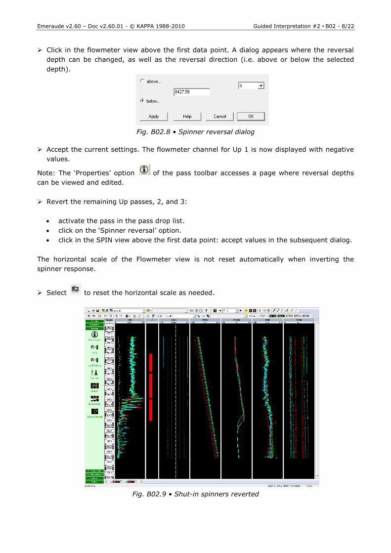
B02.3.3 7B• Spinner reversal

The spinner responses in this example were all stored as positive numbers, and must be

changed before proceeding with the interpretation. The procedure to decide if and where a

spinner should be negative is beyond the scope of this session. However, in the case of the

shut-in period (and in the absence of any cross-flow) it is quite straightforward: up passes

must be inverted.

Click the right hand mouse button in any plot, select ‘Depth Scale’.

Define the Total log range as 8400-9000 ft.

Click on the ‘Total range’ button to set the size of the display window.

Press OK to confirm.

Make the ‘SPIN’ plot visible if it was previously hidden.

Select pass Up1 in the pass toolbar. (You can use highlight to confirm selection of pass).

Click on the ‘Spinner Reversal’ icon in the ‘Survey’ panel (last option down - scroll if

necessary).


Click in the flowmeter view above the first data point. A dialog appears where the reversal

depth can be changed, as well as the reversal direction (i.e. above or below the selected

depth).

Fig. B02.8 • Spinner reversal dialog

Accept the current settings. The flowmeter channel for Up 1 is now displayed with negative

values.

Note: The ‘Properties’ option of the pass toolbar accesses a page where reversal depths

can be viewed and edited.

Revert the remaining Up passes, 2, and 3:

activate the pass in the pass drop list.

click on the ‘Spinner reversal’ option.

click in the SPIN view above the first data point: accept values in the subsequent dialog.

The horizontal scale of the Flowmeter view is not reset automatically when inverting the

spinner response.

Select to reset the horizontal scale as needed.

Fig. B02.9 • Shut-in spinners reverted


B02.3.4 8B• Creating a new interpretation

Move to the ‘PL Interpretation’ panel.

Select the ‘Information’ icon.

This is the first interpretation for the active survey: an interpretation is created automatically,

called Interpretation#1.

Note: To create a new interpretation after one exists, you need to use the ‘Create a new

Interpretation’ icon in front of the interpretation drop list of the main toolbar.

Leave this name unchanged and validate with OK.

In the ‘Reference channels’ tab of the ‘Interpretation Settings’ dialog, Define the reference

Temperature as that of Down#1.

Define the reference Pressure as an average of All pressure passes during the Shut-in.

Define the reference Density as an average of All the density passes except Up3 and

Down3.

Press OK to confirm.

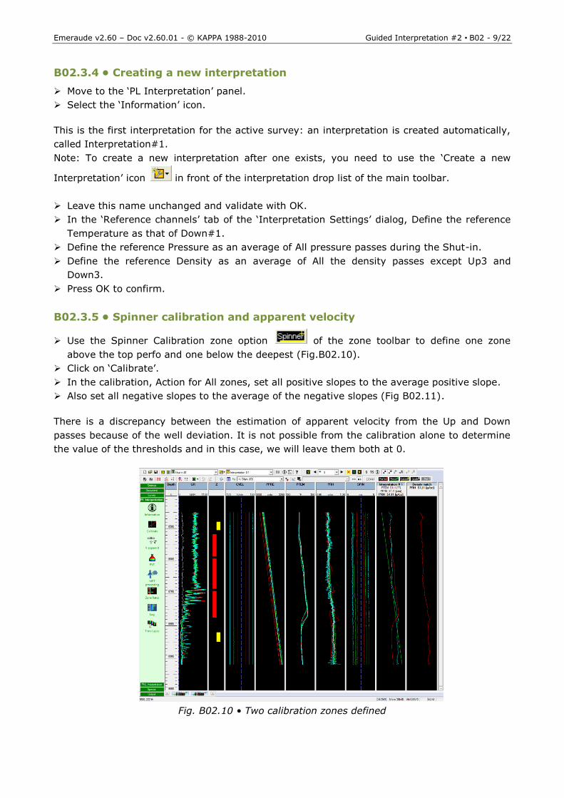
B02.3.5 9B• Spinner calibration and apparent velocity

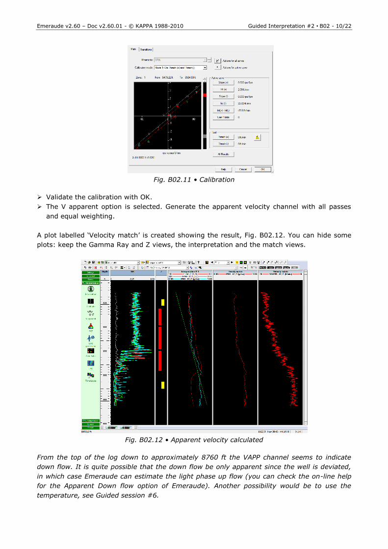
Use the Spinner Calibration zone option of the zone toolbar to define one zone

above the top perfo and one below the deepest (Fig.B02.10).

Click on ‘Calibrate’.

In the calibration, Action for All zones, set all positive slopes to the average positive slope.

Also set all negative slopes to the average of the negative slopes (Fig B02.11).

There is a discrepancy between the estimation of apparent velocity from the Up and Down

passes because of the well deviation. It is not possible from the calibration alone to determine

the value of the thresholds and in this case, we will leave them both at 0.

Fig. B02.10 • Two calibration zones defined


Fig. B02.11 • Calibration

Validate the calibration with OK.

The V apparent option is selected. Generate the apparent velocity channel with all passes

and equal weighting.

A plot labelled ‘Velocity match’ is created showing the result, Fig. B02.12. You can hide some

plots: keep the Gamma Ray and Z views, the interpretation and the match views.

Fig. B02.12 • Apparent velocity calculated

From the top of the log down to approximately 8760 ft the VAPP channel seems to indicate

down flow. It is quite possible that the down flow be only apparent since the well is deviated,

in which case Emeraude can estimate the light phase up flow (you can check the on-line help

for the Apparent Down flow option of Emeraude). Another possibility would be to use the

temperature, see Guided session #6.


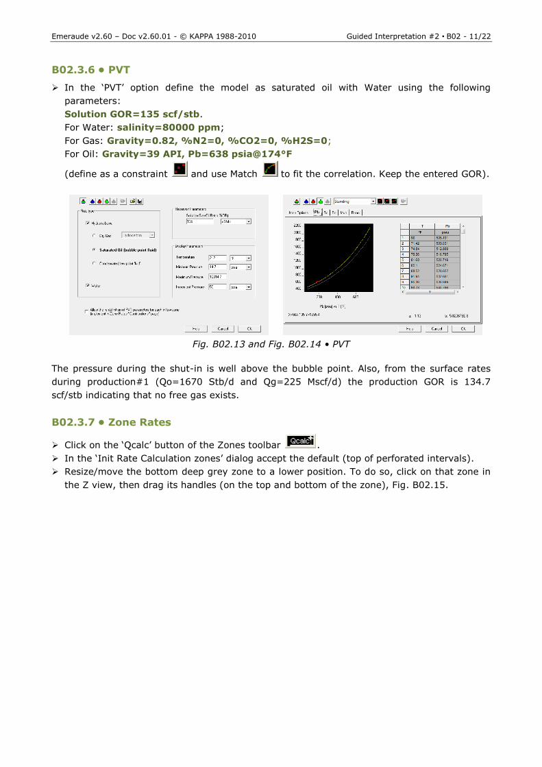
B02.3.6 10B• PVT

In the ‘PVT’ option define the model as saturated oil with Water using the following

parameters:

Solution GOR=135 scf/stb.

For Water: salinity=80000 ppm;

For Gas: Gravity=0.82, %N2=0, %CO2=0, %H2S=0;

For Oil: Gravity=39 API, Pb=638 psia@174°F

(define as a constraint and use Match to fit the correlation. Keep the entered GOR).

Fig. B02.13 and Fig. B02.14 • PVT

The pressure during the shut-in is well above the bubble point. Also, from the surface rates

during production#1 (Qo=1670 Stb/d and Qg=225 Mscf/d) the production GOR is 134.7

scf/stb indicating that no free gas exists.

B02.3.7 11B• Zone Rates

Click on the ‘Qcalc’ button of the Zones toolbar .

In the ‘Init Rate Calculation zones’ dialog accept the default (top of perforated intervals).

Resize/move the bottom deep grey zone to a lower position. To do so, click on that zone in

the Z view, then drag its handles (on the top and bottom of the zone), Fig. B02.15.


Fig. B02.15 • Bottom calculation zone moved down and extended

Select ‘Zone Rates’.

The ‘Init’ page is displayed and a flow model and correlation must be defined. There are two

possible choices with the selected PVT model: Liquid-Gas or Water-Hydrocarbons (L). The

second model is the default as we only have a density measurement. Furthermore, we know

from the saturation pressure and producing GOR that no gas is present during the build-up.

Accept the default model and correlation, and click on the ‘Rate Calculation’ tab.

The main objective of analyzing this shut-in data is to check the density tool reading in a

known fluid type by comparing measured density with predicted values. The density tool

(except for a nuclear tool) does not output the straight density value, but some function of

it; therefore we cannot simply compare PVT predicted densities and tool readings. The zone

rate dialog gives the option to see predicted tool response in 100% oil or 100% water. You

can do this as follows:

Make the bottom zone active, by clicking on the zone in the schematic to the left of the plot,

or use the small arrows above that schematic to move to the required zone.

If Qo is not 0, click on Edit and set it to 0 (Qg is disabled with this particular model

as p > pb).

Set the page to ‘Plot’ mode.

Zoom in (with a right-click on the plot) as shown on the figure below:


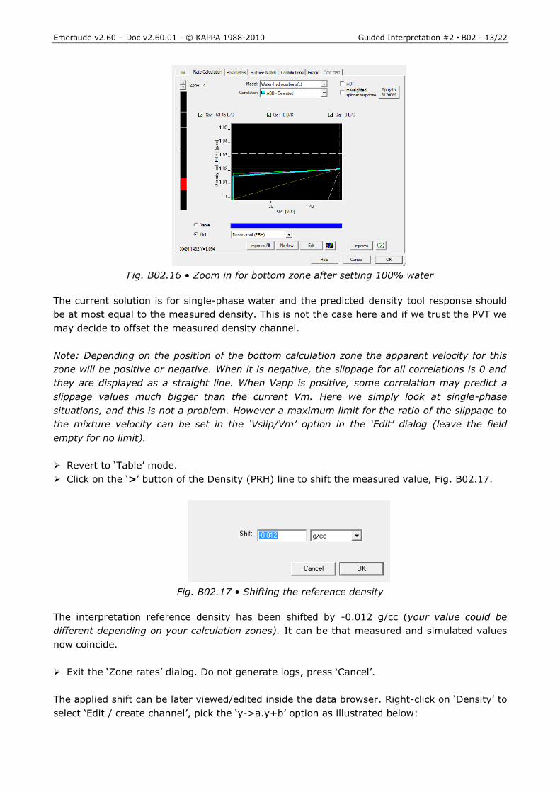
Fig. B02.16 • Zoom in for bottom zone after setting 100% water

The current solution is for single-phase water and the predicted density tool response should

be at most equal to the measured density. This is not the case here and if we trust the PVT we

may decide to offset the measured density channel.

Note: Depending on the position of the bottom calculation zone the apparent velocity for this

zone will be positive or negative. When it is negative, the slippage for all correlations is 0 and

they are displayed as a straight line. When Vapp is positive, some correlation may predict a

slippage values much bigger than the current Vm. Here we simply look at single-phase

situations, and this is not a problem. However a maximum limit for the ratio of the slippage to

the mixture velocity can be set in the ‘Vslip/Vm’ option in the ‘Edit’ dialog (leave the field

empty for no limit).

Revert to ‘Table’ mode.

Click on the ‘>’ button of the Density (PRH) line to shift the measured value, Fig. B02.17.

Fig. B02.17 • Shifting the reference density

The interpretation reference density has been shifted by -0.012 g/cc (your value could be

different depending on your calculation zones). It can be that measured and simulated values

now coincide.

Exit the ‘Zone rates’ dialog. Do not generate logs, press ‘Cancel’.

The applied shift can be later viewed/edited inside the data browser. Right-click on ‘Density’ to

select ‘Edit / create channel’, pick the ‘y->a.y+b’ option as illustrated below:


Fig. B02.18 • Using the browser to view/edit the shift

B02.4 3B• Analysis of the Production survey

B02.4.1 12B• Creating the interpretation

Make Production #1 the active survey using the survey selection drop list in the main

toolbar.

Select the ‘Interpretation’ panel and click on the ‘Information’ icon. Interpretation #1 is

created automatically.

Access is provided to existing interpretations from all surveys. We will use the information

already input for the build-up survey.

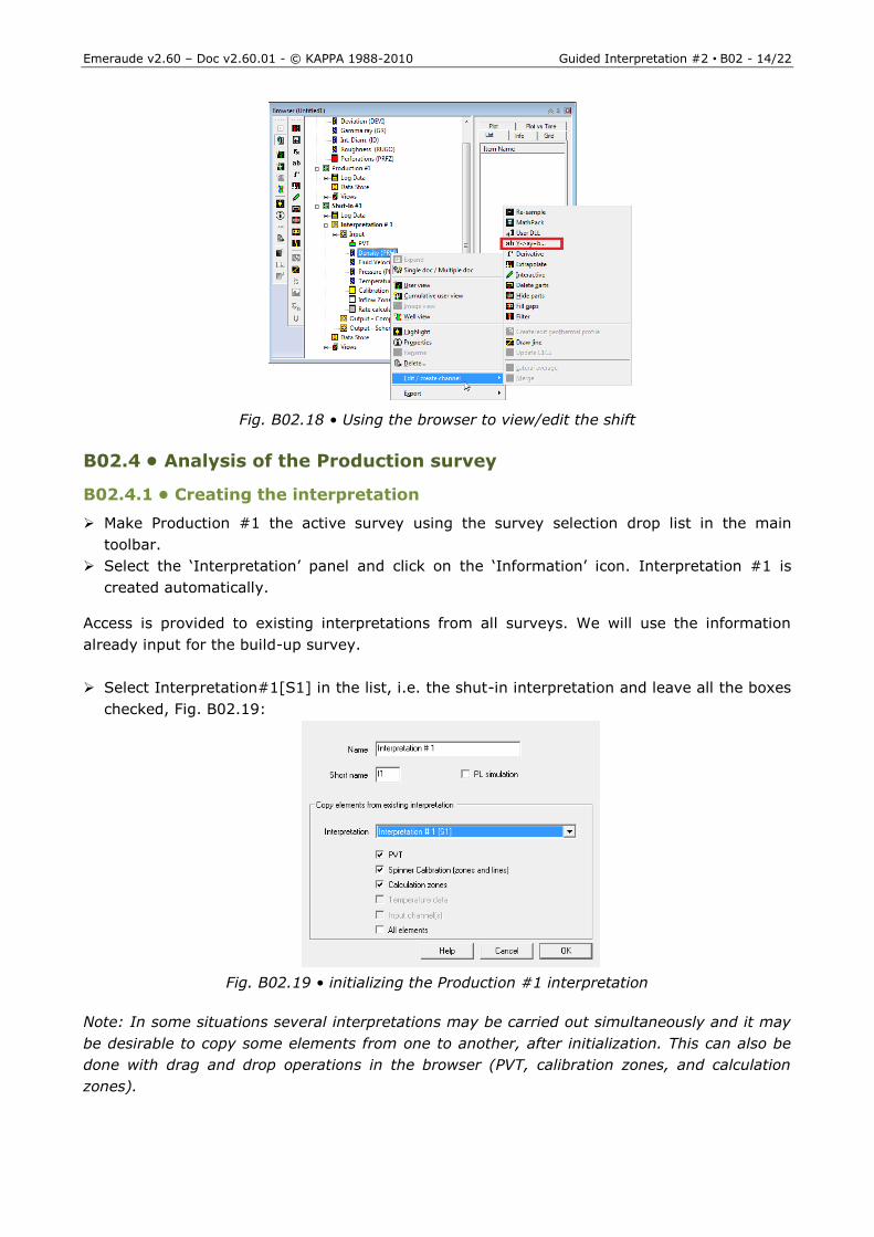
Select Interpretation#1[S1] in the list, i.e. the shut-in interpretation and leave all the boxes

checked, Fig. B02.19:

Fig. B02.19 • initializing the Production #1 interpretation

Note: In some situations several interpretations may be carried out simultaneously and it may

be desirable to copy some elements from one to another, after initialization. This can also be

done with drag and drop operations in the browser (PVT, calibration zones, and calculation

zones).


In the ‘Reference channels’ tab of the ‘Interpretation Settings’ dialog define the temperature

and pressure interpretations as:

Temperature: Down1.

Pressure: average all except Up 1 and Down 1.

Density: average all except Up3 and Down3.

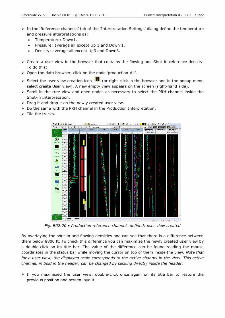
Create a user view in the browser that contains the flowing and Shut-in reference density.

To do this:

Open the data browser, click on the node ‘production #1’.

Select the user view creation icon (or right-click in the browser and in the popup menu

select create User view). A new empty view appears on the screen (right-hand side).

Scroll in the tree view and open nodes as necessary to select the PRH channel inside the

Shut-in Interpretation.

Drag it and drop it on the newly created user view.

Do the same with the PRH channel in the Production Interpretation.

Tile the tracks.

Fig. B02.20 • Production reference channels defined; user view created

By overlaying the shut-in and flowing densities one can see that there is a difference between

them below 8800 ft. To check this difference you can maximize the newly created user view by

a double-click on its title bar. The value of the difference can be found reading the mouse

coordinates in the status bar while moving the cursor on top of them inside the view. Note that

for a user view, the displayed scale corresponds to the active channel in the view. This active

channel, in bold in the header, can be changed by clicking directly inside the header.

If you maximized the user view, double-click once again on its title bar to restore the

previous position and screen layout.


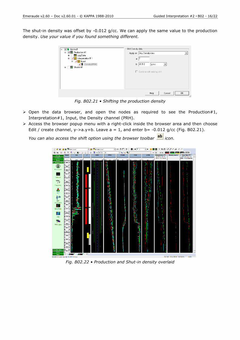
The shut-in density was offset by -0.012 g/cc. We can apply the same value to the production

density. Use your value if you found something different.

Fig. B02.21 • Shifting the production density

Open the data browser, and open the nodes as required to see the Production#1,

Interpretation#1, Input, the Density channel (PRH).

Access the browser popup menu with a right-click inside the browser area and then choose

Edit / create channel, y->a.y+b. Leave a = 1, and enter b= -0.012 g/cc (Fig. B02.21).

You can also access the shift option using the browser toolbar icon.

Fig. B02.22 • Production and Shut-in density overlaid


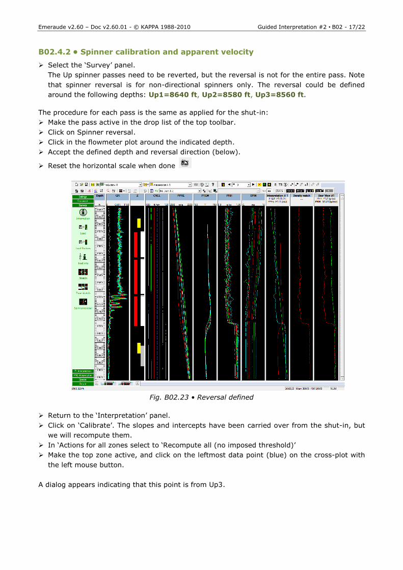
B02.4.2 13B• Spinner calibration and apparent velocity

Select the ‘Survey’ panel.

The Up spinner passes need to be reverted, but the reversal is not for the entire pass. Note

that spinner reversal is for non-directional spinners only. The reversal could be defined

around the following depths: Up1=8640 ft, Up2=8580 ft, Up3=8560 ft.

The procedure for each pass is the same as applied for the shut-in:

Make the pass active in the drop list of the top toolbar.

Click on Spinner reversal.

Click in the flowmeter plot around the indicated depth.

Accept the defined depth and reversal direction (below).

Reset the horizontal scale when done

Fig. B02.23 • Reversal defined

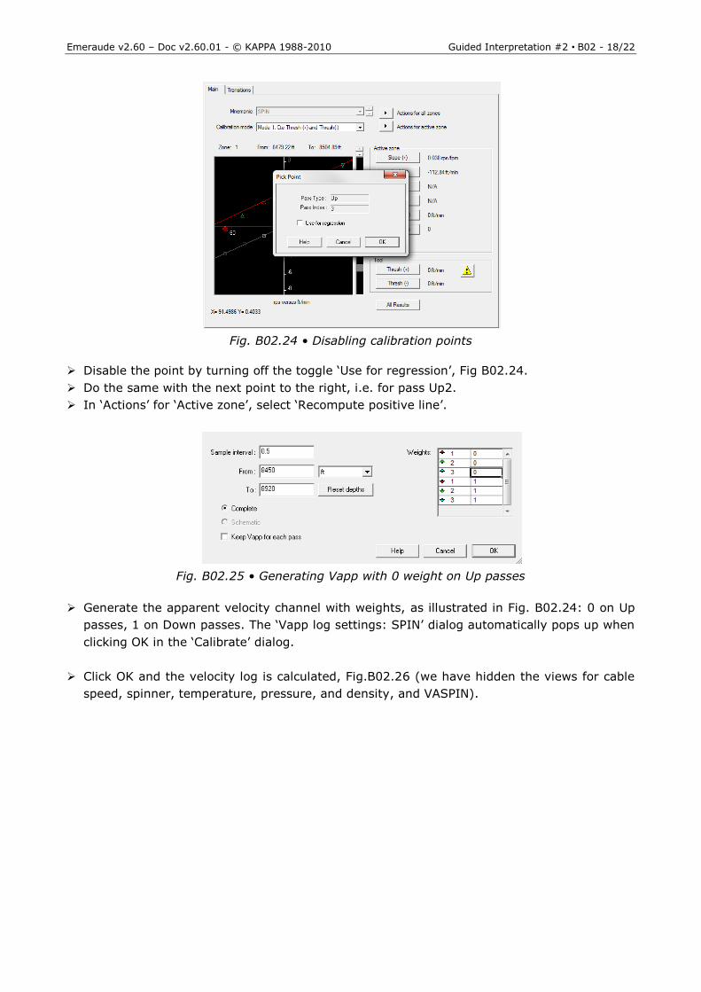
Return to the ‘Interpretation’ panel.

Click on ‘Calibrate’. The slopes and intercepts have been carried over from the shut-in, but

we will recompute them.

In ‘Actions for all zones select to ‘Recompute all (no imposed threshold)’

Make the top zone active, and click on the leftmost data point (blue) on the cross-plot with

the left mouse button.

A dialog appears indicating that this point is from Up3.


Fig. B02.24 • Disabling calibration points

Disable the point by turning off the toggle ‘Use for regression’, Fig B02.24.

Do the same with the next point to the right, i.e. for pass Up2.

In ‘Actions’ for ‘Active zone’, select ‘Recompute positive line’.

Fig. B02.25 • Generating Vapp with 0 weight on Up passes

Generate the apparent velocity channel with weights, as illustrated in Fig. B02.24: 0 on Up

passes, 1 on Down passes. The ‘Vapp log settings: SPIN’ dialog automatically pops up when

clicking OK in the ‘Calibrate’ dialog.

Click OK and the velocity log is calculated, Fig.B02.26 (we have hidden the views for cable

speed, spinner, temperature, pressure, and density, and VASPIN).


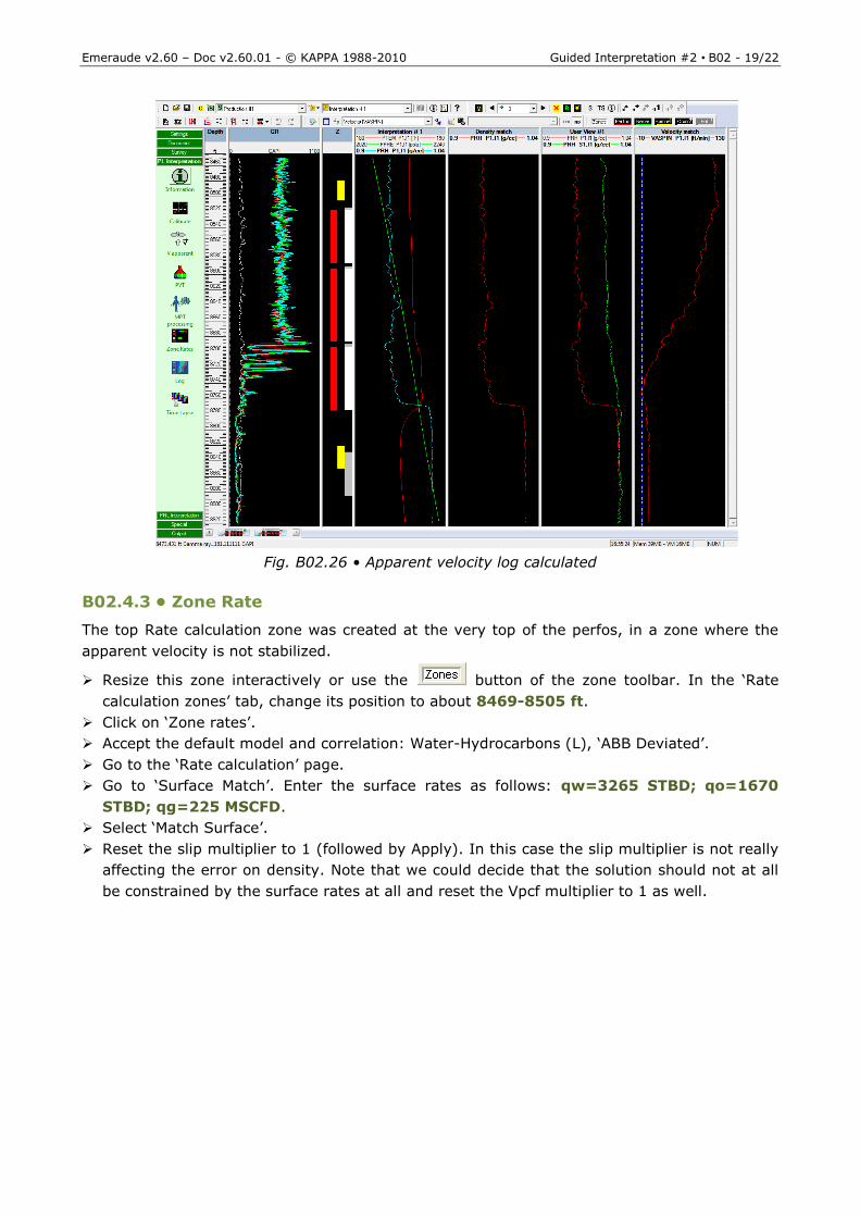
Fig. B02.26 • Apparent velocity log calculated

B02.4.3 14B• Zone Rate

The top Rate calculation zone was created at the very top of the perfos, in a zone where the

apparent velocity is not stabilized.

Resize this zone interactively or use the button of the zone toolbar. In the ‘Rate

calculation zones’ tab, change its position to about 8469-8505 ft.

Click on ‘Zone rates’.

Accept the default model and correlation: Water-Hydrocarbons (L), ‘ABB Deviated’.

Go to the ‘Rate calculation’ page.

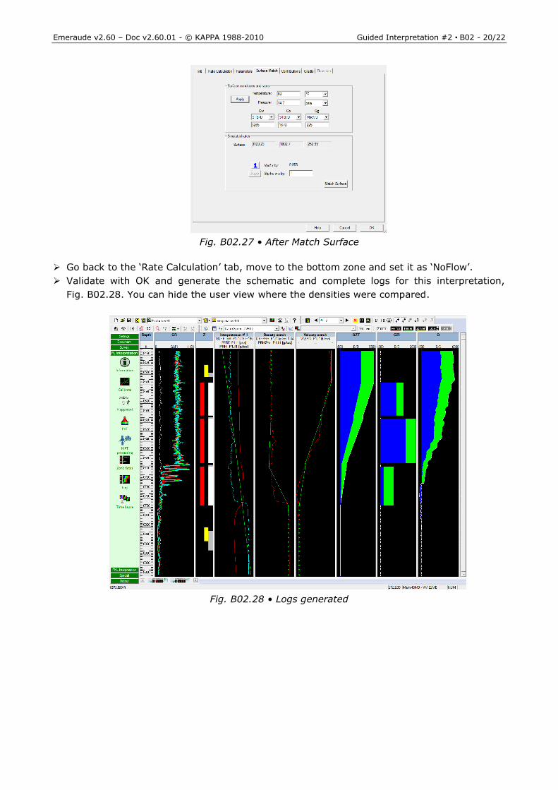
Go to ‘Surface Match’. Enter the surface rates as follows: qw=3265 STBD; qo=1670

STBD; qg=225 MSCFD.

Select ‘Match Surface’.

Reset the slip multiplier to 1 (followed by Apply). In this case the slip multiplier is not really

affecting the error on density. Note that we could decide that the solution should not at all

be constrained by the surface rates at all and reset the Vpcf multiplier to 1 as well.


Fig. B02.27 • After Match Surface

Go back to the ‘Rate Calculation’ tab, move to the bottom zone and set it as ‘NoFlow’.

Validate with OK and generate the schematic and complete logs for this interpretation,

Fig. B02.28. You can hide the user view where the densities were compared.

Fig. B02.28 • Logs generated


B02.5 4B• Additional editing features

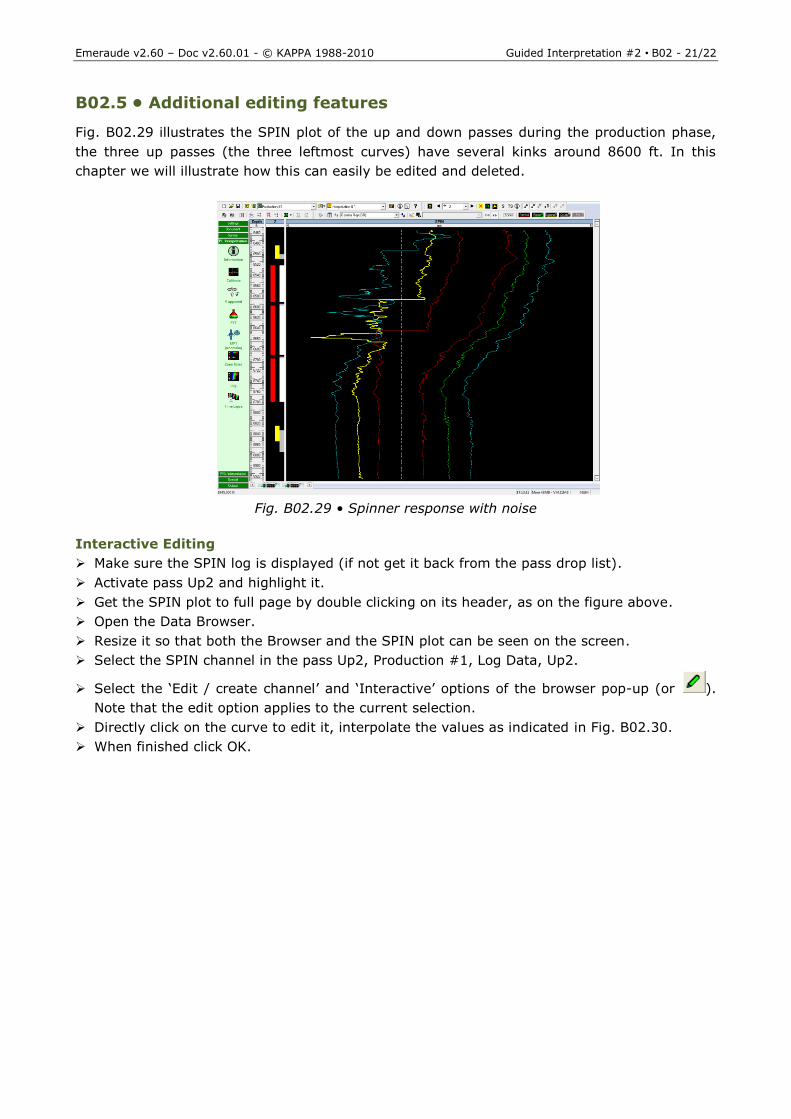
Fig. B02.29 illustrates the SPIN plot of the up and down passes during the production phase,

the three up passes (the three leftmost curves) have several kinks around 8600 ft. In this

chapter we will illustrate how this can easily be edited and deleted.

Fig. B02.29 • Spinner response with noise

Interactive Editing

Make sure the SPIN log is displayed (if not get it back from the pass drop list).

Activate pass Up2 and highlight it.

Get the SPIN plot to full page by double clicking on its header, as on the figure above.

Open the Data Browser.

Resize it so that both the Browser and the SPIN plot can be seen on the screen.

Select the SPIN channel in the pass Up2, Production #1, Log Data, Up2.

Select the ‘Edit / create channel’ and ‘Interactive’ options of the browser pop-up (or ).

Note that the edit option applies to the current selection.

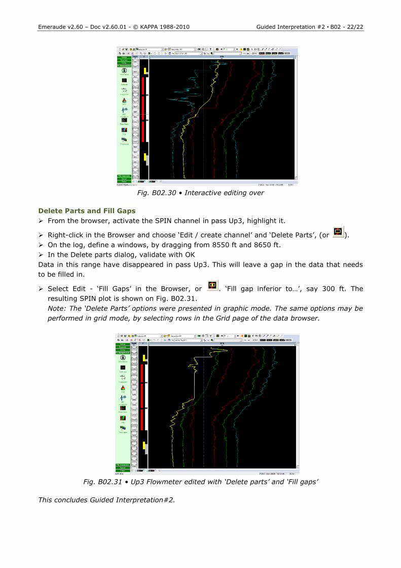
Directly click on the curve to edit it, interpolate the values as indicated in Fig. B02.30.

When finished click OK.


Fig. B02.30 • Interactive editing over

Delete Parts and Fill Gaps

From the browser, activate the SPIN channel in pass Up3, highlight it.

Right-click in the Browser and choose ‘Edit / create channel’ and ‘Delete Parts’, (or ).

On the log, define a windows, by dragging from 8550 ft and 8650 ft.

In the Delete parts dialog, validate with OK

Data in this range have disappeared in pass Up3. This will leave a gap in the data that needs

to be filled in.

Select Edit - ‘Fill Gaps’ in the Browser, or . ‘Fill gap inferior to…’, say 300 ft. The

resulting SPIN plot is shown on Fig. B02.31.

Note: The ‘Delete Parts’ options were presented in graphic mode. The same options may be

performed in grid mode, by selecting rows in the Grid page of the data browser.

Fig. B02.31 • Up3 Flowmeter edited with ‘Delete parts’ and ‘Fill gaps’

This concludes Guided Interpretation#2.

Documents

B02 – Guided Interpretation #2 - KAPPA - Petroleum ...€¦ · Emeraude v2.60 – Doc v2.60.01 - © KAPPA 1988-2010 Guided ... ‘Add’ Manual addition of user ... © KAPPA 1988-2010