B

Topological Network Design:Link Locations

Dr. Greg BernsteinGrotto Networking

www.grotto-networking.com

Outline

• Network Node Types– Access vs. transit

• Expenses: – Capital and Operating

• Link Placement Problem– With installation (capital) and operating costs– Book sections 2.7 (pg 65), 6.3 (pg. 230-234)

Node Types• Access Nodes

– Originate and terminate traffic demand but do not switch traffic not associated with themselves

• Transit Nodes– Do not originate or terminate demand traffic, but switch it for other nodes

VoD example:User Regions R0-R3

Data Centers DC0-DC2

Core Switches N0-N8

Which are access and which are transit?

Node Type Caveats I

• Management/Control Plane Traffic– All nodes must, in some way, be involved with the

management or control planes and hence transit nodes originate and terminate some traffic.

– In general demand traffic is much, much greater than management or control traffic. Why?

• Additional Access Switching and/or De-multiplexing– Access nodes may represent entire networks themselves

with some internal nodes acting as transit nodes– Even end systems perform de-multiplexing. Can you think

of examples?

Node Type Caveats II

• Hybrid Nodes– IXP’s with co-location services for CDNs

• Internet Exchange Points (https://en.wikipedia.org/wiki/Internet_exchange_point )

– Netflix co-locating at ISPs• http://

www.networkworld.com/community/blog/netflix-goes-edge-internet

• Sometime node definitions depend on the “granularity” of our view.– In network design we tend to start with coarser grained

models and then refine them if warranted.

Types of Expenses

• Capital Expenses (CapEx)– Costs to “build it”• Installation and acquisition of infrastructure, cables,

and equipment• Examples: digging trenches, laying conduit, acquiring

cables, laying cables, cable trays, equipment racks, switches, etc…

• Operational Expense (OpEx)– Costs to “run it”• Power, network administrators, repair, maintenance,

depreciation

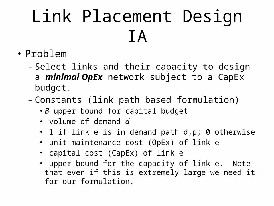
Link Placement Design IA

• Problem– Select links and their capacity to design a minimal

OpEx network subject to a CapEx budget.– Constants (link path based formulation)

• B upper bound for capital budget• volume of demand d• 1 if link e is in demand path d,p; 0 otherwise• unit maintenance cost (OpEx) of link e• capital cost (CapEx) of link e• upper bound for the capacity of link e. Note that even if

this is extremely large we need it for our formulation.

Link Placement Design IB

• Givens– List of candidate paths for each demand

• Variables– flow for demand d on its path p ()– capacity of link e ()– provisioning indicator 1 if used, 0 otherwise. Used

in CapEx bounds and capacity bounds.

Link Placement Design IC

• Objective– Minimize OpEx network costs– Minimize:

• CapEx budget Constraint

• Demand satisfaction Constraints– for

Link Placement Design ID

• Bandwidth Capacity Constraints

for • “Can’t use it if its not installed” Constraint

for – What does this do?– Remember that is 1 if the link is installed and zero

otherwise.

Example 1• Demands

– ('B14', 'B2'): 26.4, ('B5', 'B14'): 17.9, ('B5', 'B2'): 25.1, ('B5', 'B8'): 18.4, ('B8', 'B14'): 26.7

Example 1 CapEx Visualization(B7, B8): 264.97(B4, B5): 265.38(B0, B1): 313.45(B5, B9): 338.68(B6, B7): 364.00(B3, B5): 465.24(B3, B4): 488.41(B2, B0): 538.91(B2, B1): 636.99(B10, B9): 667.89(B12, B13): 765.40(B12, B8): 776.49(B11, B9): 888.73(B10, B11): 973.48(B4, B9): 1047.85(B14, B13): 1171.28(B5, B11): 1215.30(B3, B1): 1224.42(B3, B7): 1430.13(B2, B3): 1507.64(B8, B13): 1546.46

(B8, B13): 1546.46(B14, B12): 1726.92(B6, B8): 2042.67(B6, B0): 2066.16(B4, B8): 2273.53(B14, B10): 2371.38(B10, B13): 3058.32

CapEx based on length and a random multiplying integer– CapEx shown as width of dashed lines

Example 1: Results A• With a CapEx bound of 18,566.66• Optimum OpEx value of 50,116.57

Example 1: Results B• With a CapEx bound of 12,068.33 (lower)• Optimum OpEx value of 50,448.92 (bigger)

Example 1: Results C• With a CapEx bound of 11,140.00 (lower)• Optimum OpEx value of 51,250.81 (bigger)

Example 1: Results D• With a CapEx bound of 9,283.33 (lower)• Optimum OpEx value of 64,375.67 (bigger)

Optimizing both CapEx and OpEx

• What if we…– Want to optimize on CapEx?– Optimize on a combination of CapEx and OpEx– Find the minimum CapEx to produce a viable

network?• Can we reuse some of what we have?

Optimizing CapEx and OpEx

• Constants (link path based formulation)– B upper bound for capital budget– volume of demand d– 1 if link e is in demand path d,p; 0 otherwise– unit maintenance cost (OpEx) of link e– capital cost (CapEx) of link e– upper bound for the capacity of link e. Note that

even if this is extremely large we need it for our formulation.

Optimizing CapEx and OpEx

• Variables– flow for demand d on its path p ()– capacity of link e ()– provisioning indicator 1 if used, 0 otherwise. Used

in CapEx bounds and capacity bounds.

Optimizing CapEx and OpEx

• Objective– Minimize OpEx network costs– Minimize:

• CapEx budget Constraint

• Demand satisfaction Constraints– for

Optimizing CapEx and OpEx

• Bandwidth Capacity Constraints

for • “Can’t use it if its not installed” Constraint

for – What does this do?– Remember that is 1 if the link is installed and zero

otherwise.

Example• Result from minimization with previous CapEx values and OpEx

values scalled down by 0.01– Objective value = 9,283.33, used this as a basis for the CapEx bounds in

the previous formulation examples.