Embed Size (px)
Citation preview
B. TECH. PHYSICS LABORATORY MANUAL
2019-2020
DEPARTMENT OF PHYSICS
NATIONAL INSTITUTE OF TECHNOLOGY MANIPUR LANGOL, MANIPUR
1
B. Tech. Physics Lab Manual/NIT Manipur
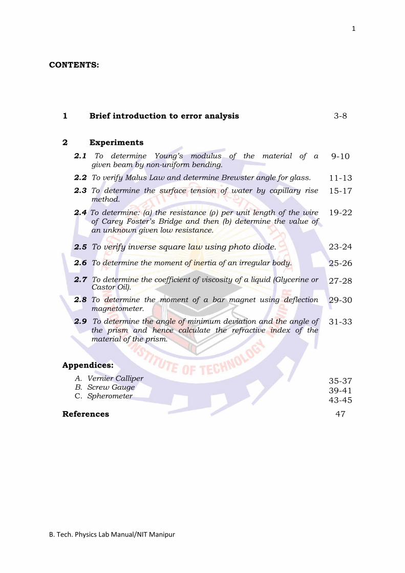
CONTENTS:
1 Brief introduction to error analysis
3-8
2 Experiments
2.1 To determine Young’s modulus of the material of a given beam by non-uniform bending.
9-10
2.2 To verify Malus Law and determine Brewster angle for glass. 11-13
2.3 To determine the surface tension of water by capillary rise method.
15-17
2.4 To determine: (a) the resistance (𝜌) per unit length of the wire of Carey Foster’s Bridge and then (b) determine the value of an unknown given low resistance.
19-22
2.5 To verify inverse square law using photo diode. 23-24
2.6 To determine the moment of inertia of an irregular body. 25-26
2.7 To determine the coefficient of viscosity of a liquid (Glycerine or Castor Oil).
27-28
2.8 To determine the moment of a bar magnet using deflection magnetometer.
29-30
2.9 To determine the angle of minimum deviation and the angle of the prism and hence calculate the refractive index of the material of the prism.
31-33
Appendices:
A. Vernier Calliper B. Screw Gauge C. Spherometer
35-37
39-41 43-45
References 47
2
B. Tech. Physics Lab Manual/NIT Manipur
3
B. Tech. Physics Lab Manual/NIT Manipur
BRIEF INTRODUCTION TO ERROR ANALYSIS
No measurement of a physical quantity can be entirely accurate. It is important to know,
therefore, just how much the measured value is likely to deviate from the unknown, true,
value of the quantity. The art of estimating these deviations should probably be called
uncertainty analysis, but for historical reasons is referred to as error analysis. This chapter
briefly discuss how errors are reported, kinds of errors that can occur, how to estimate
random errors, and how to carry error estimates into calculated results. We will not discuss
the “percent error” exercises common in high school, where the student is content with
calculating the deviation from some allegedly authoritative number.
Types of errors
There are three types of limitations to measurements:
1) Instrumental limitations
Any measuring device can only be used to measure to with a certain degree of fineness. Our
measurements are no better than the instruments we use to make them.
2) Systematic errors and blunders
These are caused by a mistake which does not change during the measurement. For example,
if the platform balance you used to weigh something was not correctly set to zero with no
weight on the pan, all your subsequent measurements of mass would be too large. Systematic
errors do not enter into the uncertainty. They are both identified and eliminated or lurk in the
background producing a shift from the true value.
3) Random errors
These arise from unnoticed variations in measurement technique, tiny changes in the
experimental environment, etc. Random variations affect precision. Truly random effects
average out if the results of a large number of trials are combined.
4) Absolute errors
The absolute error in a measured quantity is the uncertainty in the quantity and has the same
units as the quantity itself. For example, if you know a length is 0.428 m ± 0.002m, the 0.002
m is an absolute error.
5) Relative errors
The relative error (also called the fractional error) is obtained by dividing the absolute error
in the quantity by the quantity itself. The relative error is usually more significant than the
absolute error. For example, a 1 mm error in the diameter of a skate wheel is probably more
serious than a 1 mm error in a truck tire.
4
B. Tech. Physics Lab Manual/NIT Manipur
6) Percentage error
When reporting relative errors it is usual to multiply the fractional error by 100 and report it
as a percentage. It is known as percentage error.
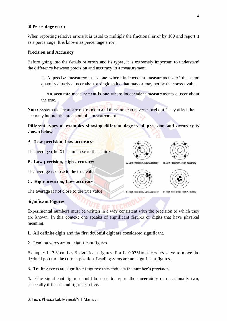
Precision and Accuracy
Before going into the details of errors and its types, it is extremely important to understand
the difference between precision and accuracy in a measurement.
A precise measurement is one where independent measurements of the same
quantity closely cluster about a single value that may or may not be the correct value.
An accurate measurement is one where independent measurements cluster about
the true.
Note: Systematic errors are not random and therefore can never cancel out. They affect the
accuracy but not the precision of a measurement.
Different types of examples showing different degrees of precision and accuracy is
shown below.
A. Low‐precision, Low‐accuracy:
The average (the X) is not close to the centre
B. Low‐precision, High‐accuracy:
The average is close to the true value
C. High‐precision, Low‐accuracy:
The average is not close to the true value
Significant Figures
Experimental numbers must be written in a way consistent with the precision to which they
are known. In this context one speaks of significant figures or digits that have physical
meaning.
1. All definite digits and the first doubtful digit are considered significant.
2. Leading zeros are not significant figures.
Example: L=2.31cm has 3 significant figures. For L=0.0231m, the zeros serve to move the
decimal point to the correct position. Leading zeros are not significant figures.
3. Trailing zeros are significant figures: they indicate the number’s precision.
4. One significant figure should be used to report the uncertainty or occasionally two,
especially if the second figure is a five.
5
B. Tech. Physics Lab Manual/NIT Manipur
Rounding Numbers
To keep the correct number of significant figures, numbers must be rounded off. The
discarded digit is called the remainder. There are three rules for rounding:
If the remainder is less than 5, drop the last digit. Rounding to one decimal
place: 5.346 → 5.3
If the remainder is greater than 5, increase the final digit by 1. Rounding to
one decimal place: 5.798 → 5.8
If the remainder is exactly 5 then round the last digit to the closest even
number.
This is to prevent rounding bias. Remainders from 1 to 5 are rounded down half the time and
remainders from 6 to 10 are rounded up the other half.
Rounding to one decimal place: 3.55 → 3.6, also 3.65 → 3.6
Systematic errors
Systematic errors arise from a flaw in the measurement scheme which is repeated each time a
measurement is made. If you do the same thing wrong each time you make the measurement,
your measurement will differ systematically (that is, in the same direction each time) from
the correct result. Some sources of systematic error are:
• Errors in the calibration of the measuring instruments.
• Incorrect measuring technique: For example, one might make an incorrect scale reading
because of parallax error.
• Bias of the experimenter. The experimenter might consistently read an instrument
incorrectly, or might let knowledge of the expected value of a result influence the
measurements.
It is clear that systematic errors do not average to zero if you average many measurements. If
a systematic error is discovered, a correction can be made to the data for this error. If you
measure a voltage with a meter that later turns out to have a 0.2 V offset, you can correct the
originally determined voltages by this amount and eliminate the error. Although random
errors can be handled more or less routinely, there is no prescribed way to find systematic
errors. One must simply sit down and think about all of the possible sources of error in a
given measurement, and then do small experiments to see if these sources are active. The
goal of a good experiment is to reduce the systematic errors to a value smaller than the
random errors. For example a meter stick should have been manufactured such that the
millimetre markings are positioned much more accurately than one millimetre.
6
B. Tech. Physics Lab Manual/NIT Manipur
Random errors
Random errors arise from the fluctuations that are most easily observed by making multiple
trials of a given measurement. For example, if you were to measure the period of a pendulum
many times with a stop watch, you would find that your measurements were not always the
same. The main source of these fluctuations would probably be the difficulty of judging
exactly when the pendulum came to a given point in its motion, and in starting and stopping
the stop watch at the time that you judge. Since you would not get the same value of the
period each time that you try to measure it, your result is obviously uncertain. There are
several common sources of such random uncertainties in the type of experiments that you are
likely to perform:
• Uncontrollable fluctuations in initial conditions in the measurements. Such
fluctuations are the main reason why, no matter how skilled the player, no individual
can toss a basketball from the free throw line through the hoop each and every time,
guaranteed. Small variations in launch conditions or air motion cause the trajectory to
vary and the ball misses the hoop.
• Limitations imposed by the precision of your measuring apparatus, and the
uncertainty in interpolating between the smallest divisions. The precision simply
means the smallest amount that can be measured directly. A typical meter stick is
subdivided into millimetres and its precision is thus one millimetre.
• Lack of precise definition of the quantity being measured. The length of a table in
the laboratory is not well defined after it has suffered years of use. You would find
different lengths if you measured at different points on the table. Another possibility
is that the quantity being measured also depends on an uncontrolled variable. (The
temperature of the object for example).
• Sometimes the quantity you measure is well defined but is subject to inherent
random fluctuations. Such fluctuations may be of a quantum nature or arise from the
fact that the values of the quantity being measured are determined by the statistical
behaviour of a large number of particles. Another example is AC noise causing the
needle of a voltmeter to fluctuate. No matter what the source of the uncertainty, to be
labelled "random" an uncertainty must have the property that the fluctuations from
some "true" value are equally likely to be positive or negative. This fact gives us a
key for understanding what to do about random errors. You could make a large
number of measurements, and average the result. If the uncertainties are really
equally likely to be positive or negative, you would expect that the average of a large
number of measurements would be very near to the correct value of the quantity
measured, since positive and negative fluctuations would tend to cancel each other.
7
B. Tech. Physics Lab Manual/NIT Manipur
Estimating random errors
There are several ways to make a reasonable estimate of the random error in a particular
measurement. The best way is to make a series of measurements of a given quantity (say, x)
and calculate the mean x , and the standard deviation σx from this data.
The mean is defined as
x = 1
N∑ xi
Ni=1
where xi is the result of the ith measurement and N is the number of measurements. The
standard deviation is given by
σx= [ 1
N∑ (xi
N
i=1− x)2 ]1/2
If a measurement (which is subject only to random fluctuations) is repeated many times,
approximately 68% of the measured valves will fall in the range x ± σx. We become more
certain that x , is an accurate representation of the true value of the quantity x, the more we
repeat the measurement. A useful quantity is therefore the standard deviation of the mean σx
defined as σx ≡ σx / N. The quantity σx is a good estimate of our uncertainty in x . Notice that
the measurement precision increases in proportion to N as we increase the number of
measurements. Not only have you made a more accurate determination of the value, you also
have a set of data that will allow you to estimate the uncertainty in your measurement.
Propagation of errors
Once you have some experimental measurements, you usually combine them according to
some formula to arrive at a desired quantity. To find the estimated error (uncertainty) for a
calculated result one must know how to combine the errors in the input quantities. The
simplest procedure would be to add the errors. This would be a conservative assumption, but
it overestimates the uncertainty in the result. Clearly, if the errors in the inputs are random,
they will cancel each other at least some of the time. If the errors in the measured quantities
are random and if they are independent (that is, if one quantity is measured as being, say,
larger than it really is, another quantity is still just as likely to be smaller or larger) then error
theory shows that the uncertainty in a calculated result (the propagated error) can be obtained
from a few simple rules, some of which are listed in Table 1. For example if two or more
numbers are to be added (Table 1.2) then the absolute error in the result is the square root of
the sum of the squares of the absolute errors of the inputs, i.e.
if z = x+y
then Δz=[(Δx)2+(Δy)2]1/2
In this and the following expressions, ∆x and ∆y are the absolute random errors in x and y
and ∆z is the propagated uncertainty in z. The formulas do not apply to systematic errors.
The general formula, for your information, is the following;
8
B. Tech. Physics Lab Manual/NIT Manipur
(Δf (x1,x2,K))2 = ∑ (dy/dx)2 (Δxi)2
It is discussed in detail in many texts on the theory of errors and the analysis of experimental
data. For now, the collection of formulae on the next page will suffice.
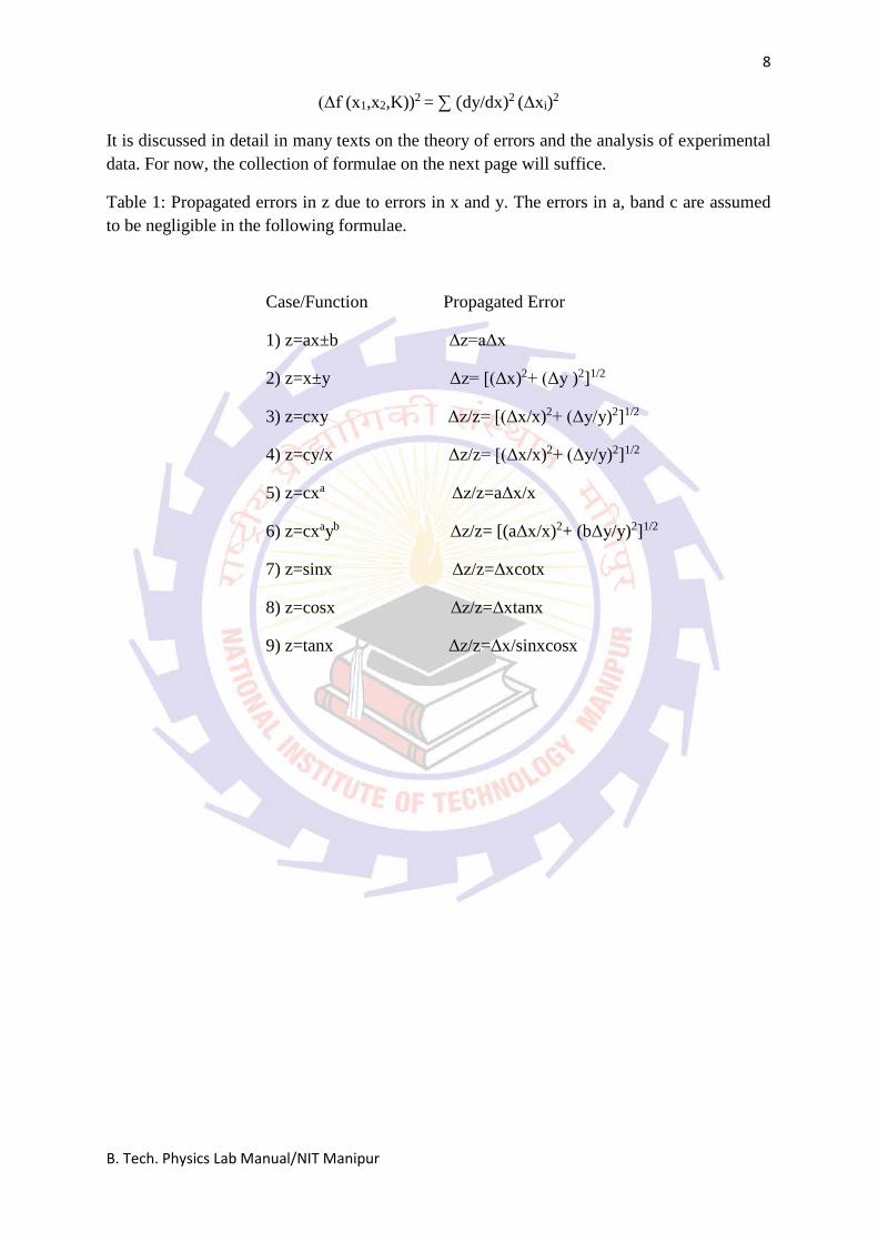
Table 1: Propagated errors in z due to errors in x and y. The errors in a, band c are assumed
to be negligible in the following formulae.
Case/Function Propagated Error
1) z=ax±b Δz=aΔx
2) z=x±y Δz= [(Δx)2+ (Δy )2]1/2
3) z=cxy Δz/z= [(Δx/x)2+ (Δy/y)2]1/2
4) z=cy/x Δz/z= [(Δx/x)2+ (Δy/y)2]1/2
5) z=cxa Δz/z=aΔx/x
6) z=cxayb Δz/z= [(aΔx/x)2+ (bΔy/y)2]1/2
7) z=sinx Δz/z=Δxcotx
8) z=cosx Δz/z=Δxtanx
9) z=tanx Δz/z=Δx/sinxcosx
9
B. Tech. Physics Lab Manual/NIT Manipur
Experiment no.: 2.1
Aim of the experiment: To determine Young’s Modulus of the material of a
given beam by non-uniform bending.
Materials required:
a. Two knife edge supports
b. Weight hanger with set of weights
c. Vernier callipers
d. Screw gauge
e. Three types of Bar (Iron Bar, Brass Bar & Aluminium Bar)
f. Buzzer
Principle:
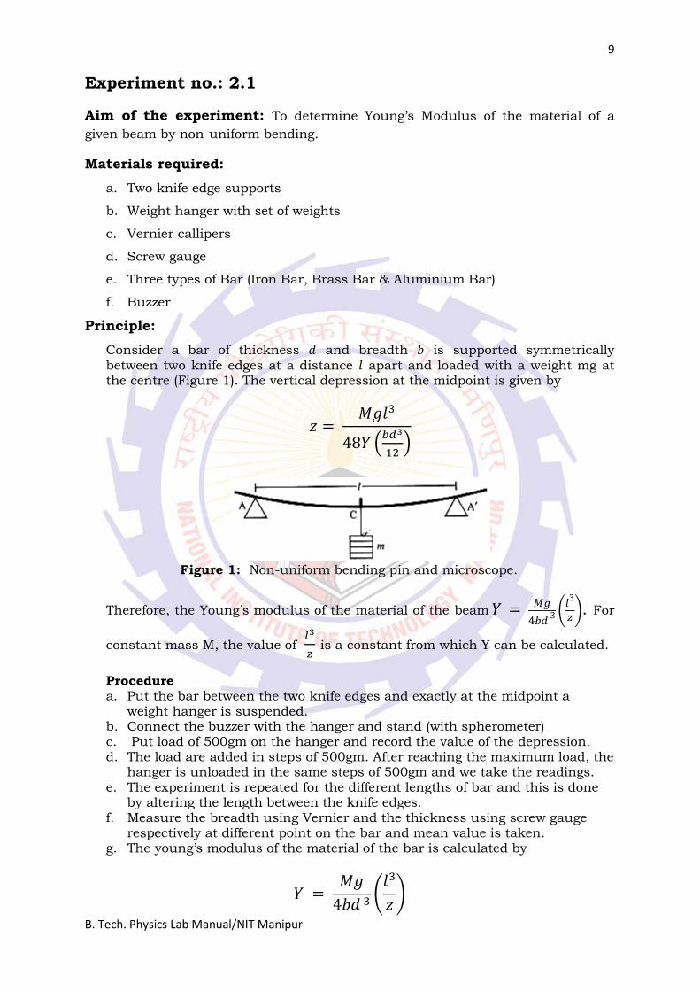
Consider a bar of thickness 𝑑 and breadth 𝑏 is supported symmetrically
between two knife edges at a distance 𝑙 apart and loaded with a weight mg at the centre (Figure 1). The vertical depression at the midpoint is given by
𝑧 = 𝑀𝑔𝑙3
48𝑌 (𝑏𝑑3
12)
Figure 1: Non-uniform bending pin and microscope.
Therefore, the Young’s modulus of the material of the beam 𝑌 = 𝑀𝑔
4𝑏𝑑 3 (
𝑙3
𝑧). For
constant mass M, the value of 𝑙3
𝑧 is a constant from which Y can be calculated.
Procedure a. Put the bar between the two knife edges and exactly at the midpoint a
weight hanger is suspended. b. Connect the buzzer with the hanger and stand (with spherometer) c. Put load of 500gm on the hanger and record the value of the depression. d. The load are added in steps of 500gm. After reaching the maximum load, the
hanger is unloaded in the same steps of 500gm and we take the readings. e. The experiment is repeated for the different lengths of bar and this is done
by altering the length between the knife edges. f. Measure the breadth using Vernier and the thickness using screw gauge
respectively at different point on the bar and mean value is taken. g. The young’s modulus of the material of the bar is calculated by
𝑌 = 𝑀𝑔
4𝑏𝑑 3(
𝑙3
𝑧)
10
B. Tech. Physics Lab Manual/NIT Manipur
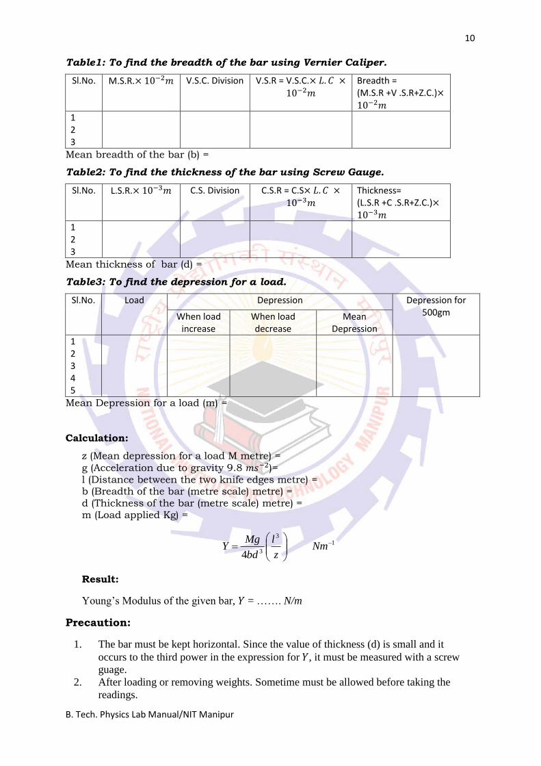
Table1: To find the breadth of the bar using Vernier Caliper.
Sl.No. M.S.R.× 10−2𝑚 V.S.C. Division V.S.R = V.S.C.× 𝐿. 𝐶 ×
10−2𝑚
Breadth = (M.S.R +V .S.R+Z.C.)×10−2𝑚
1 2 3
Mean breadth of the bar (b) =
Table2: To find the thickness of the bar using Screw Gauge.
Sl.No. L.S.R.× 10−3𝑚 C.S. Division C.S.R = C.S× 𝐿. 𝐶 ×10−3𝑚
Thickness= (L.S.R +C .S.R+Z.C.)×10−3𝑚
1 2 3
Mean thickness of bar (d) =
Table3: To find the depression for a load.
Sl.No. Load Depression Depression for 500gm When load
increase When load decrease
Mean Depression
1 2 3 4 5
Mean Depression for a load (m) =
Calculation:
z (Mean depression for a load M metre) =
g (Acceleration due to gravity 9.8 𝑚𝑠−2)= l (Distance between the two knife edges metre) = b (Breadth of the bar (metre scale) metre) = d (Thickness of the bar (metre scale) metre) = m (Load applied Kg) =
13
34
Nm
z
l
bd
MgY
Result:
Young’s Modulus of the given bar, 𝑌 = ……. N/m
Precaution:
1. The bar must be kept horizontal. Since the value of thickness (d) is small and it
occurs to the third power in the expression for 𝑌, it must be measured with a screw
guage.
2. After loading or removing weights. Sometime must be allowed before taking the
readings.
11
B. Tech. Physics Lab Manual/NIT Manipur
Experiment no.:2.2
Aim of the experiment: To verify Malus Law and determine Brewster angle for glass.
Materials required:
1. Lamp 40 watt
2. Photo diode
3. Digital Current Meter
4. Two polariod
5. Glass plate
6. Spectrometer
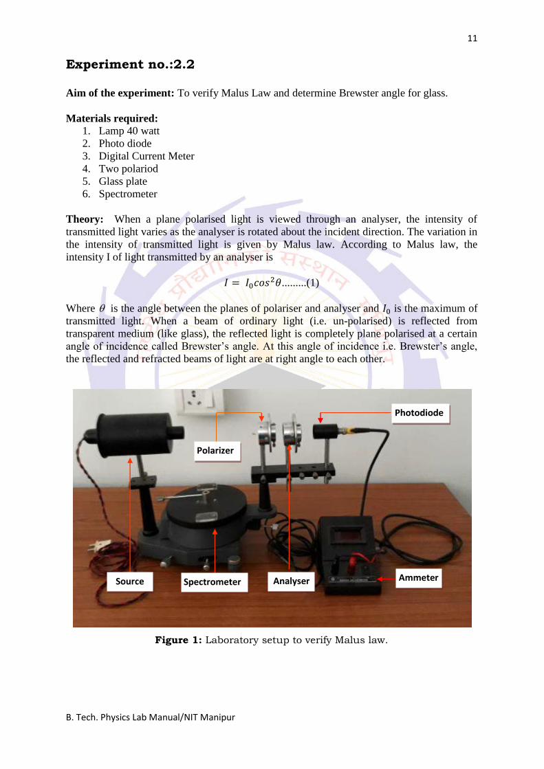
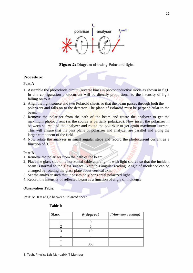
Theory: When a plane polarised light is viewed through an analyser, the intensity of
transmitted light varies as the analyser is rotated about the incident direction. The variation in
the intensity of transmitted light is given by Malus law. According to Malus law, the
intensity I of light transmitted by an analyser is
𝐼 = 𝐼0𝑐𝑜𝑠2𝜃.........(1)
Where is the angle between the planes of polariser and analyser and 𝐼0 is the maximum of
transmitted light. When a beam of ordinary light (i.e. un-polarised) is reflected from
transparent medium (like glass), the reflected light is completely plane polarised at a certain
angle of incidence called Brewster’s angle. At this angle of incidence i.e. Brewster’s angle,
the reflected and refracted beams of light are at right angle to each other.
Figure 1: Laboratory setup to verify Malus law.
Ammeter
Photodiode
Analyser Spectrometer
Polarizer
Source
12
B. Tech. Physics Lab Manual/NIT Manipur
Figure 2: Diagram showing Polarised light
Procedure:
Part A
1. Assemble the photodiode circuit (reverse bias) in photoconductive mode as shown in fig1.
In this configuration photocurrent will be directly proportional to the intensity of light
falling on to it.
2. Align the light source and two Polaroid sheets so that the beam passes through both the
polarizers and falls on to the detector. The plane of Polaroid must be perpendicular to the
beam.
3. Remove the polarizer from the path of the beam and rotate the analyzer to get the
maximum photocurrent (as the source is partially polarized). Now insert the polarizer in
between source and the analyzer and rotate the polarizer to get again maximum current.
This will ensure that the pass plane of polarizer and analyzer are parallel and along the
larger component of the field.
4. Now rotate the analyzer in small angular steps and record the photocurrent current as a
function of .
Part B
1. Remove the polarizer from the path of the beam.
2. Place the glass slab on a horizontal table and align it with light source so that the incident
beam is normal to the glass surface. Note this angular reading. Angle of incidence can be
changed by rotating the glass plate about vertical axis.
3. Set the analyzer such that it passes only horizontal polarized light.
4. Record the intensity of reflected beam as a function of angle of incidence.
Observation Table:
Part A: = angle between Polaroid sheet
Table I:
Sl.no. 𝜃(𝑑𝑒𝑔𝑟𝑒𝑒) I(Ammeter reading)
1 0
2 5
3 10
.. ..
.. ..
.. 360
13
B. Tech. Physics Lab Manual/NIT Manipur
Part B: I = Angle of incidence
Table II:
Sl.no. 𝜃I(𝑑𝑒𝑔𝑟𝑒𝑒) I(Ammeter reading)
1 10
2 15
3 20
4 25
.. ..
.. 80
Analysis:
Part A: Plot 2cosVsI and verify eqn. (1).
Part B:, Plot IVsI . Find Brewster angle from the minima of the graph.
Results:
Brewster’s angle for glass = … … … … (degree/rad)

14
B. Tech. Physics Lab Manual/NIT Manipur
15
B. Tech. Physics Lab Manual/NIT Manipur
Experiment no.:2.3 Aim of the experiment: To determine the surface tension of water by capillary rise method.
Materials required: 1. Capillary tube
2. A beaker containing water 3. Travelling microscope 4. Pointer
5. Clamp stand
Principle:
Surface tension of a liquid is defined as the force per unit length acting on either side of a line drawn in the liquid surface in equilibrium, the direction
of the force being tangential to the surface and perpendicular to the line.
If ′𝜌′ be the density of water, which rises to a height ‘h’ by capillary tube of
radius ‘r’, then the surface tension of water is given by
𝑆 =1
2 𝑔𝑟𝜌(ℎ +
𝑟
3)
Where, g is the acceleration due to gravity. (For water ,the angle of contact
𝜃 = 0) Procedure: A clean capillary tube is arranged in a vertical position with its lower end
dipping in water. Due to capillarity water level within the tube will rise up. A pointer is held such that its lower tip just touches on the surface of the
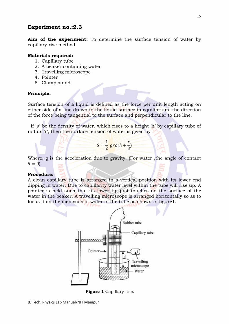
water in the beaker. A travelling microscope is arranged horizontally so as to focus it on the meniscus of water in the tube as shown in figure1.
Figure 1 Capillary rise.
16
B. Tech. Physics Lab Manual/NIT Manipur
17
B. Tech. Physics Lab Manual/NIT Manipur

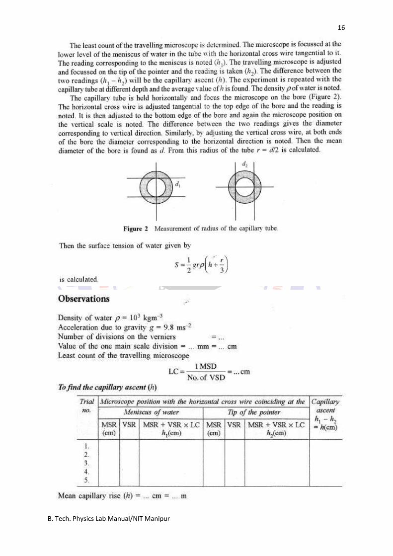
18
B. Tech. Physics Lab Manual/NIT Manipur
19
B. Tech. Physics Lab Manual/NIT Manipur
Experiment no.:2.4
Aim of the experiment: To determine (a) the resistance (𝜌) per unit length of the wire
of Carey Foster’s Bridge and then (b) determine the value of an unknown given low
resistance.
Materials required:
1. Carry Foster Bridge with four gap set up.
2. Two Fixed Resistance of 2 Ohm.
3. Two equal fractional Resistance box 0.1 to 2 Ohm.
4. Galvanometer 30-0-30 Division Sensitivity of 20𝜇A/Division (Model No. ME 471D).
5. One Way Key
6. Battery Eliminator 2-6V/2Amps.(Model No. ME 402).
7. DCC Wire (Connecting Wire)
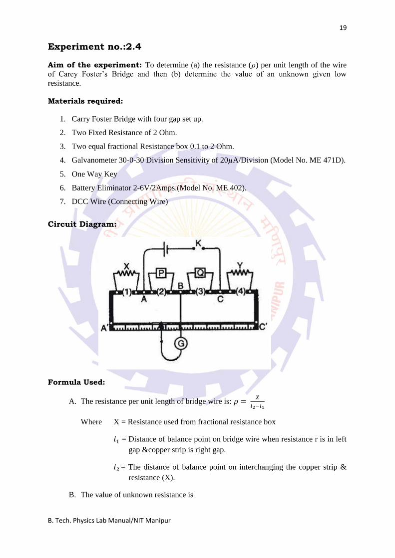
Circuit Diagram:
Formula Used:
A. The resistance per unit length of bridge wire is: 𝜌 = 𝑋
𝑙2−𝑙1
Where X = Resistance used from fractional resistance box
𝑙1 = Distance of balance point on bridge wire when resistance r is in left
gap &copper strip is right gap.
𝑙2 = The distance of balance point on interchanging the copper strip &
resistance (X).
B. The value of unknown resistance is
20
B. Tech. Physics Lab Manual/NIT Manipur
Y = X – (𝑙2 − 𝑙1)𝜌
Procedure:
Part A: Determination of resistance per unit length, 𝝆 of the Carey Foster’s bridge wire
1. Make the circuit connections as shown in Figure. In this part of the experiment Y is a
copper strip that has negligible resistance and X is a fractional resistance box. You
need to ensure that the wires and copper strip are clean and the terminals are screwed
down tightly, (b) remove any deposits from the battery terminals and (c) close tightly
all of the plugs in the resistance box; these precautions will minimize any contact
resistance between the terminals and the connecting wire.
2. Plug in the battery key so that a current flows through the bridge. Note that you
should remove the battery plug when you are not taking measurements.
3. Press down the jockey so that the knife edge makes contact with the wire, and
observe the galvanometer deflection. Release the jockey.
4. Move the jockey to different positions along the wire and repeat step 3 at each place
until you locate the position of the null point, where there is no deflection of the
Galvanometer. This point should be near the middle of the bridge wire. Take care that
the jockey is pressed down gently to avoid damaging the wire and distorting its cross
section, and do not move the jockey while it is in contact with the wire.
5. Note the balancing length, l1, in your laboratory notebook, using a table with the
layout shown in Table 1.
6. Reverse the connections to the terminals of the battery and record the balancing
length for reverse current in the table in your notebook. By averaging readings with
forward and reverse currents, you will be able to eliminate the effect of any thermo
emfs.
7. Take out the plug from the fractional resistance box that inserts a resistance of 0.1 , and repeat steps 3 – 5.
8. Increase resistance X in steps of 0.1 and repeat steps 3 – 5 each time.
9. Interchange the copper strip and fractional resistance box, and repeat steps 3 – 5 for
the same set of resistances. The corresponding balancing lengths, measured from the
same end of the bridge wire, should be recorded as l2 in your data table.
10. Calculate the resistance per unit length using the formula,𝜌 =𝑋
𝑙2−𝑙1
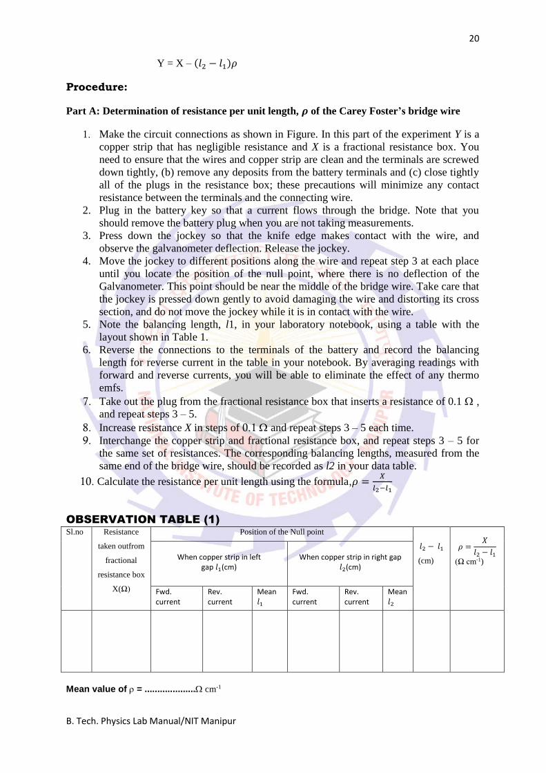
OBSERVATION TABLE (1) Sl.no Resistance
taken outfrom
fractional
resistance box
X(Ω)
Position of the Null point
𝑙2 − 𝑙1
(cm)
𝜌 =𝑋
𝑙2 − 𝑙1
(Ω cm-1)
When copper strip in left
gap 𝑙1(cm)
When copper strip in right gap
𝑙2(cm)
Fwd. current
Rev. current
Mean 𝑙1
Fwd. current
Rev. current
Mean 𝑙2
Mean value of = ....................cm-1
21
B. Tech. Physics Lab Manual/NIT Manipur
Part B: Determination of an unknown low resistance Y
1. After calculating the resistance per unit length of the wire from the first part (a) now
remove the copper strip and insert the unknown low resistance in one of the outer
gaps of the bridge.
2. Repeat the entire sequences of steps 1 to 9 as described in the procedure from the first
part of the experiment. Record your measurements in your laboratory notebook. A
suggested format is shown in Table 2.
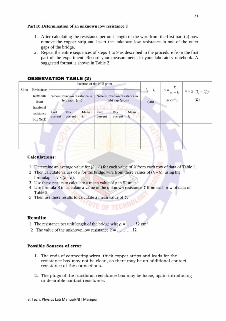
OBSERVATION TABLE (2)
Sl.no
Resistance
taken out
from
fractional
resistance
box X(Ω)
Position of the Null point
𝑙2 − 𝑙1
(cm)
𝜌 =𝑋
𝐼2 − 𝐼1
(Ω cm-1)
Y = X -(𝑙2 − 𝑙1)𝜌
(Ω)
When Unknown resistance in
left gap 𝑙1(cm)
When Unknown resistance in
right gap 𝑙2(cm)
Fwd. current
Rev. current
Mean 𝑙1
Fwd. current
Rev. current
Mean 𝑙2
Calculations:
1 Determine an average value for (l2 – l1) for each value of X from each row of data of Table 1.
2 Then calculate values of for the bridge wire from these values of (l2 – l1), using the
formula= X / (l2 – l1).
3 Use these results to calculate a mean value of in SI units. 4 Use formula B to calculate a value of the unknown resistance Y from each row of data of
Table 2. 5 Then use these results to calculate a mean value of Y.
Results:
1 The resistance per unit length of the bridge wire = …… cm-1
2 The value of the unknown low resistance Y = ………..
Possible Sources of error:
1. The ends of connecting wires, thick copper strips and leads for the
resistance box may not be clean, so there may be an additional contact resistance at the connections.
2. The plugs of the fractional resistance box may be loose, again introducing
undesirable contact resistance.
22
B. Tech. Physics Lab Manual/NIT Manipur
3. The bridge wire may get heated up due to continuous passage of current for
a long time. This will change its resistance.
4. If the jockey is not pressed gently or if it is kept pressed on to the wire while being shifted from one point to another, that may alter the cross sectional area of the wire and make it non uniform.
23
B. Tech. Physics Lab Manual/NIT Manipur
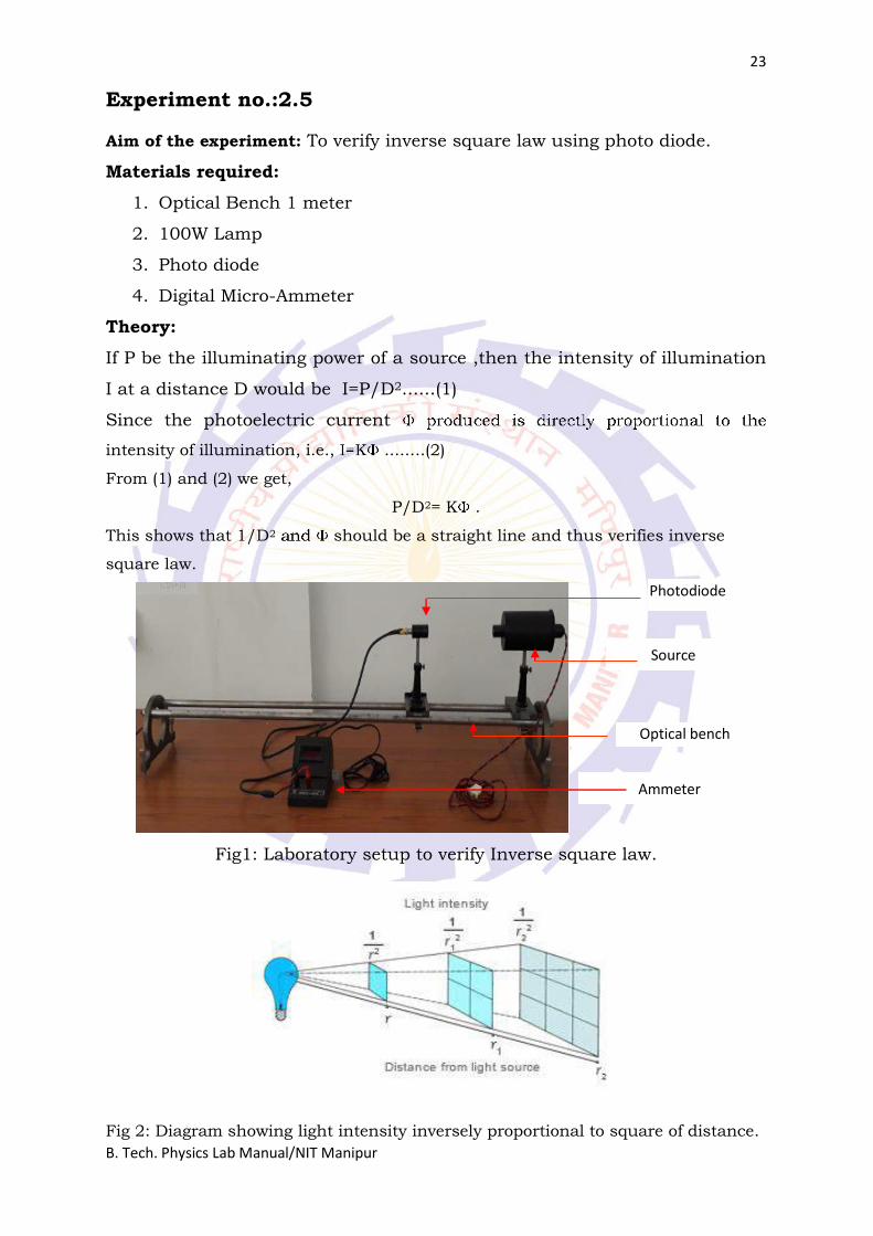
Experiment no.:2.5
Aim of the experiment: To verify inverse square law using photo diode.
Materials required:
1. Optical Bench 1 meter
2. 100W Lamp
3. Photo diode
4. Digital Micro-Ammeter
Theory:
If P be the illuminating power of a source ,then the intensity of illumination
I at a distance D would be I=P/D2......(1)
Since the photoelectric current
intensity of illumination, i.e., ........(2)
From (1) and (2) we get,
P/D2= K .
This shows that 1/D2 should be a straight line and thus verifies inverse
square law.
Fig1: Laboratory setup to verify Inverse square law.
Fig 2: Diagram showing light intensity inversely proportional to square of distance.
Photodiode
Source
Ammeter
Optical bench
24
B. Tech. Physics Lab Manual/NIT Manipur
Procedure:
1. The experiment can be performed in the laboratory but it is always better to
perform it in a dark room where stray light falling on the photo diode can be
avoided. In the dark room mount the various parts of the apparatus on the
optical bench i.e., place the lamp and photo diode on optical bench facing
towards each other.
2. Connect the photodiode to the Digital Micro Ammeter provided.
3. Set the micro meter at 𝜇𝐴 mode and adjust lamp at particular position say
0cm with the help of scale marked on optical bench.
4. Switch on the lamp and set photo diode at 15cm from the source. Record
the meter reading.
5. Take observation for different set of distance between lamp and photo diode
as shown in observation table.
Observation:
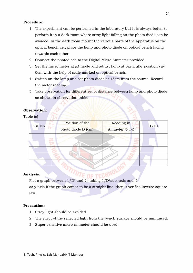
Table (a)
Sl. No. Position of the
photo diode D (cm)
Reading in
(𝜇𝐴) 1/D2
Analysis:
Plot a graph between 1/D2 and , taking 1/D2as x-axis and
as y-axis.If the graph comes to be a straight line ,then it verifies inverse square
law.
Precaution:
1. Stray light should be avoided.
2. The effect of the reflected light from the bench surface should be minimised.
3. Super sensitive micro-ammeter should be used.
25
B. Tech. Physics Lab Manual/NIT Manipur
Experiment no.:2.6
Aim of the experiment: To determine the moment of inertia of an irregular body.
Materials required:
a. Moment of Inertia setup
b. Stop watch
c. Spirit level
d. Metal block (rectangular or circular)
e. Vernier Calliper Theory:
The moment of inertia 𝐼2 of the irregular body
is given by 𝐼2 = 𝐼1 × 𝑇2
2− 𝑇2
𝑇12−𝑇2
T = time period for table alone
T1= time period for table + regular body
T2= time period for table + body whose mom. of inertia is required
I1= moment of inertia of a regular body
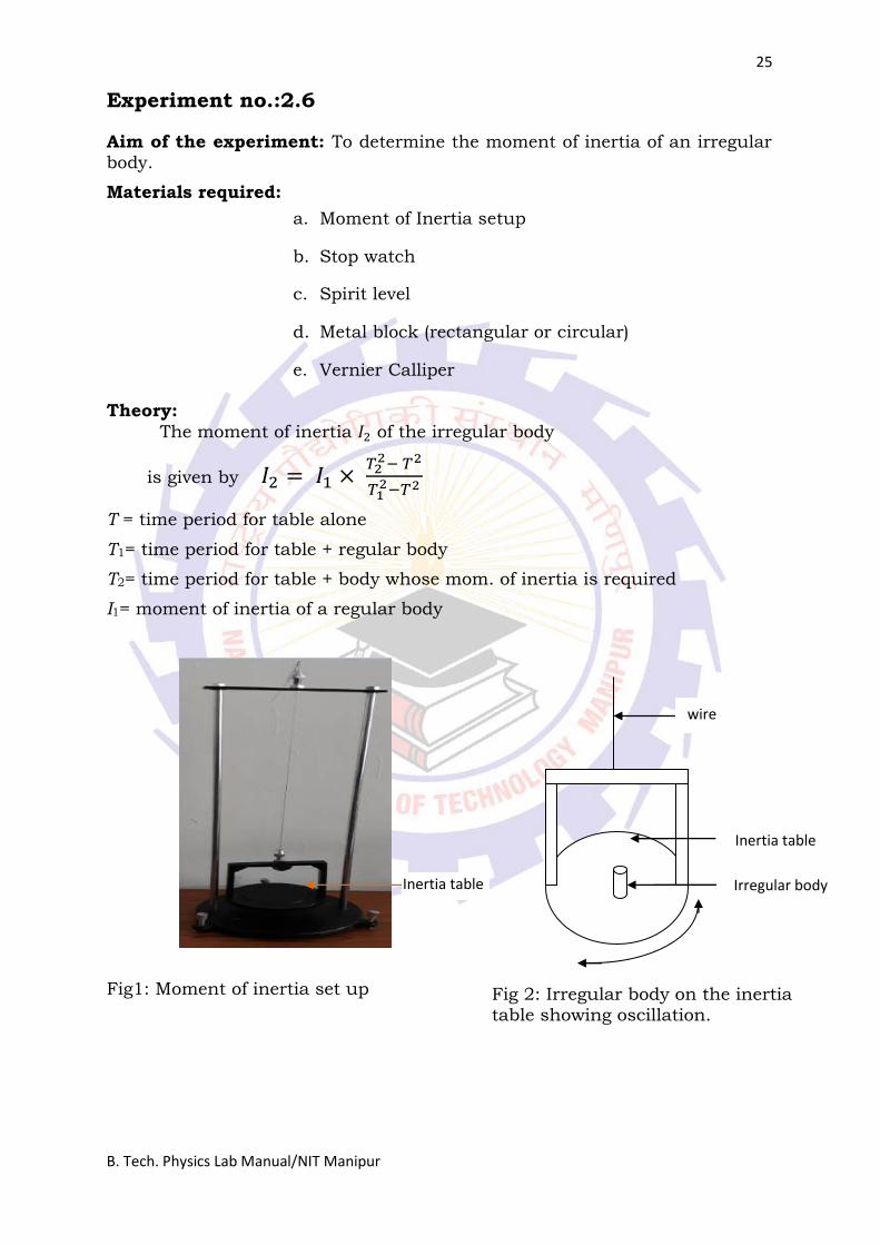
Fig1: Moment of inertia set up
Inertia table
Inertia table
Irregular body
wire
Fig 2: Irregular body on the inertia table showing oscillation.
26
B. Tech. Physics Lab Manual/NIT Manipur
Procedure:
1. Make the base of inertia table horizontal as shown in fig 1. 2. Make the table horizontal with the help of small weights. 3. Slightly rotate the table in its own plane and release it in such a way that it oscillates without moving as a whole, find the time taken by 10, 15, 20, and 30 oscillations and thereby time period T
𝑇 = 𝑇𝑜𝑡𝑎𝑙 𝑡𝑖𝑚𝑒
𝑁𝑜. 𝑜𝑓 𝑜𝑠𝑐𝑖𝑙𝑙𝑎𝑡𝑖𝑜𝑛𝑠
4. Put the irregular body on the inertia table and find time period𝑻𝟐
5. Remove the irregular body and place the regular body (circular metal
block) on the inertia table whose moment of inertia is known by its
dimensions. Thus find time period𝑻𝟏
6. Weigh the regular body and note the mass M.
7. Find the diameter of the block with the help of Vernier callipers and
calculate its radius R.
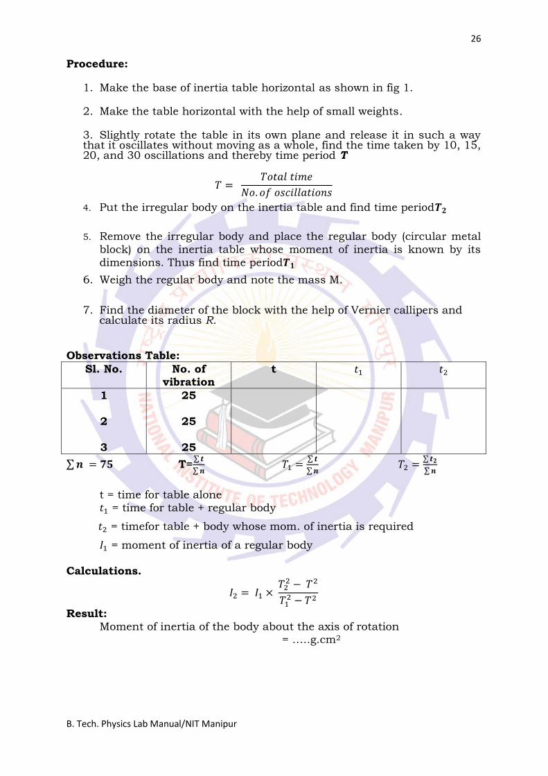
Observations Table:
Sl. No. No. of vibration
t 𝑡1 𝑡2
1 2
3
25
25
25
∑ 𝒏 = 𝟕𝟓 T=∑ 𝒕
∑ 𝒏 𝑇1 =
∑ 𝒕
∑ 𝒏 𝑇2 =
∑ 𝒕𝟐
∑ 𝒏
t = time for table alone
𝑡1 = time for table + regular body
𝑡2 = timefor table + body whose mom. of inertia is required
𝐼1 = moment of inertia of a regular body Calculations.
𝐼2 = 𝐼1 × 𝑇2
2 − 𝑇2
𝑇12 − 𝑇2
Result: Moment of inertia of the body about the axis of rotation = …..g.cm2
27
B. Tech. Physics Lab Manual/NIT Manipur
Experiment no.:2.7
Aim of the experiment: To determine the Coefficient of Viscosity of a Liquid
(e.g., Glycerine or Castor Oil)
Material:
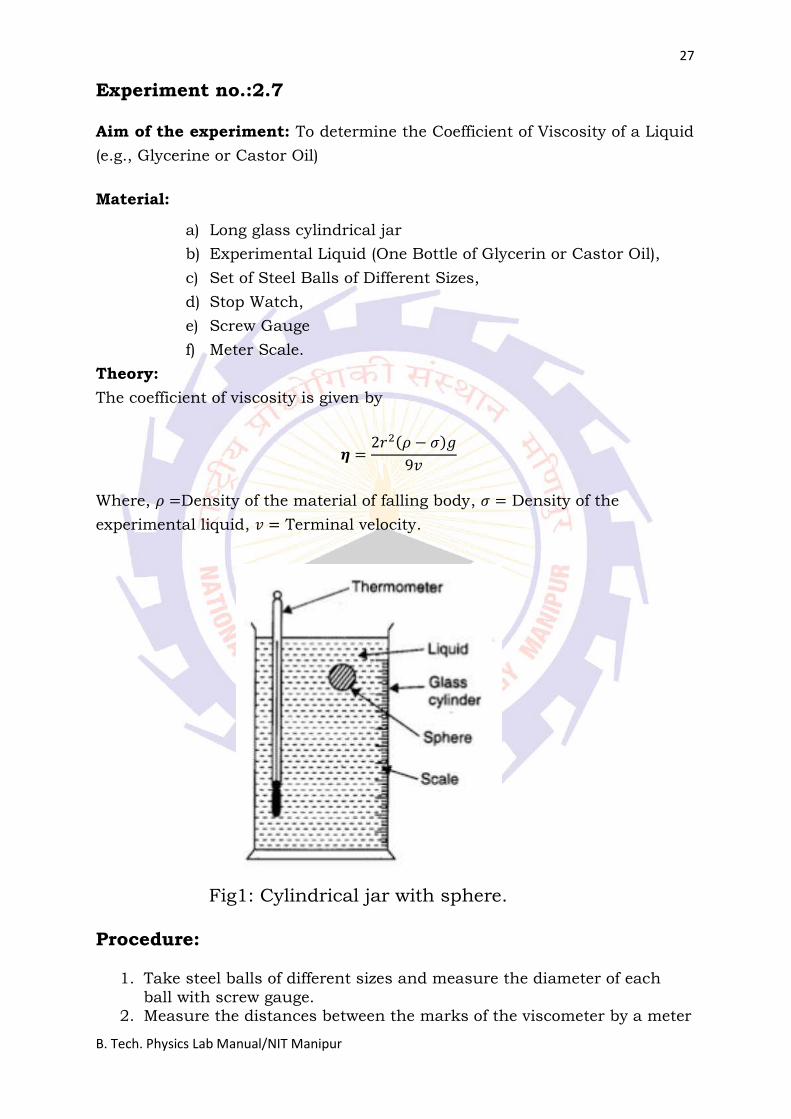
a) Long glass cylindrical jar
b) Experimental Liquid (One Bottle of Glycerin or Castor Oil),
c) Set of Steel Balls of Different Sizes,
d) Stop Watch,
e) Screw Gauge
f) Meter Scale.
Theory:
The coefficient of viscosity is given by
𝜼 =2𝑟2(𝜌 − 𝜎)𝑔
9𝑣
Where, 𝜌 =Density of the material of falling body, 𝜎 = Density of the
experimental liquid, 𝑣 = Terminal velocity.
Fig1: Cylindrical jar with sphere. Procedure:
1. Take steel balls of different sizes and measure the diameter of each
ball with screw gauge. 2. Measure the distances between the marks of the viscometer by a meter
28
B. Tech. Physics Lab Manual/NIT Manipur
scale. 3. Drop one ball in the viscometer and keep eye on the level of uppermost
mark. As soon as the ball crosses this mark, start the stop watch. Carefully note down the times t1 and t2 for descending heights h1 and h2 respectively.
4. Repeat the above procedure for different balls. 5. Using a sensitive thermometer, record the temperature of the
experimental liquid.
Observations: Terminal velocity of spherical ball
Distance fallen h1 = …..cm, h2 = ……..cm
Time taken t1 = ……s , t2 =……….s
Calculations:
𝜼 =2𝑟2(𝜌 − 𝜎)𝑔
9𝑣
Result:
The coefficient of viscosity of the liquid at temperature
(𝜃°𝐶) = ⋯ 𝐶. 𝐺. 𝑆. 𝑢𝑛𝑖𝑡𝑠
Precautions (to be taken):
1. Liquid should be transparent to watch motion of the ball.
2. Ball should be perfectly spherical.
3. Velocity should be noted only when it becomes constant.
Sources of Error:
1. The liquid may not have uniform density
2. The ball may not be perfectly spherical
3. The noted velocity may not be constant.
29
B. Tech. Physics Lab Manual/NIT Manipur
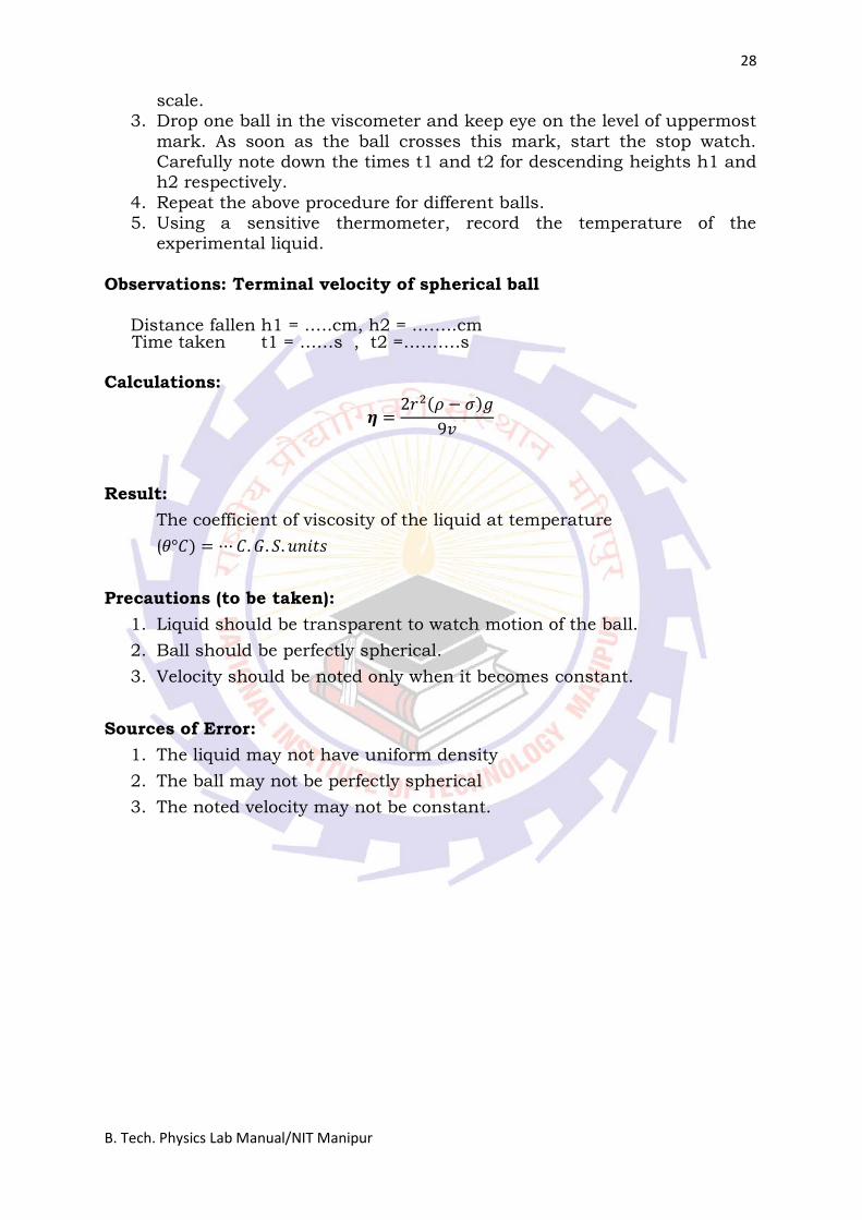
Experiment no.:2.8
Aim of the experiment: To determine the moment of a bar magnet usin deflection magnetometer.
Materials required:
a. Deflection magnetometer
b. Bar magnet
c. vernier callipers etc.
Principle:
The magnetic flux density at a distance d due to a bar magnet when arranged in
tan A position is
𝜇0
4𝜋
2𝑀𝑑
(𝑑2 − 𝑙2)2= 𝐵𝐻𝑡𝑎𝑛𝜃
Where M is the moment of the magnet.
𝐵𝐻 is the horizontal component of the earth’s magnetic flux density.
𝜃 is the deflecting angle and 𝑙 is the half length of the magnet and is equal to ½(actual length of the magnet X 0.85)
The numerical values of
𝐵𝐻 = 0.38 × 10⁻⁴𝑇
𝜇0 = 4𝜋 × 10−7𝐻𝑚−1 Therefore, the moment of the magnet
𝑀 = 107(𝑑2 − 𝑙2)2
2𝑑𝐵𝐻𝑡𝑎𝑛𝜃
Fig 1: Deflection magnetometer
Procedure:
1. All magnets and magnetic substances are far removed from the working table.
Magnet in tan A position
Compass needle
30
B. Tech. Physics Lab Manual/NIT Manipur
2. The deflection magnetometer is placed on the working table with its two arms perpendicular to the magnetic meridian i.e., perpendicular to the magnetic to the axis of the magnetic needle (so that the needle is at the end on position or ‘Tan A position’ with respect to the magnet, while the two arms are aligned with the magnetic ‘east west’ direction). The pointer is
made to read the (00 − 00). 3. The magnet is now put on the east arm of the magnetometer, aligned with
the arm itself and adjusted so that the pointer reads about 450 on the circular scale. The readings d1 and d2 corresponding to the two ends of the magnet are noted from the scale fixed on the arm.
4. The distance of the centre of the needle from the centre of the magnet is then given by,
𝑑 = 𝑑1 + 𝑑2
2
5. Keeping the distance ‘d’ fixed the readings of the two ends of the pointer are noted When (i) the two flat surfaces of the magnet are alternately touching the arm and (ii) the N-pole and S-pole of the magnet are alternately pointing towards the needle. Thus, altogether we get eight readings.
6. The magnet is then transferred to the ‘west-arm’. Keeping the magnet at the
equal distance ‘d’, operation (5) is again repeated, giving again eight readings. The mean of these 16 readings gives the deflection (𝜃) of the needle for that particular distance‘d’.
7. The magnet is next placed in turn at two other distances, until the
deflections are about 430 and470. The corresponding distances are given each by the mean of the scale readings of the two ends of the magnet.
Observations
Horizontal component of the earth’s magnetic flux density 𝐵𝐻 = ⋯ 𝑇 Half length of the magnet 𝑙 = …m To find M in tan A position
Trial No.
Distance between
centres of the magnet and
compass needle d(m)
Deflection 𝑀 = 107
(𝑑2 − 𝑙2)2
2𝑑𝐵𝐻𝑡𝑎𝑛𝜃
(𝐴𝑚2)
1 2 3 4 5 6 7 8 Mean 𝜃
1. 2. 3. 4. 5.
Mean value of magnetic moment in tan A position = ….𝐴𝑚2
Result
Moment of the magnet in
tan A position = …..𝐴𝑚2
31
B. Tech. Physics Lab Manual/NIT Manipur
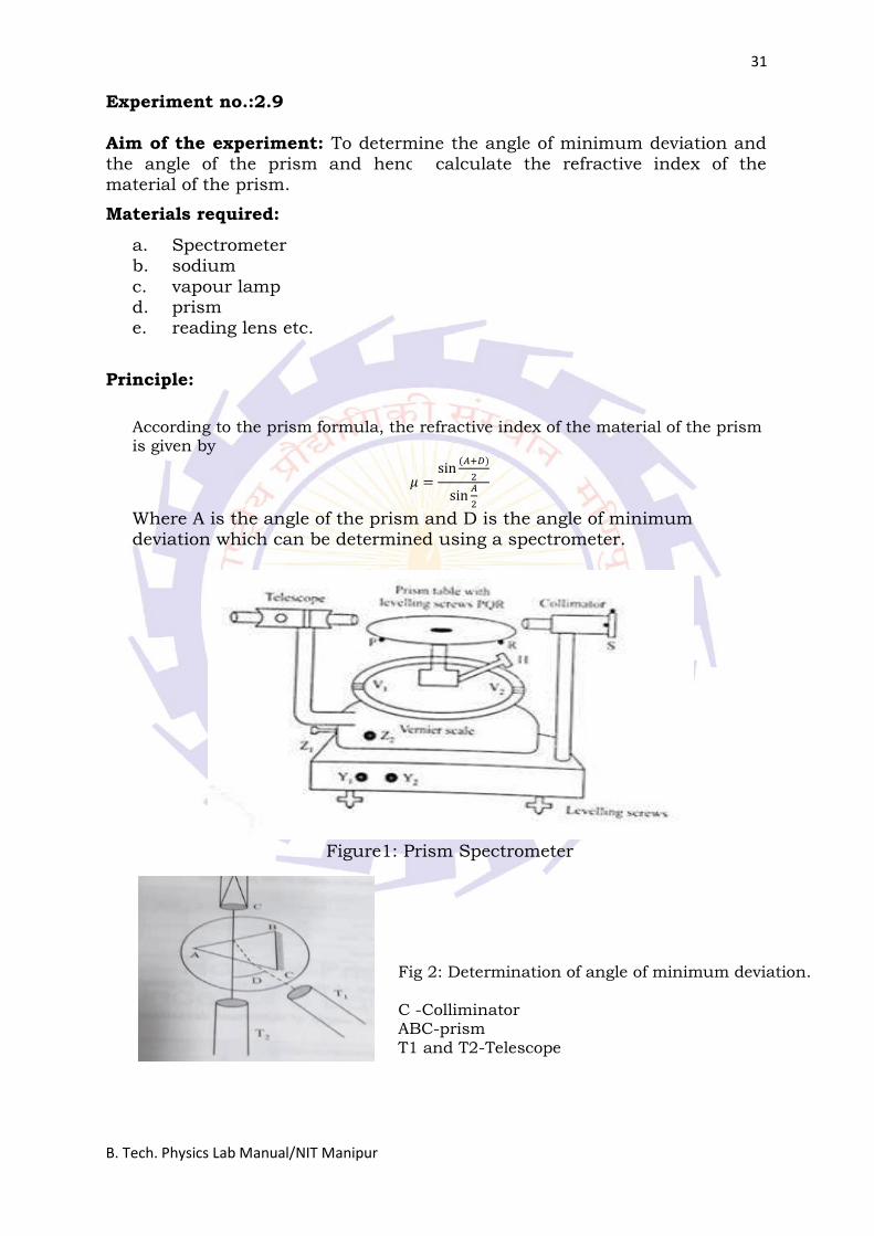
Experiment no.:2.9
Aim of the experiment: To determine the angle of minimum deviation and the angle of the prism and hence calculate the refractive index of the material of the prism.
Materials required:
a. Spectrometer b. sodium
c. vapour lamp d. prism e. reading lens etc.
Principle:
According to the prism formula, the refractive index of the material of the prism is given by
𝜇 =sin
(𝐴+𝐷)
2
sin𝐴
2
Where A is the angle of the prism and D is the angle of minimum deviation which can be determined using a spectrometer.
Figure1: Prism Spectrometer
Fig 2: Determination of angle of minimum deviation. C -Colliminator ABC-prism T1 and T2-Telescope
32
B. Tech. Physics Lab Manual/NIT Manipur
Procedure: To find the angle of the prism A
1. The prism table is clamped at a suitable height. 2. The prism ABC is placed on
a) The apex almost at the centre. b) The base BC of the prism towards the prism table clamp. c) The side AB of the prism is perpendicular to the parallel lines inscribed
on the table. 3. The prism table (or the vernier table) is rotated such that the edge A of the
prism is directed towards the collimator so that the light falls uniformly on both the faces. Clamp the vernier table in this position. Turn the telescope so that the reflected image from the first face (say AB) is viewed, and record both the verniers at that position.
4. Now turn the telescope towards the second face (say AC) and view the image and record both verniers. The difference of both faces gives 2A.Thus,the angle of prism is calculated.
To determine the angle of minimum deviation (D) 1. The prism table is rotated till the base of the prism is parallel to the axis of
the collimator. Now the light incident on the face AB and emerges through the face AC. Look with eye, the refracted image through the face AC and rotate the prism table in such a way that the refracted image moves towards the axial line of the collimator and then retraces.
2. View the refracted image through the telescope. Width of the slit is made narrow as possible. Clamp the vernier table and slightly rotate it by working the tangential screw of the collimator (or the prism table) on both sides where the refracted image is stationary. The cross wire of the telescope is made coincide exactly on the retracing point of the image adjusting its radial and tangential screws and the telescope readings corresponding two vernier are noted as refracted image readings.
3. Without disturbing the vernier table, the prism is removed. Turn the telescope to view the direct image and the readings corresponding to the direct images on both verniers are also noted. The difference between the refracted and the direct ray gives the angle of minimum deviation is found as D.
4. The refractive index of the material of the prism is then calculated using the formula
𝜇 =sin
(𝐴+𝐷)
2
sin𝐴
2
Observations:
To find the least count of the spectrometer
Value of main scale division on the rotation scale of the spectrometer = ….. degrees
No. of divisions on the vernier =
Least count LC = 1𝑀𝑆𝐷
𝑉𝑆𝐷 = ….. degree
33
B. Tech. Physics Lab Manual/NIT Manipur
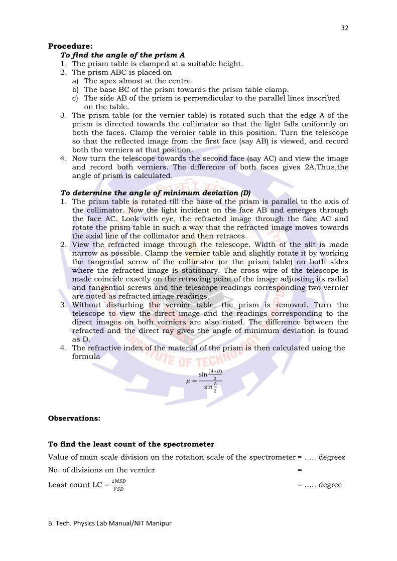
To find the angle of the prism (A)
Telescope reading ( in degrees) MSR +VSR × LC
x1˜x2=2A
First face (x1) Second face (x2)
Ver. I Ver. II Ver. I Ver. II
The angle of prism (A)=............
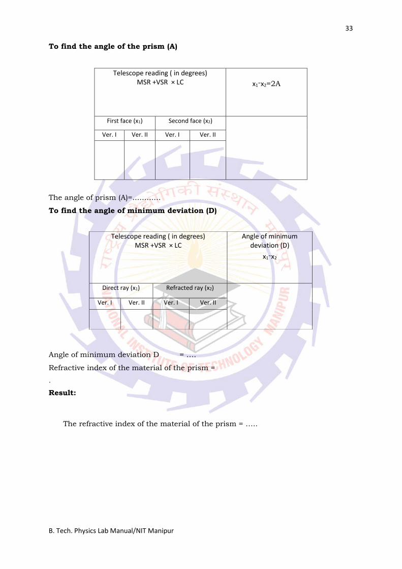
To find the angle of minimum deviation (D)
Angle of minimum deviation D = ….
Refractive index of the material of the prism =
.
Result:
The refractive index of the material of the prism = …..
Telescope reading ( in degrees) MSR +VSR × LC
Angle of minimum deviation (D)
x1˜x2
Direct ray (x1) Refracted ray (x2)
Ver. I Ver. II Ver. I Ver. II

34
B. Tech. Physics Lab Manual/NIT Manipur
35
B. Tech. Physics Lab Manual/NIT Manipur
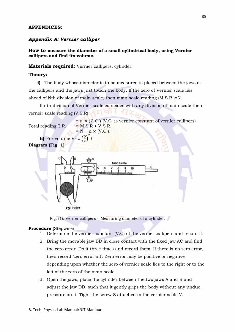
APPENDICES:
Appendix A: Vernier calliper
How to measure the diameter of a small cylindrical body, using Vernier
callipers and find its volume.
Materials required: Vernier callipers, cylinder.
Theory:
i) The body whose diameter is to be measured is placed between the jaws of
the callipers and the jaws just touch the body. If the zero of Vernier scale lies
ahead of Nth division of main scale, then main scale reading (M.S.R.)=N.
If nth division of Vernier scale coincides with any division of main scale then
verneir scale reading (V.S.R)
= 𝑛 × (𝑉. 𝐶. ) (V.C. is vernier constant of vernier callipers) Total reading T.R. = M.S.R + V.S.R.
= N + n × (V.C.).
ii) For volume V= 𝜋 (𝐷
2)
2𝑙
Diagram (Fig. 1)
Fig. (1). Verner callipers – Measuring diameter of a cylinder.
Procedure (Stepwise)
1. Determine the vernier constant (V.C) of the vernier callipers and record it.
2. Bring the movable jaw BD in close contact with the fixed jaw AC and find
the zero error. Do it three times and record them. If there is no zero error,
then record ‘zero error nil’.[Zero error may be positive or negative
depending upon whether the zero of vernier scale lies to the right or to the
left of the zero of the main scale]
3. Open the jaws, place the cylinder between the two jaws A and B and
adjust the jaw DB, such that it gently grips the body without any undue
pressure on it. Tight the screw S attached to the vernier scale V.
36
B. Tech. Physics Lab Manual/NIT Manipur
4. Note the position of the zero mark of the vernier scale on the main scale. Record the main scale reading just before the zero mark of the vernier scale. This reading (N) is called main scale reading (M.S.R.).
5. Note the number (n) of the vernier scale division which coincides with some division of the main scale and calculate Total reading T.R. = M.S.R + V.S.R.
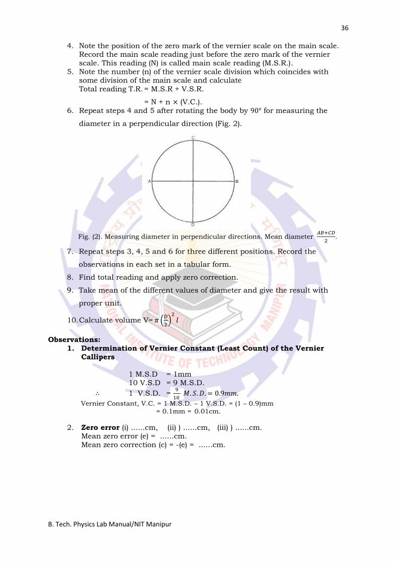
= N + n × (V.C.). 6. Repeat steps 4 and 5 after rotating the body by 90° for measuring the
diameter in a perpendicular direction (Fig. 2).
Fig. (2). Measuring diameter in perpendicular directions. Mean diameter 𝐴𝐵+𝐶𝐷
2.
7. Repeat steps 3, 4, 5 and 6 for three different positions. Record the
observations in each set in a tabular form.
8. Find total reading and apply zero correction.
9. Take mean of the different values of diameter and give the result with
proper unit.
10. Calculate volume V= 𝜋 (𝐷
2)
2𝑙
Observations:
1. Determination of Vernier Constant (Least Count) of the Vernier Callipers
1 M.S.D = 1mm 10 V.S.D = 9 M.S.D.
∴ 1 V.S.D. = 9
10 𝑀. 𝑆. 𝐷. = 0.9𝑚𝑚.
Vernier Constant, V.C. = 1 M.S.D. – 1 V.S.D. = (1 – 0.9)mm
= 0.1mm = 0.01cm.
2. Zero error (i) ......cm, (ii) ) ......cm, (iii) ) ......cm. Mean zero error (e) = ......cm. Mean zero correction (c) = -(e) = ......cm.
37
B. Tech. Physics Lab Manual/NIT Manipur
Calculations:
Mean corrected diameter
D = 𝐷1(𝑎)+D1(b)+𝐷2(𝑎)+D2(b)+𝐷3(𝑎)+D3(b)
6
And volume V= 𝜋 (𝐷
2)
2𝑙
Result
The diameter of the given cylinder is ..... cm and volume is......cm3.
Precautions (to be taken)
1. Motion of vernier scale on main scale should be made smooth (by oiling if
necessary).
2. Vernier contant and zero error should be carefully found and properly
recorded.
3. The body should be gripped between the jaws firmly but gently (without
undue pressure on it from the jaws).
4. Observations should be taken at right angles at one place and taken at least
as three different places.
Sources of Error
1. The vernier scale may be loose on main scale.
2. The jaws may not be at right angles to the main scale.
3. The graduations on scale may not be correct and clear.
4. Parallax may be there in taking observations.

38
B. Tech. Physics Lab Manual/NIT Manipur
39
B. Tech. Physics Lab Manual/NIT Manipur
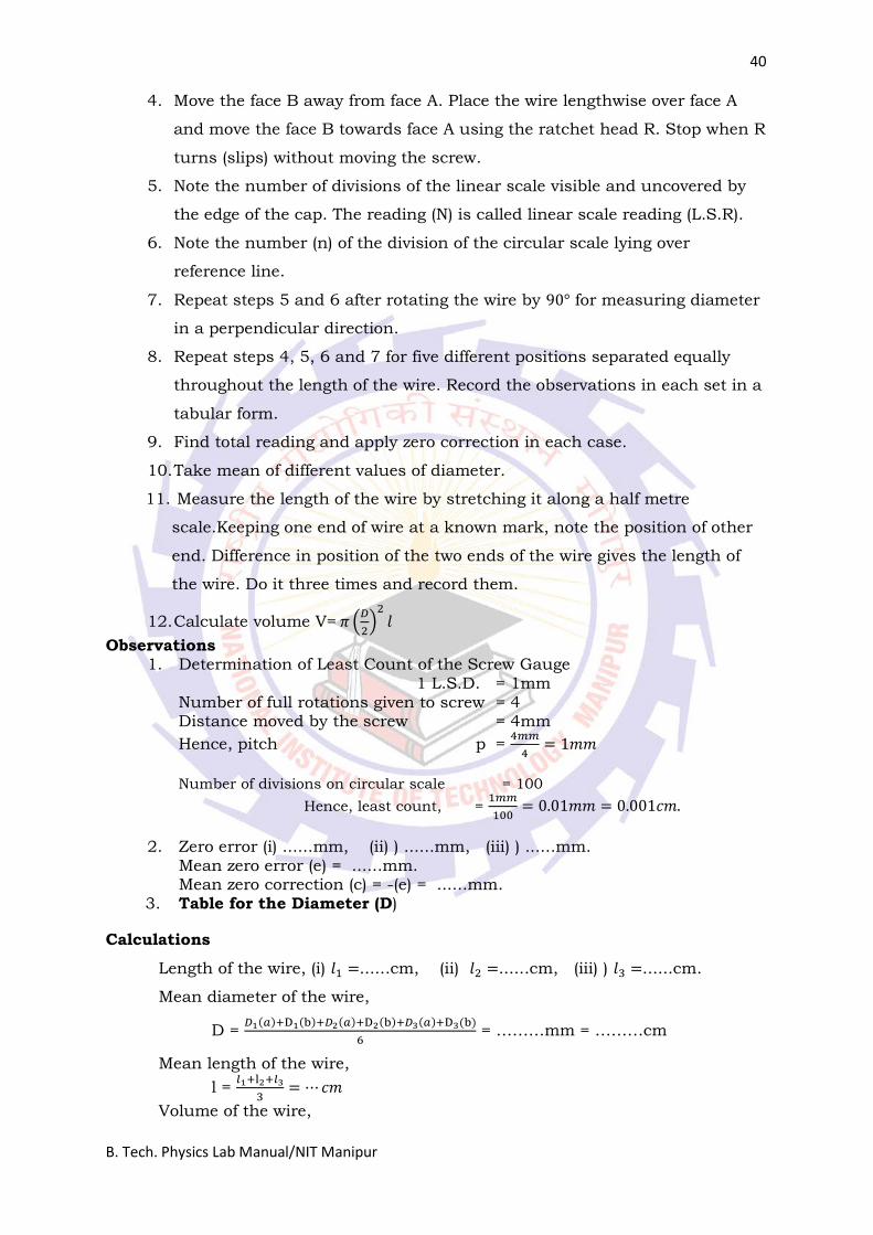
Appendix B: Screw gauge
How to measure diameter of a given wire using a screw gauge and find its
volume.
Materials required: Screw gauge, wire, half metre scale.
Theory:
1. The wire whose diameter is to measured is placed between the plane faces
A and B. If the edge of the cap lies ahead of Nth division of linear scale.
Then, linear main scale reading (L.S.R.) = N.
If nth division of circular scale lies over reference line.
Then, circular scale reading (C.S.R) = n x (L.C) (L.C is least count of screw
gauge).
Total reading (T.R.) = L.S.R. + C.S.R. = N + n × (L.C.).
2. If D be the diameter and l be the mean length of the wire. Then
Volume of the wire, V = 𝜋 (𝐷
2)
2𝑙.
Diagram (Fig. 1)
Fig. (1). Screw gauge – Measuring diameter (thickness) of the wire.
Procedure (Stepwise)
1. Find the value of one linear scale division (L.S.D).
2. Determine the pitch and the least count of the screw guage and record it
stepwise.
3. Bring the plane face B in contact with plane face A and find the zero error.
Do it three times and record them. If there is no zero error, then record
‘zero error nil’.[When faces A and B of screw gauge come in contact and
zero of circular scale does not cross the reference line, zero error is
positive. If the zero is positive. If the zero crosses the reference line, zero
error is negative]
40
B. Tech. Physics Lab Manual/NIT Manipur
4. Move the face B away from face A. Place the wire lengthwise over face A
and move the face B towards face A using the ratchet head R. Stop when R
turns (slips) without moving the screw.
5. Note the number of divisions of the linear scale visible and uncovered by
the edge of the cap. The reading (N) is called linear scale reading (L.S.R).
6. Note the number (n) of the division of the circular scale lying over
reference line.
7. Repeat steps 5 and 6 after rotating the wire by 90° for measuring diameter
in a perpendicular direction.
8. Repeat steps 4, 5, 6 and 7 for five different positions separated equally
throughout the length of the wire. Record the observations in each set in a
tabular form.
9. Find total reading and apply zero correction in each case.
10. Take mean of different values of diameter.
11. Measure the length of the wire by stretching it along a half metre
scale.Keeping one end of wire at a known mark, note the position of other
end. Difference in position of the two ends of the wire gives the length of
the wire. Do it three times and record them.
12. Calculate volume V= 𝜋 (𝐷
2)
2𝑙
Observations 1. Determination of Least Count of the Screw Gauge
1 L.S.D. = 1mm Number of full rotations given to screw = 4 Distance moved by the screw = 4mm
Hence, pitch p = 4𝑚𝑚
4= 1𝑚𝑚
Number of divisions on circular scale = 100
Hence, least count, = 1𝑚𝑚
100= 0.01𝑚𝑚 = 0.001𝑐𝑚.
2. Zero error (i) ......mm, (ii) ) ......mm, (iii) ) ......mm. Mean zero error (e) = ......mm. Mean zero correction (c) = -(e) = ......mm.
3. Table for the Diameter (D)
Calculations
Length of the wire, (i) 𝑙1 =......cm, (ii) 𝑙2 =......cm, (iii) ) 𝑙3 =......cm.
Mean diameter of the wire,
D = 𝐷1(𝑎)+D1(b)+𝐷2(𝑎)+D2(b)+𝐷3(𝑎)+D3(b)
6 = ………mm = ………cm
Mean length of the wire,
l = 𝑙1+l2+𝑙3
3= ⋯ 𝑐𝑚
Volume of the wire,
41
B. Tech. Physics Lab Manual/NIT Manipur
V = 𝜋 (𝐷
2)
2𝑙 =……cm3.
Result
The length of the wire is........and the volume of the given wire is..... cm3.
Precautions (to be taken)
1. To avoid undue pressure; the screw should always be rotated by ratchet R
and not by cap K.
2. The screw should move freely without friction.
3. The zero correction, with proper sign should be noted very carefully and
added algebraically.
4. For same set of observations, the screw should be moved in the same
direction to avoid back - lash error of the screw.
5. At each place, the diameter of the wire should be measured in two
perpendicular directions.
6. Readings should be taken at least for five different places equally spaced
along the whole length of the wire.
7. Error due to parallax should be avoided.
Sources of Error
1. The screw may have friction.
2. The screw gauge may have back – lash error.
3. Circular scale divisions may not be of equal size.
4. The wire may not be uniform.
42
B. Tech. Physics Lab Manual/NIT Manipur
43
B. Tech. Physics Lab Manual/NIT Manipur
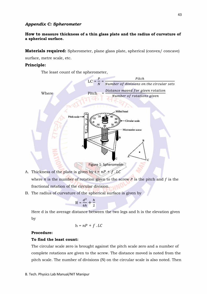
Appendix C: Spherometer
How to measure thickness of a thin glass plate and the radius of curvature of
a spherical surface.
Materials required: Spherometer, plane glass plate, spherical (convex/ concave)
surface, metre scale, etc.
Principle:
The least count of the spherometer,
LC = 𝑃
𝑁 =
𝑃𝑖𝑡𝑐ℎ
𝑁𝑢𝑚𝑏𝑒𝑟 𝑜𝑓 𝑑𝑖𝑣𝑖𝑠𝑖𝑜𝑛𝑠 𝑜𝑛 𝑡ℎ𝑒 𝑐𝑖𝑟𝑐𝑢𝑙𝑎𝑟 𝑠𝑒𝑡𝑠
Where Pitch = 𝐷𝑖𝑠𝑡𝑎𝑛𝑐𝑒 𝑚𝑜𝑣𝑒𝑑 𝑓𝑜𝑟 𝑔𝑖𝑣𝑒𝑛 𝑟𝑜𝑡𝑎𝑡𝑖𝑜𝑛
𝑁𝑢𝑚𝑏𝑒𝑟 𝑜𝑓 𝑟𝑜𝑡𝑎𝑡𝑖𝑜𝑛𝑠 𝑔𝑖𝑣𝑒𝑛
Figure 1: Spherometer.
A. Thickness of the plate is given by t = 𝑛𝑃 + 𝑓 . 𝐿𝐶
where 𝑛 is the number of rotation given to the screw 𝑃 is the pitch and 𝑓 is the
fractional rotation of the circular division.
B. The radius of curvature of the spherical surface is given by
R = 𝑑2
6ℎ+
ℎ
2
Here d is the average distance between the two legs and h is the elevation given
by
h = 𝑛𝑃 + 𝑓 . 𝐿𝐶
Procedure:
To find the least count:
The circular scale zero is brought against the pitch scale zero and a number of
complete rotations are given to the screw. The distance moved is noted from the
pitch scale. The number of divisions (N) on the circular scale is also noted. Then
44
B. Tech. Physics Lab Manual/NIT Manipur
Pitch = 𝐷𝑖𝑠𝑡𝑎𝑛𝑐𝑒 𝑚𝑜𝑣𝑒𝑑 𝑓𝑜𝑟 𝑔𝑖𝑣𝑒𝑛 𝑟𝑜𝑡𝑎𝑡𝑖𝑜𝑛
𝑁𝑢𝑚𝑏𝑒𝑟 𝑜𝑓 𝑟𝑜𝑡𝑎𝑡𝑖𝑜𝑛𝑠 𝑔𝑖𝑣𝑒𝑛
And Least count (LC) = 𝑃𝑖𝑡𝑐ℎ
𝑁𝑢𝑚𝑏𝑒𝑟 𝑜𝑓 𝑑𝑖𝑣𝑖𝑠𝑖𝑜𝑛𝑠 𝑜𝑛 𝑡ℎ𝑒 𝑐𝑖𝑟𝑐𝑢𝑙𝑎𝑟 𝑠𝑒𝑡𝑠
are calculated.
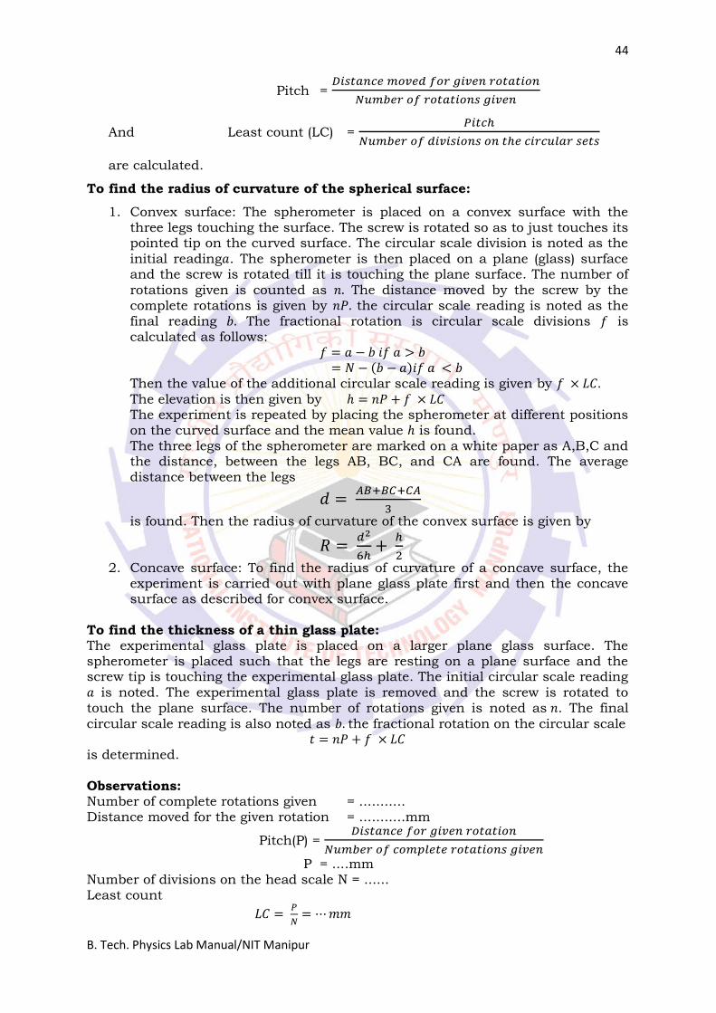
To find the radius of curvature of the spherical surface:
1. Convex surface: The spherometer is placed on a convex surface with the three legs touching the surface. The screw is rotated so as to just touches its pointed tip on the curved surface. The circular scale division is noted as the
initial reading𝑎. The spherometer is then placed on a plane (glass) surface and the screw is rotated till it is touching the plane surface. The number of
rotations given is counted as 𝑛. The distance moved by the screw by the complete rotations is given by 𝑛𝑃. the circular scale reading is noted as the final reading 𝑏. The fractional rotation is circular scale divisions 𝑓 is
calculated as follows: 𝑓 = 𝑎 − 𝑏 𝑖𝑓 𝑎 > 𝑏 = 𝑁 − (𝑏 − 𝑎)𝑖𝑓 𝑎 < 𝑏 Then the value of the additional circular scale reading is given by 𝑓 × 𝐿𝐶. The elevation is then given by ℎ = 𝑛𝑃 + 𝑓 × 𝐿𝐶
The experiment is repeated by placing the spherometer at different positions on the curved surface and the mean value ℎ is found. The three legs of the spherometer are marked on a white paper as A,B,C and the distance, between the legs AB, BC, and CA are found. The average distance between the legs
𝑑 = 𝐴𝐵+𝐵𝐶+𝐶𝐴
3
is found. Then the radius of curvature of the convex surface is given by
𝑅 = 𝑑2
6ℎ+
ℎ
2
2. Concave surface: To find the radius of curvature of a concave surface, the experiment is carried out with plane glass plate first and then the concave surface as described for convex surface.
To find the thickness of a thin glass plate: The experimental glass plate is placed on a larger plane glass surface. The spherometer is placed such that the legs are resting on a plane surface and the screw tip is touching the experimental glass plate. The initial circular scale reading
𝑎 is noted. The experimental glass plate is removed and the screw is rotated to touch the plane surface. The number of rotations given is noted as 𝑛. The final
circular scale reading is also noted as 𝑏. the fractional rotation on the circular scale 𝑡 = 𝑛𝑃 + 𝑓 × 𝐿𝐶
is determined.
Observations: Number of complete rotations given = ........... Distance moved for the given rotation = ...........mm
Pitch(P) = 𝐷𝑖𝑠𝑡𝑎𝑛𝑐𝑒 𝑓𝑜𝑟 𝑔𝑖𝑣𝑒𝑛 𝑟𝑜𝑡𝑎𝑡𝑖𝑜𝑛
𝑁𝑢𝑚𝑏𝑒𝑟 𝑜𝑓 𝑐𝑜𝑚𝑝𝑙𝑒𝑡𝑒 𝑟𝑜𝑡𝑎𝑡𝑖𝑜𝑛𝑠 𝑔𝑖𝑣𝑒𝑛
P = ....mm Number of divisions on the head scale N = ...... Least count
𝐿𝐶 = 𝑃
𝑁= ⋯ 𝑚𝑚
45
B. Tech. Physics Lab Manual/NIT Manipur
Distance between the legs AB = ... mm, BC = ...mm, CA = ..mm Mean distance between the legs
𝑑 = 𝐴𝐵+𝐵𝐶+𝐶𝐴
3 = ...mm
Calculation:
(1) 𝑡 = 𝑛𝑃 + 𝑓 × 𝐿𝐶
(2) 𝑅 = 𝑑2
6ℎ+
ℎ
2
Result: Thickness of the glass plate = ...m Radius of curvature of the spherical surface = ...m Precautions:
1. The screw should move freely without friction.
2. The screw should be moved in same direction to avoid back-lash error of
the screw.
3. Excess rotation should be avoided.
Sources of Error:
1. The screw may have friction.
2. The spherometer may have back – lash error.
3. Circular (Disc) scale divisions may not be of equal size.

46
B. Tech. Physics Lab Manual/NIT Manipur
47
B. Tech. Physics Lab Manual/NIT Manipur
References:
1. Comprehensive Practical Physics by J.N.Jaiswal and
Dr.Rajendra Singh.
2. Advanced Practical Physics by Samir Kumar Ghosh.
3. Practical Physics by P.R. Sasi Kumar.
4. Practical Physics by Harnam Singh.
5. Practical Physics by Indu Prakash Ramakrishna.