H O S T E D B Y The Japanese Geotechnical Society

Soils and Foundations

Soils and Foundations 2015;55(2):315–328

http://d0038-0

nCorTongjifax: þ8

E-mPeer

x.doi.org/806/& 201

respondinUniversi6 21 659ail addrereview un

.sciencedirect.come: www.elsevier.com/locate/sandf

wwwjournal homepag

Axial capacity degradation of single piles in soft clay under cyclic loading

Maosong Huanga,b,n, Ying Liua,b,c

aDepartment of Geotechnical Engineering, Tongji University, Shanghai 200092, ChinabKey Laboratory of Geotechnical and Underground Engineering of Ministry of Education, Tongji University, Shanghai 200092, China

cCollege of Civil Engineering and Architecture, Guangxi University, Nanning, 530004 China

Received 27 December 2013; received in revised form 3 November 2014; accepted 19 November 2014Available online 20 March 2015

Abstract

A kinematic hardening constitutive model with von Mises failure criterion considering cyclic degradation was developed to analyze the cyclicaxial response of single piles in saturated clay. After validation by comparison against published triaxial test results, this model was applied to anumerical simulation developed for computing the axial bearing capacity of a pile foundation subjected to a cyclic loading. The axial bearingcapacity degradation of a single pile under different cyclic load levels and different cyclic load numbers was studied. It was found that the pile–soil system remains elastic at very low cyclic load levels, and the degradation of pile capacity happens when the cyclic load level increases.A higher cyclic load level after more cycles leads to faster degradation. In order to improve the computational efficiency, a simplified analysismethod based on a simple nonlinear soil model is presented for the cyclic axial capacity degradation of single piles. The results calculated by thissimplified analysis are consistent with those of the numerical simulation. Comparisons with laboratory test data suggest that both the finiteelement method and the simplified analysis method provide reasonable estimates of the axial pile capacity degradation of a single pile after cyclicloading.& 2015 The Japanese Geotechnical Society. Production and hosting by Elsevier B.V. All rights reserved.

Keywords: Kinematic hardening; Cyclic degradation; Axial pile capacity; Simplified analysis method

1. Introduction

Pile foundations are the predominant foundation concept foroffshore wind turbines at present in moderate water depths upto 20–30 m (Lesny and Hinz, 2009). Although pile founda-tions are relatively simple and involve a straightforwarddesign, their behavior is complex, subject to a variety of loadconditions, all of which have to be considered. In a marineenvironment, besides the work load of wind turbine, environ-mental loads such as wind, waves and currents can cause long

10.1016/j.sandf.2015.02.0085 The Japanese Geotechnical Society. Production and hosting by

g author at: Department of Geotechnical Engineering,ty, 1239 Siping Road, Shanghai 200092, China. Tel./83980.ss: mshuang@tongji.edu.cn (M. Huang).der responsibility of The Japanese Geotechnical Society.

term axial and lateral cyclic loads to the pile foundation, whichunavoidably have some detrimental effects. The degradation ofpile stiffness and capacity, in particular, is potentially hazar-dous to the safety of the wind turbine structure. Although thelateral response of piles under cyclic loading is important forthe design of offshore wind turbine foundations, the axialresponse still requires further attention.Many researchers have investigated the axial response of

piles in clay subjected to cyclic axial loads. A theoreticalanalysis published by Poulos (1979) was the first outline of aneffective stress approach based on elastic theory, in whichexcess pore pressure is caused by cyclic loading in the soiladjacent to the pile, and soil stiffness and skin resistance areconsequently reduced. An improved method later developed toconsider the total stress (Poulos, 1981) can be applicable to a

Elsevier B.V. All rights reserved.

M. Huang, Y. Liu / Soils and Foundations 55 (2015) 315–328316

wide range of problems. A cyclic stability diagram was thensuggested with the mean and cyclic axial loads on a pileplotted and the three regions identified: the stable zone, themetastable zone and the unstable zone (Poulos, 1988). Lee(1993) presented a simplified cycle-by-cycle total stress hybridload-transfer approach for analyzing the behavior of pilegroups in clay under cyclic axial loading. In their work,degradation factors, empirically expressed as functions of thenumber of loading cycles were introduced.

Based on experimental tests carried out at normal gravity,Poulos (1979) found failure during cyclic loading occurred inseveral tests at a cyclic load level, Pc=Pus, between 0.56 and0.62, and the number of cycles to failure ranging between 13and 64. The cyclic degradation of the toe resistance for pileswas indicated to be less significant than the cyclic degradationof shaft resistance (Poulos, 1987). Jardine and Standing (2012)found that two-way conditions may promote more severecyclic losses than a one-way condition to the axial capacity ofpiles at the same cyclic loading level in full-scale field tests.Different patterns of the development of effective stress werereported in the experiments involving a highly instrumentedmodel displacement pile and an array of soil stress sensors(Tsuha et al., 2012). These observations of the stress–strainbehavior of the soil made a good understanding of three styles(stable, metastable and unstable) of pile responses underdifferent cyclic loading levels. Lombardi et al. (2013) con-ducted a series of 1 g model tests to investigate the externaldynamic and cyclic loading acting on a typical offshore windturbine in soft saturated clay. A zone of soil softening aroundthe pile was found after cyclic loading, and the increasedmoisture content of nearby clay evidently implies a reductionin the undrained strength and a decrease in the stiffness of theclay. The results of these experimental studies can be used forcomparisons with theoretical predictions.

To gain a better understanding of the interaction of structureand soil under cyclic loading, the behavior of clays undercyclic loading must be considered. According to previousexperimental studies, the modulus of saturated soft clays isdegraded during cyclic loading and the undrained shearstrength is reduced after cyclic loading. Factors such as theoverconsolidation ratio, the confining pressure and the cyclicstress level have been examined in detail, and many empiricalformulas have been set up (Sangrey et al., 1969; Andersenet al., 1980; Hyodo et al., 1994; Zergoun and Vaid, 1994;Soroush and Soltani-Jigheh, 2009; Huang and Li, 2010).However, according to the literature, these empirical formulasare seldom applied in practice to analyze the interaction of thestructure and soil under cyclic loading.

Elasto-plastic models for clays in terms of total stress areusually chosen for the analysis of the cyclic response of asingle pile because of their simplicity. Because the dissipationof pore water pressure is not considered in these models, theanalysis results are relatively conservative. The constitutivemodels can be broadly divided into two categories. The modelsin the first category describe the dynamic stress–straincurve for soils directly by mathematical formulas, and arerepresented by the Hardin and Drnevich (1972) hyperbolic

model and Ramberg and Osgood (1943) model. Models in thesecond category are based on the elasto-plastic theory andcalculate the stress and strain relationship by certain yieldcriteria and hardening rules; examples are the kinematichardening models and bounding surface models (Prévost,1977; Mróz et al., 1981; etc.). While the models in the secondcategory are more rigorous in theory, a number of theparameters needed may be difficult to determine, leading tofurther complicated numerical requirements. To date, a sim-plified kinematic hardening constitutive model with the vonMises failure criterion developed in the commercial finiteelement software ABAQUS has been used for the analysis ofthe cyclic response of shallow and deep foundations(Anastasopoulos et al., 2011; Giannakos et al., 2012).The objective of this paper is to investigate the axial

capacity degradation of single piles under cyclic loading inclay. At first, the simple kinematic hardening constitutivemodel in ABAQUS is modified slightly to describe thedegradation behavior of clay under cyclic loading. Then thismodel is applied for calculating the axial bearing capacity ofthe pile in the FE analysis. Since the cyclic loading may recurmillions of times in the entire service life of the structure, thecomputational efficiency must be improved to make it possibleto carry out long-term loading calculations for engineeringapplications. Hence, a simplified analysis procedure based on asimple nonlinear model which considers cyclic degradation forthe axial capacity degradation of the single pile under cyclicloading is presented in the last part of this paper. The proposedsimplified method is validated by comparing with the FEanalysis of the simplified kinematic hardening model and themodel test results in the literature.

2. A kinematic hardening constitutive model consideringcyclic degradation

2.1. Basic model description

The model presented herein is modified from a kinematichardening model with von Mises failure criterion, which isavailable in ABAQUS. The model was developed originallybased on the work of Armstrong and Frederick (1966) andLemaitre and Chaboche (1990). This model can be used for thetotal stress analysis of clayey soils under undrained conditions.In what follows, a brief introduction of the basic modelavailable in ABAQUS is presented.The total strain rate _εij is written in terms of the elastic and

plastic strain rates _εeij and _εpij as

_εij ¼ _εeijþ _εpij ð1ÞThe elastic behavior is modeled as linear elastic, and the

yield surface is defined by the function

F ¼ f σij�αij� ��A¼ 0 ð2Þ

where σij is the stress tensor, A is the size of yield surface. αij isthe backstress tensor, which determines the kinematic evolu-tion of the yield surface in the stress space. f σij�αij

� �is the

M. Huang, Y. Liu / Soils and Foundations 55 (2015) 315–328 317

equivalent Mises stress with respect to the back stress αij, andcan be defined as

f σij�αij� �¼

ffiffiffiffiffiffiffiffiffiffiffiffiffiffiffiffiffiffiffiffiffiffiffiffiffiffiffiffiffiffiffiffiffiffiffiffiffiffiffiffiffiffiffiffiffiffiffiffiffiffiffi32

sij�αdevij

� �: sij�αdevij

� �rð3Þ

where sij is deviatoric stress tensor, and αdevij is the deviatorictensor of αij. During undrained loading, the yielding of clays isindependent of the imposed octahedral normal total stresscomponent p¼ σii=3, only deviatoric stresses sij ¼ σij�1=3δij σkkð Þ need appear in the yield functions, thus von Misesyield surface can be used (Prévost, 1977).

Given the associated plastic flow, the plastic flow rate is

_εpij ¼ _εpef f∂f σij�αij� �∂σij

ð4Þ

where _εpij is the rate of plastic strain, _εpef f is the equivalent

plastic strain rate, _εpef f ¼ ð2=3Þ_εpij _εpij� �1=2

.The evolution of the kinematic component of the yield stress

is described by the expression

_αij ¼C_εpef fA

σij�αij� ��γαij _ε

pef f ð5Þ

where C is the initial kinematic hardening moduli, which isusually chosen as Young’s modulus E, and γ is the nonlinearparameter, determine the rate at which the kinematic hardeningmoduli decrease with increasing plastic deformation. Whenεpef f tends to infinity, the extreme value of backstress αij equalsαs, where αs ¼ C=γ. Hence, the maximum yield stress canreach Aþαs.

2.2. Consideration of undrained cyclic degradation

The kinematic hardening model can be conveniently used tomodel the undrained cyclic behavior of clayey soils. However,phenomena such as pore-pressure buildup and dissipation cannotpossibly be captured. The model should be modified to beapplicable for the undrained behavior of clay under cyclic loading.

It is found from the cyclic triaxial tests that the post-cyclicundrained shear strength and stiffness of the clays are reduced(Zergoun and Vaid, 1994; Soroush and Soltani-Jigheh, 2009;Huang and Li, 2010). Hence, a degradation model for theundrained shear strength and stiffness under cyclic loading isintroduced into the basic constitutive model, which is thefunction of accumulative equivalent plastic strain εpef f ;cðεpef f ;c ¼

R_εpef f ;cdtÞ induced by cyclic loading, given by

δ ¼ δresþð1�δresÞe�bεpef f ;c ð6Þwhere b is a material parameter, reflecting the rate ofdegradation with accumulative strain due to the generationof excess pore pressure and structural damage during cyclicloading. The degraded strength ratio δ is defined asδ ¼ Su=Su max ¼ qu=qu max, and residual strength ratio δres isdefined as δres ¼ Sures=Su max ¼ qures=qu max.

Eq. (6) can be rewritten into

Su ¼ Su maxþðSures�Su maxÞ 1�e�bεpef f ;c� �

ð7Þ

where Su max is the initial undrained shear strength of clay, Suis the degraded undrained shear strength after cyclic loading,Sures is the final residual undrained shear strength after cyclicloading, and q is the generalized shear stress defined asq¼

ffiffiffiffiffiffiffiffiffiffiffiffiffiffiffiffi3=2sijsij

p. For undrained triaxial tests, qu ¼ 2Su; and for

general boundary-value problems, qu ¼ffiffiffi3

pSu.

In order to model the strength reduction, the yield surface isdefined to shrink with the increase of accumulative equivalentplastic strain εpef f ;c induced by cyclic loading. The size of yieldsurface A can be chosen as a function of accumulativeequivalent plastic strain εpef f ;c

A¼ A0þQð1�e�bεpef f ;c Þ ð8Þwhere A0 is the yield stress at zero plastic strain, Q and b arethe material parameters. According to Eqs. (6) and (7), Q inEq. (8) is negative and determines the final minimum value ofthe yield surface size, which is A0þQ when εpef f ;c tends toinfinity.However, it is worth pointing out that this shrinkage of yield

surface does not occur immediately after the generation ofplastic strain. According to Carter et al. (1982), even thoughthe form of the yield surface remains unchanged, its size isreduced in an isotopic manner if elastic unloading occurs. Thischaracteristic of the model could efficiently avoid stresssoftening when resisting monotonic loads, so the initialmaximum yield stress before cyclic loading can be determineddefinitely. This complement also can be implemented inABAQUS through the simple user subroutine.From the above, the initial maximum yield stress and the

residual yield stress can be determined by qu max ¼ A0þαs andqures ¼ A0þQþαs. As a result, the degradation of theundrained shear strength has been realized by the combinationof the kinematic hardening component and isotropic hardeningcomponent, i.e. Eq. (7) can be retrieved by combining qu max,qures and Eq. (8).The stiffness degradation law for clayey soils obtained from

cyclic triaxial test results can also be encoded in the usersubroutine. According to results obtained by cyclic triaxialtests with bender element measurements (Huang and Li, 2010),the degradation law of stiffness for saturated Shanghai softclay is similar to the strength of the soil. Thus, in the absenceof relevant test data, stiffness degradation can simply beassumed to follow the same law as strength, which isE¼ δE0, where E is Young’s modulus and E0 is the initialYoung’s modulus of clays.Fig. 1 shows the stress-equivalent plastic strain relations of

this proposed constitutive model, and the key stresses of thisproposed model in π plane, in which qd is the amplitude ofcyclic deviatoric stress. Since the size of the yield surfaceremains unchanged under monotonic loading, the maximumstress qu max is reached with the development of nonlinearkinematic hardening. If, however, elastic unloading occurs (incyclic loading), the yield surface shrinks with the increase inequivalent plastic strain εpef f ;c. When monotonic loading isapplied after cyclic loading, the yield stress degrades to qu.If εpef f ;c keeps increasing during cyclic loading, the yieldsurface tends toward its minimum size, which is A0þQ, and

0 dq

Fig. 2. Finite element model of dynamic triaxial tests.

Table 1Parameters of saturated soft soil triaxial specimen in abaqus.

Elasticmodulus

Poisson’sratio

Plasticmodulus

Initialyieldstress

Nonlinearparameter

Materialparameter

Dampingfactor

E (kPa) ν C (kPa) A0 (kPa) γ Q (kPa) b

300 0.49 300 2 30 �2 2

Fig. 1. Scheme of the kinematic hardening model: (a) stress-equivalent plasticstrain relations; (b) three-dimensional representation of the key stresses.

M. Huang, Y. Liu / Soils and Foundations 55 (2015) 315–328318

the yield stress degrades to its residual value qures. As shown inFig. 1 (b), the center of the yield surface is contained within acylinder of radius

ffiffiffiffiffiffiffiffi2=3

pαs, and the yield surface is contained

within the limiting surface of radiusffiffiffiffiffiffiffiffi2=3

pqu max. When

considering the degradation of soil strength, this limitingsurface will shrink to a radius of

ffiffiffiffiffiffiffiffi2=3

pqures.

When the isotropic consolidated saturated clay is resistingundrained cyclic load with different amplitude values of qd,three kinds of state will form. If qdrA0, the soil is in elasticstate, and degradation does not occur. If A0oqdrqures, thesoil remains in an elastoplastic state, degradation occurs and anonfailure equilibrium is reached. When quresoqdrqu max,the soil remains in an elastoplastic state, degradation occurs,and failure occurs as the number of cycles increases. However,with dynamic stress qd4qu max, failure occurs at the firstloading. In this aspect, the model is capable of describing theexperimental phenomena in the literature reasonably well.

2.3. Model verification

A saturated clay triaxial specimen model is set up inABAQUS (Fig. 2). The initial undrained shear strength ofclay Su0 is fixed at 6 kPa and δres ¼ 0:83. Then the calculatedvalues qu max ¼ 12 kPa and qures ¼ 10 kPa. Parameter A0,which controls the initiation of the nonlinear behavior anddetermines the maximum degraded value from the initial yieldstress qu max, typically ranging from 0.1qu max to 0.3qu max, ischosen as 2 kPa. The degradation of soil stiffness is assumedto follow the same law as strength. The other parametersrequired by the model were calculated and are shown inTable 1. At first, a confining pressure of 20 kPa is applied tosimulate the isotropic consolidation of clay. Then two-way

(compression and tension) axial cyclic loading with a constantamplitude of qd is applied for twenty cycles. Three represen-tative amplitudes of deviatoric stress qd 2 kPa, 6 kPa and10.1 kPa are chosen for comparison. The stress–strain curvesare presented in Fig. 3.When the amplitude of deviatoric stress qd ¼ 2 kParA0,

the soil is elastic, and the stress–strain hysteresis loops are juststraight lines (Fig. 3a). When A0oqd ¼ 6 kParqures, the soilis elastic–plastic, and plastic deformation accumulates gradu-ally and degradation occurs. The stress–strain hysteresis loopbecomes bigger, and closed stress–strain hysteresis loops areformed at last, indicating that a non-failure equilibrium isreached (Fig. 3b). When quresoqd ¼ 10:1 kParqu max, plasticdeformation accumulates remarkably quickly and the hyster-esis loop becomes larger, with failure occurring at the fifthcycle (Fig. 3(c)).To examine the efficiency of this model, the experimental

results obtained by Sangrey et al. (1969) in their investigationof one-way cyclic loading on saturated clay were simulated. Intheir typical test, the specimens of saturated clay soil weresubjected to a series of one-way cyclic loadings until either thespecimen failed or a condition of nonfailure equilibrium wasreached. Fig. 4 shows an overall picture of the relationshipbetween deformation and the stress level obtained in the tests.The results of the monotonic loading test are shown in theupper curve, while the lower curve shows the axial strainsassociated with the stress peaks of the equilibrium hysteresisloops. Thus qu max ¼ 380 kPa and qures ¼ 247 kPa can beobtained from the two curves. To simulate the test results,A0 is selected as 133 kPa, and the elastic modulus E is fixed at40,000 kPa. However, there is no such a straightforwardway to determine the value of material parameter b. It can

Fig. 3. Stress–strain hysteresis loops at different dynamic stresses.

Fig. 4. Stress–strain behavior in the tests (Sangrey et al., 1969).

Table 2Parameters of the model for validation against triaxial tests.

Elasticmodulus

Poisson’sratio

Plasticmodulus

Initial yieldstress

Materialparameter

Nonlinearparameters

E (kPa) ν C (kPa) A0 (kPa) Q (kPa) γ

40,000 0.49 40,000 133 �133 162

0

200

400

600

0 2 4 6 8

stress (σ1-σ3) /kPa

axial strain /%

test datamodel prediction

Fig. 5. Comparisons of stress–strain curves under monotonic loading.

M. Huang, Y. Liu / Soils and Foundations 55 (2015) 315–328 319

be back-figured from the stress–strain hysteresis loop of thetest results (Fig. 6a). Assume that the failure of clay occurredafter 10 cycles at the dynamic stress qd ¼ 330kPa, and theassociated equivalent plastic strain εpef f is selected to beapproximately equal to the axial strain ðε1 ¼ 12:3%Þ. Con-sidering the difference between the total strain and the plasticstrain, parameter b was allocated a value of 3.2. The degrada-tion of stiffness is assumed to follow the same law as strengthin the absence of relevant test data.

The other parameters of the model are shown in Table 2.Comparisons between model simulations and test results can

be seen in Figs. 5 and 6. Stress–strain curves under monotonicloading and cyclic loading calculated from the model are ingood agreement with test data. Since the degradation of themodulus of the soil is assumed as same as strength in themodel, there is a little deviation on the development ofhysteresis loops. However, the shape of subsequent stress–strain hysteresis loops remains the same from the second loopif degradation is not considered in this model, which is alsoshown in Fig. 6(b).Despite the limitations mentioned above, the simplified

kinematic hardening constitutive model needs only sevenparameters. Earlier models (Prévost, 1977; Mróz et al., 1981)required more parameters, and the most encouraging is that themodel can be conveniently applied in the complicatedstructure-soil system calculation with the help of commerciallyavailable finite element software.

3. Finite element simulations of axial capacity degradationof single piles

3.1. Parametric studies of a single pile under cyclic loading

The first numerical example is chosen to demonstrate thecapacity of the proposed finite element procedure in simulatingthe response of a single pile under various cyclic load levels.A pile diameter of D¼0.5 m, a pile length of L¼10 m, anelasticity modulus of pile Ep¼200 GPa, and the Poisson’sratio νp¼0.2 were used in the calculations. The followingparameters were also assumed: the initial undrained shearstrength of saturated soft clay Su0 ¼ 10kPa, the elasticitymodulus of soil Es ¼ 300 kPa, and the Poisson’s ratioνs ¼ 0:49. Assume δres ¼ 0:8 and b¼1. The maximum ofthe yield stress qu max ¼ 17:3 kPa, and the residual yieldstress qures ¼ 13:8 kPa. A0 was chosen as 0:2qu max, thenQ¼ �3:5 kPa. The parameters used in this numerical exampleare shown in Table 3. The soil was assumed homogeneous.

M. Huang, Y. Liu / Soils and Foundations 55 (2015) 315–328320

The displacement-control mode and load-control mode areusually applied in cyclic loading analyses. Although computa-tional convergence is easy to achieve in displacement-controlanalyses, a load-control analysis is closer to the actual situationand is more meaningful for engineering practice. Therefore,load-control analyses were performed in this study. After somecertain cycles of the loading (No. of cycles¼10, 50, 100), amonotonic load was applied to find the ultimate bearingcapacity (Quc), and Qus is the ultimate bearing capacity withoutresisting cyclic load, Qc is the amplitude of cyclic load. Thevalues of cyclic load level Qc=Qus were selected as 0.1, 0.2,0.3, 0.4, 0.6 and 0.8.

A 2D axisymmetric model is set up (Fig. 7). The calculatedzone is 20 times the pile diameter in the horizontal plane, andtwice the pile length, vertically. Eight-node second-orderquadrilateral elements are applied in the meshing, with gridrefinement adjacent to the pile. No relative displacement

Table 3Parameters used in the finite element simulation of a single pile under cyclic loadi

Pile Length Diameter Elastic modulus Poisson’s rL (m) D (m) E (kPa) ν

10 0.5 200,000 0.2

Soil Elastic modulus Poisson’s ratio Plastic modulus Initial yieldE (kPa) ν C (kPa) A0 (kPa)

300 0.49 300 3.5

0

100

200

300

400

0 5 10 15

stress (σ1-σ3) /kPa

axial strain /%

0

100

200

300

400

0 5 10 15

stress (σ1-σ3)/kPa

axial strain /%

cyclic degradation no degradation

Fig. 6. Comparisons of stress–strain curves under one-way cyclic loading. (a)test result and (b) model prediction.

between the pile and soil was assumed. The bottom of themodel was treated as a fixed boundary, while the verticalboundaries were constrained in the horizontal direction androtated. Fig. 8 shows the load–displacement relations of thepile top at different cyclic load levels and Fig. 9 shows thestress–strain relations of soil around pile top. It can beenobserved than the shear stress levels of soil around pile topτc=Su0 are a little higher than the corresponding cyclic loadlevels Qc=Qus on the pile top. These curves become “fatter”with the increase in the cyclic load level. Both the force–displacement curve and stress–strain curve were straight linesat Qc=Qus ¼ 0:1, revealing the pile–soil system remainedelastic at small cyclic load levels during 100 cycles, withoutthe occurrence of any degradation. As the cyclic load level getsgreater, the cyclic displacement increases with the number ofcycles increases, and the stress–strain loops lean gradually tothe strain coordinate at the same time, which illustrates thedegradation of the ultimate axial capacity and the stiffness ofpile foundation during the cyclic loading, as well as thedegradation of the strength and modulus of the soil aroundthe pile. When the cyclic load level is large enough, failureoccurs during cyclic loading. For example, when Qc=Qus ¼ 0:8,failure occurs at the eighth cycle.The ultimate bearing capacity after different number of

cycles and different cyclic load levels are shown in Fig. 10.The degradation develops slowly with the increase of cyclicload level after fewer cycles (10 cycles), and the pace quickensafter more cycles (50 cycles, 100 cycles). Under low cyclicloads, little or no degradation of the ultimate bearing capacity

ng.

atio

stress Material parameter Nonlinear parameters Damping factorQ (kPa) γ b

�3.5 22 1

boundary conditions mesh

0.5D

20D

L

2L

Pile

SoilD=0.5 mL=10 m

Fig. 7. Finite element model with a single pile.

-20

-10

0

10

20

-0.01 -0.005 0 0.005 0.01

axial force /kN

axial displacement /m

Qc/Qus=0.1

-40

-20

0

20

40

-0.02 -0.01 0 0.01 0.02

axial force /kN

axial displacement /m

Qc/Qus=0.2

-80

-40

0

40

80

-0.04 -0.02 0 0.02 0.04

axial force /kN

axial displacement /m

Qc/Qus=0.4

-160

-80

0

80

160

-0.1 -0.05 0 0.05 0.1

axial force /kN

axial displacement /m

Qc/Qus=0.8

Fig. 8. Load–displacement curves of a single pile under axial cyclic loadings (N¼100).

-1.5

-1

-0.5

0

0.5

1

1.5

-0.01 -0.005 0 0.005 0.01

shear stress /kPa

shear strain

Qc/Qus=0.1

-3

-2

-1

0

1

2

3

-0.03 -0.02 -0.01 0 0.01 0.02 0.03

shear stress /kPa

shear strain

Qc/Qus=0.2

-6

-4

-2

0

2

4

6

-0.1 -0.05 0 0.05 0.1

shear stress /kPa

shear strain

Qc/Qus=0.4

-10-8-6-4-202468

10

-0.3 -0.2 -0.1 0 0.1 0.2 0.3

shear stress /kPa

shear strain

Qc/Qus=0.8

Fig. 9. Stress–strain curves of soil around pile top under cyclic loadings (N¼100).

M. Huang, Y. Liu / Soils and Foundations 55 (2015) 315–328 321

occurs. When the cyclic load level is big enough, degradationdevelops quickly. Under high levels of cyclic load, and whenthe cyclic shear stress at the pile side exceeds the residualstrength ratio of the soil, failure occurs during cyclic loading.This explains, why no ultimate bearing capacity can beobtained when the cyclic load is bigger than 0.8.

3.2. Verification with experimental study (Poulos, 1979)

The experimental data of model piles provided by Poulos(1979) was used to further examine the efficiency of the finiteelement method based on the simplified kinematic hardeningconstitutive model. The tests were carried out on brass model

piles with a diameter of 19 mm, an embedded length of180 mm, and an elastic modulus Ep of 110,320 MPa, jackedinto a bed of remoulded Darlington clay. The undrainedstrength of clay was 35 kPa kPa (Poulos, 1979), and theassumed value of elastic modulus was Es ¼ 9 MPa. The valuesof δres and b cannot be obtained directly from the results of thePoulos (1979) tests. However, in previous experimental studies(Sangrey et al., 1969; Andersen et al., 1980) it was reportedthat the undrained shear strength of clays after cyclic loading israrely less than half of the initial undrained shear strength, andthe degraded strength ratio was δ¼ 0:7� 1:0 in most cases. Inthe model tests, failure occurred at a cyclic load levelQc=Qus ¼ 0:56 at the 64th cycle. Because the shear stress

M. Huang, Y. Liu / Soils and Foundations 55 (2015) 315–328322

level of the soil around the pile top is slightly higher than thecyclic load level at the pile top, the residual strength ratio δreswas assumed to be 0.55, and the material parameter b wasfixed at 1.0 after some adjustment.

After 100 times of cyclic load, the pile was loaded to failureat a constant rate of movement. The value of cyclic load levelQc=Qus was selected as 0.3, 0.4, 0.5, 0.55 and 0.6. Similar tothe above section, a 2D axisymmetric model of this model testwas set up. The load-displacement curves of model piles undercyclic and monotonic loading are shown in Fig. 11. Therelatively good agreement between the numerical predictionsand the experimental results achieved in the degraded ultimatebearing capacity after cyclic loading (Fig. 12) verifies that thisFE analysis is both reasonable and reliable. The results fromthe test data and FE analysis indicate a similar trend in thedegradation of the ultimate bearing capacity with the increaseof cyclic load level, which develops slowly until the cyclicload level reaches a point where degradation develops rapidlywithin a small scope of cyclic load levels. However, becausethe degradation of the ultimate bearing capacity from the test

0.6

0.8

1

1.2

0 0.2 0.4 0.6 0.8

Quc

/Qus

Qc/Qus

after 10 cycles

after 50 cycles

after 100 cycles

Fig. 10. Ultimate bearing capacity of single pile after cyclic loading.

Fig. 11. Load–displacement curves of model piles under cyclic and monotonic loaQc=Qus ¼ 0:4 and (d) monotonic loading after cyclic loading.

data is dramatic at higher loading levels, it may well be that theestimated parameters are not accurate enough.Although the simplified kinematic hardening model imple-

mented in the finite element method can describe the cyclicdegradation characteristic of axial pile foundation well, thecomputational load is huge. As such, this method is notsuitable for calculating long-term cyclic loading. As a result,a more simplified analysis method for the axial capacitydegradation of single piles under long-term cyclic loading isrequired for practical use in engineering applications.

4. A simplified analysis procedure for cyclic degradation ofsingle piles

Due to the unsuitability of the FE analysis based on thekinematic hardening model considering cyclic degradation forcalculating long-term cyclic loading, a more simplified analy-sis procedure based on a simplified nonlinear model ispresented in the following section.

ding. (a) cyclic loading, Qc=Qus ¼ 0:6, (b) cyclic loading, Qc=Qus ¼ 0:55, (c)

0

0.5

1

1.5

0 0.2 0.4 0.6

Quc

/Qus

Qc/Qus

test data (Poulos,1979)

FE analysis

Fig. 12. Model validation against Poulos’ model test.

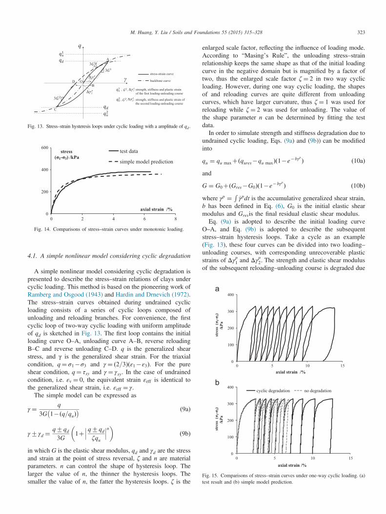
Fig. 13. Stress–strain hysteresis loops under cyclic loading with a amplitude of qd .

0

200

400

600

0 2 4 6 8

stress (σ1-σ3) /kPa

axial strain /%

test data

simple model prediction

Fig. 14. Comparisons of stress–strain curves under monotonic loading.

0

100

200

300

400

0 5 10 15axial strain /%

0

100

200

300

400

0 5 10 15

stre

ss (

σ 1-σ

3)

/kPa

axial strain /%

cyclic degradation no degradation

stre

ss (

σ 1-σ

3)

/kPa

Fig. 15. Comparisons of stress–strain curves under one-way cyclic loading. (a)test result and (b) simple model prediction.

M. Huang, Y. Liu / Soils and Foundations 55 (2015) 315–328 323

4.1. A simple nonlinear model considering cyclic degradation

A simple nonlinear model considering cyclic degradation ispresented to describe the stress–strain relations of clays undercyclic loading. This method is based on the pioneering work ofRamberg and Osgood (1943) and Hardin and Drnevich (1972).The stress–strain curves obtained during undrained cyclicloading consists of a series of cyclic loops composed ofunloading and reloading branches. For convenience, the firstcyclic loop of two-way cyclic loading with uniform amplitudeof qd is sketched in Fig. 13. The first loop contains the initialloading curve O–A, unloading curve A–B, reverse reloadingB–C and reverse unloading C–D. q is the generalized shearstress, and γ is the generalized shear strain. For the triaxialcondition, q¼ σ1�σ3 and γ ¼ ð2=3Þ ε1�ε3ð Þ. For the pureshear condition, q¼ τxy and γ ¼ γxy. In the case of undrainedcondition, i.e. εv ¼ 0, the equivalent strain εeff is identical tothe generalized shear strain, i.e. εeff ¼ γ.

The simple model can be expressed as

γ ¼ q

3G 1�ðq=quÞ� � ð9aÞ

γ7γd ¼q7qd3G

1þ��� q7qd

ζqu

���n� ð9bÞ

in which G is the elastic shear modulus, qd and γd are the stressand strain at the point of stress reversal, ζ and n are materialparameters. n can control the shape of hysteresis loop. Thelarger the value of n, the thinner the hysteresis loops. Thesmaller the value of n, the fatter the hysteresis loops. ζ is the

enlarged scale factor, reflecting the influence of loading mode.According to “Masing’s Rule”, the unloading stress–strainrelationship keeps the same shape as that of the initial loadingcurve in the negative domain but is magnified by a factor oftwo, thus the enlarged scale factor ζ ¼ 2 in two way cyclicloading. However, during one way cyclic loading, the shapesof and reloading curves are quite different from unloadingcurves, which have larger curvature, thus ζ¼ 1 was used forreloading while ζ¼ 2 was used for unloading. The value ofthe shape parameter n can be determined by fitting the testdata.In order to simulate strength and stiffness degradation due to

undrained cyclic loading, Eqs. (9a) and (9b)) can be modifiedinto

qu ¼ qu maxþðqures�qu maxÞð1�e�bγpÞ ð10aÞand

G ¼ G0þðGres�G0Þð1�e�bγpÞ ð10bÞwhere γp ¼ R

_γpdt is the accumulative generalized shear strain,b has been defined in Eq. (6), G0 is the initial elastic shearmodulus and Gresis the final residual elastic shear modulus.Eq. (9a) is adopted to describe the initial loading curve

O–A, and Eq. (9b) is adopted to describe the subsequentstress–strain hysteresis loops. Take a cycle as an example(Fig. 13), these four curves can be divided into two loading–unloading courses, with corresponding unrecoverable plasticstrains of Δγp1 and Δγp2. The strength and elastic shear modulusof the subsequent reloading–unloading course is degraded due

Fig. 16. Pile–soil system under two-way cyclic axial force loading.

M. Huang, Y. Liu / Soils and Foundations 55 (2015) 315–328324

to the accumulative plastic strain γp ðγp ¼ PΔγpi ; i¼ 1; 2; 3;

2N�1; 2NÞ.The simple model was employed to simulate the experi-

mental results of Sangrey et al. (1969). In the triaxialundrained condition, εpv ¼ εp1þεp2þεp3 ¼ 0, consideringγp ¼ ð2=3Þ εp1�εp3

� �and εp2 ¼ εp3, γ

pcan be simply taken as εp1.The enlarged scale factor ζ¼ 2 was adopted for unloading andζ¼ 1 was adopted for reloading, with a shape parameter n is3.6 after adjusting the parameters. Since there is an initialelastic stage in the kinematic hardening model, the initialtangent elastic modulus E in the simple model is much biggerthan the elastic modulus in the kinematic hardening model,which was fixed at 100,000 kPa by adjusting parameter to thetest results for monotonic loading. Other parameters were keptconsistent with those in the kinematic hardening model.Figs. 14 and 15 show the comparisons of stress–strain curvespredicted by the simple model with the test data undermonotonic loading and cyclic loading. The good agreementobtained validates the efficiency of the simple model. Thestress–strain hysteresis loops obtained from the simple modelwith no degradation considered are shown in Fig. 15(b). Aswas the case with the kinematic hardening model, the shape ofthe subsequent stress–strain hysteresis loops remains the samefrom the second loop. The convenience of this simple modelfor practical engineering applications was established by thesecomparisons.

4.2. A nonlinear shear displacement method based on thesimple soil model

A simplified analysis procedure based on the shear dis-placement method for analyzing the behavior of single piles inclay under uniform cyclic axial loading is presented here inorder to reduce the computational burden. The reduction ofshaft stresses caused by cyclic loading is considered using thedegradation of the elastic shear moduli and shaft limitingstress.

Fig. 16 shows a pile–soil system under two-way cyclicaxial force loading with a constant amplitude p0 at the piletop, with N representing the total number of cyclic loading.Because there are two loading–unloading courses in two-waycyclic loading, the total loading–unloading course number is2N. The soil parameters are assumed constant in the sameloading–unloading course. The pile is divided equally into Melements to transfer the cyclic load from pile top to pile base.In the cyclic loading course i (i¼1,2,…,2N), the amplitude ofcyclic shear stress τij around pile element j (j¼1, 2,…,M) canbe calculated by obtaining the pile axial force through theshear displacement method (Cooke, 1974). The pile axialforce can be obtained according to the previous reports(Randolph and Wroth, 1978; Mylonakis and Gazetas,1998), in which the transfer matrix for single pile can beobtained by the method proposed by Mylonakis and Gazetas(1998). The main analysis procedures are outlined briefly inthe following section.

Randolph and Wroth (1978) assumed that the soil surround-ing the pile can be represented by distributed Winkler springs.

The governing equation for pile–soil interaction is givenbelow as

d2Wij zð Þ

dz2� λij

� �2Wi

j zð Þ ¼ 0 ð11Þ

where Wij zð Þ is the axial displacement of pile element j at cyclic

loading course i. The variable λij is

λij ¼ffiffiffiffiffiffiffiffiffiffikij

ApEp

sð12Þ

where Ep and Ap are Young’s modulus and cross-sectional areaof the equivalent solid cylinder pile, respectively. kij is springstiffness of the soil around the pile element j at cyclic loadingcourse i,

kij ¼2π

ln rm=r0� �Gi

j ð13Þ

where Gij is the soil shear modulus around pile element j at

cyclic loading course i, r0 is the pile radius and rm representsthe maximum radius of influence of the pile beyond which theshear stress becomes negligible. rm ¼ χ1χ2L 1�νð Þ, χ1χ2 � 2:5under the condition of homogeneous soil and χ1χ2 � 1:0 forGibson soil (Mylonakis and Gazetas, 1998).As to the stiffness of soil at the pile base Ki

b, it is reasonableto assume that the pile base acts as a rigid circular disk on thesurface of a homogeneous elastic stratum (Randolph andWroth, 1978).

Kib ¼

Pib

Wib

¼ dEib

1�ν2b1þ0:65

d

hb

� ð14Þ

where Eib and νb are Young’s modulus and Poisson’s ratio of

the soil at the pile base level, and d is the diameter of the pile.

0

0.05

0.1

0.15

0.2

0.25

0 50 100 150 200

axia

l dis

plac

emen

t /m

axial force /kN

FEM

simple method

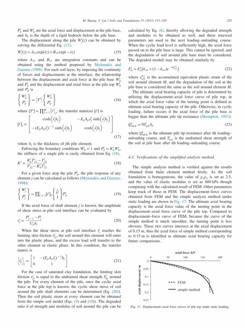
Fig. 17. Displacement–axial force curves of pile top under static loading.

M. Huang, Y. Liu / Soils and Foundations 55 (2015) 315–328 325

Pib and Wi

b are the axial force and displacement at the pile base,and hb is the depth of a rigid bedrock below the pile base.

The displacement along the pile Wij zð Þ can be obtained by

solving the differential Eq. (11),

Wij zð Þ ¼ A11exp λzð ÞþB11exp �λzð Þ ð15Þ

where A11 and B11 are integration constants and can beobtained using the method proposed by Mylonakis andGazetas (1998). For each soil layer, by imposing the continuityof forces and displacements at the interface, the relationshipbetween the displacement and axial force at the pile base Wi

band Pi

b and the displacement and axial force at the pile top Wi0

and Pi0 is

Wib

Pib

( )¼ Ti � Wi

0

Pi0

( )ð16Þ

where ½Ti� ¼∏Mj ¼ 1 ti

�j, the transfer matrices ½ti� is

½ti�j ¼cosh λijhj

� ��EpApλ

ij sinh λijhj

� ��ðEpApλ

ijÞ�1 sinh λijhj

� �cosh λijhj

� �264

375ð17Þ

where hj is the thickness of jth pile element.Enforcing the boundary conditions Wi

0 ¼ 1 and Pib ¼Ki

bWib,

the stiffness of a single pile is easily obtained from Eq. (16),

Ki ¼ KibT

i11�Ti

21

Ti22�Ki

bTi12

ð18Þ

For a given force atop the pile Pi0, the pile response of any

element j can be calculated as follows (Mylonakis and Gazetas,1998):

Wij

Pij

( )¼∏j

k ¼ 1½ti�k1Ki

1

( )Pi0 ð19Þ

If the axial force of shaft element j is known, the amplitudeof shear stress at pile–soil interface can be evaluated by

τij ¼Pij�1�Pi

j

Uphjð20Þ

When the shear stress at pile–soil interface τij reaches thelimiting skin friction τif j, the soil around this element will enterinto the plastic phase, and the excess load will transfer to theother element in elastic phase. In this condition, the transfermatrix is

tif

h ij¼ 1 �ðEpApλ

ij�1hj

0 1

" #ð21Þ

For the case of saturated clay foundation, the limiting skinfriction τif j is equal to the undrained shear strength Siuj aroundthe pile. For every element of the pile, once the cyclic axialforce at the pile top is known, the cyclic shear stress of soilaround the pile shaft elements can be determined (Eq. (20)).Then the soil plastic strain at every element can be obtainedfrom the simple soil model (Eqs. (9) and (10)). The degradedratio δ of strength and modulus of soil around the pile can be

calculated by Eq. (6), thereby allowing the degraded strengthand modulus to be obtained as well, and these renewedparameters are used in the next loading–unloading course.When the cyclic load level is sufficiently high, the axial forcepassed on to the pile base is large. This cannot be ignored, andthe degradation of soil around pile base must be considered.The degraded moduli may be obtained similarly by

Eib ¼ Ei

1½δresþ 1�δresð Þe�bεp;ief f � ð22Þwhere εp;ief f is the accumulated equivalent plastic strain of thesoil around element M, and the degradation of the soil at thepile base is considered the same as the soil around element M.The ultimate axial bearing capacity of pile is determined by

utilizing the displacement–axial force curve of pile top, inwhich the axial force value of the turning point is defined asultimate axial bearing capacity of the pile. Otherwise, in cyclicloading, failure occurs if the axial force of the pile base isbigger than the ultimate pile tip resistance (Skempton, 1951):

Qiult;b ¼ 9Siu;bAp ð23Þ

where Qiult;b is the ultimate pile tip resistance after ith loading–

unloading course, and Siu;b is the undrained shear strength ofthe soil at pile base after ith loading–unloading course.

4.3. Verifications of the simplified analysis method

The simple analysis method is verified against the resultsobtained from finite element method firstly. As the soilfoundation is homogeneous, the value of χ1χ2 is set as 2.5,and the value of elastic modulus is set as 600 kPa thoughcomparing with the calculated result of FEM. Other parameterskeep track of those in FEM. The displacement–force curvesobtained from FEM and the simple analysis method understatic loading are shown in Fig. 17. The ultimate axial bearingcapacity is the axial force value of the turning point in thedisplacement–axial force curve of the pile top. Compared todisplacement–force curve of FEM, because the curve of thesimple method is much smoother, the turning point is lessobvious. These two curves intersect at the axial displacementof 0.15 m, thus the axial force of simple method correspondingto 0.15 m is identified as ultimate axial bearing capacity forfuture comparisons.

Fig. 18. Comparisons of stress–strain curves between the simple modeland FEM at different Qc=Qus. (a) Qc=Qus¼0.2, (b) Qc=Qus¼0.4 and(c) Qc=Qus¼0.6.

0.5

1

1.5

0 0.2 0.4 0.6 0.8

Quc

/Qus

Qc /Qus

after 10 cycles simple method

after 50 cycles simple method

after 100 cycles simple method

after 10 cycles FEM

after 50 cycles FEM

after 100 cycles FEM

Fig. 19. The ultimate bearing capacity of single pile after cyclic loading (FEMand the simple method).

0.6

0.8

1

1.2

1 10 100 1000

Quc

/Qus

No. of cycles

Qc/Qus

0.1 0.2 0.4 0.75

failure

Fig. 20. The ultimate bearing capacity of single pile after long term cyclicloading by the simple method.

M. Huang, Y. Liu / Soils and Foundations 55 (2015) 315–328326

As this is two-way cyclic loading, the enlarged scale factoradopted was ζ¼ 2. In the absence of relevant tests data for thesimple soil model, the shape parameter n is set as 1.5 byadjusting parameters to compare with stress–strain loops of thefirst cycle obtained from FEM at different cyclic load levels(Fig. 18). Although the shape of stress–strain loops obtainedfrom these two methods are very close, discrepancies stillexist. The stress–strain loops of simple method vary moresignificantly than that of FEM, e.g., the loop of simple methodwith current parameters is thinner than that of FEM atQc=Qus ¼ 0:4 but fatter than that of FEM at Qc=Qus ¼ 0:6.

Comparisons of ultimate bearing capacities after differentnumber of cycles and different cyclic load levels calculated bythe two methods are shown in Fig. 19. The agreement isremarkably good, and the faster development of ultimatebearing capacity degradation at higher cyclic load levels isclear for both two methods. However, since there is no initialelastic stage in the simple nonlinear soil model, unlike thekinematic hardening model, cyclic degradation occurs at verylow cyclic load levels. This discrepancy can be ignored whenthe number of cyclic loading is small. Theoretical resultsobtained from the simplified analysis procedure reveal similarvaluable information about the effect of previous cyclicloading on the ultimate load capacity of single piles.

In addition to this, this method has the advantage of computa-tional speed for long-term cyclic loading. The forecast of longterm cyclic loading calculated by the simple method is shownin Fig. 20. Although the very little degradation occurred forlow cyclic load levels after a few cycles (Qc=Qus ¼ 0:1, No. ofcycles¼10), the accumulative effect after long-term cyclicloading is obvious (Qc=Qus ¼ 0:1, No. of cycles¼1000). Itshould be noted that this degradation was not clear in theresults from FEM. A comparison of the curves ofQc=Qus ¼ 0:2 and Qc=Qus ¼ 0:4, the steady state of degrada-tion will be achieved earlier at higher cyclic load level. Failureoccurs after 11 cycles at Qc=Qus ¼ 0:75, which means at thattime the cyclic shear stress at pile side has exceeded theresidual strength ratio of the soil.The simplified procedure was employed to simulate the

model tests by Poulos (1979). The enlarged scale factor ζ¼ 2was employed, as it was for two-way cyclic loading. In theabsence of relevant test data for the simple soil model, theshape parameter n is set as 2.5 by comparing the first stress–strain loops with that in FEM (Fig. 21). The value of χ1χ2 isset as 1.1 and the elastic modulus is set as 12 MPa afterreferring to the static loading results calculated by FEM. Theother parameters keep track of those in FEM. Good agreementbetween the simplified procedure and the experiment are alsoachieved in the degraded ultimate bearing capacity after acyclic loading of N¼100 and N¼1000 (Fig. 22).

Fig. 21. Comparisons stress–strain curves of soil around pile top between ofthe simple model and FEM for Poulos’ model tests. (a) Qc=Qus¼0.6 and(b) Qc=Qus¼0.9.

0

0.5

1

0 0.2 0.4 0.6

Quc

/Qus

Qc/Qus

model test (Poulos,1979) N=100

FEM N=100

simple method N=100

model test (Poulos,1979) N=1000

simple method N=1000

Fig. 22. The ultimate bearing capacity of single pile after cyclic loading(simple method, FEM and model test).

M. Huang, Y. Liu / Soils and Foundations 55 (2015) 315–328 327

With fewer parameters and higher computational speed, thesimple analysis method based on the simple soil model is afriendly engineering method for predicting the axial capacitydegradation of single piles under long-term cyclic loading.However, the selection of the parameters is very important andany small deviation from true value is likely to result insignificant error after a large number of load repetitions.Therefore, static and dynamic triaxial tests are needed todetermine the soil parameters such as the shear modulus,undrained strength, shape parameter, and degraded parametersδres and b before engineering application.

5. Conclusions

A kinematic hardening constitutive model was developedfor cyclic degradation to analyze the cyclic axial response ofsingle piles in saturated clay using commercially availablefinite element software. A more simplified analytical approach

based on a simple nonlinear model for cyclic degradation wassuggested in order to reduce the computation burden. Both ofthese soil models were validated against dynamic triaxial testresults (Sangrey et al., 1969), and both of these anaylsismethods were verified against the 1 g model tests by Poulos(1979).

�

A cyclic degradation model for the strength of saturatedclay was presented. This model is imported into thesimplified kinematic hardening model provided in ABA-QUS. Two modifications were made by user subroutine.The degradation of soil stiffness was complemented, andthe size of the yield surface was set to remain unchangedunder monotonic loading. This model was shown capableof predicting different behaviors of clay with increasingcyclic stress levels, including the elastic state, the elasto-plastic steady state and the elastoplastic failure state. In theFEM based on the kinematic hardening model, the pile–soilsystem remains elastic without any degradation at lowcyclic load levels. The ultimate axial bearing capacity ofpile foundation degrades after cyclic loading, with degrada-tion developing rapidly at higher cyclic load levels or aftermore loading cycles.

�

In the simple nonlinear model, degradations for strengthand stiffness of saturated clay were also considered.Because the simple model cannot describe the elasticstress–strain relations at low stress levels, discrepancieswere apparent between cyclic degradations obtained fromthe FEM and the simple method at low cyclic load levels.Nevertheless, results calculated by this simple analysis atrelatively high cyclic load levels were consistent with thoseof numerical simulation.

Unlike conventional theories which empirically expressdegradation factors as a function of the number of loadingcycles, both the FEM and the simple method are based on theconstitutive models of soil. This alone makes these modelsmore consistent with theory and more reliable. Considering thecomplexity and diversity of soils, tests are necessary for getingexact parameters of the models. Still more research is in greatneed. The simple method has potential to serve as a useful toolin engineering design in the future.

Acknowledgement

This work was financially supported by the National BasicProgram of China (973 Program, Grant no. 2013CB036304),the National Natural Science Foundation of China (Grant nos.51378392 and 41362016). These supports are gratefullyacknowledged.

References

Anastasopoulos, I., Gelagoti, F., Kourkoulis, R., et al., 2011. Simplifiedconstitutive model for simulation of cyclic response of shallow

M. Huang, Y. Liu / Soils and Foundations 55 (2015) 315–328328

foundations: validation against laboratory tests. J. Geotech. Eng. ASCE137, 1154–1168.

Andersen, K.H., Pool, J.H., Brown, S.F., et al., 1980. Cyclic and staticlaboratory tests on Drammen clay. J. Geotech. Eng. ASCE 106 (5), 499–529.

Armstrong, P.J., Frederick, C.O., A mathematical Representation of theMultiaxial Bauschinger Effect. CEGB Rep. No. RD/B/N 731, 1966.

Carter, J.P., Booker, J.R., Wroth, C.P., 1982. A critical state soil modelfor cyclic loading. In: Panda, G.N., Zienkiewicz, O.C. (Eds.), SoilMechanics—Transient and Cyclic Loads. John Wiley & Sons Ltd., NewYork, pp. 219–252.

Cooke, R.W. The settlement of friction pile foundations. In: Proceedings of theConference on Tall Buildings, Kuala Lumpur, Malaysia, 1974.

Giannakos, S., Gerolymos, N., Gazetas, G., 2012. Cyclic lateral response ofpiles in dry sand: finite element modeling and validation. Comput.Geotech. 44, 116–131.

Hardin, B.O., Drnevich, V.P., 1972. Shear modulus and damping in soils:designequations and curves. J. Soil Mech. Found. Eng. Div. ASCE 98 (7), 667–692.

Huang, M.S., Li, S., 2010. Degradation of stiffness and strength of offshoresaturated soft clay under long-term cyclic loading. Chin. J. Geotech. Eng.32 (10), 1491–1498 in Chinese.

Hyodo, M., Yamamoto, Y., Sugiyama, M., 1994. Undrained cyclic shearbehavior of normally consolidated clay subjected to initial static shearstress. Soils Found. 34 (4), 1–11.

Jardine, R.J., Standing, J.R., 2012. Field axial cyclic loading experiments onpiles driven in sand. Soils Found. 52 (4), 723–736.

Lee, C.Y., 1993. Cyclic response of axial loaded pile groups. J. Geotech. Eng.ASCE 119 (9), 1399–1412.

Lemaitre, J., Chaboche, J.L., 1990. Mechanics of Solid Materials. CambridgeUniversity Press, Cambridge, UK.

Lombardi, D., Bhattacharya, S., Wood, D.M., 2013. Dynamic soil–structureinteraction of monopole supported wind turbines in cohesive soil. SoilDyn. Earthquake Eng. 49, 165–180.

Lesny, K., Hinz, P., 2009. Design of monopile foundations for offshore wind energyconverters GSP No. 185. Contemp. Topics Deep Found. ASCE, 512–519.

Mróz, Z., Norris, V.A., Zienkiewicz, O.C., 1981. An anisotropic, criticalstate model for soils subject to cyclic loading. Géotechnique 31 (4),451–469.

Mylonakis, G., Gazetas, G., 1998. Settlement and additional internal forces ofgrouped piles in layered soil. Geotechnique 48 (1), 55–72.

Poulos, H. G. ,Development of an analysis for cyclic axial loading of piles. In:Proceedings of Third International Conference on Numerical Methods inGeomechanics, Vol.4, Aachen, Germany, A. Balkema, Rotterdam, 1979,pp. 1513-1530.

Poulos, H.G., 1981. Cyclic axial response of single pile. J. Geotech. Eng.ASCE 107 (1), 41–58.

Poulos, H.G., 1987. Analysis of residual stress effects in piles. J. Geotech. Eng.ASCE 113 (3), 216–229.

Poulos, H.G., 1988. Cyclic stability diagram for axially loaded piles. J.Geotech. Eng. ASCE 114 (8), 877–895.

Prévost, J.H., 1977. Mathematical modeling of monotonic and cyclic undrainedclay behavior. Int. J. Numer. Anal. Methods Geomech. 1, 195–216.

Ramberg, W., Osgood, W.R., 1943. Description of stress–strain curves bythree parameters Technical Note 902. National Advisory Committee forAeronautics, Washington, D.C.

Randolph, M.F., Wroth, C.P., 1978. Analysis of deformation of verticallyloaded piles. J. Geotech. Eng. ASCE 104 (12), 1465–1488.

Sangrey, D.A., Henkel, D.J., Esrig, M.I., 1969. The effective stressresponse of a saturated clay soil to repeated loading. Can. Geotech. J. 6,241–252.

Skempton, A.W., The bearing capacity of clays. In: Proceedings of BuildingResearch Congress, vol. 1, 1951, pp. 180–189.

Soroush, A., Soltani-Jigheh, H., 2009. Pre- and post-cyclic behavior if mixedclayed soils. Can. Geotech. J. 46, 115–128.

Tsuha, C.H.C., Foray, P.Y., Jardine, R.J., et al., 2012. Behaviour ofdisplacement piles in sand under cyclic axial loading. Soils Found. 52 (3),393–410.

Zergoun, M., Vaid, Y.P., 1994. Effective stress response of clay to undrainedcyclic loading. Can. Geotech. J. 31, 714–727.