Embed Size (px)
Citation preview

Calculus 1 to 4 (2004–2006)
Axel Schuler
January 3, 2007

2

Contents
1 Real and Complex Numbers 11Basics . . . . . . . . . . . . . . . . . . . . . . . . . . . . . . . . . . . . . . . . . . 11
Notations . . . . . . . . . . . . . . . . . . . . . . . . . . . . . . . . . . . . . 11Sums and Products . . . . . . . . . . . . . . . . . . . . . . . . . . . . . . . . 12Mathematical Induction . . . . . . . . . . . . . . . . . . . . . . . . . . . . . .12Binomial Coefficients . . . . . . . . . . . . . . . . . . . . . . . . . . . . . . . 13
1.1 Real Numbers . . . . . . . . . . . . . . . . . . . . . . . . . . . . . . . . . . . 151.1.1 Ordered Sets . . . . . . . . . . . . . . . . . . . . . . . . . . . . . . . 151.1.2 Fields . . . . . . . . . . . . . . . . . . . . . . . . . . . . . . . . . . . 171.1.3 Ordered Fields . . . . . . . . . . . . . . . . . . . . . . . . . . . . . . 191.1.4 Embedding of natural numbers into the real numbers . . .. . . . . . . 201.1.5 The completeness ofR . . . . . . . . . . . . . . . . . . . . . . . . . . 211.1.6 The Absolute Value . . . . . . . . . . . . . . . . . . . . . . . . . . . . 221.1.7 Supremum and Infimum revisited . . . . . . . . . . . . . . . . . . . .231.1.8 Powers of real numbers . . . . . . . . . . . . . . . . . . . . . . . . . . 241.1.9 Logarithms . . . . . . . . . . . . . . . . . . . . . . . . . . . . . . . . 26
1.2 Complex numbers . . . . . . . . . . . . . . . . . . . . . . . . . . . . . . . . . 291.2.1 The Complex Plane and the Polar form . . . . . . . . . . . . . . . .. 311.2.2 Roots of Complex Numbers . . . . . . . . . . . . . . . . . . . . . . . 33
1.3 Inequalities . . . . . . . . . . . . . . . . . . . . . . . . . . . . . . . . . . . .341.3.1 Monotony of the Power and Exponential Functions . . . . .. . . . . . 341.3.2 The Arithmetic-Geometric mean inequality . . . . . . . . .. . . . . . 341.3.3 The Cauchy–Schwarz Inequality . . . . . . . . . . . . . . . . . . .. . 35
1.4 Appendix A . . . . . . . . . . . . . . . . . . . . . . . . . . . . . . . . . . . . 36
2 Sequences and Series 432.1 Convergent Sequences . . . . . . . . . . . . . . . . . . . . . . . . . . . . .. 43
2.1.1 Algebraic operations with sequences . . . . . . . . . . . . . .. . . . . 462.1.2 Some special sequences . . . . . . . . . . . . . . . . . . . . . . . . . 492.1.3 Monotonic Sequences . . . . . . . . . . . . . . . . . . . . . . . . . . 502.1.4 Subsequences . . . . . . . . . . . . . . . . . . . . . . . . . . . . . . . 51
2.2 Cauchy Sequences . . . . . . . . . . . . . . . . . . . . . . . . . . . . . . . . 552.3 Series . . . . . . . . . . . . . . . . . . . . . . . . . . . . . . . . . . . . . . . 57
3

4 CONTENTS
2.3.1 Properties of Convergent Series . . . . . . . . . . . . . . . . . .. . . 572.3.2 Operations with Convergent Series . . . . . . . . . . . . . . . .. . . . 592.3.3 Series of Nonnegative Numbers . . . . . . . . . . . . . . . . . . . .. 592.3.4 The Numbere . . . . . . . . . . . . . . . . . . . . . . . . . . . . . . 612.3.5 The Root and the Ratio Tests . . . . . . . . . . . . . . . . . . . . . . .632.3.6 Absolute Convergence . . . . . . . . . . . . . . . . . . . . . . . . . . 652.3.7 Decimal Expansion of Real Numbers . . . . . . . . . . . . . . . . .. 662.3.8 Complex Sequences and Series . . . . . . . . . . . . . . . . . . . . .672.3.9 Power Series . . . . . . . . . . . . . . . . . . . . . . . . . . . . . . . 682.3.10 Rearrangements . . . . . . . . . . . . . . . . . . . . . . . . . . . . . . 692.3.11 Products of Series . . . . . . . . . . . . . . . . . . . . . . . . . . . . 72
3 Functions and Continuity 753.1 Limits of a Function . . . . . . . . . . . . . . . . . . . . . . . . . . . . . . .. 76
3.1.1 One-sided Limits, Infinite Limits, and Limits at Infinity . . . . . . . . . 773.2 Continuous Functions . . . . . . . . . . . . . . . . . . . . . . . . . . . . .. . 80
3.2.1 The Intermediate Value Theorem . . . . . . . . . . . . . . . . . . .. . 813.2.2 Continuous Functions on Bounded and Closed Intervals—The Theorem about Maximum and Minimum
3.3 Uniform Continuity . . . . . . . . . . . . . . . . . . . . . . . . . . . . . . .. 833.4 Monotonic Functions . . . . . . . . . . . . . . . . . . . . . . . . . . . . . .. 853.5 Exponential, Trigonometric, and Hyperbolic Functionsand their Inverses . . . 86
3.5.1 Exponential and Logarithm Functions . . . . . . . . . . . . . .. . . . 863.5.2 Trigonometric Functions and their Inverses . . . . . . . .. . . . . . . 893.5.3 Hyperbolic Functions and their Inverses . . . . . . . . . . .. . . . . . 94
3.6 Appendix B . . . . . . . . . . . . . . . . . . . . . . . . . . . . . . . . . . . . 953.6.1 Monotonic Functions have One-Sided Limits . . . . . . . . .. . . . . 953.6.2 Proofs forsin x andcosx inequalities . . . . . . . . . . . . . . . . . . 963.6.3 Estimates forπ . . . . . . . . . . . . . . . . . . . . . . . . . . . . . . 97
4 Differentiation 1014.1 The Derivative of a Function . . . . . . . . . . . . . . . . . . . . . . . .. . . 1014.2 The Derivatives of Elementary Functions . . . . . . . . . . . . .. . . . . . . 107
4.2.1 Derivatives of Higher Order . . . . . . . . . . . . . . . . . . . . . .. 1084.3 Local Extrema and the Mean Value Theorem . . . . . . . . . . . . . .. . . . 108
4.3.1 Local Extrema and Convexity . . . . . . . . . . . . . . . . . . . . . .1114.4 L’Hospital’s Rule . . . . . . . . . . . . . . . . . . . . . . . . . . . . . . . .. 1124.5 Taylor’s Theorem . . . . . . . . . . . . . . . . . . . . . . . . . . . . . . . . .113
4.5.1 Examples of Taylor Series . . . . . . . . . . . . . . . . . . . . . . . .1154.6 Appendix C . . . . . . . . . . . . . . . . . . . . . . . . . . . . . . . . . . . . 117
5 Integration 1195.1 The Riemann–Stieltjes Integral . . . . . . . . . . . . . . . . . . . .. . . . . . 119
5.1.1 Properties of the Integral . . . . . . . . . . . . . . . . . . . . . . .. . 126

CONTENTS 5
5.2 Integration and Differentiation . . . . . . . . . . . . . . . . . . .. . . . . . . 1325.2.1 Table of Antiderivatives . . . . . . . . . . . . . . . . . . . . . . . .. 1345.2.2 Integration Rules . . . . . . . . . . . . . . . . . . . . . . . . . . . . . 1355.2.3 Integration of Rational Functions . . . . . . . . . . . . . . . .. . . . 1385.2.4 Partial Fraction Decomposition . . . . . . . . . . . . . . . . . .. . . 1405.2.5 Other Classes of Elementary Integrable Functions . . .. . . . . . . . . 141
5.3 Improper Integrals . . . . . . . . . . . . . . . . . . . . . . . . . . . . . . .. 1435.3.1 Integrals on unbounded intervals . . . . . . . . . . . . . . . . .. . . . 1435.3.2 Integrals of Unbounded Functions . . . . . . . . . . . . . . . . .. . . 1465.3.3 The Gamma function . . . . . . . . . . . . . . . . . . . . . . . . . . . 147
5.4 Integration of Vector-Valued Functions . . . . . . . . . . . . .. . . . . . . . . 1485.5 Inequalities . . . . . . . . . . . . . . . . . . . . . . . . . . . . . . . . . . . .1505.6 Appendix D . . . . . . . . . . . . . . . . . . . . . . . . . . . . . . . . . . . . 151
5.6.1 More on the Gamma Function . . . . . . . . . . . . . . . . . . . . . . 152
6 Sequences of Functions and Basic Topology 1576.1 Discussion of the Main Problem . . . . . . . . . . . . . . . . . . . . . .. . . 1576.2 Uniform Convergence . . . . . . . . . . . . . . . . . . . . . . . . . . . . . .. 158
6.2.1 Definitions and Example . . . . . . . . . . . . . . . . . . . . . . . . . 1586.2.2 Uniform Convergence and Continuity . . . . . . . . . . . . . . .. . . 1626.2.3 Uniform Convergence and Integration . . . . . . . . . . . . . .. . . . 1636.2.4 Uniform Convergence and Differentiation . . . . . . . . . .. . . . . . 166
6.3 Fourier Series . . . . . . . . . . . . . . . . . . . . . . . . . . . . . . . . . . .1686.3.1 An Inner Product on the Periodic Functions . . . . . . . . . .. . . . . 171
6.4 Basic Topology . . . . . . . . . . . . . . . . . . . . . . . . . . . . . . . . . . 1776.4.1 Finite, Countable, and Uncountable Sets . . . . . . . . . . .. . . . . . 1776.4.2 Metric Spaces and Normed Spaces . . . . . . . . . . . . . . . . . . .. 1786.4.3 Open and Closed Sets . . . . . . . . . . . . . . . . . . . . . . . . . . 1806.4.4 Limits and Continuity . . . . . . . . . . . . . . . . . . . . . . . . . . 1826.4.5 Comleteness and Compactness . . . . . . . . . . . . . . . . . . . . .. 1856.4.6 Continuous Functions inRk . . . . . . . . . . . . . . . . . . . . . . . 187
6.5 Appendix E . . . . . . . . . . . . . . . . . . . . . . . . . . . . . . . . . . . . 188
7 Calculus of Functions of Several Variables 1937.1 Partial Derivatives . . . . . . . . . . . . . . . . . . . . . . . . . . . . . .. . . 194
7.1.1 Higher Partial Derivatives . . . . . . . . . . . . . . . . . . . . . .. . 1977.1.2 The Laplacian . . . . . . . . . . . . . . . . . . . . . . . . . . . . . . . 199
7.2 Total Differentiation . . . . . . . . . . . . . . . . . . . . . . . . . . . .. . . . 1997.2.1 Basic Theorems . . . . . . . . . . . . . . . . . . . . . . . . . . . . . . 202
7.3 Taylor’s Formula . . . . . . . . . . . . . . . . . . . . . . . . . . . . . . . . .2067.3.1 Directional Derivatives . . . . . . . . . . . . . . . . . . . . . . . .. . 2067.3.2 Taylor’s Formula . . . . . . . . . . . . . . . . . . . . . . . . . . . . . 208
7.4 Extrema of Functions of Several Variables . . . . . . . . . . . .. . . . . . . . 211

6 CONTENTS
7.5 The Inverse Mapping Theorem . . . . . . . . . . . . . . . . . . . . . . . .. . 2167.6 The Implicit Function Theorem . . . . . . . . . . . . . . . . . . . . . .. . . . 2197.7 Lagrange Multiplier Rule . . . . . . . . . . . . . . . . . . . . . . . . . .. . . 2237.8 Integrals depending on Parameters . . . . . . . . . . . . . . . . . .. . . . . . 225
7.8.1 Continuity ofI(y) . . . . . . . . . . . . . . . . . . . . . . . . . . . . 2257.8.2 Differentiation of Integrals . . . . . . . . . . . . . . . . . . . .. . . . 2257.8.3 Improper Integrals with Parameters . . . . . . . . . . . . . . .. . . . 227
7.9 Appendix . . . . . . . . . . . . . . . . . . . . . . . . . . . . . . . . . . . . . 230
8 Curves and Line Integrals 2318.1 Rectifiable Curves . . . . . . . . . . . . . . . . . . . . . . . . . . . . . . . .. 231
8.1.1 Curves inRk . . . . . . . . . . . . . . . . . . . . . . . . . . . . . . . 2318.1.2 Rectifiable Curves . . . . . . . . . . . . . . . . . . . . . . . . . . . . 233
8.2 Line Integrals . . . . . . . . . . . . . . . . . . . . . . . . . . . . . . . . . . .2368.2.1 Path Independence . . . . . . . . . . . . . . . . . . . . . . . . . . . . 239
9 Integration of Functions of Several Variables 2459.1 Basic Definition . . . . . . . . . . . . . . . . . . . . . . . . . . . . . . . . . .245
9.1.1 Properties of the Riemann Integral . . . . . . . . . . . . . . . .. . . . 2479.2 Integrable Functions . . . . . . . . . . . . . . . . . . . . . . . . . . . . .. . 248
9.2.1 Integration over More General Sets . . . . . . . . . . . . . . . .. . . 2499.2.2 Fubini’s Theorem and Iterated Integrals . . . . . . . . . . .. . . . . . 250
9.3 Change of Variable . . . . . . . . . . . . . . . . . . . . . . . . . . . . . . . .2539.4 Appendix . . . . . . . . . . . . . . . . . . . . . . . . . . . . . . . . . . . . . 257
10 Surface Integrals 25910.1 Surfaces inR3 . . . . . . . . . . . . . . . . . . . . . . . . . . . . . . . . . . . 259
10.1.1 The Area of a Surface . . . . . . . . . . . . . . . . . . . . . . . . . . 26110.2 Scalar Surface Integrals . . . . . . . . . . . . . . . . . . . . . . . . .. . . . . 262
10.2.1 Other Forms fordS . . . . . . . . . . . . . . . . . . . . . . . . . . . 26210.2.2 Physical Application . . . . . . . . . . . . . . . . . . . . . . . . . .. 264
10.3 Surface Integrals . . . . . . . . . . . . . . . . . . . . . . . . . . . . . . .. . 26410.3.1 Orientation . . . . . . . . . . . . . . . . . . . . . . . . . . . . . . . . 264
10.4 Gauß’ Divergence Theorem . . . . . . . . . . . . . . . . . . . . . . . . .. . . 26810.5 Stokes’ Theorem . . . . . . . . . . . . . . . . . . . . . . . . . . . . . . . . .272
10.5.1 Green’s Theorem . . . . . . . . . . . . . . . . . . . . . . . . . . . . . 27210.5.2 Stokes’ Theorem . . . . . . . . . . . . . . . . . . . . . . . . . . . . . 27410.5.3 Vector Potential and the Inverse Problem of Vector Analysis . . . . . . 276
11 Differential Forms onRn 27911.1 The Exterior AlgebraΛ(Rn) . . . . . . . . . . . . . . . . . . . . . . . . . . . 279
11.1.1 The Dual Vector SpaceV ∗ . . . . . . . . . . . . . . . . . . . . . . . . 27911.1.2 The Pull-Back ofk-forms . . . . . . . . . . . . . . . . . . . . . . . . 28411.1.3 Orientation ofRn . . . . . . . . . . . . . . . . . . . . . . . . . . . . . 285
CONTENTS 7
11.2 Differential Forms . . . . . . . . . . . . . . . . . . . . . . . . . . . . . .. . . 28511.2.1 Definition . . . . . . . . . . . . . . . . . . . . . . . . . . . . . . . . . 28511.2.2 Differentiation . . . . . . . . . . . . . . . . . . . . . . . . . . . . . .28611.2.3 Pull-Back . . . . . . . . . . . . . . . . . . . . . . . . . . . . . . . . . 28811.2.4 Closed and Exact Forms . . . . . . . . . . . . . . . . . . . . . . . . . 291
11.3 Stokes’ Theorem . . . . . . . . . . . . . . . . . . . . . . . . . . . . . . . . .29311.3.1 Singular Cubes, Singular Chains, and the Boundary Operator . . . . . 29311.3.2 Integration . . . . . . . . . . . . . . . . . . . . . . . . . . . . . . . . 29511.3.3 Stokes’ Theorem . . . . . . . . . . . . . . . . . . . . . . . . . . . . . 29611.3.4 Special Cases . . . . . . . . . . . . . . . . . . . . . . . . . . . . . . 29811.3.5 Applications . . . . . . . . . . . . . . . . . . . . . . . . . . . . . . . 299
12 Measure Theory and Integration 30512.1 Measure Theory . . . . . . . . . . . . . . . . . . . . . . . . . . . . . . . . . .305
12.1.1 Algebras,σ-algebras, and Borel Sets . . . . . . . . . . . . . . . . . . . 30612.1.2 Additive Functions and Measures . . . . . . . . . . . . . . . . .. . . 30812.1.3 Extension of Countably Additive Functions . . . . . . . .. . . . . . . 31312.1.4 The Lebesgue Measure onRn . . . . . . . . . . . . . . . . . . . . . . 314
12.2 Measurable Functions . . . . . . . . . . . . . . . . . . . . . . . . . . . .. . . 31612.3 The Lebesgue Integral . . . . . . . . . . . . . . . . . . . . . . . . . . . .. . 318
12.3.1 Simple Functions . . . . . . . . . . . . . . . . . . . . . . . . . . . . . 31812.3.2 Positive Measurable Functions . . . . . . . . . . . . . . . . . .. . . 319
12.4 Some Theorems on Lebesgue Integrals . . . . . . . . . . . . . . . .. . . . . . 32212.4.1 The Role Played by Measure Zero Sets . . . . . . . . . . . . . . .. . 32212.4.2 The spaceLp(X,µ) . . . . . . . . . . . . . . . . . . . . . . . . . . . . 32412.4.3 The Monotone Convergence Theorem . . . . . . . . . . . . . . . .. . 32512.4.4 The Dominated Convergence Theorem . . . . . . . . . . . . . . .. . 32612.4.5 Application of Lebesgue’s Theorem to Parametric Integrals . . . . . . . 32712.4.6 The Riemann and the Lebesgue Integrals . . . . . . . . . . . .. . . . 32912.4.7 Appendix: Fubini’s Theorem . . . . . . . . . . . . . . . . . . . . .. . 329
13 Hilbert Space 33113.1 The Geometry of the Hilbert Space . . . . . . . . . . . . . . . . . . .. . . . . 331
13.1.1 Unitary Spaces . . . . . . . . . . . . . . . . . . . . . . . . . . . . . . 33113.1.2 Norm and Inner product . . . . . . . . . . . . . . . . . . . . . . . . . 33413.1.3 Two Theorems of F. Riesz . . . . . . . . . . . . . . . . . . . . . . . . 33513.1.4 Orthogonal Sets and Fourier Expansion . . . . . . . . . . . .. . . . . 33913.1.5 Appendix . . . . . . . . . . . . . . . . . . . . . . . . . . . . . . . . . 343
13.2 Bounded Linear Operators in Hilbert Spaces . . . . . . . . . .. . . . . . . . . 34413.2.1 Bounded Linear Operators . . . . . . . . . . . . . . . . . . . . . . .. 34413.2.2 The Adjoint Operator . . . . . . . . . . . . . . . . . . . . . . . . . . .34713.2.3 Classes of Bounded Linear Operators . . . . . . . . . . . . . .. . . . 34913.2.4 Orthogonal Projections . . . . . . . . . . . . . . . . . . . . . . . .. . 351

8 CONTENTS
13.2.5 Spectrum and Resolvent . . . . . . . . . . . . . . . . . . . . . . . . .35313.2.6 The Spectrum of Self-Adjoint Operators . . . . . . . . . . .. . . . . . 357
14 Complex Analysis 36314.1 Holomorphic Functions . . . . . . . . . . . . . . . . . . . . . . . . . . .. . . 363
14.1.1 Complex Differentiation . . . . . . . . . . . . . . . . . . . . . . .. . 36314.1.2 Power Series . . . . . . . . . . . . . . . . . . . . . . . . . . . . . . . 36514.1.3 Cauchy–Riemann Equations . . . . . . . . . . . . . . . . . . . . . .. 366
14.2 Cauchy’s Integral Formula . . . . . . . . . . . . . . . . . . . . . . . .. . . . 36914.2.1 Integration . . . . . . . . . . . . . . . . . . . . . . . . . . . . . . . . 36914.2.2 Cauchy’s Theorem . . . . . . . . . . . . . . . . . . . . . . . . . . . . 37114.2.3 Cauchy’s Integral Formula . . . . . . . . . . . . . . . . . . . . . .. . 37314.2.4 Applications of the Coefficient Formula . . . . . . . . . . .. . . . . . 37714.2.5 Power Series . . . . . . . . . . . . . . . . . . . . . . . . . . . . . . . 380
14.3 Local Properties of Holomorphic Functions . . . . . . . . . .. . . . . . . . . 38314.4 Singularities . . . . . . . . . . . . . . . . . . . . . . . . . . . . . . . . . .. . 385
14.4.1 Classification of Singularities . . . . . . . . . . . . . . . . .. . . . . 38614.4.2 Laurent Series . . . . . . . . . . . . . . . . . . . . . . . . . . . . . . 387
14.5 Residues . . . . . . . . . . . . . . . . . . . . . . . . . . . . . . . . . . . . . . 39214.5.1 Calculating Residues . . . . . . . . . . . . . . . . . . . . . . . . . .. 394
14.6 Real Integrals . . . . . . . . . . . . . . . . . . . . . . . . . . . . . . . . . .. 39514.6.1 Rational Functions in Sine and Cosine . . . . . . . . . . . . .. . . . . 39514.6.2 Integrals of the form
∫∞−∞ f(x) dx . . . . . . . . . . . . . . . . . . . . 396
15 Partial Differential Equations I — an Introduction 40115.1 Classification of PDE . . . . . . . . . . . . . . . . . . . . . . . . . . . . .. . 401
15.1.1 Introduction . . . . . . . . . . . . . . . . . . . . . . . . . . . . . . . . 40115.1.2 Examples . . . . . . . . . . . . . . . . . . . . . . . . . . . . . . . . . 402
15.2 First Order PDE — The Method of Characteristics . . . . . . .. . . . . . . . 40515.3 Classification of Semi-Linear Second-Order PDEs . . . . .. . . . . . . . . . . 408
15.3.1 Quadratic Forms . . . . . . . . . . . . . . . . . . . . . . . . . . . . . 40815.3.2 Elliptic, Parabolic and Hyperbolic . . . . . . . . . . . . . .. . . . . . 40815.3.3 Change of Coordinates . . . . . . . . . . . . . . . . . . . . . . . . . .40915.3.4 Characteristics . . . . . . . . . . . . . . . . . . . . . . . . . . . . . .41115.3.5 The Vibrating String . . . . . . . . . . . . . . . . . . . . . . . . . . .414
16 Distributions 41716.1 Introduction — Test Functions and Distributions . . . . .. . . . . . . . . . . . 417
16.1.1 Motivation . . . . . . . . . . . . . . . . . . . . . . . . . . . . . . . . 41716.1.2 Test FunctionsD(Rn) andD(Ω) . . . . . . . . . . . . . . . . . . . . 418
16.2 The DistributionsD′(Rn) . . . . . . . . . . . . . . . . . . . . . . . . . . . . . 42216.2.1 Regular Distributions . . . . . . . . . . . . . . . . . . . . . . . . .. . 42216.2.2 Other Examples of Distributions . . . . . . . . . . . . . . . . .. . . . 424
CONTENTS 9
16.2.3 Convergence and Limits of Distributions . . . . . . . . . .. . . . . . 42516.2.4 The distributionP 1
x. . . . . . . . . . . . . . . . . . . . . . . . . . . 426
16.2.5 Operation with Distributions . . . . . . . . . . . . . . . . . . .. . . . 42716.3 Tensor Product and Convolution Product . . . . . . . . . . . . .. . . . . . . . 433
16.3.1 The Support of a Distribution . . . . . . . . . . . . . . . . . . . .. . 43316.3.2 Tensor Products . . . . . . . . . . . . . . . . . . . . . . . . . . . . . . 43316.3.3 Convolution Product . . . . . . . . . . . . . . . . . . . . . . . . . . .43416.3.4 Linear Change of Variables . . . . . . . . . . . . . . . . . . . . . .. . 43716.3.5 Fundamental Solutions . . . . . . . . . . . . . . . . . . . . . . . . .. 438
16.4 Fourier Transformation inS (Rn) andS ′(Rn) . . . . . . . . . . . . . . . . . 43916.4.1 The SpaceS (Rn) . . . . . . . . . . . . . . . . . . . . . . . . . . . . 44016.4.2 The SpaceS ′(Rn) . . . . . . . . . . . . . . . . . . . . . . . . . . . . 44616.4.3 Fourier Transformation inS ′(Rn) . . . . . . . . . . . . . . . . . . . . 447
16.5 Appendix—More about Convolutions . . . . . . . . . . . . . . . . .. . . . . 450
17 PDE II — The Equations of Mathematical Physics 45317.1 Fundamental Solutions . . . . . . . . . . . . . . . . . . . . . . . . . . .. . . 453
17.1.1 The Laplace Equation . . . . . . . . . . . . . . . . . . . . . . . . . . 45317.1.2 The Heat Equation . . . . . . . . . . . . . . . . . . . . . . . . . . . . 45517.1.3 The Wave Equation . . . . . . . . . . . . . . . . . . . . . . . . . . . . 456
17.2 The Cauchy Problem . . . . . . . . . . . . . . . . . . . . . . . . . . . . . . .45917.2.1 Motivation of the Method . . . . . . . . . . . . . . . . . . . . . . . .45917.2.2 The Wave Equation . . . . . . . . . . . . . . . . . . . . . . . . . . . . 46017.2.3 The Heat Equation . . . . . . . . . . . . . . . . . . . . . . . . . . . . 46417.2.4 Physical Interpretation of the Results . . . . . . . . . . .. . . . . . . 466
17.3 Fourier Method for Boundary Value Problems . . . . . . . . . .. . . . . . . . 46817.3.1 Initial Boundary Value Problems . . . . . . . . . . . . . . . . .. . . . 46917.3.2 Eigenvalue Problems for the Laplace Equation . . . . . .. . . . . . . 473
17.4 Boundary Value Problems for the Laplace and the PoissonEquations . . . . . . 47717.4.1 Formulation of Boundary Value Problems . . . . . . . . . . .. . . . . 47717.4.2 Basic Properties of Harmonic Functions . . . . . . . . . . .. . . . . . 478
17.5 Appendix . . . . . . . . . . . . . . . . . . . . . . . . . . . . . . . . . . . . . 48517.5.1 Existence of Solutions to the Boundary Value Problems . . . . . . . . . 48517.5.2 Extremal Properties of Harmonic Functions and the Dirichlet Principle 49017.5.3 Numerical Methods . . . . . . . . . . . . . . . . . . . . . . . . . . . . 494

10 CONTENTS

Chapter 1
Real and Complex Numbers
Basics
NotationsR Real numbersC Complex numbersQ Rational numbersN = 1, 2, . . . positive integers (natural numbers)Z Integers
We know thatN ⊆ Z ⊆ Q ⊆ R ⊆ C. We writeR+, Q+ andZ+ for the non-negativereal, rational, and integer numbersx ≥ 0, respectively. The notionsA ⊂ B andA ⊆ B areequivalent. If we want to point out thatB is strictly bigger thanA we writeA ( B.
We use the following symbols
:= defining equationy,⇒ implication, “if . . . , then . . . ”⇐⇒ “if and only if”, equivalence∀ for all∃ there exists
Let a < b fixed real numbers. We denote theintervalsas follows
[a, b] := x ∈ R | a ≤ x ≤ b closed interval(a, b) := x ∈ R | a < x < b open interval[a, b) := x ∈ R | a ≤ x < b half-open interval(a, b] := x ∈ R | a < x ≤ b half-open interval[a,∞) := x ∈ R | a ≤ x closed half-line(a,∞) := x ∈ R | a < x open half-line(−∞, b] := x ∈ R | x ≤ b closed half-line(−∞, b) := x ∈ R | x < b open half-line
11

12 1 Real and Complex Numbers
(a) Sums and Products
Let us recall the meaning of the sum sign∑
and the product sign∏
. Supposem ≤ n areintegers, andak, k = m, . . . , n are real numbers. Then we set
n∑
k=m
ak := am + am+1 + · · ·+ an,
n∏
k=m
ak := amam+1 · · ·an.
In casem = n the sum and the product consist of one summand and one factor only, respec-tively. In casen < m it is customary to set
n∑
k=m
ak := 0, (empty sum)n∏
k=m
ak := 1 (empty product).
The following rules are obvious: Ifm ≤ n ≤ p andd ∈ Z are integers then
n∑
k=m
ak +
p∑
k=n+1
ak =
p∑
k=m
ak,n∑
k=m
ak =n+d∑
k=m+d
ak−d (index shift).
We have fora ∈ R,n∑
k=m
a = (n−m+ 1)a.
(b) Mathematical Induction
Mathematical induction is a powerful method to prove theorems about natural numbers.
Theorem 1.1 (Principle of Mathematical Induction) Let n0 ∈ Z be an integer. To prove astatementA(n) for all integersn ≥ n0 it is sufficient to show:
(I) A(n0) is true.(II) For anyn ≥ n0: If A(n) is true, so isA(n + 1) (Induction step).
It is easy to see how the principle works: First,A(n0) is true. Apply (II) ton = n0 we obtainthatA(n0 + 1) is true. Successive application of (II) yieldsA(n0 + 2), A(n0 + 3) are true andso on.
Example 1.1 (a) For all nonnegative integersn we haven∑
k=1
(2k − 1) = n2.
Proof. We use induction overn. In casen = 0 we have an empty sum on the left hand side (lhs)and02 = 0 on the right hand side (rhs). Hence, the statement is true forn = 0.Suppose it is true for some fixedn. We shall prove it forn + 1. By the definition of the sumand by induction hypothesis,
∑nk=1(2k − 1) = n2, we have
n+1∑
k=1
(2k − 1) =n∑
k=1
(2k − 1) + 2(n+ 1)− 1 =ind.hyp.
n2 + 2n+ 1 = (n + 1)2.
This proves the claim forn + 1.

13
(b) For all positive integersn ≥ 8 we have2n > 3n2.Proof. In casen = 8 we have
2n = 28 = 256 > 192 = 3 · 64 = 3 · 82 = 3n2;
and the statement is true in this case.Suppose it is true for some fixedn ≥ 8, i. e. 2n > 3n2 (induction hypothesis). We will showthat the statement is true forn+1, i. e. 2n+1 > 3(n+1)2 (induction assertion). Note thatn ≥ 8
implies
n− 1 ≥ 7 > 2 =⇒ (n− 1)2 > 4 > 2 =⇒ n2 − 2n− 1 > 0
=⇒ 3(n2 − 2n− 1) > 0 =⇒ 3n2 − 6n− 3 > 0 | +3n2 + 6n+ 3
=⇒ 6n2 > 3n2 + 6n+ 3 =⇒ 2 · 3n2 > 3(n2 + 2n+ 1)
=⇒ 2 · 3n2 > 3(n+ 1)2. (1.1)
By induction assumption,2n+1 = 2 · 2n > 2 · 3n2. This together with (1.1) yields2n+1 > 3(n + 1)2. Thus, we have shown the induction assertion. Hence the statement is truefor all positive integersn ≥ 8.
For a positive integern ∈ N we set
n! :=n∏
k=1
k, read: “n factorial,” 0! = 1! = 1.
(c) Binomial Coefficients
For non-negative integersn, k ∈ Z+ we define
(n
k
):=
k∏
i=1
n− i+ 1
i=n(n− 1) · · · (n− k + 1)
k(k − 1) · · · 2 · 1 .
The numbers(nk
)(read: “n choosek”) are calledbinomial coefficientssince they appear in the
binomial theorem, see Proposition 1.4 below. It just follows from the definition that
(n
k
)= 0 for k > n,
(n
k
)=
n!
k!(n− k)! =
(n
n− k
)for 0 ≤ k ≤ n.
Lemma 1.2 For 0 ≤ k ≤ n we have:
(n+ 1
k + 1
)=
(n
k
)+
(n
k + 1
).

14 1 Real and Complex Numbers
Proof. Fork = n the formula is obvious. For0 ≤ k ≤ n− 1 we have(n
k
)+
(n
k + 1
)=
n!
k!(n− k)! +n!
(k + 1)!(n− k − 1)!
=(k + 1)n! + (n− k)n!
(k + 1)!(n− k)! =(n+ 1)!
(k + 1)!(n− k)! =
(n+ 1
k + 1
).
We say thatX is ann-set ifX has exactlyn elements. We writeCardX = n (from “cardinal-ity”) to denote the number of elements inX.
Lemma 1.3 The number ofk-subsets of ann-set is(nk
).
The Lemma in particular shows that(nk
)is always an integer (which is not obvious by its defi-
nition).Proof. We denote the number ofk-subsets of ann setXn byCn
k . It is clear thatCn0 = Cn
n = 1
since∅ is the only0-subset ofXn andXn itself is the onlyn-subset ofXn. We use inductionovern. The casen = 1 is obvious sinceC1
0 = C11 =
(10
)=(11
)= 1. Suppose that the claim is
true for some fixedn. We will show the statement for the(n + 1)-setX = 1, . . . , n + 1 andall k with 1 ≤ k ≤ n. The family of(k+ 1)-subsets ofX splits into two disjoint classes. In thefirst classA1 every subset containsn + 1; in the second classA2, not. To form a subset inA1
one has to choose anotherk elements out of1, . . . , n. By induction assumption the numberis Card A1 = Cn
k =(nk
). To form a subset inA2 one has to choosek + 1 elements out of
1, . . . , n. By induction assumption this number isCard A2 = Cnk+1 =
(nk+1
). By Lemma 1.2
we obtain
Cn+1k+1 = Card A1 + Card A2 =
(n
k
)+
(n
k + 1
)=
(n + 1
k + 1
)
which proves the induction assertion.
Proposition 1.4 (Binomial Theorem) Letx, y ∈ R andn ∈ N. Then we have
(x+ y)n =
n∑
k=0
(n
k
)xn−kyk.
Proof. We give a direct proof. Using the distributive law we find that each of the2n summandsof product(x + y)n has the formxn−k yk for somek = 0, . . . , n. We number then factorsas (x + y)n = f1 · f2 · · · fn, f1 = f2 = · · · = fn = x + y. Let us count how often thesummandxn−k yk appears. We have to choosek factorsy out of then factorsf1, . . . , fn. Theremainingn − k factors must bex. This gives a1-1-correspondence between thek-subsetsof f1, . . . , fn and the different summands of the formxn−k yk. Hence, by Lemma 1.3 theirnumber isCn
k =(nk
). This proves the proposition.

1.1 Real Numbers 15
1.1 Real Numbers
In this lecture course weassume the system of real numbers to be given. Recall that the set ofintegers isZ = 0,±1,±2, . . . while the fractions of integersQ = m
n| m,n ∈ Z, n 6= 0
form the set of rational numbers.A satisfactory discussion of the main concepts of analysis such as convergence, continuity,differentiation and integration must be based on an accurately defined number concept.An existence proof for the real numbers is given in [Rud76, Appendix to Chapter 1]. The authorexplicitly constructs the real numbersR starting from the rational numbersQ.The aim of the following two sections is to formulate the axioms which are sufficient to deriveall properties and theorems of the real number system.The rational numbers are inadequate for many purposes, bothas a field and an ordered set. Forinstance, there is no rationalx with x2 = 2. This leads to the introduction of irrational numberswhich are often written as infinite decimal expansions and are considered to be “approximated”by the corresponding finite decimals. Thus the sequence
1, 1.4, 1.41, 1.414, 1.4142, . . .
“tends to√
2.” But unless the irrational number√
2 has been clearly defined, the question mustarise: What is it that this sequence “tends to”?This sort of question can be answered as soon as the so-called“real number system” is con-structed.
Example 1.2 As shown in the exercise class, there is no rational numberx with x2 = 2. Set
A = x ∈ Q+ | x2 < 2 and B = x ∈ Q+ | x2 > 2.
ThenA ∪ B = Q+ andA ∩ B = ∅. One can show that in the rational number system,A
has no largest element andB has no smallest element, for details see Appendix A or Rudin’sbook [Rud76, Example 1.1, page 2]. This example shows that the system of rational numbershas certain gaps in spite of the fact that between any two rationals there is another: Ifr < s
thenr < (r + s)/2 < s. The real number system fills these gaps. This is the principal reasonfor the fundamental role which it plays in analysis.We start with the brief discussion of the general concepts ofordered setandfield.
1.1.1 Ordered Sets
Definition 1.1 (a) LetS be a set. Anorder (or total order) on S is a relation, denoted by<,with the following properties. Letx, y, z ∈ S.
(i) One and only one of the following statements is true.
x < y, x = y, y < x (trichotomy)
(ii) x < y andy < z impliesx < z (transitivity).

16 1 Real and Complex Numbers
In this caseS is called anordered set.(b) Suppose(S,<) is an ordered set, andE ⊆ S. If there exists aβ ∈ S such thatx ≤ β forall x ∈ E, we say thatE is bounded above, and callβ anupper boundof E. Lower boundsaredefined in the same way with≥ in place of≤.If E is both bounded above and below, we say thatE is bounded.
The statementx < y may be read as “x is less thany” or “x precedesy”. It is convenient towrite y > x instead ofx < y. The notationx ≤ y indicatesx < y or x = y. In other words,x ≤ y is the negation ofx > y. For example,R is an ordered set ifr < s is defined to meanthats− r > 0 is a positive real number.
Example 1.3 (a) The intervals[a, b], (a, b], [a, b), (a, b), (−∞, b), and(−∞, b] are boundedabove byb and all numbers greater thanb.(b) E := 1
n| n ∈ N = 1, 1
2, 1
3, . . . is bounded above by anyα ≥ 1. It is bounded below
by 0.
Definition 1.2 SupposeS is an ordered set,E ⊆ S, anE is bounded above. Suppose thereexists anα ∈ S such that
(i) α is an upper bound ofE.(ii) If β is an upper bound ofE thenα ≤ β.
Thenα is called thesupremum ofE (or least upper bound) of E. We write
α = supE.
An equivalent formulation of (ii) is the following:
(ii) ′ If β < α thenβ is not an upper bound ofE.
Theinfimum(or greatest lower bound) of a setE which is bounded below is defined in the samemanner: The statement
α = inf E
means thatα is a lower bound ofE and for all lower boundsβ of E we haveβ ≤ α.
Example 1.4 (a) If α = supE exists, thenαmay or may not belong toE. For instance consider[0, 1) and[0, 1]. Then
1 = sup[0, 1) = sup[0, 1],
however1 6∈ [0, 1) but 1 ∈ [0, 1]. We will show thatsup[0, 1] = 1. Obviously,1 is an upperbound of[0, 1]. Suppose thatβ < 1, thenβ is not an upper bound of[0, 1] sinceβ 6≥ 1. Hence1 = sup[0, 1].We show will show thatsup[0, 1) = 1. Obviously,1 is an upper bound of this interval. Supposethatβ < 1. Thenβ < β+1
2< 1. Sinceβ+1
2∈ [0, 1), β is not an upper bound. Consequently,
1 = sup[0, 1).(b) Consider the setsA andB of Example 1.2 as subsets of the ordered setQ. SinceA∪B = Q+
(there is no rational number withx2 = 2) the upper bounds ofA are exactly the elements ofB.

1.1 Real Numbers 17
Indeed, ifa ∈ A andb ∈ B thena2 < 2 < b2. Taking the square root we havea < b. SinceBcontains no smallest member,A has no supremum inQ+.Similarly,B is bounded below by any element ofA. SinceA has no largest member,B has noinfimum inQ.
Remarks 1.1 (a) It is clear from (ii) and the trichotomy of< that there is at most one suchα.Indeed, supposeα′ also satisfies (i) and (ii), by (ii) we haveα ≤ α′ andα′ ≤ α; henceα = α′.(b) If supE existsand belongs toE, we call it themaximumof E and denote it bymaxE.Hence,maxE = supE andmaxE ∈ E. Similarly, if the infimum ofE existsand belongs toE we call it theminimumand denote it byminE; minE = inf E, minE ∈ E.
bounded subset ofQ an upper bound sup max
[0, 1] 2 1 1
[0, 1) 2 1 —A 2 — —
(c) Suppose thatα is an upper bound ofE andα ∈ E thenα = maxE, that is, property (ii) inDefinition 1.2 is automatically satisfied. Similarly, ifβ ∈ E is a lower bound, thenβ = minE.(d) If E is a finite set it has always a maximum and a minimum.
1.1.2 Fields
Definition 1.3 A field is a setF with two operations, calledadditionandmultiplicationwhichsatisfy the following so-called “field axioms” (A), (M), and(D):
(A) Axioms for addition
(A1) If x ∈ F andy ∈ F then their sumx+ y is inF .(A2) Addition is commutative:x+ y = y + x for all x, y ∈ F .(A3) Addition is associative:(x+ y) + z = x+ (y + z) for all x, y, z ∈ F .(A4) F contains an element0 such that0 + x = x for all x ∈ F .(A5) To everyx ∈ F there exists an element−x ∈ F such thatx+ (−x) = 0.
(M) Axioms for multiplication
(M1) If x ∈ F andy ∈ F then their productxy is in F .(M2) Multiplication is commutative:xy = yx for all x, y ∈ F .(M3) Multiplication is associative:(xy)z = x(yz) for all x, y, z ∈ F .(M4) F contains an element1 such that1x = x for all x ∈ F .(M5) If x ∈ F andx 6= 0 then there exists an element1/x ∈ F such thatx · (1/x) = 1.
(D) The distributive law
x(y + z) = xy + xz
holds for allx, y, z ∈ F .

18 1 Real and Complex Numbers
Remarks 1.2 (a) One usually writes
x− y, xy, x+ y + z, xyz, x2, x3, 2x, . . .
in place of
x+ (−y), x · 1y, (x+ y) + z, (xy)z, x · x, x · x · x, 2x, . . .
(b) The field axioms clearly hold inQ if addition and multiplication have their customary mean-ing. ThusQ is a field. The integersZ form nota field since2 ∈ Z has no multiplicative inverse(axiom (M5) is not fulfilled).(c) The smallest field isF2 = 0, 1 consisting of the neutral element0 for addition and the neu-
tral element1 for multiplication. Multiplication and addition are defined as follows+ 0 1
0 0 1
1 1 0
··· 0 1
0 0 0
1 0 1
. It is easy to check the field axioms (A), (M), and (D) directly.
(d) (A1) to (A5) and (M1) to (M5) mean that both(F,+) and(F \ 0, ·) arecommutative (orabelian) groups, respectively.
Proposition 1.5 The axioms of addition imply the following statements.(a) If x+ y = x+ z theny = z (Cancellation law).(b) If x+ y = x theny = 0 (The element0 is unique).(c) If x+ y = 0 they = −x (The inverse−x is unique).(d)−(−x) = x.
Proof. If x+ y = x+ z, the axioms (A) give
y =A 4
0 + y =A 5
(−x+ x) + y =A 3−x+ (x+ y) =
assump.−x+ (x+ z)
=A 3
(−x+ x) + z =A 5
0 + z =A 4z.
This proves (a). Takez = 0 in (a) to obtain (b). Takez = −x in (a) to obtain (c). Since−x+ x = 0, (c) with−x in place ofx andx in place ofy, gives (d).
Proposition 1.6 The axioms for multiplication imply the following statements.
(a) If x 6= 0 andxy = xz theny = z (Cancellation law).(b) If x 6= 0 andxy = x theny = 1 (The element1 is unique).(c) If x 6= 0 andxy = 1 theny = 1/x (The inverse1/x is unique).(d) If x 6= 0 then1/(1/x) = x.
The proof is so similar to that of Proposition 1.5 that we omitit.

1.1 Real Numbers 19
Proposition 1.7 The field axioms imply the following statements, for anyx, y, z ∈ F(a)0x = 0.
(b) If xy = 0 thenx = 0 or y = 0.(c) (−x)y = −(xy) = x(−y).(d) (−x)(−y) = xy.
Proof. 0x+ 0x = (0 + 0)x = 0x. Hence 1.5 (b) implies that0x = 0, and (a) holds.Suppose to the contrary that bothx 6= 0 andy 6= 0 then (a) gives
1 =1
y·1xxy =
1
y·1x
0 = 0,
a contradiction. Thus (b) holds.The first equality in (c) comes from
(−x)y + xy = (−x+ x)y = 0y = 0,
combined with 1.5 (b); the other half of (c) is proved in the same way. Finally,
(−x)(−y) = −[x(−y)] = −[−xy] = xy
by (c) and 1.5 (d).
1.1.3 Ordered Fields
In analysis dealing with equations is as important as dealing with inequalities. Calculationswith inequalities are based on the ordering axioms. It turnsout that all can be reduced to thenotion of positivity.In F there are distinguished positive elements (x > 0) such that the following axioms are valid.
Definition 1.4 An ordered fieldis a fieldF which is also an ordered set, such that for allx, y, z ∈ F
(O) Axioms for ordered fields
(O1) x > 0 andy > 0 impliesx+ y > 0,(O2) x > 0 andy > 0 impliesxy > 0.
If x > 0 we callx positive; if x < 0, x is negative.
For exampleQ andR are ordered fields, ifx > y is defined to mean thatx− y is positive.
Proposition 1.8 The following statements are true in every ordered fieldF .
(a) If x < y anda ∈ F thena + x < a + y.(b) If x < y andx′ < y′ thenx+ x′ < y + y′.
20 1 Real and Complex Numbers
Proof. (a) By assumption(a+ y)− (a+ x) = y − x > 0. Hencea+ x < a+ y.(b) By assumption and by (a) we havex+ x′ < y + x′ andy + x′ < y + y′. Using transitivity,see Definition 1.1 (ii), we havex+ x′ < y + y′.
Proposition 1.9 The following statements are true in every ordered field.
(a) If x > 0 then−x < 0, and ifx < 0 then−x > 0.(b) If x > 0 andy < z thenxy < xz.(c) If x < 0 andy < z thenxy > xz.(d) If x 6= 0 thenx2 > 0. In particular,1 > 0.(e) If 0 < x < y then0 < 1/y < 1/x.
Proof. (a) If x > 0 then0 = −x + x > −x + 0 = −x, so that−x < 0. If x < 0 then0 = −x+ x < −x+ 0 = −x so that−x > 0. This proves (a).(b) Sincez > y, we havez − y > 0, hencex(z − y) > 0 by axiom (O2), and therefore
xz = x(z − y) + xy >Prp.1.8
0 + xy = xy.
(c) By (a), (b) and Proposition 1.7 (c)
−[x(z − y)] = (−x)(z − y) > 0,
so thatx(z − y) < 0, hencexz < xy.(d) If x > 0 axiom 1.4 (ii) givesx2 > 0. If x < 0 then−x > 0, hence(−x)2 > 0 Butx2 = (−x)2 by Proposition 1.7 (d). Since12 = 1, 1 > 0.(e) If y > 0 andv ≤ 0 thenyv ≤ 0. But y · (1/y) = 1 > 0. Hence1/y > 0, likewise1/x > 0.If we multiply x < y by the the positive quantity(1/x)(1/y), we obtain1/y < 1/x.
Remarks 1.3 (a) The finite fieldF2 = 0, 1, see Remarks 1.2, is not an ordered field since1 + 1 = 0 which contradicts1 > 0.(b) The field of complex numbersC (see below) is not an ordered field sincei2 = −1 contradictsProposition 1.9 (a), (d).
1.1.4 Embedding of natural numbers into the real numbers
Let F be an ordered field. We want to recover the integers insideF . In order to distinguish0and1 in F from the integers0 and1 we temporarily write0F and1F . For a positive integern ∈ N, n ≥ 2 we define
nF := 1F + 1F + · · ·+ 1F (n times).
Lemma 1.10 We havenF > 0F for all n ∈ N.

1.1 Real Numbers 21
Proof. We use induction overn. By Proposition 1.9 (d) the statement is true forn = 1. Supposeit is true for a fixedn, i. e. nF > 0F . Moreover1F > 0F . Using axiom (O2) we obtain(n+ 1)1F = nF + 1F > 0.
From Lemma 1.10 it follows thatm 6= n impliesnF 6= mF . Indeed, letn be greater thanm,sayn = m+ k for somek ∈ N, thennF = mF + kF . SincekF > 0 it follows from 1.8 (a) thatnF > mF . In particular,nF 6= mF . Hence, the mappingN→ F, n 7→ nF
is a one-to-one correspondence (injective). In this way thepositive integers are embedded intothe real numbers. Addition and multiplication of natural numbers and of its embeddings are thesame:
nF +mF = (n +m)F , nF mF = (nm)F .
From now on we identify a natural number with the associated real number. We writen for nF .
Definition 1.5 (The Archimedean Axiom) An ordered fieldF is calledArchimedeanif for allx, y ∈ F with x > 0 andy > 0 there existsn ∈ N such thatnx > y.
An equivalent formulation is: The subsetN ⊂ F of positive integers is not bounded above.Choosex = 1 in the above definition, then for anyy ∈ F there in ann ∈ N such thatn > y;henceN is not bounded above.SupposeN is not bounded andx > 0, y > 0 are given. Theny/x is not an upper bound forN,that is there is somen ∈ N with n > y/x or nx > y.
1.1.5 The completeness ofRUsing the axioms so far we are not yet able to prove the existence of irrational numbers. Weneed the completeness axiom.
Definition 1.6 (Order Completeness)An ordered setS is said to beorder completeif forevery non-empty bounded subsetE ⊂ S has a supremumsupE in S.
(C) Completeness AxiomThe real numbers are order complete, i. e. every bounded subsetE ⊂ R has a supremum.
The setQ of rational numbers is not order complete since, for example, the bounded setA = x ∈ Q+ | x2 < 2 has no supremum inQ. Later we will define
√2 := supA.
The existence of√
2 in R is furnished by the completeness axiom (C).Axiom (C) implies that every bounded subsetE ⊂ R has an infimum. This is an easy conse-quence of Homework 1.4 (a).We will see that an order complete field is always Archimedean.
Proposition 1.11 (a)R is Archimedean.(b) If x, y ∈ R, andx < y then there is ap ∈ Q with x < p < y.

22 1 Real and Complex Numbers
Part (b) may be stated by saying thatQ is dense inR.Proof. (a) Letx, y > 0 be real numbers which do not fulfill the Archimedean property. That is,if A := nx | n ∈ N, theny would be an upper bound ofA. Then (C) furnishes thatA has asupremumα = supA. Sincex > 0, α − x < α andα − x is not an upper bound ofA. Henceα−x < mx for somem ∈ N. But thenα < (m+1)x, which is impossible, sinceα is an upperbound ofA.(b) See [Rud76, Theorem 29].
Remarks 1.4 (a) If x, y ∈ Q with x < y, then there existsz ∈ R \Q with x < z < y; chosez = x+ (y − x)/
√2.
Ex class: (b) We shall show thatinf
1n| n ∈ N = 0. Sincen > 0 for all n ∈ N, 1
n> 0 by
Proposition 1.9 (e) and0 is a lower bound. Supposeα > 0. SinceR is Archimedean, we findm ∈ N such that1 < mα or, equivalently1/m < α. Hence,α is not a lower bound forEwhich proves the claim.(c) Axiom (C) is equivalent to the Archimedean property together with thetopologicalcom-pleteness (“Every Cauchy sequence inR is convergent,” see Proposition 2.18).(d) Axiom (C) is equivalent to theaxiom of nested intervals, see Proposition 2.11 below:
Let In := [an, bn] a sequence of closed nested intervals, that is (I1 ⊇ I2 ⊇ I3 ⊇ · · · )such that for allε > 0 there existsn0 such that0 ≤ bn − an < ε for all n ≥ n0.Then there exists a unique real numbera ∈ R which is a member of all intervals,i. e. a =
⋂n∈N In.
1.1.6 The Absolute Value
Forx ∈ R one defines
| x | :=x, if x ≥ 0,
−x, if x < 0.
Lemma 1.12 For a, x, y ∈ R we have(a) | x | ≥ 0 and| x | = 0 if and only ifx = 0. Further | −x | = | x |.(b)±x ≤ |x |, |x | = maxx,−x, and|x | ≤ a ⇐⇒ (x ≤ a and − x ≤ a).
(c) | xy | = |x | | y | and∣∣∣ xy∣∣∣ = | x |
| y | if y 6= 0.
(d) |x+ y | ≤ |x |+ | y | (triangle inequality).(e) | |x | − | y | | ≤ | x+ y |.
Proof. (a) By Proposition 1.9 (a),x < 0 implies |x | = −x > 0. Also,x > 0 implies |x | > 0.Putting both together we obtain,x 6= 0 implies | x | > 0 and thus|x | = 0 implies x = 0.Moreover| 0 | = 0. This shows the first part.The statement| x | = | −x | follows from (b) and−(−x) = x.(b) Suppose first thatx ≥ 0. Thenx ≥ 0 ≥ −x and we havemaxx,−x = x = |x |. If x < 0
then−x > 0 > x and

1.1 Real Numbers 23
max−x, x = −x = | x |. This provesmaxx,−x = | x |. Since the maximum is anupper bound,| x | ≥ x and |x | ≥ −x. Suppose nowa is an upper bound ofx,−x. Then|x | = maxx,−x ≤ a. On the other hand,maxx,−x ≤ a implies thata is an upper boundof x,−x sincemax is.One proves the first part of (c) by verifying the four cases (i)x, y ≥ 0, (ii) x ≥ 0, y < 0, (iii)x < 0, y ≥ 0, and (iv)x, y < 0 separately. (i) is clear. In case (ii) we have by Proposition1.9 (a)and (b) thatxy ≤ 0, and Proposition 1.7 (c)
| x | | y | = x(−y) = −(xy) = |xy | .
The cases (iii) and (iv) are similar. To the second part.
Sincex = xy· y we have by the first part of (c),| x | =
∣∣∣ xy∣∣∣ | y |. The claim follows by multipli-
cation with 1| y | .
(d) By (b) we have±x ≤ |x | and±y ≤ | y |. It follows from Proposition 1.8 (b) that
±(x+ y) ≤ | x |+ | y | .
By the second part of (b) witha = |x |+ | y |, we obtain|x+ y | ≤ | x |+ | y |.(e) Insertingu := x+ y andv := −y into |u+ v | ≤ |u |+ | v | one obtains
|x | ≤ |x+ y |+ | −y | = |x+ y |+ | y | .
Adding− | y | on both sides one obtains| x | − | y | ≤ | x+ y |. Changing the role ofx andyin the last inequality yields−(| x | − | y |) ≤ |x+ y |. The claim follows again by (b) witha = | x+ y |.
1.1.7 Supremum and Infimum revisited
The following equivalent definition for the supremum of setsof real numbers is often used inthe sequel. Note that
x ≤ β ∀x ∈M=⇒ supM ≤ β.
Similarly,α ≤ x for all x ∈M impliesα ≤ inf M .
Remarks 1.5 (a) Suppose thatE ⊂ R. Thenα is the supremum ofE if and only if
(1) α is an upper bound forE,(2) For allε > 0 there existsx ∈ E with α− ε < x.
Using the Archimedean axiom (2) can be replaced by
(2’) For all n ∈ N there existsx ∈ E such thatα− 1n< x.

24 1 Real and Complex Numbers
(b) LetM ⊂ R andN ⊂ R nonempty subsets which are bounded above.ThenM +N := m+ n | m ∈M,n ∈ N is bounded above and
sup(M +N) = supM + supN.
(c) LetM ⊂ R+ andN ⊂ R+ nonempty subsets which are bounded above.ThenMN := mn | m ∈M,n ∈ N is bounded above and
sup(MN) = supM supN.
1.1.8 Powers of real numbers
We shall prove the existence ofnth roots of positive reals. We already knowxn, n ∈ Z. It isrecursively defined byxn := xn−1 · x, x1 := x, n ∈ N andxn := 1
x−n for n < 0.
Proposition 1.13 (Bernoulli’s inequality) Letx ≥ −1 andn ∈ N. Then we have
(1 + x)n ≥ 1 + nx.
Equality holds if and only ifx = 0 or n = 1.
Proof. We use induction overn. In the casesn = 1 andx = 0 we have equality. The strictinequality (with an> sign in place of the≥ sign) holds forn0 = 2 andx 6= 0 since(1 + x)2 =
1 + 2x + x2 > 1 + 2x. Suppose the strict inequality is true for some fixedn ≥ 2 andx 6= 0.Since1 + x ≥ 0 by Proposition 1.9 (b) multiplication of the induction assumption by this factoryields
(1 + x)n+1 ≥ (1 + nx)(1 + x) = 1 + (n + 1)x+ nx2 > 1 + (n + 1)x.
This proves the strict assertion forn + 1. We have equality only ifn = 1 or x = 0.
Lemma 1.14 (a) For x, y ∈ R with x, y > 0 andn ∈ N we have
x < y ⇐⇒ xn < yn.
(b) For x, y ∈ R+ andn ∈ N we have
nxn−1(y − x) ≤ yn − xn ≤ nyn−1(y − x). (1.2)
We have equality if and only ifn = 1 or x = y.
Proof. (a) Observe that
yn − xn = (y − x)n∑
k=1
yn−k xk−1 = c(y − x)

1.1 Real Numbers 25
with c :=∑n
k=1 yn−k xk−1 > 0 sincex, y > 0. The claim follows.
(b) We have
yn − xn − nxn−1(y − x) = (y − x)n∑
k=1
(yn−kxk−1 − xn−1
)
= (y − x)n∑
k=1
xk−1(yn−k − xn−k
)≥ 0
since by (a)y − x andyn−k − xn−k have the same sign. The proof of the second inequality isquite analogous.
Proposition 1.15 For every realx > 0 and every positive integern ∈ N there is one and onlyoney > 0 such thatyn = x.
This numbery is written n√x or x
1n , and it is called “thenth root ofx”.
Proof. The uniqueness is clear since by Lemma 1.14 (a)0 < y1 < y2 implies0 < yn1 < yn2 .Set
E := t ∈ R+ | tn < x.Observe thatE 6= ∅ since0 ∈ E. We show thatE is bounded above. By Bernoulli’s inequalityand since0 < x < nx we have
t ∈ E ⇔ tn < x < 1 + nx < (1 + x)n
=⇒Lemma1.14
t < 1 + x
Hence,1 + x is an upper bound forE. By the order completeness ofR there existsy ∈ R suchthaty = supE. We have to show thatyn = x. For, we will show that each of the inequalitiesyn > x andyn < x leads to a contradiction.Assumeyn < x and consider(y + h)n with “small” h (0 < h < 1). Lemma 1.14 (b) implies
0 ≤ (y + h)n − yn ≤ n (y + h)n−1(y + h− y) < hn(y + 1)n−1.
Choosingh small enough thathn(y + 1)n−1 < x− yn we may continue
(y + h)n − yn ≤ x− yn.
Consequently,(y+ h)n < x and thereforey+ h ∈ E. Sincey+ h > y, this contradicts the factthaty is an upper bound ofE.Assumeyn > x and consider(y − h)n with “small” h (0 < h < 1). Again by Lemma 1.14 (b)we have
0 ≤ yn − (y − h)n ≤ n yn−1(y − y + h) < hnyn−1.
Choosingh small enough thathnyn−1 < yn − x we may continue
yn − (y − h)n ≤ yn − x.

26 1 Real and Complex Numbers
Consequently,x < (y − h)n and thereforetn < x < (y − h)n for all t in E. Hencey − h isan upper bound forE smaller thany. This contradicts the fact thaty is theleast upper bound.Henceyn = x, and the proof is complete.
Remarks 1.6 (a) If a andb are positive real numbers andn ∈ N then(ab)1/n = a1/n b1/n.
Proof. Put α = a1/n and β = b1/n. Then ab = αnβn = (αβ)n, since multiplica-tion is commutative. The uniqueness assertion of Proposition 1.15 shows therefore that(ab)1/n = αβ = a1/n b1/n.
(b) Fix b > 0. If m,n, p, q ∈ Z andn > 0, q > 0, andr = m/n = p/q. Then we have
(bm)1/n = (bp)1/q. (1.3)
Hence it makes sense to definebr = (bm)1/n.
(c) Fix b > 1. If x ∈ R define
bx = supbp | p ∈ Q, p < x. (1.4)
For0 < b < 1 set
bx =1(1b
)x .
Without proof we give the familiar laws for powers and exponentials. Later we will redefine thepowerbx with real exponent. Then we are able to give easier proofs.
(d) If a, b > 0 andx, y ∈ R, then
(i) bx+y = bxby, bx−y = bx
by, (ii) bxy = (bx)y, (iii) (ab)x = axbx.
1.1.9 Logarithms
Fix b > 1, y > 0. Similarly as in the preceding subsection, one can prove theexistence of aunique realx such thatbx = y. This numberx is called thelogarithm ofy to the baseb, and wewrite x = logb y. Knowing existence and uniqueness of the logarithm, it is not difficult to provethe following properties.
Lemma 1.16 For anya > 0, a 6= 1 we have(a) loga(bc) = loga b+ loga c if b, c > 0;(b) loga(b
c) = c loga b, if b > 0;
(c) loga b =logd b
logd aif b, d > 0 andd 6= 1.
Later we will give an alternative definition of the logarithmfunction.

1.1 Real Numbers 27
Review of Trigonometric Functions
(a) Degrees and Radians
The following table gives some important angles in degrees and radians. The precise definitionof π is given below. For a moment it is just an abbreviation to measure angles. Transformationof anglesαdeg measured in degrees into angles measured in radians goes byαrad = αdeg
2π360
.
Degrees 0 30 45 60 90 120 135 150 180 270 360
Radians 0 π6
π4
π3
π2
2π3
3π4
5π6
π 3π2
2π
(b) Sine and Cosine
The sine, cosine, and tangent functions are defined in terms of ratios of sides of a right triangle:
ϕ .adjacent side
opposite sidehypotenuse
cosϕ =length of the side adjacent toϕ
length of the hypotenuse,
sinϕ =length of the side opposite toϕ
length of the hypotenuse,
tanϕ =length of the side opposite toϕlength of the side adjacent toθ
.
Let ϕ be any angle between0 and360. Further letP be the point on the unit circle (withcenter in(0, 0) and radius1) such that the ray fromP to the origin(0, 0) and the positivex-axismake an angleϕ. Thencosϕ andsinϕ are defined to be thex-coordinate and they-coordinateof the pointP , respectively.
ϕ
ϕ
ϕ
cos
sin1
x
y
P
If the angleϕ is between0 and90 this new definition coincideswith the definition using the right triangle since the hypotenusewhich is a radius of the unit circle has now length1.
sin ϕ
x
y
cosϕϕ
P
If 90 < ϕ < 180 we find
cosϕ = − cos(180 − ϕ) < 0,
sinϕ = sin(180 − ϕ) > 0.

28 1 Real and Complex Numbers
cosϕ
x
y
ϕ
sin ϕ
P
If 180 < ϕ < 270 we find
cosϕ = − cos(ϕ− 180) < 0,
sinϕ = − sin(ϕ− 180) < 0.
sin ϕ
cosϕ x
y
ϕ
1
P
If 270 < ϕ < 360 we find
cosϕ = cos(360 − ϕ) > 0,
sinϕ = − sin(360 − ϕ) < 0.
For angles greater than360 or less than0 define
cosϕ = cos(ϕ+ k·360), sinϕ = sin(ϕ+ k·360),
wherek ∈ Z is chosen such that0 ≤ ϕ+ k 360 < 360. Thinking ofϕ to be given in radians,cosine and sine are functions defined for all realϕ taking values in the closed interval[−1, 1].If ϕ 6= π
2+ kπ, k ∈ Z thencosϕ 6= 0 and we define
tanϕ :=sinϕ
cosϕ.
If ϕ 6= kπ, k ∈ Z thensinϕ 6= 0 and we define
cotϕ :=cosϕ
sinϕ.
In this way we have defined cosine, sine, tangent, and cotangent for arbitrary angles.
(c) Special Values
x in degrees 0 30 45 60 90 120 135 150 180 270 360
x in radians 0 π6
π4
π3
π2
2π3
3π4
5π6
π 3π2
2π
sin x 0 12
√2
2
√3
21
√2
2
√3
212
0 −1 0
cosx 1√
32
√2
212
0 −12
−√
22−
√3
2−1 0 1
tanx 0√
33
1√
3 / −√
3 −1 −√
33
0 / 0Recall the addition formulas for cosine and sine and the trigonometric pythagoras.
cos(x+ y) = cosx cos y − sin x sin y,
sin(x+ y) = sin x cos y + cosx sin y.(1.5)
sin2 x+ cos2 x = 1. (1.6)

1.2 Complex numbers 29
1.2 Complex numbers
Some algebraic equations do not have solutions in the real number system. For instance thequadratic equationx2 − 4x+ 8 = 0 gives ‘formally’
x1 = 2 +√−4 and x2 = 2−
√−4.
We will see that one can work with this notation.
Definition 1.7 A complex numberis an ordered pair(a, b) of real numbers. “Ordered” meansthat (a, b) 6= (b, a) if a 6= b. Two complex numbersx = (a, b) andy = (c, d) are said to beequal if and only ifa = c andb = d. We define
x+ y := (a+ c, b+ d),
xy := (ac− bd, ad+ bc).
Theorem 1.17 These definitions turn the set of all complex numbers into a field, with (0, 0) and(1, 0) in the role of0 and1.
Proof. We simply verify the field axioms as listed in Definition 1.3.Of course, we use the fieldstructure ofR.Let x = (a, b), y = (c, d), andz = (e, f). (A1) is clear.(A2) x+ y = (a+ c, b+ d) = (c+ a, d+ b) = y + x.(A3) (x+y)+z = (a+c, b+d)+(e, f) = (a+c+e, b+d+f) = (a, b)+(c+e, d+f) = x+(y+z).(A4) x+ 0 = (a, b) + (0, 0) = (a, b) = x.
(A5) Put−x := (−a,−b). Thenx+ (−x) = (a, b) + (−a,−b) = (0, 0) = 0.
(M1) is clear.(M2) xy = (ac− bd, ad+ bc) = (ca− db, da+ cb) = yx.(M3) (xy)z = (ac − bd, ad + bc)(e, f) = (ace − bde − adf − bcf, acf − bdf + ade + bce) =
(a, b)(ce− df, cf + de) = x(yz).(M4) x · 1 = (a, b)(1, 0) = (a, b) = x.
(M5) If x 6= 0 then(a, b) 6= (0, 0), which means that at least one of the real numbersa, b isdifferent from0. Hencea2 + b2 > 0 and we can define
1
x:=
(a
a2 + b2,−b
a2 + b2
).
Then
x · 1x
= (a, b)
(a
a2 + b2,−b
a2 + b2
)= (1, 0) = 1.
(D)
x(y + z) = (a, b)(c + e, d+ f) = (ac + ae− bd− bf, ad+ af + bc + be)
= (ac− bd, ad+ bc) + (ae− bf, af + be)
= xy + yz.

30 1 Real and Complex Numbers
Remark 1.7 For any two real numbersa and b we have(a, 0) + (b, 0) = (a + b, 0) and(a, 0)(b, 0) = (ab, 0). This shows that the complex numbers(a, 0) have the same arithmeticproperties as the corresponding real numbersa. We can therefore identify(a, 0) with a. Thisgives us the real field as a subfield of the complex field.Note that we have defined the complex numbers without any reference to the mysterious squareroot of−1. We now show that the notation(a, b) is equivalent to the more customarya+ bi.
Definition 1.8 i := (0, 1).
Lemma 1.18 (a) i2 = −1. (b) If a, b ∈ R then(a, b) = a+ bi.
Proof. (a) i2 = (0, 1)(0, 1) = (−1, 0) = −1.
(b) a+ bi = (a, 0) + (b, 0)(0, 1) = (a, 0) + (0, b) = (a, b).
Definition 1.9 If a, b are real andz = a+ bi, then the complex numberz := a− bi is called theconjugateof z. The numbersa andb are thereal partand theimaginary partof z, respectively.We shall writea = Re z andb = Im z.
Proposition 1.19 If z andw are complex, then(a) z + w = z + w,(b) zw = z · w,(c) z + z = 2 Re z, z − z = 2i Im z,(d) z z is positive real except whenz = 0.
Proof. (a), (b), and (c) are quite trivial. To prove (d) writez = a+bi and note thatz z = a2 +b2.
Definition 1.10 If z is complex number, itsabsolute value| z | is the (nonnegative) root ofz z;that is| z | :=
√z z.
The existence (and uniqueness) of|x | follows from Proposition 1.19 (d). Note that whenx isreal, thenx = x, hence|x | =
√x2. Thus|x | = x if x > 0 and|x | = −x if x < 0. We have
recovered the definition of the absolute value for real numbers, see Subsection 1.1.6.
Proposition 1.20 Let z andw be complex numbers . Then(a) | z | > 0 unlessz = 0,(b) | z | = | z |,(c) | zw | = | z | |w |,(d) | Re z | ≤ | z |,(e) | z + w | ≤ | z |+ |w | .
Proof. (a) and (b) are trivial. Putz = a+ bi andw = c+ di, with a, b, c, d real. Then
| zw |2 = (ac− bd)2 + (ad+ bc)2 = (a2 + b2)(c2 + d2) = | z |2 |w |2

1.2 Complex numbers 31
or | zw |2 = (| z | |w |)2. Now (c) follows from the uniqueness assertion for roots.To prove (d), note thata2 ≤ a2 + b2, hence
| a | =√a2 ≤
√a2 + b2 = | z | .
To prove (e), note thatz w is the conjugate ofz w, so thatz w + zw = 2 Re (z w). Hence
| z + w |2 = (z + w)(z + w) = z z + z w + z w + ww
= | z |2 + 2 Re (z w) + |w |2
≤ | z |2 + 2 | z | |w |+ |w |2 = (| z |+ |w |)2.
Now (e) follows by taking square roots.
1.2.1 The Complex Plane and the Polar form
There is a bijective correspondence between complex numbers and the points of a plane.
z=a+b i
a
b
Re
Im
z| |r=
ϕ
By the Pythagorean theorem it is clear that| z | =
√a2 + b2 is exactly the distance of
z from the origin0. The angleϕ betweenthe positive real axis and the half-line0z iscalled theargumentof z and is denoted byϕ = arg z. If z 6= 0, the argumentϕ isuniquely determined up to integer multiplesof 2π
Elementary trigonometry gives
sinϕ =b
| z | , cosϕ =a
| z | .
This gives withr = | z |, a = r cosϕ andb = r sinϕ. Inserting these into the rectangular formof z yields
z = r(cosϕ + i sinϕ), (1.7)
which is called thepolar formof the complex numberz.
Example 1.5 a) z = 1 + i. Then| z | =√
2 andsinϕ = 1/√
2 = cosϕ. This impliesϕ = π/4.Hence, the polar form ofz is 1 + i =
√2(cosπ/4 + i sin π/4).
b) z = −i. We have| −i | = 1 and sinϕ = −1, cosϕ = 0. Henceϕ = 3π/2 and−i =
1(cos 3π/2 + i sin 3π/2).
c) Computing the rectangular form ofz from the polar form is easier.
z = 32(cos 7π/6 + i sin 7π/6) = 32(−√
3/2− i/2) = −16√
3− 16i.

32 1 Real and Complex Numbers
z+w
w
z
The addition of complex numbers correspondsto the addition of vectors in the plane. The ge-ometric meaning of the inequality| z + w | ≤| z |+ |w | is: the sum of two edges of a triangleis bigger than the third edge.
zw
zwMultiplying complex numbersz = r(cosϕ +
i sinϕ) andw = s(cosψ + i sinψ) in the polarform gives
zw = rs(cosϕ+ i sinϕ)(cosψ + i sinψ)
= rs(cosϕ cosψ − sinϕ sinψ)+
i(cosϕ sinψ + sinϕ cosψ)
zw = rs(cos(ϕ+ ψ) + i sin(ϕ+ ψ)), (1.8)
where we made use of the addition laws forsin
andcos in the last equation.Hence, the product of complex numbers is formed by taking theproduct of their absolute valuesand the sum of their arguments.The geometric meaning of multiplication byw is a similarity transformation ofC. More pre-cisely, we have a rotation around0 by the angleψ and then a dilatation with factors and center0.Similarly, if w 6= 0 we have
z
w=r
s(cos(ϕ− ψ) + i sin(ϕ− ψ)) . (1.9)
Proposition 1.21 (De Moivre’s formula) Letz = r(cosϕ+i sinϕ) be a complex number withabsolute valuer and argumentϕ. Then for alln ∈ Z one has
zn = rn(cos(nϕ) + i sin(nϕ)). (1.10)
Proof. (a) First letn > 0. We use induction overn to prove De Moivre’s formula. Forn = 1
there is nothing to prove. Suppose (1.10) is true for some fixed n. We will show that theassertion is true forn + 1. Using induction hypothesis and (1.8) we find
zn+1 = zn ·z = rn(cos(nϕ)+i sin(nϕ))r(cosϕ+i sinϕ) = rn+1(cos(nϕ+ϕ)+i sin(nϕ+ϕ)).
This proves the induction assertion.(b) If n < 0, thenzn = 1/(z−n). Since1 = 1(cos 0 + i sin 0), (1.9) and the result of (a) gives
zn =1
z−n=
1
r−n(cos(0− (−n)ϕ) + i sin(0− (−n)ϕ)) = rn(cos(nϕ) + i sin(nϕ)).
This completes the proof.

1.2 Complex numbers 33
Example 1.6 Compute the polar form ofz =√
3− 3i and computez15.We have| z | =
√3 + 9 = 2
√3, cosϕ = 1/2, andsinϕ = −
√3/2. Therefore,ϕ = −π/3 and
z = 2√
3(cos(−π/3) + sin(−π/3)). By the De Moivre’s formula we have
z15 = (2√
3)15(cos(−15
π
3
)+ i sin
(−15
π
3
))= 21537
√3(cos(−5π) + i sin(−5π))
z15 = −21537√
3.
1.2.2 Roots of Complex Numbers
Let z ∈ C andn ∈ N. A complex numberw is called annth root ofz if wn = z. In contrastto the real case, roots of complex numbersare not unique. We will see that there are exactlyndifferentnth roots ofz for everyz 6= 0.Let z = r(cosϕ + i sinϕ) andw = s(cosψ + i sinψ) annth root ofz. De Moivre’s formulagiveswn = sn(cosnψ + i sinnψ). If we comparewn andz we getsn = r or s = n
√r ≥ 0.
Moreovernψ = ϕ + 2kπ, k ∈ Z or ψ =ϕ
n+
2kπ
n, k ∈ Z. Fork = 0, 1, . . . , n− 1 we obtain
different valuesψ0, ψ1, . . . , ψn−1 modulo2π. We summarize.
Lemma 1.22 Letn ∈ N andz = r(cosϕ+ i sinϕ) 6= 0 a complex number. Then the complexnumbers
wk = n√r
(cos
ϕ+ 2kπ
n+ i sin
ϕ+ 2kπ
n
), k = 0, 1, . . . , n− 1
are then differentnth roots ofz.
Example 1.7 Compute the4th roots ofz = −1.
w
w w3
z=-1
w01
2
| z | = 1 =⇒ |w | = 4√
1 = 1, arg z = ϕ = 180. Hence
ψ0 =ϕ
4,
ψ1 =ϕ
4+
1 · 360
4= 135,
ψ2 =ϕ
4+
2 · 360
4= 225,
ψ3 =ϕ
4+
3 · 360
4= 315.
We obtain
w0 = cos 45 + i sin 45 =1
2
√2 + i
1
2
√2
w1 = cos 135 + i sin 135 = −1
2
√2 + i
1
2
√2,
w2 = cos 225 + i sin 225 = −1
2
√2− i
1
2
√2,
w3 = cos 315 + i sin 315 =1
2
√2− i
1
2
√2.
Geometric interpretation of thenth roots. Thenth roots ofz 6= 0 form a regularn-gon in thecomplex plane with center0. The vertices lie on a circle with center0 and radiusn
√| z |.

34 1 Real and Complex Numbers
1.3 Inequalities
1.3.1 Monotony of the Power and Exponential Functions
Lemma 1.23 (a) For a, b > 0 andr ∈ Q we have
a < b ⇐⇒ ar < br if r > 0,
a < b ⇐⇒ ar > br if r < 0.
(b) For a > 0 andr, s ∈ Q we have
r < s ⇐⇒ ar < as if a > 1,
r < s ⇐⇒ ar > as if a < 1.
Proof. Suppose thatr > 0, r = m/n with integersm,n ∈ Z, n > 0. Using Lemma 1.14 (a)twice we get
a < b ⇐⇒ am < bm ⇐⇒ (am)1n < (bm)
1n ,
which proves the first claim. The second partr < 0 can be obtained by setting−r in place ofrin the first part and using Proposition 1.9 (e).(b) Suppose thats > r. Put x = s − r, thenx ∈ Q andx > 0. By (a), 1 < a implies1 = 1x < ax. Hence1 < as−r = as/ar (here we used Remark 1.6 (d)), and thereforear < as.Changing the roles ofr ands shows thats < r impliesas < ar such that the converse directionis also true.The proof fora < 1 is similar.
1.3.2 The Arithmetic-Geometric mean inequality
Proposition 1.24 Letn ∈ N andx1, . . . , xn be inR+. Thenx1 + · · ·+ xn
n≥ n√x1 · · ·xn. (1.11)
We have equality if and only ifx1 = x2 = · · · = xn.
Proof. We use forward-backward induction overn. First we show (1.11) is true for alln whichare powers of2. Then we prove that if (1.11) is true for somen+1, then it is true forn. Hence,it is true for all positive integers.The inequality is true forn = 1. Let a, b ≥ 0 then(
√a−√b)2 ≥ 0 impliesa + b ≥ 2
√ab and
the inequality is true in casen = 2. Equality holds if and only ifa = b. Suppose it is true forsome fixedk ∈ N; we will show that it is true for2k. Let x1, . . . , xk, y1, . . . , yk ∈ R+. Usinginduction assumption and the inequality in casen = 2, we have
1
2k
(k∑
i=1
xi +k∑
i=1
yi
)≥ 1
2
(1
k
k∑
i=1
xi +1
k
k∑
i=1
yi
)≥ 1
2
(
k∏
i=1
xi
)1/k
+
(k∏
i=1
yi
)1/k
≥(
k∏
i=1
xi
k∏
i=1
yi
) 12k
.

1.3 Inequalities 35
This completes the ‘forward’ part. Assume now (1.11) is truefor n + 1. We will show it forn.Let x1, . . . , xn ∈ R+ and setA := (
∑ni=1 xi)/n. By induction assumption we have
1
n+ 1(x1 + · · ·+ xn + A) ≥
(n∏
i=1
xiA
) 1n+1
⇐⇒ 1
n+ 1(nA+ A) ≥
(n∏
i=1
xi
) 1n+1
A1
n+1
A ≥(
n∏
i=1
xi
) 1n+1
A1
n+1 ⇐⇒ An
n+1 ≥(
n∏
i=1
xi
) 1n+1
⇐⇒ A ≥(
n∏
i=1
xi
)1/n
.
It is trivial that in casex1 = x2 = · · · = xn we have equality. Suppose that equality holds ina case where at least two of thexi are different, sayx1 < x2. Consider the inequality with thenew set of valuesx′1 := x′2 := (x1 + x2)/2, andx′i = xi for i ≥ 3. Then
(n∏
k=1
xk
)1/n
=1
n
n∑
k=1
xk =1
n
n∑
k=1
x′k ≥(
n∏
k=1
x′k
)1/n
.
x1x2 ≥ x′1x′2 =
(x1 + x2
2
)2
⇐⇒ 4x1x2 ≥ x21 + 2x1x2 + x2
2 ⇐⇒ 0 ≥ (x1 − x2)2.
This contradicts the choicex1 < x2. Hence,x1 = x2 = · · · = xn is the only case whereequality holds. This completes the proof.
1.3.3 The Cauchy–Schwarz Inequality
Proposition 1.25 (Cauchy–Schwarz inequality)Suppose thatx1, . . . , xn, y1, . . . , yn are realnumbers. Then we have
(n∑
k=1
xkyk
)2
≤n∑
k=1
x2k ·
n∑
k=1
y2k. (1.12)
Equality holds if and only if there existst ∈ R such thatyk = t xk for k = 1, . . . , n that is, thevectory = (y1, . . . , yn) is a scalar multiple of the vectorx = (x1, . . . , xn).
Proof. Consider the quadratic functionf(t) = at2 − 2bt+ c where
a =
n∑
k=1
x2k, b =
n∑
k=1
xkyk, c =
n∑
k=1
y2k.
Then
f(t) =n∑
k=1
x2kt
2 −n∑
k=1
2xkykt+n∑
k=1
y2k
=n∑
k=1
(x2kt
2 − 2xkykt+ y2k
)=
n∑
k=1
(xkt− yk)2 ≥ 0.

36 1 Real and Complex Numbers
Equality holds if and only if there is at ∈ R with yk = txk for all k. Suppose now, there is nosucht ∈ R. That is
f(t) > 0, for all t ∈ R.In other words, the polynomialf(t) = at2−2bt+ c has no real zeros,t1,2 = 1
a
(b±√b2 − ac
).
That is, the discriminantD = b2 − ac is negative (only complex roots); henceb2 < ac:(
n∑
k=1
xkyk
)2
<
n∑
k=1
x2k ·
n∑
k=1
y2k.
this proves the claim.
Corollary 1.26 (The Complex Cauchy–Schwarz inequality)If x1, . . . , xn andy1, . . . , yn arecomplex numbers, then
∣∣∣∣∣n∑
k=1
xkyk
∣∣∣∣∣
2
≤n∑
k=1
| xk |2n∑
k=1
| yk |2 . (1.13)
Equality holds if and only if there exists aλ ∈ C such thaty = λx, wherey = (y1, . . . , yn) ∈Cn, x = (x1, . . . , xn) ∈ Cn.
Proof. Using the generalized triangle inequality| z1 + · · ·+ zn | ≤ | z1 | + · · · + | zn | and thereal Cauchy–Schwarz inequality we obtain
∣∣∣∣∣n∑
k=1
xk yk
∣∣∣∣∣
2
≤(
n∑
k=1
| xk yk |)2
=
(n∑
k=1
|xk | | yk |)2
≤n∑
k=1
|xk |2 ·n∑
k=1
| yk |2 .
This proves the inequality.The right “less equal” is an equality if there is at ∈ R such that| y | = t |x |. In the first “lessequal” sign we have equality if and only if allzk = xkyk have the same argument; that isarg yk = arg xk + ϕ. Putting both together yieldsy = λx with λ = t(cosϕ + i sinϕ).
1.4 Appendix A
In this appendix we collect some assitional facts which werenot covered by the lecture.We now show that the equation
x2 = 2 (1.14)
is not satisfied by any rational numberx.Suppose to the contrary that there were such anx, we could writex = m/n with integersmandn, n 6= 0 that are not both even. Then (1.14) implies
m2 = 2n2. (1.15)

1.4 Appendix A 37
This shows thatm2 is even and hencem is even. Thereforem2 is divisible by4. It follows thatthe right hand side of (1.15) is divisible by4, so thatn2 is even, which implies thatn is even.But this contradicts our choice ofm andn. Hence (1.14) is impossible for rationalx.We shall show thatA contains no largest element andB contains no smallest. That is for everyp ∈ A we can find a rationalq ∈ A with p < q and for everyp ∈ B we can find a rationalq ∈ Bsuch thatq < p.Suppose thatp is inA. We associate withp > 0 the rational number
q = p+2− p2
p+ 2=
2p+ 2
p+ 2. (1.16)
Then
q2 − 2 =4p2 + 8p+ 4− 2p2 − 8p− 8
(p+ 2)2=
2(p2 − 2)
(p+ 2)2. (1.17)
If p is inA then2− p2 > 0, (1.16) shows thatq > p, and (1.17) shows thatq2 < 2. If p is inBthen2 < p2, (1.16) shows thatq < p, and (1.17) shows thatq2 > 2.
A Non-Archimedean Ordered Field
The fieldsQ andR are Archimedean, see below. But there exist ordered fields without thisproperty. LetF := R(t) the field of rational functionsf(t) = p(t)/q(t) wherep andq arepolynomials with real coefficients. Sincep andq have only finitely many zeros, for larget,f(t) is either positive or negative. In the first case we setf > 0. In this wayR(t) becomes anordered field. Butt > n for all n ∈ N since the polynomialf(t) = t− n becomes positive forlarget (and fixedn).Our aim is to definebx for arbitraryreal x.
Lemma 1.27 Let b, p be real numbers withb > 1 andp > 0. Set
M = br | r ∈ Q, r < p, M ′ = bs | s ∈ Q, p < s.
ThensupM = inf M ′.
Proof. (a)M is bounded above by arbitrarybs, s ∈ Q, with s > p, andM ′ is bounded below byanybr, r ∈ Q, with r < p. HencesupM andinf M ′ both exist.(b) Sincer < p < s impliesar < bs by Lemma 1.23,supM ≤ bs for all bs ∈ M ′. Taking theinfimum over all suchbs, supM ≤ infM ′.(c) Let s = supM andε > 0 be given. We want to show thatinfM ′ < s + ε. Choosen ∈ Nsuch that
1/n < ε/(s(b− 1)). (1.18)
By Proposition 1.11 there existr, s ∈ Q with
r < p < s and s− r < 1
n. (1.19)

38 1 Real and Complex Numbers
Usings− r < 1/n, Bernoulli’s inequality (part 2), and (1.18), we compute
bs − br = br(bs−r − 1) ≤ s(b1n − 1) ≤ s
1
n(b− 1) < ε.
HenceinfM ′ ≤ bs < br + ε ≤ supM + ε.
Sinceε was arbitrary,inf M ′ ≤ supM , and finally, with the result of (b),inf M ′ = supM .
Corollary 1.28 Supposep ∈ Q andb > 1 is real. Then
bp = supbr | r ∈ Q, r < p.
Proof. For all rational numbersr, p, s ∈ Q, r < p < s implies ar < ap < as. HencesupM ≤ ap ≤ infM ′. By the lemma, these three numbers coincide.
Inequalities
Now we extend Bernoulli’s inequality to rational exponents.
Proposition 1.29 (Bernoulli’s inequality) Leta ≥ −1 real andr ∈ Q. Then(a) (1 + a)r ≥ 1 + ra if r ≥ 1,(b) (1 + a)r ≤ 1 + ra if 0 ≤ r ≤ 1.Equality holds if and only ifa = 0 or r = 1.
Proof. (b) Letr = m/n with m ≤ n,m,n ∈ N. Apply (1.11) toxi := 1 + a, i = 1, . . . , m andxi := 1 for i = m+ 1, . . . , n. We obtain
1
n(m(1 + a) + (n−m)1) ≥
((1 + a)m · 1n−m
) 1n
m
na + 1 ≥ (1 + a)
mn ,
which proves (b). Equality holds ifn = 1 or if x1 = · · · = xn i. e. a = 0.(a) Now lets ≥ 1, z ≥ −1. Settingr = 1/s anda := (1 + z)1/r − 1 we obtainr ≤ 1 anda ≥ −1. Inserting this into (b) yields
(1 + a)r ≤((1 + z)
1r
)r≤ 1 + r ((1 + z)s − 1)
z ≤ r ((1 + z)s − 1)
1 + sz ≤ (1 + z)s.
This completes the proof of (a).

1.4 Appendix A 39
Corollary 1.30 (Bernoulli’s inequality) Leta ≥ −1 real andx ∈ R. Then(a) (1 + a)x ≥ 1 + xa if x ≥ 1,(b) (1 + a)x ≤ 1 + xa if x ≤ 1. Equality holds if and only ifa = 0 or x = 1.
Proof. (a) First leta > 0. By Proposition 1.29 (a)(1 + a)r ≥ 1 + ra if r ∈ Q. Hence,
(1 + a)x = sup(1 + a)r | r ∈ Q, r < x ≥ sup1 + ra | r ∈ Q, r < x = 1 + xa.
Now let−1 ≤ a < 0. Thenr < x impliesra > xa, and Proposition 1.29 (a) implies
(1 + a)r ≥ 1 + ra > 1 + xa. (1.20)
By definition of the power with a real exponent, see (1.4)
(1 + a)x =1
sup(1/(a+ 1))r | r ∈ Q, r < x =HW 2.1
inf(1 + a)r | r ∈ Q, r < x.
Taking in (1.20) the infimum over allr ∈ Q with r < x we obtain
(1 + a)x = inf(1 + a)r | r ∈ Q, r < x ≥ 1 + xa.
(b) The proof is analogous, so we omit it.
Proposition 1.31 (Young’s inequality) If a, b ∈ R+ andp > 1, then
ab ≤ 1
pap +
1
qbq, (1.21)
where1/p+ 1/q = 1. Equality holds if and only ifap = bq.
Proof. First note that1/q = 1 − 1/p. We reformulate Bernoulli’s inequality fory ∈ R+ andp > 1
yp − 1 ≥ p(y − 1) ⇐⇒ 1
p(yp − 1) + 1 ≥ y ⇐⇒ 1
pyp +
1
q≥ y.
If b = 0 the statement is always true. Ifb 6= 0 inserty := ab/bq into the above inequality:
1
p
(ab
bq
)p+
1
q≥ ab
bq
1
p
apbp
bpq+
1
q≥ ab
bq| · bq
1
pap +
1
qbq ≥ ab,
sincebp+q = bpq. We have equality ify = 1 or p = 1. The later is impossible by assumption.y = 1 is equivalent tobq = ab or bq−1 = a or b(q−1)p = ap (b 6= 0). If b = 0 equality holds ifand only ifa = 0.

40 1 Real and Complex Numbers
Proposition 1.32 (Holder’s inequality) Let p > 1, 1/p + 1/q = 1, andx1, . . . , xn ∈ R+ andy1, . . . , yn ∈ R+ non-negative real numbers. Then
n∑
k=1
xkyk ≤(
n∑
k=1
xpk
) 1p(
n∑
k=1
yqk
) 1q
. (1.22)
We have equality if and only if there existsc ∈ R such that for allk = 1, . . . , n, xpk/yqk = c (they
are proportional).
Proof. SetA := (∑n
k=1 xpk)
1p andB := (
∑nk=1 y
qk)
1q . The casesA = 0 andB = 0 are trivial. So
we assumeA,B > 0. By Young’s inequality we have
xkA· ykB≤ 1
p
xpkAp
+1
q
yqkBq
=⇒ 1
AB
n∑
k=1
xkyk ≤1
pAp
n∑
k=1
xpk +1
qBq
n∑
k=1
yqk
=1
p∑xpk
∑xpk +
1
q∑yqk
∑yqk
=1
p+
1
q= 1
=⇒n∑
k=1
xkyk ≤(
n∑
k=1
xpk
) 1p(
n∑
k=1
yqk
) 1q
.
Equality holds if and only ifxpk/Ap = yqk/B
q for all k = 1, . . . , n. Therefore,xpk/yqk = const.
Corollary 1.33 (Complex Holder’s inequality) Let p > 1, 1/p + 1/q = 1 and xk, yk ∈ C,k = 1, . . . , n. Then
n∑
k=1
| xkyk | ≤(
n∑
k=1
|xk |p) 1
p(
n∑
k=1
| yk |q) 1
q
.
Equality holds if and only if|xk |p / | yk |q = const. for k = 1, . . . , n.
Proof. Setxk := |xk | andyk := | yk | in (1.22). This will prove the statement.
Proposition 1.34 (Minkowski’s inequality) If x1, . . . , xn ∈ R+ and y1, . . . , yn ∈ R+ andp ≥ 1 then
(n∑
k=1
(xk + yk)p
) 1p
≤(
n∑
k=1
xpk
) 1p
+
(n∑
k=1
ypk
) 1p
. (1.23)
Equality holds ifp = 1 or if p > 1 andxk/yk = const.

1.4 Appendix A 41
Proof. The casep = 1 is obvious. Letp > 1. As before letq > 0 be the unique positive numberwith 1/p+ 1/q = 1. We compute
n∑
k=1
(xk + yk)p =
n∑
k=1
(xk + yk)(xk + yk)p−1 =
n∑
k=1
xk(xk + yk)p−1 +
n∑
k=1
yk(xk + yk)p−1
≤(1.22)
(∑xpk
) 1p
(∑
k
(xk + yk)(p−1)q
) 1q
+(∑
ypk
) 1p
(∑
k
(xk + yk)(p−1)q
) 1q
≤((∑
xpk
)1/p
+(∑
yqk
)1/q) (∑
(xk + yk)p)1/q
.
We can assume that∑
(xk + yk)p > 0. Using1 − 1
q=
1
pby taking the quotient of the last
inequality by(∑
(xk + yk)p)1/q we obtain the claim.
Equality holds ifxpk/(xk + yk)(p−1)q = const. and ypk/(xk + yk)
(p−1)q) = const.; that isxk/yk = const.
Corollary 1.35 (Complex Minkowski’s inequality) If x1, . . . , xn, y1, . . . , yn ∈ C andp ≥ 1
then
(n∑
k=1
| xk + yk |p) 1
p
≤(
n∑
k=1
| xk |p) 1
p
+
(n∑
k=1
| yk |p) 1
p
. (1.24)
Equality holds ifp = 1 or if p > 1 andxk/yk = λ > 0.
Proof. Using the triangle inequality gives| xk + yk | ≤ |xk | + | yk |; hence∑nk=1 | xk + yk |p ≤
∑nk=1(|xk | + | yk |)p. The real version of Minkowski’s inequality
now proves the assertion.
If x = (x1, . . . , xn) is a vector inRn orCn, the (non-negative) number
‖x‖p :=
(n∑
k=1
|xk |p) 1
p
is called thep-normof the vectorx. Minkowski’s inequalitie then reads as
‖x+ y‖p ≤ ‖x‖p + ‖y‖p
which is the triangle inequality for thep-norm.

42 1 Real and Complex Numbers

Chapter 2
Sequences and Series
This chapter will deal with one of the main notions of calculus, thelimit of a sequence. Al-though we are concerned with real sequences, almost all notions make sense in arbitrary metricspaces likeRn orCn.Givena ∈ R andε > 0 we define theε-neighborhood ofa as
Uε(a) := (a− ε, a+ ε) = x ∈ R | a− ε < x < a+ ε = x ∈ R | |x− a | < ε.
2.1 Convergent Sequences
A sequenceis a mappingx : N→ R. To everyn ∈ N we associate a real numberxn. We writethis as(xn)n∈N or (x1, x2, . . . ). For different sequences we use different letters as(an), (bn),(yn).
Example 2.1 (a)xn = 1n,(
1n
), (xn) =
(1, 1
2, 1
3, . . .
);
(b) xn = (−1)n + 1, (xn) = (0, 2, 0, 2, . . . );(c) xn = a (a ∈ R fixed),(xn) = (a, a, . . . ) (constant sequence),(d) xn = 2n− 1, (xn) = (1, 3, 5, 7, . . . ) the sequence of odd positive integers.(e)xn = an (a ∈ R fixed),(xn) = (a, a2, a3, . . . ) (geometric sequence);
Definition 2.1 A sequence(xn) is said to beconvergent tox ∈ R if
For everyε > 0 there existsn0 ∈ N such thatn ≥ n0 implies
|xn − x | < ε.
x is called thelimit of (xn) and we write
x = limn→∞
xn or simply x = lim xn or xn → x.
If there is no suchx with the above property, the sequence(xn) is said to bedivergent.In other words:(xn) converges tox if any neighborhoodUε(x), ε > 0, contains “almost all”elements of the sequence(xn). “Almost all” means “all but finitely many.” Sometimes we say“for sufficiently largen” which means the same.
43

44 2 Sequences and Series
This is an equivalent formulation sincexn ∈ Uε(x) meansx−ε < xn < x+ε, hence|x− xn | <ε. Then0 in question need not to be the smallest possible.We write
limn→∞
xn = +∞ (2.1)
if for all E > 0 there existsn0 ∈ N such thatn ≥ n0 impliesxn ≥ E. Similarly, we write
limn→∞
xn = −∞ (2.2)
if for all E > 0 there existsn0 ∈ N such thatn ≥ n0 impliesxn ≤ −E. In these cases we saythat+∞ and−∞ areimproper limitsof (xn). Note that in both cases(xn) is divergent.
Example 2.2 This is Example 2.1 continued.(a) limn→∞
1n
= 0. Indeed, letε > 0 be fixed. We are looking for somen0 with∣∣ 1n− 0
∣∣ < ε
for all n ≥ n0. This is equivalent to1/ε < n. Choosen0 > 1/ε (which is possible by theArchimedean property). Then for alln ≥ n0 we have
n ≥ n0 >1
ε=⇒ 1
n< ε =⇒ | xn − 0 | < ε.
Therefore,(xn) tends to0 asn→∞.(b) xn = (−1)n + 1 is divergent. Suppose to the contrary thatx is the limit. Toε = 1 there isn0 such that forn ≥ n0 we have|xn − x | < 1. For evenn ≥ n0 this implies| 2− x | < 1 foroddn ≥ n0, | 0− x | = |x | < 1. The triangle inequality gives
2 = | (2− x) + x | ≤ | 2− x |+ | x | < 1 + 1 = 2.
This is a contradiction. Hence,(xn) is divergent.(c) xn = a. lim xn = a since| xn − a | = | a− a | = 0 < ε for all ε > 0 and alln ∈ N.(d) lim(2n− 1) = +∞. Indeed, suppose thatE > 0 is given. Choosen0 >
E2
+ 1. Then
n ≥ n0 =⇒ n >E
2+ 1 =⇒ 2n− 2 > E =⇒ xn = 2n− 1 > 2n− 2 > E.
This proves the claim. Similarly, one can show thatlim−n3 = −∞. But both((−n)n) and(1, 2, 1, 3, 1, 4, 1, 5, . . . ) have no improper limit. Indeed, the first one becomes arbitrarily largefor evenn and arbitrarily small for oddn. The second one becomes large for evebn but isconstant for oddn.(e)xn = an, (a ≥ 0).
limn→∞
an =
1, if a = 1,
0, if 0 ≤ a < 1.
(an) is divergent fora > 1. Moreover,lim an = +∞. To prove this letE > 0 be given. Bythe Archimedean property ofR and sincea− 1 > 0 we findm ∈ N such thatm(a− 1) > E.Bernoulli’s inequality gives
am ≥ m(a− 1) + 1 > m(a− 1) > E.

2.1 Convergent Sequences 45
By Lemma 1.23 (b),n ≥ m implies
an ≥ am > E.
This proves the claim.Clearly (an) is convergent in casesa = 0 anda = 1 since it is constant then. Let0 < a < 1
and putb = 1a− 1; thenb > 0. Bernoulli’s inequality gives
1
an=
(1
a
)n= (b+ 1)n ≥ 1 + nb > nb
=⇒ 0 < an <1
nb. (2.3)
Let ε > 0. Choosen0 >1
εb. Thenε >
1
n0bandn ≥ n0 implies
| an − 0 | = | an | = an <(2.3)
1
nb≤ 1
n0b< ε.
Hence,an → 0.
Proposition 2.1 The limit of a convergent sequence is uniquely determined.
Proof. Suppose thatx = lim xn andy = lim xn andx 6= y. Putε := |x− y | /2 > 0. Then
∃n1 ∈ N ∀n ≥ n1 : |x− xn | < ε,
∃n2 ∈ N ∀n ≥ n2 : | y − xn | < ε.
Choosem ≥ maxn1, n2. Then| x− xm | < ε and| y − xm | < ε. Hence,
| x− y | ≤ |x− xm |+ | y − xm | < 2ε = | x− y | .
This contradiction establishes the statement.
Proposition 2.1 holds in arbitrary metric spaces.
Definition 2.2 A sequence(xn) is said to beboundedif the set of its elements is a bounded set;i. e. there is aC ≥ 0 such that
|xn | ≤ C for all n ∈ N.Similarly, (xn) is said to bebounded aboveor bounded belowif there existsC ∈ R such thatxn ≤ C or xn ≥ C, respectively, for alln ∈ NProposition 2.2 If (xn) is convergent, then(xn) is bounded.

46 2 Sequences and Series
Proof. Let x = lim xn. To ε = 1 there existsn0 ∈ N such that|x− xn | < 1 for all n ≥ n0.Then|xn | = |xn − x+ x | ≤ | xn − x |+ |x | < |x |+ 1 for all n ≥ n0. Put
C := max|x1 | , . . . , |xn0−1 | , |x |+ 1.
Then|xn | ≤ C for all n ∈ N.
The reversal statement is not true; there are bounded sequences which are not convergent, seeExample 2.1 (b).Ex Class: If (xn) has an improper limit, then(xn) is divergent.Proof. Suppose to the contrary that(xn) is convergent; then it is bounded, say| xn | ≤ C for alln. This contradictsxn > E as well asxn < −E for E = C and sufficiently largen. Hence,(xn) has no improper limits, a contradiction.
2.1.1 Algebraic operations with sequences
The sum, difference, product, quotient and absolute value of sequences(xn) and(yn) are de-fined as follows
(xn)± (yn) := (xn ± yn), (xn) · (yn) := (xn yn),
(xn)
(yn):=
(xnyn
), (yn 6= 0) | (xn) | := (|xn |).
Proposition 2.3 If (xn) and (yn) are convergent sequences andc ∈ R, then their sum, differ-ence, product, quotient (providedyn 6= 0 and lim yn 6= 0), and their absolute values are alsoconvergent:(a) lim(xn ± yn) = lim xn ± lim yn;(b) lim(cxn) = c lim xn, lim(xn + c) = lim xn + c.(c) lim(xn yn) = lim xn · lim yn;(d) lim xn
yn= limxn
lim ynif yn 6= 0 for all n and lim yn 6= 0;
(e) lim | xn | = | lim xn | .
Proof. Let xn → x andyn → y.(a) Givenε > 0 then there exist integersn1 andn2 such that
n ≥ n1 implies|xn − x | < ε/2 andn ≥ n2 implies| yn − y | < ε/2.
If n0 := maxn1, n2, thenn ≥ n0 implies
| (xn + yn)− (x+ y) | ≤ |xn − x |+ | yn − y | ≤ ε.
The proof for the difference is quite similar.(b) follows from | cxn − cx | = | c | | xn − x | and| (xn + c)− (x+ c) | = |xn − x |.(c) We use the identity
xnyn − xy = (xn − x)(yn − y) + x(yn − y) + y(xn − x). (2.4)
Givenε > 0 there are integersn1 andn2 such that
2.1 Convergent Sequences 47
n ≥ n1 implies|xn − x | <√ε andn ≥ n2 implies| yn − y | <
√ε.
If we taken0 = maxn1, n2, n ≥ n0 implies
| (xn − x)(yn − y) | < ε,
so thatlimn→∞
(xn − x)(yn − y) = 0.
Now we apply (a) and (b) to (2.4) and conclude that
limn→∞
(xnyn − xy) = 0.
(d) Choosingn1 such that| yn − y | < | y | /2 if n ≥ n1, we see that
| y | ≤ | y − yn |+ | yn | < | y | /2 + | yn | =⇒ | yn | > | y | /2.
Givenε > 0, there is an integern2 > n1 such thatn ≥ n2 implies
| yn − y | < | y |2 ε/2.
Hence, forn ≥ n2, ∣∣∣∣1
yn− 1
y
∣∣∣∣ =
∣∣∣∣yn − yyny
∣∣∣∣ <2
| y |2| yn − y | < ε
and we getlim( 1yn
) =1
lim yn. The general case can be reduced to the above case using (c) and
(xn/yn) = (xn · 1/yn).(e) By Lemma 1.12 (e) we have| | xn | − | x | | ≤ |xn − x |. Givenε > 0, there isn0 such thatn ≥ n0 implies |xn − x | < ε. By the above inequality, also| |xn | − | x | | ≤ ε and we aredone.
Example 2.3 (a) zn := n+1n
. Setxn = 1 andyn = 1/n. Thenzn = xn + yn and we alreadyknow thatlim xn = 1 andlim yn = 0. Hence,lim n+1
n= lim 1 + lim 1
n= 1 + 0 = 1.
(b) an = 3n2+13nn2−2
. We can write this as
an =3 + 13
n
1− 2n2
.
Sincelim 1/n = 0, by Proposition 2.3, we obtainlim 1/n2 = 0 and lim 13/n = 0. Hencelim 2/n2 = 0 andlim (3 + 13/n) = 3. Finally,
limn→∞
3n2 + 13n
n2 − 2=
limn→∞(3 + 13
n
)
limn→∞(1− 2
n
) =3
1= 3.
(c) We introduce the notion of a polynomial and and a rationalfunction.Givena0, a1, . . . , an ∈ R, an 6= 0. The functionp : R→ R given byp(t) := ant
n+an−1tn−1 +
· · · + a1t + a0 is called apolynomial. The positive integern is thedegreeof the polynomial

48 2 Sequences and Series
p(t), anda1, . . . an are called thecoefficientsof p(t). The set of all real polynomials forms areal vector space denoted byR[x].Given two polynomialsp andq; putD := t ∈ R | q(t) 6= 0. Thenr = p
qis a called arational
functionwherer : D → R is defined by
r(t) :=p(t)
q(t).
Polynomials are special rational functions withq(t) ≡ 1. the set of rational functions with realcoefficients form both a real vector space and a field. It is denoted byR(x).
Lemma 2.4 (a)Letan → 0 be a sequence tending to zero withan 6= 0 for everyn. Then
limn→∞
1
an=
+∞, if an > 0 for almost alln;
−∞, if an < 0 for almost alln.
(b) Letyn → a be a sequence converging toa anda > 0. Thenyn > 0 for almost alln ∈ N.
Proof. (a) We will prove the case with−∞. Let ε > 0. By assumption there is a positive integern0 such thatn ≥ n0 implies−ε < an < 0. Tis implies0 < −an < ε and further 1
an< −1
ε< 0.
SupposeE > 0 is given; chooseε = 1/E andn0 as above. Then by the previous argument,n ≥ n0 implies
1
an< −1
ε= −E.
This showslimn→∞1an
= −∞.(b) To ε = a there existsn0 such thatn ≥ n0 implies| yn − a | < a. That is−a < yn − a < a
or 0 < yn < 2a which proves the claim.
Lemma 2.5 Suppose thatp(t) =∑r
k=0 aktk andq(t) =
∑sk=0 bkt
k are real polynomials withar 6= 0 andbs 6= 0. Then
limn→∞
p(n)
q(n)=
0, r < s,ar
br, r = s,
+∞, r > s and ar
br> 0,
−∞, r > s and ar
br< 0.
Proof. Note first that
p(n)
q(n)=nr(ar + ar−1
1n
+ · · ·+ a01nr
)
ns(bs + bs−1
1n
+ · · ·+ b01ns
) =1
ns−r· ar + ar−1
1n
+ · · ·+ a01nr
bs + bs−11n
+ · · ·+ b01ns
=:1
ns−r· cn
Suppose thatr = s. By Proposition 2.3,1nk −→ 0 for all k ∈ N. By the same proposition, the
limits of each summand in the numerator and denominator is0 except for the first in each sum.Hence,
limn→∞
p(n)
q(n)=
limn→∞(ar + ar−1
1n
+ · · ·+ a01nr
)
limn→∞(bs + bs−1
1n
+ · · ·+ b01ns
) =arbr.

2.1 Convergent Sequences 49
Supose now thatr < s. As in the previous case, the sequence(cn) tends toar/bs but the firstfactor 1
ns−r tends to0. Hence, the product sequence tends to0.Suppose thatr > s and as
br> 0. The sequence(cn) has a positive limit. By Lemma 2.4 (b)
almost allcn > 0. Hence,
dn :=q(n)
p(n)=
1
nr−s1
cn
tends to0 by the above part anddn > 0 for almost alln. By Lemma 2.4 (a), the sequence(1dn
)=(p(n)q(n)
)tends to+∞ asn → ∞, which proves the claim in the first case. The case
ar/bs < 0 can be obtained by multiplying with−1 and noting thatlimn→∞ xn = +∞ implieslimn→∞(−xn) = −∞.
In the German literature the next proposition is known as the‘Theorem of the two policemen’.
Proposition 2.6 (Sandwich Theorem)Letan, bn andxn be real sequences withan ≤ xn ≤ bnfor all but finitely manyn ∈ N. Further let limn→∞ an = limn→∞ bn = x. Thenxn is alsoconvergent tox.
Proof. Let ε > 0. There existn1, n2, andn3 ∈ N suchn ≥ n1 impliesan ∈ Uε(x), n ≥ n2
implies bn ∈ Uε(x), andn ≥ n3 implies an ≤ xn ≤ bn. Choosingn0 = maxn1, n2, n3,n ≥ n0 impliesxn ∈ Uε(x). Hence,xn → x.
Remark. (a) If two sequences(an) and (bn) differ only in finitely many elements, then bothsequences converge to the same limit or both diverge.(b) Define the “shifted sequence”bn := an+k, n ∈ N, wherek is a fixed positv integer. Thenboth sequences converge to the same limit or both diverge.
2.1.2 Some special sequences
Proposition 2.7 (a) If p > 0, then limn→∞
1
np= 0.
(b) If p > 0, then limn→∞
n√p = 1.
(c) limn→∞
n√n = 1.
(d) If a > 1 andα ∈ R, then limn→∞
nα
an= 0.
Proof. (a) Let ε > 0. Taken0 > (1/ε)1/p (Note that the Archimedean Property of the realnumbers is used here). Thenn ≥ n0 implies1/np < ε.(b) If p > 1, putxn = n
√p−1. Then,xn > 0 and by Bernoulli’s inequality (that is by homework
4.1) we havep1n = (1 + p− 1)
1n < 1 + p−1
nthat is
0 < xn ≤1
n(p− 1)
By Proposition 2.6,xn → 0. If p = 1, (b) is trivial, and if0 < p < 1 the result is obtained bytaking reciprocals.

50 2 Sequences and Series
(c) Putxn = n√n− 1. Thenxn ≥ 0, and, by the binomial theorem,
n = (1 + xn)n ≥ n(n− 1)
2x2n.
Hence
0 ≤ xn ≤√
2
n− 1, (n ≥ 2).
By (a), 1√n−1→ 0. Applying the sandwich theorem again,xn → 0 and so n
√n→ 1.
(d) Putp = a− 1, thenp > 0. Let k be an integer such thatk > α, k > 0. Forn > 2k,
(1 + p)n >
(n
k
)pk =
n(n− 1) · · · (n− k + 1)
k!pk >
nkpk
2kk!.
Hence,
0 <nα
an=
nα
(1 + p)n<
2kk!
pknα−k (n > 2k).
Sinceα− k < 0, nα−k → 0 by (a).
Q 1. Let (xn) be a convergent sequence,xn → x. Then the sequence of arithmetic means
sn := 1n
n∑
k=1
xk also converges tox.
Q 2. Let (xn) > 0 a convergent sequence of positive numbers with andlim xn = x > 0. Thenn√x1x2 · · ·xn → x. Hint: Consideryn = log xn.
2.1.3 Monotonic Sequences
Definition 2.3 A real sequence(xn) is said to be
(a)monotonically increasingif xn ≤ xn+1 for all n;(b) monotonically decreasingif xn ≥ xn+1 for all n.
The class ofmonotonic sequencesconsists of the increasing and decreasing sequences.
A sequence is said to bestrictly monotonically increasing or decreasingif xn < xn+1 or xn >xn+1 for all n, respectively. We writexn ր andxn ց.
Proposition 2.8 A monotonic and bounded sequence is convergent. More precisely, if (xn) isincreasing and bounded above, thenlim xn = supxn. If (xn) is decreasing and boundedbelow, thenlim xn = infxn.
Proof. Supposexn ≤ xn+1 for all n (the proof is analogous in the other case). LetE := xn |n ∈ N andx = supE. Thenxn ≤ x, n ∈ N. For everyε > 0 there is an integern0 ∈ N suchthat
x− ε < xn0 < x,
for otherwisex− ε would be an upper bound ofE. Sincexn increases,n ≥ n0 implies
x− ε < xn < x,

2.1 Convergent Sequences 51
which shows that(xn) converges tox.
Example 2.4 Let xn =cn
n!with some fixedc > 0. We will show thatxn → 0 asn→∞.
Writing (xn) recursively,
xn+1 =c
n+ 1xn, (2.5)
we observe that(xn) is strictly decreasing forn ≥ c. Indeed,n ≥ c impliesxn+1 = xnc
n+ 1<
xn. On the other hand,xn > 0 for all n such that(xn) is bounded below by0. By Proposi-tion 2.8,(xn) converges to somex ∈ R. Taking the limitn→∞ in (2.5), we have
x = limn→∞
xn+1 = limn→∞
c
n + 1· limn→∞
xn = 0 · x = 0.
Hence, the sequence tends to0.
2.1.4 Subsequences
Definition 2.4 Let (xn) be a sequence and(nk)k∈N a strictly increasing sequence of positiveintegersnk ∈ N. We call(xnk
)k∈N a subsequenceof (xn)n∈N. If (xnk) converges, its limit is
called asubsequential limitof (xn).
Example 2.5 (a)xn = 1/n, nk = 2k. then(xnk) = (1/2, 1/4, 1/8, . . . ).
(b) (xn) = (1,−1, 1,−1, . . . ). (x2k) = (−1,−1, . . . ) has the subsequential limit−1; (x2k+1) =
(1, 1, 1, . . . ) has the subsequential limit1.
Proposition 2.9 Subsequences of convergent sequences are convergent with the same limit.
Proof. Let lim xn = x andxnkbe a subsequence. Toε > 0 there existsm0 ∈ N such that
n ≥ m0 implies |xn − x | < ε. Sincenm ≥ m for all m, m ≥ m0 implies | xnm − x | < ε;hencelim xnm = x.
Definition 2.5 Let (xn) be a sequence. We callx ∈ R a limit point of (xn) if every neighbor-hood ofx contains infinitely many elements of(xn).
Proposition 2.10 The pointx is limit point of the sequence(xn) if and only ifx is a subsequen-tial limit.
Proof. If limk→∞
xnk= x then every neighborhoodUε(x) contains all but finitely manyxnk
; in
particular, it contains infinitely many elementsxn. That is,x is a limit point of(xn).Supposex is a limit point of(xn). To ε = 1 there existsxn1 ∈ U1(x). To ε = 1/k there existsnk with xnk
∈ U1/k(x) andnk > nk−1. We have constructed a subsequence(xnk) of (xn) with
| x− xnk| < 1
k;

52 2 Sequences and Series
Hence,(xnk) converges tox.
Question: Which sequences do have limit points? The answer is: Everyboundedsequence haslimit points.
Proposition 2.11 (Principle of nested intervals)Let In := [an, bn] a sequence of closednested intervalsIn+1 ⊆ In such that their lengthsbn − an tend to0:
Givenε > 0 there existsn0 such that0 ≤ bn − an < ε for all n ≥ n0.
For any such interval sequenceIn there exists a unique real numberx ∈ Rwhich is a memberof all intervals, i. e.x =
⋂n∈N In.
Proof. Since the intervals are nested,(an)ր is an increasing sequence bounded above by eachof thebk, and(bn) ց is decreasing sequence bounded below by each of theak. Consequently,by Proposition 2.8 we have
∃x = limn→∞
an = supan ≤ bm, for all m, and ∃y = limm→∞
bm = infbm ≥ x.
Sincean ≤ x ≤ y ≤ bn for all n ∈ N∅ 6= [x, y] ⊆
⋂
n∈N In.We show the converse inclusion namely that
⋂n∈N[an, bn] ⊆ [x, y]. Let p ∈ In for all n, that
is, an ≤ p ≤ bn for all n ∈ N. Hencesupn an ≤ p ≤ infn bn; that isp ∈ [x, y]. Thus,[x, y] =
⋂n∈N In. We show uniqueness, that isx = y. Given ε > 0 we find n such that
y − x ≤ bn − an ≤ ε. Hencey − x ≤ 0; thereforex = y. The intersection contains a uniquepointx.
Proposition 2.12 (Bolzano–Weierstraß)A bounded real sequence has a limit point.
Proof. We use the principle of nested intervals. Let(xn) be bounded, say| xn | ≤ C. Hence,the interval[−C,C] contains infinitely manyxk. Consider the intervals[−C, 0] and[0, C]. Atleast one of them contains infinitely manyxk, sayI1 := [a1, b1]. Suppose, we have alreadyconstructedIn = [an, bn] of length bn − an = C/2n−2 which contains infinitely manyxk.Consider the two intervals[an, (an + bn)/2] and[(an + bn)/2, bn] of lengthC/2n−1. At leastone of them still contains infinitely manyxk, sayIn+1 := [an+1, bn+1]. In this way we haveconstructed a nested sequence of intervals which length go to 0. By Proposition 2.11, thereexists a uniquex ∈
⋂n∈N In. We will show thatx is a subsequential limit of(xn) (and hence a
limit point). For, choosexnk∈ Ik; this is possible sinceIk contains infinitely manyxm. Then,
ak ≤ xnk≤ bk for all k ∈ N. Proposition 2.6 givesx = lim ak ≤ lim xnk
≤ lim bk = x; hencelim xnk
= x.
Remark. The principle of nested intevals isequivalentto the order completeness ofR.

2.1 Convergent Sequences 53
Example 2.6 (a) xn = (−1)n−1 + 1n; set of limit points is−1, 1. First note that−1 =
limn→∞ x2n and1 = limn→∞ x2n+1 are subsequential limits of(xn). We show, for example,that 1
3is not a limit point. Indeed, forn ≥ 4, there exists a small neighborhood of1
3which has
no intersection withU 14(1) andU 1
4(−1). Hence,1
3is not a limit point.
(b) xn = n − 5[n5
], where[x] denotes the least integer less than or equal tox ([π] = [3] = 3,
[−2.8] = −3, [1/2] = 0). (xn) = (1, 2, 3, 4, 0, 1, 2, 3, 4, 0, . . .); the set of limit points is0, 1, 2, 3, 4(c) One can enumerate the rational numbers in(0, 1) in the following way.
12, x1,
13, 2
3, x2, x3
14, 2
4, 3
4, x4, x5, x6,
· · · · · ·The set of limit points is the whole interval[0, 1] since in any neighborhood of any real numberthere is a rational number, see Proposition 1.11 (b) 1.11 (b). Any rational number of(0, 1)
appears infinitely often in this sequence, namely aspq
= 2p2q
= 3p3q
= · · · .(d) xn = n has no limit point. Since(xn) is not bounded, Bolzano-Weierstraß fails to apply.
Definition 2.6 (a) Let(xn) be a bounded sequence andA its set of limit points. ThensupA iscalled theupper limitof (xn) andinf A is called thelower limit of (xn). We write
limn→∞
xn, and = limn→∞
xn.
for the upper and lower limits of(xn), respectively.(b) If (xn) is not bounded above, we writelim xn = +∞. If moreover+∞ is the only limitpoint, lim xn = +∞, and we can also writelim xn = +∞. If (xn) is not bounded below,lim xn = −∞.
Proposition 2.13 Let (xn) be a bounded sequence andA the set of limit points of(xn).Thenlim xn and lim xn are also limit points of(xn).
Proof. Let x = lim xn. Let ε > 0. By the definition of the supremum ofA there existsx′ ∈ Awith
x− ε
2< x′ < x.
Since x′ is a limit point, U ε2(x′) contains infinitely many elementsxk. By construction,
U ε2(x′) ⊆ Uε(x). Indeed,x ∈ U ε
2(x′) implies|x− x′ | < ε
2and therefore
|x− x | = |x− x′ + x′ − x | ≤ |x− x′ |+ | x′ − x | < ε
2+ε
2= ε.
Hence,x is a limit point, too. The proof forlim xn is similar.
Proposition 2.14 Letb ∈ R be fixed. Suppose(xn) is a sequence which is bounded above, then
xn ≤ b for all but finitely manyn implies
limn→∞
xn ≤ b.(2.6)

54 2 Sequences and Series
Similarly, if (xn) is bounded below, then
xn ≥ b for all but finitely manyn implies
limn→∞
xn ≥ b.(2.7)
Proof. We prove only the first part forlim xn. Proving statement forlim xn is similar.Let t := lim xn. Suppose to the contrary thatt > b. Setε = (t − b)/2, thenUε(t) containsinfinitely manyxn (t is a limit point) which areall greater thanb; this contradictsxn ≤ b forall but finitely manyn. Hencelim xn ≤ b.
Applying the first part tob = supnxn and noting thatinf A ≤ supA, we have
infnxn ≤ lim
n→∞xn ≤ lim
n→∞xn ≤ sup
nxn.
The next proposition is a converse statement to Proposition2.9.
Proposition 2.15 Let (xn) be a bounded sequence with a unique limit pointx. Then(xn)
converges tox.
Proof. Suppose to the contrary that(xn) diverges; that is, there exists someε > 0 such thatinfinitely manyxn are outsideUε(x). We view these elements as a subsequence(yk) := (xnk
)
of (xn). Since(xn) is bounded, so is(yk). By Proposition 2.12 there exists a limit pointy of(yk) which is in turn also a limit point of(xn). Sincey 6∈ Uε(x), y 6= x is a second limit point;a contradiction! We conclude that(xn) converges tox.
Note thatt := lim xn is uniquely characterized by the following two properties.For everyε > 0
t− ε <xn, for infinitely manyn,
xn < t+ ε, for almost alln.
(See also homework 6.2) Let us consider the above examples.
Example 2.7 (a)xn = (−1)n−1 + 1/n; lim xn = −1, lim xn = 1.
(b) xn = n− 5[n5
], lim xn = 0, lim xn = 4.
(c) (xn) is the sequence of rational numbers of(0, 1); lim xn = 0, lim xn = 1.(d) xn = n; lim xn = lim xn = +∞.
Proposition 2.16 If sn ≤ tn for all but finitely manyn, then
limn→∞
sn ≤ limn→∞
tn, limn→∞
sn ≤ limn→∞
tn.
2.2 Cauchy Sequences 55
Proof. (a) We keep the notationss∗ andt∗ for the upper limits of(sn) and(tn), respectively. Sets = lim sn andt = lim tn. Let ε > 0. By homework 6.3 (a)
s− ε ≤ sn for all but finitely manyn
=⇒by assumption
s− ε ≤ sn ≤ tn for all but finitely manyn
=⇒by Prp. 2.14
s− ε ≤ lim tn
=⇒by first Remark in Subsection 1.1.7
sups− ε | ε > 0 ≤ t
s ≤ t.
(b) The proof for the lower limit follows from (a) and− supE = inf(−E).
2.2 Cauchy Sequences
The aim of this section is to characterize convergent sequences without knowing their limits.
Definition 2.7 A sequence(xn) is said to be aCauchy sequenceif:
For everyε > 0 there exists a positive integern0 such that|xn − xm | < ε for allm,n ≥ n0.
The definition makes sense in arbitrary metric spaces. The definition is equivalent to
∀ ε > 0 ∃n0 ∈ N ∀n ≥ n0 ∀ k ∈ N : |xn+k − xn | < ε.
Lemma 2.17 Every convergent sequence is a Cauchy sequence.
Proof. Let xn → x. To ε > 0 there isn0 ∈ N such thatn ≥ n0 impliesxn ∈ Uε/2(x). Bytriangle inequality,m,n ≥ n0 implies
|xn − xm | ≤ |xn − x |+ |xm − x | ≤ ε/2 + ε/2 = ε.
Hence,(xn) is a Cauchy sequence.
Proposition 2.18 (Cauchy convergence criterion)A real sequence is convergent if and onlyif it is a Cauchy sequence.
Proof. One direction is Lemma 2.17. We prove the other direction. Let (xn) be a Cauchysequence. First we show that(xn) is bounded. Toε = 1 there is a positive integern0 suchthatm,n ≥ n0 implies |xm − xn | < 1. In particular| xn − xn0 | < 1 for all n ≥ n0; hence|xn | < 1 + |xn0 |. Setting
C = max|x1 | , |x2 | , . . . , |xn0−1 | , |xn0 |+ 1,

56 2 Sequences and Series
|xn | < C for all n.
By Proposition 2.12 there exists a limit pointx of (xn); and by Proposition 2.10 a subsequence(xnk
) converging tox. We will show thatlimn→∞ xn = x. Let ε > 0. Sincexnk→ x we find
k0 ∈ N such thatk ≥ k0 implies |xnk− x | < ε/2. Since(xn) is a Cauchy sequence, there
existsn0 ∈ N such thatm,n ≥ n0 implies |xn − xm | < ε/2. Putn1 := maxn0, nk0 andchoosek1 with nk1 ≥ n1 ≥ nk0. Thenn ≥ n1 implies
|x− xn | ≤∣∣∣ x− xnk1
∣∣∣+∣∣∣ xnk1
− xn∣∣∣ < 2 · ε/2 = ε.
Example 2.8 (a) xn =∑n
k=11k
= 1 + 12
+ 13
+ · · · + 1n. We show that(xn) is not a Cauchy
sequence. For, consider
x2m − xm =
2m∑
k=m+1
1
k≥
2m∑
k=m+1
1
2m= m · 1
2m=
1
2.
Hence, there is non0 such thatp, n ≥ n0 implies|xp − xn | < 12.
(b) xn =
n∑
k=1
(−1)k+1
k= 1− 1/2 + 1/3−+ · · ·+ (−1)n+11/n. Consider
xn+k − xn = (−1)n[
1
n + 1− 1
n+ 2+
1
n + 3− · · ·+ (−1)k+1 1
n+ k
]
= (−1)n[(
1
n+ 1− 1
n + 2
)+
(1
n + 3− 1
n + 4
)+ · · ·
+
(1
n+k−1− 1
n+k
), k even
1n+k
, k odd
Since all summands in parentheses are positive, we conclude
|xn+k − xn | =(
1
n+ 1− 1
n+ 2
)+
(1
n+ 3− 1
n + 4
)+ · · ·+
(1
n+k−1− 1
n+k
), k even
1n+k
, k odd
=1
n + 1−[(
1
n+ 2− 1
n+ 3
)+ · · ·+
1
n+k, k even
(1
n+k−1− 1
n+k
), k even
|xn+k − xn | <1
n + 1,
since all summands in parentheses are positive. Hence,(xn) is a Cauchy sequence and con-verges.

2.3 Series 57
2.3 Series
Definition 2.8 Given a sequence(an), we associate with(an) a sequence(sn), where
sn =
n∑
k=1
ak = a1 + a2 + · · ·+ an.
For (sn) we also use the symbol
∞∑
k=1
ak, (2.8)
and we call it aninfinite seriesor just aseries. The numberssn are called thepartial sumsofthe series. If(sn) converges tos, we say that the seriesconverges, and write
∞∑
k=1
ak = s.
The numbers is called thesumof the series.
Remarks 2.1 (a) The sum of a series should be clearly understood asthe limit of the sequenceof partial sums; it is not simply obtained by addition.(b) If (sn) diverges, the series is said to bedivergent.(c) The symbol
∑∞k=1 ak means both, the sequence of partial sums as well as the limit of this
sequence (if it exists). Sometimes we use series of the form∑∞
k=k0ak, k0 ∈ N. We simply
write∑ak if there is no ambiguity about the bounds of the indexk.
Example 2.9 (Example 2.8 continued)
(1)∞∑
n=1
1
nis divergent. This is theharmonic series.
(2)∞∑
n=1
(−1)n+1 1
nis convergent. It is an example of analternating series(the summands are
changing their signs, and the absolute value of the summandsform a decreasing to0 sequence).
(3)∞∑
n=0
qn is called thegeometric series. It is convergent for| q | < 1 with∑∞
0 qn = 11−q . This
is seen fromn∑
k=0
qk =1− qn+1
1− q , see proof of Lemma 1.14, first formula withy = 1, x = q.
The series diverges for| q | ≥ 1. The general formula in case| q | < 1 is
∞∑
n=n0
cqn =cqn0
1− q . (2.9)
2.3.1 Properties of Convergent Series
Lemma 2.19 (1) If∑∞
n=1 an is convergent, then∑∞
k=m ak is convergent for anym ∈ N.(2) If
∑an is convergent, then the sequencern :=
∑∞k=n+1 ak tends to0 asn→∞.

58 2 Sequences and Series
(3) If (an) is a sequence of nonnegative real numbers, then∑an converges if and only if the
partial sums are bounded.
Proof. (1). Suppose that∑∞
n=1 an = s; we show that∑∞
n=m ak = s− (a1 + a2 + · · ·+ am−1).Indeed, let(sn) and(tn) denote thenth partial sums of
∑∞k=1 ak and
∑∞k=m ak, respectively.
Then forn > m one hastn = sn −∑m−1
k=1 ak. Taking the limitn→∞ proves the claim.We prove (2). Suppose that
∑∞1 an converges tos. By (1),rn =
∑∞k=n+1 ak is also a convergent
series for alln. We have
∞∑
k=1
ak =
n∑
k=1
ak +
∞∑
k=n+1
ak
=⇒ s = sn + rn
=⇒ rn = s− sn=⇒ lim
n→∞rn = s− s = 0.
(3) Supposean ≥ 0, thensn+1 = sn + an+1 ≥ sn. Hence,(sn) is an increasing sequence. ByProposition 2.8,(sn) converges.The other direction is trivial since every convergent sequence is bounded.
Proposition 2.20 (Cauchy criterion)∑an converges if and only if for everyε > 0 there is an
integern0 ∈ N such that
∣∣∣∣∣n∑
k=m
ak
∣∣∣∣∣ < ε (2.10)
if m,n ≥ n0.
Proof. Clear from Proposition 2.18. Consider the sequence of partial sumssn =∑n
k=1 ak andnote that forn ≥ m one has| sn − sm−1 | = |
∑nk=m ak |.
Corollary 2.21 If∑an converges, then(an) converges to0.
Proof. Takem = n in (2.10); this yields| an | < ε. Hence(an) tends to0.
Proposition 2.22 (Comparison test)(a) If | an | ≤ Cbn for someC > 0 and for almost alln ∈ N, and if
∑bn converges, then
∑an converges.
(b) If an ≥ Cdn ≥ 0 for someC > 0 and for almost alln, and if∑dn diverges, then
∑an
diverges.

2.3 Series 59
Proof. (a) Supposen ≥ n1 implies | an | ≤ Cbn. Givenε > 0, there existsn0 ≥ n1 such thatm,n ≥ n0 implies
n∑
k=m
bk <ε
C
by the Cauchy criterion. Hence
∣∣∣∣∣n∑
k=m
ak
∣∣∣∣∣ ≤n∑
k=m
| ak | ≤n∑
k=m
Cbk < ε,
and (a) follows by the Cauchy criterion.(b) follows from (a), for if
∑an converges, so must
∑dn.
2.3.2 Operations with Convergent Series
Definition 2.9 If∑an and
∑bn are series, we define sums and differences as follows∑
an ±∑bn :=
∑(an ± bn) andc
∑an :=
∑can, c ∈ R.
Let cn :=∑n
k=1 akbn−k+1, then∑cn is called theCauchy productof
∑an and
∑bn.
If∑an and
∑bn are convergent, it is easy to see that
∑∞1 (an + bn) =
∑∞1 an +
∑∞1 bn and∑n
1 can = c∑n
1 an.Caution, the product series
∑cn need not to be convergent. Indeed, letan := bn := (−1)n/
√n.
One can show that∑an and
∑bn are convergent (see Proposition 2.29 below), however,
∑cn
is not convergent, whencn =∑n
k=1 akbn−k+1. Proof: By the arithmetic-geometric mean in-equality,| akbn−k+1 | = 1√
k(n+1−k)≥ 2
n+1. Hence,| cn | ≥
∑nk=1
2n+1
= 2nn+1
. Sincecn doesn’t
converge to0 asn→∞,∑∞
n=0 cn diverges by Corollary 2.21
2.3.3 Series of Nonnegative Numbers
Proposition 2.23 (Compression Theorem)Supposea1 ≥ a2 ≥ · · · ≥ 0. Then the series∞∑
n=1
an converges if and only if the series
∞∑
k=0
2ka2k = a1 + 2a2 + 4a4 + 8a8 + · · · (2.11)
converges.
Proof. By Lemma 2.19 (3) it suffices to consider boundedness of the partial sums. Let
sn = a1 + · · ·+ an,
tk = a1 + 2a2 + · · ·+ 2ka2k .

60 2 Sequences and Series
Forn < 2k
sn ≤ a1 + (a2 + a3) + · · ·+ (a2k + · · ·+ a2k+1−1)
sn ≤ a1 + 2a2 + · · ·+ 2ka2k = tk. (2.12)
On the other hand, ifn > 2k,
sn ≥ a1 + a2 + (a3 + a4) + · · ·+ (a2k−1+1 + · · ·+ a2k)
sn ≥1
2a1 + a2 + 2a4 + · · ·+ 2k−1a2k
sn ≥1
2tk. (2.13)
By (2.12) and (2.13), the sequencessn andtk are either both bounded or both unbounded. Thiscompletes the proof.
Example 2.10 (a)∞∑
n=1
1
npconverges ifp > 1 and diverges ifp ≤ 1.
If p ≤ 0, divergence follows from Corollary 2.21. Ifp > 0 Proposition 2.23 is applicable, andwe are led to the series
∞∑
k=0
2k1
2kp=
∞∑
k=0
(1
2p−1
)k.
This is a geometric series witq =1
2p−1. It converges if and only if2p−1 > 1 if and only if
p > 1.(b) If p > 1,
∞∑
n=2
1
n(logn)p(2.14)
converges; ifp ≤ 1, the series diverges. “log n” denotes the logarithm to the basee.If p < 0, 1
n(logn)p >1n
and divergence follows by comparison with the harmonic series. Now letp > 0. By Lemma 1.23 (b),log n < log(n+ 1). Hence(n(logn)p) increases and1/(n(log n))p
decreases; we can apply Proposition 2.23 to (2.14). This leads us to the series
∞∑
k=1
2k · 1
2k(log 2k)p=
∞∑
k=1
1
(k log 2)p=
1
(log 2)p
∞∑
k=1
1
kp,
and the assertion follows from example (a).
This procedure can evidently be continued. For instance∞∑
n=3
1
n log n log log ndiverges, whereas
∞∑
n=3
1
n log n(log logn)2converges.

2.3 Series 61
2.3.4 The Numbere
Leonhard Euler (Basel 1707 – St. Petersburg 1783) was one of the greatest mathematicians.He made contributions to Number Theorie, Ordinary Differential Equations, Calculus of Varia-tions, Astronomy, Mechanics. Fermat (1635) claimed that all numbers of the formfn = 22n
+1,n ∈ N, are prime numbers. This is obviously true for the first5 numbers(3, 5, 17, 257, 65537).Euler showed that641 | 232 + 1. In fact, it is open whether any other elementfn is aprime number. Euler showed that the equationx3 + y3 = z3 has no solution in positive in-tegersx, y, z. This is the special case of Fermat’s last theorem. It is known that the limit
γ = limn→∞
(1 +
1
2+
1
3+ · · ·+ 1
n− logn
)exists and gives a finite numberγ, the so called
Euler constant. It is not known whetherγ is rational or not. Further,Euler numbersEr playa role in calculating the series
∑n(−1)n 1
(2n+1)r . Soon, we will speak about the Euler formulaeix = cosx+ i sin x. More about live and work of famous mathematicians is to be found inwww-history.mcs.st-andrews.ac.uk/
We define
e :=∞∑
n=0
1
n!, (2.15)
where0! = 1! = 1 by definition. Since
sn = 1 + 1 +1
1 · 2 +1
1 · 2 · 3 + · · ·+ 1
1 · 2 · · ·n< 1 + 1 +
1
2+
1
22+ · · ·+ 1
2n−1< 3,
the series converges (by the comparing it with the geometricseries withq = 12) and the defi-
nition makes sense. In fact, the series converges very rapidly and allows us to computee withgreat accuracy. It is of interest to note thate can also defined by means of another limit process.e is called theEuler number.
Proposition 2.24
e = limn→∞
(1 +
1
n
)n. (2.16)
Proof. Let
sn =
n∑
k=0
1
k!, tn =
(1 +
1
n
)n.
By the binomial theorem,
tn = 1 + n1
n+n(n− 1)
2!· 1
n2+n(n− 1)(n− 2)
3!· 1
n3+ · · ·+ n(n− 1) · · ·1
n!· 1
nn
= 1 + 1 +1
2!
(1− 1
n
)+
1
3!
(1− 1
n
)(1− 2
n
)+ · · ·
+1
n!
(1− 1
n
)(1− 2
n
)· · ·(
1− n− 1
n
)
≤ 1 + 1 +1
2!+
1
3!+ · · ·+ 1
n!

62 2 Sequences and Series
Hence,tn ≤ sn, so that by Proposition 2.16
limn→∞
tn ≤ limn→∞
sn = limn→∞
sn = e. (2.17)
Next if n ≥ m,
tn ≥ 1 + 1 +1
2!
(1− 1
n
)+ · · ·+ 1
m!
(1− 1
n
)· · ·(
1− m− 1
n
).
Let n→∞, keepingm fixed again by Proposition 2.16 we get
limn→∞
tn ≥ 1 + 1 +1
2!+ · · ·+ 1
m!= sm.
Lettingm→∞, we finally get
e ≤ limn→∞
tn. (2.18)
The proposition follows from (2.17) and (2.18).
The rapidity with which the series∑
1/n! converges can be estimated as follows.
e− sn =1
(n+ 1)!+
1
(n+ 2)!+ · · ·
<1
(n+ 1)!
[1 +
1
n+ 1+
1
(n+ 1)2+ · · ·
]=
1
(n+ 1)!· 1
1− 1n+1
=1
n!n
so that
0 < e− sn <1
n!n. (2.19)
We use the preceding inequality to computee. Forn = 9 we find
s9 = 1 + 1 +1
2+
1
6+
1
24+
1
120+
1
720+
1
5040+
1
40, 320+
1
362, 880= 2.718281526...
(2.20)
By (2.19)
e− s9 <3.1
107
such that the first six digits ofe in (2.20) are correct.
Example 2.11
(a) limn→∞
(1− 1
n
)n= lim
n→∞
(n− 1
n
)n= lim
n→∞
1(nn−1
)n = limn→∞
1(1 + 1
n−1
)n−1 (1 + 1
n−1
) =1
e.
(b) limn→∞
(3n+ 1
3n− 1
)4n
= limn→∞
(3n+ 1
3n
)4n
· limn→∞
(3n
3n− 1
)4n
= limn→∞
((1 +
1
3n
)3n)4
3
· limn→∞
((1 +
1
3n− 1
)3n) 4
3
= e83 .

2.3 Series 63
Proposition 2.25 e is irrational.
Proof. Supposee is rational, saye = p/q with positive integersp andq. By (2.19)
0 < q!(e− sq) <1
q. (2.21)
By our assumption,q!e is an integer. Since
q!sq = q!
(1 + 1 +
1
2!+ · · ·+ 1
q!
)
is also an integer, we see thatq!(e− sq) is an integer. Sinceq ≥ 1, (2.21) implies the existenceof an integer between0 and1 which is absurd.
2.3.5 The Root and the Ratio Tests
Theorem 2.26 (Root Test)Given∑an, putα = lim
n→∞n√| an |.
Then
(a) if α < 1,∑an converges;
(b) if α > 1,∑an diverges;
(c) if α = 1, the test gives no information.
Proof. (a) If α < 1 chooseβ such thatα < β < 1, and an integern0 such that
n√| an | < β
for n ≥ n0 (suchn0 exists sinceα is the supremum of the limit set of( n√| an |)). That is,
n ≥ n0 implies| an | < βn.
Since0 < β < 1,∑βn converges. Convergence of
∑an now follows from the comparison
test.(b) If α > 1 there is a subsequence(ank
) such thatnk
√| ank| → α.Hence| an | > 1 for infinitely
manyn, so that the necessary condition for convergence,an → 0, fails.
To prove (c) consider the series∑ 1
nand
∑ 1
n2. For each of the seriesα = 1, but the first
diverges, the second converges.
Remark. (a)∑an converges, if there existsq < 1 such thatn
√| an | ≤ q for almost alln.
(b)∑an diverges if| an | ≥ 1 for infinitely manyn.
Theorem 2.27 (Ratio Test)The series∑an
(a)converges if limn→∞
∣∣∣∣an+1
an
∣∣∣∣ < 1,
(b) diverges if
∣∣∣∣an+1
an
∣∣∣∣ ≥ 1 for all but finitely manyn.

64 2 Sequences and Series
In place of (b) one can also use the (weaker) statement
(b’)∑an diverges if lim
n→∞
∣∣∣∣an+1
an
∣∣∣∣ > 1.
Indeed, if (b’) is satisfied, almost all elements of the sequence
∣∣∣∣an+1
an
∣∣∣∣ are≥ 1.
Corollary 2.28 The series∑an
(a)converges if lim
∣∣∣∣an+1
an
∣∣∣∣ < 1,
(b) diverges if lim
∣∣∣∣an+1
an
∣∣∣∣ > 1.
Proof of Theorem 2.27. If condition (a) holds, we can findβ < 1 and an integerm such thatn ≥ m implies ∣∣∣∣
an+1
an
∣∣∣∣ < β.
In particular,
| am+1 | < β | am | ,| am+2 | < β | am+1 | < β2 | am | ,
. . .
| am+p | < βp | am | .
That is,
| an | <| am |βm
βn
for n ≥ m, and (a) follows from the comparison test, since∑βn converges. If| an+1 | ≥ | an |
for n ≥ n0, it is seen that the conditionan → 0 does not hold, and (b) follows.
Remark 2.2 Homework 7.5 shows that in (b) “all but finitely many” cannot be replaced by theweaker assumption “infinitely many.”
Example 2.12 (a) The series∑∞
n=0 n2/2n converges since, ifn ≥ 3,
∣∣∣∣an+1
an
∣∣∣∣ =(n+ 1)22n
2n+1n2=
1
2
(1 +
1
n
)2
≤ 1
2
(1 +
1
3
)2
=8
9< 1.
(b) Consider the series
1
2+ 1 +
1
8+
1
4+
1
32+
1
16+
1
128+
1
64+ · · ·
=1
21+
1
20+
1
23+
1
22+
1
25+
1
24+ · · ·

2.3 Series 65
where limn→∞
an+1
an=
1
8, limn→∞
an+1
an= 2, but lim n
√an = 1
2. Indeed,a2n = 1/22n−2 anda2n+1 =
1/22n+1 yieldsa2n+1
a2n
=1
8,
a2n
a2n−1
= 2.
The root test indicates convergence; the ratio test does notapply.
(c) For∑ 1
nand
∑ 1
n2both the ratio and the root test do not apply since both(an+1/an) and
( n√an) converge to1.
The ratio test is frequently easier to apply than the root test. However, the root test has widerscope.
Remark 2.3 For any sequence(cn) of positive real numbers,
limn→∞
cn+1
cn≤ lim
n→∞n√cn ≤ lim
n→∞n√cn ≤ lim
n→∞
cn+1
cn.
For the proof, see [Rud76, 3.37 Theorem]. In particular, iflimcn+1
cnexists, thenlim n
√cn also
exists and both limits coincide.
Proposition 2.29 (Leibniz criterion) Let∑bn be an alternating serie, that is
∑bn =∑
(−1)n+1an with a decreasing sequence of positive numbersa1 ≥ a2 ≥ · · · ≥ 0. If lim an = 0
then∑bn converges.
Proof. The proof is quite the same as in Example 2.8 (b). We find for the partial sumssn of∑bn
| sn − sm | ≤ am+1
if n ≥ m. Since (an) tends to0, the Cauchy criterion applies to(sn). Hence,∑bn is
convergent.
2.3.6 Absolute Convergence
The series∑an is said toconverge absolutelyif the series
∑| an | converges.
Proposition 2.30 If∑an converges absolutely, then
∑an converges.
Proof. The assertion follows from the inequality∣∣∣∣∣
n∑
k=m
ak
∣∣∣∣∣ ≤n∑
k=m
| ak |
plus the Cauchy criterion.

66 2 Sequences and Series
Remarks 2.4 For series with positive terms, absolute convergence is thesame as convergence.If∑an converges but
∑| an | diverges, we say that
∑an converges nonabsolutely. For in-
stance∑
(−1)n+1/n converges nonabsolutely. The comparison test as well as theroot andthe ratio tests, is really a test for absolute convergence and cannot give any information aboutnonabsolutely convergent series.We shall see that we may operate with absolutely convergent series very much as with finitesums. We may multiply them, we may change the order in which the additions are carried outwithout effecting the sum of the series. But for nonabsolutely convergent sequences this is nolonger true and more care has to be taken when dealing with them.
Without proof we mention the fact that one can multiply absolutely convergent series; for theproof, see [Rud76, Theorem 3.50].
Proposition 2.31 If∑an converges absolutely with
∞∑
n=0
an = A,∑bn converges,
∞∑
n=0
bn = B,
cn =n∑
k=0
akbn−k, n ∈ Z+. Then∞∑
n=0
cn = AB.
2.3.7 Decimal Expansion of Real Numbers
Proposition 2.32 (a) Let α be a real number with0 ≤ α < 1. Then there exists a sequence(an), an ∈ 0, 1, 2, . . . , 9 such that
α =∞∑
n=1
an 10−n. (2.22)
The sequence(an) is called adecimal expansionof α.(b) Given a sequence(ak), ak ∈ 0, 1, . . . , 9, then there exists a real numberα ∈ [0, 1] suchthat
α =
∞∑
n=1
an 10−n.
Proof. (b) Comparison with the geometric series yields
∞∑
n=1
an10−n ≤ 9
∞∑
n=1
10−n =9
10· 1
1− 1/10= 1.
Hence the series∑∞
n=1 an10−n converges to someα ∈ [0, 1].(a) Givenα ∈ [0, 1) we use induction to construct a sequence(an) with (2.22) and
sn ≤ α < sn + 10−n, where sn =
n∑
k=1
ak 10−k.
First, cut[0, 1] into 10 piecesIj := [j/10, (j + 1)/10), j = 0, . . . , 9, of equal length. Ifα ∈ Ij ,puta1 := j. Then,
s1 =a1
10≤ α < s1 +
1
10.

2.3 Series 67
Supposea1, . . . , an are already constructed and
sn ≤ α < sn + 10−n.
Consider the intervalsIj := [sn + j/10n+1, sn + (j + 1)/10n+1), j = 0, . . . , 9. There is exactlyonej such thatα ∈ Ij. Putan+1 := j, then
sn +an+1
10n+1≤ α < sn +
an+1 + 1
10n+1
sn+1 ≤ α < sn+1 + 10−n−1.
The induction step is complete. By construction|α− sn | < 10−n, that is,lim sn = α.
Remarks 2.5 (a) The proof shows that any real numberα ∈ [0, 1) can be approximated byrational numbers.(b) The construction avoids decimal expansion of the formα = . . . a9999 . . . , a < 9, and givesinsteadα = . . . (a+1)000 . . . . It gives a bijective correspondence between the real numbers ofthe interval[0, 1) and the sequences(an), an ∈ 0, 1, . . . , 9, not ending with nines. However,the sequence(an) = (0, 1, 9, 9, · · · ) corresponds to the real number0.02.(c) It is not difficult to see thatα ∈ [0, 1) is rational if and only if there exist positive integersn0 andp such thatn ≥ n0 impliesan = an+p—the decimal expansion isperiodicfrom n0 on.
2.3.8 Complex Sequences and Series
Almost all notions and theorems carry over from real sequences to complex sequences. Forexample
A sequence(zn) of complex numbersconverges toz if for every (real)ε > 0 thereexists a positive integern0 ∈ N such thatn ≥ n0 implies
| z − zn | < ε.
The following proposition shows that convergence of a complex sequence can be reduced to theconvergence of two real sequences.
Proposition 2.33 The complex sequence(zn) converges to some complex numberz if and onlyif the real sequences( Re zn) converges toRe z and the real sequence( Im zn) converges toIm z.
Proof. Using the (complex) limit lawlim(zn + c) = c + lim zn it is easy to see that wecan restrict ourselves to the casez = 0. Suppose firstzn → 0. Proposition 1.20 (d) gives| Re zn | ≤ | zn |. HenceRe zn tends to0 asn → ∞. Similarly, | Im zn | ≤ | zn | and thereforeIm zn → 0.Suppose nowxn := Re zn → 0 and yn := Im zn → 0 as n goes to infinity. Since

68 2 Sequences and Series
| zn |2 = x2n + y2
n, | zn |2 → 0 asn→∞; this implieszn → 0.
Since the complex fieldC is not an ordered field, all notions and propositions where the orderis involved do not make sense for complex series or they need modifications. The sandwichtheorem does not hold; there is no notion of monotonic sequences, upper and lower limits. Butstill there are bounded sequences (| zn | ≤ C), limit points, subsequences, Cauchy sequences,series, and absolute convergence. The following theorems are true for complex sequences, too:
Proposition/Lemma/Theorem 1, 2, 3, 9, 10, 12, 15, 17, 18
The Bolzano–Weierstraß Theorem for bounded complex sequences(zn) can be proved by con-sidering the real and the imaginary sequences( Re zn) and( Im zn) separately.The comparison test for series now reads:
(a) If | an | ≤ C | bn | for someC > 0 and for almost alln ∈ N, and if∑| bn |
converges, then∑an converges.
(b) If | an | ≥ C | dn | for someC > 0 and for almost alln, and if∑| dn | diverges,
then∑an diverges.
The Cauchy criterion, the root, and the ratio tests are true for complex series as well. Proposi-tions 19, 20, 26, 27, 28, 30, 31 are true for complex series.
2.3.9 Power Series
Definition 2.10 Given a sequence(cn) of complex numbers, the series∞∑
n=0
cn zn (2.23)
is called apower series. The numberscn are called thecoefficientsof the series;z is a complexnumber.
In general, the series will converge or diverge, depending on the choice ofz. More precisely,with every power series there is associated a circle with center0, thecircle of convergence, suchthat (2.23) converges ifz is in the interior of the circle and diverges ifz is in the exterior. TheradiusR of this disc of convergence is called theradius of convergence.On the disc of convergence, a power series defines a function since it associates to eachz with| z | < R a complex number, namely the sum of the numerical series
∑n cnz
n. For example,∑∞n=0 z
n defines the functionf(z) = 11−z for | z | < 1. If almost all coefficientscn are0, say
cn = 0 for all n ≥ m + 1, the power series is a finite sum and the corresponding function is apolynomial:
∑∞n=0 cnz
n =∑m
n=0 cnzn = c0 + c1z + c2z
2 + · · ·+ cmzm.
Theorem 2.34 Given a power series∑cnz
n, put
α = limn→∞
n√| cn |, R =
1
α. (2.24)
If α = 0, R = +∞; if α = +∞, R = 0. Then∑cnz
n converges if| z | < R, and diverges if| z | > R.

2.3 Series 69
The behavior on the circle of convergence cannot be described so simple.Proof. Putan = cnz
n and apply the root test:
limn→∞
n√| an | = | z | lim
n→∞n√| cn | =
| z |R.
This gives convergence if| z | < R and divergence if| z | > R.
The nonnegative numberR is called theradius of convergence.
Example 2.13 (a) The series∑m
n=0 cnzm has cn = 0 for almost all n. Henceα =
limn→∞n√| cn | = limn→∞ 0 = 0 andR = +∞.
(b) The series∑nnzn hasR = 0.
(c) The series∑ zn
n!hasR = +∞. (In this case the ratio test is easier to apply than the root
test. Indeed,
α = limn→∞
∣∣∣∣cn+1
cn
∣∣∣∣ = limn→∞
n!
(n+ 1)!= lim
n→∞
1
n+ 1= 0,
and thereforeR = +∞. )(d) The series
∑zn hasR = 1. If | z | = 1 diverges since(zn) does not tend to0. This
generalizes the geometric series; formula (2.9) still holds if | q | < 1:
∞∑
n=2
2
(i
3
)n=
2(i/3)2
1− i/3= −3 + i
15.
(e) The series∑zn/n hasR = 1. It diverges ifz = 1. It converges for all otherz with | z | = 1
(without proof).(f) The series
∑zn/n2 hasR = 1. It converges for allz with | z | = 1 by the comparison test,
since| zn/n2 | = 1/n2.
2.3.10 Rearrangements
The generalized associative law for finite sums says that we can insert brackets without effectingthe sum, for example,((a1 + a2) + (a3 + a4)) = (a1 + (a2 + (a3 + a4))). We will see that asimilar statement holds for series:Suppose that
∑k ak is a converging series and
∑l bl is a sum obtained from
∑k ak by “inserting
brackets”, for example
b1 + b2 + b3 + · · · = (a1 + a2)︸ ︷︷ ︸b1
+ (a3 + · · ·+ a10)︸ ︷︷ ︸b2
+ (a11 + a12)︸ ︷︷ ︸b3
+ · · ·
Then∑
l bl converges and the sum is the same. If∑
k ak diverges to+∞, the same is truefor∑
l bl. However, divergence of∑ak does not imply divergence of
∑bl in general, since
1 − 1 + 1 − 1 + 1 − 1 + · · · diverges but(1 − 1) + (1 − 1) + · · · converges. For the prooflet sn =
∑nk=1 andtm =
∑ml=1 bl. By construction,tm = snm for a suitable subsequence(snm)

70 2 Sequences and Series
of the partial sums of∑
k ak. Convergence (proper or improper) of(sn) implies convergence(proper or improper) of any subsequence. Hence,
∑l bl converges.
For finite sums, the generalized commutative law holds:
a1 + a2 + a3 + a4 = a2 + a4 + a1 + a3;
that is, any rearrangement of the summands does not effect the sum. We will see in Exam-ple 2.14 below that this is not true for arbitrary series but for absolutely converging ones, (seeProposition 2.36 below).
Definition 2.11 Letσ : N→ N be a bijective mapping, that is in the sequence(σ(1), σ(2), . . . )
every positive integer appears once and only once. Putting
a′n = aσ(n), (n = 1, 2, . . . ),
we say that∑a′n is arearrangementof
∑an.
If (sn) and(s′n) are the partial sums of∑an and a rearrangement
∑a′n of
∑an, it is easily
seen that, in general, these two sequences consist of entirely different numbers. We are led tothe problem of determining under what conditions all rearrangements of a convergent serieswill converge and whether the sums are necessarily the same.
Example 2.14 (a) Consider the convergent series
∞∑
n=1
(−1)n+1
n= 1− 1
2+
1
3−+ · · · (2.25)
and one of its rearrangements
1− 1
2− 1
4+
1
3− 1
6− 1
8+
1
5− 1
10− 1
12+ · · · . (2.26)
If s is the sum of (2.25) thens > 0 since(
1− 1
2
)+
(1
3− 1
4
)+ · · · > 0.
We will show that (2.26) converges tos′ = s/2. Namely
s′ =∑
a′n =
(1− 1
2
)− 1
4+
(1
3− 1
6
)− 1
8+
(1
5− 1
10
)− 1
12+ · · ·
=1
2− 1
4+
1
6− 1
8+
1
10− 1
12+ · · ·
=1
2
(1− 1
2+
1
3− 1
4+− · · ·
)=
1
2s
Sinces 6= 0, s′ 6= s. Hence, there exist rearrangements which converge; however to a differentlimit.

2.3 Series 71
(b) Consider the following rearrangement of the series (2.25)
∑a′n = 1− 1
2+
1
3− 1
4+
+
(1
5+
1
7
)− 1
6+
+
(1
9+
1
11+
1
13+
1
15
)− 1
8
+ · · ·
+
(1
2n + 1+
1
2n + 3+ · · ·+ 1
2n+1 − 1
)− 1
2n+ 2+ · · ·
Since for every positive integern ≥ 10(
1
2n + 1+
1
2n + 3+ · · ·+ 1
2n+1 − 1
)− 1
2n+ 2> 2n−1 · 1
2n+1− 1
2n+ 2>
1
4− 1
2n+ 2>
1
5
the rearranged series diverges to+∞.
Without proof (see [Rud76, 3.54 Theorem]) we remark the following surprising theorem. Itshows (together with the Proposition 2.36) that the absolute convergence of a series is necessaryand sufficient for every rearrangement to be convergent (to the same limit).
Proposition 2.35 Let∑an be a series of real numbers which converges, but not absolutely.
Suppose−∞ ≤ α ≤ β ≤ +∞. Then there exists a rearrangement∑a′n with partial sumss′n
such thatlimn→∞
s′n = α, limn→∞
s′n = β.
Proposition 2.36 If∑an is a series of complex numbers which converges absolutely, then
every rearrangement of∑an converges, and they all converge to the same sum.
Proof. Let∑a′n be a rearrangement with partial sumss′n. Givenε > 0, by the Cauchy criterion
for the series∑| an | there existsn0 ∈ N such thatn ≥ m ≥ n0 implies
n∑
k=m
| ak | < ε. (2.27)
Now choosep such that the integers1, 2, . . . , n0 are all contained in the setσ(1), σ(2), . . . , σ(p).
1, 2, . . . , n0 ⊆ σ(1), σ(2), . . . , σ(p).
Then, ifn ≥ p, the numbersa1, a2, . . . , an0 will cancel in the differencesn − s′n, so that
| sn − s′n | =∣∣∣∣∣
n∑
k=1
ak −n∑
k=1
aσ(k)
∣∣∣∣∣ ≤∣∣∣∣∣
n∑
k=n0+1
±ak
∣∣∣∣∣ ≤n∑
k=n0+1
| ak | < ε,
by (2.27). Hence(s′n) converges to the same sum as(sn).The same argument shows that
∑a′n also absolutely converges.

72 2 Sequences and Series
2.3.11 Products of Series
If we multiply two finite sumsa1 + a2 + · · · + an andb1 + b2 + · · · + bm by the distributivelaw, we form all productsaibj put them into a sequencep0, p1, · · · , ps, s = mn, and add upp0 +p1 +p2 + · · ·+ps. This method can be generalized to seriesa0 +a1 + · · · andb0 + b1 + · · · .Surely, we can form all productsaibj , we can arrange them in a sequencep0, p1, p2, · · · andform theproduct seriesp0 + p1 + · · · . For example, consider the table
a0b0 a0b1 a0b2 · · ·a1b0 a1b1 a1b2 · · ·a2b0 a2b1 a2b2 · · ·
......
...
p0 p1 p3 · · ·p2 p4 p7 · · ·p5 p8 p12 · · ·...
......
and the diagonal enumeration of the products. The question is: under which conditions on∑an
and∑bn the product series converges and its sum does not depend on the arrangement of the
productsaibk.
Proposition 2.37 If both series∑∞
k=0 ak and∑∞
k=0 bk converge absolutely withA =∑∞
k=0 akandB =
∑∞k=0 bk, then any of their product series
∑pk converges absolutely and
∑∞k=0 pk =
AB.
Proof. For thenth partial sum of any product series∑n
k=0 | pk | we have
| p0 |+ | p1 |+ · · ·+ | pn | ≤ (| a0 |+ · · ·+ | am |) · (| b0 |+ · · ·+ | bm |),
if m is sufficiently large. More than ever,
| p0 |+ | p1 |+ · · ·+ | pn | ≤∞∑
k=0
| ak | ·∞∑
k=0
| bk | .
That is, any series∑∞
k=0 | pk | is bounded and hence convergent by Lemma 2.19 (c). By Propo-sition 2.36all product series converge to the same sums =
∑∞k=0 pk. Consider now the very
special product series∑∞
k=1 qn with partial sums consisting of the sum of the elements in theupper left square. Then
q1 + q2 + · · ·+ q(n+1)2 = (a0 + a1 + · · ·+ an)(b0 + · · ·+ bn).
converges tos = AB.
Arranging the elementsaibj as above in a diagonal array and summing up the elements on thenth diagonalcn = a0bn + a1bn−1 + · · ·+ anb0, we obtain theCauchy product
∞∑
n=0
cn =∞∑
n=0
(a0bn + a1bn−1 + · · ·+ anb0).
Corollary 2.38 If both series∑∞
k=0 ak and∑∞
k=0 bk converge absolutely withA =∑∞
k=0 akandB =
∑∞k=0 bk, their Cauchy product
∑∞k=0 ck converges absolutely and
∑∞k=0 ck = AB.

2.3 Series 73
Example 2.15 We compute the Cauchy product of two geometric series:
(1 + p+ p2 + · · · )(1 + q + q2 + · · · ) = 1 + (p+ q) + (p2 + pq + q2)+
+ (p3 + p2q + pq2 + q2) + · · ·
=p− qp− q +
p2 − q2
p− q +p3 − q3
p− q + · · · = 1
p− q
∞∑
n=1
(pn − qn)
=| p |<1,| q |<1
1
p− qp
1− p −q
1− q =1
p− qp(1− q)− q(1− p)
(1− p)(1− q) =1
1− p ·1
1− q .
Cauchy Product of Power Series
In case of power series the Cauchy product is appropriate since it is again a power series (whichis not the case for other types of product series). Indeed, the Cauchy product of
∑∞k=0 akz
k and∑∞k=0 bkz
k is given by the general element
n∑
k=0
akzkbn−kz
n−k = znn∑
k=0
akbn−k,
such that ∞∑
k=0
akzk ·
∞∑
k=0
bkzk =
∞∑
n=0
(a0bn + · · ·+ anb0)zn.
Corollary 2.39 Suppose that∑
n anzn and
∑n bnz
n are power series with positive radiusof convergenceR1 andR2, respectively. LetR = minR1, R2. Then the Cauchy product∑∞
n=0 cnzn, cn = a0bn + · · ·+ anb0, converges absolutely for| z | < R and
∞∑
n=0
anzn ·
∞∑
n=0
bnzn =
∞∑
n=0
cnzn, | z | < R.
This follows from the previous corollary and the fact that both series converge absolutely for| z | < R.
Example 2.16 (a)∞∑
n=0
(n+ 1)zn =1
(1− z)2, | z | < 1.
Indeed, consider the Cauchy product of∑∞
n=0 zn = 1
1−z , | z | < 1 with itself. Sincean = bn = 1, cn =
∑nk=0 akbn−k =
∑nk=0 1 · 1 = n+ 1, the claim follows.
(b)
(z + z2)
∞∑
n=0
zn =
∞∑
n=0
(zn+1 + zn+2) =
∞∑
n=1
zn +
∞∑
n=2
zn =
= z + 2
∞∑
n=2
zn = z + 2z2 + 2z3 + 2z4 + · · · = z +2z2
1− z =z + z2
1− z .

74 2 Sequences and Series

Chapter 3
Functions and Continuity
This chapter is devoted to another central notion in analysis—the notion of a continuous func-tion. We will see that sums, product, quotients, and compositions of continuous functions arecontinuous. If nothing is specified otherwiseD will denote a finite union of intervals.
Definition 3.1 LetD ⊂ R be a subset ofR. A functionis a mapf : D → R.(a) The setD is called thedomainof f ; we writeD = D(f).(b) If A ⊆ D, f(A) := f(x) | x ∈ A is called theimageof A underf .The functionfA : A→ R given byfA(a) = f(a), a ∈ A, is called therestrictionof f toA.(c) If B ⊂ R, we callf−1(B) := x ∈ D | f(x) ∈ B thepreimageof B underf .(d) Thegraphof f is the setgraph(f) := (x, f(x)) | x ∈ D.
Later we will consider functions in a wider sense: From the complex numbers into complexnumbers and fromFn intoFm whereF = R orF = C.
We say that a functionf : D → R is bounded, if f(D) ⊂ R is a bounded set of real numbers,i. e. there is aC > 0 such that| f(x) | ≤ C for all x ∈ D. We say thatf is bounded above(resp.bounded below) if there existsC ∈ R such thatf(x) < C (resp.f(x) > C) for all x inthe domain off .
Example 3.1 (a) Power series (with radius of convergenceR > 0), polynomials and rationalfunctions are the most important examples of functions.Let c ∈ R. Thenf(x) = c, f : R→ R, is called theconstantfunction.
(b) Properties of the functions change drastically if we change the domain or the image set.Let f : R → R, g : R → R+, k : R+ → R, h : R+ → R+ function given byx 7→ x2.g is surjective,k is injective,h is bijective,f is neither injective nor surjective. Obviously,fR+ = k andgR+ = h.
(c) Let f(x) =∑∞
n=0 xn, f : (−1, 1) → R and h(x) = 1
1−x , h : R \ 1 → R. Thenh(−1, 1) = f .
75

76 3 Functions and Continuity
c
x
y
x
y
f(x)=x
x
y
f(x)=|x|
The graphs of the constant, the identity, and absolute valuefunctions.
3.1 Limits of a Function
Definition 3.2 (ε-δ-definition) Let (a, b) a finite or infinite interval andx0 ∈ (a, b). Letf : (a, b) \ x0 → R be a real-valued function. We callA ∈ R the limit of f in x0 (“Thelimit of f(x) isA asx approachesx0”; “ f approachesA nearx0”) if the following is satisfied
For anyε > 0 there existsδ > 0 such thatx ∈ (a, b) and0 < |x− x0 | < δ imply| f(x)− A | < ε.
We write
limx→x0
f(x) = A.
Roughly speaking, ifx is close tox0, f(x) must be closed toA.
x+δx- δ
f(x)
εf(x)-
εf(x)+
x
Using quantifierslimx→x0
f(x) = A reads as
∀ ε > 0 ∃ δ > 0 ∀x ∈ (a, b) : 0 < | x− x0 | < δ =⇒ | f(x)− A | < ε.
Note that the formal negation oflimx→x0
f(x) = A is
∃ ε > 0 ∀ δ > 0 ∃x ∈ (a, b) : 0 < |x− x0 | < δ and | f(x)−A | ≥ ε.

3.1 Limits of a Function 77
Proposition 3.1 (sequences definition)Let f andx0 be as above. Thenlimx→x0
f(x) = A if and
only if for every sequence(xn) with xn ∈ (a, b), xn 6= x0 for all n, and limn→∞
xn = x0 we have
limn→∞
f(xn) = A.
Proof. Supposelimx→x0 f(x) = A, andxn → x0 wherexn 6= x0 for all n. Givenε > 0 we findδ > 0 such that| f(x)−A | < ε if 0 < |x− x0 | < δ. Sincexn → x0, there is a positive integern0 such thatn ≥ n0 implies|xn − x0 | < δ. Thereforen ≥ n0 implies| f(xn)− A | < ε. Thatis, limn→∞ f(xn) = A.Suppose to the contrary that the condition of the proposition is fulfilled but limx→x0 f(x) 6= A.Then there is someε > 0 such that for allδ = 1/n, n ∈ N, there is anxn ∈ (a, b) such that0 < |xn − x0 | < 1/n, but | f(xn)− A | ≥ ε. We have constructed a sequence(xn), xn 6= x0
andxn → x0 asn → ∞ such thatlimn→∞ f(xn) 6= A which contradicts our assumption.Hence lim
x→x0
f(x) = A.
Example. limx→1 x + 3 = 4. Indeed, givenε > 0 chooseδ = ε. Then|x− 1 | < δ implies| (x+ 3)− 4 | < δ = ε.
3.1.1 One-sided Limits, Infinite Limits, and Limits at Infini ty
Definition 3.3 (a) We are writing
limx→x0+0
f(x) = A
if for all sequences(xn) with xn > x0 and limn→∞
xn = x0, we havelimn→∞
f(xn) = A. Sometimes
we use the notationf(x0 + 0) in place of limx→x0+0
f(x). We callf(x0 + 0) the right-hand limit
of f atx0 or we say “A is the limit off asx approachesx0 from above (from the right).”Similarly one defines theleft-hand limitof f atx0, lim
x→x0−0f(x) = A with xn < x0 in place of
xn > x0. Sometimes we use the notationf(x0 − 0).(b) We are writing
limx→+∞
f(x) = A
if for all sequences(xn) with limn→∞
xn = +∞ we have limn→∞
f(xn) = A. Sometimes we use the
notationf(+∞). In a similar way we definelimx→−∞
f(x) = A.
(c) Finally, the notions of (a), (b), and Definition 3.2 stillmake sense in caseA = +∞ andA = −∞. For example,
limx→x0−0
f(x) = −∞
if for all sequences(xn) with xn < x0 and limn→∞
xn = x0 we have limn→∞
f(xn) = −∞.
Remark 3.1 All notions in the above definition can be given inε-δ or ε-D or E-δ or E-Dlanguages using inequalities. For example,lim
x→x0−0f(x) = −∞ if and only if
∀E > 0 ∃ δ > 0 ∀x ∈ D(f) : 0 < x0 − x < δ =⇒ f(x) < −E.

78 3 Functions and Continuity
For example, we show thatlimx→0−01x
= −∞. ToE > 0 chooseδ = 1E
. Then0 < −x < δ =1E
implies0 < E < − 1x
and hencef(x) < −E. This proves the claim.Similarly, lim
x→+∞f(x) = +∞ if and only if
∀E > 0 ∃D > 0 ∀x ∈ D(f) : x > D =⇒ f(x) > E.
The proves of equivalence ofε-δ definitions and sequence definitions are along the lines ofProposition 3.1.For example,limx→+∞ x2 = +∞. ToE > 0 chooseD =
√E. Thenx > D impliesx >
√E;
thusx2 > E.
Example 3.2 (a) limx→+∞
1
x= 0. For, letε > 0; chooseD = 1/ε. Thenx > D = 1/ε implies
0 < 1/x < ε. This proves the claim.(b) Consider the entier functionf(x) = [x], defined inExample 2.6 (b). Ifn ∈ Z, lim
x→n−0f(x) = n − 1 whereas
limx→n+0
f(x) = n.
Proof. We use theε-δ definition of the one-sided limitsto prove the first claim. Letε > 0. Chooseδ = 1
2then
0 < n − x < 12
implies n − 12< x < n and therefore
f(x) = n − 1. In particular| f(x)− (n− 1) | = 0 < ε.Similarly one proves lim
x→n+0f(x) = n.
x
y
f(x)=[x]
n
n-1
n
Since the one-sided limits are different,limx→n
f(x) does not exist.
Definition 3.4 Suppose we are given two functionsf andg, both defined on(a, b) \ x0. Byf + g we mean the function which assigns to each pointx 6= x0 of (a, b) the numberf(x) +
g(x). Similarly, we define the differencef − g, the productfg, and the quotientf/g, with theunderstanding that the quotient is defined only at those pointsx at whichg(x) 6= 0.
Proposition 3.2 Suppose thatf andg are functions defined on(a, b) \ x0, a < x0 < b, andlimx→x0 f(x) = A, limx→x0 g(x) = B, α, β ∈ R. Then(a) lim
x→x0
f(x) = A′ impliesA′ = A.
(b) limx→x0
(αf + βg)(x) = αA+ βB;
(c) limx→x0
(fg)(x) = AB;
(d) limx→x0
f
g(x) =
A
B, if B 6= 0.
(e) limx→x0
| f(x) | = |A |.
Proof. In view of Proposition 3.1, all these assertions follow immediately from the analogousproperties of sequences, see Proposition 2.3. As an example, we show (c). Let(xn) , xn 6= x0,be a sequence tending tox0. By assumption,limn→∞ f(xn) = A and limn→∞ g(xn) = B.By the Propostition 2.3limn→∞ f(xn)g(xn) = AB, that is, limn→∞(fg)(xn) = AB. By

3.1 Limits of a Function 79
Proposition 3.1,limx→x0 fg(x) = AB.
Remark 3.2 The proposition remains true if we replace (at the same time in all places)x→ x0
by x→ x0 + 0, x→ x0 − 0, x→ +∞, orx→ −∞. Moreover we can replaceA orB by +∞or by−∞ provided the right members of (b), (c), (d) and (e) are defined.Note that+∞+ (−∞), 0 · ∞,∞/∞, andA/0 are not defined.Theextended real number systemconsists of the real fieldR and two symbols,+∞ and−∞.We preserve the original order inR and define
−∞ < x < +∞
for everyx ∈ R.It is the clear that+∞ is an upper bound of every subset of the extended real number system,and every nonempty subset has a least upper bound. If, for example,E is a set of real numberswhich is not bounded above inR, thensupE = +∞ in the extended real system. Exactly thesame remarks apply to lower bounds.The extended real system does not form a field, but it is customary to make the followingconventions:
(a) If x is real then
x+∞ = +∞, x−∞ = −∞, x
+∞ =x
−∞ = 0.
(b) If x > 0 thenx · (+∞) = +∞ andx · (−∞) = −∞.(c) If x < 0 thenx · (+∞) = −∞ andx · (−∞) = +∞.
When it is desired to make the distinction between the real numbers on the one hand and thesymbols+∞ and−∞ on the other hand quite explicit, the real numbers are calledfinite.In Homework 9.2 (a) and (b) you are invited to give explicit proves in two special cases.
Example 3.3 (a) Letp(x) andq(x) be polynomials anda ∈ R. Then
limx→a
p(x) = p(a).
This immediately follows fromlimx→a x = a, limx→a c = c and Proposition 3.2. Indeed, by (b)and (c), forp(x) = 3x3−4x+7 we havelimx→a(3x
2−4x+7) = 3 (limx→a x)3−4 limx→a x+
7 = 3a2 − 4a + 7 = p(a). This works for arbitrary polynomials . Suppose moreover thatq(a) 6= 0. Then by (d),
limx→a
p(x)
q(x)=p(a)
q(a).
Hence, the limit of a rational functionf(x) asx approaches a pointa of the domain off isf(a).

80 3 Functions and Continuity
(b) Let f(x) = p(x)q(x)
be a rational function with polynomialsp(x) =∑r
k=0 akxk andq(x) =∑s
k=0 bkxk with real coefficientsak andbk and of degreer ands, respectively. Then
limx→+∞
f(x) =
0, if r < s,ar
bs, if r = s,
+∞, if r > s and ar
bs> 0,
−∞, if r > s and ar
bs< 0.
The first two statements (r ≥ s) follow from Example 3.2 (b) together with Proposition 3.2.Namely,akxk−r → 0 asx → +∞ provided0 ≤ k < r. The statements forr > s follow fromxr−s → +∞ asx→ +∞ and the above remark.Note that
limx→−∞
f(x) = (−1)r+s limx→+∞
f(x)
since
p(−x)q(−x) =
(−1)rarxr + . . .
(−1)sbsxs + . . .= (−1)r+s
arxr + . . .
bsxs + . . ..
3.2 Continuous Functions
Definition 3.5 Let f be a function andx0 ∈ D(f). We say thatf is continuous atx0 if
∀ ε > 0 ∃ δ > 0 ∀x ∈ D(f) : |x− x0 | < δ =⇒ | f(x)− f(x0) | < ε. (3.1)
We say thatf is continuous inA ⊂ D(f) if f is continuous at all pointsx0 ∈ A.
Proposition 3.1 shows that the above definition of continuity in x0 is equivalent to: For allsequences(xn), xn ∈ D(f), with lim
n→∞xn = x0, lim
n→∞f(xn) = f(x0). In other words,f is
continuous atx0 if limx→x0
f(x) = f(x0).
Example 3.4 (a) In example 3.2 we have seen that every polynomial is continuous inR andevery rational functionsf is continuous in their domainD(f).f(x) = |x | is continuous inR.(b) Continuity is alocal property: If two functionsf, g : D → R coincide in a neighborhoodUε(x0) ⊂ D of some pointx0, thenf is continuous atx0 if and only if g is continuous atx0.(c) f(x) = [x] is continuous inR \ Z. If x0 is not an integer, thenn < x0 < n + 1 for somen ∈ N andf(x) = n coincides with a constant function in a neighborhoodx ∈ Uε(x0). By (b),f is continuous atx0. If x0 = n ∈ Z, limx→n[x] does not exist; hencef is not continuous atn.
(d) f(x) =x2 − 1
x− 1if x 6= 1 andf(1) = 1. Thenf is not continuous atx0 = 1 since
limx→1
x2 − 1
x− 1= lim
x→1(x+ 1) = 2 6= 1 = f(1).

3.2 Continuous Functions 81
There are two reasons for a function not being continuous atx0. First, limx→x0 f(x) does notexist. Secondly,f has a limit atx0 but limx→x0 f(x) 6= f(x0).
Proposition 3.3 Supposef, g : D → R are continuous atx0 ∈ D. Thenf + g andfg are alsocontinuous atx0. If g(x0) 6= 0, thenf/g is continuous atx0.
The proof is obvious from Proposition 3.2.The setC(D) of continuous function onD ⊂ R form a commutative algebra with1.
Proposition 3.4 Let f : D → R and g : E → R functions withf(D) ⊂ E. Supposef iscontinuous ata ∈ D, and g is continuous atb = f(a) ∈ E. Then the composite functiongf : D → R is continuous ata.
Proof. Let (xn) be a sequence withxn ∈ D and limn→∞ xn = a. Sincef is continuousat a, limn→∞ f(xn) = b. Since g is continuous atb, limn→∞ g(f(xn)) = g(b); hencegf(xn)→ gf(a). This completes the proof.
Example 3.5 f(x) = 1x
is continuous forx 6= 0, g(x) = sin x is continuous (see below), hence,(gf)(x) = sin 1
xis continuous onR \ 0.
3.2.1 The Intermediate Value Theorem
In this paragraph,[a, b] ⊂ R is a closed, bounded interval,a, b ∈ R.The intermediate value theorem is the basis for several existence theorems in analysis. It isagain equivalent to the order completeness ofR.
Theorem 3.5 (Intermediate Value Theorem)Letf : [a, b]→ R be a continuous function andγ a real number betweenf(a) andf(b). Then there existsc ∈ [a, b] such thatf(c) = γ.
ba
γ
c
The statement is clear from the graphical presentation. Never-theless, it needs a proof since pictures do not prove anything.The statement is wrong for rational numbers. For example, letD = x ∈ Q | 1 ≤ x ≤ 2 andf(x) = x2− 2. Thenf(1) = −1
andf(2) = 2 but there is nop ∈ D with f(p) = 0 since2 has norational square root.
Proof. Without loss of generality supposef(a) ≤ f(b). Starting with[a1, b1] = [a, b], we suc-cessively construct a nested sequence of intervals[an, bn] such thatf(an) ≤ γ ≤ f(bn). As inthe proof of Proposition 2.12, the[an, bn] is one of the two halfintervals[an−1, m] and[m, bn−1]
wherem = (an−1 + bn−1)/2 is the midpoint of the(n − 1)st interval. By Proposition 2.11 themonotonic sequences(an) and(bn) both converge to a common pointc. Sincef is continuous,
limn→∞
f(an) = f( limn→∞
an) = f(c) = f( limn→∞
bn) = limn→∞
f(bn).
By Proposition 2.14,f(an) ≤ γ ≤ f(bn) implies
limn→∞
f(an) ≤ γ ≤ limn→∞
f(bn);

82 3 Functions and Continuity
Hence,γ = f(c).
Example 3.6 (a) We again show the existence of thenth root of a positive real numbera > 0,n ∈ N. By Example 3.2, the polynomialp(x) = xn − a is continuous inR. We findp(0) =
−a < 0 and by Bernoulli’s inequality
p(1 + a) = (1 + a)n − a ≥ 1 + (n− 1)a ≥ 1 > 0.
Theorem 3.5 shows thatp has a root in the interval(0, 1 + a).(b) A polynomialp of odd degree with real coefficients has a real zero. Namely, by Example 3.3,if the leading coefficientar of p is positive, lim
x→−∞p(x) = −∞ and lim
x→∞p(x) = +∞. Hence
there area andb with a < b andp(a) < 0 < p(b). Therefore, there is ac ∈ (a, b) such thatp(c) = 0.
There are polynomials of even degree having no real zeros. For examplef(x) = x2k + 1.
Remark 3.3 Theorem 3.5 is not true for continuous functionsf : Q → R. For example,f(x) = x2 − 2 is continuous,f(0) = −2 < 0 < 2 = f(2). However, there is nor ∈ Qwith f(r) = 0.
3.2.2 Continuous Functions on Bounded and Closed Intervals—The The-orem about Maximum and Minimum
We say thatf : [a, b] → R is continuous, iff is continuous on(a, b) andf(a + 0) = f(a) andf(b− 0) = f(b).
Theorem 3.6 (Theorem about Maximum and Minimum) Let f : [a, b] → R be continuous.Thenf is bounded and attains its maximum and its minimum, that is, there existsC > 0 with| f(x) | ≤ C for all x ∈ [a, b] and there existp, q ∈ [a, b] with sup
a≤x≤bf(x) = max
a≤x≤bf(x) = f(p)
and infa≤x≤b
f(x) = mina≤x≤b
f(x) = f(q).
Remarks 3.4 (a) The theorem is not true in case of open, half-open or infinite intervals. Forexample,f : (0, 1]→ R, f(x) = 1
xis continuous but not bounded. The functionf : (0, 1)→ R,
f(x) = x is continuous and bounded. However, it doesn’t attain maximum and minimum.Finally, f(x) = x2 onR+ is continuous but not bounded.(b) PutM := max
x∈Kf(x) andm := min
x∈Kf(x). By the Theorem about maximum and minimum
and the intermediate value theorem, for allγ ∈ R with m ≤ γ ≤M there existsc ∈ [a, b] suchthatf(c) = γ; that is,f attains all values betweenm andM .
Proof. We give the proof in case of the maximum. Replacingf by−f yields the proof for theminimum. Let
A = supa≤x≤b
f(x) ∈ R ∪ +∞.

3.3 Uniform Continuity 83
(Note thatA = +∞ is equivalent tof is not bounded above.) Then there exists a sequence(xn) ∈ [a, b] such thatlimn→∞ f(xn) = A. Since(xn) is bounded, by the Theoremm ofWeierstraß there exists a convergent subsequence(xnk
) with p = limkxnk
anda ≤ p ≤ b. Since
f is continuous,
A = limk→∞
f (xnk) = f(p).
In particular,A is a finite real number; that is,f is bounded above byA and f attains itsmaximumA at pointp ∈ [a, b].
3.3 Uniform Continuity
LetD be a finite or infinite interval.
Definition 3.6 A function f : D → R is calleduniformly continuousif for every ε > 0 thereexists aδ > 0 such that for allx, x′ ∈ D |x− x′ | < δ implies| f(x)− f(x′) | < ε.
f is uniformly continuous on[a, b] if and only if
∀ ε > 0 ∃ δ > 0 ∀x, y ∈ [a, b] : |x− y | < δ =⇒ | f(x)− f(y) | < ε. (3.2)
Remark 3.5 If f is uniformly continuous onD then f is continuous onD. However, theconverse direction is not true.Consider, for example,f : (0, 1)→ R, f(x) = 1
xwhich is continuous. Suppose to the contrary
thatf is uniformly continuous. Then toε = 1 there existsδ > 0 with (3.2). By the Archimedianproperty there existsn ∈ N such that1
2n< δ. Considerxn = 1
nandyn = 1
2n. Then|xn − yn | =
12n< δ. However,
| f(xn)− f(yn) | = 2n− n = n ≥ 1.
A contradiction! Hence,f is not uniformly continuous on(0, 1).
Let us consider the differences between the concepts of continuity and uniform continuity. First,uniform continuity is a property of a function on a set, whereas continuity can be defined in asingle point. To ask whether or not a given function is uniformly continuous at a certain point ismeaningless. Secondly, iff is continuous onD, then it is possible to find, for eachε > 0 and foreach pointx0 ∈ D, a numberδ = δ(x0, ε) > 0 having the property specified in Definition 3.5.Thisδ depends onε andonx0. If f is, however, uniformly continuous onX, then it is possible,for eachε > 0 to find oneδ = δ(ε) > 0 which will do for all possible pointsx0 of X.That the two concepts are equivalent on bounded and closed intervals follows from the nextproposition.
Proposition 3.7 Letf : [a, b]→ R be a continuous function on a bounded and closed interval.Thenf is uniformly continuous on[a, b].

84 3 Functions and Continuity
Proof. Suppose to the contrary thatf is not uniformly continuous. Then there existsε0 > 0
without matchingδ > 0; for every positive integern ∈ N there exists a pair of pointsxn, x′nwith |xn − x′n | < 1/n but | f(xn)− f(x′n) | ≥ ε0. Since[a, b] is bounded and closed,(xn) hasa subsequence converging to some pointp ∈ [a, b]. Since| xn − x′n | < 1/n, the sequence(x′n)also converges top. Hence
limk→∞
(f(xnk
)− f(x′nk))
= f(p)− f(p) = 0
which contradicts∣∣ f(xnk
)− f(x′nk)∣∣ ≥ ε0 for all k.
There exists an example of aboundedcontinuous functionf : [0, 1) → R which is not uni-formly continuous, see [Kon90, p. 91].
Discontinuities
If x is a point in the domain of a functionf at whichf is not continuous, we sayf is dis-continuousatx or f has adiscontinuityatx. It is customary to divide discontinuities into twotypes.
Definition 3.7 Let f : (a, b) → R be a function which is discontinuous at a pointx0. If theone-sided limitslimx→x0+0 f(x) andlimx→x0−0 f(x) exist, thenf is said to have asimpledis-continuity or a discontinuity of thefirst kind. Otherwise the discontinuity is said to be of thesecond kind.
Example 3.7 (a) f(x) = sign(x) is continuous onR \ 0 since it is locally constant. More-over,f(0 + 0) = 1 andf(0− 0) = −1. Hence,sign(x) has a simple discontinuity atx0 = 0.(b) Definef(x) = 0 if x is rational, andf(x) = 1 if x is irrational. Thenf has a discontinuityof the second kind at every pointx since neitherf(x+ 0) norf(x− 0) exists.
(c) Define
f(x) =
sin 1
x, if x 6= 0;
0, if x = 0.
Consider the two sequences
xn =1
π2
+ nπand yn =
1
nπ,
Then both sequences(xn) and (yn) approach0 from above butlimn→∞ f(xn) = 1 andlimn→∞ f(yn) = 0; hencef(0 + 0) does not exist. Thereforef has a discontinuity of thesecond kind atx = 0. We have not yet shown thatsin x is a continuous function. This will bedone in Section 3.5.2.

3.4 Monotonic Functions 85
3.4 Monotonic Functions
Definition 3.8 Let f be a real function on the interval(a, b). Thenf is said to bemonotonicallyincreasingon(a, b) if a < x < y < b impliesf(x) ≤ f(y). If the last inequality is reversed, weobtain the definition of amonotonically decreasingfunction. The class ofmonotonic functionsconsists of both the increasing and the decreasing functions.If a < x < y < b impliesf(x) < f(y), the function is said to bestrictly increasing. Similarly,strictly decreasingfunctions are defined.
Theorem 3.8 Letf be a monotonically increasing function on(a, b). Then the one-sided limitsf(x+ 0) andf(x− 0) exist at every pointx of (a, b). More precisely,
supt∈(a,x)
f(t) = f(x− 0) ≤ f(x) ≤ f(x+ 0) = inft∈(x,b)
f(t). (3.3)
Furthermore, ifa < x < y < b, then
f(x+ 0) ≤ f(y − 0). (3.4)
Analogous results evidently hold for monotonically decreasing functions.
Proof. See Appendix B to this chapter.
Proposition 3.9 Let f : [a, b] → R be a strictly monotonically increasing continuous functionandA = f(a) andB = f(b). Thenf maps[a, b] bijectively onto[A,B] and the inverse function
f−1 : [A,B]→ Ris again strictly monotonically increasing and continuous.
Note that the inverse functionf−1 : [A,B] → [a, b] is defined byf(y0) = x0, y0 ∈ [A,B],wherex0 is the unique element of[a, b] with f(x0) = y0. However, we can think off−1 as afunction intoR. A similar statement is true for strictly decreasing functions.Proof. By Remark 3.4,f maps[a, b] onto the whole closed interval[A,B] (intermediate valuetheorem). Sincex < y implies f(x) < f(y), f is injective and hence bijective. Hence, theinverse mappingf−1 : [A,B] → [a, b] exists and is again strictly increasing (u < v impliesf−1(u) = x < y = f−1(v) otherwise,x ≥ y impliesu ≥ v).We show thatg = f−1 is continuous. Suppose(un) is a sequence in[A,B] with un → u andun = f(xn) andu = f(x). We have to show that(xn) converges tox. Suppose to the contrarythat there existsε0 > 0 such that|xn − x | ≥ ε0 for infinitely manyn. Since(xn) ⊆ [a, b] isbounded, there exists a converging subsequence(xnk
), say,xnk→ c ask → ∞. The above
inequality is true for the limitc, too, that is| c− x | ≥ ε0. By continuity off , xnk→ c implies
f(xnk) → f(c). That isunk
→ f(c). Sinceun → u = f(x) and the limit of a convergingsequence is unique,f(c) = f(x). Sincef is bijective,x = c; this contradicts| c− x | ≥ ε0.Hence,g is continuous atu.

86 3 Functions and Continuity
Example 3.8 The functionf : R+ → R+, f(x) = xn, is continuous and strictly increasing.Hencex = g(y) = n
√y is continuous, too. This gives an alternative proof of homework 5.5.
3.5 Exponential, Trigonometric, and Hyperbolic Functionsand their Inverses
3.5.1 Exponential and Logarithm Functions
In this section we are dealing with the exponential functionwhich is one of the most importantin analysis. We use the exponential series to define the function. We will see that this definitionis consistent with the definitionex for rationalx ∈ Q as defined in Chapter 1.
Definition 3.9 For z ∈ C put
E(z) =
∞∑
n=0
zn
n!= 1 + z +
z2
2+z3
6+ · · · . (3.5)
Note thatE(0) = 1 andE(1) = e by the definition at page 61. The radius of convergence ofthe exponential series (3.5) isR = +∞, i. e. the series converges absolutely for allz ∈ C, seeExample 2.13 (c).Applying Proposition 2.31 (Cauchy product) on multiplication of absolutely convergent series,we obtain
E(z)E(w) =
∞∑
n=0
zn
n!
∞∑
m=0
wm
m!=
∞∑
n=0
n∑
k=0
zk wn−k
k! (n− k)!
=
∞∑
n=0
1
n!
n∑
k=0
(n
k
)zkwn−k =
∞∑
n=0
(z + w)n
n!,
which gives us the important addition formula
E(z + w) = E(z)E(w), z, w ∈ C. (3.6)
One consequence is that
E(z)E(−z) = E(0) = 1, z ∈ C. (3.7)
This shows thatE(z) 6= 0 for all z. By (3.5),E(x) > 0 if x > 0; hence (3.7) showsE(x) > 0
for all realx.Iteration of (3.6) gives
E(z1 + · · ·+ zn) = E(z1) · · ·E(zn). (3.8)
Let us takez1 = · · · = zn = 1. SinceE(1) = e by (2.15), we obtain
E(n) = en, n ∈ N. (3.9)

3.5 Exponential, Trigonometric, and Hyperbolic Functionsand their Inverses 87
If p = m/n, wherem,n are positive integers, then
E(p)n = E(pn) = E(m) = em, (3.10)
so that
E(p) = ep, p ∈ Q+. (3.11)
It follows from (3.7) thatE(−p) = e−p if p is positive and rational. Thus (3.11) holds for allrationalp. This justifies the redefinition
ex := E(x), x ∈ C.The notationexp(x) is often used in place ofex.
Proposition 3.10 We can estimate the remainder termrn :=∑∞
k=n zk/k! as follows
| rn(z) | ≤2 | z |nn!
if | z | ≤ n+ 1
2. (3.12)
Proof. We have
| rn(z) | ≤∞∑
k=n
∣∣∣∣zk
k!
∣∣∣∣ =| z |nn!
(1 +
| z |n+ 1
+| z |2
(n + 1)(n+ 2)+ · · ·+ | z |k
(n+ 1) · · · (n + k)+ · · ·
)
≤ | z |n
n!
(1 +
| z |n + 1
+| z |2
(n+ 1)2+ · · ·+ | z |k
(n+ 1)k+ · · ·
).
| z | ≤ (n+ 1)/2 implies,
| rn(z) | ≤| z |nn!
(1 +
1
2+
1
4+ · · ·+ 1
2k+ · · ·
)≤ 2 | z |n
n!.
Example 3.9 (a) Insertingn = 1 gives
|E(z)− 1 | = | r1(z) | ≤ 2 | z | , | z | ≤ 1.
In particular,E(z) is continuous atz0 = 0. Indeed, toε > 0 chooseδ = ε/2 then | z | < δ
implies|E(z)− 1 | ≤ 2 | z | ≤ ε; hencelimz→0
E(z) = E(0) = 1 andE is continuous at0.
(b) Insertingn = 2 gives
| ez − 1− z | = | r2(z) | ≤ | z |2 , | z | ≤ 3
2.
This implies ∣∣∣∣ez − 1
z− 1
∣∣∣∣ ≤ | z | , | z | < 3
2.
The sandwich theorem giveslimz→0
ez−1z
= 1.

88 3 Functions and Continuity
By (3.5), limx→∞E(x) = +∞; hence (3.7) shows thatlimx→−∞E(x) = 0. By (3.5),0 < x < y implies thatE(x) < E(y); by (3.7), it follows thatE(−y) < E(−x); hence,Eis strictly increasing on the whole real axis.The addition formula also shows that
limh→0
(E(z + h)−E(z)) = E(z) limh→0
(E(h)− 1) = E(z) · 0 = 0, (3.13)
wherelimh→0E(h) = 1 directly follows from Example 3.9. Hence,E(z) is continuous for allz.
Proposition 3.11 Let ex be defined onR by the power series(3.5). Then
(a) ex is continuous for allx.(b) ex is a strictly increasing function andex > 0.(c) ex+y = exey.(d) lim
x→+∞ex = +∞, lim
x→−∞ex = 0.
(e) limx→+∞
xn
ex= 0 for everyn ∈ N.
Proof. We have already proved (a) to (d); (3.5) shows that
ex >xn+1
(n+ 1)!
for x > 0, so thatxn
ex<
(n+ 1)!
x,
and (e) follows. Part (e) shows thatex tends faster to+∞ than any power ofx, asx → +∞.
Sinceex, x ∈ R, is a strictly increasing continuous function, by Proposition 3.9ex has an strictlyincreasing continuous inverse functionlog y, log : (0,+∞) → R. The functionlog is definedby
elog y = y, y > 0, (3.14)
or, equivalently, by
log(ex) = x, x ∈ R. (3.15)
Writing u = ex andv = ey, (3.6) gives
log(uv) = log(exey) = log(ex+y) = x+ y,
such that
log(uv) = log u+ log v, u > 0, v > 0. (3.16)

3.5 Exponential, Trigonometric, and Hyperbolic Functionsand their Inverses 89
This shows thatlog has the familiar property which makes the logarithm useful for computa-tions. Another customary notation forlog x is lnx. Proposition 3.11 shows that
limx→+∞
log x = +∞, limx→0+0
log x = −∞.
We summarize what we have proved so far.
Proposition 3.12 Let the logarithmlog : (0,+∞)→ R be the inverse function to the exponen-tial functionex. Then
(a) log is continuous on(0,+∞).(b) log is strictly increasing.(c) log(uv) = log u+ log v for u, v > 0.(d) lim
x→+∞log x = +∞, lim
x→0+0log x = −∞.
It is seen from (3.14) that
x = elog x =⇒ xn = en log x (3.17)
if x > 0 andn is an integer. Similarly, ifm is a positive integer, we have
x1m = e
log xm (3.18)
Combining (3.17) and (3.18), we obtain
xα = eα log x. (3.19)
for any rationalα. We now definexα for any realα andx > 0, by (3.19). In the same way, weredefine the exponential function
ax = ex log a, a > 0, x ∈ R.It turns out that in casea 6= 1, f(x) = ax is strict monotonic and continuous sinceex is so.Hence,f has a stict monotonic continuous inverse functionloga : (0,+∞)→ R defined by
loga(ax) = x, x ∈ R, aloga x = x, x > 0.
3.5.2 Trigonometric Functions and their Inverses
SineCosine
Simple Trig Functions
–1
–0.5
0.5
1
–6 –4 –2 2 4 6
In this section we redefine the trigonometric functions usingthe exponential functionez. We will see that the new defini-tions coincide with the old ones.
Definition 3.10 For z ∈ C define
cos z =1
2
(ei z + e−i z
), sin z =
1
2i
(ei z − e−i z
)(3.20)
such that
ei z = cos z + i sin z (Euler formula) (3.21)

90 3 Functions and Continuity
Proposition 3.13 (a) The functionssin z andcos z can be written as power series which con-verge absolutely for allz ∈ C:
cos z =
∞∑
n=0
(−1)n
(2n)!z2n = 1− 1
2z2 +
1
4!z4 − 1
6!z6 +− · · ·
sin z =
∞∑
n=0
(−1)n
(2n+ 1)!z2n+1 = z − 1
3!z3 +
1
5!z5 −+ · · · .
(3.22)
(b) sin x andcosx are real valued and continuous onR, wherecosx is an even andsin x is anodd function, i. e.cos(−x) = cosx, sin(−x) = − sin x. We have
sin2 x+ cos2 x = 1; (3.23)
cos(x+ y) = cosx cos y − sin x sin y;
sin(x+ y) = sin x cos y + cosx sin y.(3.24)
Proof. (a) Insertingiz into (3.5) in place ofz and using(in) = (i,−1,−i, 1, i,−1, . . . ), we have
ei z =∞∑
n=0
inzn
n!=
∞∑
k=0
(−1)kz2k
(2k)!+ i
∞∑
k=0
(−1)kz2k+1
(2k + 1)!.
Inserting−iz into (3.5) in place ofz we have
e−i z =∞∑
n=0
inzn
n!=
∞∑
k=0
(−1)kz2k
(2k)!− i
∞∑
k=0
(−1)kz2k+1
(2k + 1)!.
Inserting this into (3.20) proves (a).(b) Since the exponential function is continuous onC, sin z andcos z are also continuous onC. In particular, their restrictions toR are continuous. Now letx ∈ R, theni x = −i x. ByHomework 11.3 and (3.20) we obtain
cosx =1
2
(eix + ei x
)=
1
2
(eix + ei x
)=
1
2
(ei x + ei x
)= Re
(ei x)
and similarlysin x = Im
(ei x).
Hence,sin x andcosx are real for realx.
1
e i
i
cos x0
xi sinx
For x ∈ R we have∣∣ ei x
∣∣ = 1. Namely by (3.7) andHomework 11.3
∣∣ eix∣∣2 = eix eix = eixe−ix = e0 = 1,
so that forx ∈ R∣∣ ei x
∣∣ = 1. (3.25)
On the other hand, the Euler formula and the fact thatcosx andsin x are real give
1 =∣∣ ei x
∣∣ = | cosx+ i sin x | = cos2 x+ sin2 x.

3.5 Exponential, Trigonometric, and Hyperbolic Functionsand their Inverses 91
Hence,eix = cosx + i sin x is a point on the unit circle in the complex plane, andcosx andsin x are its coordinates. This establishes the equivalence between the old definition ofcosx asthe length of the adjacent side in a rectangular triangle with hypothenuse1 and anglex180
πand
the power series definition ofcosx. The only missing link is: the length of the arc from1 to eix
is x.It follows directly from the definition thatcos(−z) = cos z and sin(−z) = − sin z for allz ∈ C. The addition laws forsin x and cosx follow from (3.6) applied toei (x+y). Thiscompletes the proof of (b).
Lemma 3.14 There exists a unique numberτ ∈ (0, 2) such thatcos τ = 0. We define thenumberπ by
π = 2τ. (3.26)
The proof is based on the following Lemma.
Lemma 3.15
(a) 0 < x <√
6 implies x− x3
6< sin x < x. (3.27)
(b) 0 < x <√
2 implies 0 < cosx, (3.28)
0 < sin x < x <sin x
cosx, (3.29)
cos2 x <1
1 + x2. (3.30)
(c) cosx is strictly decreasing on[0, π]; whereassin x is strictly increasing on[−π/2, π/2].
In particular, the sandwich theorem applied to statement (a), 1 − x2
6< sinx
x< 1 asx → 0 + 0
giveslimx→0+0sinxx
= 1. Sincesinxx
is an even function, this implieslimx→0sinxx
= 1.The proof of the lemma is in the Appendix B to this chapter.Proof of Lemma 3.14. cos 0 = 1. By the Lemma 3.15,cos2 1 < 1/2. By the double angleformula for cosine,cos 2 = 2 cos2 1 − 1 < 0. By continuity ofcos x and Theorem 3.5,cos hasa zeroτ in the interval(0, 2).By addition laws,
cosx− cos y = −2 sin
(x+ y
2
)sin
(x− y
2
).
So that by Lemma 3.150 < x < y < 2 implies0 < sin((x + y)/2) andsin((x − y)/2) < 0;thereforecos x > cos y. Hence,cos x is strictly decreasing on(0, 2). The zeroτ is thereforeunique.

92 3 Functions and Continuity
By definition,cos(π2
)= 0; and (3.23) showssin(π/2) = ±1. By (3.27),sin π/2 = 1. Thus
eiπ/2 = i, and the addition formula forez gives
eπ i = −1, e2π i = 1; (3.31)
hence,
ez+2π i = ez, z ∈ C. (3.32)
Proposition 3.16 (a)The functionez is periodic with period2πi.We haveeix = 1, x ∈ R, if and only ifx = 2kπ, k ∈ Z.(b) The functionssin z andcos z are periodic with period2π.The real zeros of the sine and cosine functions arekπ | k ∈ Z andπ/2 + kπ | k ∈ Z,respectively.
Proof. We have already proved (a). (b) follows from (a) and (3.20).
Tangent and Cotangent FunctionsTangent
–4
–3
–2
–1
1
2
3
4
y
–4 –3 –2 –1 1 2 3 4
x
Cotangent
–4
–3
–2
–1
1
2
3
4
y
–4 –3 –2 –1 1 2 3 4
x
Forx 6= π/2 + kπ, k ∈ Z, define
tanx =sin x
cosx. (3.33)
Forx 6= kπ, k ∈ Z, define
cot x =cos x
sin x. (3.34)
Lemma 3.17 (a) tan x is continuous atx ∈ R \ π/2+ kπ | k ∈ Z, andtan(x+ π) = tan x;(b) lim
x→π2−0
tanx = +∞, limx→π
2+0
tan x = −∞;
(c) tan x is strictly increasing on(−π/2, π/2);

3.5 Exponential, Trigonometric, and Hyperbolic Functionsand their Inverses 93
Proof. (a) is clear by Proposition 3.3 sincesin x andcos x are continuous. We show only (c) andlet (b) as an exercise. Let0 < x < y < π/2. Then0 < sin x < sin y andcosx > cos y > 0.Therefore
tan x =sin x
cosx<
sin y
cos y= tan y.
Hence,tan is strictly increasing on(0, π/2). Sincetan(−x) = − tan(x), tan is strictlyincreasing on the whole interval(−π/2, π/2).
Similarly as Lemma 3.17 one proves the next lemma.
Lemma 3.18 (a) cot x is continuous atx ∈ R \ kπ | k ∈ Z, andcot(x+ π) = cot x;(b) lim
x→0−0cot x = −∞, lim
x→0+0cot x = +∞;
(c) cot x is strictly decreasing on(0, π).
Inverse Trigonometric Functions
We have seen in Lemma 3.15 thatcosx is strictly decreasing on[0, π] andsin x is strictly in-creasing on[−π/2, π/2]. Obviously, the images arecos[0, π] = sin[−π/2, π/2] = [−1, 1].Using Proposition 3.9 we obtain that the inverse functions exists and they are monotonic andcontinuous.
arccosarcsin
Arcosine and Arcsine
–1
0
1
2
3
–1 –0.8 –0.6 –0.4 –0.2 0.2 0.4 0.6 0.8 1
Proposition 3.19 (and Definition) There exists the in-verse function tocos
arccos : [−1, 1]→ [0, π] (3.35)
given byarccos(cosx) = x, x ∈ [0, π] or cos(arccos y) =
y, y ∈ [−1, 1]. The functionarccosx is strictly decreas-ing and continuous.There exists the inverse function tosin
arcsin : [−1, 1]→ [−π/2, π/2] (3.36)
given by arcsin(sin x) = x, x ∈ [−π/2, π/2] orsin(arcsin y) = y, y ∈ [−1, 1]. The functionarcsin x
is strictly increasing and continuous.
Note thatarcsin x + arccos x = π/2 if x ∈ [−1, 1]. Indeed, lety = arcsin x; thenx = sin y =
cos(π/2 − y). Sincey ∈ [0, π], π/2 − y ∈ [−π/2, π/2], and we havearccosx = π/2 − y.Thereforey + arccosx = π/2.

94 3 Functions and Continuity
arctanarccot
Arctangent and Arccotangent
–1
1
2
3
–10 –8 –6 –4 –2 2 4 6 8 10
x
By Lemma 3.17,tan x is strictly increasing on(−π/2, π/2). Therefore, there exists the inversefunction on the imagetan(−π/2, π/2) = R.
Proposition 3.20 (and Definition) Thereexists the inverse function totan
arctan: R→ (−π/2, π/2) (3.37)
given byarctan(tanx) = x, x ∈ (−π/2, π/2)
or tan(arctan y) = y, y ∈ R. The functionarctan x is strictly increasing and continuous.There exists the inverse function tocot x
arccot : R→ (0, π) (3.38)
given byarccot (cotx) = x, x ∈ (0, π) orcot(arccot y) = y, y ∈ R. The functionarccot x is strictly decreasing and continuous.
3.5.3 Hyperbolic Functions and their Inverses
coshsinh
Hyperbolic Cosine and Sine
–3
–2
–1
1
2
3
–2 –1 1 2
The functions
sinh x =ex − e−x
2, (3.39)
cosh x =ex + e−x
2, (3.40)
tanhx =ex − e−x
ex + e−x=
sinh x
cosh x(3.41)
cothx =ex + e−x
ex − e−x=
cosh x
sinh x(3.42)
are calledhyperbolic sine, hyperbolic cosine, hyper-bolic tangent, andhyperbolic cotangent, respectively.There are many analogies between these functions andtheir ordinary trigonometric counterparts.

3.6 Appendix B 95
Hyperbolic Tangent
–1
–0.5
0
0.5
1
–3 –2 –1 1 2 3
Hyperbolic Cotangent
–3
–2
–1
1
2
3
y
–3 –2 –1 1 2 3
x
The functionssinh x and tanh x are strictly increasing withsinh(R) = R and tanh(R) =
(−1, 1). Hence, their inverse functions are defined onR and on(−1, 1), respectively, and arealso strictly increasing and continuous. The function
arsinh : R→ R (3.43)
is given byarsinh (sinh(x)) = x, x ∈ R or sinh(arsinh (y)) = y, y ∈ R.The function
artanh : (−1, 1)→ R (3.44)
is defined byartanh (tanh(x)) = x, x ∈ R or tanh(artanh (y)) = y, y ∈ (−1, 1).The functioncosh is strictly increasing on the half lineR+ with cosh(R+) = [1,∞). Hence,the inverse function is defined on[1,∞) taking values inR+. It is also strictly increasing andcontinuous.
arcosh : [1,∞)→ R+ (3.45)
is defined viaarcosh (cosh(x)) = x, x ≥ 0 or by cosh(arcosh (y)) = y, y ≥ 1.The functioncoth is strictly decreasing on thex < 0 and onx > 0 with coth(R \ 0) =R \ [−1, 1]. Hence, the inverse function is defined onR \ [−1, 1] taking values inR \ 0. It isalso strictly decreasing and continuous.
arcoth : R \ [−1, 1]→ R (3.46)
is defined viaarcoth (coth(x)) = x, x 6= 0 or bycoth(arcoth (y)) = y, y < −1 or y > 1.
3.6 Appendix B
3.6.1 Monotonic Functions have One-Sided Limits
Proof of Theorem 3.8. By hypothesis, the setf(t) | a < t < x is bounded above byf(x),and therefore has a least upper bound which we shall denote byA. EvidentlyA ≤ f(x). We

96 3 Functions and Continuity
have to show thatA = f(x− 0).Let ε > 0 be given. It follows from the definition ofA as a least upper bound that there existsδ > 0 such thata < x− δ < x and
A− ε < f(x− δ) ≤ A. (3.47)
Sincef is monotonic, we have
f(x− δ) < f(t) ≤ A, if x− δ < t < x. (3.48)
Combining (3.47) and (3.48), we see that
| f(t)−A | < ε if x− δ < t < x.
Hencef(x− 0) = A.The second half of (3.3) is proved in precisely the same way. Next, if a < x < y < b, we seefrom (3.3) that
f(x+ 0) = infx<t<b
f(t) = infx<t<y
f(t). (3.49)
The last equality is obtained by applying (3.3) to(a, y) instead of(a, b). Similarly,
f(y − 0) = supa<t<y
f(t) = supx<t<y
f(t). (3.50)
Comparison of the (3.49) and (3.50) gives (3.4).
3.6.2 Proofs forsin x and cos x inequalities
Proofof Lemma 3.15. (a) By (3.22)
cosx =
(1− 1
2!x2
)+ x4
(1
4!− 1
6!x2
)+ · · · .
0 < x <√
2 implies1− x2/2 > 0 and, moreover1/(2n)!− x2/(2n + 2)! > 0 for all n ∈ N;henceC(x) > 0.By (3.22),
sin x = x
(1− 1
3!x2
)+ x5
(1
5!− 1
7!x2
)+ · · · .
Now,
1− 1
3!x2 > 0 ⇐⇒ x <
√6,
1
5!− 1
7!x2 > 0 ⇐⇒ x <
√42, . . . .
Hence,S(x) > 0 if 0 < x <√
6. This gives (3.27). Similarly,
x− sin x = x3
(1
3!− 1
5!x2
)+ x7
(1
7!− 1
9!x2
)+ · · · ,

3.6 Appendix B 97
and we obtainsin x < x if 0 < x <√
20. Finally we have to check whethersin x− x cosx > 0;equivalently
0?< x3
(1
2!− 1
3!
)− x5
(1
4!− 1
5!
)+ x7
(1
6!− 1
7!
)−+ · · ·
0?< x3
(2
3!− x2 4
5!
)+ x7
(6
7!− x2 8
9!
)+ · · ·
Now√
10 > x > 0 implies2n
(2n + 1)!− 2n+ 2
(2n+ 3)!x2 > 0
for all n ∈ N. This completes the proof of (a)(b) Using (3.23), we get
0 < x cos x < sin x =⇒ 0 < x2 cos2 x < sin2 x
=⇒ x2 cos2 x+ cos2 x < 1 =⇒ cos2 x <1
1 + x2.
(c) In the proof of Lemma 3.14 we have seen thatcosx is strictly decreasing in(0, π/2). By(3.23),sin x =
√1− cos2 x is strictly increasing. Sincesin x is an odd function,sin x is strictly
increasing on[−π/2, π/2]. Sincecosx = − sin(x − π/2), the statement forcosx follows.
3.6.3 Estimates forπ
Proposition 3.21 For real x we have
cosx =
n∑
k=0
(−1)kx2k
(2k)!+ r2n+2(x) (3.51)
sin x =n∑
k=0
(−1)kx2k+1
(2k + 1)!+ r2n+3(x), (3.52)
where
| r2n+2(x) | ≤| x |2n+2
(2n+ 2)!if | x | ≤ 2n+ 3, (3.53)
| r2n+3(x) | ≤| x |2n+3
(2n+ 3)!if | x | ≤ 2n+ 4. (3.54)
Proof. Let
r2n+2(x) = ± x2n+2
(2n + 2)!
(1− x2
(2n+ 3)(2n+ 4)± · · ·
).
Put
ak :=x2k
(2n+ 3)(2n+ 4) · · · (2n+ 2(k + 1)).
98 3 Functions and Continuity
Then we have, by definition
r2n+2(x) = ± x2n+2
(2n + 2)!(1− a1 + a2 −+ · · · ) .
Since
ak = ak−1x2
(2n+ 2k + 1)(2n+ 2k + 2),
|x | ≤ 2n+ 3 implies
1 > a1 > a2 > · · · > 0
and finally as in the proof of the Leibniz criterion
0 ≤ 1− a1 + a2 − a3 +− · · · ≤ 1.
Hence,| r2n+2(x) | ≤ | x |2n+2 /(2n + 2)!. The estimate for the remainder of the sine series issimilar.
This is an application of Proposition 3.21. For numerical calculations it is convenient to use thefollowing order of operations
cosx =
(· · ·((( −x2
2n(2n− 1)+ 1
) −x2
(2n− 2)(2n− 3)+ 1
) −x2
(2n− 4)(2n− 5)+ 1
)· · ·
· · ·) −x2
2+ 1 + r2n+2(x).
First we computecos 1.5 andcos 1.6. Choosingn = 7 we obtain
cosx =
((((((−x2
182+ 1
) −x2
132+ 1
) −x2
90+ 1
) −x2
56+ 1
) −x2
30+ 1
) −x2
12+ 1
) −x2
2+
+ 1 + r16(x).
By Proposition 3.21
| r16(x) | ≤|x |1616!
≤ 0.9 · 10−10 if |x | ≤ 1.6.
The calculations give
cos 1.5 = 0.07073720163± 20 · 10−11 > 0, cos 1.6 = −0.02919952239± 20 · 10−11 < 0.
By the itermediate value theorem,1.5 < π/2 < 1.6.
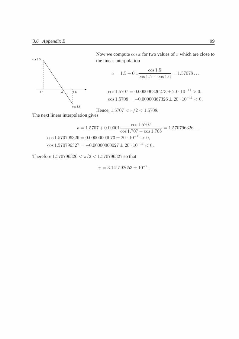
3.6 Appendix B 99
1.5 1.6
cos 1.5
cos 1.6
a
Now we computecos x for two values ofx which are close tothe linear interpolation
a = 1.5 + 0.1cos 1.5
cos 1.5− cos 1.6= 1.57078 . . .
cos 1.5707 = 0.000096326273± 20 · 10−11 > 0,
cos 1.5708 = −0.00000367326± 20 · 10−11 < 0.
Hence,1.5707 < π/2 < 1.5708.The next linear interpolation gives
b = 1.5707 + 0.00001cos 1.5707
cos 1.707− cos 1.708= 1.570796326 . . .
cos 1.570796326 = 0.00000000073± 20 · 10−11 > 0,
cos 1.570796327 = −0.00000000027± 20 · 10−11 < 0.
Therefore1.570796326 < π/2 < 1.570796327 so that
π = 3.141592653± 10−9.

100 3 Functions and Continuity

Chapter 4
Differentiation
4.1 The Derivative of a Function
We define the derivative of a function and prove the main properties like product, quotient andchain rule. We relate the derivative of a function with the derivative of its inverse function. Weprove the mean value theorem and consider local extrema. Taylor’s theorem will be formulated.
Definition 4.1 Let f : (a, b)→ R be a function andx0 ∈ (a, b). If the limit
limx→x0
f(x)− f(x0)
x− x0
(4.1)
exists, we callf differentiableatx0. The limit is denoted byf ′(x0). We sayf is differentiableif f is differentiable at every pointx ∈ (a, b). We thus have associated to every functionf afunctionf ′ whose domain is the set of pointsx0 where the limit (4.1) exists;f ′ is called thederivativeof f .
Sometimes the Leibniz notation is used to denote the derivative of f
f ′(x0) =df(x0)
dx=
d
dxf(x0).
Remarks 4.1 (a) Replacingx− x0 by h , we see thatf ′(x0) = limh→0
f(x0 + h)− f(x0)
h.
(b) The limits
limh→0−0
f(x0 + h)− f(x0)
h, lim
h→0+0
f(x0 + h)− f(x0)
h
are calledleft-hand and right-hand derivatives off in x0, respectively. In particular forf : [a, b]→ R, we can consider the right-hand derivative ata and the left-hand derivative atb.
Example 4.1 (a) Forf(x) = c the constant function
f ′(x0) = limx→x0
f(x)− f(x0)
x− x0= lim
x→x0
c− cx− x0
= 0.
(b) Forf(x) = x,
f ′(x0) = limx→x0
x− x0
x− x0
= 1.
101

102 4 Differentiation
(c) The slope of the tangent line. Given a functionf : (a, b)→ R which is differentiable atx0.Thenf ′(x0) is the slope of the tangent line to the graph off through the point(x0, f(x0)).
x1
x1
x0
y
xx0
f(
f(
)
)
α1
The slope of the secant line through(x0, f(x0)) and(x1, f(x1)) is
m = tanα1 =f(x1)− f(x0)
x1 − x0.
One can see: Ifx1 approachesx0, the secant line through(x0, f(x0)) and (x1, f(x1)) approaches the tangent linethrough(x0, f(x0)). Hence, the slope of the tangent lineis the limit of the slopes of the secant lines ifx approachesx0:
f ′(x0) = limx→x0
f(x)− f(x0)
x− x0.
Proposition 4.1 If f is differentiable atx0 ∈ (a, b), thenf is continuous atx0.
Proof. By Proposition 3.2 we have
limx→x0
(f(x)− f(x0)) = limx→x0
f(x)− f(x0)
x− x0(x− x0) = f ′(x0) lim
x→x0
(x− x0) = f ′(x0) · 0 = 0.
The converse of this proposition is not true. For examplef(x) = |x | is continuous inR but
differentiable inR \ 0 since limh→0+0
|h |h
= 1 whereas limh→0−0
|h |h
= −1. Later we will become
aquainted with a function which is continuous on the whole line without being differentiable atany point!
Proposition 4.2 Letf : (r, s)→ R be a function anda ∈ (r, s). Thenf is differentiable ata ifand only if there exists a numberc ∈ R and a functionϕ defined in a neighborhood ofa suchthat
f(x) = f(a) + (x− a)c+ ϕ(x), (4.2)
where
limx→a
ϕ(x)
x− a = 0. (4.3)
In this casef ′(a) = c.
The proposition says that a functionf differentiable ata can be approximated by a linear func-tion, in our case by
y = f(a) + (x− a)f ′(a).
The graph of this linear function is the tangent line to the graph off at the point(a, f(a)). Laterwe will use this point of view to define differentiability of functionsf : Rn → Rm.

4.1 The Derivative of a Function 103
Proof. Suppose firstf satisfies (4.2) and (4.3). Then
limx→a
f(x)− f(a)
x− a = limx→a
(c+
ϕ(x)
x− a
)= c.
Hence,f is differentiable ata with f ′(a) = c.Now, letf be differentiable ata with f ′(a) = c. Putϕ(x) = f(x)− f(a)− (x− a)f ′(a). Then
limx→a
ϕ(x)
x− a = limx→a
f(x)− f(a)
x− a − f ′(a) = 0.
f( ) α
x
x0
0
0
y
xx0
y
Q
P
(x,y)P
Let us compute the linear function whose graphis the tangent line through(x0, f(x0)). Con-sider the rectangular trianglePP0Q0. By Ex-ample 4.1 (c) we have
f ′(x0) = tanα =y − y0
x− x0
,
such that the tangent line has the equation
y = g(x) = f(x0) + f ′(x0)(x− x0).
This function is called thelinearization off at x0. It is also the Taylor polynomial of degree1of f atx0, see Section4.5 below.
Proposition 4.3 Supposef and g are defined on(a, b) and are differentible at a pointx ∈(a, b). Thenf + g, fg, andf/g are differentiable atx and
(a) (f + g)′(x) = f ′(x) + g′(x);(b) (fg)′(x) = f ′(x)g(x) + f(x)g′(x);
(c)(fg
)′(x) = f ′(x)g(x)−f(x)g′(x)
g(x)2.
In (c), we assume thatg(x) 6= 0.
Proof. (a) Since
(f + g)(x+ h)− (f + g)(x)
h=f(x+ h)− f(x)
h+g(x+ h)− g(x)
h,
the claim follows from Proposition 3.2.Let h = fg andt be variable. Then
h(t)− h(x) = f(t)(g(t)− g(x)) + g(x)(f(t)− f(x))
h(t)− h(x)t− x = f(t)
g(t)− g(x)t− x + g(x)
f(t)− f(x)
t− x .

104 4 Differentiation
Noting thatf(t)→ f(x) ast→ x, (b) follows.Next leth = f/g. Then
h(t)− h(x)t− x =
f(t)g(t)− f(x)
g(x)
t− x =f(t)g(x)− f(x)g(t)
g(x)g(t)(t− x)
=1
g(t)g(x)
f(t)g(x)− f(x)g(x) + f(x)g(x)− f(x)g(t)
t− x
=1
g(t)g(x)
(g(x)
f(t)− f(x)
t− x − f(x)g(t)− g(x)t− x
).
Letting t→ x, and applying Propositions 3.2 and 4.1, we obtain (c).
Example 4.2 (a) f(x) = xn, n ∈ Z. We will provef ′(x) = nxn−1 by induction onn ∈ N.The casesn = 0, 1 are OK by Example 4.1. Suppose the statement is true for some fixedn. Wewill show that(xn+1)′ = (n+ 1)xn.By the product rule and the induction hypothesis
(xn+1)′ = (xn · x)′ = (xn)′x+ xn(x′) = nxn−1 x+ xn = (n+ 1)xn.
This proves the claim for positive integersn. For negativen considerf(x) = 1/x−n and usethe quotient rule.(b) (ex)′ = ex.
(ex)′ = limh→0
ex+h − ex
h= lim
h→0
exeh − ex
h= ex lim
h→0
eh − 1
h= ex; (4.4)
the last equation simply follows from Example 3.9 (b)(c) (sin x)′ = cos x, (cos x)′ = − sin x. Usingsin(x+ y)− sin(x− y) = 2 cos (x) sin (y) wehave
(sin x)′ = limh→0
sin(x+ h)− sin x
h= lim
h→0
2 cos 2x+h2
sin h2
h
= limh→0
cos
(x+
h
2
)limh→0
sin h2
h2
.
Sincecosx is continuous andlimh→0
sinh
h= 1 (by the argument after Lemma 3.15), we obtain
(sin x)′ = cosx. The proof forcosx is analogous.
(d) (tanx)′ =1
cos2 x. Using the quotiont rule for the functiontan x = sin x/ cosx we have
(tanx)′ =(sin x)′ cosx− sin x(cos x)′
cos2 x=
cos2 x+ sin2 x
cos2 x=
1
cos2 x.
The next proposition deals with composite functions and is probably the most important state-ment about derivatives.
4.1 The Derivative of a Function 105
Proposition 4.4 (Chain rule) Let g : (α, β) → R be differentiable atx0 ∈ (α, β) and letf : (a, b) → R be differentiable aty0 = g(x0) ∈ (a, b). Thenh = f g is differentiable atx0, and
h′(x0) = f ′(y0)g′(x0). (4.5)
Proof. We have
f(g(x))− f(g(x0))
x− x0=f(g(x))− f(g(x0))
g(x)− g(x0)
g(x)− g(x0)
x− x0
−→x→x0
limy→y0
f(y)− f(y0)
y − y0· g′(x0) = f ′(y0)g
′(x0).
Here we used thaty = g(x) tends toy0 = g(x0) asx→ x0, sinceg is continuous atx0.
Proposition 4.5 Let f : (a, b) → R be strictly monotonic and continuous. Supposef is differ-entiable atx. Then the inverse functiong = f−1 : f((a, b)) → R is differentiable aty = f(x)
with
g′(y) =1
f ′(x)=
1
f ′(g(y)). (4.6)
Proof. Let (yn) ⊂ f((a, b)) be a sequence withyn → y andyn 6= y for all n. Putxn = g(yn).Sinceg is continuous (by Corollary 3.9),limn→∞ xn = x. Sinceg is injective,xn 6= x for all n.We have
limn→∞
g(yn)− g(y)yn − y
= limn→∞
xn − xf(xn)− f(x)
= limn→∞
1f(xn)−f(x)
xn−x=
1
f ′(x).
Henceg′(y) = 1/f ′(x) = 1/f ′(g(y)).
We give some applications of the last two propositions.
Example 4.3 (a) Letf : R → R be differentiable; defineF : R → R by F (x) := f(ax + b)
with somea, b ∈ R. ThenF ′(x) = af ′(ax+ b).
(b) In what followsf is the original function (with known derivative) andg is the inversefunction tof . We fix the notiony = f(x) andx = g(y).log : R+ \ 0 → R is the inverse function tof(x) = ex. By the above proposition
(log y)′ =1
(ex)′=
1
ex=
1
y.
(c) xα = eα log x. Hence,(xα)′ = (eα log x)′ = eα log xα1
x= αxα−1.
(d) Supposef > 0 andg = log f . Theng′ = f ′ 1
f; hencef ′ = f g′.

106 4 Differentiation
(e)arcsin : [−1, 1]→ R is the inverse function toy = f(x) = sin x. If x ∈ (−1, 1) then
(arcsin(y))′ =1
(sin x)′=
1
cos x.
Sincey ∈ [−1, 1] implies x = arcsin y ∈ [−π/2, π/2], cosx ≥ 0. Therefore,cos x =√1− sin2 x =
√1− y2. Hence
(arcsin y)′ =1√
1− y2, −1 < y < 1.
Note that the derivative is not defined at the endpointsy = −1 andy = 1.(f)
(arctan y)′ =1
(tan x)′=
11
cos2 x
= cos2 x.
Sincey = tanx we have
y2 = tan2 x =sin2 x
cos2 x=
1− cos2 x
cos2 x=
1
cos2 x− 1
cos2 x =1
1 + y2
(arctan y)′ =1
1 + y2.

4.2 The Derivatives of Elementary Functions 107
4.2 The Derivatives of Elementary Functions
function derivative
const. 0
xn (n ∈ N) nxn−1
xα (α ∈ R, x > 0) αxα−1
ex ex
ax, (a > 0) ax log a
log x1
x
loga x1
x log a
sin x cosx
cosx − sin x
tanx1
cos2 x
cotx − 1
sin2 x
sinh x cosh x
cosh x sinh x
tanhx1
cosh2 x
cothx − 1
sinh2 x
arcsin x1√
1− x2
arccosx − 1√1− x2
arctanx1
1 + x2
arccotx − 1
1 + x2
arsinh x1√
x2 + 1
arcosh x1√
x2 − 1
artanhx1
1− x2
arcothx1
1− x2

108 4 Differentiation
4.2.1 Derivatives of Higher Order
Let f : D → R be differentiable. If the derivativef ′ : D → R is differentiable atx ∈ D, then
d2f(x)
dx2= f ′′(x) = (f ′)′(x)
is called thesecond derivativeof f atx. Similarly, one defines inductively higher order deriva-tives. Continuing in this manner, we obtain functions
f, f ′, f ′′, f (3), . . . , f (k)
each of which is the derivative of the preceding one.f (n) is called thenth derivativeof f or thederivative of ordern of f . We also use the Leibniz notation
f (k)(x) =dkf(x)
dxk=
(d
dx
)kf(x).
Definition 4.2 Let D ⊂ R andk ∈ N a positive integer. We denote byCk(D) the set of allfunctionsf : D → R such thatf (k)(x) exists for allx ∈ D andf (k)(x) is continuous. ObviouslyC(D) ⊃ C1(D) ⊃ C2(D) ⊃ · · · . Further, we set
C∞(D) =⋂
k∈NCk(D) = f : D → R | f (k)(x) exists ∀ k ∈ N, x ∈ D. (4.7)
f ∈ Ck(D) is calledk times continuously differentiable. C(D) = C0(D) is the vector space ofcontinuous functions onD.
Using induction overn, one proves the following proposition.
Proposition 4.6 (Leibniz formula) Let f andg ben times differentiable. Thenfg is n timesdifferentiable with
(f(x)g(x))(n) =n∑
k=0
(n
k
)f (k)(x)g(n−k)(x). (4.8)
4.3 Local Extrema and the Mean Value Theorem
Many properties of a functionf like monotony, convexity, and existence of local extrema canbe studied using the derivativef ′. From estimates forf ′ we obtain estimates for the growth off .
Definition 4.3 Let f : [a, b]→ R be a function. We say thatf has alocal maximumat the pointξ, ξ ∈ (a, b), if there existsδ > 0 such thatf(x) ≤ f(ξ) for all x ∈ [a, b] with |x− ξ | < δ.Local minimaare defined likewise.
We say thatξ is a local extremumif it is either a local maximum or a local minimum.

4.3 Local Extrema and the Mean Value Theorem 109
Proposition 4.7 Let f be defined on[a, b]. If f has a local extremum at a pointξ ∈ (a, b), andif f ′(ξ) exists, thenf ′(ξ) = 0.
Proof. Supposef has a local maximum atξ. According with the definition chooseδ > 0 suchthat
a < ξ − δ < ξ < ξ + δ < b.
If ξ − δ < x < ξ, thenf(x)− f(ξ)
x− ξ ≥ 0.
Lettingx→ ξ, we see thatf ′(ξ) ≥ 0.If ξ < x < ξ + δ, then
f(x)− f(ξ)
x− ξ ≤ 0.
Lettingx→ ξ, we see thatf ′(ξ) ≤ 0. Hence,f ′(ξ) = 0.
Remarks 4.2 (a) f ′(x) = 0 is a necessary but not a sufficient condition for a local extremumin x. For examplef(x) = x3 hasf ′(x) = 0, butx3 has no local extremum.(b) If f attains its local extrema at the boundary, likef(x) = x on [0, 1], we do not havef ′(ξ) = 0.
Theorem 4.8 (Rolle’s Theorem)Let f : [a, b] → R be continuous withf(a) = f(b) and letfbe differentiable in(a, b). Then there exists a pointξ ∈ (a, b) with f ′(ξ) = 0.
In particular, between two zeros of a differentiable function there is a zero of its derivative.Proof. If f is the constant function, the theorem is trivial sincef ′(x) ≡ 0 on (a, b). Other-wise, there existsx0 ∈ (a, b) such thatf(x0) > f(a) or f(x0) < f(a). Thenf attains itsmaximum or minimum, respectively, at a pointξ ∈ (a, b). By Proposition 4.7,f ′(ξ) = 0.
Theorem 4.9 (Mean Value Theorem)Let f : [a, b] → R be continuous and differentiable in(a, b). Then there exists a pointξ ∈ (a, b) such that
f ′(ξ) =f(b)− f(a)
b− a (4.9)
a bξ
Geometrically, the mean value theorem states that there existsa tangent line through some point(ξ, f(ξ)) which is parallelto the secant lineAB, A = (a, f(a)),B = (b, f(b)).

110 4 Differentiation
Theorem 4.10 (Generalized Mean Value Theorem)Let f andg be continuous functions on[a, b] which are differentiable on(a, b). Then there exists a pointξ ∈ (a, b) such that
(f(b)− f(a))g′(ξ) = (g(b)− g(a))f ′(ξ).
Proof. Put
h(t) = (f(b)− f(a))g(t)− (g(b)− g(a))f(t).
Thenh is continuous in[a, b] and differentiable in(a, b) and
h(a) = f(b)g(a)− f(a)g(b) = h(b).
Rolle’s theorem shows that there existsξ ∈ (a, b) such that
h′(ξ) = f(b)− f(a))h′(ξ)− (g(b)− g(a))f ′(ξ) = 0.
The theorem follows.In case thatg′ is nonzero on(a, b) andg(b)−g(a) 6= 0, the generalized MVT states the existenceof someξ ∈ (a, b) such that
f(b)− f(a)
g(b)− g(a) =f ′(ξ)
g′(ξ).
This is in particular true forg(x) = x andg′ = 1 which gives the assertion of the Mean ValueTheorem.
Remark 4.3 Note that the MVT fails iff is complex-valued, continuous on[a, b], and differen-tiable on(a, b). Indeed,f(x) = eix on [0, 2π] is a counter example.f is continuous on[0, 2π],differentiable on(0, 2π) andf(0) = f(2π) = 1. However, there is noξ ∈ (0, 2π) such that0 = f(2π)−f(0)
2π= f ′(ξ) = ieiξ since the exponential function has no zero, see (3.7) (ez · e−z = 1)
in Subsection 3.5.1.
Corollary 4.11 Supposef is differentiable on(a, b).
If f ′(x) ≥ 0 for all x ∈ (a, b), thenf in monotonically increasing.If f ′(x) = 0 for all x ∈ (a, b), thenf is constant.If f ′(x) ≤ 0 for all x in (a, b), thenf is monotonically decreasing.
Proof. All conclusions can be read off from the equality
f(x)− f(t) = (x− t)f ′(ξ)
which is valid for each pairx, t, a < t < x < b and for someξ ∈ (t, x).

4.3 Local Extrema and the Mean Value Theorem 111
4.3.1 Local Extrema and Convexity
Proposition 4.12 Let f : (a, b) → R be differentiable and supposef ′′(ξ) exists at a pointξ ∈ (a, b). If
f ′(ξ) = 0 and f ′′(ξ) > 0,
thenf has a local minimum atξ. Similarly, if
f ′(ξ) = 0 and f ′′(ξ) < 0,
f has a local maximum atξ.
Remark 4.4 The condition of Proposition 4.12 is sufficient but not necessary for the existenceof a local extremum. For example,f(x) = x4 has a local minimum atx = 0, butf ′′(0) = 0.
Proof. We consider the casef ′′(ξ) > 0; the proof of the other case is analogous. Since
f ′′(ξ) = limx→ξ
f ′(x)− f ′(ξ)
x− ξ > 0.
By Homework 10.4 there existsδ > 0 such that
f ′(x)− f ′(ξ)
x− ξ >| f ′′(ξ) |
2> 0, for all x with 0 < | x− ξ | < δ.
Sincef ′(ξ) = 0 it follows that
f ′(x) < 0 if ξ − δ < x < ξ,
f ′(x) > 0 if ξ < x < ξ + δ.
Hence, by Corollary 4.11,f is decreasing in(ξ − δ, ξ) and increasing in(ξ, ξ + δ). Therefore,f has a local minimum atξ.
λ )yx y
f( )
x+(1-λ
f(x)+(1-λ λ )f(y)
x+(1- λ )yλ
Definition 4.4 A function f : (a, b) → R issaid to beconvexif for all x, y ∈ (a, b) and allλ ∈ [0, 1]
f(λx+ (1− λ)y) ≤ λf(x) + (1− λ)f(y).
(4.10)
A functionf is said to beconcaveif −f is con-vex.
Proposition 4.13 (a) Convex functions are continuous.(b) Supposef : (a, b)→ R is twice differentiable. Thenf is convex if and only iff ′′(x) ≥ 0 forall x ∈ (a, b).
Proof. The proof is in Appendix C to this chapter.
112 4 Differentiation
4.4 L’Hospital’s Rule
Theorem 4.14 (L’Hospital’s Rule) Supposef andg are differentiable in(a, b) andg(x) 6= 0
for all x ∈ (a, b), where−∞ ≤ a < b ≤ +∞. Suppose
limx→a+0
f ′(x)
g′(x)= A. (4.11)
If
(a) limx→a+0
f(x) = limx→a+0
g(x) = 0 or (4.12)
(b) limx→a+0
f(x) = limx→a+0
g(x) = +∞, (4.13)
then
limx→a+0
f(x)
g(x)= A. (4.14)
The analogous statements are of course also true ifx→ b− 0, or if g(x)→ −∞.
Proof. First we consider the case of finitea ∈ R. (a) One can extend the definition off andg via f(a) = g(a) = 0. Thenf andg are continuous ata. By the generalized mean valuetheorem, for everyx ∈ (a, b) there exists aξ ∈ (a, x) such that
f(x)− f(a)
g(x)− g(a) =f(x)
g(x)=f ′(ξ)
g′(ξ).
If x approachesa thenξ also approachesa, and (a) follows.(b) Now letf(a+ 0) = g(a+ 0) = +∞. Givenε > 0 chooseδ > 0 such that
∣∣∣∣f ′(t)
g′(t)− A
∣∣∣∣ < ε
if t ∈ (a, a+ δ). By the generalized mean value theorem for anyx, y ∈ (a, a+ δ) with x 6= y,∣∣∣∣f(x)− f(y)
g(x)− g(y) − A∣∣∣∣ < ε.
We havef(x)
g(x)=f(x)− f(y)
g(x)− g(y)1− g(y)
g(x)
1− f(y)f(x)
.
The right factor tends to1 asx approachesa, in particular there existsδ1 > 0 with δ1 < δ suchthatx ∈ (a, a + δ1) implies ∣∣∣∣
f(x)
g(x)− f(x)− f(y)
g(x)− g(y)
∣∣∣∣ < ε.
Further, the triangle inequality gives∣∣∣∣f(x)
g(x)− A
∣∣∣∣ < 2ε.

4.5 Taylor’s Theorem 113
This proves (b).The casex → +∞ can be reduced to the limit processy → 0 + 0 using the substitutiony = 1/x.
L’Hospital’s rule applies also applies in the casesA = +∞ andA = −∞.
Example 4.4 (a) limx→0
sin x
x= lim
x→0
cosx
1= 1.
(b) limx→0+0
√x
1− cosx= lim
x→0+0
12√x
sin x= lim
x→0+0
1
2√x sin x
= +∞.
(c)
limx→0+0
x log x = limx→0+0
log x1x
= limx→0+0
1x
− 1x2
= limx→0+0
−x = 0.
Remark 4.5 It is easy to transform other indefinite expressions to0
0or∞∞ of l’Hospital’s rule.
0 · ∞ : f · g =f1g
∞−∞ : f − g =
1g− 1
f
1fg
;
00 : f g = eg log f .
Similarly, expressions of the form1∞ and∞0 can be transformed.
4.5 Taylor’s Theorem
The aim of this section is to show hown times differentiable functions can be approximated bypolynomials of degreen.First consider a polynomialp(x) = anx
n + · · ·+ a1x+ a0. We compute
p′(x) = nanxn−1 + (n− 1)an−1x
n−2 + · · ·+ a1,
p′′(x) = n(n− 1)anxn−2 + (n− 1)(n− 2)an−1x
n−2 + · · ·+ 2a2,
...
p(n)(x) = n! an.
Insertingx = 0 givesp(0) = a0, p′(0) = a1, p′′(0) = 2a2,. . . ,p(n)(0) = n!an. Hence,
p(x) = p(0) +p′′(0)
1!x+
p′′(0)
2!x2 + · · ·+ p(n)(0)
n!xn. (4.15)
Now, fix a ∈ R and letq(x) = p(x+ a). Sinceq(k)(0) = p(k)(a), (4.15) gives
p(x+ a) = q(x) =n∑
k=0
q(k)(0)
k!xk,
p(x+ a) =n∑
k=0
p(k)(a)
k!xk.

114 4 Differentiation
Replacing in the above equationx+ a by x yields
p(x) =
n∑
k=0
p(k)(a)
k!(x− a)k. (4.16)
Theorem 4.15 (Taylor’s Theorem) Supposef is a real function on[r, s], n ∈ N, f (n) is con-tinuous on[r, s], f (n+1)(t) exists for allt ∈ (r, s). Let a andx be distinct points of[r, s] anddefine
Pn(x) =
n∑
k=0
f (k)(a)
k!(x− a)k. (4.17)
Then there exists a pointξ betweenx anda such that
f(x) = Pn(x) +f (n+1)(ξ)
(n + 1)!(x− a)n+1. (4.18)
Forn = 0, this is just the mean value theorem.Pn(x) is called thenth Taylor polynomial offat x = a, and the second summand of (4.18)
Rn+1(x, a) =f (n+1)(ξ)
(n+ 1)!(x− a)n+1
is called theLagrangian remainder term.In general, the theorem shows thatf can be approximated by a polynomial of degreen, and that(4.18) allows to estimate the error, if we know the bounds of
∣∣ f (n+1)(x)∣∣.
Proof. Considera andx to be fixed; letM be the number defined by
f(x) = Pn(x) +M(x− a)n+1
and put
g(t) = f(t)− Pn(t)−M(t− a)n+1, for r ≤ t ≤ s. (4.19)
We have to show that(n+1)!M = f (n+1)(ξ) for someξ betweena andx. By (4.17) and (4.19),
g(n+1)(t) = f (n+1)(t)− (n+ 1)!M, for r < t < s. (4.20)
Hence the proof will be complete if we can show thatg(n+1)(ξ) = 0 for someξ betweena andx.SinceP (k)
n (a) = f (k)(a) for k = 0, 1, . . . , n, we have
g(a) = g′(a) = · · · = g(n)(a) = 0.
Our choice ofM shows thatg(x) = 0, so thatg′(ξ1) = 0 for someξ1 betweena andx, byRolle’s theorem. Sinceg′(a) = 0 we conclude similarly thatg′′(ξ2) = 0 for someξ2 betweena andξ1. After n + 1 steps we arrive at the conclusion thatg(n+1)(ξn+1) = 0 for someξn+1
betweena andξn, that is, betweena andx.
4.5 Taylor’s Theorem 115
Definition 4.5 Suppose thatf is a real function defined on[r, s] such thatf (n)(t) exists for allt ∈ (r, s) and alln ∈ N. Let x anda points of[r, s]. Then
Tf (x) =∞∑
k=0
f (k)(a)
k!(x− a)k (4.21)
is called theTaylor seriesof f ata.
Remarks 4.6 (a) The radiusr of convergence of a Taylor series can be0.(b) If Tf converges, it may happen thatTf (x) 6= f(x). If Tf(x) at a pointa converges tof(x)
in a certain neighborhoodUr(a), r > 0, f is called to beanalyticata.
Example 4.5 We give an example for (b). Definef : R→ R via
f(x) =
e−1/x2
, if x 6= 0,
0, if x = 0.
We will show thatf ∈ C∞(R) with f (k)(0) = 0. For we will prove by induction onn that thereexists a polynomialpn such that
f (n)(x) = pn
(1
x
)e−1/x2
, x 6= 0
andf (n)(0) = 0. Forn = 0 the statement is clear takingp0(x) ≡ 1. Suppose the statement istrue forn. First, letx 6= 0 then
f (n+1)(x) =
(pn
(1
x
)e−1/x2
)′=
(− 1
x2p′n
(1
x
)+
2
x3pn
(1
x
))e−1/x2
.
Choosepn+1(t) = −p′n(t)t2 + 2pn(t)t3.
Secondly,
f (n+1)(0) = limh→0
f (n)(h)− f (n)(0)
h= lim
h→0
pn(
1h
)e−1/h2
h= lim
x→±∞xpn(x)e
−x2
= 0,
where we used Proposition 2.7 in the last equality.HenceTf ≡ 0 at0—the Taylor series is identically0—andTf(x) does not converge tof(x) ina neigborhood of0.
4.5.1 Examples of Taylor Series
(a) Power series coincide with their Taylor series.
ex =
∞∑
n=0
xn
n!, x ∈ R, ∞∑
n=0
xn =1
1− x, x ∈ (−1, 1).
(b) f(x) = log(1 + x), see Homework 13.4.

116 4 Differentiation
(c) f(x) = (1 + x)α, α ∈ R, a = 0. We have
f (k)(x) = α(α−1) · · · (α−k+1)(1+x)α−k, in particular f (k)(0) = α(α−1) · · · (α−k+1).
Therefore,
(1 + x)α =
n∑
k=1
α(α− 1) · · · (α− k + 1)
k!xk +Rn(x) (4.22)
The quotient test shows that the corresponding power seriesconverges for| x | < 1. Considerthe Lagrangian remainder term with0 < ξ < x < 1 andn + 1 > α. Then
|Rn+1(x) | =∣∣∣∣(
α
n + 1
)(1 + ξ)α−n−1xn+1
∣∣∣∣ ≤∣∣∣∣(
α
n+ 1
)xn+1
∣∣∣∣ ≤∣∣∣∣(
α
n+ 1
) ∣∣∣∣ −→ 0
asn→∞. Hence,
(1 + x)α =
∞∑
n=0
(α
n
)xn, 0 < x < 1. (4.23)
(4.23) is called thebinomial series. Its radius of convergence isR = 1. Looking at other formsof the remainder term gives that (4.23) holds for−1 < x < 1.(d) y = f(x) = arctanx. Sincey′ = 1/(1 + x2) andy′′ = −2x/(1 + x2)2 we see that
y′(1 + x2) = 1.
Differentiating thisn times and using Leibniz’s formula, Proposition 4.6 we have
n∑
k=0
(y′)(k)(1 + x2)(n−k)(n
k
)= 0.
=⇒(n
n
)y(n+1) (1 + x2) +
(n
n− 1
)y(n) 2x+
(n
n− 2
)y(n−1) 2 = 0;
x = 0 : y(n+1) + n(n− 1)y(n−1) = 0.
This yields
y(n)(0) =
0, if n = 2k,
(−1)k(2k)!, if n = 2k + 1.
Therefore,
arctanx =
n∑
k=0
(−1)k
2k + 1x2k+1 +R2n+2(x). (4.24)
One can prove that−1 < x ≤ 1 impliesR2n+2(x)→ 0 asn→∞. In particular,x = 1 gives
π
4= 1− 1
3+
1
5−+ · · · .

4.6 Appendix C 117
4.6 Appendix C
Corollary 4.16 (to the mean value theorem)Let f : R→ R be a differentiable function with
f ′(x) = cf(x) for all x ∈ R, (4.25)
wherec ∈ R is a fixed number. LetA = f(0). Then
f(x) = Aecx for all x ∈ R. (4.26)
Proof. ConsiderF (x) = f(x)e−cx. Using the product rule for derivatives and (4.25) we obtain
F ′(x) = f ′(x)e−cx + f(x)(−c)e−cx = (f ′(x)− cf ′(x)) e−cx = 0.
By Corollary 4.11,F (x) is constant. SinceF (0) = f(0) = A, F (x) = A for all x ∈ R; thestatement follows.
The Continuity of derivatives
We have seen that there exist derivativesf ′ which are not continuous at some point. However,not every function is a derivative. In particular, derivatives which exist at every point of an inter-val have one important property: The intermediate value theorem holds. The precise statementfollows.
Proposition 4.17 Supposef is differentiable on[a, b] and supposef ′(a) < λ < f ′(b). Thenthere is a pointx ∈ (a, b) such thatf ′(x) = λ.
Proof. Putg(t) = f(t) − λt. Theng is differentiable andg′(a) < 0. Therefore,g(t1) < g(a)
for somet1 ∈ (a, b). Similarly, g′(b) > 0, so thatg(t2) < g(b) for somet2 ∈ (a, b). Hence,g attains its minimum in theopeninterval(a, b) in some pointx ∈ (a, b). By Proposition 4.7,g′(x) = 0. Hence,f ′(x) = λ.
Corollary 4.18 If f is differentiable on[a, b], thenf ′ cannot have discontinuities of the firstkind.
Proof of Proposition 4.13. (a) Suppose first thatf ′′ ≥ 0 for all x. By Corollary 4.11,f ′ isincreasing. Leta < x < y < b andλ ∈ [0, 1]. Putt = λx+ (1− λ)y. Thenx < t < y and bythe mean value theorem there existξ1 ∈ (x, t) andξ2 ∈ (t, y) such that
f(t)− f(x)
t− x = f ′(ξ1) ≤ f ′(ξ2) =f(y)− f(t)
y − t .
Sincet− x = (1− λ)(y − x) andy − t = λ(y − x) it follows that
f(t)− f(x)
1− λ ≤ f(y)− f(t)
λ
=⇒ f(t) ≤ λf(x) + (1− λ)f(y).

118 4 Differentiation
Hence,f is convex.(b) Let f : (a, b) → R be convex and twice differentiable. Suppose to the contraryf ′′(x0) < 0
for somex0 ∈ (a, b). Let c = f ′(x0); put
ϕ(x) = f(x)− (x− x0)c.
Thenϕ : (a, b) → R is twice differentiable withϕ′(x0) = 0 andϕ′′(x0) < 0. Hence, byProposition 4.12,ϕ has a local maximum inx0. By definition, there is aδ > 0 such thatUδ(x0) ⊂ (a, b) and
ϕ(x0 − δ) < ϕ(x0), ϕ(x0 + δ) < ϕ(x0).
It follows that
f(x0) = ϕ(x0) >1
2(ϕ(x0 − δ) + ϕ(x0 + δ)) =
1
2(f(x0 − δ) + f(x0 + δ)) .
This contradicts the convexity off if we setx = x0 − δ, y = x0 + δ, andλ = 1/2.

Chapter 5
Integration
In the first section of this chapter derivatives will not appear! Roughly speaking, integrationgeneralizes “addition”. The formuladistance = velocity × time is only valid for constantvelocity. The right formula iss =
∫ t1t0v(t) dt. We need integrals to compute length of curves,
areas of surfaces, and volumes.The study of integrals requires a long preparation, but oncethis preliminary work has beencompleted, integrals will be an invaluable tool for creating new functions, and the derivativewill reappear more powerful than ever. The relation betweenthe integral and derivatives isgiven in the Fundamental Theorem of Calculus.
a b
What’s the area ??
The integral formalizes a simple intuitive concept—that ofarea. It is not a surprise that to learn the definition of an intu-itive concept can present great difficulties—“area” is certainlynot an exception.
5.1 The Riemann–Stieltjes Integral
In this section we will only define the area of some very special regions—those which arebounded by the horizontal axis, the vertical lines through(a, 0) and(b, 0) and the graph of afunctionf such thatf(x) ≥ 0 for all x in [a, b]. If f is negative on a subinterval of[a, b], theintegral will represent the difference of the areas above and below thex-axis.All intervals [a, b] are finite intervals.
Definition 5.1 Let [a, b] be an interval. By apartition of [a, b] we mean a finite set of pointsx0, x1, . . . , xn, where
a = x0 ≤ x1 ≤ · · · ≤ xn = b.
We write
∆xi = xi − xi−1, i = 1, . . . , n.
119

120 5 Integration
Now supposef is a bounded real function defined on[a, b]. Corresponding to each partitionPof [a, b] we put
x1
x=0
a x2
x=3 b
Mi = supf(x) | x ∈ [xi−1, xi] (5.1)
mi = inff(x) | x ∈ [xi−1, xi] (5.2)
U(P, f) =n∑
i=1
Mi∆xi, L(P, f) =n∑
i=1
mi∆xi, (5.3)
and finally
∫ b
a
f dx = inf U(P, f), (5.4)
∫ b
a
f dx = supL(P, f), (5.5)
where the infimum and supremum are taken over all partitionsP of [a, b]. The left members of(5.4) and (5.5) are called theupperandlower Riemann integralsof f over[a, b], respectively.If the upper and lower integrals are equal, we say thatf Riemann-integrable on[a, b] and wewrite f ∈ R (that isR denotes the Riemann-integrable functions), and we denote the commonvalue of (5.4) and (5.5) by
∫ b
a
f dx or by∫ b
a
f(x) dx. (5.6)
This is theRiemann integralof f over[a, b].
Sincef is bounded, there exist two numbersm andM such thatm ≤ f(x) ≤ M for allx ∈ [a, b]. Hence for every partitionP
m(b− a) ≤ L(P, f) ≤ U(P, f) ≤M(b− a),
so that the numbersL(P, f) andU(P, f) form a bounded set. This shows that the upper and thelower integrals are defined foreverybounded functionf . The question of their equality, andhence the question of the integrability off , is a more delicate one. Instead of investigating itseparately for the Riemann integral, we shall immediately consider a more general situation.
Definition 5.2 Let α be a monotonically increasing function on[a, b] (sinceα(a) andα(b) arefinite, it follows thatα is bounded on[a, b]). Corresponding to each partitionP of [a, b], wewrite
∆αi = α(xi)− α(xi−1).
It is clear that∆αi ≥ 0. For any real functionf which is bounded on[a, b] we put
U(P, f, α) =
n∑
i=1
Mi∆αi, (5.7)
L(P, f, α) =n∑
i=1
mi∆αi, (5.8)

5.1 The Riemann–Stieltjes Integral 121
whereMi andmi have the same meaning as in Definition 5.1, and we define
∫ b
a
f dα = inf U(P, f, α), (5.9)
∫ b
a
f dα = supU(P, f, α), (5.10)
where the infimum and the supremum are taken over all partitionsP .If the left members of (5.9) and (5.10) are equal, we denote their common value by
∫ b
a
f dα or sometimes by∫ b
a
f(x) dα(x). (5.11)
This is theRiemann–Stieltjes integral(or simply theStieltjes integral) of f with respect toα,over [a, b]. If (5.11) exists, we say thatf is integrable with respect toα in the Riemann sense,and writef ∈ R(α).
By takingα(x) = x, the Riemann integral is seen to be a special case of the Riemann–Stieltjesintegral. Let us mention explicitely, that in the general case,α need not even be continuous.We shall now investigate the existence of the integral (5.11). Without saying so every time,fwill be assumed real and bounded, andα increasing on[a, b].
Definition 5.3 We say that a partitionP ∗ is a refinementof the partitionP if P ∗ ⊃ P (thatis, every point ofP is a point ofP ∗). Given two partitions,P1 andP2, we say thatP ∗ is theircommon refinementif P ∗ = P1 ∪ P2.
Lemma 5.1 If P ∗ is a refinement ofP , then
L(P, f, α) ≤ L(P ∗, f, α) and U(P, f, α) ≥ U(P ∗, f, α). (5.12)
Proof. We only prove the first inequality of (5.12); the proof of thesecond one is analogous.Suppose first thatP ∗ contains just one point more thanP . Let this extra point bex∗, andsupposexi−1 ≤ x∗ < xi, wherexi−1 andxi are two consecutive points ofP . Put
w1 = inff(x) | x ∈ [xi−1, x∗], w2 = inff(x) | x ∈ [x∗, xi].
Clearly,w1 ≥ mi andw2 ≥ mi (sinceinfM ≥ infN if M ⊂ N , see homework 1.4 (b)),where, as before,mi = inff(x) | x ∈ [xi−1, xi]. Hence
L(P ∗, f, α)− L(P, f, α) = w1(α(x∗)− α(xi−1)) + w2(α(xi)− α(x∗))−mi(α(xi)− α(xi−1))
= (w1 −mi)(α(x∗)− α(xi−1)) + (w2 −mi)(α(xi)− α(x∗)) ≥ 0.
If P ∗ containsk points more thanP , we repeat this reasoningk times, and arrive at (5.12).

122 5 Integration
Proposition 5.2 ∫ b
a
f dα ≤∫ b
a
f dα.
Proof. LetP ∗ be the common refinement of two partitionsP1 andP2. By Lemma 5.1
L(P1, f, α) ≤ L(P ∗, f, α) ≤ U(P ∗, f, α) ≤ U(P2, f, α).
Hence
L(P1, f, α) ≤ U(P2, f, α). (5.13)
If P2 is fixed and the supremum is taken over allP1, (5.13) gives∫ b
a
f dα ≤ U(P2, f, α). (5.14)
The proposition follows by taking the infimum over allP2 in (5.14).
Proposition 5.3 (Riemann Criterion) f ∈ R(α) on [a, b] if and only if for everyε > 0 thereexists a partitionP such that
U(P, f, α)− L(P, f, α) < ε. (RC)
Proof. For everyP we have
L(P, f, α) ≤∫ b
a
f dα ≤∫ b
a
f dα ≤ U(P, f, α).
Thus (RC) implies
0 ≤∫ b
a
f dα−∫ b
a
f dα < ε.
since the above inequality can be satisfied for everyε > 0, we have
∫ b
a
f dα =
∫ b
a
f dα,
that isf ∈ R(α).Conversely, supposef ∈ R(α), and letε > 0 be given. Then there exist partitionsP1 andP2
such that
U(P2, f, α)−∫ b
a
f dα <ε
2,
∫ b
a
f dα− L(P1, f, α) <ε
2. (5.15)
We chooseP to be the common refinement ofP1 andP2. Then Lemma 5.1, together with(5.15), shows that
U(P, f, α) ≤ U(P2, f, α) <
∫ b
a
f dα +ε
2< L(P1, f, α) + ε ≤ L(P, f, α) + ε,

5.1 The Riemann–Stieltjes Integral 123
so that (RC) holds for this partitionP .
Proposition 5.3 furnishes a convenient criterion for integrability. Before we apply it, we statesome closely related facts.
Lemma 5.4 (a) If (RC) holds forP and someε, then(RC) holds with the sameε for everyrefinement ofP .(b) If (RC)holds forP = x0, . . . , xn and ifsi, ti are arbitrary points in[xi−1, xi], then
n∑
i=1
| f(si)− f(ti) |∆αi < ε.
(c) If f ∈ R(α) and (RC)holds as in(b), then∣∣∣∣∣
n∑
i=1
f(ti)∆αi −∫ b
a
f dα
∣∣∣∣∣ < ε.
Proof. Lemma 5.1 implies (a). Under the assumptions made in (b), both f(si) andf(ti) lie in[mi,Mi], so that| f(si)− f(ti) | ≤Mi −mi. Thus
n∑
i=1
| f(ti)− f(si) |∆αi ≤ U(P, f, α)− L(P, f, α),
which proves (b). The obvious inequalities
L(P, f, α) ≤∑
i
f(ti)∆αi ≤ U(P, f, α)
and
L(P, f, α) ≤∫ b
a
f dα ≤ U(P, f, α)
prove (c).
Theorem 5.5 If f is continuous on[a, b] thenf ∈ R(α) on [a, b].
Proof. Let ε > 0 be given. Chooseη > 0 so that
(α(b)− α(a))η < ε.
Sincef is uniformly continuous on[a, b] (Proposition 3.7), there exists aδ > 0 such that
| f(x)− f(t) | < η (5.16)
if x, t ∈ [a, b] and|x− t | < δ. If P is any partition of[a, b] such that∆xi < δ for all i, then(5.16) implies that
Mi −mi ≤ η, i = 1, . . . , n (5.17)

124 5 Integration
and therefore
U(P, f, α)− L(P, f, α) =
n∑
i=1
(Mi −mi)∆αi ≤ η
n∑
i=1
∆αi = η(α(b)− α(a)) < ε.
By Proposition 5.3,f ∈ R(α).
Example 5.1 (a) The proof of Theorem 5.5 together with Lemma 5.4 shows that∣∣∣∣∣
n∑
i=1
f(ti)∆αi −∫ b
a
f dα
∣∣∣∣∣ < ε
if ∆xi < δ.We computeI =
∫ ba
sin x dx. Let ε > 0. Sincesin x is continuous,f ∈ R. There existsδ > 0
such that|x− t | < δ implies
| sin x− sin t | < ε
b− a. (5.18)
In this case (RC) is satisfied and consequently∣∣∣∣∣
n∑
i=1
sin(ti)∆xi −∫ b
a
sin x dx
∣∣∣∣∣ < ε
for every partitionP with ∆xi < δ, i = 1, . . . , n.
For we choose an equidistant partition of[a, b], xi = a + (b − a)i/n, i = 0, . . . , n. Then
h = ∆xi = (b− a)/n and the condition (5.18) is satisfied providedn >(b− a)2
ε. We have, by
addition the formulacos(x− y)− cos(x+ y) = 2 sin x sin y
n∑
i=1
sin xi ∆xi =n∑
i=1
sin(a+ ih)h =h
2 sinh/2
n∑
i=1
2 sinh/2 sin(a+ ih)
=h
2 sinh/2
n∑
i=1
(cos(a+ (i− 1/2)h)− cos(a+ (i+ 1/2)h))
=h
2 sinh/2(cos(a + h/2)− cos(a+ (n+ 1/2)h))
=h/2
sinh/2(cos(a+ h/2)− cos(b+ h/2)))
Sincelimh→0 sin h/h = 1 andcos x is continuous, we find that the above expression tends tocos a− cos b. Hence
∫ ba
sin x dx = cos a− cos b.(b) Forx ∈ [a, b] define
f(x) =
1, x ∈ Q,0, x 6∈ Q.
We will show f 6∈ R. Let P be any partition of[a, b]. Since any interval contains rationalas well as irrational points,mi = 0 andMi = 1 for all i. HenceL(P, f) = 0 whereas

5.1 The Riemann–Stieltjes Integral 125
U(P, f) =∑n
i=1 ∆xi = b − a. We conclude that the upper and lower Riemann integrals don’tcoincide;f 6∈ R. A similar reasoning showsf 6∈ R(α) if α(b) > α(a) sinceL(P, f, α) = 0 <
U(P, f, α) = α(b)− α(a).
Proposition 5.6 If f is monotonic on[a, b], andα is continuous on[a, b], thenf ∈ R(α).
Proof.
(x)α
x x2b
n-1a x
1
Let ε > 0 be given. For any positiveintegern, choose a partition such that
∆αi =α(b)− α(a)
n, i = 1, . . . , n.
This is possible by the intermediatevalue theorem (Theorem 3.5) sinceαis continuous.
We suppose thatf is monotonically increasing (the proof is analogous in the other case). Then
Mi = f(xi), mi = f(xi−1), i = 1, . . . , n,
so that
U(P, f, α)− L(P, f, α) =α(b)− α(a)
n
n∑
i=1
(f(xi)− f(xi−1))
=α(b)− α(a)
n(f(b)− f(a)) < ε
if n is taken large enough. By Proposition 5.3,f ∈ R(α).
Without proofs which can be found in [Rud76, pp. 126 –128] we note the following facts.
Proposition 5.7 If f is bounded on[a, b], f has finitely many points of discontinuity on[a, b],andα is continuous at every point at whichf is discontinuous. Thenf ∈ R(α).
Proof. We give an idea of the proof in case of the Riemann integral (α(x) = x) and one singlediscontinuity atc, a < c < b. For, letε > 0 be given andm ≤ f(x) ≤ M for all x ∈ [a, b] andputC = M −m. First choose pointa′ andb′ with a < a′ < c < b′ < b andC(b′ − a′) < ε.Let fj , j = 1, 2, denote the restriction off to the subintervalsI1 = [a, a′] andI2 = [b, b′],respectively. Sincefj is continuous onIj, fj ∈ R over Ij and therefore, by the Riemanncriterion, there exist partitionsPj , j = 1, 2, of Ij such thatU(Pj , fj)− L(Pj , fj) < ε, j = 1, 2.Let P = P1 ∪ P2 be a partition of[a, b]. Then
U(P, f)− L(P, f) = U(P1, f1)− L(P1, f) + U(P2, f)− L(P2, f) + (M0 −m0)(b′ − a′)
≤ ε+ ε+ C(b′ − a′) < 3ε,
126 5 Integration
whereM0 andm0 are the supremum and infimum off(x) on [a′, b′]. The Riemann criterion issatisfied forf on [a, b], f ∈ R.
Proposition 5.8 If f ∈ R(α) on [a, b], m ≤ f(x) ≤ M , ϕ is continuous on[m,M ], andh(x) = ϕ(f(x)) on [a, b]. Thenh ∈ R(α) on [a, b].
Remark 5.1 (a) A bounded functionf is Riemann-integrable on[a, b] if and only if f is con-tinuous almost everywhere on[a, b]. (The proof of this fact can be found in [Rud76, Theo-rem 11.33]).“Almost everywhere” means that the discontinuities form a set of (Lebesgue) measure0. A setM ⊂ R has measure0 if for givenε > 0 there exist intervalsIn, n ∈ N such thatM ⊂ ⋃n∈N Inand
∑n∈N | In | < ε. Here,| I | denotes the length of the interval. Examples of sets of measure
0 are finite sets, countable sets, and the Cantor set (which is uncountable).(b) Note that such a “chaotic” function (at point0) as
f(x) =
cos 1
x, x 6= 0,
0, x = 0,
is integrable on[−π, π] since there is only one single discontinuity at0.
5.1.1 Properties of the Integral
Proposition 5.9 (a) If f1, f2 ∈ R(α) on [a, b] then f1 + f2 ∈ R(α), cf ∈ R(α) for everyconstantc and
∫ b
a
(f1 + f2) dα =
∫ b
a
f1 dα +
∫ b
a
f2 dα,
∫ b
a
cf dα = c
∫ b
a
f dα.
(b) If f1, f2 ∈ R(α) andf1(x) ≤ f2(x) on [a, b], then
∫ b
a
f1 dα ≤∫ b
a
f2 dα.
(c) If f ∈ R(α) on [a, b] and ifa < c < b, thenf ∈ R(α) on [a, c] and on[c, b], and
∫ b
a
f dα =
∫ c
a
f dα +
∫ b
c
f dα.
(d) If f ∈ R(α) on [a, b] and| f(x) | ≤M on [a, b], then∣∣∣∣∫ b
a
f dα
∣∣∣∣ ≤ M(α(b)− α(a)).
(e) If f ∈ R(α1) andf ∈ R(α2), thenf ∈ R(α1 + α2) and
∫ b
a
fd(α1 + α2) =
∫ b
a
fdα1 +
∫ b
a
fdα2;

5.1 The Riemann–Stieltjes Integral 127
if f ∈ R(α) andc is a positive constant, thenf ∈ R(cα) and∫ b
a
fd(cα) = c
∫ b
a
f dα.
Proof. If f = f1 + f2 andP is any partition of[a, b], we have
L(P, f1, α) + L(P, f2, α) ≤ L(P, f, α) ≤ U(P, f, α) ≤ U(P, f1, α) + U(P, f2, α) (5.19)
sinceinfIif1 + inf
Iif2 ≤ inf
Ii(f1 + f2) andsup
Ii
f1 + supIi
f2 ≥ supIi
(f1 + f2).
If f1 ∈ R(α) andf2 ∈ R(α), let ε > 0 be given. There are partitonsPj, j = 1, 2, such that
U(Pj , fj , α)− L(Pj, fj , α) < ε.
These inequalities persist ifP1 andP2 are replaced by their common refinementP . Then (5.19)implies
U(P, f, α)− L(P, f, α) < 2ε
which proves thatf ∈ R(α). With the sameP we have
U(P, fj, α) <
∫ b
a
fj dα + ε, j = 1, 2;
sinceL(P, f, α) <∫ baf dα < U(P, f, α); hence (5.19) implies∫ b
a
f dα ≤ U(P, f, α) <
∫ b
a
f1 dα +
∫ b
a
f2 dα + 2ε.
Sinceε was arbitrary, we conclude that∫ b
a
f dα ≤∫ b
a
f1 dα +
∫ b
a
f2 dα. (5.20)
If we replacef1 andf2 in (5.20) by−f1 and−f2, respectively, the inequality is reversed, andthe equality is proved.(b) Putf = f2−f1. It suffices to prove that
∫ baf dα ≥ 0. For every partitionP we havemi ≥ 0
sincef ≥ 0. Hence ∫ b
a
f dα ≥ L(P, f, α) =n∑
i=1
mi∆αi ≥ 0
since in addition∆αi = α(xi)− α(xi−1) ≥ 0 (α is increasing).The proofs of the other assertions are so similar that we omitthe details. In part (c) the point isthat (by passing to refinements) we may restrict ourselves topartitions which contain the pointc, in approximating
∫ baf dα, cf. Homework 14.5.
Note that in (c),f ∈ R(α) on [a, c] and on[c, b] in general does not imply thatf ∈ R(α) on[a, b]. For example consider the interval[−1, 1] with
f(x) = α(x) =
0, −1 ≤ x < 0,
1, 0 ≤ x ≤ 1.

128 5 Integration
Then∫ 1
0f dα = 0. The integral vanishes sinceα is constant on[0, 1]. However,f 6∈ R(α) on
[−1, 1] since for any partitionP including the point0, we haveU(P, f, α) = 1 andL(P, f, α) =
0.
Proposition 5.10 If f, g ∈ R(α) on [a, b], then(a)fg ∈ R(α);
(b) | f | ∈ R(α) and
∣∣∣∣∫ b
a
f dα
∣∣∣∣ ≤∫ b
a
| f | dα.
Proof. If we takeϕ(t) = t2, Proposition 5.8 shows thatf 2 ∈ R(α) if f ∈ R(α). The identity
4fg = (f + g)2 − (f − g)2
completes the proof of (a).If we takeϕ(t) = | t |, Proposition 5.8 shows that| f | ∈ R(α). Choosec = ±1 so thatc∫f dα ≥ 0. Then
∣∣∣∣∫f dα
∣∣∣∣ = c
∫f dα =
∫cf dα ≤
∫| f | dα,
since±f ≤ | f |.
The unit step functionor Heaviside functionH(x) is defined byH(x) = 0 if x < 0 andH(x) = 1 if x ≥ 0.
Example 5.2 (a) If a < s < b, f is bounded on[a, b], f is continuous ats, andα(x) = H(x−s),then ∫ b
a
f dα = f(s).
For the proof, consider the partitionP with n = 3; a = x0 < x1 < s = x2 < x3 = b. Then∆α1 = ∆α3 = 0, ∆α2 = 1, and
U(P, f, α) = M2, L(P, f, α) = m2.
Sincef is continuous ats, we see thatM2 andm2 converge tof(s) asx→ s.
(b) Supposecn ≥ 0 for all n = 1, . . . , N and(sn), n = 1, . . . , N , is a strictly increasing finitesequence of distinct points in(a, b). Further,α(x) =
∑Nn=1 cnH(x− sn). Then
∫ b
a
f dα =N∑
n=1
cnf(sn).
This follows from (a) and Proposition 5.9 (e).

5.1 The Riemann–Stieltjes Integral 129
Proposition 5.11 Supposecn ≥ 0 for all positive integersn ∈ N,
∑∞n=1 cn converges,(sn) is a strictly increasing se-
quence of distinct points in(a, b), and
α(x) =
∞∑
n=1
cnH(x− sn). (5.21)
Letf be continuous on[a, b]. Then
∫ b
a
f dα =
∞∑
n=1
cnf(sn). (5.22)
s s s s1 2 3 4
3
1c
2c
c
Proof. The comparison test shows that the series (5.21) convergesfor everyx. Its sumα isevidently an increasing function withα(a) = 0 andα(b) =
∑cn. Let ε > 0 be given, choose
N so that ∞∑
n=N+1
cn < ε.
Put
α1(x) =N∑
n=1
cnH(x− sn), α2(x) =∞∑
n=N+1
cnH(x− sn).
By Proposition 5.9 and Example 5.2
∫ b
a
f dα1 =
N∑
n=1
cnf(sn).
Sinceα2(b)− α2(a) < ε, by Proposition 5.9 (d),∣∣∣∣∫ b
a
f dα2
∣∣∣∣ ≤Mε,
whereM = sup | f(x) |. Sinceα = α1 + α2 it follows that∣∣∣∣∣
∫ b
a
f dα−N∑
n=1
cnf(sn)
∣∣∣∣∣ ≤Mε.
If we letN →∞ we obtain (5.22).
Proposition 5.12 Assume thatα is increasing andα′ ∈ R on [a, b]. Let f be a bounded realfunction on[a, b].Thenf ∈ R(α) if and only iffα′ ∈ R. In that case
∫ b
a
f dα =
∫ b
a
f(x)α′(x) dx. (5.23)
The statement remains true ifα is continuous on[a, b] and differentiable up to finitely manypointsc1, c2, . . . , cn.

130 5 Integration
Proof. Let ε > 0 be given and apply the Riemann criterion Proposition 5.3 toα′: There is apartitionP = x0, . . . , xn of [a, b] such that
U(P, α′)− L(P, α′) < ε. (5.24)
The mean value theorem furnishes pointsti ∈ [xi−1, xi] such that
∆αi = α(xi)− α(xi−1) = α′(ti)(xi − xi−1) = α′(ti)∆xi, for i = 1, . . . , n.
If si ∈ [xi−1, xi], thenn∑
i=1
|α′(si)− α′(ti) |∆xi < ε (5.25)
by (5.24) and Lemma 5.4 (b). PutM = sup | f(x) |. Sincen∑
i=1
f(si)∆αi =
n∑
i=1
f(si)α′(ti)∆xi
it follows from (5.25) that∣∣∣∣∣
n∑
i=1
f(si)∆αi −n∑
i=1
f(si)α′(si)∆xi
∣∣∣∣∣ ≤Mε. (5.26)
In particular,n∑
i=1
f(si)∆αi ≤ U(P, fα′) +Mε,
for all choices ofsi ∈ [xi−1, xi], so that
U(P, f, α) ≤ U(P, fα′) +Mε.
The same argument leads from (5.26) to
U(P, fα′) ≤ U(P, f, α) +Mε.
Thus
|U(P, f, α)− U(P, fα) | ≤Mε. (5.27)
Now (5.25) remains true ifP is replaced by any refinement. Hence (5.26) also remains true.We conclude that ∣∣∣∣∣
∫ b
a
f dα−∫ b
a
f(x)α′(x) dx
∣∣∣∣∣ ≤Mε.
But ε is arbitrary. Hence ∫ b
a
f dα =
∫ b
a
f(x)α′(x) dx,
for anyboundedf . The equality for the lower integrals follows from (5.26) inexactly the sameway. The proposition follows.
We now summarize the two cases.

5.1 The Riemann–Stieltjes Integral 131
Proposition 5.13 Let f be continuous on[a, b]. Except for finitely many pointsc0, c1, . . . , cnwith c0 = a and cn = b there existsα′(x) which is continuous and bounded on[a, b] \ c0, . . . , cn.Thenf ∈ R(α) and
∫ b
a
f dα =
∫ b
a
f(x)α′(x) dx+n−1∑
i=1
f(ci)(α(ci + 0)− α(ci − 0))+
f(a)(α(a+ 0)− α(a)) + f(b)(α(b)− α(b− 0)).
Proof (Sketch of proof). (a) Note thatA+i = α(ci + 0) − α(ci) andA−
i = α(ci) − α(ci − 0)
exist by Theorem 3.8. Define
α1(x) =
n−1∑
i=0
A+i H(x− ci) +
k∑
i=1
−A−i H(ci − x).
(b) Thenα2 = α− α1 is continuous.(c) Sinceα1 is piecewise constant,α′
1(x) = 0 for x 6= ck. Henceα′2(x) = α′(x). for x 6= ci.
Applying Proposition 5.12 gives
∫ b
a
fdα2 =
∫ b
a
fα′2 dx =
∫ b
a
fα′ dx.
Further, ∫ b
a
f dα =
∫ b
a
fd(α1 + α2) =
∫ b
a
fα′ dx+
∫ b
a
fdα1.
By Proposition 5.11∫ b
a
fdα1 =
n∑
i=1
A+i f(ci)−
n−1∑
i=1
A−i (−f(ci)).
Example 5.3 (a) The Fundamental Theorem of Calculus, see Theorem 5.15 yields
∫ 2
0
x dx3 =
∫ 2
0
x · 3x2 dx = 3x4
4
∣∣∣∣2
0
= 12.
(b) f(x) = x2.
α(x) =
x, 0 ≤ x < 1,
7, x = 1,
x2 + 10, 1 < x < 2,
64, x = 2.

132 5 Integration
∫ 2
0
f dα =
∫ 2
0
fα′ dx+ f(1)(α(1 + 0)− α(1− 0)) + f(2)(α(2)− α(2− 0))
=
∫ 1
0
x2 · 1 dx+
∫ 2
1
x2 · 2x dx+ 1(11− 1) + 4(64− 14)
=x3
3
∣∣∣∣1
0
+x4
2
∣∣∣∣2
1
+ 10 + 200 =1
3+ 8− 1
2+ 210 = 217
5
6.
Remark 5.2 The three preceding proposition show the flexibility of the Stieltjes process ofintegration. Ifα is a pure step function, the integral reduces to an infinite series. If α hasan initegrable derivative, the integral reduces to the ordinary Riemann integral. This makes itpossible to study series and integral simultaneously, rather than separately.
5.2 Integration and Differentiation
We shall see that integration and differentiation are, in a certain sense, inverse operations.
Theorem 5.14 Let f ∈ R on [a, b]. For a ≤ x ≤ b put
F (x) =
∫ x
a
f(t) dt.
ThenF is continuous on[a, b]; furthermore, iff is continuous atx0 ∈ [a, b] thenF is differen-tiable atx0 and
F ′(x0) = f(x0).
Proof. Sincef ∈ R, f is bounded. Suppose| f(t) | ≤M on [a, b]. If a ≤ x < y ≤ b, then
|F (y)− F (x) | =∣∣∣∣∫ y
x
f(t) dt
∣∣∣∣ ≤M(y − x),
by Proposition 5.9 (c) and (d). Givenε > 0, we see that
|F (y)− F (x) | < ε,
provided that| y − x | < ε/M . This proves continuity (and, in fact, uniform continuity)of F .Now suppose thatf is continuous atx0. Givenε > 0, chooseδ > 0 such that
| f(t)− f(x0) | < ε
if | t− x0 | < δ, t ∈ [a, b]. Hence, if
x0 − δ < s ≤ x0 ≤ t < x0 + δ, and a ≤ s < t ≤ b,
we have by Proposition 5.9 (d) as before∣∣∣∣F (t)− F (s)
t− s − f(x0)
∣∣∣∣ =∣∣∣∣
1
t− s
∫ t
s
f(r) dr − 1
t− s
∫ t
s
f(x0) dr
∣∣∣∣
=1
t− s
∣∣∣∣∫ t
s
(f(u)− f(x0)) du
∣∣∣∣ < ε.

5.2 Integration and Differentiation 133
This in particular holds fors = x0, that is∣∣∣∣F (t)− F (x0)
t− x0− f(x0)
∣∣∣∣ < ε.
It follows thatF ′(x0) = f(x0).
Definition 5.4 A functionF : [a, b]→ R is called anantiderivativeor aprimitiveof a functionf : [a, b]→ R if F is differentiable andF ′ = f .
Remarks 5.3 (a) There exist functionsf not having an antiderivative, for example the Heav-iside functionH(x) has a simple discontinuity at0; but by Corollary 4.18 derivatives cannothave simple discontinuities.(b) The antiderivativeF of a functionf (if it exists) is unique up to an additive constant. Moreprecisely, ifF is a antiderivative on[a, b], thenF1(x) = F (x) + c is also a antiderivative off .If F andG are antiderivatives off on [a, b], then there is a constantc so thatF (x)−G(x) = c.The first part is obvious sinceF ′
1(x) = F ′(x)+ c′ = f(x). SupposeF andG are antiderivativesof f . PutH(x) = F (x)−G(x); thenH ′(x) = 0 andH(x) is constant by Corollary 4.11.
Notation for the antiderivative:
F (x) =
∫f(x) dx =
∫f dx.
The functionf is called theintegrand. Integration and differentiation are inverse to each other:
d
dx
∫f(x) dx = f(x),
∫f ′(x) dx = f(x).
Theorem 5.15 (Fundamental Theorem of Calculus)Letf : [a, b]→ R be continuous.(a) If
F (x) =
∫ x
a
f(t) dt.
ThenF (x) is an antiderivative off(x) on [a, b].(b) If G(x) is an antiderivative off(x) then
∫ b
a
f(t) dt = G(b)−G(a).
Proof. (a) By Theorem 5.14F (x) =∫ xaf(x) dx is differentiable at any pointx0 ∈ [a, b] with
F ′(x) = f(x).(b) By the above remark, the antiderivative is unique up to a constant, henceF (x)−G(x) = C.SinceF (a) =
∫ aaf(x) dx = 0 we obtain
G(b)−G(a) = (F (b)− C)− (F (a)− C) = F (b)− F (a) = F (b) =
∫ b
a
f(x) dx.

134 5 Integration
Note that the FTC is also true iff ∈ R andG is an antiderivative off on [a, b]. Indeed, letε > 0
be given. By the Riemann criterion, Proposition 5.3 there exists a partitionP = x0, . . . , xnof [a, b] such thatU(P, f) − L(P, f) < ε. By the mean value theorem, there exist pointsti ∈ [xi−1, xi] such that
F (xi)− F (xi−1) = f(ti)(xi − xi−1), i = 1, . . . , n.
Thus
F (b)− F (a) =n∑
i=1
f(ti)∆xi.
It follows from Lemma 5.4 (c) and the above equation that∣∣∣∣∣
n∑
i=1
f(ti)∆xi −∫ b
a
f(x) dx
∣∣∣∣∣ =
∣∣∣∣F (b)− F (a)−∫ b
a
f(x) dx
∣∣∣∣ < ε.
Sinceε > 0 was arbitrary, the proof is complete.
5.2.1 Table of Antiderivatives
By differentiating the right hand side one gets the left handside of the table.
function domain antiderivative
xα α ∈ R \ −1, x > 01
α + 1xα+1
1
xx < 0 or x > 0 log | x |
ex R ex
ax a > 0, a 6= 1, x ∈ R ax
log a
sin x R − cosx
cosx R sin x
1
sin2 xR \ kπ | k ∈ Z − cot x
1
cos2 xR \
π2
+ kπ | k ∈ Z tanx
1
1 + x2R arctan x
1√1 + x2
R arsinh x = log(x+√x2 + 1)
1√1− x2
−1 < x < 1 arcsin x
1√x2 − 1
x < −1 or x > 1 log(x+√x2 − 1)
5.2 Integration and Differentiation 135
5.2.2 Integration Rules
The aim of this subsection is to calculate antiderivatives of composed functions using antideriva-tives of (already known) simpler functions.Notation:
f(x)|ba := f(b)− f(a).
Proposition 5.16 (a)Letf andg be functions with antiderivativesF andG, respectively. Thenaf(x) + bg(x), a, b ∈ R, has the antiderivativeaF (x) + bG(x).
∫(af + bg) dx = a
∫f dx+ b
∫g dx (Linearity.)
(b) If f andg are differentiable, andf(x)g′(x) has a antiderivative thenf ′(x)g(x) has a an-tiderivative, too:
∫f ′g dx = fg −
∫fg′ dx, (Integration by parts.) (5.28)
If f andg are continuously differentiable on[a, b] then
∫ b
a
f ′g dx = f(x)g(x)|ba −∫ b
a
fg′ dx. (5.29)
(c) If ϕ : D → R is continuously differentiable withϕ(D) ⊂ I, andf : I → R has a antideriva-tiveF , then
∫f(ϕ(x))ϕ′(x) dx = F (ϕ(x)), (Change of variable.) (5.30)
If ϕ : [a, b] → R is continuously differentiable withϕ([a, b]) ⊂ I andf : I → R is continuous,then
∫ b
a
f(ϕ(t))ϕ′(t) dt =
∫ ϕ(b)
ϕ(a)
f(x) dx.
Proof. Since differentiation is linear, (a) follows.(b) Differentiating the right hand side, we obtain
d
dx(fg −
∫fg′ dx) = f ′g + fg′ − fg′ = f ′g
which proves the statement.(c) By the chain ruleF (ϕ(x)) is differentiable with
d
dxF (ϕ(x)) = F ′(ϕ(x))ϕ′(x) = f(ϕ(x))ϕ′(x),
and (c) follows.The statements about the Riemann integrals follow from the statements about antiderivatives

136 5 Integration
using the fundamental theorem of calculus. For example, we show the second part of (c). Bythe above part,F (ϕ(t)) is an antiderivative off(ϕ(t))ϕ′(t). By the FTC we have
∫ b
a
f(ϕ(t))ϕ′(t) dt = F (ϕ(t))|ba = F (ϕ(b))− F (ϕ(a)).
On the other hand, again by the FTC,
∫ ϕ(b)
ϕ(a)
f(x) dx = F (x)|ϕ(b)ϕ(a) = F (ϕ(b))− F (ϕ(a)).
This completes the proof of (c).
Corollary 5.17 SupposeF is the antiderivative off .∫f(ax+ b) dx =
1
aF (ax+ b), a 6= 0; (5.31)
∫g′(x)
g(x)dx = log | g(x) | , (g differentiable andg(x) 6= 0). (5.32)
Example 5.4 (a) The antiderivative of a polymnomial. Ifp(x) =∑n
k=0 akxk, then
∫p(x) dx =∑n
k=0ak
k+1xk+1.
(b) Putf ′(x) = ex andg(x) = x, thenf(x) = ex andg′(x) = 1 and we obtain∫xex dx = xex −
∫1 · ex dx = ex(x− 1).
(c) I = (0,∞).∫
log x dx =∫
1 · log x dx = x log x−∫x 1x
dx = x log x− x.(d)
∫arctanx dx =
∫1 · arctan x dx = x arctanx−
∫x
1
1 + x2dx
= x arctan x− 1
2
∫(1 + x2)′
1 + x2dx = x arctan x− 1
2log(1 + x2).
In the last equation we made use of (5.32).(e) Recurrent computation of integrals.
In :=
∫dx
(1 + x2)n, n ∈ N.
I1 = arctanx.
In =
∫(1 + x2)− x2
(1 + x2)n= In−1 −
∫x2 dx
(1 + x2)n.
Putu = x, v′ =x
(1 + x2)n. ThenU ′ = 1 and
v =
∫x dx
(1 + x2)n=
1
2
(1 + x2)1−n
1− n .

5.2 Integration and Differentiation 137
Hence,
In = In−1 −1
2
x(1 + x2)1−n
1− n − 1
2(1− n)
∫(1 + x2)1−n dx
In =x
(2n− 2)(1 + x2)n−1+
2n− 3
2n− 2In−1.
In particular,I2 = x2(1+x2)
+ 12arctanx andI3 = x
4(1+x2)2+ 3
4I2.
Proposition 5.18 (Mean Value Theorem of Integration)Let f, ϕ : [a, b] → R be continuousfunctions andϕ ≥ 0. Then there existsξ ∈ [a, b] such that
∫ b
a
f(x)ϕ(x) dx = f(ξ)
∫ b
a
ϕ(x) dx. (5.33)
In particular, in caseϕ = 1 we have∫ b
a
f(x) dx = f(ξ)(b− a)
for someξ ∈ [a, b].
Proof. Putm = inff(x) | x ∈ [a, b] andM = supf(x) | x ∈ [a, b]. Sinceϕ ≥ 0 we obtainmϕ(x) ≤ f(x)ϕ(x) ≤Mϕ(x). By Proposition 5.9 (a) and (b) we have
m
∫ b
a
ϕ(x) dx ≤∫ b
a
f(x)ϕ(x) dx ≤M
∫ b
a
ϕ(x) dx.
Hence there is aµ ∈ [m,M ] such that∫ b
a
f(x)ϕ(x) dx = µ
∫ b
a
ϕ(x) dx.
Sincef is continuous on[a, b] the intermediate value theorem Theorem 3.5 ensures that thereis aξ with µ = f(ξ). The claim follows.
Example 5.5 The trapezoid rule. Letf : [0, 1]→ R be twice continuously differentiable. Thenthere existsξ ∈ [0, 1] such that
∫ 1
0
f(x) dx =1
2(f(0) + f(1))− 1
12f ′′(ξ). (5.34)
Proof. Letϕ(x) = 12x(1−x) such thatϕ(x) ≥ 0 for x ∈ [0, 1], ϕ′(x) = 1
2−x, andϕ′′(x) = −1.
Using integration by parts twice as well as Theorem 5.18 we find∫ 1
0
f(x) dx = −∫ 1
0
ϕ′′(x)f(x) dx = −ϕ′(x)f(x)|10 +
∫ 1
0
ϕ′(x)f ′(x) dx
=1
2(f(0) + f(1)) + ϕ(x)f ′(x)|10 −
∫ 1
0
ϕ(x)f ′′(x) dx
=1
2(f(0) + f(1))− f ′′(ξ)
∫ 1
0
ϕ(x) dx
=1
2(f(0) + f(1))− 1
12f ′′(ξ).

138 5 Integration
Indeed,∫ 1
0
(12x− 1
2x2)
dx = 14x2 − 1
6x3∣∣10
= 14− 1
6= 1
12.
5.2.3 Integration of Rational Functions
We will give a useful method to compute antiderivatives of anarbitrary rational function.Consider a rational functionp/q wherep andq are polinomials. We will assume thatdeg p <
deg q; for otherwise we can expressp/q as a polynomial function plus a rational function whichis of this form, for eample
x2
x− 1= x+ 1 +
1
x− 1.
Polynomials
We need some preliminary facts on polynomials which are stated here without proof. Recallthat a non-zero constant polynomial has degree zero,deg c = 0 if c 6= 0. By definition, the zeropolynomial has degree−∞, deg 0 = −∞.
Theorem 5.19 (Fundamental Theorem of Algebra)Every polynomialp of positive degreewith complex coefficients has a complex root, i. e. there exists a complex numberz such thatp(z) = 0.
Lemma 5.20 (Long Division) Letp andq be polynomials, then there exist unique polynomialsr ands such that
p = qs+ r, deg r < deg q.
Lemma 5.21 Let p be a complex polynomial of degreen ≥ 1 and leading coefficientan. Thenthere existn uniquely determined numbersz1, . . . , zn (which may be equal) such that
p(z) = an(z − z1)(z − z2) · · · (z − zn).
Proof. We use induction overn and the two preceding statements. In casen = 1 the linearpolynomialp(z) = az + b can be written in the desired form
p(z) = a
(z − −b
a
)with the unique root z1 = − b
a.
Suppose the statement is true for all polynomials of degreen− 1. We will show it for degreenpolynomials. For, letzn be a complex root ofpwhich exists by Theorem 5.19;p(zn) = 0. Usinglong division ofp by the linear polynomialq(z) = z−zn we obtain a quotient polynomialp1(z)
and a remainder polynomialr(z) of degree0 (a constant polynomial) such that
p(z) = (z − zn)p1(z) + r(z).
Insertingz = zn givesp(zn) = 0 = r(zn); hence the constantr vanishes and we have
p(z) = (z − zn)p1(z)

5.2 Integration and Differentiation 139
with a polynomialp1(z) of degreen− 1. Applying the induction hypothesis top1 the statementfollows.
A root α of p is said to be aroot of multiplicityk, k ∈ N, if α appears exactlyk times amongthe zerosz1, z2, . . . , zn. In that case(z − α)k dividesp(z) but (z − α)k+1 not.If p is a real polynomial, i. e. a polynomial with real coefficients, andα is a root of multiplicityk of p thenα is also a root of multiplicityk of p. Indeed, taking the complex conjugation of theequation
p(z) = (z − α)kq(z)
we have sincep(z) = p(z) = p(z)
p(z) = (z − α)kq(z) =⇒z:=z
p(z) = (z − α)kq(z).
Note that the product of the two complex linear factorsz − α andz − α yield a real quadraticfactor
(z − α)(z − α) = z2 − (α + α)z + αα = z2 − 2 Reα + |α |2 .
Using this fact, the real version of Lemma 5.21 is as follows.
Lemma 5.22 Let q be a real polynomial of degreen with leading coefficientan. Then thereexist real numbersαi, βj , γj and multiplicitiesri, sj ∈ N, i = 1, . . . , k, j = 1, . . . , l such that
q(x) = an
k∏
i=1
(x− αi)ril∏
j=1
(x2 − 2βjx+ γj)sj .
We assume that the quadratic factors cannot be factored further; this means
β2j − γj < 0, j = 1, . . . , l.
Of course,deg q =∑
i ri +∑
j 2sj = n.
Example 5.6 (a) x4 − 4 = (x2 + 2)(x2 − 2) = (x −√
2)(x +√
2)(x − i√
2)(x + i√
2) =
(x−√
2)(x+√
2)(x2 + 2)
(b) x3 + x− 2. One can guess the first zerox1 = 1. Using long division one gets
x3 +x −2 = (x− 1)(x2 + x+ 2)
−(x3 −x2)
x2 +x −2
−(x2 −x )
2x −2
−(2x −2)
0
There are no further real zeros ofx2 + x+ 2.

140 5 Integration
5.2.4 Partial Fraction Decomposition
Proposition 5.23 Let p(x) andq(x) be real polynomials withdeg p < deg q. There exist realnumbersAir, Bjs, andCjs such that
p(x)
q(x)=
k∑
i=1
(ri∑
r=1
Air(x− αi)r
)+
l∑
j=1
(sj∑
s=1
Bjsx+ Cjs(x2 − 2βjx+ γj)s
)(5.35)
where theαi, βj , γj, ri, andsj have the same meaning as in Lemma 5.22.
Example 5.7 (a) Compute∫f(x) dx =
∫x4
x3 − 1dx. We use long division to obtain a ratio-
nal functionp/q with deg p < deg q, f(x) = x+ xx3−1
. To obtain the partial fraction decompo-sition (PFD), we need the factorization of the denominator polynomialq(x) = x3 − 1. One canguess the first real zerox1 = 1 and divideq by x− 1; q(x) = (x− 1)(x2 + x+ 1).The PFD then reads
x
x3 − 1=
a
x− 1+
bx+ c
x2 + x+ 1.
We have to determinea, b, c. Multiplication byx3 − 1 gives
0 · x2 + 1 · x+ 0 = a(x2 + x+ 1) + (bx+ c)(x− 1) = (a+ b)x2 + (a− b+ c)x+ a− c.
The two polynomials on the left and on the right must coincide, that is, there coefficients mustbe equal:
0 = a− c, 1 = a− b+ c, 0 = a+ b;
which givesa = −b = c = 13. Hence,
x
x3 − 1=
1
3
1
x− 1− 1
3
x− 1
x2 + x+ 1.
We can integrate the first two terms but we have to rewrite the last one
x− 1
x2 + x+ 1=
1
2
2x+ 1
x2 + x+ 1− 3
2
1(x+ 1
2
)2+ 3
4
.
Recall that∫
2x− 2β
x2 − 2βx+ γdx = log
∣∣ x2 − 2βx+ γ∣∣ ,
∫dx
(x+ b)2 + a2=
1
aarctan
x+ b
a.
Therefore,∫
x4
x3 − 1dx =
1
2x2 +
1
2log |x− 1 | − 1
6log(x2 + x+ 1) +
1√3
arctan2x+ 1√
3.
(b) If q(x) = (x−1)3(x+2)(x2+2)2(x2 +1) andp(x) is any polynomial withdeg p < deg q =
10, then the partial fraction decomposition reads as
p(x)
q(x)=
A11
x− 1+
A12
(x− 1)2+
A13
(x− 1)3+
A21
x+ 2+B11x+ C11
x2 + 2+B12x+ C12
(x2 + 2)2+B21 + C21
x2 + 1.
(5.36)

5.2 Integration and Differentiation 141
Suppose now thatp(x) ≡ 1. One can immediately computeA13 andA21. Multiplying (5.36)by (x− 1)3 yields
1
(x+ 2)(x2 + 2)2(x2 + 1)= A13 + (x− 1)p1(x)
with a rational functionp1 not having(x − 1) in the denominator. Insertingx = 1 givesA13 = 1
32·3·2 = 154
. Similarly,
A21 =1
(x− 1)3(x2 + 2)2(x2 + 1)
∣∣∣∣x=−2
=1
(−3)3 · 6 · 5 .
5.2.5 Other Classes of Elementary Integrable Functions
An elementary functionis the compositions of rational, exponential, trigonometric functionsand their inverse functions, for example
f(x) =esin(
√x−1)
x+ log x.
A function is calledelementary integrableif it has an elementary antiderivative. Rational func-tions are elementary integrable. “Most” functions are not elementary integrable as
e−x2
,ex
x,
1
log x,
sin x
x.
They define “new” functions
W (x) :=
∫ x
0
e−t2
2 dt, (Gaussian integral),
li(x) :=
∫ x
0
dt
log t(integral logarithm)
F(ϕ, k) :=
∫ ϕ
0
dx√1− k2 sin2 x
(elliptic integral of the first kind),
E(ϕ, k) :=
∫ ϕ
0
√1− k2 sin2 x dx (elliptic integral of the second kind).
∫R(cos x, sin x) dx
LetR(u, v) be a rational function in two variablesu andv, that isR(u, v) = p(u,v)q(u,v)
with polino-
mialsp andq in two variables. We substitutet = tanx
2. Then
sin x =2t
1 + t2, cos x =
1− t21 + t2
, dx =2dt
1 + t2.
Hence ∫R(cosx, sin x) dx =
∫R
(1− t21 + t2
,2t
1 + t2
)2dt
1 + t2=
∫R1(t) dt
with another rational functionR1(t).There are 3 special cases where another substitution is apropriate.

142 5 Integration
(a) R(−u, v) = −R(u, v), R is odd inu. Substitutet = sin x.
(b) R(u,−v) = −R(u, v), R is odd inv. Substitutet = cosx.
(c) R(−u,−v) = R(u, v). Substitutet = tan x.
Example 5.8 (1)∫
sin3 x dx. Here,R(u, v) = v3 is an odd function inv, such that (b) applies;
t = cos x, dt = − sin x dx, sin2 x = 1− cos2 x = 1− t2. This yields∫
sin3 x dx = −∫
sin2 x · (− sin x dx) = −∫
(1− t2) dt = −t+t3
3+ const.
= − cos x+cos3
3+ const. .
(2)∫
tanx dx. Here,R(u, v) = vu. All (a), (b), and (c) apply to this situation. For example, let
t = sin x. Thencos2 x = 1− t2, dt = cosx dx and
∫tanx dx =
∫sin x · cosx dx
cos2 x=
∫t dt
1− t2 = −1
2
∫d(1− t2)
1− t2 =
= −1
2log(1− t2) = − log | cosx | .
∫R(x, n
√ax + b) dx
The substitutiont =
n√ax+ b
yieldsx = (tn − b)/a, dx = ntn−1 dt/a, and therefore∫R(x,
n√ax+ b) dx =
n
a
∫R
(tn − ba
, t
)tn−1 dt.
∫R(x,
√ax2 + 2bx + c) dx
Using the method of complete squares the above integral can be written in one of the three basicforms ∫
R(t,√t2 + 1) dt,
∫R(t,√t2 − 1) dt,
∫R(t,√
1− t2) dt.
Further substitutions
t = sinh u,√t2 + 1 = cosh u, dt = cosh u du,
t = ± cosh u,√t2 − 1 = sinh u, dt = ± sinh u du,
t = ± cos u,√
1− t2 = sin u, dt = ∓ sin u du
reduce the integral to already known integrals.

5.3 Improper Integrals 143
Example 5.9 ComputeI =
∫dx√
x2 + 6x+ 5. Hint: t =
√x2 + 6x+ 5− x.
Then(x+ t)2 = x2 +2tx+ t2 = x2 +6x+5 such thatt2 +2tx = 6x+5 and thereforex = t2−56−2t
and
dx =2t(6− 2t) + 2(t2 − 5)
(6− 2t)2dt =
−2t2 + 12t− 10
(6− 2t)2dt.
Hence, usingt+ x = t+ t2−56−2t
= −t2+6t−56−2t
,
I =
∫(−2t2 + 12t− 10) dt
(6− 2t)2
1
t+ x=
∫2(6− 2t)(−t2 + 6t− 5)
(−t2 + 6t− 5)(6− 2t)2dt
= 2
∫dt
6− 2t= − log | 6− 2t |+ const. = log
∣∣∣ 6− 2√x2 + 6x+ 5 + 2x
∣∣∣ + const.
5.3 Improper Integrals
The notion of the Riemann integral defined so far is apparently too tight for some applications:we can integrate only over finite intervals and the functionsare necessarily bounded. If theintegration interval is unbounded or the function to integrate is unbounded we speak aboutimproperintegrals. We consider three cases: one limit of the integral is infinite; the function isnot defined at one of the end pointsa or b of the interval; botha andb are critical points (eitherinfinity or the function is not defined there).
5.3.1 Integrals on unbounded intervals
Definition 5.5 Supposef ∈ R on [a, b] for all b > a wherea is fixed. Define
∫ ∞
a
f(x) dx = limb→+∞
∫ b
a
f(x) dx (5.37)
if this limit exists (and is finite). In that case, we say that the integral on the leftconverges. If italso converges iff has been replaced by| f |, it is said toconverge absolutely.
If an integral converges absolutely, then it converges, seeExample 5.11 below, where
∣∣∣∣∫ ∞
a
f dx
∣∣∣∣ ≤∫ ∞
a
| f | dx.
Similarly, one defines∫ b
−∞f(x) dx. Moreover,
∫ ∞
−∞f dx :=
∫ 0
−∞f dx+
∫ ∞
0
f dx
if both integrals on the right side converge.

144 5 Integration
Example 5.10 (a) The integral∫ ∞
1
dx
xsconverges fors > 1 and diverges for0 < s ≤ 1.
Indeed,∫ R
1
dx
xs=
1
1− s ·1
xs−1
∣∣∣∣R
1
=1
s− 1
(1− 1
Rs−1
).
Since
limR→+∞
1
Rs−1=
0, if s > 1,
+∞, if 0 < s < 1,
it follows that ∫ ∞
0
dx
xs=
1
s− 1, if s > 1.
(b) ∫ R
0
e−x dx = −e−x∣∣R0
= 1− 1
eR.
Hence∫ ∞
0
e−x dx = 1.
Proposition 5.24 (Cauchy criterion) The improper integral∫ ∞
a
f dx converges if and only if
for everyε > 0 there exists someb > a such that for allc, d > b∣∣∣∣∫ d
c
f dx
∣∣∣∣ < ε.
Proof. The followingCauchy criterion for limits of functionsis easily proved using sequences:
The limit limx→∞
F (x) exists if and only if
∀ ε > 0 ∃R > 0 ∀x, y > R : |F (x)− F (y) | < ε. (5.38)
Indeed, suppose that(xn) is any sequence converging to+∞ as n → ∞. We will showthat (F (xn)) converges if (5.38) is satisfied. Letε > 0. By assumption, there existsR > 0
with the above property. Sincexn −→n→∞
+∞ there existsn0 ∈ N such thatn ≥ n0 implies
xn > R. Hence,|F (xn)− F (xm) | < ε asm,n ≥ n0. Thus,(F (xn)) is a Cauchy sequence andtherefore convergent. This proves one direction of the above criterion. The inverse direction iseven simpler: Suppose thatlim
x→+∞F (x) = A exists (and is finite!). We will show that the above
criterion is satisfied.Letε > 0. By definition of the limit there existsR > 0 such thatx, y > R
imply |F (x)−A | < ε/2 and|F (y)− A | < ε/2. By the triangle inequality,
|F (x)− F (y) | = |F (x)−A− (F (y)− A) | ≤ |F (x)− A |+ |F (y)−A | < ε
2+ε
2= ε,
asx, y > R which completes the proof of this Cauchy criterion.
Applying this criterion to the functionF (t) =∫ taf dx noting that|F (d)− F (c) | =
∣∣∣∫ dcf dx
∣∣∣,the limit limt→∞ F (t) exists.

5.3 Improper Integrals 145
Example 5.11 (a) If∫∞af dx converges absolutely, then
∫∞af dx converges. Indeed, letε > 0
and∫∞a| f | dx converges. By the Cauchy Criterion for the later integral and by the triangle
inequality, Proposition 5.10, there existsb > 0 such that for allc, d > b∣∣∣∣∫ d
c
f dx
∣∣∣∣ ≤∫ d
c
| f | dx < ε. (5.39)
Hence, the Cauchy criterion is satisfied forf if it holds for | f |. Thus,∫∞af dx converges.
(b)∫∞1
sinxx
dx. Partial integration withu = 1x
andv′ = sin x yieldsu′ = − 1x2 , v = − cos x and
∫ d
c
sin x
xdx = −1
xcosx
∣∣∣∣d
c
−∫ d
c
cosx
x2dx
∣∣∣∣∫ d
c
sin x
xdx
∣∣∣∣ ≤∣∣∣∣−
1
dcos d+
1
ccos c
∣∣∣∣+∣∣∣∣∫ d
c
dx
x2
∣∣∣∣
≤ 1
c+
1
d+
∣∣∣∣1
d− 1
c
∣∣∣∣ ≤ 2
(1
c+
1
d
)< ε
if c andd are sufficiently large. Hence,∫∞1
sinxx
dx converges.The integral does not converge absolutely. For non-negative integersn ∈ Z+ we have
∫ (n+1)π
nπ
∣∣∣∣sin x
x
∣∣∣∣ dx ≥ 1
(n+ 1)π
∫ (n+1)π
nπ
| sin x | dx =2
(n + 1)π;
hence ∫ (n+1)π
1
∣∣∣∣sin x
x
∣∣∣∣ dx ≥ 2
π
n∑
k=1
1
k + 1.
Since the harmonic series diverges, so does the integral∫∞π
∣∣ sinxx
∣∣ dx.
Proposition 5.25 Supposef ∈ R is nonnegative,f ≥ 0. Then∫∞af dx converges if there
existsC > 0 such that∫ b
a
f dx < C, for all b > a.
The proof is similar to the proof of Lemma 2.19 (c); we omit it.Analogous propositions are truefor integrals
∫ a−∞ f dx.
Proposition 5.26 (Integral criterion for series) Assume thatf ∈ R is nonnegativef ≥ 0 anddecreasing on[1,+∞). Then
∫∞1f dx converges if and only if the series
∑∞n=1 f(n) converges.
Proof. Sincef(n) ≤ f(x) ≤ f(n− 1) for n− 1 ≤ x ≤ n,
f(n) ≤∫ n
n−1
f dx ≤ f(n− 1).
Summation overn = 2, 3, . . . , N yields
N∑
n=2
f(n) ≤∫ N
1
f dx ≤N−1∑
n=1
f(n).

146 5 Integration
If∫∞1f dx converges the series
∑∞n=1 f(n) is bounded and therefore convergent.
Conversely, if∑∞
n=1 f(n) converges, the integral∫ R1f dx ≤ ∑∞
n=1 f(n) is bounded asR→∞, hence convergent by Proposition 5.25.
Example 5.12∑∞
n=21
n(logn)α converges if and only if∫∞2
dxx(log x)α converges. The substitution
y = log x, dy = dxx
gives ∫ ∞
2
dx
x(log x)α=
∫ ∞
log 2
dy
yα
which converges if and only ifα > 1 (see Example 5.10).
5.3.2 Integrals of Unbounded Functions
Definition 5.6 Supposef is a real function on[a, b) andf ∈ R on [a, t] for everyt, a < t < b.Define ∫ b
a
f dx = limt→b−0
∫ t
a
f dx
if the limit on the right exists. Similarly, one defines
∫ b
a
f dx = limt→a+0
∫ b
t
f dx
if f is unbounded ata and integrable on[t, b] for all t with a < t < b.
In both cases we say that∫ baf dx converges.
Example 5.13 (a)
∫ 1
0
dx√1− x2
= limt→1−0
∫ t
0
dx√1− x2
= limt→1−0
arcsin x|t0 = limt→1−0
arcsin t = arcsin 1 =π
2.
(b)
∫ 1
0
dx
xα= lim
t→0+0
∫ 1
t
dx
xα= lim
t→0+0
1
1−αx1−α∣∣1
t, α 6= 1
log x|1t , α = 1=
1
1−α , α < 1,
+∞, α ≥ 1.
Remarks 5.4 (a) The analogous statements to Proposition 5.24 and Proposition 5.25 are truefor improper integrals
∫ baf dx.
For example,∫ 1
0dx
x(1−x) diverges since both improper integrals∫ 1
20f dx and
∫ 112f dx diverge,
∫ 1
0dx√
x(1−x) diverges since it diverges atx = 1, finally I =∫ 1
0dx√x(1−x)
converges. Indeed, the
substitutionx = sin2 t givesI = π.(b) If f is unbounded both ata and atb we define the improper integral
∫ b
a
f dx =
∫ c
a
f dx+
∫ b
c
f dx

5.3 Improper Integrals 147
if c is betweena andb and both improper integrals on the right side exist.(c) Also, if f is unbounded ata define
∫ ∞
a
f dx =
∫ b
a
f dx+
∫ ∞
b
f dx
if the two improper integrals on the right side exist.(d) If f is unbounded in the interior of the interval[a, b], say atc, we define the improper integral
∫ b
a
f dx =
∫ c
a
f dx+
∫ b
c
f dx
if the two improper integrals on the right side exist. For example,∫ 1
−1
dx√|x |
=
∫ 0
−1
dx√|x |
+
∫ 1
0
dx√| x |
= limt→0−0
∫ t
−1
dx√|x |
+ limt→0+0
∫ 1
t
dx√|x |
= limt→0−0
−2√−x∣∣t−1
+ limt→0+0
2√x∣∣1t
= 4.
5.3.3 The Gamma function
Forx > 0 set
Γ(x) =
∫ ∞
0
tx−1e−t dt. (5.40)
By Example 5.13,Γ1(x) =∫ 1
0tx−1e−t dt converges since for everyt > 0
tx−1e−t ≤ 1
t1−x.
By Example 5.10,Γ2(x) =∫∞1tx−1e−t dt converges since for everyt ≥ t0
tx−1e−t ≤ 1
t2.
Note thatlimt→∞ tx+1e−t = 0 by Proposition 3.11. Hence,Γ(x) is defined for everyx > 0.
Proposition 5.27 For every positivex
xΓ(x) = Γ(x+ 1). (5.41)
In particular, forn ∈ N we haveΓ(n+ 1) = n!.
Proof. Using integration by parts,∫ R
ε
txe−t dt = −txe−t∣∣Rε
+ x
∫ R
ε
tx−1e−t dt.
Taking the limitsε→ 0 + 0 andR→ +∞ one hasΓ(x+ 1) = xΓ(x). Since by Example 5.10
Γ(1) =
∫ ∞
0
e−t dt = 1,

148 5 Integration
it follows from (5.41) that
Γ(n+ 1) = nΓ(n) = · · · = n(n− 1)(n− 2) · · ·Γ(1) = n!
The Gamma function interpolates the factorial functionn! which is defined only for positiveintegersn. However, this property alone is not sufficient for a complete characterization of theGamma function. We need another property. This will be done more in detail in the appendixto this chapter.
5.4 Integration of Vector-Valued Functions
A mappingγ : [a, b]→ Rk, γ(t) = (γ1(t), . . . , γk(t)) is said to be continuous if all the mappingsγi, i = 1, . . . , k, are continuous. Moreover, if all theγi are differentiable, we writeγ′(t) =
(γ′1(t), . . . , γ′k(t)).
Definition 5.7 Let f1, . . . , fk be real functions on[a, b] and letf = (f1, . . . , fk) be the corre-ponding mapping from[a, b] intoRk. If α increases on[a, b], to say thatf ∈ R(α) means thatfj ∈ R(α) for j = 1, . . . , k. In this case we define
∫ b
a
f dα =
(∫ b
a
f1 dα, . . . ,
∫ b
a
fk dα
).
In other words∫ baf dα is the point inRk whosejth coordinate is
∫ bafj dα. It is clear that parts
(a), (c), and (e) of Proposition 5.9 are valid for these vector valued integrals; we simply applythe earlier results to each coordinate. The same is true for Proposition 5.12, Theorem 5.14, andTheorem 5.15. To illustrate this, we state the analog of the fundamental theorem of calculus.
Theorem 5.28 If f = (f1, . . . , fk) ∈ R on [a, b] and ifF = (F1, . . . , Fk) is an antiderivativeof f on [a, b], then ∫ b
a
f(x) dx = F (b)− F (a).
The analog of Proposition 5.10 (b) offers some new features.Letx = (x1, . . . , xk) ∈ Rk be anyvector inRk. We denote itsEuclidean normby ‖x‖ =
√x2
1 + · · ·+ x2k.
Proposition 5.29 If f = (f1, . . . , fk) ∈ R(α) on [a, b] then‖f‖ ∈ R(α) and∥∥∥∥∫ b
a
f dα
∥∥∥∥ ≤∫ b
a
‖f‖ dα. (5.42)
Proof. By the definition of the norm,
‖f‖ =(f 2
1 + f 22 + · · ·+ f 2
k
) 12 .
By Proposition 5.10 (a) each of the functionsf 2i belong toR(α); hence so does their sumf 2
1 +
f 22 + · · ·+ f 2
k . Note that the square-root is a continuous function on the positive half line. If we

5.4 Integration of Vector-Valued Functions 149
apply Proposition 5.8 we see‖f‖ ∈ R(α).To prove (5.42), puty = (y1, . . . , yk) with yj =
∫ bafj dα. Then we havey =
∫ baf dα, and
‖y‖2 =
k∑
j=1
y2j =
k∑
j=1
yj
∫ b
a
fj dα =
∫ b
a
k∑
j=1
(yjfj) dα.
By the Cauchy–Schwarz inequality, Proposition 1.25,
k∑
j=1
yjfj(t) ≤ ‖y‖ ‖f(t)‖ , t ∈ [a, b].
Inserting this into the preceding equation, the monotony ofthe integral gives
‖y‖2 ≤ ‖y‖∫ b
a
‖f‖ dα.
If y = 0, (5.42) is trivial. Ify 6= 0, division by‖y‖ gives (5.42).
Integration of Complex Valued Functions
This is a special case of the above arguments withk = 2. Let ϕ : [a, b] → C be a complex-valued function. Letu, v : [a, b] → R be the real and imaginary parts ofϕ, respectively;u =
Reϕ andv = Imϕ.The functionϕ = u+ iv is said to beintegrableif u, v ∈ R on [a, b] and we set
∫ b
a
ϕ dx =
∫ b
a
u dx+ i
∫ b
a
v dx.
The fundamental theorem of calculus holds: If the complex functionϕ is Riemann integrable,ϕ ∈ R on [a, b] andF (x) is an antiderivative ofϕ, then
∫ b
a
ϕ(x) dx = F (b)− F (a).
Similarly, if u andv are both continuous,F (x) =∫ xaϕ(t) dt is an antiderivative ofϕ(x).
Proof. LetF = U+iV be the antiderivative ofϕwhereU ′ = u andV ′ = v. By the fundamentaltheorem of calculus
∫ b
a
ϕ dx =
∫ b
a
u dx+ i
∫ b
a
v dx = U(b)− U(a) + i (V (b)− V (a)) = F (b)− F (a).
Example: ∫ b
a
eαt dt =1
αeαt∣∣∣∣b
a
, α ∈ C.

150 5 Integration
5.5 Inequalities
Besides the triangle inequality∣∣∣∫ baf dα
∣∣∣ ≤∫ ba| f | dα which was shown in Proposition 5.10
we can formulate Holder’s, Minkowski’s, and the Cauchy–Schwarz inequalities for Riemann–Stieltjes integrals. For, letp > 0 be a fixed positive real number andα an increasing functionon [a, b]. Forf ∈ R(α) define theLp-norm
‖f‖p =
(∫ b
a
| f |p dα
) 1p
. (5.43)
Cauchy–Schwarz Inequality
Proposition 5.30 Let f, g : [a, b] → C be complex valued functions andf, g ∈ R on [a, b].Then
(∫ b
a
| fg | dx)2
≤∫ b
a
| f |2 dx ·∫ b
a
| g |2 dx. (5.44)
Proof. Lettingf = | f | andg = | g |, it suffices to show(∫fg dx)2 ≤
∫f 2 dx ·
∫g2 dx. For,
putA =∫ bag2 dx, B =
∫ bafg dx, andC =
∫ baf 2 dx. Let λ ∈ C be arbitrary. By the positivity
and linearity of the integal,
0 ≤∫ b
a
(f + λg)2 dx =
∫ b
a
f 2 dx+ 2λ
∫ b
a
fg dx+ λ2
∫ b
a
g2 dx = C + 2Bλ+ Aλ2 =: h(λ).
Thus,h is non-negative for all complex valuesλ.Case 1.A = 0. Inserting this, we get2Bλ + C ≥ 0 for all λ ∈ C. This impliesB = 0 andC ≥ 0; the inequality is satisfied.Case 2.A > 0. Dividing the above inequality byA, we have
0 ≤ λ2 +2B
Aλ+
C
A≤(λ+
B
A
)2
−(B
A
)2
+C
A.
This is satisfied for allλ if and only if
(B
A
)2
≤ C
Aand, finally B2 ≤ AC.
This completes the proof.
Proposition 5.31 (a) Cauchy–Schwarz inequality.Supposef, g ∈ R(α), then
∣∣∣∣∫ b
a
fg dα
∣∣∣∣ ≤∫ b
a
| fg | dα ≤
√∫ b
a
| f |2 dα
√∫ b
a
| g |2 dα or (5.45)
∫ b
a
| fg | dα ≤ ‖f‖2 ‖g‖2 . (5.46)

5.6 Appendix D 151
(b) Holder’s inequality.Letp andq be positive real numbers such that1
p+
1
q= 1. If f, g ∈ R(α),
then∣∣∣∣∫ b
a
fg dα
∣∣∣∣ ≤∫ b
a
| fg | dα ≤ ‖f‖p ‖g‖q . (5.47)
(c) Minkowski’s inequality.Letp ≥ 1 andf, g ∈ R(α), then
‖f + g‖p ≤ ‖f‖p + ‖g‖p . (5.48)
5.6 Appendix D
The composition of an integrable and a continuous function is integrable
Proof of Proposition 5.8. Letε > 0. Sinceϕ is uniformly continuous on[m,M ], there existsδ > 0 such thatδ < ε and|ϕ(s)− ϕ(t) | < ε if | s− t | < δ and[s, t ∈ [m,M ].Sincef ∈ R(α), there exists a partitionP = x0, x1, . . . , xn of [a, b] such that
U(P, f, α)− L(P, f, α) < δ2. (5.49)
Let Mi andmi have the same meaning as in Definition 5.1, and letM∗i andm∗
i the analogousnumbers forh. Divide the numbers1, 2, . . . , n into two classes:i ∈ A if Mi − mi < δ andi ∈ B if Mi − mi > δ. For i ∈ A our choice ofδ shows thatM∗
i − m∗i ≤ ε. For i ∈ B,
M∗i −m∗
i ≤ 2K whereK = sup|ϕ(t) | | m ≤ t ≤M. By (5.49), we have
δ∑
i∈B∆αi ≤
∑
i∈B(Mi −mi)∆αi < δ2 (5.50)
so that∑
i∈B ∆αi < δ. It follows that
U(P, h, α)− L(P, h, α) =∑
i∈A(M∗
i −m∗i )∆αi +
∑
i∈B(M∗
i −m∗i )∆αi ≤
ε(α(b)− α(a)) + 2Kδ < ε(α(b)− α(a) + 2K).
Sinceε was arbitrary, Proposition 5.3 implies thath ∈ R(α).
Convex Functions are Continuous
Proposition 5.32 Every convex functionf : (a, b)→ R,−∞ ≤ a < b ≤ +∞, is continuous.
Proof. There is a very nice geometric proof in Rudin’s book “Real and Complex Analysis”,see [Rud66, 3.2 Theorem]. We give another proof here.Let x ∈ (a, b); choose a finite subinterval(x1, x2) with a < x1 < x < x2 < b. Sincef(x) ≤ λf(x1) + (1 − λ)f(x2), λ ∈ [0, 1], f is bounded above on[x1, x2]. Chosingx3 withx1 < x3 < x the convexity off implies
f(x3)− f(x1)
x3 − x1
≤ f(x)− f(x1)
x− x1
=⇒ f(x) ≥ f(x3)− f(x1)
x3 − x1
(x− x1).

152 5 Integration
This means thatf is bounded below on[x3, x2] by a linear function; hencef is bounded on[x3, x2], say| f(x) | ≤ C on [x3, x2].The convexity implies
f
(1
2(x+ h) +
1
2(x− h)
)≤ 1
2(f(x+ h) + f(x− h))
=⇒ f(x)− f(x− h) ≤ f(x+ h)− f(x).
Iteration yields
f(x− (ν − 1)h)− f(x− νh) ≤ f(x+ h)− f(x) ≤ f(x+ νh)− f(x+ (ν − 1)h).
Summing up overν = 1, . . . , n we have
f(x)− f(x− nh) ≤ n (f(x+ h)− f(x)) ≤ f(x+ nh)− f(x)
=⇒ 1
n(f(x)− f(x− nh)) ≤ f(x+ h)− f(x) ≤ 1
n(f(x+ nh)− f(x)) .
Let ε > 0 be given; choosen ∈ N such that2C/n < ε and chooseh such thatx3 < x− nh <x < x+ nh < x2. The above inequality then implies
| f(x+ h)− f(x) | ≤ 2C
n< ε.
This shows continuity off atx.
If g is an increasing convex function andf is a convex function, thengf is convex sincef(λx+ µy) ≤ λf(x) + µf(y), λ+ µ = 1, λ, µ ≥ 0, implies
g(f(λx+ µy)) ≤ g(λf(x) + µg(x)) ≤ λg(f(x)) + µg(f(y)).
5.6.1 More on the Gamma Function
Let I ⊂ R be an interval. A positive functionF : I → R is called logarithmic convexiflogF : I → R is convex, i. e. for everyx, y ∈ I and everyλ, 0 ≤ λ ≤ 1 we have
F (λx+ (1− λ)y) ≤ F (x)λ F (y)1−λ.
Proposition 5.33 The Gamma function is logarithmic convex.
Proof. Let x, y > 0 and 0 < λ < 1 be given. Setp = 1/λ and q = 1/(1 − λ). Then1/p+ 1/q = 1 and we apply Holder’s inequality to the functions
f(t) = tx−1
p e−tp , g(t) = t
y−1q e−
tq
and obtain ∫ R
ε
f(t)g(t) dt ≤(∫ R
ε
f(t)p dt
) 1p(∫ R
ε
g(t)q dt
) 1q
.

5.6 Appendix D 153
Note thatf(t)g(t) = t
xp+ y
q−1e−t, f(t)p = tx−1e−t, g(t)q = ty−1e−t.
Taking the limtsε→ 0 + 0 andR→ +∞ we obtain
Γ
(x
p+y
q
)≤ Γ(x)
1p Γ(y)
1q .
Remark 5.5 One can prove that a convex function (see Definition 4.4) is continuous, see Propo-sition 5.32. Also, an increasing convex function of a convexfunctionf is convex, for exampleef is convex iff is. We conclude thatΓ(x) is continuous forx > 0.
Theorem 5.34 LetF : (0,+∞)→ (0,+∞) be a function with
(a)F (1) = 1,(b) F (x+ 1) = xF (x),(c) F is logarithmic convex.
ThenF (x) = Γ(x) for all x > 0.
Proof. SinceΓ(x) has the properties (a), (b), and (c) it suffices to prove thatF is uniquelydetermined by (a), (b), and (c). By (b),
F (x+ n) = F (x)x(x+ 1) · · · (x+ n)
for every positivex and every positive integern. In particularF (n + 1) = n! and it suffices toshow thatF (x) is uniquely determined for everyx with x ∈ (0, 1). Sincen + x = (1− x)n +
x(n + 1) from (c) it follows
F (n+ x) ≤ F (n)1−xF (n+ 1)x = F (n)1−xF (n)x nx = (n− 1)!nx.
Similarly, fromn+ 1 = x(n + x) + (1− x)((n+ 1 + x) it follows
n! = F (n+ 1) ≤ F (n+ x)xF (n+ 1 + x)1−x = F (n+ x)(n + x)1−x.
Combining both inequalities,
n!(n + x)x−1 ≤ F (n+ x) ≤ (n− 1)!nx
and moreover
an(x) :=n!(n + x)x−1
x(x+ 1) · · · (x+ n− 1)≤ F (x) ≤ (n− 1)!nx
x(x+ 1) · · · (x+ n− 1)=: bn(x).
Since bn(x)an(x)
= (n+x)nx
n(n+x)x converges to1 asn→∞,
F (x) = limn→∞
(n− 1)!nx
x(x+ 1) · · · (x+ n).
HenceF is uniquely determined.

154 5 Integration
Stirling’s Formula
We give an asymptotic formula forn! asn → ∞. We call two sequences(an) and(bn) to be
asymptotically equalif limn→∞
anbn
= 1, and we writean ∼ bn.
Proposition 5.35 (Stirling’s Formula) The asymptotical behavior ofn! is
n! ∼√
2πn(n
e
)n.
Proof. Using the trapezoid rule (5.34) withf(x) = log x, f ′′(x) = −1/x2 we have
∫ k+1
k
log x dx =1
2(log k + log(k + 1)) +
1
12ξ2k
with k ≤ ξk ≤ k + 1. Summation overk = 1, . . . , n− 1 gives
∫ n
1
log x dx =n∑
k=1
log k − 1
2log n+
1
12
n−1∑
k=1
1
ξ2k
.
Since∫
log x dx = x log x− x (integration by parts), we have
n log n− n+ 1 =
n∑
k=1
log k − 1
2logn+
1
12
n−1∑
k=1
1
ξ2k
n∑
k=1
log k =
(n+
1
2
)logn− n + γn,
whereγn = 1− 112
∑n−1k=1
1ξ2k
. Exponentiating both sides of the equation we find withcn = eγn
n! = nn+ 12 e−n cn. (5.51)
Since0 < 1/ξ2k ≤ 1/k2, the limit
γ = limn→∞
γn = 1−∞∑
k=1
1
ξ2k
exists, and so the limitc = limn→∞
cn = eγ .
Proof ofcn →√
2π. Using (5.51) we have
c2nc2n
=(n!)2
√2n(2n)2n
n2n+1(2n)!=√
222n(n!)2
√n(2n)!
andlimn→∞c2nc2n
= c2
c= c. Using Wallis’s product formula forπ
π = 2∞∏
k=1
4k2
4k2 − 1= lim
n→∞2
2·2·4·4 · · · ·2n·2n1·3·3·5 · · · ·(2n− 1)(2n+ 1)
(5.52)

5.6 Appendix D 155
we have(
2
n∏
k=1
4k2
4k2 − 1
) 12
=√
22·4 · · ·2n
3·5 · · · (2n− 1)√
2n+ 1=
1√n + 1
2
· 22·42 · · · (2n)2
2·3·4 · · · (2n− 1)(2n)
=1√n + 1
2
· 22n(n!)2
(2n)!,
such that√π = lim
n→∞
22n(n!)2
√n(2n)!
.
Consequently,c =√
2π which completes the proof.
Proof of Holder’s Inequality
Proof of Proposition 5.31. We prove (b). The other two statements are consequences, theirproofs are along the lines in Section 1.3. The main idea is to approximate the integral on the leftby Riemann sums and use Holder’s inequality (1.22). Letε > 0; without loss of generality, letf, g ≥ 0. By Proposition 5.10fg, f p, gq ∈ R(α) and by Proposition 5.3 there exist partitionsP1,P2, andP3 of [a, b] such thatU(fg, P1, α)−L(fg, P1, α) < ε,U(f p, P2, α)−L(f p, P2, α) <
ε, andU(gq, P3, α) − L(gq, P3, α) < ε. Let P = x0, x1, . . . , xn be the common refinementof P1, P2, andP3. By Lemma 5.4 (a) and (c)
∫ b
a
fg dα <n∑
i=1
(fg)(ti)∆αi + ε, (5.53)
n∑
i=1
f(ti)p∆αi <
∫ b
a
f p dα + ε, (5.54)
n∑
i=1
g(ti)q∆αi <
∫ b
a
gq dα + ε, (5.55)
for anyti ∈ [xi−1, xi]. Using the two preceding inequalities and Holder’s inequality (1.22) wehave
n∑
i=1
f(ti)∆α1p
i g(ti)∆α1q
i ≤(
n∑
i=1
f(ti)p∆αi
) 1p(
n∑
i=1
g(ti)q∆αi
) 1q
<
(∫ b
a
f p dα + ε
) 1p(∫ b
a
gq dα + ε
) 1q
.
By (5.53),
∫ b
a
fg dα <n∑
i=1
(fg)(ti)∆αi + ε <
(∫ b
a
f p dα + ε
) 1p(∫ b
a
gq dα + ε
) 1q
+ ε.

156 5 Integration
Sinceε > 0 was arbitrary, the claim follows.

Chapter 6
Sequences of Functions and BasicTopology
In the present chapter we draw our attention to complex-valued functions (including the real-valued), although many of the theorems and proofs which follow extend to vector-valued func-tions without difficulty and even to mappings into more general spaces. We stay within thissimple framework in order to focus attention on the most important aspects of the problem thatarise whenlimit processes are interchanged.
6.1 Discussion of the Main Problem
Definition 6.1 Suppose(fn), n ∈ N, is a sequence of functions defined on a setE, and supposethat the sequence of numbers(fn(x)) converges for everyx ∈ E. We can then define a functionf by
f(x) = limn→∞
fn(x), x ∈ E. (6.1)
Under these circumstances we say that(fn) convergeson E and f is the limit (or the limitfunction) of (fn). Sometimes we say that “(fn) converges pointwiseto f onE” if (6.1) holds.Similarly, if
∑∞n=1 fn(x) converges for everyx ∈ E, and if we define
f(x) =
∞∑
n=1
fn(x), x ∈ E, (6.2)
the functionf is called thesumof the series∑∞
n=1 fn.
The main problem which arises is to determine whether important properties of the functionsfn are preserved under the limit operations (6.1) and (6.2). For instance, if the functionsfn arecontinuous, or differentiable, or integrable, is the same true of the limit function? What are therelations betweenf ′
n andf ′, say, or between the integrals offn and that off? To say thatf iscontinuous atx means
limt→x
f(t) = f(x).
157

158 6 Sequences of Functions and Basic Topology
Hence, to ask whether the limit of a sequence of continuous functions is continuous is the sameas to ask whether
limt→x
limn→∞
fn(t) = limn→∞
limt→x
fn(t) (6.3)
i. e. whether the order in which limit processes are carried out is immaterial. We shall nowshow by means of several examples that limit processes cannot in general be interchangedwithout affecting the result. Afterwards, we shall prove that under certain conditions the orderin which limit operations are carried out is inessential.
Example 6.1 (a) Our first example, and the simplest one, concerns a “double sequence.” Forpositive integersm,n ∈ N let
smn =m
m+ n.
Then, for fixednlimm→∞
smn = 1,
so that limn→∞
limm→∞
smn = 1. On the other hand, for every fixedm,
limn→∞
smn = 0,
so that limm→∞
limn→∞
smn = 0. The two limits cannot be interchanged.
(b) Let fn(x) = xn on [0, 1]. Thenf(x) =
0, 0 ≤ x < 1,
1, x = 1.All functions fn(x) are conti-
nous on[0, 1]; however, the limitf(x) is discontinuous atx = 1; that is limx→1−0
limn→∞
tn = 0 6=1 = lim
n→∞limt→1−0
tn. The limits cannot be interchanged.
After these examples, which show what can go wrong if limit processes are interchanged care-lessly, we now define a new notion of convergence, stronger than pointwise convergence asdefined in Definition 6.1, which will enable us to arrive at positive results.
6.2 Uniform Convergence
6.2.1 Definitions and Example
Definition 6.2 A sequence of functions(fn) convergesuniformlyonE to a functionf if foreveryε > 0 there is a positive integern0 such thatn ≥ n0 implies
| fn(x)− f(x) | ≤ ε (6.4)
for all x ∈ E. We writefn f onE.
As a formula,fn f onE if
∀ ε > 0 ∃n0 ∈ N ∀n ≥ n0 ∀x ∈ E : | fn(x)− f(x) | ≤ ε.

6.2 Uniform Convergence 159
f(x)
f(x) +
f(x) −
ε
ε
a b
Uniform convergence offn to f on [a, b] meansthatfn is in theε-tube off for sufficiently largen
It is clear that every uniformly convergent sequence is pointwise convergent (to the same func-tion). Quite explicitly, the difference between the two concepts is this: If(fn) converges point-wise onE to a functionf , for everyε > 0 and for everyx ∈ E, there exists an integern0
depending on bothε andx ∈ E such that (6.4) holds ifn ≥ n0. If (fn) converges uniformly onE it is possible, for eachε > 0 to find oneintegern0 which will do for all x ∈ E.We say that the series
∑∞k=1 fk(x) convergesuniformlyonE if the sequence(sn(x)) of partial
sums defined by
sn(x) =
n∑
k=1
fk(x)
converges uniformly onE.
Proposition 6.1 (Cauchy criterion) (a)The sequence of functions(fn) defined onE convergesuniformly onE if and only if for everyε > 0 there is an integern0 such thatn,m ≥ n0 andx ∈ E imply
| fn(x)− fm(x) | ≤ ε. (6.5)
(b) The series of functions∞∑
k=1
gk(x) defined onE converges uniformly onE if and only if for
everyε > 0 there is an integern0 such thatn,m ≥ n0 andx ∈ E imply∣∣∣∣∣
n∑
k=m
gk(x)
∣∣∣∣∣ ≤ ε.
Proof. Suppose(fn) converges uniformly onE and letf be the limit function. Then there is anintegern0 such thatn ≥ n0, x ∈ E implies
| fn(x)− f(x) | ≤ ε
2,
so that| fn(x)− fm(x) | ≤ | fn(x)− f(x) |+ | fm(x)− f(x) | ≤ ε
if m,n ≥ n0, x ∈ E.Conversely, suppose the Cauchy condition holds. By Proposition 2.18, the sequence(fn(x))converges for everyx to a limit which may we callf(x). Thus the sequence(fn) converges

160 6 Sequences of Functions and Basic Topology
pointwise onE to f . We have to prove that the convergence is uniform. Letε > 0 be given,choosen0 such that (6.5) holds. Fixn and letm → ∞ in (6.5). Sincefm(x) → f(x) asm→∞ this gives
| fn(x)− f(x) | ≤ ε
for everyn ≥ n0 andx ∈ E.(b) immediately follows from (a) withfn(x) =
∑nk=1 gk(x).
Remark 6.1 Suppose
limn→∞
fn(x) = f(x), x ∈ E.
Put
Mn = supx∈E| fn(x)− f(x) | .
Thenfn f uniformly onE if and only ifMn → 0 asn→∞. (prove!)
The following comparison test of a function series with a numerical series gives a sufficientcriterion for uniform convergence.
Theorem 6.2 (Weierstraß) Suppose(fn) is a sequence of functions defined onE, and suppose
| fn(x) | ≤ Mn, x ∈ E, n ∈ N. (6.6)
Then∑∞
n=1 fn converges uniformly onE if∑∞
n=1Mn converges.
Proof. If∑Mn converges, then, for arbitraryε > 0 there existsn0 such thatm,n ≥ n0 implies∑n
i=mMi ≤ ε. Hence,
∣∣∣∣∣n∑
i=m
fi(x)
∣∣∣∣∣ ≤tr.In.
n∑
i=m
| fi(x) | ≤(6.6)
n∑
i=m
Mi ≤ ε, ∀x ∈ E.
Uniform convergence now follows from Proposition 6.1.
Proposition 6.3 ( Comparison Test)If∑∞
n=1 gn(x) converges uniformly onE and| fn(x) | ≤gn(x) for all sufficiently largen and allx ∈ E then
∑∞n=1 fn(x) converges uniformly onE.
Proof. Apply the Cauchy criterion. Note that
∣∣∣∣∣m∑
n=k
fn(x)
∣∣∣∣∣ ≤m∑
n=k
| fn(x) | ≤m∑
n=k
gn(x) < ε.
6.2 Uniform Convergence 161
Application of Weierstraß’ Theorem to Power Series and Fourier Series
Proposition 6.4 Let
∞∑
n=0
anzn, an ∈ C, (6.7)
be a power series with radius of convergenceR > 0.Then(6.7)converges uniformly on the closed discz | | z | ≤ r for everyr with 0 ≤ r < R.
Proof. We apply Weierstraß’ theorem tofn(z) = anzn. Note that
| fn(z) | = | an | | z |n ≤ | an | rn.
Sincer < R, r belongs to the disc of convergence, the series∑∞
n=0 | an | rn converges by Theo-rem 2.34. By Theorem 6.2, the series
∑∞n=0 anz
n converges uniformly onz | | z | ≤ r.
Remark 6.2 (a) The power series∞∑
n=0
nanzn−1
has the same radius of convergenceR as the series (6.7) and hence also converges uniformly onthe closed discz | | z | ≤ r.Indeed, this simply follows from the fact that
limn→∞
n√
(n+ 1) | an+1 | = limn→∞
n√n+ 1 lim
n→∞n√| an | =
1
R.
(b) Note that the power series in general doesnot converge uniformly on the whole open discof convergence| z | < R. As an example, consider the geometric series
f(z) =1
1− z =∞∑
k=0
zk, | z | < 1.
Note that the condition
∃ ε0 > 0 ∀n ∈ N ∃xn ∈ E : | fn(xn)− f(xn) | ≥ ε0
implies that(fn) does notconverge uniformly tof onE. Prove!To ε = 1 and everyn ∈ N choosezn = n
n+1and we obtain, using Bernoulli’s inequality,
znn =
(1− 1
n+ 1
)n≥ 1− n 1
n+ 1= 1− zn, hence
znn1− zn
≥ 1. (6.8)
so that
| sn−1(zn)− f(zn) | =∣∣∣∣∣n−1∑
k=0
zkn −1
1− zn
∣∣∣∣∣ =
∣∣∣∣∣∞∑
k=n
zkn
∣∣∣∣∣ =znn
1− zn≥
(6.8)1.
The geometric series doesn’t converge uniformly on the whole open unit disc.

162 6 Sequences of Functions and Basic Topology
Example 6.2 (a) A series of the form∞∑
n=0
an cos(nx) +
∞∑
n=1
bn sin(nx), an, bn, x ∈ R, (6.9)
is called aFourier series(see Section 6.3 below). If both∑∞
n=0 | an | and∑∞
n=0 | bn | convergethen the series (6.9) converges uniformly onR to a functionF (x).Indeed, since| an cos(nx) | ≤ | an | and| bn sin(nx) | ≤ | bn |, by Theorem 6.2, the series (6.9)converges uniformly onR.
(b) Letf : R→ R be the sum of the Fourier series
f(x) =∞∑
n=1
sinnx
n(6.10)
Note that (a) does not apply since∑
n | bn | =∑
n1n
diverges.If f(x) exists, so doesf(x+2π) = f(x), andf(0) = 0. We will show that the series convergesuniformly on [δ, 2π − δ] for everyδ > 0. For, put
sn(x) =n∑
k=1
sin kx = Im
(n∑
k=1
eikx
).
If δ ≤ x ≤ 2π − δ we have
| sn(x) | ≤∣∣∣∣∣
n∑
k=1
eikx
∣∣∣∣∣ =
∣∣∣∣ei(n+1)x − eix
eix − 1
∣∣∣∣ ≤2
| eix/2 − e−ix/2 | =1
sin x2
≤ 1
sin δ2
.
Note that| Im z | ≤ | z | and∣∣ eix
∣∣ = 1. Sincesin x2≥ sin δ
2for δ/2 ≤ x/2 ≤ π − δ/2 we have
for 0 < m < n∣∣∣∣∣
n∑
k=m
sin kx
k
∣∣∣∣∣ =∣∣∣∣∣
n∑
k=m
sk(x)− sk−1(x)
k
∣∣∣∣∣
=
∣∣∣∣∣n∑
k=m
sk(x)
(1
k− 1
k + 1
)+sn(x)
n + 1− sm−1(x)
m
∣∣∣∣∣
≤ 1
sin δ2
(∣∣∣∣∣n∑
k=m
(1
k− 1
k + 1
)+
1
n+ 1
∣∣∣∣∣ +∣∣∣∣
1
m
∣∣∣∣
)
≤ 1
sin δ2
(1
m− 1
n+ 1+
1
n + 1+
1
m
)≤ 2
m sin δ2
The right side becomes arbitraryly small asm → ∞. Using Proposition 6.1 (b) uniform con-vergence of (6.10) on[δ, 2π − δ] follows.
6.2.2 Uniform Convergence and Continuity
Theorem 6.5 LetE ⊂ R be a subset andfn : E → R, n ∈ N, be a sequence of continuousfunctions onE uniformly converging to some functionf : E → R.Thenf is continuous onE.

6.2 Uniform Convergence 163
Proof. Let a ∈ E andε > 0 be given. Sincefn f there is anr ∈ N such that
| fr(x)− f(x) | ≤ ε/3 for all x ∈ E.
Sincefr is continuous ata, there existsδ > 0 such that|x− a | < δ implies
| fr(x)− f(a) | ≤ ε/3.
Hence|x− a | < δ implies
| f(x)− f(a) | ≤ | f(x)− fr(x) |+ | fr(x)− fr(a) |+ | fr(a)− f(a) | ≤ ε
3+ε
3+ε
3= ε.
This proves the assertion.
The same is true for functionsf : E → C whereE ⊂ C.
Example 6.3 (Example 6.2 continued)(a) A power series defines a continuous functions onthe disc of convergencez | | z | < R.Indeed, let| z0 | < R. Then there existsr ∈ R such that| z0 | < r < R. By Proposition 6.4,∑
n anxn converges uniformly onx | |x | ≤ r. By Theorem 6.5, the function, defined by the
sum of the power series is continuous on[−r, r].(b) The sum of the Fourier series (6.9) is a continuous function onR if both
∑n | an | and∑
n | bn | converge.(c) The sum of the Fourier seriesf(x) =
∑n
sin(nx)n
is continuous on[δ, 2π − δ] for all δ with0 < δ < π by the above theorem. Clearly,f is 2π-periodic since all partial sums are.
−π/2
π 2π. . .
π/2f(x)
Later (see the section on Fourier series) we will show that
f(x) =
0, x = 0,π−x
2, x ∈ (0, 2π),
Sincef is discontinuous atx0 = 2πn, the Fourier seriesdoes not converge uniformly onR.
Also, Example 6.1 (b) shows that the continuity of thefn(x) = xn alone is not sufficient forthe continuity of the limit function. On the other hand, the sequence of continuous functions(xn) on(0, 1) converges to the continuous function0. However, the convergence is not uniform.Prove!
6.2.3 Uniform Convergence and Integration
Example 6.4 Let fn(x) = 2n2xe−n2x2
; clearly limn→∞ fn(x) = 0 for all x ∈ R. Further
∫ 1
0
fn(x) dx = −e−n2x2∣∣∣1
0=(1− e−n
2)−→ 1.

164 6 Sequences of Functions and Basic Topology
On the other hand∫ 1
0limn→∞ fn(x) dx =
∫ 1
00 dx = 0. Thus,limn→∞ and integration cannot
be interchanged. The reason,(fn) converges pointwise to0 but not uniformly. Indeed,
fn
(1
n
)=
2n2
ne−1 =
2n
e−→n→∞
+∞.
Theorem 6.6 Let α be an increasing function on[a, b]. Supposefn ∈ R(α) on [a, b] for alln ∈ N and supposefn → f uniformly on[a, b]. Thenf ∈ R(α) on [a, b] and
∫ b
a
f dα = limn→∞
∫ b
a
fn dα. (6.11)
Proof. Putεn = sup
x∈[a,b]
| fn(x)− f(x) | .
Thenfn − εn ≤ f ≤ fn + εn,
so that the upper and the lower integrals off satisfy
∫ b
a
(fn − εn) dα ≤∫ b
a
f dα ≤∫ b
a
f dα ≤∫ b
a
(fn + εn) dα. (6.12)
Hence,
0 ≤∫f dα−
∫f dα ≤ 2εn(α(b)− α(a)).
Sinceεn → 0 asn → ∞ (Remark 6.1), the upper and the lower integrals off are equal. Thusf ∈ R(α). Another application of (6.12) yields
∫ b
a
(fn − εn) dα ≤∫ b
a
f dα ≤∫ b
a
(fn + εn) dα
∣∣∣∣∫ b
a
f dα−∫ b
a
fn dα
∣∣∣∣ ≤ εn((α(b)− α(a)).
This implies (6.11).
Corollary 6.7 If fn ∈ R(α) on [a, b] and if the series
f(x) =∞∑
n=1
fn(x), a ≤ x ≤ b
converges uniformly on[a, b], then
∫ b
a
( ∞∑
n=1
fn
)dα =
∞∑
n=1
(∫ b
a
fn dα
).
In other words, the series may be integrated term by term.

6.2 Uniform Convergence 165
Corollary 6.8 Let fn : [a, b]→ R be a sequence of continuous functions uniformly convergingon [a, b] to f . Letx0 ∈ [a, b].Then the sequenceFn(x) =
∫ xx0fn(t) dt converges uniformly toF (x) =
∫ xx0f(t) dt.
Proof. The pointwise convergence ofFn follows from the above theorem withα(t) = t andaandb replaced byx0 andx.We show uniform convergence: Letε > 0. Sincefn f on [a, b], there existsn0 ∈ N suchthatn ≥ n0 implies | fn(t)− f(t) | ≤ ε
b−a for all t ∈ [a, b]. Forn ≥ n0 and allx ∈ [a, b] wethus have
|Fn(x)− F (x) | =∣∣∣∣∫ x
x0
(fn(t)− f(t)) dt
∣∣∣∣ ≤∫ x
x0
| fn(t)− f(t) | dt ≤ ε
b− a (b− a) = ε.
Hence,Fn F on [a, b].
Example 6.5 (a) For every realt ∈ (−1, 1) we have
log(1 + t) = t− t2
2+t3
3∓ · · · =
∞∑
n=1
(−1)n−1
ntn. (6.13)
Proof. In Homework 13.5 (a) there was computed the Taylor series
T (x) =
∞∑
n=1
(−1)n−1
nxn
of log(1 + x) and it was shown thatT (x) = log(1 + x) if x ∈ (0, 1).
By Proposition 6.4 the geometric series∞∑
n=0
(−1)nxn converges uniformly to the function11+x
on [−r, r] for all 0 < r < 1. By Corollary 6.7 we have for allt ∈ [−r, r]
log(1 + t) = log(1 + x)|t0 =
∫ t
0
dx
1 + x=
∫ t
0
∞∑
n=0
(−1)nxn dx
=Cor 6.7
∞∑
n=0
∫ t
0
(−1)nxn dx =
∞∑
n=0
(−1)n
n + 1xn+1
∣∣∣∣t
0
=
∞∑
n=1
(−1)n−1
ntn
(b) For| t | < 1 we have
arctan t = t− t3
3+t5
5∓ · · · =
∞∑
n=0
(−1)nt2n+1
2n+ 1(6.14)
As in the previous example we use the uniform convergence of the geometric series on[−r, r]for every0 < r < 1 that allows to exchange integration and summation
arctan t =
∫ t
0
dx
1 + x2=
∫ t
0
∞∑
n=0
(−1)nx2n dx =∞∑
n=0
(−1)n∫ t
0
x2n dx =∞∑
n=0
(−1)n
2n+ 1t2n+1.

166 6 Sequences of Functions and Basic Topology
Note that you are, in general, not allowed to insertt = 1 into the equations (6.13) and (6.14).However, the following proposition (the proof is in the appendix to this chapter) fills this gap.
Proposition 6.9 (Abel’s Limit Theorem) Let∑∞
n=0 an a convergent series of real numbers.Then the power series
f(x) =
∞∑
n=0
anxn
converges forx ∈ [0, 1] and is continuous on[0, 1].
As a consequence of the above proposition we have
log 2 = 1− 1
2+
1
3− 1
4± · · · =
∞∑
n=0
(−1)n−1
n,
π
4= 1− 1
3+
1
5− 1
7± · · · =
∞∑
n=0
(−1)n
2n+ 1.
Example 6.6 We havefn(x) =1
ne−
xn f(x) ≡ 0 on [0,+∞). Indeed,| fn(x)− 0 | ≤ 1
n< ε
if n ≥ 1ε
and for allx ∈ R+. However,
∫ ∞
0
fn(t) dt = −e−tn
∣∣∣+∞
0= lim
t→+∞
(1− e−
tn
)= 1.
Hence
limn→∞
∫ ∞
0
fn(t) dt = 1 6= 0 =
∫ ∞
0
f(t) dt.
That is, Theorem 6.6 fails in case of improper integrals.
6.2.4 Uniform Convergence and Differentiation
Example 6.7 Let
fn(x) =sin(nx)√
n, x ∈ R, n ∈ N, (6.15)
f(x) = limn→∞
fn(x) = 0. Thenf ′(x) = 0, and
f ′n(x) =
√n cos(nx),
so that(f ′n) does not converge tof ′. For instancef ′
n(0) =√n −→n→∞
+∞ asn → ∞, whereas
f ′(0) = 0. Note that(fn) converges uniformly to0 onR since| sin(nx)/√n | ≤ 1/
√n becomes
small, independently onx ∈ R.Consequently, uniform convergence of(fn) implies nothing about the sequence(f ′
n). Thus,stronger hypothesis are required for the assertion thatfn → f impliesf ′
n → f ′

6.2 Uniform Convergence 167
Theorem 6.10 Suppose(fn) is a sequence of continuously differentiable functions on[a, b]
pointwise converging to some functionf . Suppose further that(f ′n) converges uniformly on
[a, b].Thenfn converges uniformly tof on [a, b], f is continuously differentiable and on[a, b], and
f ′(x) = limn→∞
f ′n(x), a ≤ x ≤ b. (6.16)
Proof. Putg(x) = limn→∞ f ′n(x), theng is continuous by Theorem 6.5. By the Fundamental
Theorem of Calculus, Theorem 5.14,
fn(x) = fn(a) +
∫ x
a
f ′n(t) dt.
By assumption on(f ′n) and by Corollary 6.8 the sequence
(∫ x
a
f ′n(t) dt
)
n∈Nconverges uniformly on[a, b] to
∫ xag(t) dt. Taking the limitn → ∞ in the above equation, we
thus obtain
f(x) = f(a) +
∫ x
a
g(t) dt.
Since g is continuous, the right hand side defines a differentiable function, namely theantiderivative ofg(x), by the FTC. Hence,f ′(x) = g(x); sinceg is continuous the proof is nowcomplete.
For a more general result (without the additional assumption of continuity off ′n) see [Rud76,
7.17 Theorem].
Corollary 6.11 Letf(x) =∑∞
n=0 anxn be a power series with radius of convergenceR.
(a)Thenf is differentiable on(−R,R) and we have
f ′(x) =∞∑
n=1
nanxn−1, x ∈ (−R,R). (6.17)
(b) The functionf is infinitely often differentiable on(−R,R) and we have
f (k)(x) =
∞∑
n=k
n(n− 1) · · · (n− k + 1)anxn−k, (6.18)
an =1
n!f (n)(0), n ∈ N0. (6.19)
In particular, f coincides with its Taylor series.
Proof. (a) By Remark 6.2 (a), the power series∑∞
n=0(anxn)′ has the same radius of convergence
and converges uniformly on every closed subinterval[−r, r] of (−R,R). By Theorem 6.10,f(x) is differentiable and differentiation and summation can beinterchanged.

168 6 Sequences of Functions and Basic Topology
(b) Iterated application of (a) yields thatf (k−1) is differentiable on(−R,R) with (6.18). Inparticular, insertingx = 0 into (6.18) we find
f (k)(0) = k!ak, =⇒ ak =f (k)(0)
k!.
These are exactly the Taylor coefficients off hat a = 0. Hence,f coincides with its Taylorseries.
Example 6.8 Forx ∈ (−1, 1) we have
∞∑
n=1
nxn =x
(1− x)2.
Since the geometric seriesf(x) =∑∞
n=0 xn equals1/(1− x) on (−1, 1) by Corollary 6.11 we
have1
(1− x)2=
d
dx
(1
1− x
)=
d
dx
( ∞∑
n=0
xn
)=
∞∑
n=1
d
dx(xn) =
∞∑
n=1
nxn−1.
Multiplying the preceding equation byx gives the result.
6.3 Fourier Series
In this section we consider basic notions and results of the theory of Fourier series. The questionis to write a periodic function as a series ofcos kx andsin kx, k ∈ N. In contrast to Taylorexpansions the periodic function need not to be infinitely often differentiable. Two Fourierseries may have the same behavior in one interval, but may behave in different ways in someother interval. We have here a very striking contrast between Fourier series and power series.In this section aperiodic function is meant to be a2π-periodic complex valued function onR,that isf : R→ C satisfiesf(x+ 2π) = f(x) for all x ∈ R. Special periodic functions are thetrigonometric polynomials.
Definition 6.3 A functionf : R→ R is calledtrigonometric polynomialif there are real num-bersak, bk, k = 0, . . . , n with
f(x) =a0
2+
n∑
k=1
ak cos kx+ bk sin kx. (6.20)
The coefficientsak andbk are uniquely determined byf since
ak =1
π
∫ 2π
0
f(x) cos kx dx, k = 0, 1, . . . , n,
bk =1
π
∫ 2π
0
f(x) sin kx dx, k = 1, . . . , n.
(6.21)

6.3 Fourier Series 169
This is immediate from∫ 2π
0
cos kx sinmx dx = 0,
∫ 2π
0
cos kx cosmx dx = πδkm,
∫ 2π
0
sin kx sinmx dx = πδkm,
k,m ∈ N, (6.22)
whereδkm = 1 if k = m and δkm = 0 if k 6= m is the so calledKronecker symbol, seeHomework 19.2. For example, ifm ≥ 1 we have
1
π
∫ 2π
0
f(x) cosmx dx =1
π
∫ 2π
0
(a0
2+
n∑
k=1
ak cos kx+ bk sin kx
)cosmx dx
=1
π
(n∑
k=1
∫ 2π
0
(ak cos kx cosmx+ bk sin kx cosmx) dx
)
=1
π
(n∑
k=1
akπδkm
)= am.
Sometimes it is useful to consider complex trigonometric polynomials. Using the formulasexpressingcos x andsin x in terms ofeix ande−ix we can write the above polynomial (6.20) as
f(x) =
n∑
k=−ncke
ikx, (6.23)
wherec0 = a0/2 and
ck =1
2(ak − ibk) , c−k =
1
2(ak + ibk) , k ≥ 1.
To obtain the coefficientsck using integration we need the notion of an integral of a complex-valued function, see Section 5.5. Ifm 6= 0 we have
∫ b
a
eimx dx =1
imeimx
∣∣∣∣b
a
.
If a = 0 andb = 2π andm ∈ Z we obtain
∫ 2π
0
eimx dx =
0, m ∈ Z \ 0,2π, m = 0.
(6.24)
We conclude,
ck =1
2π
∫ 2π
0
f(x) e−ikx dx, k = 0,±1, . . . ,±n.

170 6 Sequences of Functions and Basic Topology
Definition 6.4 Let f : R→ C be a periodic function withf ∈ R on [0, 2π]. We call
ck =1
2π
∫ 2π
0
f(x)e−ikx dx, k ∈ Z (6.25)
theFourier coefficientsof f , and the series
∞∑
k=−∞cke
ikx, (6.26)
i. e. the sequence of partial sums
sn =n∑
k=−ncke
ikx, n ∈ N,theFourier seriesof f .
The Fourier series can also be written as
a0
2+
∞∑
k=1
ak cos kx+ bk sin kx. (6.27)
whereak and bk are given by (6.21). One can ask whether the Fourier series ofa functionconverges to the function itself. It is easy to see: If the functionf is theuniformlimit of a seriesof trigonometric polynomials
f(x) =∞∑
k=−∞γke
ikx (6.28)
thenf coincides with its Fourier series. Indeed, since the series(6.28) converges uniformly, byProposition 6.6 we can change the order of summation and integration and obtain
ck =1
2π
∫ 2π
0
( ∞∑
m=−∞γmeimx
)e−ikx dx
=1
2π
∞∑
m=−∞
∫ 2π
0
γmei(m−k)x dx = γk.
In general, the Fourier series off neither converges uniformly nor pointwise tof . For Fourierseries convergence with respect to theL2-norm
‖f‖2 =
(1
2π
∫ 2π
0
| f |2 dx
) 12
(6.29)
is the appropriate notion.

6.3 Fourier Series 171
6.3.1 An Inner Product on the Periodic Functions
Let V be the linear space of periodic functionsf : R → C, f ∈ R on [0, 2π]. We introduce aninner product onV by
f·g =1
2π
∫ 2π
0
f(x) g(x) dx, f, g ∈ V.
One easily checks the following properties forf, g, h ∈ V , λ, µ ∈ C.
f + g·h = f·h+ g·h,f·g + h = f·g + f·h,λf·µg = λµ f·g,f·g = g·f.
For everyf ∈ V we havef·f = 1/(2π)∫ 2π
0| f |2 dx ≥ 0. However,f·f = 0 does not imply
f = 0 (you can changef at finitely many points without any impact onf·f ). If f ∈ V iscontinuous, thenf·f = 0 impliesf = 0, see Homework 14.3. Put‖f‖2 =
√f·f .
Note that in the physical literature the inner product inL2(X) is oftenlinear in the second com-ponent and antilinear in the first component. Define fork ∈ Z the periodic functionek : R→ Cby ek(x) = eikx, the Fourier coefficients off ∈ V take the form
ck = f·ek, k ∈ Z.From (6.24) it follows that the functionsek, k ∈ Z, satisfy
ek·el = δkl. (6.30)
Any such subsetek | k ∈ N of an inner product spaceV satisfying (6.30) is called anorthonormal system (ONS). Using ek(x) = cos kx + i sin kx the real orthogonality relations(6.22) immediately follow from (6.30).The next lemma shows that the Fourier series off is the bestL2-approximation of a periodicfunctionf ∈ V by trigonometric polynomials.
Lemma 6.12 (Least Square Approximation)Supposef ∈ V has the Fourier coefficientsck,k ∈ Z and letγk ∈ C be arbitrary. Then
∥∥∥∥∥f −n∑
k=−nckek
∥∥∥∥∥
2
2
≤∥∥∥∥∥f −
n∑
k=−nγkek
∥∥∥∥∥
2
2
, (6.31)
and equality holds if and only ifck = γk for all k. Further,∥∥∥∥∥f −
n∑
k=−nckek
∥∥∥∥∥
2
2
= ‖f‖22 −n∑
k=−n| ck |2 . (6.32)

172 6 Sequences of Functions and Basic Topology
Proof. Let∑
always denoten∑
k=−n. Putgn =
∑γkek. Then
f·gn = f·∑ γk ek =∑γkf·ek =
∑ckγk
andgn·ek = γk such that
gn·gn =∑| γk |2 .
Noting that| a− b |2 = (a− b)(a− b) = | a |2 + | b |2 − ab− ab, it follows that
‖f − gn‖22 = f − gn·f − gn = f·f − f·gn − gn·f + gn·gn= ‖f‖22 −
∑ckγk −
∑ckγk +
∑| γk |2
= ‖f‖22 −∑| ck |2 +
∑| γk − ck |2 (6.33)
which is evidently minimized if and only ifγk = ck. Inserting this into (6.33), equation (6.32)follows.
Corollary 6.13 (Bessel’s Inequality) Under the assumptions of the above lemma we have
∞∑
k=−∞| ck |2 ≤ ‖f‖22 . (6.34)
Proof. By equation (6.32), for everyn ∈ N we have
n∑
k=−n| ck |2 ≤ ‖f‖22 .
Taking the limitn→∞ or supn∈N shows the assertion.
An ONSek | k ∈ Z is said to becompleteif instead of Bessel’s inequality, equality holds forall f ∈ V .
Definition 6.5 Let fn, f ∈ V , we say that(fn) converges tof in L2 (denoted byfn −→‖·‖2
f ) if
limn→∞
‖fn − f‖2 = 0.
Explicitly
∫ 2π
0
| fn(x)− f(x) |2 dx −→n→∞
0.

6.3 Fourier Series 173
Remarks 6.3 (a) Note that theL2-limit in V is not unique; changingf(x) at finitely manypoints of[0, 2π] does not change the integral
∫ 2π
0| f − fn |2 dx.
(b) If fn f onR thenfn −→‖·‖2
f . Indeed, letε > 0. Then there existsn0 ∈ N such that
n ≥ n0 impliessupx∈R | fn(x)− f(x) | ≤ ε. Hence∫ 2π
0
| fn − f |2 dx ≤∫ 2π
0
ε2 dx = 2πε2.
This showsfn − f −→‖·‖2
0.
(c) The above Lemma, in particular (6.32), shows that the Fourier series converges inL2 to f ifand only if
‖f‖22 =
∞∑
k=−∞| ck |2 . (6.35)
This is calledParseval’s Completeness Relation. We will see that it holds for allf ∈ V .
Let use write
f(x) ∼∞∑
k=−∞cke
ikx
to express the fact that(ck) are the (complex) Fourier coefficients off . Further
sn(f) = sn(f ; x) =
n∑
k=−ncke
ikx (6.36)
denotes thenth partial sum.
Theorem 6.14 (Parseval’s Completeness Theorem)The ONSek | k ∈ Z is complete.More precisely, iff, g ∈ V with
f ∼∞∑
k=−∞ckek, g ∼
∞∑
k=−∞γkek,
then
(i) limn→∞
1
2π
∫ 2π
0
| f − sn(f) |2 dx = 0, (6.37)
(ii)1
2π
∫ 2π
0
f g dx =
∞∑
k=−∞ck γk, (6.38)
(iii)1
2π
∫ 2π
0
| f |2 dx =∞∑
k=−∞| ck |2 =
a20
4+
1
2
∞∑
k=1
(a2k + b2k) Parseval’s formula.
(6.39)
The proof is in Rudin’s book, [Rud76, 8.16, p.191]. It uses Stone–Weierstraß theorem aboutthe uniform approximation of a continuoous function by polynomials. An elementary proof isin Forster’s book [For01,§23].

174 6 Sequences of Functions and Basic Topology
Example 6.9 (a) Consider the periodic functionf ∈ V given by
f(x) =
1, 0 ≤ x < π
−1, π ≤ x < 2π.
Sincef is an odd function the coefficientsak vanish. We compute the Fourier coefficientsbk.
bk =2
π
∫ π
0
sin kx dx = − 2
kπ− cos kx
∣∣∣∣π
0
=2
kπ
((−1)k+1 + 1
)=
0, if k is even,4kπ, if k is odd..
The Fourier series off reads
f ∼ 4
π
∞∑
n=0
sin(2n+ 1)x
2n+ 1.
Noting that∑
k∈Z | ck |2 =a2
0
4+
1
2
∑
n∈N(a2n + b2n)
Parseval’s formula gives
‖f‖22 =1
2π
∫ 2π
0
dx = 1 =1
2
∑
n∈N b2n =8
π2
∞∑
n=0
1
(2n+ 1)2=:
8
π2s1 =⇒ s1 =
π2
8.
Now we can computes =∑∞
n=11n2 . Since this series converges absolutely we are allowed to
rearrange the elements in such a way that we first add all the odd terms, which givess1 and thenall the even terms which givess0. Usings1 = π2/8 we find
s = s1 + s0 = s1 +1
22+
1
42+
1
62+ · · ·
s = s0 +1
22
(1
12+
1
22+ · · ·
)= s1 +
s
4
s =4
3s1 =
π2
6.
(b) Fix a ∈ [0, 2π] and considerf ∈ V with
f(x) =
1, 0 ≤ x ≤ a,
0, a < x < 2π
The Fourier coefficients off arec0 =1
2π
∫ a
0
dx =a
2πand
ck = f·ek =1
2π
∫ a
0
e−ikx dx =i
2πk
(e−ika − 1
), k 6= 0.
If k 6= 0,
| ck |2 =1
4π2k2
(1− eika
) (1− e−ika
)=
1− cos ka
2π2k2,

6.3 Fourier Series 175
hence Parseval’s formula gives
∞∑
k=−∞| ck |2 =
a2
4π2+
∞∑
k=1
1− cos ak
π2k2
=a2
4π2+
1
π2
∞∑
k=1
1
k2− 1
π2
∞∑
k=1
cos ak
k2
=a2
4π2+
1
π2
(s−
∞∑
k=1
cos ak
k2
),
wheres =∑
1/k2. On the other hand
‖f‖22 =1
2π
∫ a
0
dx =a
2π.
Hence, (6.37) reads
a2
4π2+
1
π2
(s−
∞∑
k=1
cos ka
k2
)=
a
2π
∞∑
k=1
cos ka
k2=a2
4− aπ
2+π2
6=
(a− π)2
4− π2
12. (6.40)
Since the series
∞∑
k=1
cos kx
k2(6.41)
converges uniformly onR (use Theorem 6.2 and∑
k 1/k2 is an upper bound) (6.41) is theFourier series of the function
(x− π)2
4− π2
12, x ∈ [0, 2π]
and the Fourier series converges uniformly onR to the above function. Since the term by termdifferentiated series converges uniformly on[δ, 2π − δ], see Example 6.2, we obtain
−∞∑
k=1
sin kx
k=
∞∑
k=1
(cos kx
k2
)′=
((x− π)2
4− π2
12
)′=x− π
2
which is true forx ∈ (0, 2π).We can also integrate the Fourier series and obtain by Corollary 6.7
∫ x
0
∞∑
k=1
cos kt
k2dt =
∞∑
k=1
1
k2
∫ x
0
cos kt dt =∞∑
k=1
1
k3sin kt
∣∣∣∣x
0
=∞∑
k=1
sin kx
k3.

176 6 Sequences of Functions and Basic Topology
On the other hand,∫ x
0
((t− π)2
4− π2
12
)dt =
(x− π)3
12− π2
12x+
π3
12.
By homework 19.5
f(x) =
∞∑
k=1
sin kx
k3=
(x− π)3
12− π2
12x+
π3
12
defines a continuously differentiable periodic function onR.
π 2π 3π 4π
π 2π 3π 4π
Theorem 6.15 Let f : R → R be a continu-ous periodic function which is piecewise con-tinuously differentiable, i. e. there exists a par-tition t0, . . . , tr of [0, 2π] such thatf |[ti−1, ti]
is continuously differentiable.Then the Fourier series off converges uni-formly tof .
Proof. Let ϕi : [ti−1, ti] → R denote the continuous derivative off |[ti−1, ti] andϕ : R → Rthe periodic function that coincides withϕi on [ti−1, ti]. By Bessel’s inequality, the Fouriercoefficientsγk of ϕ satisfy
∞∑
k=−∞| γk |2 ≤ ‖ϕ‖22 <∞.
If k 6= 0 the Fourier coefficientsck of f can be found using integration by parts from the Fouriercoefficients ofγk.
∫ ti
ti−1
f(x)e−ikx dx =i
k
(f(x)e−ikx
∣∣titi−1−∫ ti
ti−1
ϕ(x)e−ikx dx
).
Hence summation overi = 1, . . . , r yields,
ck =1
2π
∫ 2π
0
f(x)e−ikx dx =1
2π
r∑
i=1
∫ ti
ti−1
f(x)e−ikx dx
ck =−i
2πk
∫ 2π
0
ϕ(x)e−ikx dx =−iγkk
.
Note that the termr∑
i=1
f(x)e−ikx
∣∣∣∣∣
ti
ti−1
vanishes sincef is continuous andf(2π) = f(0). Since forα, β ∈ C we have|αβ | ≤12(|α |2 + |β |2), we obtain
| ck | ≤1
2
(1
| k |2+ | γk |2
).

6.4 Basic Topology 177
Since both∞∑
k=1
1
k2and
∞∑
k=−∞| γk |2 converge,
∞∑
k=−∞| ck | <∞.
Thus, the Fourier series converges uniformly to a continuous functiong (see Theorem 6.5).Since the Fourier series converges both tof and tog in theL2 norm,‖f − g‖2 = 0. Since bothf andg are continuous, they coincide. This completes the proof.
Note that for anyf ∈ V , the series∑
k∈Z | ck |2 converges while the series∑
k∈Z | ck |converges only if the Fourier series converges uniformly tof .
6.4 Basic Topology
In the study of functions of several variables we need some topological notions like neighbor-hood, open set, closed set, and compactness.
6.4.1 Finite, Countable, and Uncountable Sets
Definition 6.6 If there exists a1-1 mapping of the setA onto the theB (a bijection), we saythatA andB have the samecardinalityor thatA andB areequivalent; we writeA ∼ B.
Definition 6.7 For any nonnegative integern ∈ N0 letNn be the set1, 2, . . . , n. For any setA we say that:
(a)A is finite if A ∼ Nn for somen. The empty set∅ is also considered to befinite.(b)A is infinite if A is not finite.(c)A is countableif A ∼ N.(d)A is uncountableif A is neither finite nor countable.(e)A is at most countableif A is finite or countable.
For finite setsA andB we evidently haveA ∼ B if A andB have the same number of elements.For infinite sets, however, the idea of “having the same number of elements” becomes quitevague, whereas the notion of1-1 correspondence retains its clarity.
Example 6.10 (a)Z is countable. Indeed, the arrangement
0, 1,−1, 2,−2, 3,−3, . . .
gives a bijection betweenN andZ. An infinite setZ can be equivalent to one of its propersubsetsN .

178 6 Sequences of Functions and Basic Topology
(b) Countable sets represent the “smallest” infinite cardinality: No uncountable set can be asubset of a countable set. Any countable set can be arranged in a sequence. In particular,Q iscontable, see Example 2.6 (c).(c) The countable union of countable sets is a countable set;this is Cantor’s First DiagonalProcess:
x11 → x12 x13 → x14 . . .
ւ ր ւ րx21 x22 x23 x24 . . .
↓ ր ւ րx31 x32 x33 x34 . . .
ւ ր ւx41 x42 x43 x44 · · ·↓ րx51 · · ·
(d) LetA = (xn) | xn ∈ 0, 1 ∀n ∈ N be the set of all sequences whose elements are0
and1. This setA is uncountable. In particular,R is uncountable.Proof. Suppose to the contrary thatA is countable and arrange the elements ofA in a sequence(sn)n∈N of distinct elements ofA. We construct a sequences as follows. If thenth element insn is 1 we let thenth digit of s be0, and vice versa. Then the sequences differs from everymembers1, s2, . . . at least in one place; hences 6∈ A—a contradiction sinces is indeed anelement ofA. This proves,A is uncountable.
6.4.2 Metric Spaces and Normed Spaces
Definition 6.8 A setX is said to be ametric spaceif for any two pointsx, y ∈ X there isassociated a real numberd(x, y), called thedistanceof x andy such that
(a)d(x, x) = 0 andd(x, y) > 0 for all x, y ∈ X with x 6= y (positive definiteness);(b) d(x, y) = d(y, x) (symmetry);(c) d(x, y) ≤ d(x, z) + d(z, y) for anyz ∈ X (triangle inequality).
Any functiond : X ×X → R with these three properties is called adistance functionor metriconX.
Example 6.11 (a)C,R,Q, andZ are metric spaces withd(x, y) := | y − x |.Any subsets of a metric space is again a metric space.(b) Thereal planeR2 is a metric space with respect to
d2((x1, x2), (y1, y2)) :=√
(x1 − x2)2 + (y1 − y2)2,
d1((x1, x2), (y1, y2)) := |x1 − x2 |+ | y1 − y2 | .
d2 is called theeuclidean metric.

6.4 Basic Topology 179
(c) LetX be a set. Define
d(x, y) :=
1, if x 6= y,
0, if x = y.
Then(X, d) becomes a metric space. It is called thediscrete metric space.
Definition 6.9 LetE be a vector space overC (orR). Suppose onE there is given a function‖·‖ : E → R which associates to eachx ∈ E a real number‖x‖ such that the following threeconditions are satisfied:
(i) ‖x‖ ≥ 0 for everyx ∈ E, and‖x‖ = 0 if and only if x = 0,(ii) ‖λx‖ = |λ | ‖x‖ for all λ ∈ C (inR, resp.)(iii) ‖x+ y‖ ≤ ‖x‖+ ‖y‖ , for all x, y ∈ E.
ThenE is called anormed (vector) spaceand‖x‖ is thenormof x.
‖x‖ generalizes the “length” of vectorx ∈ E. Every normed vector spaceE is a metric spaceif we putd(x, y) = ‖x− y‖. Prove!However, there are metric spaces that are not normed spaces,for example(N, d(m,n) =
|n−m |).
Example 6.12 (a)E = Rk orE = Ck. Let x = (x1, · · · , xk) ∈ E and define
‖x‖2 =
√√√√k∑
i=1
|xi |2.
Then‖·‖ is a norm onE. It is called theEuclidean norm.There are other possibilities to define a norm onE. For example,
‖x‖∞ = max1≤i≤k
| xi | ,
‖x‖1 =
k∑
i=1
|xk | ,
‖x‖a = ‖x‖2 + 3 ‖x‖1 , ‖x‖b = max(‖x‖1 , ‖x‖2).
(b)E = C([a, b]). Let p ≥ 1. Then
‖f‖∞ = supx∈[a,b]
| f(x) | ,
‖f‖p =
(∫ b
a
| f(t) |p dt
) 1p
.
define norms onE. Note that‖f‖p ≤ p√b− a ‖f‖∞.
(c) Hilbert’s sequence space.E = ℓ2 = (xn) |∑∞
n=1 |xn |2 <∞. Then
‖x‖2 =
( ∞∑
n=1
| xn |2) 1
2

180 6 Sequences of Functions and Basic Topology
defines a norm onℓ2.(d) The bounded sequences.E = ℓ∞ = (xn) | supn∈N |xn | <∞. Then
‖x‖∞ = supn∈N |xn |
defines a norm onE.(e)E = C([a, b]). Then
‖f‖1 =
∫ b
a
| f(t) | dt
defines a norm onE.
6.4.3 Open and Closed Sets
Definition 6.10 LetX be a metric space with metricd. All points and subsets mentioned beloware understood to be elements and subsets ofX, in particular, letE ⊂ X be a subset ofX.
(a) The setUε(x) = y | d(x, y) < ε with some ε > 0 is called theε-neighborhood(or ε-ball with centerx) of x. The numberε is called the radius ofthe neighborhoodUε(x).
(b) A point p is an interior or inner point of E if there is a neighborhoodUε(p)completely contained inE. E is openif every point ofE is an interior point.
(c) A pointp is called anaccumulationor limit point ofE if every neighborhood ofp has a pointq 6= p such thatq ∈ E.
(d)E is said to beclosedif every accumulation point ofE is a point ofE. Theclo-sureof E (denoted byE) isE together with all accumulation points ofE. In otherwordsp ∈ E, if and only if every neighborhood ofx has a non-empty intersectionwith E.
(e) Thecomplementof E (denoted byEc) is the set of all pointsp ∈ X such thatp 6∈ E.
(f) E is boundedif there exists a real numberC > 0 such thatd(x, y) ≤ C for allx, y ∈ E.
(g)E is densein X if E = X.
Example 6.13 (a)X = R with the standard metricd(x, y) = |x− y |. E = (a, b) ⊂ R isan open set. Indeed, for everyx ∈ (a, b) we haveUε(x) ⊂ (a, b) if ε is small enough, sayε ≤ min|x− a | , |x− b |. Hence,x is an inner point of(a, b). Sincex was arbitrary,(a, b)is open.F = [a, b) is not open sincea is not an inner point of[a, b). Indeed,Uε(a) ( [a, b) for everyε > 0.We have
E = F = set of accumulation points= [a, b].

6.4 Basic Topology 181
Indeed,a is an accumulation point of both(a, b) and[a, b). This is true since every neighbor-hoodUε(a), ε < b − a, hasa + ε/2 ∈ (a, b) (resp. in[a, b)) which is different froma. For anypointx 6∈ [a, b] we find a neighborhoodUε(x) with Uε(x) ∩ [a, b) = ∅; hencex 6∈ E.The set of rational numbersQ is dense inR. Indeed, every neighborhoodUε(r) of every realnumberr contains a rational number, see Proposition 1.11 (b).For the real line one can prove: Every open set is the at most countable union of disjoint open(finite or infinite) intervals. A similar description for closed subsets ofR is false. There is nosimilar description of open subsets ofRk, k ≥ 2.(b) For every metric spaceX, both the whole spaceX and the empty set∅ are open as well asclosed.(c) LetB = x ∈ Rk | ‖x‖2 < 1 be theopen unit ballin Rk. B is open (see Lemma 6.16below);B is not closed. For example,x0 = (1, 0, . . . , 0) is an accumulation point ofB sincexn = (1 − 1/n, 0, . . . , 0) is a sequence of elements ofB converging tox0, however,x0 6∈ B.The accumulation points ofB areB = x ∈ Rk | ‖x‖2 ≤ 1. This is also the closure ofB inRk.
f- ε
f+ ε
g
(d) ConsiderE = C([a, b]) with the supremum norm.Theng ∈ E is in theε-neighborhood of a functionf ∈ Eif and only if
| f(t)− g(t) | < ε, for all x ∈ [a, b].
Lemma 6.16 Every neighborhoodUr(p), r > 0, of a pointp is an open set.
q x
p
Proof. Let q ∈ Ur(p). Then there existsε > 0 such thatd(q, p) =
r − ε. We will show thatUε(q) ⊂ Ur(p). For, letx ∈ Uε(q). Thenby the triangle inequality we have
d(x, p) ≤ d(x, q) + d(q, p) < ε+ (r − ε) = r.
Hencex ∈ Ur(p) andq is an interior point ofUr(p). Sinceq wasarbitrary,Ur(p) is open.
Remarks 6.4 (a) If p is an accumulation point of a setE, then every neighborhood ofp containsinfinitely many points ofE.(b) A finite set has no accumulation points; hence any finite set is closed.
Example 6.14 (a) The open complex unit disc,z ∈ C | | z | < 1.(b) The closed unit disc,z ∈ C | | z | ≤ 1.(c) A finite set.(d) The setZ of all integers.(e)1/n | n ∈ N.(f) The setC of all complex numbers.(g) The interval(a, b).

182 6 Sequences of Functions and Basic Topology
Here (d), (e), and (g) are regarded as subsets ofR. Some properties of these sets are tabulatedbelow:
Closed Open Bounded(a) No Yes Yes(b) Yes No Yes(c) Yes No Yes(d) Yes No No(e) No No Yes(f) Yes Yes No(g) No Yes Yes
Proposition 6.17 A subsetE ⊂ X of a metric spaceX is open if and only if its complementEc is closed.
Proof. First, supposeEc is closed. Choosex ∈ E. Thenx 6∈ Ec, andx is not an accumulationpoint of Ec. Hence there exists a neighborhoodU of x such thatU ∩ Ec is empty, that isU ⊂ E. Thusx is an interior point ofE andE is open.Next, suppose thatE is open. Letx be an accumulation point ofEc. Then every neighborhoodof x contains a point ofEc, so thatx is not an interior point ofE. SinceE is open, this meansthatx ∈ Ec. It follows thatEc is closed.
6.4.4 Limits and Continuity
In this section we generalize the notions of convergent sequences and continuous functions toarbitrary metric spaces.
Definition 6.11 Let X be a metric space and(xn) a sequence of elements ofX. We say that(xn) converges tox ∈ X if lim
n→∞d(xn, x) = 0. We write lim
n→∞xn = x or xn −→
n→∞x.
In other words,limn→∞ xn = x if for every neighborhoodUε, ε > 0, of x there exists ann0 ∈ Nsuch thatn ≥ n0 impliesxn ∈ Uε.Note that a subsetF of a metric spaceX is closed if and only ifF contains all limits ofconvergent sequences(xn), xn ∈ F .Two metricsd1 andd2 on a spaceX are said to betopologically equivalentif limn→∞ xn = x
w.r.t. d1 if and only if limn→∞ xn = x w.r.t. d2. In particular, two norms‖·‖1 and‖·‖2 on thesame linear spaceE are said to beequivalentif the metric spaces are topologically equivalent.
Proposition 6.18 LetE1 = (E, ‖·‖1) andE2 = (E, ‖·‖2) be normed vector spaces such thatthere exist positive numbersc1, c2 > 0 with
c1 ‖x‖1 ≤ ‖x‖2 ≤ c2 ‖x‖1 , for all x ∈ E. (6.42)
Then‖·‖1 and‖·‖2 are equivalent.

6.4 Basic Topology 183
Proof. Condition (6.42) is obviously symmetric with respect toE1 andE2 since‖x‖2 /c2 ≤‖x‖1 ≤ ‖x‖2 /c1. Therefore, it is sufficient to show the following: Ifxn −→
n→∞x w.r.t. ‖·‖1 then
xn −→n→∞
x w.r.t. ‖·‖2. Indeed, by Definition,limn→∞ ‖xn − x‖1 = 0. By assumption,
c1 ‖xn − x‖1 ≤ ‖xn − x‖2 ≤ c2 ‖xn − x‖1 , n ∈ N.Since the first and the last expressions tend to0 asn → ∞, the sandwich theorem shows thatlimn→∞ ‖xn − x‖2 = 0, too. This provesxn → x w.r.t. ‖·‖2.
Example 6.15 LetE = Rk orE = Ck with the norm‖x‖p = p√|x1 |p + · · · |xk |p, p ∈ [1,∞].
All these norms are equivalent. Indeed,
‖x‖p∞ ≤k∑
i=1
|xi |p ≤k∑
i=1
‖x‖p∞ = k ‖x‖p∞ ,
=⇒ ‖x‖∞ ≤ ‖x‖p ≤p√k ‖x‖∞ . (6.43)
The following Proposition is quite analogous to Proposition 2.33 withk = 2. Recall that acomplex sequence(zn) converges if and only if bothRe zn and Im zn converge.
Proposition 6.19 Let (xn) be a sequence of vectors of the euclidean space(Rk, ‖·‖2),
xn = (xn1, . . . , xnk).
Then(xn) converges toa = (a1, . . . , ak) ∈ Rk if and only if
limn→∞
xni = ai, i = 1, . . . , k.
Proof. Suppose thatlimn→∞
xn = a. Givenε > 0 there is ann0 ∈ N such thatn ≥ n0 implies
‖xn − a‖2 < ε. Thus, fori = 1, . . . , k we have
|xni − ai | ≤ ‖xn − a‖2 < ε;
hence limn→∞
xni = ai.
Conversely, suppose thatlimn→∞
xni = ai for i = 1, . . . , k. Givenε > 0 there aren0i ∈ N such
thatn ≥ n0i implies|xni − ai | <
ε√k.
Forn ≥ maxn01, . . . , n0k we have (see (6.43))
‖xn − a‖2 ≤√k ‖xn − a‖∞ < ε.
hence limn→∞
xn = a.

184 6 Sequences of Functions and Basic Topology
Corollary 6.20 LetB ⊂ Rk be a bounded subset and(xn) a sequence of elements ofB.Then(xn) has a converging subsequence.
Proof. SinceB is bounded all coordinates ofB are bounded; hence there is a subsequence(x(1)n )
of (xn) such that the first coordinate converges. Further, there is asubsequence(x(2)n ) of (x
(1)n )
such that the second coordinate converges. Finally there isa subsequence(x(k)n ) of (x
(k−1)n )
such that all coordinates converge. By the above proposition the subsequence(x(k)n ) converges
inRk.
The same statement is true for subsetsB ⊂ Ck.
Definition 6.12 A mappingf : X → Y from the metric spaceX into the metric spaceY issaid to becontinuousata ∈ X if one of the following equivalent conditons is satisfied.(a) For everyε > 0 there existsδ > 0 such that for everyx ∈ X
d(x, a) < δ implies d(f(x), f(a)) < ε. (6.44)
(b) For any sequence(xn), xn ∈ X with limn→∞
xn = a it follows that limn→∞
f(xn) = f(a).
The mappingf is said to becontinuousonX if f is continuous at every pointa of X.
Proposition 6.21 The composition of two continuous mappings is continuous.
The proof is completely the same as in the real case (see Proposition 3.4) and we omit it.We give the topological description of continuous functions.
Proposition 6.22 LetX andY be metric spaces. A mappingf : X → Y is continuous if andonly if the preimage of any open set inY is open inX.
Proof. Suppose thatf is continuous andG ⊂ Y is open. Iff−1(G) = ∅, there is nothing toprove; the empty set is open. Otherwise there existsx0 ∈ f−1(G), and thereforef(x0) ∈ G.SinceG is open, there isε > 0 such thatUε(f(x0)) ⊂ G. Sincef is continuous atx0, thereexistsδ > 0 such thatx ∈ Uδ(x0) impliesf(x) ∈ Uε(f(x0)) ⊂ G. That is,Uδ(x0) ⊂ f−1(G),andx0 is an inner point off−1(G); hencef−1(G) is open.Suppose now that the condition of the proposition is fulfilled. We will show thatf is continu-ous. Fixx0 ∈ X andε > 0. SinceG = Uε(f(x0)) is open by Lemma 6.16,f−1(G) is open byassumption. In particular,x0 ∈ f−1(G) is an inner point. Hence, there existsδ > 0 such thatUδ(x0) ⊂ f−1(G). It follows thatf(Uδ(x0)) ⊂ Uε(x0); this means thatf is continuous atx0.Sincex0 was arbitrary,f is continuous onX.
Remark 6.5 Since the complement of an open set is a closed set, it is obvious that the proposi-tion holds if we replace “open set” by “closed set.”In general, the image of an open set under a continuous function need not to be open; considerfor examplef(x) = sin x andG = (0, 2π) which is open; however,f((0, 2π)) = [−1, 1] is notopen.

6.4 Basic Topology 185
6.4.5 Comleteness and Compactness
(a) Completeness
Definition 6.13 Let (X, d) be a metric space. A sequence(xn) of elements ofX is said to be aCauchy sequenceif for everyε > 0 there exists a positive integern0 ∈ N such that
d(xn, xm) < ε for all m,n ≥ n0.
A metric space is said to becompleteif every Cauchy sequence converges.A complete normed vector space is called aBanachspace.
Remark.The euclideank-spaceRk andCk is complete.The function spaceC([a, b]), ‖·‖∞) is complete, see homework 21.2. The Hilbert spaceℓ2 iscomplete
(b) Compactness
The notion of compactness is of great importance in analysis, especially in connection withcontinuity.By anopen coverof a setE in a metric spaceX we mean a collectionGα | α ∈ I of opensubsets ofX such thatE ⊂ ⋃αGα. HereI is any index set and
⋃
α∈IGα = x ∈ X | ∃ β ∈ I : x ∈ Gβ.
Definition 6.14 (Covering definition) A subsetK of a metric spaceX is said to becompactifevery open cover ofK contains a finite subcover. More explicitly, ifGα is an open cover ofK, then there are finitely many indicesα1, . . . , αn such that
K ⊂ Gα1 ∪ · · · ∪Gαn .
Note that the definition does not state that a set is compact ifthere exists a finite open cover—thewhole spaceX is open and a cover consisting of only one member. Instead,everyopen coverhas a finite subcover.
Example 6.16 (a) It is clear that every finite set is compact.(b) Let (xn) be a converging tox sequence in a metric spaceX. Then
A = xn | n ∈ N ∪ xis compact.Proof. Let Gα be any open cover ofA. In particular, the limit pointx is covered by, say,G0.Then there is ann0 ∈ N such thatxn ∈ G0 for everyn ≥ n0. Finally, xk is covered by someGk, k = 1, . . . , n0 − 1. Hence the collection
Gk | k = 0, 1, . . . , n0 − 1
is a finite subcover ofA; thereforeA is compact.

186 6 Sequences of Functions and Basic Topology
Proposition 6.23 (Sequence Definition)A subsetK of a metric spaceX is compact if andonly if every sequence inK contains a convergent subsequence with limit inK.
Proof. (a) LetK be compact and suppose to the contrary that(xn) is a sequence inK withoutany convergent to some point ofK subsequence. Then everyx ∈ K has a neighborhoodUxcontaining only finitely many elements of the sequence(xn). (Otherwisex would be a limitpoint of (xn) and there were a converging tox subsequence.) By construction,
K ⊂⋃
x∈XUx.
SinceK is compact, there are finitely many pointsy1, . . . , ym ∈ K with
K ⊂ Uy1 ∪ · · · ∪ Uym .
Since everyUyicontains only finitely many elements of(xn), there are only finitely many
elements of(xn) in K—a contradiction.(b) The proof is an the appendix to this chapter.
Remark 6.6 Further properties. (a) A compact subset of a metric space isclosed and bounded.(b) A closed subsets of a compact set is compact.(c) A subsetK of Rk orCk is compact if and only ifK is bounded and closed.Proof. SupposeK is closed and bounded. Let(xn) be a sequence inK. By Corollary 6.20(xn)has a convergent subsequence. SinceK is closed, the limit is inK. By the above propositionK is compact. The other directions follows from (a)
(c) Compactness and Continuity
As in the real case (see Theorem 3.6) we have the analogous results for metric spaces.
Proposition 6.24 LetX be a compact metric space.(a)Let f : X → Y be a continuous mapping into the metric spaceY . Thenf(X) is compact.(b) Let f : X → R a continuous mapping. Thenf is bounded and attains its maximum andminimum, that is there are pointsp andq in X such that
f(p) = supx∈X
f(x), f(q) = infx∈X
f(x).
Proof. (a) LetGα be an open covering off(X). By Proposition 6.22f−1(Gα) is open foreveryα. Hence,f−1(Gα) is an open cover ofX. SinceX is compact there is an opensubcover ofX, sayf−1(Gα1), . . . , f
−1(Gαn). ThenGα1 , . . . , Gαn is a finite subcover ofGα coveringf(X). Hence,f(X) is compact. We skip (b).
Similarly as for real function we have the following proposition about uniform continuity. Theproof is in the appendix.

6.4 Basic Topology 187
Proposition 6.25 Let f : K → R be a continuous function on a compact setK ⊂ R. Thenfis uniformly continuous onK.
6.4.6 Continuous Functions inRk
Proposition 6.26 (a) The projection mappingpi : Rk → R, i = 1, . . . , k, given bypi(x1, . . . , xk) = xi is continuous.
(b) LetU ⊆ Rk be open andf, g : U → R be continuous onU . Thenf + g, fg, | f |, and,f/g(g 6= 0) are continuous functions onU .
(c) LetX be a metric space. A mapping
f = (f1, . . . , fk) : X → Rk
is continuous if and only if all componentsfi : X → R, i = 1, . . . , k, are continuous.
Proof. (a) Let (xn) be a sequence converging toa = (a1, . . . , ak) ∈ Rk. Then the sequence(pi(xn)) converges toai = pi(a) by Proposition 6.19. This shows continuity ofpi ata.(b) The proofs are quite similar to the proofs in the real case, see Proposition 2.3. As a samplewe carry out the proof in casefg. Let a ∈ U and putM = max| f(a) | , | f(b) |. Let ε > 0,ε < 3M2, be given. Sincef andg are continuous ata, there existsδ > 0 such that
‖x− a‖ < δ implies | f(x)− f(a) | < ε
3M,
‖x− a‖ < δ implies | g(x)− g(a) | < ε
3M.
(6.45)
Note that
fg(x)− fg(a) = (f(x)− f(a))(g(x)− g(a)) + f(a)(g(x)− g(a)) + g(a)(f(x)− f(a)).
Taking the absolute value of the above identity, using the triangle inequality as well as (6.45)we have that‖x− a‖ < δ implies
| fg(x)−fg(a) | ≤ | f(x)−f(a) | | g(x)−g(a) |+ | f(a) | | g(x)− g(a) |+ | g(a) | | f(x)− f(a) |
≤ ε2
9M2+M
ε
3M+M
ε
3M≤ ε
3+ε
3+ε
3= ε.
This proves continuity offg ata.(c) Suppose first thatf is continuous ata ∈ X. Sincefi = pif , fi is continuous by the resultof (a) and Proposition 6.21.Suppose now that all thefi, i = 1, . . . , k, are continuous ata. Let (xn), xn 6= a, be a sequencein X with limn→∞ xn = a in X. Sincefi is continuous, the sequences(fi(xn)) of numbersconverge tofi(a). By Proposition 6.19, the sequence of vectorsf(xn) converges tof(a); hencef is continuous ata.

188 6 Sequences of Functions and Basic Topology
Example 6.17 Let f : R3 → R2 be given by
f(x, y, z) =
(sin x2+ez√
x2+y2+z2+1
log |x2 + y2 + z2 + 1 |
).
Thenf is continuous onU . Indeed, since product, sum, and composition of continuousfunc-tions are continuous,
√x2 + y2 + z2 + 1 is a continuous function onR3. We also made use
of Proposition 6.26 (a); the coordinate functionsx, y, andz are continuous. Since the denomi-nator is nonzero,f1(x, y, z) = sin x2+ez√
x2+y2+z2+1is continuous. Since|x2 + y2 + z2 + 1 | > 0,
f2(x, y, z) = log |x2 + y2 + z2 + 1 | is continuous. By Proposition 6.26 (c)f is continuous.
6.5 Appendix E
(a) A compact subset is closed
Proof. LetK be a compact subset of a metric spaceX. We shall prove that the complement ofK is an open subset ofX.Suppose thatp ∈ X, p 6∈ K. If q ∈ K, let V q andU(q) be neighborhoods ofp and q,respectively, of radius less thand(p, q)/2. SinceK is compact, there are finitely many pointsq1, . . . , qn in K such that
K ⊂ Uq1 ∪ · · · ∪ Uqn =: U.
If V = V q1 ∩ · · · ∩ V qn, thenV is a neighborhood ofp which does not intersectU . HenceU ⊂ Kc, so thatp is an interior point ofKc, andK is closed. We show thatK is bounded.Let ε > 0 be given. SinceK is compact the open coverUε(x) | x ∈ K of K has a finitesubcover, sayUε(x1), . . . , Uε(xn). Let U =
⋃ni=1 Uε(xi), then the maximal distance of two
pointsx andy in U is bounded by
2ε+∑
1≤i<j≤nd(xi, xj).
A closed subset of a compact set is compact
Proof. SupposeF ⊂ K ⊂ X, F is closed inX, andK is compact. LetUα be an open coverof F . SinceF c is open,Uα, F c is an open coverΩ of K. SinceK is compact, there is afinite subcoverΦ of Ω, which coversK. If F c is a member ofΦ, we may remove it fromΦ andstill retain an open cover ofF . Thus we have shown that a finite subcollection ofUα coversF .

6.5 Appendix E 189
Equivalence of Compactness and Sequential Compactness
Proof of Proposition 6.23 (b). This direction is hard to proof. It does not work in arbitrarytopological spaces and essentially uses thatX is a metric space. The prove is roughly along thelines of Exercises 22 to 26 in [Rud76]. We give the proof of Bredon (see [Bre97, 9.4 Theorem])Suppose that every sequence inK contains a converging inK subsequence.1)K contains a countable dense set. For, we show that for everyε > 0, K can be covered bya finite number ofε-balls (ε is fixed). Suppose, this is not true, i. e.K can’t be covered by anyfinite number ofε-balls. Then we construct a sequence(xn) as follows. Take an arbitraryx1.Supposex1, . . . , xn are already found; sinceK is not covered by a finite number ofε-balls, wefind xn+1 which distance to every preceding element of the sequence isgreater than or equalto ε. Consider a limit pointx of this sequence and anε/2-neighborhoodU of x. Almost allelements of a suitable subsequence of(xn) belong toU , sayxr andxs with s > r. Since bothare inU their distance is less thanε. But this contradicts the construction of the sequence.Now take the union of all those finite sets corresponding toε = 1/n, n ∈ N. This is a countabledense set ofK.2) Any open coverUα ofK has a countable subcover. Letx ∈ K be given. SinceUαα∈I isan open cover ofK we findβ ∈ I andn ∈ N such thatU2/n(x) ⊂ Uα. Further, sincexii∈Nis dense inK, we findi, n ∈ N such thatd(x, xi) < 1/n. By the triangle inequality
x ∈ U1/n(xi) ⊂ U2/n(x) ⊂ Uβ.
To each of the countably manyU1/n(xi) choose oneUβ ⊃ U1/n(xi). This is a countable sub-cover ofUα.3) Rename the countable open subcover byVnn∈N and consider the decreasing sequenceCnof closed sets
Cn = K \n⋃
k=1
Vk, C1 ⊃ C2 ⊃ · · · .
If Ck = ∅ we have found a finite subcover, namelyV1, V2, . . . , Vk. Suppose that all theCn arenonempty, sayxn ∈ Cn. Further, letx be the limit of the subsequence(xni
). Sincexni∈ Cm
for all ni ≥ m andCm is closed,x ∈ Cm for all m. Hencex ∈ ⋂m∈N Cm. However,
⋂
m∈NCm = K \⋃
m∈NVm = ∅.
This contradiction completes the proof.
Proofof Proposition 6.25. Letε > 0 be given. Sincef is continuous, we can associate to eachpoint p ∈ K a positive numberδ(p) such thatq ∈ K ∩ Uδ(p)(p) implies | f(q)− f(p) | < ε/2.Let J(p) = q ∈ K | | p− q | < δ(p)/2.Sincep ∈ J(p), the collectionJ(p) | p ∈ K is an open cover ofK; and sinceK is compact,there is a finite set of pointsp1, . . . , pn in K such that
K ⊂ J(p1) ∪ · · · ∪ J(pn). (6.46)

190 6 Sequences of Functions and Basic Topology
We put δ := 12minδ(p1), . . . , δ(pn). Thenδ > 0. Now let p andq be points ofK with
|x− y | < δ. By (6.46), there is an integerm, 1 ≤ m ≤ n, such thatp ∈ J(pm); hence
| p− pm | <1
2δ(pm),
and we also have
| q − pm | ≤ | p− q |+ | p− pm | < δ +1
2δ(pm) ≤ δ(pm).
Finally, continuity atpm gives
| f(p)− f(q) | ≤ | f(p)− f(pm) |+ | f(pm)− f(q) | < ε.
Proposition 6.27 There exists a real continuous function on the real line which is nowheredifferentiable.
Proof. Define
ϕ(x) = |x | , x ∈ [−1, 1]
and extend the definition ofϕ to all realx by requiring periodicity
ϕ(x+ 2) = ϕ(x).
Then for alls, t ∈ R,
|ϕ(s)− ϕ(t) | ≤ | s− t | . (6.47)
In particular,ϕ is continuous onR. Define
f(x) =
∞∑
n=0
(3
4
)nϕ(4nx). (6.48)
Since0 ≤ ϕ ≤ 1, Theorem 6.2 shows that the series (6.48) converges uniformly on R. ByTheorem 6.5,f is continuous onR.Now fix a real numberx and a positive integerm ∈ N. Put
δm =±1
2 · 4m
where the sign is chosen that no integer lies between4mx and4m(x + δm). This can be donesince4m | δm | = 1
2. It follows that|ϕ(4mx)− ϕ(4mx+ 4mδm) | = 1
2. Define
γn =ϕ(4n(x+ δm))− ϕ(4nx)
δm.

6.5 Appendix E 191
Whenn > m, then4nδm is an even integer, so thatγn = 0 by peridicity ofϕ. When0 ≤ n ≤ m,(6.47) implies| γn | ≤ 4m. Since| γm | = 4m, we conclude that
∣∣∣∣f(x+ δm)− f(x)
δm
∣∣∣∣ =
∣∣∣∣∣m∑
n=0
(3
4
)nγn
∣∣∣∣∣ ≥ 3m −m−1∑
n=0
3n =1
2(3m + 1) .
Asm→∞, δm → 0. It follows thatf is not differentiable atx.
Proof of Abel’s Limit Theorem, Proposition 6.9. By Proposition 6.4, the series converges on(−1, 1) and the limit function is continuous there since the radius of convergence is at least1,by assumption. Hence it suffices to proof continuity atx = 1, i. e. thatlimx→1−0 f(x) = f(1).Putrn =
∑∞k=n ak; thenr0 = f(1) andrn+1 − rn = −cn for all nonnegative integersn ∈ Z+
andlimn→∞ rn = 0. Hence there is a constantC with | rn | ≤ C and the series∑∞
n=0 rn+1xn
converges for| x | < 1 by the comparison test. We have
(1− x)∞∑
n=0
rn+1xn =
∞∑
n=0
rn+1xn +
∞∑
n=0
rn+1xn+1
=∞∑
n=0
rn+1xn −
∞∑
n=0
rnxn + r0 = −
∞∑
n=0
anxn + f(1),
hence,
f(1)− f(x) = (1− x)∞∑
n=0
rn+1xn.
Let ε > 0 be given. ChooseN ∈ N such thatn ≥ N implies| rn | < ε. Putδ = ε/(CN); thenx ∈ (1− δ, 1) implies
| f(1)− f(x) | ≤ (1− x)N−1∑
n=0
| rn+1 | xn + (1− x)∞∑
n=N
| rn+1 |xn
≤ (1− x)CN + (1− x)ε∞∑
n=0
xn = 2ε;
hencef tends tof(1) asx→ 1− 0.
Definition 6.15 If X is a metric spaceC(X) will denote the set of all continuous, boundedfunctions with domainX. We associate with eachf ∈ C(X) its supremum norm
‖f‖∞ = ‖f‖ = supx∈X| f(x) | . (6.49)
Sincef is assumed to be bounded,‖f‖ <∞. Note that boundedness ofX is redundant ifX isa compactmetric space (Proposition 6.24). ThusC(X) contains of all continuous functions inthat case.It is clear thatC(X) is a vector space since the sum of bounded functions is again abounded

192 6 Sequences of Functions and Basic Topology
function (see the triangle inequality below) and the sum of continuous functions is a continuousfunction (see Proposition 6.26). We show that‖f‖∞ is indeed a norm onC(X).(i) Obviously,‖f‖∞ ≥ 0 since the absolute value| f(x) | is nonnegative. Further‖0‖ = 0.Suppose now‖f‖ = 0. This implies| f(x) | = 0 for all x; hencef = 0.(ii) Clearly, for every (real or complex) numberλ we have
‖λf‖ = supx∈X| λf(x) | = |λ | sup
x∈X| f(x) | = |λ | ‖f‖ .
(iii) If h = f + g then
|h(x) | ≤ | f(x) |+ | g(x) | ≤ ‖f‖+ ‖g‖ , x ∈ X;
hence‖f + g‖ ≤ ‖f‖+ ‖g‖ .
We have thus madeC(X) into a normed vector space. Remark 6.1 can be rephrased as
A sequence(fn) converges tof with respect to the norm inC(X) if and only iffn → f uniformly onX.
Accordingly, closed subsets ofC(X) are sometimes calleduniformly closed, the closure of asetA ⊂ C(X) is called theuniform closure, and so on.
Theorem 6.28 The above norm makesC(X) into a Banach space (a complete normed space).
Proof. Let (fn) be a Cauchy sequence ofC(X). This means to everyε > 0 corresponds ann0 ∈ N such thatn,m ≥ n0 implies‖fn − fm‖ < ε. It follows by Proposition 6.1 that thereis a functionf with domainX to which (fn) converges uniformly. By Theorem 6.5,f iscontinuous. Moreover,f is bounded, since there is ann such that| f(x)− fn(x) | < 1 for allx ∈ X, andfn is bounded.Thusf ∈ C(X), and sincefn → f uniformly onX, we have‖f − fn‖ → 0 asn→∞.

Chapter 7
Calculus of Functions of Several Variables
In this chapter we consider functionsf : U → R or f : U → Rm whereU ⊂ Rn is an open set.In Subsection 6.4.6 we collected the main properties ofcontinuousfunctionsf . Now we willstudy differentiation and integration of such functions inmore detail
The Norm of a linear Mapping
Proposition 7.1 LetT ∈ L(Rn,Rm) be a linear mapping of the euclidean spacesRn intoRm.(a)Then there exists someC > 0 such that
‖T (x)‖2 ≤ C ‖x‖2 , for all x ∈ Rn. (7.1)
(b) T is uniformly continuous onRn.
Proof. (a) Using the standard bases ofRn andRm we identifyT with its matrixT = (aij),T ej =
∑mi=1 aijei. Forx = (x1, . . . , xn) we have
T (x) =
(n∑
j=1
a1jxj , . . . ,
n∑
j=1
amjxj
);
hence by the Cauchy–Schwarz inequality we have
‖T (x)‖22 =
m∑
i=1
∣∣∣∣∣n∑
j=1
aijxj
∣∣∣∣∣
2
≤n∑
i=1
(m∑
j=1
| aijxj |)2
≤m∑
i=1
n∑
j=1
| aij |2n∑
j=1
|xj |2 =
(∑
i,j
a2ij
)n∑
j=1
| xj |2 = C2 ‖x‖2 ,
whereC =√∑
i,j a2ij . Consequently,
‖Tx‖ ≤ C ‖x‖ .
(b) Let ε > 0. Putδ = ε/C with the aboveC. Then‖x− y‖ < δ implies
‖Tx− Ty‖ = ‖T (x− y)‖ ≤ C ‖x− y‖ < ε,
which proves (b).
193

194 7 Calculus of Functions of Several Variables
Definition 7.1 Let V andW normed vector spaces andA ∈ L(V,W ). The smallest numberCwith (7.1) is called thenormof the linear mapA and is denoted by‖A‖.
‖A‖ = infC | ‖Ax‖ ≤ C ‖x‖ for all x ∈ V . (7.2)
By definition,
‖Ax‖ ≤ ‖A‖ ‖x‖ . (7.3)
Let T ∈ L(Rn,Rm) be a linear mapping. One can show that
‖T‖ = supx 6=0
‖Tx‖‖x‖ = sup
‖x‖=1
‖Tx‖ = sup‖x‖≤1
‖Tx‖ .
7.1 Partial Derivatives
We consider functionsf : U → R whereU ⊂ Rn is an open set. We want to find derivatives“one variable at a time.”
Definition 7.2 Let U ⊂ Rn be open andf : U → R a real function. Thenf is calledpartialdifferentiableata = (a1, . . . , an) ∈ U with respect to theith coordinate if the limit
Dif(a) = limh→0
f(a1, . . . , ai + h, . . . , an)− f(a1, . . . , an)
h(7.4)
exists whereh is real and sufficiently small (such that(a1, . . . , ai + h, . . . , an) ∈ U).Dif(x) is called theith partial derivative off at a. We also use the notations
Dif(a) =∂f
∂xi(a) =
∂f(a)
∂xi= fxi
(a).
It is important thatDif(a) is the ordinary derivative of a certain function; in fact, ifg(x) =
f(a1, . . . , x, . . . , an), thenDif(a) = g′(ai). That is,Dif(a) is the slope of the tangent line at(a, f(a)) to the curve obtained by intersecting the graph off with the planexj = aj, j 6= i. Italso means that computation ofDif(a) is a problem we can already solve.
Example 7.1 (a) f(x, y) = sin(xy2). ThenD1f(x, y) = y2 cos(xy2) and D2f(x, y) =
2xy cos(xy2).(b) Consider the radius functionr : Rn → R
r(x) = ‖x‖2 =√x2
1 + · · ·+ x2n,
x = (x1, . . . , xn) ∈ Rn. Thenr is partial differentiable onRn \ 0 with
∂r
∂xi(x) =
xir(x)
, x 6= 0. (7.5)
Indeed, the function
f(ξ) =√x2
1 + · · ·+ ξ2 + · · ·+ x2n

7.1 Partial Derivatives 195
is differentiable, wherex1, . . . , xi−1, xi+1, . . . , xn are considered to be constant. Using the chainrule one obtains (withξ = xi)
∂r
∂xi(x) = f ′(ξ) =
1
2
2ξ√x2
1 + · · ·+ ξ2 + · · ·+ x2n
=xir.
(c) Let f : (0,+∞) → R be differentiable. The compositionx 7→ f(r(x)) (with the aboveradius functionr) is denoted byf(r), it is partial differentiable onRn \ 0. The chain rule gives
∂
∂xif(r) = f ′(r)
∂r
∂xi= f ′(r)
xir.
(d) Partial differentiability does not imply continuity. Define
f(x, y) =
xy
(x2+y2)2= xy
r4, (x, y) 6= (0, 0),
0, (x, y) = (0, 0).
Obviously,f is partial differentiable onR2 \ 0. Indeed, by definition of the partial derivative
∂f
∂x(0, 0) = lim
h→0
f(h, 0)
h= lim
h→00 = 0.
Sincef is symmetric inx andy, ∂f∂y
(0, 0) = 0, too. However,f is not continuous at0 sincef(ε, ε) = 1/(4ε2) becomes large asε tends to0.
Remark 7.1 In the next section we will become acquainted with stronger notion of differen-tiability which implies continuity. In particular, acontinuouslypartial differentiable function iscontinuous.
Definition 7.3 LetU ⊂ Rn be open andf : U → R partial differentiable. The vector
grad f(x) =
(∂f
∂x1(x), . . . ,
∂f
∂xn(x)
)(7.6)
is called thegradientof f atx ∈ U .
Example 7.2 (a) For the radius functionr(x) defined in Example 7.1 (b) we have
grad r(x) =x
r.
Note thatx/r is a unit vector (of the euclidean norm1) in the directionx. With the notations ofExample 7.1 (c),
grad f(r) = f ′(r)x
r.
(b) Let f, g : U → R be partial differentiable functions. Then we have the following productrule
grad (fg) = g grad f + f grad g. (7.7)
This is immediate from the product rule for functions of one variable
∂
∂xi(fg) =
∂f
∂xig + f
∂g
∂xi.
(c) f(x, y) = xy. Then grad f(x, y) = (yxy−1, xy log x).

196 7 Calculus of Functions of Several Variables
Notation. Instead ofgrad f one also writes∇f (“Nabla f ”). ∇ is a vector-valued differentialoperator:
∇ =
(∂
∂x1, . . . ,
∂
∂xn
).
Definition 7.4 LetU ⊂ Rn. A vector fieldonU is a mapping
v = (v1, . . . , vn) : U → Rn. (7.8)
To every pointx ∈ U there is associated a vectorv(x) ∈ Rn.If the vector fieldv is partial differentiable (i. e. all componentsvi are partial differentiable)then
div v =
n∑
i=1
∂vi∂xi
(7.9)
is called thedivergenceof the vector fieldv.
Formally the divergence ofv can be written as a inner product of∇ andv
div v = ∇·v =n∑
i=1
∂
∂xivi.
The product rule gives the following rule for the divergence. Let f : U → R a partial differen-tiable function and
v = (v1, . . . , vn) : U → Ra partial differentiable vector field, then
∂
∂xi(fvi) =
∂f
∂xi· vi + f · ∂vi
∂xi.
Summation overi gives
div (fv) = grad f·v + f div v. (7.10)
Using the nabla operator this can be rewritten as
∇·fv = ∇f·v + f∇·v.Example 7.3 Let F : Rn \ 0→ Rn be the vector fieldF (x) = x
r, r = ‖x‖. Since
div x =n∑
i=1
∂xi∂xi
= n and x·x = r2,
Example 7.2 gives withv = x andf(r) = 1/r
divx
r= grad
1
r·x+
1
rdiv x = − x
r3 ·x+n
r=n− 1
r.

7.1 Partial Derivatives 197
7.1.1 Higher Partial Derivatives
Let U ⊂ Rn be open andf : U → R a partial differentiable function. If all partial derivativesDif : U → R are again partial differentiable,f is calledtwice partial differentiable. We canform the partial derivativesDjDif of the second order.More general,f : U → R is said to be(k+ 1)-times partial differentiableif it is k-times partialdifferentiable and all partial derivatives of orderk
DikDik−1· · ·Di1f : U → R
are partial differentiable.A function f : U → R is said to bek-times continuously partial differentiableif it is k-timespartial differentiable and all partial derivatives of order less than or equal tok are continuous.The set of all such functions onU is denoted byCk(U).We also use the notation
DjDif =∂2f
∂xj∂xi= fxixj
, DiDif =∂2f
∂x2i
, Dik · · ·Di1f =∂kf
∂xik · · ·∂xi1.
Example. Let f(x, y) = sin(xy2). One easily sees that
fyx = fxy = 2y cos(xy2)− y2 sin(xy2)2xy.
Proposition 7.2 (Schwarz’s Lemma)LetU ⊂ Rn be open andf : U → R be twice continu-ously partial differentiable.Then for everya ∈ U and all i, j = 1, . . . , n we have
DjDif(a) = DiDjf(a). (7.11)
Proof. Without loss of generality we assumen = 2, i = 1, j = 2, anda = 0; we write(x, y) inplace of(x1, x2). SinceU is open, there is a small square of length2δ > 0 completely containedin U :
(x, y) ∈ R2 | | x | < δ, | y | < δ ⊂ U.
For fixedy ∈ Uδ(0) define the functionF : (−δ, δ)→ R via
F (x) = f(x, y)− f(x, 0).
By the mean value theorem (Theorem 4.9) there is aξ with | ξ | ≤ |x | such that
F (x)− F (0) = xF ′(ξ).
But F ′(ξ) = fx(ξ, y) − fx(ξ, 0). Applying the mean value theorem to the functionh(y) =
fx(ξ, y), there is anη with | η | ≤ | y | and
fx(ξ, y)− fx(ξ, 0) = h′(y)y =∂
∂yfx(ξ, η) y = fxy(ξ, η) y.
Altogether we have
F (x)− F (0) = f(x, y)− f(x, 0)− f(0, y) + f(0, 0) = fxy(ξ, η)xy. (7.12)

198 7 Calculus of Functions of Several Variables
The same arguments but starting with the functionG(y) = f(x, y)−f(0, y) show the existenceof ξ′ andη′ with | ξ′ | ≤ |x |, | η′ | ≤ | y | and
f(x, y)− f(x, 0)− f(0, y) + f(0, 0) = fxy(ξ′, η′) xy. (7.13)
From (7.12) and (7.13) forxy 6= 0 it follows that
fxy(ξ, η) = fxy(ξ′, η′).
If (x, y) approaches(0, 0) so do(ξ, η) and(ξ′, η′). Sincefxy andfyx are both continuous itfollows from the above equation
D2D1f(0, 0) = D1D2f(0, 0).
Corollary 7.3 LetU ⊂ Rn be open andf : U → Rn bek-times continuously partial differen-tiable. Then
Dik · · ·Di1f = Diπ(k)· · ·Diπ(1)
f
for every permutationπ of 1, . . . , k.
Proof. The proof is by induction onk using the fact that any permutation can be written as aproduct of transpositions(j ↔ j + 1).
Example 7.4 Let U ⊂ R3 be open and letv : U → R3 be a partial differentiable vector field.One defines a new vector fieldcurl v : U → R3, thecurl of v by
curl v =
(∂v3
∂x2− ∂v2
∂x3,∂v1
∂x3− ∂v3
∂x1,∂v2
∂x1− ∂v1
∂x2
). (7.14)
Formally one can think ofcurl v as being the vector product of∇ andv
curl v = ∇× v =
∣∣∣∣∣∣∣
e1 e2 e3∂∂x1
∂∂x2
∂∂x3
v1 v2 v3
∣∣∣∣∣∣∣,
wheree1, e2, ande3 are the unit vectors inR3. If f : U → R has continuous second partialderivatives then, by Proposition 7.2,
curl grad f = 0. (7.15)
Indeed, the first coordinate ofcurl grad f is by definition
∂2f
∂x2∂x3− ∂2f
∂x3∂x2= 0.
The other two components are obtained by cyclic permutationof the indices.We have found:curl v = 0 is a necessary condition for a continuously partial differentiablevector fieldv : U → R3 to be the gradient of a functionf : U → R.

7.2 Total Differentiation 199
7.1.2 The Laplacian
LetU ⊂ Rn be open andf ∈ C(U). Put
∆f = div grad f =∂2f
∂x21
+ · · ·+ ∂2f
∂x2n
, (7.16)
and call
∆ =∂2
∂x21
+ · · ·+ ∂2
∂x2n
theLaplacianor Laplace operator. The equation∆f = 0 is called theLaplace equation; itssolution are theharmonicfunctions. Iff depends on an additional time variablet, f : U × I →R, (x, t) 7→ f(x, t) one considers the so calledwave equation
ftt − a2∆f = 0, (7.17)
and the so calledheat equation
ft − k∆f = 0. (7.18)
Example 7.5 Let f : (0,+∞)→ R be twice continuously differentiable. We want to computethe Laplacian∆f(r), r = ‖x‖, x ∈ Rn \ 0. By Example 7.2 we have
grad f(r) = f ′(r)x
r,
and by the product rule and Example 7.3 we obtain
∆f(r) = div grad f(r) = grad f ′(r)·xr
+ f ′(r) divx
r= f ′′(r)
x
r·xr
+ f ′(r)n− 1
r;
thus
∆f(r) = f ′′(r) +n− 1
rf ′(r).
In particular,∆ 1rn−2 = 0 if n ≥ 3 and∆ log r = 0 if n = 2. Prove!
7.2 Total Differentiation
In this section we define (total) differentiability of a function f from Rn to Rm. Roughlyspeaking,f is differentiable (at some point) if it can be approximated by a linear mapping. Incontrast to partial differentiability we need not to refer to single coordinates. Differentiablefunctions are continuous. In this sectionU always denotes an open subset ofRn. The vectorspace of linear mappingsf of a vector spaceV into a vector spaceW will be denoted byL(V,W ).Motivation: If f : R→ R is differentiable atx ∈ R andf ′(x) = a, then
limh→0
f(x+ h)− f(x)− a·hh
= 0.
Note that the mappingh 7→ ah is linear fromR→ R and any linear mapping is of that form.

200 7 Calculus of Functions of Several Variables
Definition 7.5 The mappingf : U → Rm is said to bedifferentiable at a pointx ∈ U if thereexist a linear mapA : Rn → Rm such that
limh→0
‖f(x+ h)− f(x)− A(h)‖‖h‖ = 0. (7.19)
The linear mapA ∈ L(Rn,Rm) is called thederivativeof f atx and will be denoted byDf(x).
In casen = m = 1 this notion coincides with the ordinary differentiabilityof a function.
Remark 7.2 We reformulate the definition of differentiability off ata ∈ U : Define a functionϕa : Uε(0) ⊂ Rn → Rm (depending on botha andh) by
f(a+ h) = f(a) + A(h) + ϕa(h). (7.20)
Thenf is differentiable ata if and only if limh→0‖ϕa(h)‖
‖h‖ = 0. Replacing the r.h.s. of (7.20) byf(a) + A(h) (forgetting aboutϕa) and insertingx in place ofa + h andDf(a) in place ofA,we obtain thelinearizationL : Rn → Rm of f ata:
L(x) = f(a) +Df(a)(x− a). (7.21)
Lemma 7.4 If f is differentiable atx ∈ U the linear mappingA is uniquely determined.
Proof. Throughout we refer to the euclidean norms onRn andRm. Suppose thatA′ ∈L(Rn,Rm) is another linear mapping satisfying (7.19). Then forh ∈ Rn, h 6= 0,
‖A(h)− A′(h)‖ = ‖f(x+ h)− f(x)−A(h)− (f(x+ h)− f(x)− A′(h))‖≤ ‖f(x+ h)− f(x)− A(h)‖+ ‖f(x+ h)− f(x)− A′(h)‖
‖A(h)−A′(h)‖‖h‖ ≤ ‖f(x+ h)− f(x)− A(h)‖
‖h‖ +‖f(x+ h)− f(x)− A′(h)‖
‖h‖Since the limith→ 0 on the right exists and equals0, the l.h.s also tends to0 ash→ 0, that is
limh→0
‖A(h)− A′(h)‖‖h‖ = 0.
Now fix h0 ∈ Rn, h0 6= 0, and puth = th0, t ∈ R , t→ 0. Thenh→ 0 and hence,
0 = limt→0
‖A(th0)−A′(th0)‖‖th0‖
= limt→0
| t | ‖A(h0)− A′(h0)‖| t | ‖h0‖
=‖A(h0)− A′(h0)‖
‖h0‖.
Hence,‖A(h0)−A′(h0)‖ = 0 which impliesA(h0) = A′(h0) such thatA = A′.
Definition 7.6 The matrix(aij) ∈ Rm×n to the linear mapDf(x) with respect to the standardbases inRn andRm is called theJacobi matrixof f atx. It is denoted byf ′(x), that is
aij = (f ′(x))ij = (0, 0, . . . , 1︸︷︷︸i
, 0, . . . , 0)·Df(x)·
0...1...0
= ei·Df(x)(ej).

7.2 Total Differentiation 201
Example Let f : Rn → Rm be linear,f(x) = B(x) with B ∈ L(Rn,Rm). ThenDf(x) = B
is the constant linear mapping. Indeed,
f(x+ h)− f(x)−B(h) = B(x+ h)−B(x)− B(h) = 0
sinceB is linear. Hence,limh→0‖f(x+ h)− f(x)−B(h)‖ ‖h‖ = 0 which proves the claim.
Remark 7.3 (a) Using a column vectorh = (h1, . . . , hn)⊤ the mapDf(x)(h) is then given by
matrix multiplication
Df(x)(h) = f ′(x) · h =
a11 . . . a1n
......
am1 . . . amn
h1
...hn
=
∑nj=1 a1j hj
...∑nj=1 amj hj
.
Once chosen the standard basis inRm, we can writef(x) = (f1(x), . . . , fm(x)) as vector ofmscalar functionsfi : Rn → R. By Proposition 6.19 the limit of the vector function
limh→0
1
‖h‖ (f(x+ h)− f(x)−Df(x)(h)) .
exists and is equal to0 if and only if the limit exists for every coordinatei = 1, . . . , m and is0
limh→0
1
‖h‖
(fi(x+ h)− fi(x)−
n∑
j=1
aijhj
)= 0, i = 1, . . . , m. (7.22)
We see,f is differentiable atx if and only if all fi, i = 1, . . . , m, are. In this case the Jacobimatrixf ′(x) is just the collection of the row vectorsf ′
i(x), i = 1, . . . , m:
f ′(x) =
f ′
1(x)...
f ′m(x)
,
wheref ′i(x) = (ai1, ai2, . . . , ain).
(b) Casem = 1 (f = f1), f ′(a) ∈ R1×n is a linear functional (a row vector). Proposition 7.6below will show thatf ′(a) = grad f(a). The linearizationL(x) of f ata is given by the linearfunctionalDf(a) from Rn → R. The graph ofL is ann-dimensional hyper plane inRn+1
touching the graph off at the point(a, f(a)). In coordinates, the linearization (hyper planeequation) is
xn+1 = L(x) = f(a) + f ′(a)·(x− a).Heref ′(a) is the row vector corresponding to the linear functionalDf(a) : Rn → R w.r.t. thestandard basis.
Example 7.6 Let C = (cij) ∈ Rn×n be a symmetricn × n matrix, that iscij = cji for alli, j = 1, . . . , n and definef : Rn → R by
f(x) = x·C(x) =n∑
i,j=1
cijxixj , x = (x1, . . . , xn) ∈ Rn.
202 7 Calculus of Functions of Several Variables
If a, h ∈ Rn we have
f(a+ h) = a+ h·C(a+ h) = a·C(a) + h·C(a) + a·C(h) + h·C(h)
= a·Ca+ 2C(a)·h+ h·C(h)
= f(a) + v·h+ ϕ(h),
wherev = 2C(a) andϕ(h) = h·C(h). Since, by the Cauchy–Schwarz inequality,
|ϕ(h) | = | h·C(h) | ≤ ‖h‖ ‖C(h)‖ ≤ ‖h‖ ‖C‖ ‖h‖ ≤ ‖C‖ ‖h‖2 ,
limh→0ϕ(h)‖h‖ = 0. This provesf to be differentiable ata ∈ Rn with derivativeDf(x)(x) =
2C(a)·x. The Jacobi matrix is a row vectorf ′(a) = 2C(a)⊤.
7.2.1 Basic Theorems
Lemma 7.5 Letf : U → Rm differentiable atx, thenf is continuous atx.
Proof. Defineϕx(h) as in Remarks 7.2 withDf(x) = A, then
limh→0‖ϕx(h)‖ = 0
sincef is differentiable atx. SinceA is continuous by Prop. 7.1,limh→0A(h) = A(0) = 0.This gives
limh→0
f(x+ h) = f(x) + limh→0
A(h) + limh→0
ϕx(h) = f(x).
This shows continuity off atx.
Proposition 7.6 Letf : U → Rm, f(x) = (f1(x), . . . , fm(x)) be differentiable atx ∈ U . Thenall partial derivatives∂fi(x)
∂xj, i = 1, . . .m, j = 1, . . . , n exist and the Jacobi matrixf ′(x) ∈Rm×n has the form
(aij) = f ′(x) =
∂f1∂x1
. . . ∂f1∂xn
......
∂fm
∂x1. . . ∂fm
∂xn
(x) =
(∂fi(x)
∂xj
)
i = 1, . . . , m
j = 1, . . . , n
. (7.23)
Notation. (a) For the Jacobi matrix we also use the notation
f ′(x) =
(∂(f1, . . . , fm)
∂(x1, . . . , xn)(x)
).
(b) In casen = m the determinantdet(f ′(x)) of the Jacobi matrix is called theJacobianorfunctional determinantof f atx. It is denoted by
det(f ′(x)) =∂(f1, . . . , fn)
∂(x1, . . . , xn)(x) .
7.2 Total Differentiation 203
Proof. Insertingh = tej = (0, . . . , t, . . . , 0) into (7.22) (see Remark 7.3) we have, since‖h‖ =
| t | andhk = tδkj for all i = 1, . . . , m
0 = limt→0
‖fi(x+ tej)− fi(x)−∑n
k=1 aikhk‖‖tej‖
= limt→0
| fi(x1, . . . , xj + t, . . . , xn)− fi(x)− taij || t |
= limt→0
∣∣∣∣fi(x1, . . . , xj + t, . . . , xn)− fi(x)
t− aij
∣∣∣∣
=
∣∣∣∣∂fi(x)
∂xj− aij
∣∣∣∣ .
Henceaij =∂fi(x)
∂xj.
Hyper Planes
A plane inR3 is the setH = (x1, x2, x3) ∈ R3 | a1x2 + a2x2 + a3x3 = a4 where,ai ∈ R,i = 1, . . . , 4. The vectora = (a1, a2, a3) is thenormal vectorto H; a is orthogonal to anyvectorx− x′, x, x′ ∈ H. Indeed,a·(x− x′) = a·x− a·x′ = a4 − a4 = 0.The planeH is 2-dimensional sinceH can be written with two parametersα1, α2 ∈ R as(x0
1, x02, x
03)+α1 v1+α2v2, where(x0
1, x02, x
03) is some point inH andv1, v2 ∈ R3 are independent
vectors spanningH.This concept is can be generalized toRn. A hyper planeinRn is the set of points
H = (x1, . . . , xn) ∈ Rn | a1x1 + a2x2 + · · ·+ anxn = an+1,
wherea1, . . . , an+1 ∈ R. The vector(a1, . . . , an) ∈ Rn is called thenormal vectorto the hyperplaneH. Note thata is unique only up to scalar multiples. A hyper plane inRn is of dimensionn − 1 since there aren − 1 linear independent vectorsv1, . . . , vn−1 ∈ Rn and a pointh ∈ Hsuch that
H = h+ α1v1 + · · ·+ αnvn | α1, . . . , αn ∈ R.Example 7.7 (a) Special casem = 1; let f : U → R be differentiable. Then
f ′(x) =
(∂f
∂x1
(x), . . . ,∂f
∂xn(x)
)= grad f(x).
It is a row vector and gives a linear functional onRn which linearly associates to each vectory = (y1, . . . , yn)
⊤ ∈ Rn a real number
Df(x)
y1
...yn
= grad f(x)·y =
n∑
j=1
fxj(x)yj.

204 7 Calculus of Functions of Several Variables
In particular by Remark 7.3 (b), the equation of the linearization off at a (the touching hyperplane) is
xn+1 = L(x) = f(a) + grad f(a)·(x− a)xn+1 = f(a) + (fx1(a), . . . , fxn(a)) ·(x1 − a1, · · · , xn − an)
xn+1 = f(a) +n∑
j=1
fxj(a)(xj − aj)
0 =
n∑
j=1
−fxj(a)(xj − aj) + 1 · (xn+1 − f(a))
0 = n·(x− a),wherex = (x1, · · · , xn, xn+1), a = (a1, · · ·an, f(a)) andn = (− grad f(a), 1) ∈ Rn+1 is thenormal vector to the hyper plane ata.(b) Special casen = 1; let f : (a, b) → Rm, f = (f1, . . . , fm) be differentiable. Thenf is acurvein Rm with initial point f(a) and end pointf(b). f ′(t) = (f ′
1(t), . . . , f′m(t)) ∈ Rm×1 is
the Jacobi matrix off atx (column vector). It is thetangent vectorto the curvef at t ∈ (a, b).(c) Letf : R3 → R2 be given by
f(x, y, z) = (f1, f2) =
(x3 − 3xy2 + z
sin(xyz2)
).
Then
f ′(x, y, z) =
(∂(f1, f2)
∂(x, y, z)
)=
(3x2 − 3y2 −6xy 1
yz2 cos(xy2z) xz2 cos(xy2z) 2xyz cos(xy2z)
).
The linearization off at (a, b, c) is
L(x, y, z) = f(a, b, c) + f ′(a, b, c)·(x− a, y − b, z − c).Remark 7.4 Note that the existence of all partial derivatives does not imply the existence off ′(a). Recall Example 7.1 (d). There was given a function having partial derivatives at theorigin not being continuous at(0, 0), and hence not being differentiable at(0, 0). However, thenext proposition shows that the converse is true provided all partial derivatives are continuous.
Proposition 7.7 Letf : U → Rm be continuously partial differentiable at a pointa ∈ U .Thenf is differentiable ata andf ′ : U → L(Rn,Rm) is continuous ata.
The proof in casen = 2,m = 1 is in the appendix to this chapter.
Theorem 7.8 (Chain Rule) If f : Rn → Rm is differentiable at a pointa andg : Rm → Rp isdifferentiable atb = f(a), then the compositionk = gf : Rn → Rp is differentiable ata and
Dk(a) = Dg(b)Df(a). (7.24)

7.2 Total Differentiation 205
Using Jacobi matrices, this can be written as
k′(a) = g′(b) · f ′(a). (7.25)
Proof. LetA = Df(a), B = Dg(b), andy = f(x). Defining functionsϕ, ψ, andρ by
ϕ(x) = f(x)− f(a)−A(x− a), (7.26)
ψ(y) = g(y)− g(b)−B(y − b), (7.27)
ρ(x) = gf(x)− gf(a)−BA(x− a) (7.28)
then
limx→a
‖ϕ(x)‖‖x− a‖ = 0, lim
y→b
‖ψ(y)‖‖y − b‖ = 0 (7.29)
and we have to show that
limx→a
‖ρ(x)‖‖x− a‖ = 0.
Inserting (7.26) and (7.27) we find
ρ(x) = g(f(x))− g(f(a))− BA (x− a) = g(f(x))− g(f(a))− B(f(x)− f(a)− ϕ(x))
ρ(x) = [g(f(x))− g(f(a))−B(f(x)− f(a))] +Bϕ(x)
ρ(x) = ψ(f(x)) +B(ϕ(x)).
Using‖T (x)‖ ≤ ‖T‖ ‖x‖ (see Proposition 7.1) this shows
‖ρ(x)‖‖x− a‖ ≤
‖ψ(f(x))‖‖x− a‖ +
‖Bϕ(x)‖‖x− a‖ ≤
‖ψ(y)‖‖y − b‖ ·
‖f(x)− f(a)‖‖x− a‖ + ‖B‖ ‖ϕ(x)‖
‖x− a‖ .
Inserting (7.26) again into the above equation we continue
=‖ψ(y)‖‖y − b‖ ·
‖ϕ(x) + A(x− a)‖‖a− x‖ + ‖B‖ ‖ϕ(x)‖
‖x− a‖
≤ ‖ψ(y)‖‖y − b‖
( ‖ϕ(x)‖‖a− x‖ + ‖A‖
)+ ‖B‖ ‖ϕ(x)‖
‖x− a‖ .
All terms on the right side tend to0 asx approachesa. This completes the proof.
Remarks 7.5 (a) The chain rule in coordinates. IfA = f ′(a), B = g′(f(a)), andC = k′(a),thenA ∈ Rm×n, B ∈ Rp×m, andC ∈ Rp×n and
(∂(k1, . . . , kp)
∂(x1, . . . , xn)
)=
(∂(g1, . . . , gp)
∂(y1, . . . , ym)
)
(∂(f1, . . . , fm)
∂(x1, . . . , xn)
)(7.30)
∂kr∂xj
(a) =
m∑
i=1
∂gr∂yi
(f(a))∂fi∂xj
(a), r = 1, . . . , p, j = 1, . . . , n. (7.31)
(b) In particular, in casep = 1, k(x) = g(f(x)) we have,
∂k
∂xj=
∂g
∂y1
∂f1
∂xj+ · · ·+ ∂g
∂ym
∂fm∂xj
.

206 7 Calculus of Functions of Several Variables
Example 7.8 (a) Let f(u, v) = uv, u = g(x, y) = x2 + y2, v = h(x, y) = xy, andz =
f(g(x, y), h(x, y)) = (x2 + y2)xy = x3y + x2y3.
∂z
∂x=∂f
∂u· ∂g∂x
+∂f
∂v· ∂h∂x
= v · 2x+ u · y = 2x2y + y(x2 + y2)
∂z
∂x= 3x2y + y3.
(b) Letf(u, v) = uv, u(t) = v(t) = t. ThenF (t) = f(u(t), v(t)) = tt and
F ′(t) =∂f
∂uu′(t) +
∂f
∂vv′(t) = vuv−1 · 1 + uv log u · 1
= t · tt−1 + tt log t = tt(log t+ 1).
7.3 Taylor’s Formula
The gradient off gives an approximation of a scalar functionf by a linear functional. Taylor’sformula generalizes this concept of approximation to higher order. We consider quadratic ap-proximation off to determine local extrema. Througout this section we referto the euclideannorm‖x‖ = ‖x‖2 =
√x2
1 + · · ·+ x2n.
7.3.1 Directional Derivatives
Definition 7.7 Let f : U → R be a function,a ∈ U , ande ∈ Rn a unit vector,‖e‖ = 1. Thedirectional derivativeof f ata in the direction of the unit vectore is the limit
(Def)(a) = limt→0
f(a+ te)− f(a)
t. (7.32)
Note that fore = ej we haveDef = Djf = ∂f∂xj
.
Proposition 7.9 Letf : U → R be continuously differentiable. Then for everya ∈ U and everyunit vectore ∈ Rn, ‖e‖ = 1, we have
Def(a) = e· grad f(a) (7.33)
Proof. Defineg : R → Rn by g(t) = a + te = (a1 + te1, . . . , an + ten). For sufficiently smallt ∈ R, say| t | ≤ ε, the compositionk = f gR g→ Rn f→ R, k(t) = f(g(t)) = f(a1 + te1, . . . , an + ten)
is defined. We computek′(t) using the chain rule:
k′(t) =n∑
j=1
∂f
∂xj(a + te) g′j(t).

7.3 Taylor’s Formula 207
Sinceg′j(t) = (aj + tej)′ = ej andg(0) = a, it follows
k′(t) =n∑
j=1
∂f
∂xj(a+ te) ej , (7.34)
k′(0) =
n∑
j=1
fxj(a)ej = grad f(a)·e.
On the other hand, by definition of the directional derivative
k′(0) = limt→0
k(t)− k(0)
t= lim
t→0
f(a+ te)− f(a)
t= Def(a).
This completes the proof.
Remark 7.6 (Geometric meaning of grad f ) Suppose thatgrad f(a) 6= 0 and lete be anormed vector,‖e‖ = 1. Varying e, Def(x) = e· grad f(x) becomes maximal if and only ife and∇f(a) have the same directions. Hence the vectorgrad f(a) points in the direction ofmaximal slope off ata. Similarly,− grad f(a) is the direction of maximal decline.
For examplef(x, y) =√
1− x2 − y2 has
grad f(x, y) =
(−x√
1−x2−y2, −y√
1−x2−y2
). The
maximal slope off at (x, y) is in directione = (−x,−y)/
√x2 + y2. In this case,the tan-
gent line to the graph points to thez-axis andhas maximal slope.
Corollary 7.10 Letf : U → R bek-times continuously differentiable,a ∈ U andx ∈ Rn suchthat the whole segmenta+ tx, t ∈ [0, 1] is contained inU .Then the functionh : [0, 1]→ R, h(t) = f(a+ tx) is k-times continuously differentiable, where
h(k)(t) =
n∑
i1,...,ik=1
Dik · · ·Di1f(a+ tx)xi1 · · ·xik . (7.35)
In particular
h(k)(0) =
n∑
i1,...,ik=1
Dik · · ·Di1f(a)xi1 · · ·xik . (7.36)
Proof. The proof is by induction onk. Fork = 1 it is exactly the statement of the Proposition.We demonstrate the step fromk = 1 to k = 2. By (7.34)
h′′(t) =
n∑
i1=1
d
dt
(∂f(a + tx)
∂xi1
)xi1 =
n∑
i1=1
n∑
i2=1
∂f
∂xi2∂xi1(a+ tx)xi2xi1 .
In the second equality we applied the chain rule toh(t) = fxi1(a+ tx).

208 7 Calculus of Functions of Several Variables
For brevity we use the following notation for the term on the right of (7.36):
(x∇)kf(a) =n∑
i1,...,ik=1
xi1 · · ·xikDik · · ·Di1f(a).
In particular, (x∇)f(a) = x1fx1(a) + x2fx2(a) + · · · + xnfxn(a) and (∇ x)2f(a) =∑ni,j=1 xixj
∂2f∂xi∂xj
.
7.3.2 Taylor’s Formula
Theorem 7.11 Let f ∈ Ck+1(U), a ∈ U , andx ∈ Rn such thata + tx ∈ U for all t ∈ [0, 1].Then there existsθ ∈ [0, 1] such that
f(a+ x) =k∑
m=0
1
m!(x∇)mf(a) +
1
(k + 1)!(x∇)k+1f(a+ θx) (7.37)
f(a+ x) = f(a) +n∑
i=1
xifxi(a) +
1
2!
n∑
i,j=1
xixjfxixj(a) + · · ·+
+1
(k + 1)!
∑
i1,...ik+1
xi1 · · ·xik+1fxi1
···xik+1(a+ θx).
The expressionRk+1(a, x) = 1(k+1)!
(x∇)k+1f(a+ θx) is called theLagrange remainder term.
Proof. Consider the functionh : [0, 1] → R, h(t) = f(a + tx). By Corollary 7.10,h is a(k + 1)-times continuously differentiable. By Taylor’s theorem for functions in one variable(Theorem 4.15 withx = 1 anda = 0 therein), we have
f(a+ x) = h(1) =
k∑
m=0
h(m)(0)
m!+h(k+1)(θ)
(k + 1)!.
By Corollary 7.10 form = 1, . . . , k we have
h(m)(0)
m!=
1
m!(x∇)mf(a).
andh(k+1)(θ)
(k + 1)!=
1
(k + 1)!(x∇)k+1f(a+ θx);
the assertion follows.
It is often convenient to substitutex := x+ a. Then the Taylor expansion reads
f(x) =
k∑
m=0
1
m!((x− a)∇)mf(a) +
1
(k + 1)!((x− a)∇)(k+1)f(a+ θ(x− a))
f(x) = f(a) +
n∑
i=1
(xi − ai)fxi(a) +
1
2!
n∑
i,j=1
(xi − ai)(xj − aj)fxixj(a) + · · ·+
+1
(k + 1)!
∑
i1,...,ik+1
(xi1 − ai1) · · · (xik+1− aik+1
)fxi1···xik+1
(a+ θ(x− a)).

7.3 Taylor’s Formula 209
We write the Taylor formula for the casen = 2, k = 3:
f(a+ x,b+ y) = f(a, b) + (fx(a, b)x+ fy(a, b)y)+
+1
2!
(fxx(a, b)x
2 + 2fxy(a, b) xy + fyy(a, b)y2)+
+1
3!
(fxxx(a, b)x
3 + 3fxxy(a, b)x2y + 3fxyy(a, b)xy
2 + fyyy(a, b)y3))
+R4(a, x).
If f ∈ ⋂∞k=0 Ck(U) = f : f ∈ Ck(U) ∀ k ∈ N and lim
k→∞Rk(a, x) = 0 for all x ∈ U , then
f(x) =∞∑
m=0
1
m!((x− a)∇)mf(a).
The r.h.s. is called theTaylor seriesof f ata.
Example 7.9 (a) We compute the Taylor expansion off(x, y) = cosx sin y at(0, 0) to the thirdorder. We have
fx = − sin x sin y, fy = cosx cos y,
fx(0, 0) = 0, fy(0, 0) = 1,
fxx = − cosx sin y, fyy = − cos x sin y, fxy = − sin x cos y
fxx(0, 0) = 0, fyy(0, 0) = 0, fxy(0, 0) = 0.
fxxy = − cosx cos y, fyyy = − cos x cos y,
fxxy(0, 0) = −1, fyyy(0, 0) = −1, fxyy(0, 0) = fxxx(0, 0) = 0.
Inserting this gives
f(x, y) = y +1
3!
(−3x2y − y3
)+R4(x, y; 0).
The same result can be obtained by multiplying the Taylor series forcosx andsin y:(
1− x2
2+x4
4!∓ · · ·
)(y − y3
3!± · · ·
)= y − 1
2x2y − y3
6+ · · ·
(b) The Taylor series off(x, y) = exy2
at (0, 0) is
∞∑
n=0
(xy2)n
n!= 1 + xy2 +
1
2x2y4 + · · · ;
it converges all overR2 to f(x, y).
Corollary 7.12 (Mean Value Theorem) Letf : U → R be continuously differentiable,a ∈ U ,x ∈ Rn such thata+ tx ∈ U for all t ∈ [0, 1]. Then there existsθ ∈ [0, 1] such that
f(a+ x)− f(a) = ∇f(a+ θx)·x, f(y)− f(x) = ∇f((1− θ)x+ θy)·(y − x). (7.38)
This is the special case of Taylor’s formula withk = 0.

210 7 Calculus of Functions of Several Variables
Corollary 7.13 Let f : U → R bek times continuously differentiable,a ∈ U , x ∈ Rn suchthata+ tx ∈ U for all t ∈ [0, 1]. Then there existsϕ : U → R such that
f(a+ x) =k∑
m=0
1
m!(x∇)mf(a) + ϕ(x), (7.39)
where
limx→0
ϕ(x)
‖x‖k= 0.
Proof. By Taylor’s theorem forf ∈ Ck(U), there existsθ ∈ [0, 1] such that
f(x+ a) =
k−1∑
m=0
1
m!(x∇)mf(a) +
1
k!(x∇)kf(a+ θx)
!=
k∑
m=0
1
m!(x∇)mf(a) + ϕ(x).
This implies
ϕ(x) =1
k!
((x∇)kf(a+ θx)− (x∇)kf(a)
).
Since|xi1 · · ·xik | ≤ ‖x‖ . . . ‖x‖ = ‖x‖k for x 6= 0,
|ϕ(x) |‖x‖k
≤ 1
k!
∣∣∇kf(a+ θx)−∇kf(a)∣∣ .
Since allkth partial derivatives off are continuous,
Di1i2···ik(f(a+ θx)− f(a)) −→x→0
0.
This proves the claim.
Remarks 7.7 (a) With the above notations let
Pm(x) =((x− a)∇)m
m!f(a).
ThenPm is a polynomial of degreem in the set of variablesx = (x1, . . . , xn) and we have
f(x) =k∑
m=0
Pm(x) + ϕ(x), limx→a
‖ϕ(x)‖‖x− a‖k
= 0.
Let us consider in more detail the casesm = 0, 1, 2.Casem = 0.
P0(x) =D0f(a)
0!x0 = f(a).
P0 is the constant polynomial with valuef(a).Casem = 1. We have
P1(x) =n∑
j=1
fxj(a)(xj − aj) = grad f(a)·(x− a)

7.4 Extrema of Functions of Several Variables 211
Using Corollary 7.13 the first order approximation of a continuously differentiable function is
f(x) = f(a) + grad f(a)·(x− a) + ϕ(x), limx→a
ϕ(x)
‖x− a‖ = 0. (7.40)
The linearization off ata isL(x) = P0(x) + P1(x).Casem = 2.
P2(x) =1
2
n∑
i,j=1
fxixj(a)(xi − ai)(xj − aj).
Hence,P2(x) is quadratic with the corresponding matrix(
12fxixj
(a)). As a special case of
Corollary 7.13 (m = 2) we have forf ∈ C2(U)
f(a+ x) = f(a) + grad f(a)·x+1
2x⊤·Hess f(a)·x+ ϕ(x), lim
x→0
ϕ(x)
‖x‖2= 0, (7.41)
where
( Hess f)(a) =(fxixj
(a))ni,j=1
(7.42)
is called theHessian matrixof f at a ∈ U . The Hessian matrix is symmetric by Schwarz’lemma.
7.4 Extrema of Functions of Several Variables
Definition 7.8 Let f : U → R be a function. The pointx ∈ U is called local maximum(minimum)of f if there exists a neighborhoodUε(x) ⊂ U of x such that
f(x) ≥ f(y) (f(x) ≤ f(y)) for all y ∈ Uε(x).
A local extremumis either a local maximum or a local minimum.
Proposition 7.14 Let f : U → R be partial differentiable. Iff has a local extremum atx ∈ Uthen grad f(x) = 0.
Proof. For i = 1, . . . , n consider the function
gi(t) = f(x+ tei).
This is a differentiable function of one variable, defined ona certain interval(−ε, ε). If f hasan extremum atx, thengi has an extremum att = 0. By Proposition 4.7
g′i(0) = 0.
Sinceg′i(0) = limt→0f(x+tei)−f(x)
t= fxi
(x) andi was arbitrary, it follows that
grad f(x) = (Dif(x), . . . , Dnf(x)) = 0.

212 7 Calculus of Functions of Several Variables
Example 7.10 Let f(x, y) =√
1− x2 − y2 be defined on the open unit discU = (x, y) ∈R2 | x2 + y2 < 1. Then grad f(x, y) = (−x/r,−y/r) = 0 if and only if x = y = 0. If f hasan extremum inU then at the origin. Obviously,f(x, y) =
√1− x2 − y2 ≤ 1 = f(0, 0) for all
points inU such thatf attains its global (and local) maximum at(0, 0).
To obtain a sufficient criterion for the existence of local extrema we have to consider the Hessianmatrix. Before, we need some facts from Linear Algebra.
Definition 7.9 Let A ∈ Rn×n be a real, symmetricn × n-matrix, that isaij = aji for alli, j = 1, . . . , n. The associated quadratic form
Q(x) =
n∑
i,j=1
aijxixj = x⊤ · A · x
is called
positive definite if Q(x) > 0 for all x 6= 0,negative definite if Q(x) < 0 for all x 6= 0,indefinite if Q(x) > 0,Q(y) < 0 for somex, y,positive semidefinite if Q(x) ≥ 0 for all x andQ is not positive definite,negative semidefiniteif Q(x) ≤ 0 for all x andQ is not negative definite.
Also, we say that the corresponding matrixA is positive defininiteif Q(x) is.
Example 7.11 Let n = 2, Q(x) = Q(x1, x2). ThenQ1(x) = 3x21 + 7x2
2 is positive definite,Q2(x) = −x2
1−2x22 is negative definite,Q3(x) = x2
1−2x22 is indefinite,Q4(x) = x2
1 is positivesemidefinite, andQ5(x) = −x2
2 is negative semidefinite.
Proposition 7.15 (Sylvester)LetA be a real symmetricn × n-matrix andQ(x) = x·Ax thecorresponding quadratic form. Fork = 1, · · · , n let
Ak =
a11 · · · a1k
......
ak1 · · · akk
, Dk = detAk.
Letλ1, . . . , λn be the eigenvalues ofA. Then
(a)Q is positive definite if and only ifλ1 > 0, λ2 > 0, . . . , λn > 0. This is the caseif and only ifD1 > 0,D2 > 0,. . . ,Dn > 0.(b) Q(x) is negative definite if and only ifλ1 < 0, λ2 < 0,. . . ,λn < 0. This is thecase if and only if(−1)kDk > 0 for all k = 1, . . . , n.(c)Q(x) is indefinite if and only if,A has both positive and negative eigenvalues.
Example 7.12 Casen = 2. Let A ∈ R2×2, A =
(a b
b c
), be a symmetric matrix. By
Sylvester’s criterionA is
(a) positive definite if and only ifdetA > 0 anda > 0,

7.4 Extrema of Functions of Several Variables 213
(b) negative definite if and only ifdetA > 0 anda < 0,
(c) indefinite if and only ifdetA < 0,
(d) semidefinite if and only ifdetA = 0.
Proposition 7.16 Letf : U → R be twice continuously differentiable and letgrad f(a) = 0 atsome pointa ∈ U .
(a) If Hess f(a) is positive definite, thenf has a local minimum ata.(b) If Hess f(a) is negative definite, thenf has a local maximum ata.(c) If Hess f(a) is indefinite, thenf has not a local extremum ata.
Note that in general there is no information ona if Hess f(a) is semidefinit.Proof. By (7.41) and sincegrad f(a) = 0,
f(a+ x) = f(a) +1
2x·A(x) + ϕ(x), lim
x→0
ϕ(x)
‖x‖2= 0, (7.43)
whereA = Hess f(a).(a) LetA be positive definite. Since the unit sphereS = x ∈ Rn | ‖x‖ = 1 is compact (closedand bounded) and the mapQ(x) = x·A(x) is continuous, the function attains its minimum, saym, onS, see Proposition 6.24,
m = minx·A(x) | x ∈ S.
SinceQ(x) is positive definite and0 6∈ S,m > 0. If x is nonzero,y = x/ ‖x‖ ∈ S and therefore
m ≤ y·A(y) =1
‖x‖x·A(
x
‖x‖
)=
x
‖x‖·A(x)
‖x‖ =1
‖x‖2x·A(x),
This impliesQ(x) = x·A(x) ≥ m ‖x‖2 for all x ∈ U .Sinceϕ(x)/ ‖x‖2 −→ 0 asx→ 0, there existsδ > 0 such that‖x‖ < δ implies
−m4‖x‖2 ≤ ϕ(x) ≤ m
4‖x‖2 .
From (7.43) it follows
f(a+ x) = f(a) +1
2Q(x) + ϕ(x) ≥ f(a) +
1
2m ‖x‖2 − m
4‖x‖2 ≥ f(a) +
m
4‖x‖2 ,
hencef(a+ x) > f(a), if 0 < ‖x‖ < δ,
andf has a strict (isolated) local minimum ata.(b) If A = Hess f(a) is negative definite, consider−f in place off and apply (a).(c) LetA = Hess f(a) indefinite. We have to show that in every neighborhood ofa there existx′ andx′′ such thatf(x′′) < f(a) < f(x′). SinceA is indefinite, there is a vectorx ∈ Rn \ 0
such thatx·A(x) = m > 0. Then for smallt we have
f(a+ tx) = f(a) +1
2tx·A(tx) + ϕ(tx) = f(a) +
m
2t2 + ϕ(tx).

214 7 Calculus of Functions of Several Variables
If t is small enough,−m4t2 ≤ ϕ(tx) ≤ m
4t2, hence
f(a+ tx) > f(a), if 0 < | t | < δ.
Similarly, if y ∈ Rn \ 0 satisfiesy·A(y) < 0, for sufficiently smallt we havef(a+ ty) < f(a).
Example 7.13 (a) f(x, y) = x2 + y2. Here∇f = (2x, 2y)!= 0 if and only if x = y = 0.
Furthermore,
Hess f(x, y) =
(2 0
0 2
)
is positive definite.f has a (strict) local minimum at(0, 0)
(b)Find the local extrema ofz = f(x, y) = 4x2 − y2 on R2. (the graph is a hyperbolicparaboloid). We find that the necesary condition∇f = 0 impliesfx = 8x = 0, fy = −2y = 0;thusx = y = 0. Further,
Hess f(x, y) =
(fxx fxyfyx fyy
)=
(8 0
0 −2
).
The Hessian matrix at(0, 0) is indefinite; the function has not an extremum at the origin(0, 0).(c) f(x, y) = x2 + y3. ∇f(x, y) = (2x, 3y2) vanishes if and only ifx = y = 0. Furthermore,
Hess f(0, 0) =
(2 0
0 0
)
is positive semidefinit. However, there is no local extremumat the origin sincef(ε, 0) = ε2 >
0 = f(0, 0) > −ε3 = f(0,−ε).(d) f(x, y) = x2 + y4. Again the Hessian matrix at(0, 0) is positive semidefinite. However,(0, 0) is a strict local minimum.
Local and Global Extrema
To compute theglobal extrema of a functionf : U → R whereU ⊂ Rn is open andU is theclosure ofU we have go along the following lines:
(a) Compute the local extrema onU ;
(b) Compute the global extrema on the boundary∂U = U ∩ Uc;
(c) If U is unbounded without boundary (asU = R), consider the limits at infinity.
Note thatsupx∈U
f(x) = maxmaximum of all local maxima inU, supx∈∂U
f(x).
To compute the global extremum off on the boundary one has to find the local extrema onthe interior point of the boundary and to compare them with the values on the boundary of theboundary.

7.4 Extrema of Functions of Several Variables 215
Example 7.14 Find the global extrema off(x, y) = x2y onU = (x, y) ∈ R2 | x2 + y2 ≤ 1(whereU is the open unit disc.)Since grad f = (fx, fy) = (2xy, x2) local extrema can appear only on they-axisx = 0, y isarbitrary. The Hessian matrix at(0, y) is
Hess f(0, y) =
(fxx fxyfxy fyy
)∣∣∣∣x=0
=
(2y 2x
2x 0
)∣∣∣∣x=0
=
(2y 0
0 0
).
This matrix is positive semidefinite in casey > 0, negative semidefinite in casey < 0 and0 at(0, 0). Hence, the above criterion givesno answer. We have to apply the definition directly. Incasey > 0 we havef(x, y) = x2y ≥ 0 for all x. In particularf(x, y) ≥ f(0, y) = 0. Hence(0, y) is a local minimum. Similarly, in casey < 0, f(x, y) ≤ f(0, y) = 0 for all x. Hence,fhas a local maximum at(0, y), y < 0. Howeverf takes both positive and negative values in aneighborhood of(0, 0), for examplef(ε, ε) = ε3 andf(ε,−ε) = −ε3. Thus(0, 0) is not a localextremum.We have to consider the boundaryx2 + y2 = 1. Insertingx2 = 1− y2 we obtain
g(y) = f(x, y)|x2+y2=1 = x2y∣∣x2+y2=1
= (1− y2)y = y − y3, | y | ≤ 1.
We compute the local extrema of the boundaryx2+y2 = 1 (note, that the circle has no boundary,such that the local extrema are actually the global extrema).
g′(y) = 1− 3y2 != 0, | y | = 1√
3.
Sinceg′′(1/√
3) < 0 andg′′(−1/√
3) > 0, g attains its maximum 23√
3at y = 1/
√3. Since this
is greater than the local maximum off at (0, y), y > 0, f attains its global maximum at the twopoints
M1,2 =
(±√
2
3,
1√3
),
wheref(M1,2) = x2y = 23√
3. g attains its minimum− 2
3√
3at y = −1/
√3. Since this is less
than the local minimum off at (0, y), y < 0, f attains its global minimum at the two points
m1,2 =
(±√
2
3,− 1√
3
),
wheref(m1,2) = x2y = − 23√
3.
The arithmetic-geometric mean inequality shows the same result forx, y > 0:
1
3≥ x2 + y2
3=
x2
2+ x2
2+ y2
3≥(x2
2
x2
2y2
) 13
=⇒ x2y ≤ 2
3√
3.
(b) Among all boxes with volume1 find the one where the sum of the length of the12 edges isminimal.Let x, y andz denote the length of the three perpendicular edges of one vertex. By assumptionxyz = 1; andg(x, y, z) = 4(x+ y + z) is the function to minimize.

216 7 Calculus of Functions of Several Variables
Local Extrema.Inserting the constraintz = 1/(xy) we have to minimize
f(x, y) = 4
(x+ y +
1
xy
)on U = (x, y) | x > 0, y > 0.
The necessary condition is
fx = 4
(1− 1
x2y
)= 0,
fy = 4
(1− 1
xy2
)= 0,
=⇒ x2y = xy2 = 1 =⇒ x = y = 1.
Further,
fxx =8
x3y, fyy =
8
xy3, fxy =
4
x2y2
such that
det Hess f(1, 1) =
∣∣∣∣8 4
4 8
∣∣∣∣ = 64− 16 > 0;
hencef has an extremum at(1, 1). Sincefxx(1, 1) = 8 > 0, f has a local minimum at(1, 1).Global Extrema. We show that(1, 1) is even the global minimum on the first quadrantU .ConsiderN = (x, y) | 1
25≤ x, y ≤ 5. If (x, y) 6∈ N ,
f(x, y) ≥ 4(5 + 0 + 0) = 20,
Sincef(x, y) ≥ 12 = f(1, 1), the global minimum off on the right-upper quadrant is attainedon the compact rectangleN . Inserting the four boundariesx = 5, y = 5, x = 1/5, andy = 1/5,in all cases,f(x, y) ≥ 20 such that the local minimum(1, 1) is also the global minimum.
7.5 The Inverse Mapping Theorem
Suppose thatf : R → R is differentiable on an open setU ⊂ R, containinga ∈ U , andf ′(a) 6= 0. If f ′(a) > 0, then there is an open intervalV ⊂ U containinga such thatf ′(x) >
0 for all x ∈ V . Thusf is strictly increasing onV and therefore injective with an inversefunctiong defined on some open intervalW containingf(a). Moreoverg is differentiable (seeProposition 4.5) andg′(y) = 1/f ′(x) if f(x) = y. An analogous result in higher dimensions ismore involved but the result is very important.
Rn
f(a)aU
V
W Rn
f

7.5 The Inverse Mapping Theorem 217
Theorem 7.17 (Inverse Mapping Theorem)Suppose thatf : Rn → Rn is continuously dif-ferentiable on an open setU containinga, anddet f ′(a) 6= 0. Then there is an open setV ⊂ U
containinga and an open setW containingf(a) such thatf : V →W has a continuous inverseg : W → V which is differentiable and for ally ∈W . For y = f(x) we have
g′(y) = (f ′(x))−1, Dg(y) = (Df(x))−1. (7.44)
For the proof see [Rud76, 9.24 Theorem] or [Spi65, 2-11].
Corollary 7.18 Let U ⊂ Rn be open, f : U → Rn continuously differentiable anddet f ′(x) 6= 0 for all x ∈ U . Thenf(U) is open inRn.
Remarks 7.8 (a) One main part is to show that there is an open setV ⊂ U which is mappedonto anopensetW . In general, this is not true forcontinuousmappings. For examplesin xmaps the open interval(0, 2π) onto the closed set[−1, 1]. Note thatsin x does not satisfy theassumptions of the corollary sincesin′(π/2) = cos(π/2) = 0.(b) Note that continuity off ′(x) in a neighborhood ofa, continuity of the determinant mappingdet : Rn×n → R, anddet f ′(a) 6= 0 implies thatdet f ′(x) 6= 0 in a neighborhoodV1 of a, seehomework 10.4. This implies that the linear mappingDf(x) is invertible forx ∈ V1. Thus,Df(x)−1 and(f ′(x))−1 exist forx ∈ V1 — the linear mappingDf(x) is regular.(c) Let us reformulate the statement of the theorem. Suppose
y1 = f1(x1, . . . , xn),
y2 = f2(x1, . . . , xn),
...
yn = fn(x1, . . . , xn)
is a system ofn equations inn variablesx1, . . . , xn; y1, . . . , yn are given in a neighborhoodWof f(a). Under the assumptions of the theorem, there exists a uniquesolutionx = g(y) of thissystem of equations
x1 = g1(y1, . . . , yn),
x2 = g2(y1, . . . , yn),
...
xn = gn(y1, . . . , yn)
in a certain neighborhood(x1, . . . , xn) ∈ V of a. Note that the theorem states the existence ofsuch a solution. It doesn’t provide an explicit formula.(d) Note that the inverse functiong may exist even ifdet f ′(x) = 0. For examplef : R → R,defined byf(x) = x3 hasf ′(0) = 0; howeverg(y) = 3
√x is inverse tof(x). One thing is
certain ifdet f ′(a) = 0 theng cannot be differentiable atf(a). If g were differentiable atf(a),the chain rule applied tog(f(x)) = x would give
g′(f(a)) · f ′(a) = id

218 7 Calculus of Functions of Several Variables
and consequentlydet g′(f(a)) det f ′(a) = det id = 1
contradictingdet f ′(a) = 0.(e) Note that the theorem states that under the given assumptionsf is locally invertible. Thereis no information about the existence of an inverse functiong to f on a fixed open set. SeeExample 7.15 (a) below.
Example 7.15 (a) Let x = r cosϕ and y = r sinϕ be the polar coordinates inR2. Moreprecisely, let
f(r, ϕ) =
(x
y
)=
(r cosϕ
r sinϕ
), f : R2 → R2.
The Jacobian is∂(x, y)
∂(r, ϕ)=
∣∣∣∣xr xϕyr yϕ
∣∣∣∣ =∣∣∣∣cosϕ −r sinϕ
sinϕ r cosϕ
∣∣∣∣ = r.
Let f(r0, ϕ0) = (x0, y0) 6= (0, 0), thenr0 6= 0 and the Jacobian off at (r0, ϕ0) is non-zero.Since all partial derivatives off with respect tor andϕ exist and they are continuous onR2, theassumptions of the theorem are satisfied. Hence, in a neighborhoodU of (x0, y0) there exists acontinuously differentiable inverse functionr = r(x, y), ϕ = ϕ(x, y). In this case, the functioncan be given explicitly,r =
√x2 + y2, ϕ = arg(x, y). We want to compute the Jacobi matrix
of the inverse function. Since the inverse matrix
(cosϕ −r sinϕ
sinϕ r cosϕ
)−1
=
(cosϕ sinϕ
−1rsinϕ 1
rcosϕ
)
we obtain by the theorem
g′(x, y) =
(∂(r, ϕ)
∂(x, y)
)=
(cosϕ sinϕ
−1rsinϕ 1
rcosϕ
)=
(x√x2+y2
y√x2+y2
− yx2+y2
xx2+y2
);
in particular, the second row gives the partial derivativesof the argument function with respectto x andy
∂ arg(x, y)
∂x=
−yx2 + y2
,∂ arg(x, y)
∂y=
x
x2 + y2.
Note that we have not determined the explicit form of the argument function which is not uniquesincef(r, ϕ+2kπ) = f(r, ϕ), for all k ∈ Z. However, the gradient takes always the above form.Note thatdet f ′(r, ϕ) 6= 0 for all r 6= 0 is not sufficient forf to be injective onR2 \ (0, 0).(b) Letf : R2 → R2 be given by(u, v) = f(x, y) where
u(x, y) = sin x− cos y, v(x, y) = − cosx+ sin y.
Since
∂(u, v)
∂(x, y)=
∣∣∣∣ux uyvx vy
∣∣∣∣ =
∣∣∣∣cosx sin y
sin x cos y
∣∣∣∣ = cosx cos y − sin x sin y = cos(x+ y)

7.6 The Implicit Function Theorem 219
f is locally invertible at(x0, y0) = (π4,−π
4) since the Jacobian at(x0, y0) is cos 0 = 1 6= 0.
Sincef(π4,−π
4) = (0,−
√2), the inverse functiong(u, v) = (x, y) is defined in a neighborhood
of (0,−√
2) and the Jacobi matrix ofg at (0,−√
2) is(
1√2− 1√
21√2
1√2
)−1
=
(1√2
1√2
− 1√2
1√2
).
Note that at point(π4, π
4) the Jacobian off vanishes. There is indeed no neighborhood of(π
4, π
4)
wheref is injective since for allt ∈ Rf(π
4+ t,
π
4− t)
= f(π
4,π
4
)= (0, 0).
7.6 The Implicit Function Theorem
Motivation: Hyper Surfaces
Suppose thatF : U → R is a continuously differentiable function andgradF (x) 6= 0 for allx ∈ U . Then
S = (x1, . . . , xn) | F (x1, . . . , xn) = 0is called ahyper surfacein Rn. A hyper surface inRn has dimensionn − 1. Examples arehyper planesa1x1 + · · ·+ anxn + c = 0 ((a1, . . . , an) 6= 0), spheresx2
1 + · · ·+ x2n = r2. The
graph of differentiable functionsf : U → R is also a hyper surface inRn+1
Γf = (x, f(x)) ∈ Rn+1 | x ∈ U.Question: Is any hyper surface locally the graph of a differentiable function? More precisely,we may ask the following question: Suppose thatf : Rn × R → R is differentiable andf(a1, . . . , an, b) = 0. Can we find for each(x1, . . . , xn) near(a1, . . . , an) a uniquey nearbsuch thatf(x1, . . . , xn, y) = 0? The answer to this question is provided by the Implicit Func-tion Theorem (IFT).Consider the functionf : R2 → R defined byf(x, y) = x2 + y2 − 1. If we choose(a, b) witha, b > 0, there are open intervalsA andB containiga andb with the following property: ifx ∈ A, there is a uniquey ∈ B with f(x, y) = 0. We can therefore define a functiong : A→ B
by the conditiong(x) ∈ B andf(x, g(x)) = 0. If b > 0 theng(x) =√
1− x2; if b < 0 theng(x) = −
√1− x2. Both functionsg are differentiable. These functions are said to be defined
implicitly by the equationf(x, y) = 0.On the other hand, there exists no neighborhood of(1, 0) such thatf(x, y) = 0 can locally besolved fory. Note thatfy(1, 0) = 0. However it can be solved forx = h(y) =
√1− y2.
Theorem 7.19 Suppose thatf : Rn × Rm → Rm, f = f(x, y), is continuously differentiablein an open set containing(a, b) ∈ Rn+m andf(a, b) = 0. LetDfy(x, y) be the linear mappingfromRm intoRm given by
Dyf(x, y) =(Dn+jf
i(x, y))
=
(∂(f1, . . . , fm)
∂(y1, . . . , ym)(x, y)
)=
(∂fi(x, y)
∂yj
), i, j = 1, . . . , m.
(7.45)

220 7 Calculus of Functions of Several Variables
If detDyf(a, b) 6= 0 there is an open setA ⊂ Rn containinga and an open setB ⊂ Rm
containingb with the following properties: There exists a unique continuously differentiablefunctiong : A→ B such that
(a) g(a) = b,(b) f(x, g(x)) = 0 for all x ∈ A.
For the derivativeDg(x) ∈ L(Rn,Rm) we have
Dg(x) = −(Dfy(x, g(x)))−1Dfx(x, g(x)),
g′(x) = −(f ′y(x, g(x)))
−1·f ′x(x, g(x)).
The Jacobi matrixg′(x) is given by(∂(g1, . . . , gm)
∂(x1, . . . , xn)(x)
)= −f ′
y(x, g(x))−1 ·
(∂(f1, . . . , fm)
∂(x1, . . . , xn)(x, g(x))
)(7.46)
∂(gk(x))
∂xj= −
n∑
l=1
(f ′y(x, g(x))
−1)kl ·∂fl(x, g(x))
∂xj, k = 1, . . . , m, j = 1, . . . , n.
Idea of Proof.DefineF : Rn ×Rm → Rn ×Rm byF (x, y) = (x, f(x, y)). LetM = f ′y(a, b).
Then
F ′(a, b) =
( 1n 0n,m0m,n M
)=⇒ detF ′(a, b) = detM 6= 0.
By the inverse mapping theorem Theorem 7.17 there exists an open setW ⊂ Rn × Rm con-tainingF (a, b) = (a, 0) and an open setV ⊂ Rn ×Rm containing(a, b) which may be of theformA×B such thatF : A×B →W has a differentiable inverseh : W → A× B.Sinceg is differentiable, it is easy to find the Jacobi matrix. In fact, sincefi(x, g(x)) = 0,i = 1, . . . n, taking the partial derivative∂f
∂xjon both sides gives by the chain rule
0 =∂fi(x, g(x))
∂xj+
m∑
k=1
∂fi(x, g(x))
∂yk· ∂gk(x)∂xj
0 =∂fi(x, g(x))
∂xj+ f ′
y(x, g(x)) ·(∂gk(x)
∂xj
) ∣∣∣∣−∂fi(x, g(x))
∂xj
−(∂fi(x, g(x))
∂xj
)= f ′
y(x, g(x)) ·(∂gk(x)
∂xj
).
Sincedet f ′y(a, b) 6= 0, det f ′
y(x, y) 6= 0 in a small neighborhood of(a, b). Hencef ′y(x, g(x))
is invertible and we can multiply the preceding equation from the left by(f ′y(x, g(x)))
−1 whichgives (7.46).
Remarks 7.9 (a) The theorem gives a sufficient condition for “locally” solving the system ofequations
0 = f1(x1, . . . , xn, y1, . . . ym),
...
0 = fm(x1, . . . , xn, y1, . . . , ym)

7.6 The Implicit Function Theorem 221
with givenx1, . . . , xn for y1, . . . , ym.(b) We rewrite the statement in casen = m = 1: If f(x, y) is continously differentiable on anopen setG ⊂ R2 which contains(a, b) andf(a, b) = 0. If fy(a, b) 6= 0 then there existδ, ε > 0
such that the following holds: for everyx ∈ Uδ(a) there exists a uniquey = g(x) ∈ Uε(b) withf(x, y) = 0. We haveg(a) = b; the functiony = g(x) is continuously differentiable with
g′(x) = −fx(x, g(x))fy(x, g(x))
.
Be careful, notefx(x, g(x)) 6= ddx
(f(x, g(x))).
Example 7.16 (a) Letf(x, y) = sin(x+ y) + exy − 1. Note thatf(0, 0) = 0. Since
fy(0, 0) = cos(x+ y) + xexy|(0,0) = cos 0 + 0 = 1 6= 0
f(x, y) = 0 can uniquely be solved fory = g(x) in a neighborhood ofx = 0, y = 0. Further
fx(0, 0) = cos(x+ y) + yexy|(0,0) = 1.
By Remark 7.9 (b)
g′(x) = − fx(x, y)
fy(x, y)
∣∣∣∣y=g(x)
=cos(x+ g(x)) + g(x) exg(x)
cos(x+ g(x)) + x exg(x).
In particularg′(0) = −1.
Remark. Differentiating the equationfx + fyg′ = 0 we obtain
0 = fxx + fxyg′ + (fyx + fyyg
′)g′ + fyg′′
g′′ = − 1
fy
(fxx + 2fxyg
′ + fyy(g′)2)
g′′ =g′=− fx
fy
−fxxf 2y + 2fxyfxfy − fyyf 2
x
f 3y
.
Since
fxx(0, 0) = − sin(x+ y) + y2exy∣∣(0,0)
= 0,
fyy(0, 0) = − sin(x+ y) + x2exy∣∣(0,0)
= 0,
fxy(0, 0) = − sin(x+ y) + exy(1 + xy)|(0,0) = 1,
we obtaing′′(0) = 2. Therefore the Taylor expansion ofg(x) around0 reads
g(x) = x+ x2 + r3(x).
(b) Let γ(t) = (x(t), y(t)) be a differentiable curveγ ∈ C2([0, 1]) in R2. Suppose in a neigh-borhood oft = 0 the curve describes a functiony = g(x). Find the Taylor polynomial of degree2 of g atx0 = x(0).

222 7 Calculus of Functions of Several Variables
Inserting the curve into the equationy = g(x) we havey(t) = g(x(t)). Differentiation gives
y = g′ x, y = g′′x2 + g′x
Thus
g′(x) =y
x, g′′(x) =
y − g′xx2
=yx− xyx3
Now we have the Taylor ploynomial ofg atx0
T2(g)(x) = x0 + g′(x0)(x− x0) +g′′(x0)
2(x− x0)
2.
(c) The tangent hyper plane to a hyper surface.
Anyone who understands geometry can understand everythingin this world(Galileo Galilei, 1564 – 1642)
Suppose thatF : U → R is continuously differentiable,a ∈ U , F (a) = 0, and gradF (a) 6= 0.Then
∇F (a)·(x− a) =
n∑
i=1
Fxi(a)(xi − ai) = 0
is the equation of the tangent hyper plane to the surfaceF (x) = 0 at pointa.Proof. Indeed, since the gradient ata is nonzero we may assume without loss of generality thatFxn(a) 6= 0. By the IFT,F (x1, . . . , xn−1, xn) = 0 is locally solvable forxn = g(x1, . . . , xn−1)
in a neighborhood ofa = (a1, . . . , an) with g(a) = an, where a = (a1, . . . , an−1) andx = (x1, . . . , xn−1). Define the tangent hyperplane to be the graph of the linearization of gat (a1, . . . , an−1, an). By Example 7.7 (a) the hyperplane to the graph ofg at a is given by
xn = g(a) + grad g(a)·x. (7.47)
SinceF (a, g(a)) = 0, by the implicit function theorem
∂g(a)
∂xj= −Fxj
(a)
Fxn(a), j = 1, . . . , n− 1.
Inserting this into (7.47) we have
xn − an = − 1
Fxn(a)
n−1∑
j=1
Fxj(a)(xj − aj).
Multiplication by−Fxn(a) gives
−Fxn(a)(xn − an) =
n−1∑
j=1
Fxj(a)(xj − aj) =⇒ 0 = gradF (a)·(x− a).

7.7 Lagrange Multiplier Rule 223
UU
U
1
−1
0
Let f : U → R be differentiable. Forc ∈ Rdefine thelevel setUc = x ∈ U | f(x) =
c. The setUc may be empty, may consist ofa single point (in case of local extrema) or, inthe “generic” case, that is ifgradF (a) 6= 0 andUc is non-empty,Uc it is a (n− 1)-dimensionalhyper surface.Uc | c ∈ R is family of non-intersecting subsets ofU which coverU .
7.7 Lagrange Multiplier Rule
This is a method to find local extrema of a function under certain constraints.Consider the following problem: Find local extremma of a function f(x, y) of two variableswherex andy are not independent from each other but satisfy the constraint
ϕ(x, y) = 0.
Suppose further thatf andϕ are continuously differentiable. Note that the level setsUc =
(x, y) ∈ R2 | f(x, y) = c form a family of non-intersecting curves in the plane.
ϕ =0
f=c
We have to find the curvef(x, y) = c intersectingthe constraint curveϕ(x, y) = 0 wherec is as largeor as small as possible. Usuallyf = c intersectsϕ = 0 if c monotonically changes. However ifc ismaximal, the curvef = c touchesthe graphϕ =
0. In other words, the tangent lines coincide. Thismeans that the defining normal vectors to the tangentlines are scalar multiples of each other.
Theorem 7.20 (Lagrange Multiplier Rule) Let f, ϕ : U → R, U ⊂ Rn is open, be continu-ously differentiable andf has a local extrema ata ∈ U under the constraintϕ(x) = 0. Supposethat gradϕ(a) 6= 0.Then there exists a real numberλ such that
grad f(a) = λ gradϕ(a).
This numberλ is calledLagrange multiplier.Proof. The idea is to solve the constraintϕ(x) = 0 for one variable and to consider the “free”extremum problem with one variable less. Suppose without loss of generality thatϕxn(a) 6=0. By the implicit function theorm we can solveϕ(x) = 0 for xn = g(x1, . . . , xn−1) in aneighborhood ofx = a. Differentiatingϕ(x, g(x)) = 0 and insertinga = (a, an) as before wehave
ϕxj(a) + ϕxn(a)gxj
(a) = 0, j = 1, . . . , n− 1. (7.48)

224 7 Calculus of Functions of Several Variables
Sinceh(x) = f(x, g(x)) has a local extremum ata all partial derivatives ofh vanish ata:
fxj(a) + fxn(a)gxj
(a) = 0, j = 1, . . . , n− 1. (7.49)
Settingλ = fxn(a)/ϕxn(a) and comparing (7.48) and (7.49) we find
fxj(a) = λϕxj
(a), j = 1, . . . , n− 1.
Since by definition,fxn(a) = λϕxn(a) we finally obtain grad f(a) = λ gradϕ(a) whichcompletes the proof.
Example 7.17 (a) LetA = (aij) be a real symmetricn×n-matrix, and definef(x) = x·Ax =∑i,j aijxixj . We aks for the local extrema off on the unit sphereSn−1 = x ∈ Rn | ‖x‖ = 1.
This constraint can be written asϕ(x) = ‖x‖2 − 1 =∑n
i=1 x2i − 1 = 0. Suppose thatf attains
a local minimum ata ∈ Sn−1. By Example 7.6 (b)
grad f(a) = 2A(a).
On the other handgradϕ(a) = (2x1, . . . , 2xn)|x=a = 2a.
By Theorem 7.20 there exists a real numberλ1 such that
grad f(a) = 2A(a) = λ1 gradϕ(a) = 2a,
HenceA(a) = λ1a; that is,λ is an eigenvalue ofA anda the corresponding eigenvector. Inparticular,A has a real eigenvalue. SinceSn−1 has no boundary, the global minimum is also alocal one. We find: iff(a) = a·A(a) = a·λa = λ is the global minimum,λ is the smallesteigenvalue.(b) Leta be the point of a hypersurfaceM = x | ϕ(x) = 0 with minimal distance to a givenpoint b 6∈M . Then the line througha andb is orthogonal toM .Indeed, the functionf(x) = ‖x− b‖2 attains its minimum under the conditionϕ(x) = 0 at a.By the Theorem, there is a real numberλ such that
grad f(a) = 2(a− b) = λ gradϕ(a).
The assertion follows since by Example 7.16 (c),gradϕ(a) is orthogonal toM ata andb − ais a multiple of the normal vector∇ϕ(a).
Theorem 7.21 (Lagrange Multiplier Rule — extended version)Let f, ϕi : U → R, i =
1, . . . , m, m < n, be continuously differentiable functions. LetM = x ∈ U | ϕ1(x) = · · · =ϕm(x) = 0 and suppose thatf(x) has a local extrema ata under the constraintsx ∈ M .Suppose further that the Jacobi matrixϕ′(a) ∈ Rm×n has maximal rankm.Then there exist real numbersλ1, . . . , λm such that
grad f(a) = grad (λ1ϕ1 + · · ·+ λmϕm)(a) = 0.
Note that the rank condition ensures that there is a choice ofm variables out ofx1, . . . , xn suchthat the Jacobian ofϕ1, . . . , ϕm with respect to this set of variable is nonzero ata.

7.8 Integrals depending on Parameters 225
7.8 Integrals depending on Parameters
Problem: DefineI(y) =∫ baf(x, y) dx; what are the relations between properties off(x, y) and
of I(y) for example with respect to continuity and differentiability.
7.8.1 Continuity of I(y)
Proposition 7.22 Letf(x, y) be continuous on the rectangleR = [a, b]× [c, d].ThenI(y) =
∫ baf(x, y) dx is continuous on[c, d].
Proof. Let ε > 0. Sincef is continuous on the compact setR, f is uniformly continuous onR(see Proposition 6.25). Hence, there is aδ > 0 such that|x− x′ | < δ and| y − y′ | < δ and(x, y), (x′, y′) ∈ R imply
| f(x, y)− f(x′, y′) | < ε.
Therefore,| y − y0 | < δ andy, y0 ∈ [c, d] imply
| I(y)− I(y0) | =∣∣∣∣∫ b
a
(f(x, y)− f(x, y0)) dx
∣∣∣∣ ≤ ε(b− a).
This shows continuity ofI(y) aty0.
For example,I(y) =∫ 1
0arctan x
ydx is continuous fory > 0.
Remark 7.10 (a) Note that continuity aty0 means that we can interchange the limit and the
integral, limy→y0
∫ b
a
f(x, y) dx =
∫ b
a
limy→y0
f(x, y) dx =
∫ b
a
f(x, y0) dx.
(b) A similar statement holds fory →∞: Suppose thatf(x, y) is continuous on[a, b]×[c,+∞)
andlimy→+∞ f(x, y) = ϕ(x) existsuniformlyfor all x ∈ [a, b] that is
∀ ε > 0 ∃R > 0 ∀x ∈ [a, b], y ≥ R : | f(x, y)− ϕ(x) | < ε.
Then∫ baϕ(x) dx exists andlim
y→∞I(y) =
∫ b
a
ϕ(x) dx.
7.8.2 Differentiation of Integrals
Proposition 7.23 Letf(x, y) be defined onR = [a, b]× [c, d] and continuous as a function ofxfor every fixedy. Suppose thatfy(x, y) exists for all(x, y) ∈ R and is continuous as a functionof the two variablesx andy.ThenI(y) is differentiable and
I ′(y) =d
dy
∫ b
a
f(x, y) dx =
∫ b
a
fy(x, y) dx.

226 7 Calculus of Functions of Several Variables
Proof. Let ε > 0. Sincefy(x, y) is continuous, it is uniformly continuous onR. Hence thereexistsδ > 0 such that|x′ − x′′ | < δ and| y′ − y′′ | < δ imply | fy(x′, y′)− fy(x′′, y′′) | < ε.We have for|h | < δ
∣∣∣∣I(y0 + h)− I(y0)
h−∫ b
a
fy(x, y0) dx
∣∣∣∣ ≤∣∣∣∣∫ b
a
(f(x, y0 + h)− f(x, y0)
h− fy(x, y0)
)dx
∣∣∣∣
≤Mean value theorem
∫ b
a
| fy(x, y0 + θh)− fy(x, y0) | dx < ε(b− a)
for someθ ∈ (0, 1). Since this inequality holds for all smallh, it holds for the limit ash → 0,too. Thus, ∣∣∣∣ I ′(y0)−
∫ b
a
fy(x, y0) dx
∣∣∣∣ ≤ ε(b− a).
Sinceε was arbitrary, the claim follows.
In case of variable integration limits we have the followingtheorem.
Proposition 7.24 Letf(x, y) be as in Proposition 7.23. Letα(y) andβ(y) be differentiable on[c, d], and suppose thatα([c, d]) andβ([c, d]) are contained in[a, b].Let I(y) =
∫ β(y)
α(y)f(x, y) dx. ThenI(y) is differentiable and
I ′(y) =
∫ β(y)
α(y)
fy(x, y) dx + β ′(y)f(β(y), y) − α′(y)f(α(y), y). (7.50)
Proof. LetF (y, u, v) =∫ vuf(x, y) dx; thenI(y) = F (y, α(y), β(y)). The fundamental theorem
of calculus yields
∂F
∂v(y, u, v) =
∂
∂v
∫ v
u
f(x, y) dx = f(v, y),
∂F
∂u(y, u, v) =
∂
∂u
(−∫ u
v
f(x, y) dx
)= −f(u, y).
(7.51)
By the chain rule, the previous proposition and (7.51) we have
I ′(y) =∂F
∂y+∂F
∂uα′(y) +
∂F
∂vβ ′(y)
=∂F
∂y(y, α(y), β(y)) +
∂F
∂u(y, α(y), β(y))α′(y) +
∂F
∂v(y, α(y), β(y)) β ′(y)
=
∫ β(y)
α(y)
fy(x, y) dx+ α′(y)(−f(α(y), y)) + β ′(y)f(β(y), y).

7.8 Integrals depending on Parameters 227
Example 7.18 (a) I(y) =∫ 4
3sin(xy)x
dx is differentiable by Proposition 7.23 sincefy(x, y) =cos(xy)
xx = cos(xy) is continuous. Hence
I ′(y) =
∫ 4
3
cos(xy) dx =sin(xy)
y
∣∣∣∣4
3
=sin 4y
y− sin 3y
y.
(b) I(y) =∫ sin y
log yex
2y dx is differentiable with
I ′(y) =
∫ sin y
log y
x2ex2y dx+ cos yey sin2 y − 1
yey(log y)
2
.
7.8.3 Improper Integrals with Parameters
Suppose that the improper integral∫∞af(x, y) dx exists fory ∈ [c, d].
Definition 7.10 We say that the improper integral∫∞af(x, y) dx converges uniformlywith re-
spect toy on [c, d] if for everyε > 0 there is anA0 > 0 such thatA > A0 implies∣∣∣∣ I(y)−
∫ A
a
f(x, y) dx
∣∣∣∣ ≡∣∣∣∣∫ ∞
A
f(x, y) dx
∣∣∣∣ < ε
for all y ∈ [c, d].
Note that the Cauchy and Weierstraß criteria (see Proposition 6.1 and Theorem 6.2) for uniformconvergence of series of functions also hold for improper parametric integrals. For example thetheorem of Weierstraß now reads as follows.
Proposition 7.25 Suppose that∫ Aaf(x, y) dx exists for allA ≥ a and y ∈ [c, d]. Suppose
further that| f(x, y) | ≤ ϕ(x) for all x ≥ a and∫∞aϕ(x) dx converges.
Then∫∞af(x, y) dx converges uniformly with respect toy ∈ [c, d].
Example 7.19 I(y) =∫∞1
e−xyxyy2 dx converges uniformly on[2, 4] since
| f(x, y) | =∣∣ e−xyxyy2
∣∣ ≤ e−2xx442 = ϕ(x).
and∫∞1
e−2xx442 dx <∞ converges.
If we add the assumption ofuniform convergencethen the preceding theorems remain true forimproper integrals.
Proposition 7.26 Let f(x, y) be continuous on(x, y) ∈ R2 | a ≤ x < ∞, c ≤ y ≤ d.Suppose thatI(y) =
∫∞af(x, y) dx converges uniformly with respect toy ∈ [c, d].
ThenI(y) is continuous on[c, d].
Proof. This proof was not carried out in the lecture. Letε > 0. Since the improper integralconverges uniformly, there existsA0 > 0 such that for allA ≥ A0 we have
∣∣∣∣∫ ∞
A
f(x, y) dx
∣∣∣∣ < ε

228 7 Calculus of Functions of Several Variables
for all y ∈ [c, d]. LetA ≥ A0 be fixed. On(x, y) ∈ R2 | a ≤ x ≤ A, c ≤ y ≤ d f(x, y)
is uniformly continuous; hence there is aδ > 0 such that|x′ − x′′ | < δ and | y′ − y′′ | < δ
implies| f(x′, y′)− f(x′′, y′′) | < ε
A− a.
Therefore,∫ A
a
| f(x, y)− f(x, y0) | dx <ε
A− a(A− a) = ε, for | y − y0 | < δ.
Finally,
| I(y)− I(y0) | =(∫ A
a
+
∫ ∞
A
)| f(x, y)− f(x, y0) | ≤ 2ε for | y − y0 | < δ.
We skip the proof of the following proposition.
Proposition 7.27 Let fy(x, y) be continuous on(x, y) | a ≤ x < ∞, c ≤ y ≤ d, f(x, y)
continuous with respect tox for all fixedy ∈ [c, d].Suppose that for ally ∈ [c, d] the integral I(y) =
∫∞af(x, y) dx exists and the integral∫∞
afy(x, y) dx converges uniformly with respect toy ∈ [c, d].
ThenI(y) is differentiable andI ′(y) =∫∞afy(x, y) dx.
Combinig the results of the last Proposition and Proposition 7.25 we get the following corollary.
Corollary 7.28 Let fy(x, y) be continuous on(x, y) | a ≤ x < ∞, c ≤ y ≤ d, f(x, y)
continuous with respect tox for all fixedy ∈ [c, d].Suppose that
(a) for all y ∈ [c, d] the integralI(y) =∫∞af(x, y) dx exists,
(b) | fy(x, y) | ≤ ϕ(x) for all x ≥ a and ally
(c)∫∞aϕ(x) dx exists.
ThenI(y) is differentiable andI ′(y) =∫∞afy(x, y) dx.
Example 7.20 (a) I(y) =∫∞0
e−x2cos(2yx) dx. f(x, y) = e−x
2cos(2yx), fy(x, y) =
−2x sin(2yx) e−x2
converges uniformly with respect toy since
| fy(x, y) | ≤ 2xe−x2 ≤ Ke−x
2/2.
Hence,
I ′(y) = −∫ ∞
0
2x sin(2yx) e−x2
dx.
Integration by parts withu = sin(2yx), v′ = −e−x22x givesu′ = 2y cos(2yx), v = e−x
2and
∫ A
0
−e−x2
2x sin(2yx) dx = sin(2yA) e−A2 −
∫ A
0
2y cos(2yx) e−x2
dx.

7.8 Integrals depending on Parameters 229
AsA→∞ the first summand on the right tends to0; thusI(y) satisfies the ordinary differentialequation
I ′(y) = −2yI(y).
ODE: y′ = −2xy; dy = −2xy dx; dy/y = −2x dx. Integration yieldslog y = −x2 + c;y = c′e−x
2.
The general solution isI(y) = Ce−y2. We determine the constantC. Inserty = 0. Since
I(0) =∫∞0
e−x2dx =
√π/2, we find
I(y) =
√π
2e−y
2
.
1.510.5 2
2.2
2
1.8
1.6
1.4
1.2
1
x
32.5
Gamma Function
(b) The Gamma functionΓ(x) =∫∞0tx−1e−t dt
is in C∞(R+). Let x > 0, say x ∈[c, d]. Recall from Subsection 5.3.3 the defini-tion and the proof of the convergence of the im-proper integralsΓ1 =
∫ 1
0f(x, t) dt andΓ2 =∫∞
1f(x, t) dt, wheref(x, t) = tx−1e−t. Note
thatΓ1(x) is an improper integral att = 0 + 0.By L’Hospital’s rule lim
t→0+0tα log t = 0 for all
α > 0. In particular,| log t | < t−c/2 if 0 < t <
t0 < 1.
Sincee−t < 1 and moreovertx−1 < tc−1 for t < t0 by Lemma 1.23 (b) we conclude that∣∣∣∣∂
∂xf(x, t)
∣∣∣∣ =∣∣ tx−1 log te−t
∣∣ ≤ | log t | tc−1 ≤ t−c2 tc−1 =
1
t1−c2
,
for 0 < t < t0. Sinceϕ(t) = 1
t1−c2
is integrable over[0, 1], Γ1(x) is differentiable by the
Corrollary withΓ′1(x) =
∫ 1
0tx−1 log te−t dt. Similarly, Γ2(x) is an improper integral over an
unbounded interval[1,+∞), for sufficiently larget ≥ t0 > 1, we havelog t < t andtx < td,such that
∂
∂xf(x, t) = tx−1 log te−t ≤ tx e−t ≤ tde−t ≤ tde−t/2 e−t/2 ≤Me−t/2.
Sincetde−t/2 tends to0 ast→∞, it is bounded by some constantM ande−t/2 is integrable on[1,+∞) such thatΓ2(x) is differentiable with
Γ′2(x) =
∫ ∞
1
tx−1 log te−t dt.
Consequently,Γ(x) is differentiable for allx > 0 with
Γ′(x) =
∫ ∞
0
tx−1 log t e−t dt.
Similarly one can show thatΓ ∈ C∞(R>0) with
Γ(k)(x) =
∫ ∞
0
tx−1 (log t)k e−t dt.

230 7 Calculus of Functions of Several Variables
7.9 Appendix
Proofof Proposition 7.7. LetA = (Aij) =
(∂fi∂xj
)be the matrix of partial derivatives consid-
ered as a linear map fromRn toRm. Our aim is to show that
limh→0
‖f(a+ h)− f(a)−Ah‖‖h‖ = 0.
For, it suffices to prove the convergence to0 for each coordinatei = 1, . . . , m by Proposi-tion 6.26
limh→0
fi(a + h)− fi(a)−∑n
j=1Aijhj
‖h‖ = 0. (7.52)
Without loss of generality we assumem = 1 andf = f1. For simplicity, letn = 2, f = f(x, y),a = (a, b), andh = (h, k). Note first that by the mean value theorem we have
f(a+ h, b+ k)− f(a, b) = f(a+ h, b+ k)− f(a, b+ k) + f(a, b+ k)− f(a, b)
=∂f
∂x(ξ, b+ k)h +
∂f
∂y(a, η)k,
whereξ ∈ (a, a + h) andη ∈ (b, b+ k). Using this, the expression in(7.52) reads
f(a+ h, b+ k)− f(a, b)− ∂f∂x
(a, b) h− ∂f∂y
(a, b) k√h2 + k2
=
=
(∂f∂x
(ξ, b+ k)− ∂f∂x
(a, b))h+
(∂f∂y
(a, η)− ∂f∂x
(a, b))k
√h2 + k2
.
Since both∂f∂x
and ∂f∂y
are continuous at(a, b), givenε > 0 we find δ > 0 such that(x, y) ∈Uδ((a, b)) implies
∣∣∣∣∂f
∂x(x, y)− ∂f
∂x(a, b)
∣∣∣∣ < ε,
∣∣∣∣∂f
∂y(x, y)− ∂f
∂y(a, b)
∣∣∣∣ < ε.
This shows∥∥∥∥∥∥
(∂f∂x
(ξ, b+ k)− ∂f∂x
(a, b))h+
(∂f∂y
(a, η)− ∂f∂x
(a, b))k
√h2 + k2
∥∥∥∥∥∥≤ ε |h |+ ε | k |√
h2 + k2≤ 2ε,
hencef is differentiable at(a, b) with Jacobi matrixA = (∂f∂x
(a, b) ∂f∂y
(a, b)).Since both components ofA—the partial derivatives—are continuous functions of(x, y), theassignmentx 7→ f ′(x) is continuous by Proposition 6.26.

Chapter 8
Curves and Line Integrals
8.1 Rectifiable Curves
8.1.1 Curves inRk
We consider curves inRk. We define the tangent vector, regular points, angle of intersection.
Definition 8.1 A curvein Rk is a continuous mappingγ : I → Rk, whereI ⊂ R is a closedinterval consisting of more than one point.
The interval can beI = [a, b], I = [a,+∞), or I = R. In the first caseγ(a) andγ(b) arecalled theinitial andend pointof γ. These two points derfine a naturalorientationof the curve“from γ(a) to γ(b)”. Replacingγ(t) by γ(a+ b− t) we obtain the curve fromγ(b) to γ(a) withopposite orientation.If γ(a) = γ(b), γ is said to be aclosed curve. The curveγ is given by ak-tupelγ = (γ1, . . . , γk)
of continuous real-valued functions. Ifγ is differentiable, the curve is said to bedifferentiable.Note that we have defined the curve to bea mapping, not a set of points inRk. Of course, witheach curveγ inRk there is associated a subset ofRk, namely the image ofγ,
C = γ(I) = γ(t) ∈ Rk | t ∈ I.
but different curvesγ may have the same imageC = γ(I). The curve is said to besimpleif γis injective on the inner pointsI of I. A simple curve has no self-intersection.
Example 8.1 (a) A circle inR2 of radiusr > 0 with center(0, 0) is described by the curve
γ : [0, 2π]→ R2, γ(t) = (r cos t, r sin t).
Note thatγ : [0, 4π] → R2 with γ(t) = γ(t) has the same image but is different fromγ. γ is asimple curve,γ is not.(b) Letp, q ∈ Rk be fixed points,p 6= q. Then
γ1(t) = (1− t)p + tq, t ∈ [0, 1],
γ2(t) = (1− t)p + tq, t ∈ R,231

232 8 Curves and Line Integrals
are thesegmentpq from p to q and theline pq throughp and q, respectively. Ifv ∈ Rk is avector, thenγ3(t) = p+ tv, t ∈ R, is the line throughp with directionv.(c) If f : [a, b]→ R is a continuous function, the graph off is a curve inR2:
γ : [a, b]→ R2, γ(t) = (t, f(t)).
(d) Implicit Curves. Let F : U ⊂ R2 → R be continuously differentiable,F (a, b) = 0, and∇F (a, b) 6= 0 for some point(a, b) ∈ U . By the Implicit function theorem,F (x, y) = 0 canlocally be solved fory = g(x) or x = f(y). In both casesγ(t) = (t, g(t)) andγ(t) = (f(t), t)
is a curve through(a, b). For example,
F (x, y) = y2 − x3 − x2 = 0
is locally solvable except for(a, b) = (0, 0). The corresponding curve isNewton’s knot
Definition 8.2 (a) A simple curveγ : I → Rk is said to beregular at t0 if γ is continuouslydifferentiable onI andγ′(t0) 6= 0. γ is regular if it is regular at every pointt0 ∈ I.(b) The vectorγ′(t0) is called thetangent vector, α(t) = γ(t0) + tγ′(t0), t ∈ R, is called thetangent lineto the curveγ at pointγ(t0).
Remark 8.1 The moving partice. Let t the time variable ands(t) the coordinates of a pointmoving inRk. Then the tangent vectorv(t) = s′(t) is thevelocity vectorof the moving point.Theinstantaneous velocityis the euclidean norm ofv(t) ‖v(t)‖ =
√s′1(t)
2 + · · ·+ s′k(t)2. The
acceleration vectoris the second derivative ofs(t), a(t) = v′(t) = s′′(t).
Let γi : Ii → Rk, i = 1, 2, be two regular curves with a common pointγ1(t1) = γ2(t2). Theangle of intersectionϕ between the two curvesγi at ti is defined to be the angle between thetwo tangent linesγ′1(t1) andγ′2(t2). Hence,
cosϕ =γ′1(t1)·γ′2(t2)‖γ′1(t1)‖ ‖γ′2(t2)‖
, ϕ ∈ [0, π].
10.50-0.5-1
1.5
1
0.5
0
-0.5
-1
-1.5
NewtonsKnot
Example 8.2 (a) Newton’s knot. The curveγ : R → R2 given byγ(t) = (t2 − 1, t3 − t)
is not injective sinceγ(−1) = γ(1) = (0, 0) =
x0. The pointx0 is adouble pointof the curve.In generalγ has two different tangent lines ata double point. Sinceγ′(t) = (2t, 3t2 − 1) wehaveγ′(−1) = (−2, 2) andγ′(1) = (2, 2). Thecurve is regular sinceγ′(t) 6= 0 for all t.
Let us compute the angle of self-intersection. Sinceγ(−1) = γ(1) = (0, 0), the self-intersection angleϕ satisfies
cosϕ =(−2, 2)·(2, 2)
8= 0,

8.1 Rectifiable Curves 233
henceϕ = 90, the intersection is orthogonal.(b) Neil’s parabola. Letγ : R → R2 be given byγ(t) = (t2, t3). Sinceγ′(t) = (2t, 3t2), theorigin is the only singular point.
8.1.2 Rectifiable Curves
The goal of this subsection is to define thelength of a curve. For differentiable curves, thereis a formula using the tangent vector. However, the “lenght of a curve” makes sense for somenon-differentiable, continuous curves.Let γ : [a, b] → Rk be a curve. We associate to each partitionP = t0, . . . , tn of [a, b] thepointsxi = γ(ti), i = 0, . . . , n, and the number
ℓ(P, γ) =
n∑
i=1
‖γ(ti)− γ(ti−1)‖ . (8.1)
Theith term in this sum is the euclidean distance of the pointsxi−1 = γ(ti−1) andxi = γ(ti).
x
xx
x
0
1
2
3
1
t t21a b
Henceℓ(P, γ) is the length of the polygonalpath with verticesx0, . . . , xn. As our parti-tion becomes finer and finer, this polygon ap-proaches the image ofγ more and more closely.
Definition 8.3 A curveγ : [a, b] → Rk is said to berectifiable if the set of non-negative realnumbersℓ(P, γ) | P is a partition of[a, b] is bounded. In this case
ℓ(γ) = sup ℓ(P, γ),
where the supremum is taken over all partitionsP of [a, b], is called thelengthof γ.
In certain cases,ℓ(γ) is given by a Riemann integral. We shall prove this forcontinuouslydifferentiablecurves, i. e. for curvesγ whose derivativeγ′ is continuous.
Proposition 8.1 If γ′ is continuous on[a, b], thenγ is rectifiable, and
ℓ(γ) =
∫ b
a
‖γ′(t)‖ dt.
Proof. If a ≤ ti−1 < ti ≤ b, by Theorem 5.28,γ(ti) − γ(ti−1) =∫ titi−1
γ′(t) dt. ApplyingProposition 5.29 we have
‖γ(ti)− γ(ti−1)‖ =
∥∥∥∥∫ ti
ti−1
γ′(t) dt
∥∥∥∥ ≤∫ ti
ti−1
‖γ′(t)‖ dt.
Hence
ℓ(P, γ) ≤∫ b
a
‖γ′(t)‖ dt

234 8 Curves and Line Integrals
for every partitionP of [a, b]. Consequently,
ℓ(γ) ≤∫ b
a
‖γ′(t)‖ dt.
To prove the opposite inequality, letε > 0 be given. Sinceγ′ is uniformly continuous on[a, b],there existsδ > 0 such that
‖γ′(s)− γ′(t)‖ < ε if | s− t | < δ.
Let P be a partition with∆ti ≤ δ for all i. If ti−1 ≤ t ≤ ti it follows that
‖γ′(t)‖ ≤ ‖γ′(ti)‖+ ε.
Hence∫ ti
ti−1
‖γ′(t)‖ dt ≤ ‖γ′(ti)‖∆ti + ε∆ti
=
∥∥∥∥∫ ti
ti−1
(γ′(t)− γ′(ti)− γ′(t)) dt
∥∥∥∥+ ε∆ti
≤∥∥∥∥∫ ti
ti−1
γ′(t) dt
∥∥∥∥+
∥∥∥∥∫ ti
ti−1
(γ′(ti)− γ′(t)) dt
∥∥∥∥+ ε∆ti
≤ ‖γ′(ti)− γ′(ti−1)‖+ 2ε∆ti.
If we add these inequalities, we obtain∫ b
a
‖γ′(t)‖ dt ≤ ℓ(P, γ) + 2ε(b− a) ≤ ℓ(γ) + 2ε(b− a).
Sinceε was arbitrary, ∫ b
a
‖γ′(t) dt‖ ≤ ℓ(γ).
This completes the proof.
Special Casek = 2
k = 2, γ(t) = (x(t), y(t)), t ∈ [a, b]. Then
ℓ(γ) =
∫ b
a
√x′(t)2 + y′(t)2 dt.
In particular, letγ(t) = (t, f(t)) be the graph of a continuously differentiable functionf : [a, b]→ R. Thenℓ(γ) =
∫ ba
√1 + (f ′(t))2 dt.
Example 8.3 Catenary Curve. Let f(t) = a cosh ta, t ∈ [0, b], b > 0. Thenf ′(t) = sinh t
a
and moreover
ℓ(γ) =
∫ b
0
√1 +
(sinh
t
a
)2
dt =
∫ b
0
cosht
adt = a sinh
t
b
∣∣∣∣b
0
= a sinhb
a.

8.1 Rectifiable Curves 235
CycloidDefining CircleCurve 3Curve 4
Cycloid and Circle
0
0.5
1
1.5
2
1 2 3 4 5 6
(b) The position of a bulge in a bicycletire as it rolls down the street can beparametrized by an angleθ as shownin the figure.
Let the radius of the tire bea. It can be verified by plane trigonometry that
γ(θ) =
(a(θ − sin θ)
a(1− cos θ)
).
This curve is called acycloid.Find the distance travelled by the bulge for0 ≤ θ ≤ 2π.
Using1− cos θ = 2 sin2 θ
2we have
γ′(θ) = a(1− cos θ, sin θ)
‖γ′(θ)‖ = a√
(1− cos θ)2 + sin2 θ = a√
2− 2 cos θ
= a√
2√
1− cos θ = 2a sinθ
2.
Therefore,
ℓ(γ) = 2a
∫ 2π
0
sinθ
2dθ = −4a
(cos
θ
2
)∣∣∣∣2π
0
= 4a(− cos π + cos 0) = 8a.
dx
dyds
(c) The arc elementds. Formally the arc element ofa plane differentiable curve can be computed using thepythagorean theorem
( ds)2 = ( dx)2 + ( dy)2 =⇒ ds =√
dx2 + dy2
ds = dx
√1 +
dy2
dx2
ds =√
1 + (f ′(x))2 dx.
(d) Arc of an Ellipse. The ellipse with equationx2/a2 +y2/b2 = 1 , 0 < b ≤ a, is parametrizedby γ(t) = (a cos t, b sin t), t ∈ [0, t0], such thatγ′(t) = (−a sin t, b cos t). Hence,
ℓ(γ) =
∫ t0
0
√a2 sin2 t+ b2 cos2 tdt =
∫ t0
0
√a2 − (a2 − b2) cos2 t dt
= a
∫ t0
0
√1− ε2 cos2 t dt,
whereε =√a2−b2a
. This integral can be transformed into the function
E(τ, ǫ) =
∫ τ
0
√1− ε2 sin2 t dt

236 8 Curves and Line Integrals
is the elliptic integral of the second kind as defined in Chapter5.(e)A non-rectifiable curve. Consider the graphγ(t) = (t, f(t)), t ∈ [0, 1], of the functionf ,
f(t) =
t cos π
2t, 0 < t ≤ 1,
0, t = 0.
Since limt→0+0
f(t) = f(0) = 0, f is continuous andγ(t) is a curve. However, this curve is not rec-
tifiable. Indeed, choose the partitionPk = t0 = 0, 1/(4k), 1/(4k − 2), . . . , 1/4, 1/2, t2k+1 =
1 consisting of2k + 1 points, ti = 14k−2i+2
, i = 1, . . . , 2k. Note that t0 = 0 and
t2k+1 = 1 play a special role and will be omitted in the calculations below. Then(cos π
2ti
)=
(1,−1, 1,−1, . . . ,−1, 1), i = 1, . . . , 2k. Thus
ℓ(Pk, γ) ≥2k∑
i=2
√(ti − ti−1)2 + (f(ti)− f(ti−1))2 ≥
2k∑
i=2
| f(ti)− f(ti−1) |
≥(
1
4k − 2+
1
4k
)+
(1
4k − 4+
1
4k − 2
)+ · · ·+
(1
2+
1
4
)
=1
2+ 2
(1
4+ · · ·+ 1
4k − 2
)+
1
4k
which is unbounded fork → ∞ since the harmonic series is unbounded. Henceγ is notrectifiable.
8.2 Line Integrals
A lot of physical applications are to be found in [MW85, Chapter 18]. Integration of vectorfields along curves is of fundamental importance in both mathematics and physics. We use theconcept ofwork to motivate the material in this section.The motion of an object is described by a parametric curve~x = ~x(t) = (x(t), y(t), z(t)). Bydifferentiating this function, we obtain the velocity~v(t) = ~x′(t) and the acceleration~a(t) =
~x′′(t). We use the physicist notation~x(t) and~x(t) to denote derivatives with respect to the timet.According to Newton’s law, the total forceF acting on an object of massm is
F = m~a.
Since the kinetic energyK is defined byK = 12m~v2 = 1
2m~v · ~v we have
K(t) =1
2m(~v · ~v + ~v · ~v) = m~a · ~v = F · ~v.
The total change of the kinetic energy from timet1 to t2, denotedW , is called thework done bythe forceF along the path~x(t):
W =
∫ t2
t1
K(t) dt =
∫ t2
t1
F · ~v dt =
∫ t2
t1
F (t) · ~x(t) dt.

8.2 Line Integrals 237
Let us now suppose that the forceF at timet depends only on the position~x(t). That is, weassume that there is a vector field~F (~x) such thatF (t) = ~F (~x(t)) (gravitational and electrostaticattraction are position-dependent while magnetic forces are velocity-dependent). Then we mayrewrite the above integral as
W =
∫ t2
t1
~F (~x(t)) · ~x(t) dt.
In the one-dimensional case, by a change of variables, this can be simplified to
W =
∫ b
a
F (x) dx,
wherea andb are the starting and ending positions.
Definition 8.4 Let Γ = ~x(t) | t ∈ [r, s], be a continuously differentiable curve~x(t) ∈C1([r, s]) inRn and ~f : Γ → Rn a continuous vector field onΓ . The integral
∫
Γ
~f(~x) · d~x =
∫ s
r
~f(~x(t)) · ~x(t) dt
is called theline integralof the vector field~f along the curveΓ .
Remark 8.2 (a) The definition of the line integral does not depend on the parametrization ofΓ .(b) If we take different curves between the same endpoints, the line integral may be different.(c) If the vector field~f is orthogonal to the tangent vector, then
∫Γ~f · d~x = 0.
(d) Other notations. If~f = (P,Q) is a vector field inR2,∫
Γ
~f · d~x =
∫
Γ
P dx+Q dy,
where the right side is either a symbol or∫ΓP dx =
∫Γ(P, 0) · d~x.
Example 8.4 (a) Find the line integral∫Γiy dx + (x − y) dy, i =
1, 2, where
Γ1 = ~x(t) = (t, t2) | t ∈ [0, 1] and Γ2 = Γ3 ∪ Γ4,
with Γ3 = (t, 0) | t ∈ [0, 1], Γ4 = (1, t) | t ∈ [0, 1].In the first case~x(t) = (1, 2t); hence
Γ
Γ
(0,0) 3
4
(1,0)
(1,1)
Γ1
∫
Γ
y dx+ (x− y) dy =
∫ 1
0
(t2 · 1 + (t− t2)2t) dt =
∫ 1
0
(3t2 − 2t3) dt =1
2.
In the second case∫Γ2f d~x =
∫Γ3f d~x+
∫Γ4f d~x. For the first part( dx, dy) = ( dt, 0), for the
second part( dx, dy) = (0, dt) such that∫
Γ
f d~x =
∫
Γ
y dx+(x−y) dy =
∫ 1
0
0 dt+(t−0) ·0+
∫ 1
0
t ·0+(1− t) dt = t− 1
2t2∣∣∣∣1
0
=1
2.
(b) Find the work done by the force field~F (x, y, z) = (y,−x, 1) as a particle moves from(1, 0, 0) to (1, 0, 1) along the following pathsε = ±1:

238 8 Curves and Line Integrals
~x(t)ε = (cos t, ε sin t, t2π
), t ∈ [0, 2π],
We find∫
Γε
~F · d~x =
∫ 2π
0
(ε sin t,− cos t, 1) · (− sin t, ε cos t, 1/(2π)) dt
=
∫ 2π
0
(−ε sin2 t− ε cos2 t+
1
2π
)dt
= −2πε+ 1.
In caseε = 1, the motion is “with the force”, so the work is positive; for the pathε = −1, themotion is against the force and the work is negative.We can also define ascalar line integralin the following way. Letγ : [a, b] → Rn be a contin-uously differentiable curve,Γ = γ([a, b]), andf : Γ → R a continuous function. The integral
∫
Γ
f(x) ds :=
∫ b
a
f(γ(t)) ‖γ′(t)‖ dt
is called thescalar line integralof f alongΓ .
Properties of Line Integrals
Remark 8.3 (a) Linearity.∫
Γ
(~f + ~g) d~x =
∫
Γ
~f d~x+
∫
Γ
~g d~x,
∫
Γ
λ~f d~x = λ
∫
Γ
~f d~x.
(b) Change of orientation. If~x(t), t ∈ [r, s] defines a curveΓ which goes froma = ~x(r) tob = ~x(s), then~y(t) = ~x(r + s− t), t ∈ [r, s], defines the curve−Γ which goes in the oppositedirection fromb to a. It is easy to see that
∫
−Γ~f d~x = −
∫
Γ
~f d~x.
(c) Triangle inequality. ∣∣∣∣∫
Γ
~f d~x
∣∣∣∣ ≤ ℓ(Γ ) supx∈Γ
∥∥∥~f(x)∥∥∥ .
Proof. Let ~x(t), t ∈ [t0, t1] be a parametrization ofΓ , then∣∣∣∣∫
Γ
~f d~x
∣∣∣∣ =∣∣∣∣∫ t1
t0
~f(~x(t)) · ~x′(t) dt
∣∣∣∣ ≤tri.in.,CSI
∫ t1
t0
∥∥∥~f(~x(t))∥∥∥ ‖~x′(t)‖ dt
≤ sup~x∈Γ
∥∥∥~f(~x)∥∥∥∫ t1
t0
‖~x′(t)‖ dt = sup~x∈Γ
∥∥∥~f(~x)∥∥∥ ℓ(Γ ).
(d) Splitting. If Γ1 andΓ2 are two curves such that the ending point ofΓ1 equals the startingpoint ofΓ2 then ∫
Γ1∪Γ2
~f d~x =
∫
Γ1
~f d~x+
∫
Γ2
~f d~x.

8.2 Line Integrals 239
8.2.1 Path Independence
Problem: For which vector fields~f the line integral froma to b does not depend upon the path(see Example 8.4 (a) Example 8.2)?
Definition 8.5 A vector field ~f : G → Rn, G ⊂ Rn, is calledconservativeif for any pointsaandb in G and any curvesΓ1 andΓ2 from a to b we have
∫
Γ1
~f d~x =
∫
Γ2
~f d~x.
In this case we say that the line integral∫Γ~f d~x is path independentand we use the notation∫ b
a~f d~x.
Definition 8.6 A vector field ~f : G → Rn is calledpotential fieldor gradient vector fieldifthere exists a continuously differentiable functionU : G → R such that~f(x) = gradU(x) forx ∈ G. We callU thepotential or antiderivativeof ~f .
Example 8.5 The gravitational force is given by
~F (x) = −α x
‖x‖3,
whereα = γmM . It is a potential field with potential
U(x) = α1
‖x‖
This follows from Example 7.2 (a),grad f(‖x‖) = f ′(‖x‖) x‖x‖ with f(y) = 1/y andf ′(y) =
−1/y2.
Remark 8.4 (a) A vector field~f is conservative if and only if the line integral over anyclosedcurve inG is 0. Indeed, suppose that~f is conservative andΓ = Γ1 ∪ Γ2 is a closed curve,whereΓ1 is a curve froma to b andΓ2 is a curve fromb to a. By Remark 8.3 (b), changing theorientation ofΓ2, the sign of the line integral changes and−Γ2 is again a curve froma to b:
∫
Γ
~f d~x =
(∫
Γ1
+
∫
Γ2
)~f d~x =
(∫
Γ1
−∫
−Γ2
)~f d~x = 0.
The proof of the other direction is similar.
x
y
G G
x
y (b) Uniqueness of a potential.An open subsetG ⊂ Rn is said to beconnected, if any twopointsx, y ∈ G can be connected by a polygo-nal path fromx to y insideG. If it exists,U(x)
is uniquely determined up to a constant.

240 8 Curves and Line Integrals
Indeed, ifgradU1(x) = gradU2(x) = ~f putU = U1−U2 then we have∇U = ∇U1−∇U2 =~f − ~f = 0. Now suppose thatx, y ∈ G can be connected by a segmentxy ⊂ G insideG. Bythe MVT (Corollary 7.12)
U(y)− U(x) = ∇U((1− t)x+ ty) (y − x) = 0,
since∇U = 0 on the segmentxy. This shows thatU = U1 − U2 = const. on any polygonalpath insideG. SinceG is connected,U1 − U2 is constant onG.
Theorem 8.2 LetG ⊂ Rn be a domain.(i) If U : G → R is continuously differentiable and~f = gradU . Then~f is conservative, andfor every (piecewise continuously differentiable) curveΓ froma to b, a, b ∈ G, we have
∫
Γ
~f d~x = U(b)− U(a).
(ii) Let ~f : G→ Rn be a continuous, conservative vector field anda ∈ G. Put
U(x) =
∫ x
a
~f d~y, x ∈ G.
ThenU(x) is a potential for~f , that is gradU = ~f .(iii) A continuous vector field~f is conservative inG if and only if it is a potential field.
Proof. (i) Let Γ = ~x(t) | t ∈ [r, s], be a continuously differentiable curve froma = ~x(r) tob = ~x(s). We defineϕ(t) = U(~x(t)) and compute the derivative using the chain rule
ϕ(t) = gradU(~x(t)) · ~x(t) = ~f(~x(t)) · ~x(t).
By definition of the line integral we have∫
Γ
~f d~x =
∫ s
r
~f(~x(t)) ~x(t) dt.
Inserting the above expression and applying the fundamental theorem of calculus, we find∫
Γ
~f d~x =
∫ s
r
ϕ(t) dt = ϕ(s)− ϕ(r) = U(~x(s))− U(~x(r)) = U(b)− U(a).
(ii) Chooseh ∈ Rn small such thatx + th ∈ G for all t ∈ [0, 1]. By the path independence ofthe line integral
U(x+ h)− U(x) =
∫ x+h
a
~f · d~y −∫ x
a
~f · d~y =
∫ x+h
x
~f · d~y
Consider the curve~x(t) = x+ th, t ∈ [0, 1] from x to x+h. Then~x(t) = h. By the mean valuetheorem of integration (Theorem 5.18 withϕ = 1, a = 0 andb = 1) we have
∫ x+h
x
~f · d~y =
∫ 1
0
~f(~x(t)) · h dt = ~f(x+ θh) · h,

8.2 Line Integrals 241
whereθ ∈ [0, 1]. We checkgradU(x) = ~f(x) using the definition of the derivative:∣∣∣U(x+ h)− U(x)− ~f(x) · h
∣∣∣‖h‖ =
∣∣∣ (~f(x+ θh)− ~f(x)) · h∣∣∣
‖h‖ ≤CSI
∥∥∥~f(x+ θh)− ~f(x)∥∥∥ ‖h‖
‖h‖=∥∥∥~f(x+ θh)− ~f(x)
∥∥∥ −→h→0
0,
since~f is continuous atx. This shows that∇U = ~f .(iii) follows immediately from (i) and (ii).
Remark 8.5 (a) In casen = 2, a simple path to compute the line integral (and so the potentialU) in (ii) consists of2 segments: from(0, 0) via (x, 0) to (x, y). The line integral ofP dx+Q dy
then reads as ordinary Riemann integrals
U(x, y) =
∫ x
0
P (t, 0) dt+
∫ y
0
Q(x, t) dt.
(b) Casen = 3. You can also use just one single segment from the origin to the endpoint(x, y, z). This path is parametrized by the curve
~x(t) = (tx, ty, tz), t ∈ [0, 1], ~x(t) = (x, y, z).
We obtain
U(x, y, z) =
∫ (x,y,z)
(0,0,0)
f1 dx+ f2 dy + f3 dz (8.2)
= x
∫ 1
0
f1(tx, ty, tz) dt+ y
∫ 1
0
f2(tx, ty, tz) dt+ z
∫ 1
0
f3(tx, ty, tz) dt. (8.3)
(c) Although Theorem 8.2 gives a necessary and sufficient condition for a vector field to beconservative, we are missing an easy criterion.
Recall from Example 7.4, that a necessary condition for~f = (f1, . . . , fn) to be a potential vectorfield is
∂fi∂xj
=∂fj∂xi
, 1 ≤ i < j ≤ n.
which is a simple consequence from Schwarz’s lemma since iffi = Uxithen
Uxixj=∂Uxi
∂xj=∂fi∂xj
=∂fj∂xi
=∂Uxj
∂xi= Uxjxi
.
The condition∂fi
∂xj=
∂fj
∂xi, 1 ≤ i < j ≤ n. is called integrability conditionfor ~f . It is a
necessary condition for~f to be conservative. However, it is not sufficient.
Remark 8.6 Counter example.LetG = R2 \ (0, 0) and
~f = (P,Q) =
( −yx2 + y2
,x
x2 + y2
).

242 8 Curves and Line Integrals
The vector field satisfies the integrability conditionPy = Qx. However, it is not conservative.For, consider the unit circleγ(t) = (cos t, sin t), t ∈ [0, 2π]. Thenγ′(t) = (− sin t, cos t) and∫
γ
~f d~x =
∫
γ
−y dx
x2 + y2+
x dy
x2 + y2=
∫ 2π
0
sin t sin t dt
1+
cos t cos t dt
1=
∫ 2π
0
dt = 2π.
This contradicts∫Γ~f d~x = 0 for conservative vector fields. Hence,~f is not conservative.
~f fails to be conservative sinceG = R2 \ (0, 0) has an hole.For more details, see homework 30.1.
The next proposition shows that under one additional assumption this criterion is also sufficient.A connected open subsetG (a region) ofRn is calledsimply connectedif every closed polygonalpath insideG can be shrunk insideG to a single point.Roughly speaking, simply connected sets do not have holes.
convex subset ofRn simply connected1-torusS1 = z ∈ C | | z | = 1 not simply connectedannulus(x, y) ∈ R2 | r2 < x2 + y2 ≤ R2, 0 ≤ r < R ≤ ∞ not simply connectedR2 \ (0, 0) not simlpy connectedR3 \ (0, 0, 0) simply connected
The precise mathematical term for a curveγ to be “shrinkable to a point” is to be null-homotopic.
Definition 8.7 (a) A closed curveγ : [a, b]→ G,G ⊂ Rn open, is said to benull-homotopicifthere exists a continuous mappingh : [a, b]× [0, 1]→ G and a pointx0 ∈ G such that
(a)h(t, 0) = γ(t) for all t,(b) h(t, 1) = x0 for all t,(c) h(a, s) = h(b, s) = x0 for all s ∈ [0, 1].
(b)G is simply connectedif any curve inG is null homotopic.
Proposition 8.3 Let ~f = (f1, f2, f3) a continuously differentiable vector field on a regionG ⊂R3.(a) If ~f is conservative thencurl ~f = 0, i. e.
∂f3
∂x2
− ∂f2
∂x3
= 0,∂f1
∂x3
− ∂f3
∂x1
= 0,∂f2
∂x1
− ∂f1
∂x2
= 0.
(b) If curl ~f = 0 andG is simply connected, then~f is conservative.
Proof. (a) Let ~f be conservative; by Theorem 8.2 there exists a potentialU , gradU = ~f .However,curl gradU = 0 since
∂f3
∂x2− ∂f2
∂x3=
∂2U
∂x2∂x3− ∂2U
∂x3∂x2= 0
by Schwarz’s Lemma.(b) This will be an application of Stokes’ theorem, see below.

8.2 Line Integrals 243
Example 8.6 Let onR3, ~f = (P,Q,R) = (6xy2 + ex, 6x2y, 1). Then
curl ~f = (Ry −Qz, Pz − Rx, Qx − Py) = (0, 0, 12xy − 12xy) = 0;
hence,~f is conservative with the potentialU(x, y, z).First method to compute the potentialU : ODE ansatz.The ansatzUx = 6xy2 + ex will be integrated with respect tox:
U(x, y, z) =
∫Ux dx+ C(y, z) =
∫(6xy2 + ex) dx+ C(y, z) = 3x2y2 + ex + C(y, z).
Hence,Uy = 6x2y + Cy(y, z)
!= 6x2y, Uz = Cz
!= 1.
This impliesCy = 0 andCz = 1. The solution here isC(y, z) = z + c1 such thatU =
3x2y2 + ex + z + c1.Second method: Line Integrals.See Remark 8.5 (b))
U(x, y, z) = x
∫ 1
0
f1(tx, ty, tz) dt+ y
∫ 1
0
f2(tx, ty, tz) dt+ z
∫ 1
0
f3(tx, ty, tz) dt
= x
∫ 1
0
(6t3xy2 + etx) dt+ y
∫ 1
0
6t3x2y dt+ z
∫ 1
0
dt
= 3x2y2 + ex + z.

244 8 Curves and Line Integrals

Chapter 9
Integration of Functions of SeveralVariables
References to this chapter are [O’N75, Section 4] which is quite elemantary and good accessi-ble. Another elementary approach is [MW85, Chapter 17] (part III). A more advanced but stillgood accessible treatment is [Spi65, Chapter 3]. This will be our main reference here. Rudin’sbook [Rud76] is not recommendable for an introduction to integration.
9.1 Basic Definition
The definition of the Riemann integral of a functionf : A → R, whereA ⊂ Rn is a closedrectangle, is so similar to that of the ordinary integral that a rapid treatment will be given, seeSection 5.1.If nothing is specified otherwise,A denotes a rectangle. ArectangleA is the cartesian productof n intervals,
A = [a1, b1]× · · · × [an, bn] = (x1, . . . , xn) ∈ Rn | ak ≤ xk ≤ bk, k = 1, . . . , n.
Recall that apartition of a closed interval[a, b] is a sequencet0, . . . , tk wherea = t0 ≤ t1 ≤· · · ≤ tk = b. The partition divides the interval[a, b] in to k subintervals[ti−1, ti]. A partitionof a rectangle[a1, b1] × · · · × [an, bn] is a collectionP = (P1, . . . , Pn) where eachPi is apartition of the interval[ai, bi]. Suppose for example thatP1 = (t0, . . . , tk) is a partition of[a1, b1] andP2 = (s0, . . . , sl) is a partition of[a2, b2]. Then the partitionP = (P1, P2) of[a1, b1] × [a2, b2] divides the closed rectangle[a1, b1] × [a2, b2] into kl subrectangles, a typicalone being[ti−1, ti] × [sj−1, sj]. In general, ifPi divides[ai, bi] intoNi subintervals, thenP =
(P1, . . . , Pn) divides[a1, b1]× · · · × [an, bn] intoN1 · · ·Nn subrectangles. These subrectangleswill be calledsubrectangles of the partitionP .
Suppose nowA is a rectangle,f : A→ R is a bounded function, andP is a partition ofA. Foreach subrectangleS of the partition let
mS = inff(x) | x ∈ S, MS = supf(x) | x ∈ S,
245

246 9 Integration of Functions of Several Variables
and let v(S) be the volume of the rectangleS. Note that volume of the rectangleA = [a1, b1]× · · · × [an, bn] is
v(A) = (b1 − a1)(b2 − a2) · · · (bn − an).
The lower and theupper sumsof f for P are defined by
L(P, f) =∑
S
mS v(S) and U(P, f) =∑
S
MS v(S),
where the sum is taken over all subrectanglesS of the partitionP . Clearly, iff is bounded withm ≤ f(x) ≤M on the rectanglex ∈ R,
mv(R) ≤ L(P, f) ≤ U(P, f) ≤M v(R),
so that the numbersL(P, f) andU(P, f) form bounded sets. Lemma 5.1 remains true; the proofis completely the same.
Lemma 9.1 (a) Suppose the partitionP ∗ is a refinement ofP (that is, each subrectangle ofP ∗
is contained in a subrectangle ofP ). Then
L(P, f) ≤ L(P ∗, f) and U(P ∗, f) ≤ U(P, f).
(b) If P andP ′ are any two partitions, thenL(P, f) ≤ U(P ′, f).
It follows from the above corollary that all lower sums are bounded above by any upper sumand vice versa.
Definition 9.1 Let f : A → R be a bounded function. The functionf is calledRiemann inte-grableon the rectangleA if
∫
A
f dx := supPL(P, f) = inf
PU(P, f) =:
∫
A
f dx,
where the supremum and the infimum are taken over all partitions P of A. This commonnumber is theRiemann integralof f onA and is denoted by
∫
A
f dx or∫
A
f(x1, . . . , xn) dx1 · · · dxn.
∫Af dx and
∫Af dx are called thelower and theupperintegral off onA, respectively. They
always exist. The set of integrable function onA is denoted byR(A).
As in the one dimensional case we have the following criterion.
Proposition 9.2 (Riemann Criterion) A bounded functionf : A→ R is integrable if and onlyif for everyε > 0 there exists a partitionP ofA such thatU(P, f)− L(P, f) < ε.

9.1 Basic Definition 247
Example 9.1 (a) Letf : A→ R be a constant functionf(x) = c. Then for any PartitionP andany subrectangleS we havemS = MS = c, so that
L(P, f) = U(P, f) =∑
S
c v(S) = c∑
S
v(S) = cv(A).
Hence,∫Ac dx = cv(A).
(b) Letf : [0, 1]× [0, 1]→ R be defined by
f(x, y) =
0, if x is rational,
1, if x is irrational.
If P is a partition, then every subrectangleS will contain points(x, y) with x rational, and alsopoints(x, y) with x irrational. HencemS = 0 andMS = 1, so
L(P, f) =∑
S
0v(S) = 0,
andU(P, f) =
∑
S
1v(S) = v(A) = v([0, 1]× [0, 1]) = 1.
Therefore,∫Af dx = 1 6= 0 =
∫Af dx andf is not integrable.
9.1.1 Properties of the Riemann Integral
We briefly writeR for R(A).
Remark 9.1 (a) R is a linear space and∫A
(·) dx is a linear functional, i. e.f, g ∈ R implyλf + µg ∈ R for all λ, µ ∈ R and∫
A
(λf + µg) dx = λ
∫
A
f dx+ µ
∫
A
g dx.
(b) R is a lattice, i. e., f ∈ R implies | f | ∈ R. If f, g ∈ R, thenmaxf, g ∈ R andminf, g ∈ R.
(c) R is an algebra, i. e.,f, g ∈ R imply fg ∈ R.
(d) The triangle inequality holds:∣∣∣∣∫
A
f dx
∣∣∣∣ ≤∫
A
| f | dx.
(e) C(A) ⊂ R(A).
(f) f ∈ R(A) andf(A) ⊂ [a, b], g ∈ C[a, b]. Thengf ∈ R(A).
(g) If f ∈ R andf = g except at finitely many points, theng ∈ R and∫Af dx =
∫Ag dx.
(h) Let f : A → R and letP be a partition ofA. Thenf ∈ R(A) if and only if fS isintegrable for each subrectangleS. In this case∫
A
f dx =∑
S
∫
S
fS dx.

248 9 Integration of Functions of Several Variables
9.2 Integrable Functions
We are going to characterize integrable functions. For, we need the notion of a set ofmeasurezero.
Definition 9.2 LetA be a subset ofRn. A has (n-dimensional)measure zeroif for everyε > 0
there exists a sequence(Ui)i∈N of closed rectanglesUi which coverA such that∑∞
i=1 v(Ui) < ε.
Open rectangles can also be used in the definition.
Remark 9.2 (a) Any finite seta1, . . . , am ⊂ Rn is of measure0. Indeed, letε > 0 andchooseUi be a rectangle with midpointai and volumeε/m. ThenUi | i = 1, . . . , m coversA and
∑i v(Ui) ≤ ε.
(b) Any contable set is of measure0.(c) Any countable set has measure0.(d) If each(Ai)i∈N has measure0 thenA = A1 ∪ A2 ∪ · · · has measure0.Proof. Let ε > 0. SinceAi has measure0 there exist closed rectanglesUik, i ∈ N, k ∈ N,such that for fixedi, the family Uik | k ∈ N coversAi, i.e.
⋃k∈NUik ⊇ Ai and∑
k∈N v(Uik) ≤ ε/2i−1, i ∈ N. In this way we have constructed an infinite arrayUik whichcoversA. Arranging those sets in a sequence (cf. Cantor’s first diagonal process), we obtain asequence of rectangles which coversA and
∞∑
i,k=1
v(Uik) ≤∞∑
i=1
ε
2i−1= 2ε.
Hence,∑∞
i,k=1 v(Uik) ≤ 2ε andA has measure0.
(e) LetA = [a1, b1]×· · ·×[an, bn] be a non-singular rectangle, that isai < bi for all i = 1, . . . , n.ThenA is not of measure0. Indeed, we use the following two facts about the volume of finiteunions of rectangles:
(a)v(U1 ∪ · · · ∪ Un) ≤∑n
i=1 v(Ui),(b)U ⊆ V impliesv(U) ≤ v(V ).
Now let ε = v(A)/2 = (b1 − a1) · · · (bn − an)/2 and suppose that the open rectangles(Ui)i∈Ncover the compact setA. Then there exists a finite subcoverU1 ∪ · · · ∪ Um ⊇ A. This and (a),(b) imply
ε < v(A) ≤ v
(n⋃
i=1
Ui
)≤
n∑
i=1
v(Ui) ≤∞∑
i=1
v(Ui).
This contradicts∑
i v(Ui) ≤ ε; thus,A has not measure0.
Theorem 9.3 Let A be a closed rectangle andf : A → R a bounded function. LetB = x ∈ A | f is discontinuous atx.Thenf is integrable if and only ifB is a set of measure0.
For the proof see [Spi65, 3-8 Theorem] or [Rud76, Theorem 11.33].

9.2 Integrable Functions 249
9.2.1 Integration over More General Sets
We have so far dealt only with integrals of functions over rectangles. Integrals over other setsare easily reduced to this type.If C ⊂ Rn, thecharacteristic functionχC of C is defined by
χC(x) =
1, x ∈ C,0, x 6∈ C.
C
A
Definition 9.3 Let f : C → R be bounded andA a rect-angle,C ⊂ A. We callf Riemann integrableonC if theproduct functionf ·χC : A → R is Riemann integrableonA. In this case we define
∫
C
f dx =
∫
A
fχC dx.
This certainly occurs if bothf andχC are integrable onA. Note, that
∫C
1 dx =∫AχC dx =: v(C) is defined to
be thevolume or measureof C.
Problem: Under which conditions onC, the volumev(C) =∫C
dx exists? By Theorem 9.3χC is integrable if and only if the setB of discontinuities ofχC in A has measure0.
The boundary of a setC
δC
C
A
LetC ⊂ A. For everyx ∈ A exactly one of thefollowing three cases occurs:(a) x has a neighborhood which is completelycontained inC (x is an inner point ofC),(b) x has a neighborhood which is completelycontained inCc (x is an inner point ofCc),(c) every neighborhood ofx intersects bothCandCc. In this case we say,x belongs to theboundary∂C ofC. By definition∂C = C∩Cc;also∂C = C \C.
By the above discussion,A is the disjoint union of two open and a closed set:
A = C ∪ ∂C ∪ (Cc).
Theorem 9.4 The characteristic functionχC : A→ R is integrable if and only if the boundaryofC has measure0.
Proof. Since the boundary∂C is closed and inside the bounded set,∂C is compact. Supposefirst x is an inner point ofC. Then there is an open setU ⊂ C containingx. ThusχC(x) = 1
onx ∈ U ; clearlyχC is continuous atx (since it is locally constant). Similarly, ifx is an innerpoint ofCc, χC(x) is locally constant, namelyχC = 0 in a neighborhood ofx. HenceχC is

250 9 Integration of Functions of Several Variables
continuous atx. Finally, if x is in the boundary ofC for every open neighborhoodU of x thereis y1 ∈ U ∩ C andy2 ∈ U ∩ Cc, so thatχC(y1) = 1 whereasχC(y2) = 0. Hence,χC is notcontinuous atx. Thus, the set of discontinuity ofχC is exactly the boundary∂C. The restfollows from Theorem 9.3.
Definition 9.4 A bounded setC is calledJordan measurableor simply aJordan setif its bound-ary has measure0. The integralv(C) =
∫C
1 dx is called then-dimensionalJordan measureofC or then-dimensionalvolumeof C; sometimes we writeµ(C) in place ofv(C).
Naturally, the one-dimensional volume in thelength, and the two-dimensional volume is thearea.
Typical Examples of Jordan Measurable Sets
Hyper planes∑n
i=1 aixi = c, and, more general, hyper surfacesf(x1, . . . , xn) = c, f ∈ C1(G)
are sets with measure0 in Rn. Curves inRn have measure0. Graphs of functionsΓf = (x, f(x)) ∈ Rn+1 | x ∈ G, f continuous, are of measure0 in Rn+1. If G is a boundedregion in Rn, the boundary∂G has measure0. If G ⊂ Rn is a region, thecylinderC = ∂G×R = (x, xn+1) | x ∈ ∂G ⊂ Rn+1 is a measure0 set.
LetD ⊂ Rn+1 be given by
D = (x, xn+1) | x ∈ K, 0 ≤ xn+1 ≤ f(x),
Kδ
D
K
f(x)
whereK ⊂ Rn is a compact set andf : K → R is continuous. ThenD is Jordanmeasurable. Indeed,D is bounded by the graphΓf , the hyper planexn+1 = 0
and the cylinder∂D × R = (x, xn+1) | x ∈ ∂K and all have measure0 inRn+1.
9.2.2 Fubini’s Theorem and Iterated Integrals
Our goal is to evaluate Riemann integrals; however, so far there was no method to computemultiple integrals. The following theorem fills this gap.
Theorem 9.5 (Fubini’s Theorem) Let A ⊂ Rn andB ⊂ Rm be closed rectangles, and letf : A×B → R be integrable. Forx ∈ A let gx : B → R be defined bygx(y) = f(x, y) and let
L(x) =
∫
B
gx dy =
∫
B
f(x, y) dy,
U(x) =
∫
B
gx dy =
∫
B
f(x, y) dy.

9.2 Integrable Functions 251
ThenL(x) andU(x) are integrable onA and∫
A×Bf dxdy =
∫
A
L(x) dx =
∫
A
(∫
B
f(x, y) dy
)dx,
∫
A×Bf dxdy =
∫
A
U(x) dx =
∫
A
(∫
B
f(x, y) dy
)dx.
The integrals on the right are callediterated integrals.
The proof is in the appendix to this chapter.
Remarks 9.3 (a) A similar proof shows that we can exchange the order of integration∫
A×Bf dxdy =
∫
B
(∫
A
f(x, y) dx
)dy =
∫
B
(∫
A
f(x, y) dx
)dy.
These integrals are callediterated integralsfor f .(b) In practice it is often the case that eachgx is integrable so that
∫A×B f dxdy =∫
A
(∫Bf(x, y) dy
)dx. This certainly occurs iff is continuous.
(c) If A = [a1, b1]× · · ·× [an, bn] andf : A→ R is continuous, we can apply Fubini’s theoremrepeatedly to obtain
∫
A
f dx =
∫ bn
an
(· · ·(∫ b1
a1
f(x1, . . . , xn) dx1
)· · ·)
dxn.
(d) If C ⊂ A× B, Fubini’s theorem can be used to compute∫Cf dx since this is by definition∫
A×B fχC dx. Here are two examples in casen = 2 andn = 3.Let a < b andϕ(x) andψ(x) continuous real valued functions on[a, b] with ϕ(x) < ψ(x) on [a, b]. Put
C = (x, y) ∈ R2 | a ≤ x ≤ b, ϕ(x) ≤ y ≤ ψ(x).
Let f(x, y) be continuous onC. Thenf is integrable onC and
∫∫
C
f dxdy =
∫ b
a
(∫ ψ(x)
ϕ(x)
f(x, y) dy
)dx.
a b
φ
ψ
(x)
(x)
Let
G = (x, y, z) ∈ R3 | a ≤ x ≤ b, ϕ(x) ≤ y ≤ ψ(x), α(x, y) ≤ z ≤ β(x, y),
where all functions are sufficiently nice. Then∫∫∫
G
f(x, y, z) dxdydz =
∫ b
a
(∫ ψ(y)
ϕ(x)
(∫ β(x,y)
α(x,y)
f(x, y, z) dz
)dy
)dx.
(e) Cavalieri’s Principle. LetA andB be Jordan sets inR3 and letAc = (x, y) | (x, y, c) ∈A be the section ofA with the planez = c; Bc is defined similar. Suppose eachAc andBc isJordan measurable (inR2) and they have the same areav(Ac) = v(Bc) for all c ∈ R.ThenA andB have the same volumev(A) = v(B).

252 9 Integration of Functions of Several Variables
(1,1)
x
y
Example 9.2 (a) Letf(x, y) = xy and
C = (x, y) ∈ R2 | 0 ≤ x ≤ 1, x2 ≤ y ≤ x= (x, y) ∈ R2 | 0 ≤ y ≤ 1, y ≤ x ≤ √y.
Then
∫∫
C
xy dxdy =
∫ 1
0
∫ x
x2
xy dy dx =
∫ 1
0
xy2
2
∣∣∣∣x
y=x2
dx =1
2
∫ 1
0
(x3 − x5) dx
=x4
8− x6
12
∣∣∣∣1
0
=1
8− 1
12=
1
24.
Interchanging the order of integration we obtain
∫∫
C
xy dxdy =
∫ 1
0
∫ √y
y
xy dx dy =
∫ 1
0
x2y
2
∣∣∣∣
√y
y
=1
2
∫ 1
0
(y2 − y3) dy
=y3
6− y4
8
∣∣∣∣1
0
=1
6− 1
8=
1
24.
(b) LetG = (x, y, z) ∈ R3 | x, y, z ≥ 0, x+ y+ z ≤ 1 andf(x, y, z) = 1/(x+ y+ z+1)3.The setG can be parametrized as follows
∫∫∫
G
f dxdydz =
∫ 1
0
(∫ 1−x
0
(∫ 1−x−y
0
dz
(1 + x+ y + z)3
)dy
)dx
=
∫ 1
0
(∫ 1−x
0
1
2
−1
(1 + x+ y + z)2
∣∣∣∣1−x−y
0
dy
)dx
=
∫ 1
0
(∫ 1−x
0
(1
2
1
(1 + x+ y)2− 1
8
)dy
)dx
=1
2
∫ 1
0
(1
x+ 1+x− 3
4
)dx =
1
2
(log 2− 5
8
).
(2,2)
(1,1)
(1,2)
(2,4)(c) Let f(x, y) = ey/x andD the above region. Computethe integral off onD.D can be parametrized as followsD = (x, y) | 1 ≤ x ≤2, x ≤ y ≤ 2x Hence,
∫∫
D
f dxdy =
∫ 2
1
dx
∫ 2x
x
eyx dy
=
∫ 2
1
dx xeyx
∣∣∣2x
x=
∫ 2
1
(e2x− ex) dx =3
2(e2 − e).

9.3 Change of Variable 253
But trying to reverse the order of integration we encounter two problems. First, we must breakD in several regions:
∫∫
D
f dxdy =
∫ 2
1
dy
∫ y
1
ey/x dx+
∫ 4
2
dy
∫ 2
y/2
ey/x dx.
This is not a serious problem. A greater problem is thate1/x has no elementary antiderivative, so∫ y1
ey/x dx and∫ 2
y/2ey/x dx are very difficult to evaluate. In this example, there is a considerable
advantage in one order of integration over the other.
The Cosmopolitan Integral
Let f ≥ 0 be a continuous real-valued function on[a, b].
a b x
yf(x)
There are some very special solids whose volumes canbe expressed by integrals. The simplest such solidG is a“volume of revolution” obtained by revolving the regionunder the graph off ≥ 0 on [a, b] around the horizontalaxis. We apply Fubini’s theorem to the set
G = (x, y, z) ∈ R3 | a ≤ x ≤ b, y2 + z2 ≤ f(x)2.
Consequently, the volume ofv(G) is given by
v(G) =
∫∫∫
G
dxdydz =
∫ b
a
dx
(∫∫
Gx
dydz
), (9.1)
whereGx = (y, z) ∈ R2 | y2 + z2 ≤ f(x)2 is the closed disc of radiusf(x) around(0, 0).For any fixedx ∈ [a, b] its area isv(Gx) =
∫∫Gx
dydz = πf(x)2. Hence
v(G) = π
∫ b
a
f(x)2 dx. (9.2)
Example 9.3 We compute the volume of the ellipsoid obtained by revolvingthe graph of theellipse
x2
a2+y2
b2= 1
around thex-axis. We havey2 = f(x)2 = b2(1− x2
a2
); hence
v(G) = πb2∫ a
−a
(1− x2
a2
)dx = πb2
(x− x3
3a2
)∣∣∣∣a
−a= πb2
(2a− 2a3
3a2
)=
4π
3b2a.
9.3 Change of Variable
We want to generalize change of variables formula∫ g(b)g(a)
f(x) dx =∫ baf(g(y))g′(y) dy.

254 9 Integration of Functions of Several Variables
If BR is the ball inR3 with radiusR around the origin we have in cartesian coordinates
∫∫∫
BR
f dxdydz =
∫ R
−Rdx
∫ √R2−x2
−√R2−x2
dy
∫ √R2−x2−y2
−√R2−x2−y2
dzf(x, y, z).
Usually, the complicated limits yield hard computations. Here spherical coordinates are appro-priate.To motivate the formula consider the area of a parallelogramD in thex-y-plane spanned by thetwo vectorsa = (a1, a2) andb = (b1, b2).
D = λa+ µb | λ, µ ∈ [0, 1] =
(g1(λ, µ)
g2(λ, µ)
)∣∣∣∣ (λ, µ ∈ [0, 1]
,
whereg1(λ, µ) = λa1 + µb1 andg2(λ, µ) = λa2 + µb2. As known from linear algebra the areaof D equals the norm of the vector product
v(D) = ‖a× b‖ =
∥∥∥∥∥∥det
e1 e2 e3
a1 a2 0
b1 b2 0
∥∥∥∥∥∥
= ‖(0, 0, a1b2 − a2b1)‖ = | a1b2 − a2b1 | =: d
Introducing new variablesλ andµ with
x = λa1 + µb1, y = λa2 + µb2,
the parallelogramD in thex-y-plane is now the unit squareC = [0, 1]× [0, 1] in theλ-µ-planeandD = g(C). We want to compare the aread ofD with the area1 of C. Note thatd is exactlythe absolute value of the Jacobian∂(g1,g2)
∂(λ,µ); indeed
∂(g1, g2)
∂(λ, µ)= det
(∂g1∂λ
∂g1∂µ
∂g2∂λ
∂g2∂µ
)= det
(a1 a2
b1 b2
)= a1b2 − a2b1.
Hence, ∫∫
D
dxdy =
∫∫
C
∣∣∣∣∂(g1, g2)
∂(λ, µ)
∣∣∣∣ dλdµ.
This is true for anyRn and any regular map,g : C → D.
Theorem 9.6 (Change of variable)LetC andD be compact Jordan set inRn; let M ⊂ C aset of measure0. Letg : C → D be continuously differentiable with the following properties
(i) g is injective onC \M .(ii) g′(x) is regular onC \M .
Letf : D → R be continuous.
C, x
g D, y
ffg
IR
Then∫
D
f(y) dy =
∫
C
f(g(x))
∣∣∣∣∂(g1, . . . , gn)
∂(x1, . . . , xn)(x)
∣∣∣∣ dx. (9.3)

9.3 Change of Variable 255
Remark 9.4 Why theabsolute valueof the Jacobian? InR1 we don’t have the absolute value.But in contrast toRn, n ≥ 1, we have an orientation of the integration set
∫ baf dx = −
∫ abf dx.
For the proof see [Rud76, 10.9 Theorem]. The main steps of theproof are: 1) In a small opensetg can be written as the composition ofn “flips” and n “primitive mappings”. A flip changestwo variablesxi andxk, wheras a primitive mappingH is equal to the identity except for onevariable,H(x) = x+ (h(x)− x)em whereh : U → R.2) If the statement is true for transformationsS andT , then it is true for the compositionST
which follows fromdet(AB) = detA detB.3) Use a partition of unity.
Example 9.4 (a) Polar coordinates. LetA = (r, ϕ) | 0 ≤ r ≤ R, 0 ≤ ϕ < 2π be a rectanglein polar coordinates. The mappingg(r, ϕ) = (x, y), x = r cosϕ, y = r sinϕ maps thisrectangle continuously differentiable onto the discD with radiusR. LetM = (r, ϕ) | r = 0.Since∂(x,y)
∂(r,ϕ)= r, the mapg is bijective and regular onA \M . The assumptions of the theorem
are satisfied and we have∫∫
D
f(x, y) dxdy =
∫∫
A
f(r cosϕ, r sinϕ)rdrdϕ
=Fubini
∫ R
0
∫ 2π
0
f(r cosϕ, r sinϕ)r drdϕ.
(b) Spherical coordinates. Recall from the exercise class the spherical coordinatesr ∈ [0,∞),ϕ ∈ [0, 2π], andϑ ∈ [0, π]
x = r sin ϑ cosϕ,
y = r sin ϑ sinϕ,
z = r cosϑ.
The Jacobian reads
∂(x, y, z)
∂(r, ϑ, ϕ)=
∣∣∣∣∣∣
xr xϑ xϕyr yϑ yϕzr zϑ zϕ
∣∣∣∣∣∣=
∣∣∣∣∣∣
sin ϑ cosϕ r cos ϑ cosϕ −r sin ϑ sinϕ
sinϑ sinϕ r cosϑ sinϕ r sin ϑ cosϕ
cosϑ −r sin ϑ 0
∣∣∣∣∣∣= r2 sin ϑ
Sometimes one uses∂(x, y, z)
∂(r, ϕ, ϑ)= −r2 sin ϑ.
Hence ∫∫∫
B1
f(x, y, z) dxdydz =
∫ 1
0
∫ 2π
0
∫ π
0
f(x, y, z) sin2 ϑ dr dϕ dϑ.
This example was not covered in the lecture. Compute the volume of the ellipsoidE given byu2/a2 + v2/b2 + w2/c2 = 1. We use scaled spherical coordinates:
u = ar sin ϑ cosϕ,
v = br sinϑ sinϕ,
w = cr cosϑ,

256 9 Integration of Functions of Several Variables
wherer ∈ [0, 1], ϑ ∈ [0, π], ϕ ∈ 0, 2π]. Since the rows of the spherical Jacobian matrix∂(x,y,z)∂(r,ϑ,ϕ)
are simply multiplied bya, b, andc, respectively, we have
∂(u, v, w)
∂(r, ϑ, ϕ)= abcr2 sinϑ.
Hence, ifB1 is the unit ball around0 we have using iterated integrals
v(E) =
∫∫∫
E
dudvdw = abc
∫∫∫
B1
r2 sinϑ drdϑdϕ
= abc
∫ 1
0
drr2
∫ 2π
0
dϕ
∫ π
0
sinϑdϑ
=1
3abc 2π (− cos ϑ)|π0 =
4π
3abc.
xy=1
xy=2
x - y =1
x -y =4
2
2
2
2 (c)∫∫
C
(x2 + y2) dxdy whereC is bounded by the four hyperbolas
xy = 1, xy = 2, x2 − y2 = 1, x2 − y2 = 4.We change coordinatesg(x, y) = (u, v)
u = xy, v = x2 − y2.
The Jacobian is∂(u, v)
∂(x, y)=
∣∣∣∣y x
2x −2y
∣∣∣∣ = −2(x2 + y2).
The Jacobian of the inverse transform is
∂(x, y)
∂(u, v)= − 1
2(x2 + y2).
In the (u, v)-plane, the region is a rectangleD = (u, v) ∈ R2 | 1 ≤ u ≤ 2, 1 ≤ v ≤ 4.Hence,
∫∫
C
(x2 + y2) dxdy =
∫∫
D
(x2 + y2)
∣∣∣∣∂(x, y)
∂(u, v)
∣∣∣∣ dudv =
∫∫
D
x2 + y2
2(x2 + y2)dudv =
1
2v(D) =
3
2.
Physical Applications
If (x) = ρ(x1, x2, x3) is a mass density of a solidC ⊂ R3, then
m =
∫
C
ρ dx is the mass ofC and
xi =1
m
∫
C
xi ρ(x) dx, i = 1, . . . , 3 are the coordinates of the mass centerx of C.

9.4 Appendix 257
Themoments of inertiaof C are defined as follows
Ixx=
∫∫∫
C
(y2 + z2)ρ dxdydz,Iyy=
∫∫∫
C
(x2 + z2)ρ dxdydz,Izz=
∫∫∫
C
(x2 + y2)ρ dxdydz,
Ixy =
∫∫∫
C
xyρ dxdydz, Ixz =
∫∫∫
C
xzρ dxdydz, Iyz =
∫∫∫
C
yzρ dxdydz.
HereIxx, Iyy, andIzz are the moments of inertia of the solid with respect to thex-axis,y-axis,andz-axis, respectively.
Example 9.5 Compute the mass center of a homogeneous half-plate of radiusR,C = (x, y) |x2 + y2 ≤ R2, y ≥ 0.Solution. By the symmetry ofC with respect to they-axis,x = 0. Using polar coordinates wefind
y =1
m
∫∫
C
y dxdy =1
m
∫ R
0
∫ π
0
r sinϕrdϕ dr =1
m
∫ R
0
r2 dr (− cosϕ) |π0 =1
m
2R3
3.
Since the mass is proportional to the area,m = πR2
2and we find(0, 4R
3π) is the mass center of
the half-plate.
9.4 Appendix
Proof of Fubini’s Theorem. LetPA be a partition ofA andPB a partition ofB. Together theygive a partitionP of A×B for which any subrectangleS is of the formSA × SB, whereSA isa subrectangle of the partitionPA, andSB is a subrectangle of the partitionPB. Thus
L(P, f) =∑
S
mS v(S) =∑
SA,SB
mSA×SBv(SA × SB)
=∑
SA
(∑
SB
mSA×SBv(SB)
)v(SA).
Now, if x ∈ SA, then clearlymSA×SB(f) ≤ mSB
(gx) since the reference setSA × SB on theleft is bigger than the reference setx × SB on the right. Consequently, forx ∈ SA we have
∑
SB
mSA×SBv(SB) ≤
∑
SB
mSB(gx) v(SB) ≤
∫
B
gx dy = L(x)
∑
SB
mSA×SBv(SB) ≤ mSA
(L(x)).
Therefore,
∑
SA
(∑
SB
mSA×SBv(SB)
)v(SA) ≤
∑
SA
mSA(L(x))v(SA) = L(PA,L).

258 9 Integration of Functions of Several Variables
We thus obtain
L(P, f) ≤ L(PA,L) ≤ U(PA,L) ≤ U(PA,U) ≤ U(P, f),
where the proof of the last inequality is entirely analogousto the proof of the first. Sincef isintegrable,supL(P, f) = infU(P, f) =
∫A×B f dxdy. Hence,
supL(PA,L) = infU(PA,L) =
∫
A×Bf dxdy.
In other words,L(x) is integrable onA and∫A×B f dxdy =
∫A
L(x) dx.The assertion forU(x) follows similarly from the inequalities
L(P, f) ≤ L(PA,L) ≤ L(PA,U) ≤ U(PA,U) ≤ U(P, f).

Chapter 10
Surface Integrals
10.1 Surfaces inR3
Recall that adomainG is an open andconnectedsubset inRn; connected means that for anytwo pointsx andy in G, there exist pointsx0, x1, . . . , xk with x0 = x andxk = y such thatevery segmentxi−1xi, i = 1, . . . , k, is completely contained inG.
Definition 10.1 Let G ⊂ R2 be a domain andF : G → R3 continuously differentiable. ThemappingF as well as the setF = F (G) = F (s, t) | (s, t) ∈ G is called anopen regularsurfaceif the Jacobian matrixF ′(s, t) has rank2 for all (s, t) ∈ G.
If
F (s, t) =
x(s, t)
y(s, t)
z(s, t)
,
the Jacobian matrix ofF is
F ′(s, t) =
xs xtys ytzs zt
.
The two column vectors ofF ′(s, t) span the tangent plane toF at (s, t):
D1F (s, t) =
(∂x
∂s(s, t),
∂y
∂s(s, t),
∂z
∂s(s, t)
),
D2F (s, t) =
(∂x
∂t(s, t),
∂y
∂t(s, t),
∂z
∂t(s, t)
).
Justification: Suppose(s, t0) ∈ G wheret0 is fixed. Thenγ(s) = F (s, t0) defines a curvein F with tangent vectorγ′(s) = D1F (s, t0). Similarly, for fixeds0 we obtain another curveγ(t) = F (s0, t) with tangent vectorγ′(t) = D2F (s0, t). SinceF ′(s, t) has rank2 at every pointof G, the vectorsD1F andD2F are linearly independent; hence they span a plane.
259

260 10 Surface Integrals
Definition 10.2 LetF : G→ R3 be an open regular surface, and(s0, t0) ∈ G. Then
~x = F (s0, t0) + αD1F (s0, t0) + βD2F (s0, t0), α, β ∈ Ris called thetangent planeE to F atF (s0, t0). The line throughF (s0, t0) which is orthogonaltoE is called thenormal lineto F atF (s0, t0).
Recall that the vector product~x× ~y of vectors~x = (x1, x2, x3) and~y = (y1, y2, y3) fromR3 isthe vector
~x× ~y =
∣∣∣∣∣∣
e1 e2 e3
x1 x2 x3
y1 y2 y3
∣∣∣∣∣∣= (x2y3 − y2x3, x3y1 − y3x1, x1y2 − y1x2).
It is orthogonal to the plane spanned by the parallelogramP with edges~x and~y. Its length isthe area of the parallelogramP .
A vector which points in the direction of the normal line is
D1F (s0, t0)×D2F (s0, t0) =
∣∣∣∣∣∣
e1 e2 e3
xs ys zsxt yt zt
∣∣∣∣∣∣(10.1)
~n = ± D1F ×D2F
‖D1F ×D2F‖, (10.2)
where~n is the unit normal vector at(s0, t0).
Example 10.1 (Graph of a function) Let F be given by the graph of a functionf : G → R,namelyF (x, y) = (x, y, f(x, y)). By definition
D1F = (1, 0, fx), D2F = (0, 1, fy),
hence
D1f ×D2f =
∣∣∣∣∣∣
e1 e2 e3
1 0 fx0 1 fy
∣∣∣∣∣∣= (−fx,−fy, 1).
Therefore, the tangent plane has the equation
−fx(x− x0)− fy(y − y0) + 1(z − z0) = 0.
Further, the unit normal vector to the tangent plane is
~n = ± (fx, fy,−1)√f 2x + f 2
y + 1.
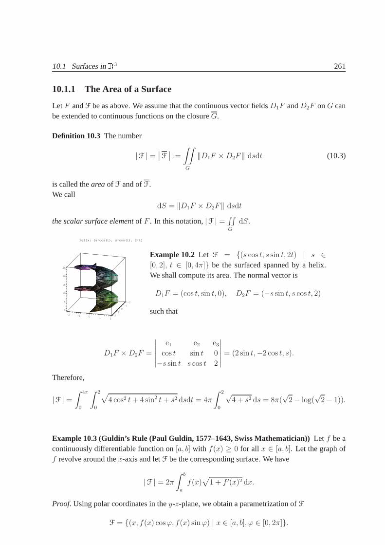
10.1 Surfaces inR3 261
10.1.1 The Area of a Surface
LetF andF be as above. We assume that the continuous vector fieldsD1F andD2F onG canbe extended to continuous functions on the closureG.
Definition 10.3 The number
|F | =∣∣F∣∣ :=
∫∫
G
‖D1F ×D2F‖ dsdt (10.3)
is called theareaof F and ofF.We call
dS = ‖D1F ×D2F‖ dsdt
the scalar surface elementof F . In this notation,|F | =∫∫G
dS.
-2-1
0
-2
0
5
1
-1
10
0
15
1
20
22
25
Helix: (s*cos(t), s*cos(t), 2*t)
Example 10.2 Let F = (s cos t, s sin t, 2t) | s ∈[0, 2], t ∈ [0, 4π] be the surfaced spanned by a helix.We shall compute its area. The normal vector is
D1F = (cos t, sin t, 0), D2F = (−s sin t, s cos t, 2)
such that
D1F ×D2F =
∣∣∣∣∣∣
e1 e2 e3
cos t sin t 0
−s sin t s cos t 2
∣∣∣∣∣∣= (2 sin t,−2 cos t, s).
Therefore,
|F | =∫ 4π
0
∫ 2
0
√4 cos2 t+ 4 sin2 t+ s2 dsdt = 4π
∫ 2
0
√4 + s2 ds = 8π(
√2− log(
√2− 1)).
Example 10.3 (Guldin’s Rule (Paul Guldin, 1577–1643, SwissMathematician)) Let f be acontinuously differentiable function on[a, b] with f(x) ≥ 0 for all x ∈ [a, b]. Let the graph off revolve around thex-axis and letF be the corresponding surface. We have
|F | = 2π
∫ b
a
f(x)√
1 + f ′(x)2 dx.
Proof. Using polar coordinates in they-z-plane, we obtain a parametrization ofF
F = (x, f(x) cosϕ, f(x) sinϕ) | x ∈ [a, b], ϕ ∈ [0, 2π].

262 10 Surface Integrals
We have
D1F = (1, f ′(x) cosϕ, f ′(x) sinϕ), D1F = (0,−f sinϕ, f cosϕ),
D1F ×D2F = (ff ′,−f cosϕ,−f sinϕ);
so thatdS = f(x)√
1 + f ′(x)2 dxdϕ. Hence
|F | =∫ b
a
∫ 2π
0
f(x)√
1 + f ′(x)2dϕ dx = 2π
∫ b
a
f(x)√
1 + f ′(x)2 dx.
10.2 Scalar Surface Integrals
Let F andF be as above, andf : F → R a continuous function on the compact subsetF ⊂ R3.
Definition 10.4 The number∫∫
F
f(~x) dS :=
∫∫
G
f(F (s, t)) ‖D1F (s, t)×D2(s, t)‖ dsdt
is called thescalar surface integral off onF.
10.2.1 Other Forms for dS
(a) Let the surfaceF be given as the graph of a functionF (x, y) = (x, y, f(x, y)), (x, y) ∈ G.Then, see Example 10.1,
dS =√
1 + f 2x + f 2
y dxdy.
(b) Let the surface be given implicitly asG(x, y, z) = 0. SupposeG is locally solvable forz ina neighborhood of some point(x0, y0, z0). Then the surface element (up to the sign) is given by
dS =
√F 2x + F 2
y + F 2z
|Fz |dxdy =
‖ gradF‖|Fz |
dxdy.
One checks thatDF1 ×DF2 = (Fx, Fy, Fz)/Fz.(c) If F is given byF (s, t) = (x(s, t), y(s, t), z(s, t)) we have
dS =√EG−H2 dsdt,
where
E = x2s + y2
s + z2s , G = x2
t + y2t + z2
t , H = xsxt + ysyt + zszt.

10.2 Scalar Surface Integrals 263
Indeed, using∥∥∥~a×~b
∥∥∥ = ‖~a‖∥∥∥~b∥∥∥ sinϕ andsin2 ϕ = 1− cos2 ϕ, whereϕ is the angle spanned
by~a and~b we get
EG−H2 = ‖D1F‖2 ‖D2F‖2 − (D1F ·D2F )2 = ‖D1F‖2 ‖D2F‖2 (1− cos2 ϕ)
= ‖D1F‖2 ‖D2F‖2 sin2 ϕ = ‖D1F ×D2F‖2
which proves the claim.
Example 10.4 (a) We give two different forms for the scalar surface element of a sphere. By(b), the spherex2 + y2 + z2 = R2 has surface element
dS =‖(2x, 2y, 2z)‖
2zdxdy =
R
zdxdy.
If
x = R cosϕ sinϑ, y = R sinϕ sinϑ, z = R cosϑ,
we obtain
D1 = Fϑ = R(cosϕ cosϑ, sinϕ cosϑ,− sin ϑ),
D2 = Fϕ = R(− sinϕ sinϑ, cosϕ sinϑ, 0),
D1 ×D2 = R2(cosϕ sin2 ϑ, sinϕ sin2 ϑ, sin ϑ cosϑ).
Hence,
dS = ‖D1 ×D2‖ dϑdϕ = R2 sinϑdϑdϕ.
(b) Riemann integral in R3 and surface integral over spheres.Let M = (x, y, z) ∈ R3 |ρ ≤ ‖(x, y, z)‖ ≤ R whereR > ρ ≥ 0. Let f : M → R be continuous. Let us denote thesphere of radiusr by Sr = (x, y, z) ∈ R3 | x2 + y2 + z2 = r2. Then
∫∫∫
M
f dxdydz =
∫ R
ρ
dr
∫∫
Sr
f(~x) dS
=
∫ R
ρ
r2
∫∫
S1
f(r~x) dS(~x)
dr.
Indeed, by the previous example, and by our knowledge of spherical coordinates(r, ϑ, ϕ).
dxdydz = r2 sinϑ dr dϑ dϕ = dr dSr.
On the other hand, on the unit sphereS1, dS = sinϑ dϑ dϕ such that
dxdydz = r2 dr dS
which establishes the second formula.

264 10 Surface Integrals
10.2.2 Physical Application
(a) If ρ(x, y, z) is the mass density on a surfaceF,∫∫F
ρ dS is the total mass ofF. The mass
center ofF has coordinates(xc, yc, zc) with
xc =1∫∫
F
ρ dS
∫∫
F
x ρ(x, y, z) dS,
and similarly foryc andzc.(b) If σ(~x) is a charge density on a surfaceF. Then
U(~y) =
∫∫
F
σ(~x)
‖~y − ~x‖ dS(~x), ~y 6∈ F
is the potential generated byF.
10.3 Surface Integrals
10.3.1 Orientation
We want to define the notion oforientationfor a regular surface. LetF be a regular (injective)surface with or without boundary. Then for every pointx0 ∈ F there exists the tangent planeEx0 ; the normal line toF atx0 is uniquely defined.However, a unit vector on the normal line can have two different directions.
Definition 10.5 (a) Let F be a surface as above. Aunit normal fieldto F is a continuousfunction~n : F → R3 with the following two properties for everyx0 ∈ F
(i) ~n(x0) is orthogonal to the tangent plane toF atx0.(ii) ‖~n(x0)‖ = 1.
(b) A regular surfaceF is calledorientable, if there exists a unit normal field onF.
SupposeF is an oriented, open, regular surface with piecewise smoothboundary∂F. LetF (s, t) be a parametrization ofF. We assume that the vector functionsF , DF1, andDF2 canbe extended to continuous functions onF. The unit normal vector is given by
~n = εD1F ×D2F
‖D1F ×D2F‖,
whereε = +1 or ε = −1 fixes theorientationof F. It turns out that for a regular surfaceFthere either exists exactly two unit normal fields or there isno such field. IfF is provided withan orientation we writeF+ for the pair(F, ~n). For F with the opposite orientation, we writeF−.
10.3 Surface Integrals 265
Examples of non-orientable surfaces are theMobius bandand thereal projective plane. Ana-lytically the Mobius band is given by
F (s, t) =
(1 + t cos s
2
)sin s(
1 + t cos s2
)cos s
t sin s2
, (s, t) ∈ [0, 2π]×
(−1
2,1
2
).
Definition 10.6 Let ~f : F → R3 be a continuous vector field onF. The number∫∫
F+
~f(~x) · ~ndS (10.4)
is called thesurface integral of the vector field~f onF+. We call
~dS = ~n dS = εD1F ×D2F dsdt
the surface elementof F.
Remark 10.1 (a) The surface integral is independent of the parametrization of F but dependson the orientation;
∫∫F+
~f· ~dS = −∫∫
F−
~f· ~dS.For, let(s, t) = (s(ξ, η), t(ξ, η)) be a new parametrization withF (s(ξ, η), t(ξ, η)) = G(ξ, η).Then the Jacobian is
dsdt =∂(s, t)
∂(ξ, η)= (sξtη − sηtξ) dξdη.
Further
D1G = D1F sξ +D2F tξ, D2G = D1F sη +D2Ftη,
so that using~x× ~x = 0, ~x× ~y = −~y × ~x
D1G×D2Gdξdη = (D1F sξ +D2F tξ)× (D1F sη +D2Ftη)dξdη,
= (sξtη − sηtξ)D1F ×D2Fdξdη
= D1F ×D2F dsdt.
(b) The scalar surface integral is a special case of the surface integral, namely∫∫f dS =
∫∫f~n·~n dS.
(c) Special cases. LetF be the graph of a functionf , F = (x, y, f(x, y)) | (x, y) ∈ C, then
~dS = ±(−fx,−fy, 1) dxdy.
If the surface is given implicitly byF (x, y, z) = 0 and it is locally solvable forz, then
~dS = ± gradF
Fzdxdy.

266 10 Surface Integrals
(d) Still another form of ~dS.∫∫
F
~f ~dS = ε
∫∫
G
f(F (s, t)) · (D1F ×D2F ) dsdt
~f(F (s, t)) · (D1F ×D2F ) =
∣∣∣∣∣∣
f1(F (s, t)) f2(F (s, t)) f3(F (s, t))
xs(s, t) ys(s, t) zs(s, t)
xt(s, t) yt(s, t) zt(s, t)
∣∣∣∣∣∣. (10.5)
(e) Again another notation. Computing the previous determinant or the determinant (10.1)explicitely we have
~f ·(D1F×D2F ) = f1
∣∣∣∣ys zsyt zt
∣∣∣∣+f2
∣∣∣∣zs xszt xt
∣∣∣∣+f3
∣∣∣∣xs ysxt yt
∣∣∣∣ = f1∂(y, z)
∂(s, t)+f2
∂(z, x)
∂(s, t)+f3
∂(x, y)
∂(s, t).
Hence,
~dS = εD1F ×D2F dsdt = ε
(∂(y, z)
∂(s, t)dsdt,
∂(z, x)
∂(s, t)dsdt,
∂(x, y)
∂(s, t)dsdt
)
~dS = ε ( dydz, dzdx, dxdy) .
Therefore we can write∫∫
F
~f · ~dS =
∫∫
F
(f1 dydz + f2 dzdx + f3 dxdy) .
In this setting∫∫
F
f1 dydz =
∫∫
F
(f1, 0, 0) · ~dS = ±∫∫
G
f1(F (s, t))∂(y, z)
∂(s, t)dsdt.
Sometimes one uses~dS = (cos(~n, e1), cos(~n, e2), cos(~n, e3)) dS,
sincecos(~n, ei) = ~n·ei = ni and ~dS = ~n dS.Note that we have surface integrals in the last two lines, notordinary double integrals sinceFis a surface inR3 andf1 = f1(x, y, z) can also depend onx.The physical meaning of
∫∫F~f · ~dS is the flow of the vector field~f through the surfaceF. The
flow is (locally) positive if~n and ~f are on the same side of the tangent plane toF and negativein the other case.
Example 10.5 (a) Compute the surface integral∫∫
F+
f dzdx
of f(x, y, z) = x2yz whereF is the graph ofg(x, y) = x2 + y over the unit squareG =
[0, 1]× [0, 1] with the downward directed unit normal field.

10.3 Surface Integrals 267
By Remark 10.1 (c)~dS = (gx, gy,−1) dxdy = (2x, 1,−1) dxdy.
Hence∫∫
F+
f dzdx =
∫∫
F+
(0, f, 0) · ~dS
= (R)
∫∫
G
x2y(x2 + y) dxdy =
∫ 1
0
dx
∫ 1
0
(x4y + x2y2) dy =19
90.
x
y
z
R
R
(b) LetG denote the upper half ball of radiusR in R3:
G = (x, y, z) | x2 + y2 + z2 ≤ R2, z ≥ 0,
and letF be the boundary ofG with the orientation of theouter normal. ThenF consists of the upper half sphereF1
F1 = (x, y,√R2 − x2 − y2) | x2 + y2 ≤ R2, z = g(x, y) =
√R2 − x2 − y2,
with the upper orientation of the unit normal field and of the discF2 in thex-y-plane
F2 = (x, y, 0) | x2 + y2 ≤ R2, z = g(x, y) = 0,
with the downward directed normal. Let~f(x, y, z) = (ax, by, cz). We want to compute∫∫
F+
~f · ~dS.
By Remark 10.1 (c), the surface element of the half-sphereF1 is ~dS = 1z(x, y, z) dxdy. Hence
I1 =
∫∫
F1+
~f · ~dS =
∫∫
BR
(ax, by, cz) · 1z(x, y, z) dxdy =
∫∫
BR
1
z(ax2 + by2 + cz2)
∣∣∣∣z=g(x,y)
dxdy.
Using polar coordinatesx = r cosϕ, y = r sinϕ, r ∈ [0, R], andz =√R2 − x2 − y2 =√
R2 − r2 we get
I1 =
∫ 2π
0
dϕ
∫ R
0
ar2 cos2 ϕ+ br2 sin2 ϕ+ c(R2 − r2)√R2 − r2
rdr.
Noting∫ 2π
0sin2 ϕdϕ =
∫ 2π
0cos2 ϕdϕ = π we continue
I1 = π
∫ R
0
(ar3
√R2 − r2
+br3
√R2 − r2
+ 2cr√R2 − r2
)dr.

268 10 Surface Integrals
Usingr = R sin t, dr = R cos t dt we have
∫ R
0
r3
√R2 − r2
dr =
∫ π2
0
R3 sin3 tR cos t dt
R√
1− sin2 t= R3
∫ π2
0
sin3 t dt =2
3R3.
Hence,
I1 =2π
3R3(a + b) + πc
∫ R
0
(R2 − r2)12 d(r2)
=2π
3R3(a + b) + πc
[−2
3(R2 − r2)
32
∣∣∣∣R
0
=2π
3R3(a + b+ c).
In case of the discF2 we havez = f(x, y) = 0, such thatfx = fy = 0 and
~dS = (0, 0,−1) dxdy
by Remark 10.1 (c). Hence∫∫
F2+
~f · ~dS =
∫∫
BR
(ax, by, cz) · (0, 0,−1) dxdy = −c∫∫
BR
z dxdy =z=0
0.
Hence, ∫∫
F
(ax, by, cz) · ~dS =2π
3R3(a+ b+ c).
10.4 Gauß’ Divergence Theorem
The aim is to generalize the fundamental theorem of calculusto higher dimensions:∫ b
a
f ′(x) dx = f(b)− f(a).
Note thata andb form the boundary of the segment[a, b]. There are three possibilities to do this
∫∫∫G
g dxdydz =⇒∫∫
(∂G)+
~f· ~dS Gauß’ theorem inR3,
∫∫G
g dxdy =⇒∫
(∂G)+
~f·d~x Green’s theorem inR2,
∫∫F+
~g· ~dS =⇒∫
(∂G)+
~f·d~x Stokes’ theorem .
LetG ⊂ R3 be a bounded domain (open, connected) such that its boundaryF = ∂G satisfiesthe following assumptions:
1. F is a union of regular, orientable surfacesFi. The parametrizationFi(s, t), (s, t) ∈ Ci,of Fi as well asD1Fi andD2Fi are continuous vector functions onCi; Ci is a domain inR2.
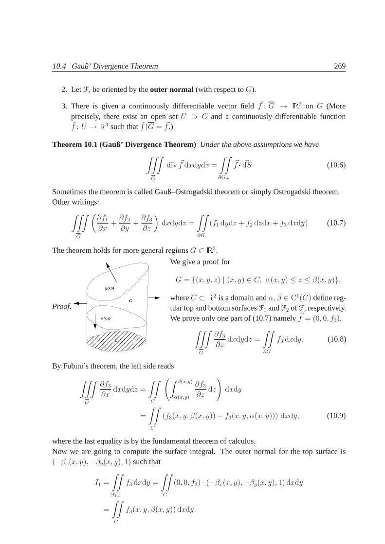
10.4 Gauß’ Divergence Theorem 269
2. LetFi be oriented by theouter normal (with respect toG).
3. There is given a continuously differentiable vector field~f : G → R3 on G (Moreprecisely, there exist an open setU ⊃ G and a continuously differentiable functionf : U → R3 such thatfG = ~f .)
Theorem 10.1 (Gauß’ Divergence Theorem)Under the above assumptions we have∫∫∫
G
div ~f dxdydz =
∫∫
∂G+
~f· ~dS (10.6)
Sometimes the theorem is called Gauß–Ostrogadski theorem or simply Ostrogadski theorem.Other writings:
∫∫∫
G
(∂f1
∂x+∂f2
∂y+∂f3
∂z
)dxdydz =
∫∫
∂G
(f1 dydz + f2 dzdx + f3 dxdy) (10.7)
The theorem holds for more general regionsG ⊂ R3.
Proof.
C
α
β(x,y)
(x,y)
G
We give a proof for
G = (x, y, z) | (x, y) ∈ C, α(x, y) ≤ z ≤ β(x, y),
whereC ⊂ R2 is a domain andα, β ∈ C1(C) define reg-ular top and bottom surfacesF1 andF2 of F, respectively.We prove only one part of (10.7) namely~f = (0, 0, f3).
∫∫∫
G
∂f3
∂zdxdydz =
∫∫
∂G
f3 dxdy. (10.8)
By Fubini’s theorem, the left side reads
∫∫∫
G
∂f3
∂xdxdydz =
∫∫
C
(∫ β(x,y)
α(x,y)
∂f3
∂zdz
)dxdy
=
∫∫
C
(f3(x, y, β(x, y))− f3(x, y, α(x, y))) dxdy, (10.9)
where the last equality is by the fundamental theorem of calculus.Now we are going to compute the surface integral. The outer normal for the top surface is(−βx(x, y),−βy(x, y), 1) such that
I1 =
∫∫
F1+
f3 dxdy =
∫∫
C
(0, 0, f3) · (−βx(x, y),−βy(x, y), 1) dxdy
=
∫∫
C
f3(x, y, β(x, y)) dxdy.

270 10 Surface Integrals
Since the bottom surfaceF2 is oriented downward, the outer normal is(αx(x, y), αy(x, y),−1)
such that
I2 =
∫∫
F2+
f3 dxdy = −∫∫
C
f3(x, y, α(x, y)) dxdy.
Finally, the shellF3 is parametrized by an angleϕ andz:
F3 = (r(ϕ) cosϕ, r(ϕ) sinϕ, z) | α(x, y) ≤ z ≤ β(x, y), ϕ ∈ [0, 2π].
SinceD2F = (0, 0, 1), the normal vector is orthogonal to thez-axis,~n = (n1, n2, 0). Therefore,
I3 =
∫∫
F3+
f3 dxdy =
∫∫
F3+
(0, 0, f3) · (n1, n2, 0) dS = 0.
ComparingI1 + I2 + I3 with (10.9) proves the theorem in this special case.
Remarks 10.2 (a) Gauß’ divergence theorem can be used to compute the volume of the domainG ⊂ R3. Suppose the boundary∂G of G has the orientation of the outer normal. Then
v(G) =
∫∫
∂G
x dydz =
∫∫
∂G
y dzdx =
∫∫
∂G
z dxdy.
(b) Applying the mean value theorem to the left-hand side of Gauß’ formula we have for anybounded regionG containingx0
div ~f(x0 + h)
∫∫∫
G
dxdydz = div ~f(x0 + h)v(G) =
∫∫
∂G+
~f· ~dS,
whereh is a small vector. The integral on the left is the volumev(G). Hence
div ~f(x0) = limG→x0
1
v(G)
∫∫
∂G+
~f· ~dS = limε→0
14πε3
3
∫∫
Sε(x0)+
~f· ~dS,
where the regionG tends tox0. In the second formula, we have chosenG = Bε(x0) the openball of radiusε with centerx0. The right hand side can be thought as to be thesource densityofthe field ~f . In particular, the right side gives a basis independent description of div ~f .
Example 10.6 We want to compute the surface integral from Example 10.5 (b)using Gauß’theorem:∫∫
F+
~f· ~dS =
∫∫∫
C
div f dxdydz =
∫∫∫
x2+y2+z2≤R2, z≥0
(a+ b+ c) dxdydz =2πR3
3(a + b+ c).

10.4 Gauß’ Divergence Theorem 271
Gauß’ divergence theorem which play an important role in partial differential equations.Recall (Proposition 7.9 (Prop. 8.9)) that thedirectional derivativeof a functionv : U → R,U ⊂ Rn, atx0 in the direction of the unit vector~n is given byD~nf(x0) = grad f(x0)·~n.Notation. Let U ⊂ R3 be open andF+ ⊂ U be an oriented, regular open surface with the unitnormal vector~n(x0) atx0 ∈ F. Let g : U → R be differentiable.Then
∂g
∂~n(x0) = grad g(x0)·~n(x0) (10.10)
is called thenormal derivativeof g onF+ atx0.
Proposition 10.2 LetG be a region as in Gauß’ theorem, the boundary∂G is oriented with theouter normal,u, v are twice continuously differentiable on an open setU withG ⊂ U . Then wehave Green’s identities:
∫∫∫
G
∇(u)·∇(v) dxdydz =
∫∫
∂G
u∂v
∂~ndS −
∫∫∫
G
u∆(v) dxdydz, (10.11)
∫∫∫
G
(u∆(v)− v∆(u)) dxdydz =
∫∫
∂G
(u∂v
∂~n− v ∂u
∂~n
)dS, (10.12)
∫∫∫
G
∆(u) dxdydz =
∫∫
∂G
∂u
∂~ndS. (10.13)
Proof. Putf = u∇(v). Then by nabla calculus
div f = ∇(u∇v) = ∇(u) · ∇(v) + u∇·(∇v)= gradu· grad v + u∆(v).
Applying Gauß’ theorem, we obtain∫∫∫
G
div f dxdydz =
∫∫∫
G
( gradu· grad v) dxdydz +
∫∫∫
G
u∆(v) dxdydz
=
∫∫
∂G
u grad v · ~n dS =
∫∫
∂G
u∂v
∂~ndS.
This proves Green’s first identity. Changing the role ofu andv and taking the difference, weobtain the second formula.Insertingv = −1 into (10.12) we get (10.13).
Application to Laplace equation
Let u1 and u2 be functions onG with ∆u1 = ∆u2, which coincide on the boundary∂G,u1(x) = u2(x) for all x ∈ ∂G. Thenu1 ≡ u2 in G.
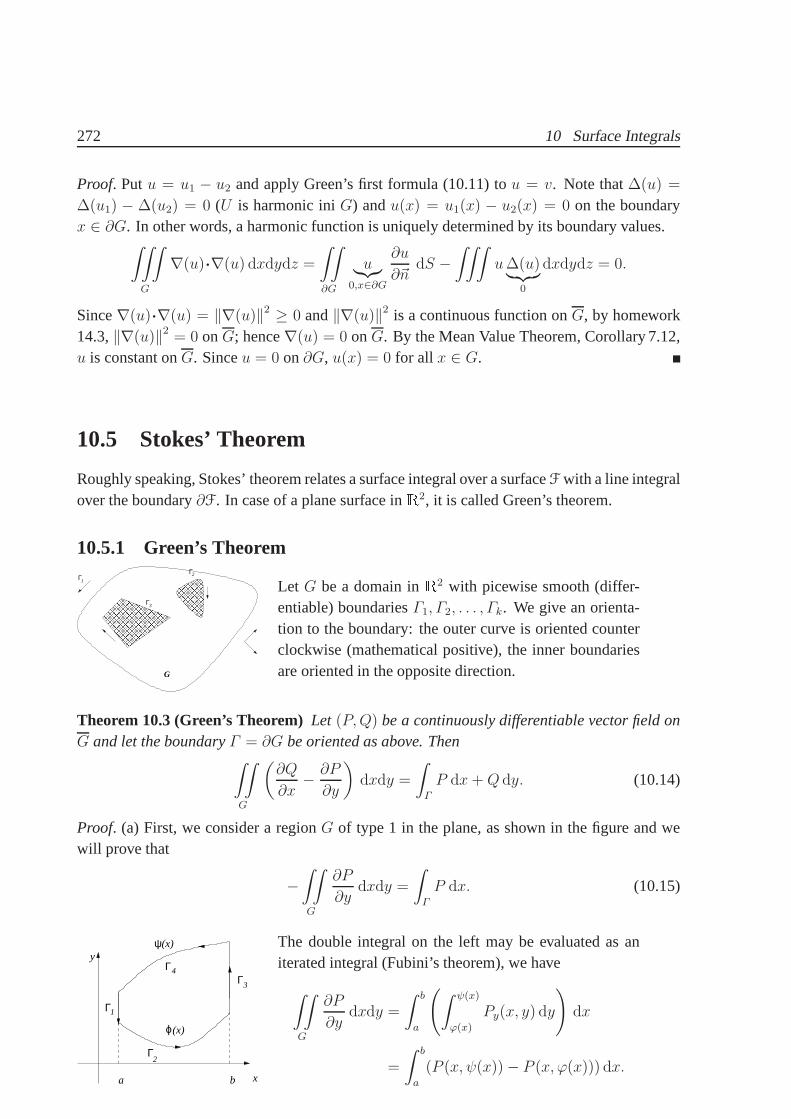
272 10 Surface Integrals
Proof. Putu = u1 − u2 and apply Green’s first formula (10.11) tou = v. Note that∆(u) =
∆(u1) − ∆(u2) = 0 (U is harmonic iniG) andu(x) = u1(x) − u2(x) = 0 on the boundaryx ∈ ∂G. In other words, a harmonic function is uniquely determinedby its boundary values.
∫∫∫
G
∇(u)·∇(u) dxdydz =
∫∫
∂G
u︸︷︷︸0,x∈∂G
∂u
∂~ndS −
∫∫∫u∆(u)︸ ︷︷ ︸
0
dxdydz = 0.
Since∇(u)·∇(u) = ‖∇(u)‖2 ≥ 0 and‖∇(u)‖2 is a continuous function onG, by homework14.3,‖∇(u)‖2 = 0 onG; hence∇(u) = 0 onG. By the Mean Value Theorem, Corollary 7.12,u is constant onG. Sinceu = 0 on∂G, u(x) = 0 for all x ∈ G.
10.5 Stokes’ Theorem
Roughly speaking, Stokes’ theorem relates a surface integral over a surfaceF with a line integralover the boundary∂F. In case of a plane surface inR2, it is called Green’s theorem.
10.5.1 Green’s Theorem
Γ
Γ
Γ2
3
1
G
Let G be a domain inR2 with picewise smooth (differ-entiable) boundariesΓ1, Γ2, . . . , Γk. We give an orienta-tion to the boundary: the outer curve is oriented counterclockwise (mathematical positive), the inner boundariesare oriented in the opposite direction.
Theorem 10.3 (Green’s Theorem)Let (P,Q) be a continuously differentiable vector field onG and let the boundaryΓ = ∂G be oriented as above. Then
∫∫
G
(∂Q
∂x− ∂P
∂y
)dxdy =
∫
Γ
P dx+Q dy. (10.14)
Proof. (a) First, we consider a regionG of type 1 in the plane, as shown in the figure and wewill prove that
−∫∫
G
∂P
∂ydxdy =
∫
Γ
P dx. (10.15)
(x)ψ
(x)ϕ
4
3
Γ2
a b x
y
Γ
ΓΓ
1
The double integral on the left may be evaluated as aniterated integral (Fubini’s theorem), we have
∫∫
G
∂P
∂ydxdy =
∫ b
a
(∫ ψ(x)
ϕ(x)
Py(x, y) dy
)dx
=
∫ b
a
(P (x, ψ(x))− P (x, ϕ(x))) dx.

10.5 Stokes’ Theorem 273
The latter equality is due to the fundamental theorem of calculus. To compute the line integral,we parametrize the four parts ofΓ in a natural way:
−Γ1, ~x1(t) = (a, t), t ∈ [ϕ(a), ψ(a)], dx = 0, dy = dt,
Γ2, ~x2(t) = (t, ϕ(t)), t ∈ [a, b], dx = dt, dy = ϕ′(t) dt,
Γ3, ~x3(t) = (b, t), t ∈ [ϕ(b), ψ(b)], dx = 0, dy = dt,
−Γ4, ~x4(t) = (t, ψ(t)), t ∈ [a, b], dx = dt, dy = ψ′(t) dt.
Sincedx = 0 onΓ1 andΓ3 we are left with the line integrals overΓ2 andΓ4:∫
Γ
P dx =
∫ b
a
P (t, ϕ(t)) dt−∫ b
a
P (t, ψ(t)) dt
Let us prove the second part,−∫∫G
∂Q∂x
dxdy =∫ΓQ dy. Using Proposition 7.24 we have
∫ ψ(x)
ϕ(x)
∂
∂xQ(x, y) dy =
d
dx
(∫ ψ(x)
ϕ(x)
Q(x, y) dy
)− ψ′(x)Q(x, ψ(x)) + ϕ′(x)Q(x, ϕ(x)).
Inserting this into∫∫G
∂Q∂x
dxdy =∫ ba
(∫ ψ(x)
ϕ(x)∂Q∂x
dy)
dx, we get
∫∫
G
∂Q
∂xdxdy =
∫ b
a
(d
dx
(∫ ψ(x)
ϕ(x)
Q(x, y) dy
)− ψ′(x)Q(x, ψ(x)) + ϕ′(x)Q(x, ϕ(x))
)dx
=
∫ ψ(b)
ϕ(b)
Q(b, y) dy −∫ ψ(a)
ϕ(a)
Q(a, y) dy −∫ b
a
Q(x, ψ(x))ψ′(x) dx+ (10.16)
+
∫ b
a
Q(x, ϕ(x))ϕ′(x) dx. (10.17)
We compute the line integrals:
−∫
−Γ1
Q dy = −∫ ψ(a)
ϕ(a)
Q(a, y) dy,
∫
Γ3
Q dy =
∫ ψ(b)
ϕ(b)
Q(b, y) dy.
Further,∫
Γ2
Q dy =
∫ b
a
Q(t, ϕ(t))ϕ′(t) dt, −∫
−Γ4
Q dy = −∫ b
a
Q(t, ψ(t))ψ′(t) dt.
Adding up these integrals and comparing the result with (10.17), the proof for type 1 regions iscomplete.
(x)ϕ (x)ψΓ2
Γ3
x
y
Γ1
Γ4
type 2
type 2
type 2
type 1

274 10 Surface Integrals
Exactly in the same way, we can prove that ifG is a type 2 region then (10.14) holds.
(b) Breaking a regionG up into smaller regions, each of which is both of type 1 and 2, Green’stheorem is valid forG. The line integrals along the inner boundary cancel leavingthe lineintegral around the boundary ofG.
(c) If the region has a hole, one can split it into two simply connected regions, for whichGreen’s theorem is valid by the arguments of (b).
Application: Area of a Region
If Γ is a curve which bounds a regionG, then the area ofG is A =∫Γ(1 − α)x dy − αy dx
whereα ∈ R is arbitrary, in particular,
A =1
2
∫
Γ
x dy − y dx =
∫
Γ
x dy = −∫
Γ
y dx. (10.18)
Proof. ChoosingQ = (1− α)x, P = −αy one has
A =
∫∫
G
dxdy =
∫∫
G
((1− α)− (−α)) dxdy =
∫∫
G
(Qx − Py) dxdy =
∫
Γ
P dx+Q dy
= −α∫
Γ
y dx+ (1− α)
∫
Γ
x dy.
Insertingα = 0, α = 1, andα = 12
yields the assertion.
Example 10.7 Find the area bounded by the ellipseΓ :x2
a2+y2
b2= 1. We parametrizeΓ by
~x(t) = (a cos t, b sin t), t ∈ [0, 2π], ~x(t) = (−a sin t, b cos t). Then (10.18) gives
A =1
2
∫ 2π
0
a cos t b sin t dt− b sin t(−a sin t) dt =1
2
∫ 2π
0
ab dt = πab.
10.5.2 Stokes’ Theorem
Conventions: LetF+ be a regular, oriented surface. LetΓ = ∂F+ be the boundary ofF with theinduced orientation:the orientation of the surface (normal vector) together with the orientationof the boundary form a right-oriented screw. A second way to get the induced orientation:sitting in the arrowhead of the unit normal vector to the surface, the boundary curve has counterclockwise orientation.
Theorem 10.4 (Stokes’ theorem)Let F+ be a smooth regular oriented surface with aparametrizationF ∈ C2(G) andG is a plane region to which Green’s theorem applies. Let

10.5 Stokes’ Theorem 275
Γ = ∂F be the boundary with the above orientation. Further, let~f be a continuously differen-tiable vector field onF.Then we have
∫∫
F+
curl ~f· ~dS =
∫
∂F+
~f· d~x. (10.19)
This can also be written as∫∫
F+
(∂f3
∂y− ∂f2
∂z
)dydz+
(∂f1
∂z− ∂f3
∂x
)dzdx+
(∂f2
∂x− ∂f1
∂y
)dxdy =
∫
Γ
f1 dx+f2 dy+f3 dz.
Proof. Main idea: Reduction to Green’s theorem. Since both sides of the equation are additivewith respect to the vector field~f , it suffices to proof the statement for the vector fields(f1, 0, 0),(0, f2, 0), and (0, 0, f3). We show the theorem for~f = (f, 0, 0), the other cases are quiteanalogous: ∫∫
F
(∂f
∂zdzdx − ∂f
∂ydxdy
)=
∫
∂F
f dx.
Let F (u, v), u, v ∈ G be the parametrization of the surfaceF. Then
dx =∂x
∂udu+
∂x
∂vdv,
such that the line integral on the right reads withP (u, v) = f(x(u, v), y(u, v), z(u, v)) ∂x∂u
(u, v)
andQ(u, v) = f ∂x∂v
.
∫
∂F
f dx =
∫
∂G
f xu du+ f xv dv =
∫
∂G
P du+Q dv =Green′s th.
∫∫
G
(−∂P∂v
+∂Q
∂u
)du dv
=
∫∫
G
−(fuxu + f xvu) + (fuxv + f xuv) du dv =
∫∫
G
−fvxu + fuxv du dv
=
∫∫
G
−(fx xv + fy yv + fz zv)xu + (fx xu + fy yu + fz zu)xv du dv
=
∫∫
G
(−fy(xuyv − xvyu) + fz(zuxv − zvxu)) du dv
=
∫∫
G
(−fy
∂(x, y)
∂(u, v)+ fz
∂(z, x)
∂(u, v)
)du dv =
∫∫
F
−fy dxdy + fz dzdx.
This completes the proof.
Remark 10.3 (a) Green’s theorem is a special case withF = G× 0, ~n = (0, 0, 1) (orienta-tion) and~f = (P,Q, 0).

276 10 Surface Integrals
(b) The right side of (10.19) is called thecirculation of the vector field~f over the closed curveΓ . Now let ~x0 ∈ F be fixed and consider smaller and smaller neighborhoodsF0+ of ~x0 withboundariesΓ0. By Stokes’ theorem and by the Mean Value Theorem of integration,
∫
Γ0
~f d~x =
∫∫
F0
curl ~f·~n dS = curl ~f(x0)~n(x0) area (F0).
Hence,
curl ~f(x0)·~n(x0) = limF0→x0
∫∂F0
~f d~x
|F0 |.
We call curl ~f(x0) · ~n(x0) the infinitesimal circulationof the vector field~f atx0 correspondingto the unit normal vector~n.(c) Stokes’ theorem then says that the integral over the infinitesimal circulation of a vector field~f corresponding to the unit normal vector~n overF equals the circulation of the vector fieldalong the boundary ofF.
Path Independence of Line Integrals
We are going complete the proof of Proposition 8.3 and show that for a
simplyconnected regionG ⊂ R3 anda twice continuously differentiable vector field~f withcurl ~f = 0 for all x ∈ G
the vector field~f is conservative.Proof. Indeed, letΓ be a closed, regular, piecewise differentiable curveΓ ⊂ G and letΓ be thethe boundary of a smooth regular oriented surfaceF+, Γ = ∂F+ such thatΓ has the inducedorientation. Insertingcurl ~f = 0 into Stokes’ theorem gives
∫∫
F+
curl f· ~dS = 0 =
∫
Γ
~f· d~x;
the line integral is path independent and hence,~f is conservative. Note that the region must besimply connected; otherwise its in general impossible to find F with boundaryΓ .
10.5.3 Vector Potential and the Inverse Problem of Vector Analysis
Let ~f be a continuously differentiable vector field on thesimply connectedregionG ⊂ R3.
Definition 10.7 The vector field~f onG is called asource-freefield (solenoidal field) if thereexists a vector field~g onG with ~f = curl~g. Then~g is called thevector potentialto ~f .
Theorem 10.5 ~f is source-free if and only ifdiv ~f = 0.

10.5 Stokes’ Theorem 277
Proof. (a) If ~f = curl~g then div ~f = div ( curl~g) = 0.(b) To simplify notations, we skip the arrows. We explicitlyconstruct a vector potentialg to fwith g = (g1, g2, 0) and curl g = f . This means
f1 = −∂g2
∂z,
f2 =∂g1
∂z,
f3 =∂g2
∂x− ∂g1
∂y.
Integrating the first two equations, we obtain
g2 = −∫ z
z0
f1(x, y, t) dt+ h(x, y),
g1 =
∫ z
z0
f2(x, y, t) dt,
whereh(x, y) is the integration constant, not depending onz. Inserting this into the third equa-tion, we obtain
∂g2
∂x− ∂g1
∂y= −
∫ z
z0
∂f1
∂x(x, y, t) dt+ hx(x, y)−
∫ z
z0
∂f2
∂y(x, y, t) dt
= −∫ z
z0
(∂f1
∂x+∂f2
∂y
)dt+ hx
=div f=0
∫ z
z0
∂f3
∂z(x, y, t) dt+ hx
f3(x, y, z) = f3(x, y, z)− f3(x, y, z0) + hx(x, y).
This yields, hx(x, y) = f3(x, y, z0). Integration with respect tox finally givesh(x, y) =
∫ xx0f3(t, y, z0) dt; the third equation is satisfied andcurl g = f .
Remarks 10.4 (a) The proof of second direction is a constructive one; you can use this methodto calculate a vector potential explicitly. You can also tryanother ansatz, sayg = (0, g2, g3) org = (g1, 0, g3).(b) If g is a vector potential forf andU ∈ C2(G), theng = g+ gradU is also a vector potentialfor f . Indeed
curl g = curl g + curl gradU = f.
The Inverse Problem of Vector Analysis
Let h be a function and~a be a vector field onG; both continuously differentiable.Problem: Does there exist a vector field~f such that
div ~f = h and curl ~f = ~a.

278 10 Surface Integrals
Proposition 10.6 The above problem has a solution if and only ifdiv~a = 0.
Proof. The condition is necessary sincediv~a = div curl ~f = 0. We skip the vector arrows.For the other direction we use the ansatzf = r + s with
curl r = 0, div r = h, (10.20)
curl s = a, div s = 0. (10.21)
Since curl r = 0, by Proposition 8.3 there exists a potentialU with r = gradU . Thencurl r = 0 and div r = div gradU = ∆(U). Hence (10.20) is satisfied if and only ifr = gradU and∆(U) = h.Sincediv a = 0 by asssumption, there exists a vector potentialg such thatcurl g = a. Letϕ betwice continuously differentiable onG and sets = g + gradϕ. Then curl s = curl g = a anddiv s = div g+ div gradϕ = div g+ ∆(ϕ). Hence,div s = 0 if and only if ∆(ϕ) = − div g.Both equations∆(U) = h and∆(ϕ) = − div g are so called Poisson equations which can besolved within the theory of partial differential equations(PDE).
The inverse problem hasnot a unique solution. Choose a harmonic functionψ, ∆(ψ) = 0 andputf1 = f + gradψ. Then
div f1 = div f + div gradψ = div f + ∆(ψ) = div f = h,
curl f1 = curl f + curl gradψ = curl f = a.

Chapter 11
Differential Forms on Rn
We show that Gauß’, Green’s and Stokes’ theorems are three cases of a “general” theorem whichis also named after Stokes. The simple formula now reads
∫c
dω =∫∂cω. The appearance of
the Jacobian in the change of variable theorem will become clear. We formulate the Poincarelemma.Good references are [Spi65], [AF01], and [vW81].
11.1 The Exterior AlgebraΛ(Rn)
Although we are working with the ground fieldR all constructions make sense for arbitraryfieldsK, in particular,K = C. Let e1, . . . , en be the standard basis ofRn; for h ∈ Rn wewrite h = (h1, . . . , hn) with respect to the standard basis,h =
∑i hiei.
11.1.1 The Dual Vector SpaceV ∗
The interplay between a normed spaceE and its dual spaceE ′ forms the basis offunctionalanalysis. We start with the definition of the (algebraic) dual.
Definition 11.1 Let V be a linear space. Thedual vector spaceV ∗ to V is the set of all linearfunctionalsf : V → R,
V ∗ = f : V → R | f is linear.
It turns out thatV ∗ is again a linear space if we introduce addition and scalar multiples in thenatural way. Forf, g ∈ V ∗, α ∈ R put
(f + g)(v) := f(v) + g(v), (αf)(v) := αf(v).
Theevaluationof f ∈ V ∗ onv ∈ V is sometimes denoted by
f(v) = 〈f , v〉 ∈ K.279

280 11 Differential Forms onRn
In this case, the brackets denote thedual pairingbetweenV ∗ andV . By definition, the pairingis linear in both components. That is, for allv, w ∈ V and for allλ, µ ∈ R
〈λf + µg , v〉 = λ 〈f , v〉+ µ 〈g , v〉 ,〈f , λv + µw〉 = λ 〈f , v〉+ µ 〈f , w〉 .
Example 11.1 (a) LetV = Rn with the above standard basis. Fori = 1, . . . , n define theithcoordinate functionaldxi : Rn → R by
dxi(h) = dxi(h1, . . . , hn) = hi, h ∈ Rn.
The functionaldxi associates to each vectorh ∈ Rn its ith coordinatehi. The functionaldxi isindeed linear since for allv, w ∈ Rn andα, β ∈ R, dxi(αv+βw) = (αv+βw)i = αvi+βwi =
α dxi(v) + β dxi(w).
The linear space(Rn)∗ has also dimensionn. We will show that dx1, dx2, . . . , dxn is abasis of(Rn)∗. We call it thedual basisof to e1, . . . , en. Using the Kronecker symbol theevaluation ofdxi on ej reads as follows
dxi(ej) = δij , i, j = 1, . . . , n.
dx1, dx2, . . . , dxn generatesV ∗. Indeed, letf ∈ V ∗. Thenf =∑n
i=1 f(ei) dxi since bothcoincide for allh ∈ V :
n∑
i=1
f(ei) dxi(h) =
n∑
i=1
f(ei) hi =f homog.
∑
i
f(hiei) = f
(∑
i
hiei
)= f(h).
In Propostition 11.1 below, we will see that dx1, . . . , dxn is not only generating but linearlyindependent.
(b) If V = C([0, 1]), the continuous functions on[0, 1] andα is an increasing on[0, 1] function,then the Riemann-Stieltjes integral
ϕα(f) =
∫ 1
0
f dα, f ∈ V
defines a linear functionalϕα onV .If a ∈ [0, 1],
δa(f) = f(a), f ∈ V
defines theevaluation functionalof f ata. In casea = 0 this is Dirac’sδ-functional playing animportant role in the theory of distributions (generalizedfunctions).
(c) Let a ∈ Rn. Then〈a , x〉 =∑n
i=1 aixi, x ∈ Rn defines a linear functional onRn. By (a)this is already the most general form of a linear functional onRn.

11.1 The Exterior AlgebraΛ(Rn) 281
Definition 11.2 Let k ∈ N. An alternating (or skew-symmetric) multilinear form of degreek onRn, a k-form for short, is a mappingω : Rn × · · · × Rn → R, k factorsRn, which ismultilinearandskew-symmetric, i. e.
MULT ω(· · · , αvi + βwi, · · · ) = αω(· · · , vi, · · · ) + βω(· · · , wi, · · · ), (11.1)
SKEW ω(· · · , vi, · · · , vj , · · · ) = −ω(· · · , vj, · · · , vi, · · · ), i, j = 1, . . . , k, i 6= j, (11.2)
for all vectorsv1, v2, . . . , vk, wi ∈ Rn.
We denote the linear space of allk-forms onRn by Λk(Rn) with the conventionΛ0(Rn) = R.In casek = 1 property (11.2) is an empty condition such thatΛ1(Rn) = (Rn)∗ is just the dualspace.Let f1, . . . , fk ∈ (Rn)∗ be linear functionals onRn. Then we define thek-formf1∧ · · · ∧fk ∈ Λk(Rn) (read: “f1 wedgef2 . . . wedgefk”) as follows
f1∧ · · · ∧fk(h1, . . . , hk) =
∣∣∣∣∣∣∣
f1(h1) · · · f1(hk)...
...fk(h1) · · · fk(hk)
∣∣∣∣∣∣∣(11.3)
In particular, leti1, . . . , ik ∈ 1, . . . , n be fixed and choosefj = dxij , j = 1, . . . , k. Then
dxi1∧ · · · ∧ dxik(h1, . . . , hk) =
∣∣∣∣∣∣∣
h1i1 · · · hki1...
...h1ik · · · hkik
∣∣∣∣∣∣∣
f1∧ · · · ∧fk is indeed ak-form since thefi are linear, the determinant is multilinear
∣∣∣∣∣∣
λa + µa′ b c
λd+ µd′ e f
λg + µg′ h i
∣∣∣∣∣∣= λ
∣∣∣∣∣∣
a b c
d e f
g h i
∣∣∣∣∣∣+ µ
∣∣∣∣∣∣
a′ b c
d′ e f
g′ h i
∣∣∣∣∣∣,
and skew-symmetric ∣∣∣∣∣∣
a b c
d e f
g h i
∣∣∣∣∣∣= −
∣∣∣∣∣∣
b a c
e d f
h g i
∣∣∣∣∣∣.
For example, lety = (y1, . . . , yn), z = (z1, . . . , zn) ∈ Rn,
dx3∧ dx1(y, z) =
∣∣∣∣y3 z3y1 z1
∣∣∣∣ = y3z1 − y1z3.
If fr = fs = f for somer 6= s, we havef1∧ · · · ∧f∧ · · · ∧f∧ · · · ∧fk = 0 since determinantswith identical rows vanish. Also, for anyω ∈ Λk(Rn),
ω(h1, . . . , h, . . . , h, . . . , hk) = 0, h1, . . . , hk, h ∈ Rn
since the defining determinant has two identical columns.

282 11 Differential Forms onRn
Proposition 11.1 For k ≤ n thek-forms dxi1∧ · · · ∧ dxik | 1 ≤ i1 < i2 < · · · < ik ≤ nform a basis of the vector spaceΛk(Rn). A k-form withk > n is identically zero. We have
dimΛk(Rn) =
(n
k
).
Proof. Any k-formω is uniquely determined by its values on thek-tuple of vectors(ei1 , . . . , eik)with 1 ≤ i1 < i2 < · · · < ik ≤ n. Indeed, using skew-symmetry ofω, we knowω on all k-tuples of basis vectors; using linearity in each component,we getω on all k-tuples of vectors.This shows that thedxi1∧ · · · ∧ dxik with 1 ≤ i1 < i2 < · · · < ik ≤ n generate the linear spaceΛk(Rn). We make this precise in casek = 2. With y =
∑i yiei, z =
∑j zjej we have by
linearity and skew-symmetry ofω
ω(y, z) =n∑
i,j=1
yizjω(ei, ej) =SKEW
∑
1≤i<j≤n(yizj − yjzi)ω(ei, ej)
=∑
i<j
ω(ei, ej)
∣∣∣∣yi ziyj zj
∣∣∣∣ =∑
i<j
ω(ei, ej) dxi∧ dxj(y, z).
Hence,ω =
∑
i<j
ω(ei, ej) dxi∧ dxj .
This shows that the(n2
)2-forms dxi∧ dxj | i < j generateΛ2(Rn).
We show its linear independence. Suppose that∑
i<j αij dxi∧ dxj = 0 for someαij ∈ R.Evaluating this on(er, es), r < s, gives
0 =∑
i<j
αij dxi∧ dxj(er, es) =∑
i<j
αij
∣∣∣∣δri δsiδrj δsj
∣∣∣∣ =∑
i<j
αij(δriδsj − δrjδsi) = αrs;
hence, the above2-forms are linearly independent. The arguments for generalk are similar.
In general, letω ∈ Λk(Rn) then there exist unique numbersai1···ik = ω(ei1 , . . . , eik) ∈ R,i1 < i2 < · · · < ik such that
ω =∑
1≤i1<···<ik≤nai1···ik dxi1∧ · · · ∧ dxik .
Example 11.2 Let n = 3.k = 1 dx1, dx2, dx3 is a basis ofΛ1(R3).k = 2 dx1∧ dx2, dx1∧ dx3, dx2∧ dx3 is a basis ofΛ2(R3).k = 3 dx1∧ dx2∧ dx3 is a basis ofΛ3(R3).Λk(R3) = 0 for k ≥ 4.
Definition 11.3 An algebraA overR is a linear space together with a product map(a, b)→ ab,A× A→ A, such that the following holds for alla, b, c ∈ A an dα ∈ R

11.1 The Exterior AlgebraΛ(Rn) 283
(i) a(bc) = (ab)c (associative),(ii) (a+ b)c = ac+ bc, a(b+ c) = ab+ ac,(iii) α(ab) = (αa)b = a(αb).
Standard examples areC(X), the continuous functions on a metric spaceX orRn×n, the fulln× n-matrix algebra overR or the algebra of polynomialsR[X].
LetΛ(Rn) =n⊕
k=0
Λk(Rn) be the direct sum of linear spaces.
Proposition 11.2 (i) Λ(Rn) is anR-algebra with unity1 and product∧ defined by
( dxi1∧ · · · ∧ dxik)∧ ( dxj1∧ · · · ∧ dxjl) = dxi1∧ · · · ∧ dxik∧ dxj1∧ · · · ∧ dxjl
(ii) If ωk ∈ Λk(Rn) andωl ∈ Λl(Rn) thenωk∧ωl ∈ Λk+l(Rn) and
ωk∧ωl = (−1)klωl∧ωk.
Proof. (i) Associativity is clear since concatanation of stringsis associative. The distributivelaws are used to extend multiplication from the basis to the entire spaceΛ(Rn).We show (ii) for ωk = dxi1∧ · · · ∧ dxik and ωl = dxj1∧ · · · ∧ dxjl. We already knowdxi∧ dxj = − dxj∧ dxi. There arekl transpositionsdxir ↔ dxjs necessary to transport alldxjs from the right to the left ofωk. Hence the sign is(−1)kl.
In particular, dxi∧ dxi = 0. The formuladxi∧ dxj = − dxj∧ dxi determines the product inΛ(Rn) uniquely.We callΛ(Rn) is theexterior algebraof the vector spaceRn.The following formula will be used in the next subsection. Let ω ∈ Λk(Rn) andη ∈ Λl(Rn)
then for allv1, . . . , vk+l ∈ Rn
(ω∧η)(v1, . . . , vk+l) =1
k!l!
∑
σ∈Sk+l
(−1)σω(vσ(1), . . . , vσ(k)) η(vσ(k+1), . . . , vσ(k+l)). (11.4)
Indeed, letω = f1∧ · · · ∧fk, η = fk+1∧ · · · ∧fk+l, fi ∈ (Rn)∗. The above formula can beobtained from
(f1∧ · · · ∧fk) ∧ (fk+1∧ · · · ∧fk+l)(v1, . . . , vk+l) =
=
∣∣∣∣∣∣∣∣∣∣∣∣∣∣∣∣
f1(v1) · · · f1(vk) f1(vk+1) · · ·f1(vk+l)
f2(v1) · · · f2(vk) f2(vk+1) · · ·f2(vk+l)...
......
fk(v1) · · · fk(vk) fk(vk+1) · · · fk(vk+l)fk+1(v1) · · ·fk+1(vk) fk+1(vk+1) · · · fk+1(vk+l)
......
...fk+l(v1) · · · fk+l(vk) fk+l(vk+1) · · · fk+l(vk+l)
∣∣∣∣∣∣∣∣∣∣∣∣∣∣∣∣
284 11 Differential Forms onRn
when expanding this determinant with respect to the lastl rows. This can be done using Laplaceexpansion:
|A | =∑
1≤j1<···<jk≤n(−1)
Pkm=1(im+jm)
∣∣∣∣∣∣∣
ai1j1 · · · ai1jk...
...aikj1 · · · aikjk
∣∣∣∣∣∣∣
∣∣∣∣∣∣∣
aik+1jk+1· · · aik+1jk+l
......
aik+ljk+1· · · aik+ljk+l
∣∣∣∣∣∣∣,
where(i1, . . . , ik) is any fixed orderd multi-index and(jk+1, . . . , jk+l) is the complementaryorderd multi-index to(j1, . . . , jk) such that all inegers1, 2, . . . , k + l appear.
11.1.2 The Pull-Back ofk-forms
Definition 11.4 LetA ∈ L(Rn,Rm) a linear mapping andk ∈ N. Forω ∈ Λk(Rm) we defineak-formA∗(ω) ∈ Λk(Rn) by
(A∗ω)(h1, . . . , hk) = ω(A(h1), A(h2), . . . , A(hk)), h1, . . . , hk ∈ Rn
We callA∗(ω) thepull-backof ω underA.
Note thatA∗ ∈ L(Λk(Rm), Λk(Rn)) is a linear mapping. In casek = 1 we callA∗ the dualmappingto A. In casek = 0, ω ∈ R we simply setA∗(ω) = ω. We haveA∗(ω∧η) =
A∗(ω)∧A∗(η). Indeed, letω ∈ Λk(Rn), η ∈ Λl(Rn), andhi ∈ Rn, i = 1, . . . , k + l, then by(11.4)
A∗(ω∧η)(h1, . . . ,hk+l) = (ω∧η)(A(h1), . . . , A(hk+l))
=1
k!l!
∑
σ∈Sk+l
(−1)σω(A(vσ(1)), . . . , A(vσ(k))) η(A(vσ(k+1)), . . . , A(vσ(k+l)))
=1
k!l!
∑
σ∈Sk+l
(−1)σA∗(ω)(vσ(1), . . . , vσ(k))A∗(η)(vσ(k+1), . . . , vσ(k+l))
= (A∗(ω)∧A∗(η))(h1, . . . , hk+l).
Example 11.3 (a) LetA =
(1 0 3
2 1 0
)∈ R2×3 be a linear mapA : R3 → R2, defined by
matrix multiplication,A(v) = A·v, v ∈ R3. Let e1, e2, e3 andf1, f2 be the standard basesof R3 andR2 resp. and let dx1, dx2, dx3 and dy1, dy2 their dual bases, respectvely.First we computeA∗( dy1) andA∗( dy2).
A∗( dy1)(ei) = dy1(A(ei)) = ai1, A∗( dy2)(ei) = ai2.
In particular,
A∗( dy1) = 1 dx1 + 0 dx2 + 3 dx3, A∗( dy2) = 2 dx1 + dx2.
ComputeA∗( dy2 ∧ dy1). By definition, for1 ≤ i < j ≤ 3,
A∗( dy2∧ dy1)(ei, ej) = dy2∧ dy1(A(ei), A(ej)) = dy2∧ dy1(Ai, Aj) =
∣∣∣∣ai2 aj2aj2 aj1
∣∣∣∣ .

11.2 Differential Forms 285
In particular
A∗( dy2∧ dy1)(e1, e2) =
∣∣∣∣2 1
1 0
∣∣∣∣ = −1, A∗( dy2∧ dy1)(e1, e3) =
∣∣∣∣2 0
1 3
∣∣∣∣ = 6,
A∗( dy2∧ dy1)(e2, e3) =
∣∣∣∣1 0
3 0
∣∣∣∣ = 3.
Hence,
A∗( dy2∧ dy1) = − dx1∧ dx2 + 6 dx1∧ dx3 + 3 dx2∧ dx3.
On the other hand
A∗( dy2)∧A∗( dy1) = (2 dx1+ dx2)∧( dx1+3 dx3) = − dx1∧ dx2+3 dx1∧ dx3+6 dx1∧ dx3.
(b) Let A ∈ Rn×n, A : Rn → Rn and ω = dx1∧ · · · ∧ dxn ∈ Λn(Rn). ThenA∗(ω) = det(A)ω.
11.1.3 Orientation ofRn
If e1, . . . , en andf1, . . . , fn are two bases ofRn there exists a unique regular matrixA =
(aij) (detA 6= 0) such thatei =∑
j aijfj . We say thate1, . . . , en andf1, . . . , fn areequivalentif and only if detA > 0. SincedetA 6= 0, there are exactly two equivalence classes.We say that the two basesei | i = 1, . . . , n andfi | i = 1, . . . , n definethe same orientationif and only if detA > 0.
Definition 11.5 An orientation of Rn is given by fixing one of the two equivalence classes.
Example 11.4 (a) InR2 the basese1, e2 ande2, e1 have different orientations sinceA =(0 1
1 0
)anddetA = −1.
(b) InR3 the basese1, e2, e3, e3, e1, e2 ande2, e3, e1 have the same orientation wherease1, e3, e2, e2, e1, e3, ande3, e2, e1 have opposite orientation.(c) The standard basise1, . . . , en ande2, e1, e3, . . . , en define different orientations.
11.2 Differential Forms
11.2.1 Definition
Throughout this section letU ⊂ Rn be an open and connected set.
Definition 11.6 (a) A differentialk-form onU is a mappingω : U → Λk(Rn), i. e. to everypointp ∈ U we associate ak-form ω(p) ∈ Λk(Rn). The linear space of differentialk-forms onU is denoted byΩk(U).

286 11 Differential Forms onRn
(b) Letω be a differentialk-form onU . Since dxi1∧· · ·∧ dxik | 1 ≤ i1 < i2 < · · · < ik ≤ nforms a basis ofΛk(Rn) there exist uniquely determined functionsai1···ik onU such that
ω(p) =∑
1≤i1<···<ik≤nai1···ik(p) dxi1∧ · · ·∧ dxik . (11.5)
If all functionsai1···ik are inCr(U), r ∈ N ∪ ∞ we sayω is anr times continuosly differen-tiable differentialk-formonU . The set of those differentialk-forms is denoted byΩk
r (U)
We defineΩ0r (U) = Cr(U) andΩ(U) =
n⊕
k=0
Ωk(U). The product inΛ(Rn) defines a product
in Ω(U):(ω∧η)(x) = ω(x)∧η(x), x ∈ U,
henceΩ(U) is an algebra. For example, if
ω1 = x2 dy∧dz + xyz dx∧ dy ω2 = (xy2 + 3z2) dx
define a differential2-form and a1-form onR3, ω1 ∈ Ω2(R3), ω2 ∈ Ω1(R3) thenω1∧ω2 =
(x3y2 + 3x2z2) dx∧ dy∧ dz.
11.2.2 Differentiation
Definition 11.7 Let f ∈ Ω0(U) = Cr(U) andp ∈ U . We define
df(p) = Df(p);
thendf is a differential1-form onU .If ω(p) =
∑
1≤i1<···<ik≤nai1···ik(p) dxi1∧ · · · ∧ dxik is a differentialk-form, we define
dω(p) =∑
1≤i1<···<ik≤ndai1···ik(p)∧ dxi1∧ · · ·∧ dxik . (11.6)
Thendω is a differential(k + 1)-form. The linear operatord: Ωk(U)→ Ωk+1(U) is called theexterior differential.
Remarks 11.1 (a) Note, that for a functionf : U → R, Df ∈ L(Rn,R) = Λ1(Rn). ByExample 7.7 (a)
Df(x)(h) = grad f(x) · h =
n∑
i=1
∂f
∂xi(x)hi =
n∑
i=1
∂f
∂xi(x) dxi(h),
hence
df(x) =n∑
i=1
∂f
∂xi(x) dxi. (11.7)

11.2 Differential Forms 287
Viewing xi : U → R as aC∞-function, by the above formula
dxi(x) = dxi.
This justifies the notationdxi. If f ∈ C∞(R) we havedf(x) = f ′(x) dx.
(b) One can show that the definition ofdω does not depend on the choice of the basis dx1, . . . , dxn of Λ1(Rn).
Example 11.5 (a)G = R2, ω = exy dx+ xy3 dy. Then
dω = d(exy)∧ dx+ d(xy3)∧ dy
= (yexy dx+ xexy dy)∧dx+ (y3 dx+ 3xy2 dy)∧dy
= (−xexy + y3) dx∧ dy.
(b) Letf be continuously differentiable. Then
df = fx dx+ fy dy + fz dz = grad f·( dx, dy, dz) = grad f·. d~x.
(c) Letv = (v1, v2, v3) be aC1-vector field. Putω = v1 dx+ v2 dy + v3 dz. Then we have
dω =
(∂v3
∂y− ∂v2
∂z
)dy∧dz +
(∂v1
∂z− ∂v3
∂x
)dz∧ dx+
(∂v2
∂x− ∂v1
∂y
)dx∧ dy
= curl (v)· ( dy∧dz, dz∧ dx, dx∧ dy) = curl (v)·dS.
(d) Letv be as above. Putω = v1 dy∧ dz + v2 dz∧ dx+ v3 dx∧ dy. Then we have
dω = div (v) dx∧ dy∧dz.
Proposition 11.3 The exterior differentiald is a linear mapping which satisfies
(i) d(ω∧η) = dω∧η + (−1)kω∧dη, ω ∈ Ωk1 (U), η ∈ Ω1(U).
(ii) d(dω) = 0, ω ∈ Ω2(U).
Proof. (i) We first prove Leibniz’ rule for functionsf, g ∈ Ω01(U). By Remarks 11.1 (a),
d(fg) =∑
i
∂
∂xi(fg) dxi =
∑
i
(∂f
∂xig + f
∂g
∂xi
)dxi
=∑
i
∂f
∂xidxi g +
∑
i
∂g
∂xidxi f = df g + fdg.
For I = (i1, . . . , ik) andJ = (j1, . . . , jl) we abbreviatedxI = dxi1∧ · · · ∧ dxik and dxJ =

288 11 Differential Forms onRn
dxj1∧ · · · ∧ dxjl. Letω =∑
I
aI dxI andη =∑
J
bJ dxJ . By definition
d(ω∧η) = d
(∑
I,J
aIbJ dxI∧ dxJ
)=∑
I,J
d(aIbj)∧ dxI∧ dxJ
=∑
I,J
(daI bJ + aI dbJ )∧ dxI∧ dxJ
=∑
I,J
daI∧ dxI∧ bJ dxJ +∑
I,J
aI dxI∧dbJ∧ dxJ (−1)k
= dω∧η + (−1)kω∧dη,
where in the third line we useddbJ∧ dxI = (−1)k dxI∧dbJ .
(ii) Again by the definition ofd:
d(dω) =∑
I
d (daI∧ dxI) =∑
I,j
d
(∂aI∂xj
dxj∧ dxI
)=∑
I,i,j
∂2aI∂xi∂xj
dxi∧ dxj∧ dxI
=Schwarz’ lemma
∑
I,i,j
∂2aI∂xj∂xi
(− dxj∧ dxi∧ dxI) = −d(dω).
It follows thatd(dω) = d2 ω = 0.
11.2.3 Pull-Back
Definition 11.8 Let f : U → V be a differentiable function with open setsU ⊂ Rn andV ⊂ Rm. Let ω ∈ Ωk(V ) be a differentialk-form. We define a differentialk-form f ∗(ω) ∈Ωk(U) by
(f ∗ω)(p) = (Df(p)∗)ω(f(p)),
(f ∗ω)(p; h1, . . . , hk) = ω(f(p);Df(p)(h1), . . . , Df(p)(hk)), p ∈ U, h1, . . . , hk ∈ Rn.
In casek = 0 andω ∈ Ω0(V ) = C∞(V ) we simply set
(f ∗ω)(p) = ω(f(p)), f ∗ω = ωf.
We callf ∗(ω) thepull-backof the differentialk-form ω with respect tof .
Note that by definition the pull-backf ∗ is a linear mapping from the space of differentialk-forms onV to the space of differentialk-forms onU , f ∗ : Ωk(V )→ Ωk(U).

11.2 Differential Forms 289
Proposition 11.4 Let f be as above andω, η ∈ Ω(V ). Let dy1, . . . , dym be the dual basisto the standard basis in(Rm)∗. Then we have withf = (f1, . . . , fm)
(a) f ∗( dyi) =n∑
j=1
∂fi∂xj
dxj = dfi, i = 1, . . . , m. (11.8)
(b) f ∗(dω) = d(f ∗ω), (11.9)
(c) f ∗(aω) = (af)f ∗(ω), a ∈ C∞(V ), (11.10)
(d) f ∗(ω∧η) = f ∗(ω)∧f ∗(η). (11.11)
If n = m, then
(e) f ∗( dy1∧ · · · ∧ dyn) =∂(f1, . . . , fn)
∂(x1, . . . , xn)dx1∧ · · · ∧ dxn. (11.12)
Proof. We show (a). Leth ∈ Rn; by Definition 11.7 and the definition of the derivative we have
f ∗( dyi)(h) = dyi(Df(p)(h)) =
⟨dyi ,
(n∑
j=1
(∂fk(p)
∂xj
)hj
)
k=1,...,m
⟩
=
n∑
j=1
(∂fi(p)
∂xj
)hj =
n∑
j=1
(∂fi(p)
∂xj
)dxj(h).
This shows (a). Equation (11.10) is a special case of (11.11); we prove (d). Letp ∈ U . Usingthe pull-back formula fork forms we obtain
f ∗(ω∧η)(p) = (Df(p))∗(ω∧η(f(p))) = (Df(p))∗(ω(f(p))∧η(f(p)))
= (Df(p))∗(ω(f(p))) ∧ (Df(p))∗(η(f(p)))
= f ∗(ω)(p) ∧ f ∗(η)(p) = (f ∗(ω) ∧ f ∗(η))(p)
To show (11.9) we start with a0-form g and prove thatf ∗(dg) = d(f ∗ g) for functionsg : U → R. By (11.7) and (11.10) we have
f ∗(dg)(p) = f ∗
(m∑
i=1
∂g
∂yidyi
)(p) =
m∑
i=1
∂g(f(p))
∂yif ∗( dyi)
=m∑
i=1
∂g(f(p))
∂yi
n∑
j=1
∂fi∂xj
(p) dxj
=
n∑
j=1
(m∑
i=1
∂g(f(p))
∂yi
∂fi(p)
∂xj
)dxj
=chain rule
n∑
j=1
∂
∂xj(gf)(p) dxj
= d(gf)(p) = d(f ∗g)(p).
Now letω =∑
I aI dxI be an arbitrary form. Since by Leibniz rule
df ∗( dxI) = d(d(fi1)∧ · · · ∧d(fik)) = 0,

290 11 Differential Forms onRn
we get by Leibniz rule
d (f ∗ω) = d
(∑
I
f ∗(aI)f∗( dxI)
)
=∑
I
(d(f ∗(aI)) ∧ f ∗( dxI) + f ∗(aI) d(f ∗( dxI))) =∑
I
d(f ∗(aI))i ∧ f ∗( dxI).
On the other hand, by (d) we have
f ∗
(d∑
I
ai dxI
)= f ∗
(∑
I
daI ∧ dxI
)=∑
I
f ∗(daI) ∧ f ∗( dxI).
By the first part of (b), both expressions coincide. This completes the proof of (b).We finally prove (e). By (b) and (d) we have
f ∗( dy1∧ · · · ∧ dyn) = f ∗( dy1)∧ · · ·∧f ∗( dyn)
=
n∑
i1=1
∂f1
∂xi1dxi1∧ · · · ∧
n∑
in=1
∂fn∂xin
dxin
=
n∑
i1,...,in=1
∂f1
∂xi1· · · ∂fn
∂xindxi1∧ · · · ∧ dxin .
Since the square of a1-form vanishes, the only non-vanishing terms in the above sum are thepermutations(i1, . . . , in) of (1, . . . , n). Using skew-symmetry to writedxi1∧ · · · ∧ dxin as amultiple of dx1∧ · · ·∧ dxn, we obtain the sign of the permutation(i1, . . . , in):
f ∗( dy1∧ · · · ∧ dyn) =∑
I=(i1,...,in)∈Sn
sign (I)∂f1
∂xi1· · · ∂fn
∂xindx1∧ · · · ∧ dxn
=∂(f1, . . . , fn)
∂(x1, . . . , xn)dx1∧ · · · ∧ dxn.
Example 11.6 (a) Letf(r, ϕ) = (r cosϕ, r sinϕ) be given onR2 \ (0 × R) and let dr, dϕand dx, dy be the dual bases toer, eϕ ande1, e2. We have
f ∗(x) = r cosϕ, f ∗(y) = r sinϕ,
f ∗( dx) = cosϕ dr − r sinϕdϕ, f ∗( dy) = sinϕ dr + r cosϕdϕ,
f ∗( dx∧ dy) = r dr∧dϕ,
f ∗( −yx2 + y2
dx+x
x2 + y2dy
)= dϕ.
(b) Letk ∈ N, r ∈ 1, . . . , k, andα ∈ R. Define a mapping a mapping fromI : Rk → Rk+1
andω ∈ Ωk(Rk+1) by
I(x1, . . . , xk) = (x1, . . . , xr−1, α, xr, . . . xk),
ω(y1, . . . , yk+1) =k+1∑
i=1
fi(y) dy1∧ · · · dyi · · · ∧ dyk+1,

11.2 Differential Forms 291
wherefi ∈ C∞(Rk+1) for all i; the hat means omission of the factordyi. Then
I∗(ω)(x) = fr(x1, . . . , xr−1, α, xr, . . . , xk) dx1∧ · · · ∧ dxk.
This follows from
I∗( dyi) = dxi, i = 1, . . . , r − 1,
I∗( dyr) = 0,
I∗( dyi+1) = dxi, i = r, . . . , k.
Roughly speaking:f ∗(ω) is obtained by substituting the new variables at all places.
11.2.4 Closed and Exact Forms
Motivation: Letf(x) be a continuous function onR. Thenω = f(x) dx is a1-form. By thefundamental theorem of calculus, there exists an antiderivativeF (x) to f(x) such thatdF (x) =
f(x) dx = ω.Problem: Givenω ∈ Ωk(U). Does there existη ∈ Ωk−1(U) with dη = ω?
Definition 11.9 ω ∈ Ωk(U) is calledclosedif dω = 0.ω ∈ Ωk(U) is calledexactif there existsη ∈ Ωk−1(U) such thatd η = ω.
Remarks 11.2 (a) An exact formω is closed; indeed,dω = d(dη) = 0.(b) A 1-formω =
∑i fi dxi is closed if and only ifcurl ~f = 0 for the corresponding vector field
~f = (f1, . . . , fn). Here the generalcurl can be defined as a vector withn(n−1)/2 components
( curl ~f)ij =∂fj∂xi− ∂fi∂xj
.
The formω is exact if and only if~f is conservative, that is,~f is a gradient vector field with~f = grad (U). Thenω = dU .(c) There are closed forms that are not exact; for example, the winding form
ω =−y
x2 + y2dx+
x
x2 + y2dy
onR2 \ (0, 0) is not exact, cf. homework 30.1.(d) If d η = ω thend(η + dξ) = ω, too, for allξ ∈ Ωk−2(U).
x0
Definition 11.10 An open setU is calledstar-shapedif there ex-ists anx0 ∈ U such that for allx ∈ U the segment fromx0 to x isin U , i. e. (1− t)x0 + tx ∈ U for all t ∈ [0, 1].
Convex setsU are star-shaped (take anyx0 ∈ U); any star-shaped set is connected and simplyconnected.

292 11 Differential Forms onRn
Lemma 11.5 Let U ⊂ Rn be star-shaped with respect to the origin. Letω =
∑
i1<···<ik
ai1···ik dxi1∧ · · · ∧ dxik ∈ Ωk(U). Define
I(ω)(x) =∑
i1<···<ik
k∑
r=1
(−1)r−1
(∫ 1
0
tk−1ai1···ik(tx) dt
)xir dxi1∧ · · · ∧ dxir∧ · · · ∧ dxik ,
(11.13)
where the hat means omission of the factordxir . Then we have
I(dω) + d(I ω) = ω. (11.14)
(Without proof.)
Example 11.7 (a) Letk = 1, n = 3, andω = a1 dx1 + a2 dx2 + a3 dx3. Then
I(ω) = x1
∫ 1
0
a1(tx) dt+ x2
∫ 1
0
a2(tx) dt+ x3
∫ 1
0
a3(tx) dt.
Note that this is exactly the formula for the potentialU(x1, x2, x3) from Remark 8.5 (b). Let(a1, a2, a3) be a vector field onU with dω = 0. This is equivalent tocurl a = 0 by Exam-ple 11.5 (c). The above lemma showsdU = ω for U = I(ω); this meansgradU = (a1, a2, a3),U is the potential to the vector field(a1, a2, a3).(b) Letk = 2, n = 3, andω = a1 dx2∧ dx3 +a2 dx3∧ dx1 +a3 dx1∧ dx2 wherea is aC1-vectorfield onU . Then
I(ω) =
(x3
∫ 1
0
ta2(tx) dt− x2
∫ 1
0
ta3(tx) dt
)dx1+
+
(x1
∫ 1
0
ta3(tx) dt− x3
∫ 1
0
ta1(tx) dt
)dx2+
+
(x2
∫ 1
0
ta1(tx) dt− x1
∫ 1
0
ta2(tx) dt
)dx3.
By Example 11.5 (d),ω is closed if and only ifdiv (a) = 0 onU . Let η = b1 dx1 + b2 dx2 +
b3 dx3 such thatdη = ω. This meanscurl b = a. The Poincare lemma shows thatb withcurl b = a exists if and only ifdiv (a) = 0. Thenb is the vector potential toa. In casedω = 0
we can choose~b d~x = I(ω).
Theorem 11.6 (Poincare Lemma) LetU be star-shaped. Then every closed differential formis exact.
Proof. Without loss of generality letU be star-shaped with respect to the origin anddω = 0.By Lemma 11.5,d(Iω) = ω.

11.3 Stokes’ Theorem 293
Remarks 11.3 (a) Let U be star-shaped,ω ∈ Ωk(U). Supposed η0 = ω for someη ∈Ωk−1(U). Then the general solution ofd η = ω is given byη0 + dξ with ξ ∈ Ωk−2(U).Indeed, letη be a second solution ofd η = ω. Thend(η − η0) = 0. By the Poincare lemma,there existsξ ∈ Ωk−2(U) with η − η0 = dξ, henceη = η0 + dξ.(b) Let V be a linear space andW a linear subspace ofV . We define an equivalence relationonV by v1 ∼ v2 if v1 − v2 ∈ W . The equivalence class ofv is denoted byv +W . One easilysees that the set of equivalence classes, denoted byV/W , is again a linear space:α(v +W ) +
β(u+W ) := αv + βu+W .LetU be an arbitrary open subset ofRn. We define
Ck(U) = ω ∈ Ωk(U) | dω = 0, thecocyclesonU ,Bk(U) = ω ∈ Ωk(U) | ω is exact, thecoboundariesonU .
Since exact forms are closed,Bk(U) is a linear subspace ofCk(U). The factor space
HkdeR(U) = Ck(U)/Bk(U)
is called thede Rham cohomologyof U . If U is star-shaped,HkdeR(U) = 0 for k ≥ 1, by
Poincare’s lemma. The first de Rham cohomologyH1deR ofR2 \ (0, 0) is non-zero. The wind-
ing form is a non-zero element. We have
H0deR(U) ∼= Rp,
if and only ifU has exactlyp components which are not connectedU = U1 ∪ · · · ∪Up (disjointunion). Then, the characteristic functionsχUi
, i = 1, . . . , p, form a basis of the0-cyclesC0(U)
(B0(U) = 0).
11.3 Stokes’ Theorem
11.3.1 Singular Cubes, Singular Chains, and the Boundary Operator
A very nice treatment of the topics to this section is [Spi65,Chapter 4]. The set[0, 1]k =
[0, 1] × · · · × [0, 1] = x ∈ Rk | 0 ≤ xi ≤ 1, i = 1, . . . , k is called thek-dimensional unitcube. LetU ⊂ Rn be open.
Definition 11.11 (a) A singulark-cubein U ⊂ Rn is a continuously differentiable mappingck : [0, 1]k → U .(b) A singulark-chain in U is a formal sum
sk = n1ck,1 + · · ·+ nrck,r
with singulark-cubesck,i and integersni ∈ Z.
c
c
2
2
A singular0-cube is a point, a singular1-cube is a curve,in general, a singular2-cube (inR3) is a surface witha boundary of4 pieces which are differentiable curves.Note that a singular2-cube can also be a single point—that is where the name “singular” comes from.

294 11 Differential Forms onRn
Let Ik : [0, 1]k → Rk be the identity map, i. e.Ik(x) = x, x ∈ [0, 1]k. It is called thestandardk-cube inRk. We are going to define theboundary∂sk of a singulark-chainsk. For i = 1, . . . , k
define
Ik(i,0)(x1, . . . , xk−1) = (x1, . . . , xi−1, 0, xi, . . . , xk−1),
Ik(i,1)(x1, . . . , xk−1) = (x1, . . . , xi−1, 1, xi, . . . , xk−1).
Insert a0 and a1 at theith component, respectively.
The boundary of the standardk-cubeIk is now defined by∂Ik : [0, 1]k−1 → [0, 1]k
∂Ik =
k∑
i=1
(−1)i(Ik(i,0) − Ik(i,1)
). (11.15)
It is the formal sum of2k singular(k − 1)-cubes, the faces of thek-cube.
The boundary of an arbitrary singulark-cubeck : [0, 1]k → U ⊂ Rn is defined by the composi-tion of the above mapping∂ Ik : [0, 1]k−1 → [0, 1]k and thek-cubeck:
∂ck = ck∂Ik =k∑
i=1
(−1)i(ckIk(i,0) − ckIk(i,1)
), (11.16)
and for a singulark-chainsk = n1ck,1 + · · ·+ nrck,r we set
∂sk = n1∂ck,1 + · · ·+ nr∂ck,r.
The boundary operator∂ck associates to each singulark-chain a singular(k − 1)-chain (sincebothIk(i,0) andIk(i,1) depend onk − 1 variables, all from the segment[0, 1]).One can show that
∂(∂sk) = 0
for any singulark-chainsk.
I(1,0)
x
x
x1
2
3
I
I
I
I-
I+ (1,1)(2,1)
(3,0)
(3,1)+
-
-+(2,0)
Example 11.8 (a) In casen = k = 3 have
∂I3 = −I3(1,0) + I3
(1,1) + I3(2,0) − I3
(2,1) − I3(3,0) + I3
(3,1),
where
−I3(1,0)(x1, x2) = −(0, x1, x2), +I3
(1,1)(x1, x2) = +(1, x1, x2),
+I3(2,0)(x1, x2) = +(x1, 0, x2), −I3
(2,1)(x1, x2) = −(x1, 1, x2),
−I3(3,0)(x1, x2) = −(x1, x2, 0), +I3
(3,1)(x1, x2) = +(x1, x2, 1).
Note, if we take care of the signs in (11.15) all6 unit normal vectorsD1Ik(i,j) × D2I
k(i,j) to
the faces have the orientation of the outer normal with respect to the unit3-cube[0, 1]3. Theabove sum∂I3 is aformalsum of singular2-cubes. You are not allowed to add componentwise:−(0, x1, x2) + (1, x1, x2) 6= (1, 0, 0).

11.3 Stokes’ Theorem 295
I(1,1)
c2
E1
E E
Γ Γ
Γ
Γ34
12
3
4
I(1,0)
I(2,1)
I(2,0)
++
-
-
E2
(b) In casek = 2 we have
∂ I2(x) = I2(1,1) − I2
(1,0) + I2(2,0) − I2
(2,1)
= (1, x)− (0, x) + (x, 0)− (x, 1).
∂∂ I2 = (E3 − E2)− (E4 −E1)+
+ (E2 − E1)− (E3 −E4) = 0.
Here we have∂c2 = Γ1 + Γ2 − Γ3 − Γ4.
(c) Let c2 : [0, 2π]× [0, π]→ R3 \ (0, 0, 0) be the singular2-cube
c(s, t) = (cos s sin t, sin s sin t, cos t).
By (b)
∂c2(x) = c2∂I2 =
= c2(2π, x)− c2(0, x) + c2(x, 0)− c2(x, π)
= (cos 2π sin x, sin 2π sin x, cos 2π)− (cos 0 sin x, sin 0 sin x, cos x)+
+ (cosx sin 0, sin x sin 0, cos 0)− (cosx sin π, sin x sin π, cosπ)
= (sin x, 0, cosx)− (sin x, 0, cosx) + (0, 0, 1)− (0, 0,−1)
= (0, 0, 1)− (0, 0,−1).
Hence, the boundary∂c2 of the singular2-cubec2 is a degenerate singular1-chain. We comeback to this example.
11.3.2 Integration
Definition 11.12 Let ck : [0, 1]k → U ⊂ Rn, ~x = ck(t1, . . . , tk), be a singulark-cube andωa k-form onU . Then(ck)
∗(ω) is ak-form on the unit cube[0, 1]k. Thus there exists a uniquefunctionf(t), t ∈ [0, 1]k, such that
(ck)∗(ω) = f(t) dt1∧ · · · ∧ dtk.
Then ∫
ck
ω :=
∫
Ik
(c∗k) (ω) :=
∫
[0,1]kf(t) dt1 · · · dtk
is called theintegral ofω over the singular cubeck; on the right there is thek-dimensionalRiemann integral.
If sk =r∑
i=1
nick,i is ak-chain, set
∫
sk
ω =
r∑
i=1
ni
∫
ck,i
ω.
If k = 0, a0-cube is a single pointc0(0) = x0 and a0-form is a functionω ∈ C∞(G). We set∫c0ω = c∗0(ω)|t=0 = ω(c0(0)) = ω(x0). We discuss two special casesk = 1 andk = n.

296 11 Differential Forms onRn
Example 11.9 (a) k = 1. Let c : [0, 1] → Rn be an oriented, smooth curveΓ = c([0, 1]). Letω = f1(x) dx1 + · · ·+ fn(x) dxn be a1-form onRn, then
c∗(ω) = (f1(c(t))c′1(t) + · · ·+ fn(c(t))c
′n(t)) dt
is a1-form on[0, 1] such that
∫
c
ω =
∫
[0,1]
c∗ ω =
∫ 1
0
f1(c(t))c′1(t) + · · ·+ fn(c(t))c
′n(t) dt =
∫
Γ
~f · d~x.
Obviously,∫cω is the line integral of~f overΓ .
(b) k = n. Let c : [0, 1]k → Rk be continuously differentiable and letx = c(t). Let ω =
f(x) dx1∧ · · ·∧ dxk be a differentialk-form onRk. By Proposition 11.4 (e),
c∗(ω) = f(c(t))∂(c1, . . ., ck)
∂(t1, . . ., tk)dt1∧. . .∧ dtk.
Therefore,∫
c
ω =
∫
[0,1]k
f(c(t))∂(c1, . . ., ck)
∂(t1, . . ., tk)dt1. . .dtk (11.17)
Let c = Ik be the standardk-cube in[0, 1]k. Then∫
Ik
ω =
∫
[0,1]k
f(x) dx1· · ·dxk
is thek-dimensional Riemann integral off over[0, 1]k.Let Ik(x1, . . ., xk) = (x2, x1, x3, . . ., xk). ThenIk([0, 1]k) = Ik([0, 1]k) = [0, 1]k, however
∫
Ik
ω =
∫
[0,1]k
f(x2, x1, x3, . . ., xk)(−1) dx1· · ·dxk
= −∫
[0,1]k
f(x1, x2, x3, . . ., xk) dx1· · ·dxk = −∫
Ik
ω.
We see that∫Ik
ω is anorientedRiemann integral. Note that in the above formula (11.17) we do
nothave the absolute value of the Jacobian.
11.3.3 Stokes’ Theorem
Theorem 11.7 LetU be an open subset ofRn, k ≥ 0 a non-negative integer and letsk+1 be asingular(k + 1)-chain onU . Letω be a differentialk-form onU , ω ∈ Ωk
1 (U). Then we have∫
∂sk+1
ω =
∫
sk+1
dω.

11.3 Stokes’ Theorem 297
Proof. (a) Letsk+1 = Ik+1 be the standard(k + 1)-cube, in particularn = k + 1.
Let ω =
k+1∑
i=1
fi(x) dx1∧· · ·∧ dxi∧· · ·∧ dxk+1. Then
dω =k+1∑
i=1
(−1)i+1 ∂fi(x)
∂xidx1∧· · ·∧ dxk+1,
hence by Example 11.6 (b), Fubini’s theorem and the fundamental theorem of calculus∫
Ik+1
dω =k+1∑
i=1
(−1)i+1
∫
[0,1]k+1
∂fi∂xi
dx1· · ·dxk+1
=k+1∑
i=1
(−1)i+1
∫
[0,1]k
(∫ 1
0
∂fi∂xi
(x1, . . ., tbi, . . .xk+1) dt
)dx1· · ·dxi−1 dxi+1· · ·dxk+1
=
k+1∑
i=1
(−1)i+1
∫
[0,1]k
(fi(x1, . . . , 1bi, . . . , xk+1)− fi(x1, . . . , 0bi
, . . . , xk+1)) dx1 · · · dxk+1
=Example 11.6 (b)
k+1∑
i=1
(−1)i+1
∫
[0,1]k
(Ik+1(i,1)
)∗ω −
∫
[0,1]k
(Ik+1(i,0)
)∗ω
=
∫
∂Ik+1
ω,
by definition of∂Ik+1. The assertion is shown in case of identity map.(b) The general case. LetIk+1 be the standard(k + 1)-cube. Since the pull-back and thedifferential commute (Proposition 11.4) we have
∫
ck+1
dω =
∫
Ik+1
(ck+1)∗ (dω) =
∫
Ik+1
d ((ck+1)∗ω) =
∫
∂Ik+1
(ck+1)∗ω
=
k+1∑
i=1
(−1)i
∫
Ik+1(i,0)
(ck+1)∗ω −
∫
Ik+1(i,0)
(ck+1)∗ω
=k+1∑
i=1
(−1)i∫
ck+1Ik+1(i,0)
−ck+1Ik+1(i,1)
ω =
∫
∂ck+1
ω.
(c) Finally, letsk+1 =∑
i nicki with ni ∈ Z and singular(k + 1)-cubescki. By definition andby (b),
∫
sk+1
dω =∑
i
ni
∫
ck+1
dω =∑
i
ni
∫
∂ck+1
ω =
∫
∂sk+1
ω.

298 11 Differential Forms onRn
Remark 11.4 Stokes’ theorem is valid for arbitrary oriented compact differentiable k-dimensional manifoldsF and continuously differentiable(k − 1)-formsω onF.
Example 11.10We come back to Example 11.8 (c). Letω = (x dy∧ dz + y dz∧ dx +
z dx∧ dy)/r3 be a2-form onR3 \ (0, 0, 0). It is easy to show thatω is closed,dω = 0. Wecompute
∫c2
ω. First note thatc∗2(r3) = 1, c∗2(x) = cos s sin t, c∗2(y) = sin s sin t, c∗2(z) = cos t
such that
c∗2( dx) = d(cos s sin t) = − sin s sin t ds+ cos s cos t dt,
c∗2( dy) = d(sin s sin t) = cos s sin t ds+ sin s cos t dt,
c∗2( dz) = − sin t dt.
and
c∗2(ω) = c∗2(x dy∧dz + y dz∧ dx+ z dx∧ dy)
= c∗2(x) c∗2( dy)∧c∗2( dz) + c∗2(y dz∧ dx) + c∗2(z dx∧ dy)
= (− cos2 s sin3 t− sin2 s sin3 t− cos t(sin2 s sin t cos t+ cos2 s sin t cos t) ds∧dt
= − sin t ds∧ dt,
such that∫
c2
ω =
∫
[0,2π]×[0,π]
c∗2(ω) =
∫
[0,2π]×[0,π]
− sin t ds∧ dt =
∫ 2π
0
∫ π
0
(− sin t) dsdt = −4π.
Stokes’ theorem shows thatω is not exact onR3 \ (0, 0, 0). Suppose to the contrary thatω = d η for someη ∈ Ω1(R3 \ (0, 0, 0)). Since by Example 11.8 (c),∂c2 is a degenerate1-chain (it consists of two points), the pull-back(∂c2)
∗(η) is 0 and so is the integral
0 =
∫
I1
(∂c2)∗(η) =
∫
∂c2
η =
∫
c2
dη =
∫
c2
ω = −4π,
a contradiction; hence,ω is not exact.
We come back to the two special casesk = 1, n = 2 andk = 1, n = 3.
11.3.4 Special Cases
k = 1, n = 3. Let c : [0, 1]2 → U ⊆ R3 be a singular2-cube,F = c([0, 1]2) is a regularsmooth surface inR3. Then∂F is a closed path consisting of4 parts with the counter-clockwiseorientation. Letω = f1 dx1+f2 dx2+f3 dx3 be a differential1-form onU . By Example 11.9 (a)
∫
∂c2
ω =
∫
∂F
f1 dx1 + f2 dx2 + f3 dx3
On the other hand by Example 11.5 (c)
dω = curl f · ( dx2∧ dx2, dx3∧ dx2, dx1∧ dx2).

11.3 Stokes’ Theorem 299
In this case Stokes’ theorem gives∫
∂c2
ω =
∫
c2
dω
∫
∂F
f1 dx1 + f2 dx2 + f3 dx3 =
∫
F
curl f · ( dx2∧ dx3, dx3∧ dx1, dx1∧ dx2)
If F is in thex1–x2 plane, we get Green’s theorem.k = 2, n = 3. Let c3 be a singular3-cube inR3 andG = c3([0, 1]). Further let
ω = v1 dx2∧ dx3 + v2 dx3∧ dx1 + v3 dx1∧ dx2,
with a continuously differentiable vector fieldv ∈ C1(G). By Example 11.5 (d),dω = div (v) dx1∧ dx2∧ dx3. The boundary ofG consists of the6 faces∂c3([0, 1]3). Theyare oriented with the outer unit normal vector. Stokes’ theorem then gives
∫
c3
dω =
∫
∂c3
v1 dx2∧ dx3 + v2 dx3∧ dx1 + v3 dx1∧ dx2,
∫
G
div v dxdydz =
∫
∂G
~v · ~dS.
This is Gauß’ divergence theorem.
11.3.5 Applications
The following two applications were not covered by the lecture.(a) Brower’s Fixed Point Theorem
Proposition 11.8 (Retraction Theorem)LetG ⊂ Rn be a compact, connected, simply con-nected set with smooth boundary∂G.There exist no vector fieldf : G → Rn, fi ∈ C2(G), i = 1, . . . , n such thatf(G) ⊂ ∂G andf(x) = x for all x ∈ ∂G.
Proof. Suppose to the contrary that suchf exists; considerω ∈ Ωn−1(U),ω = x1 dx2∧ dx3∧ · · ·∧ dxn. First we show thatf ∗(dω) = 0. By definition, forv1, . . . , vn ∈ Rn we have
f ∗(dω)(p)(v1, . . . , vn) = dω(f(p))(Df(p)v1, Df(p)v2, . . . , Df(p)vn)).
Sincedim f(G) = dim ∂G = n − 1, then vectorsDf(p)v1, Df(p)v2, . . . , Df(p)vn can bethought as beeingn vectors in ann − 1 dimensional linear space; hence, they are linearlydependent. Consequently, any alternatingn-form on those vectors is0. Thusf ∗(dω) = 0. ByStokes’ theorem ∫
∂G
f ∗(ω) = 0 =
∫
G
f ∗(dω).

300 11 Differential Forms onRn
On the other hand,f = id on∂G such that
f ∗(ω) = ω |∂G= x1 dx2∧ · · ·∧ dxn |∂G .
Again, by Stokes’ theorem,
0 =
∫
∂G
f ∗(ω) =
∫
G
dx1∧ · · · ∧ dxn = |G | ;
a contradiction.
Theorem 11.9 (Brower’s Fixed Point Theorem)Let g : B1 → B1 a continuous mapping ofthe closed unit ballB1 ⊂ Rn into itself.Thenf has a fixed pointp, f(p) = p.
Proof. (a) We first prove that the theorem holds true for a twice continuously differentiablemappingg. Suppose to the contrary thatg has no fixed point. For anyp ∈ B1 the line throughp andf(p) is then well defined. Leth(p) be those intersection point of the above line with thethe unit sphereSn−1 such thath(p) − p is a positive multiple off(p) − p. In particular,h is aC2-mapping fromB1 into Sn−1 which is the identity onSn−1. By the previous proposition, sucha mapping does not exist. Hence,f has a fixed point.
(b) For a continuous mapping one needs Stone–Weierstraß to approximate the continuousfunctions by polynomials.
In casen = 1 Brower’s theorem is just the intermediate value theorem.
(b) The Fundamental Theorem of Algebra
We give a first proof of the fundamental theorem of algebra, Theorem 5.19:
Every polynomialf(z) = zn+a1zn−1 + · · ·+an with complex coefficientsai ∈ C
has a root inC.
We use two facts, the winding formω onR2 \ (0, 0) is closed but not exact andzn andf(z)
are “close together” for sufficiently large| z |.We viewC asR2 with (a, b) = a+ bi. Define the following singular1-cubes onR2

11.3 Stokes’ Theorem 301
zn
f(z)c(s,t)
(1-t) f(z)+t z n
cR,n(s) = (Rn cos(2πns), Rn sin(2πns)) = zn,
cR,f(s) = f cR,1(s) = f(R cos(2πs), R sin(2πs)) = f(z),
wherez = z(s) = R(cos 2πs + i sin 2πs), s ∈ [0, 1].Note that| z | = R. Further, let
c(s, t) = (1− t)cR,f(s) + tcR,n
= (1− t)f(z) + tzn, (s, t) ∈ [0, 1]2,
b(s, t) = f((1− t)R(cos 2πs, sin 2πs))
= f((1− t)z), (s, t) ∈ [0, 1]2
be singular2-cubes inR2.
Lemma 11.10 If | z | = R is sufficiently large, then
| c(s, t) | ≥ Rn
2, (s, t) ∈ [0, 1]2.
Proof. Sincef(z)− zn is a polynomial of degree less thann,∣∣∣∣f(z)− zn
zn
∣∣∣∣ −→z→∞0,
in particular| f(z)− zn | ≤ Rn/2 if R is sufficiently large. Then we have
| c(s, t) | = | (1− t)f(z) + tzn | = | zn + (1− t)(f(z)− zn) |
≥ | zn | − (1− t) | f(z)− zn | ≥ Rn − Rn
2=Rn
2.
The only fact we need isc(s, t) 6= 0 for sufficiently largeR; hence,c maps the unit square intoR2 \ (0, 0).
Lemma 11.11 Let ω = ω(x, y) = (−y dx + x dy)/(x2 + y2) be the winding form onR2 \ (0, 0). Then we have(a)
∂c = cR,f − cR,n,∂b = f(z)− f(0).
(b) For sufficiently largeR, c, cR,n, andcR,f are chains inR2 \ (0, 0) and
∫
cR,n
ω =
∫
cR,f
ω = 2πn.

302 11 Differential Forms onRn
Proof. (a) Note thatz(0) = z(1) = R. Since∂I2(x) = (x, 0)− (x, 1) + (1, x)− (0, x) we have
∂c(s) = c(s, 0)− c(s, 1) + c(1, s)− c(0, s)= f(z)− zn − ((1− s)f(R) + sRn) + ((1− s)f(R) + sRn) = f(z)− zn.
This proves (a). Similarly, we have
∂b(s) = b(s, 0)− b(s, 1) + b(1, s)− b(0, s)= f(z)− f(0) + f((1− s)R)− f((1− s)R) = f(z)− f(0).
(b) By the Lemma 11.10,c is a singular2-chain inR2 \ (0, 0, 0) for sufficiently largeR.Hence∂c is a 1-chain in R2 \ (0, 0). In particular, bothcR,n and cR,f take values inR2 \ (0, 0). Hence(∂c)∗(ω) is well-defined. We computec∗R,n(ω) using the pull-backs ofdx and dy
cR,n∗(x2 + y2) = R2n,
cR,n∗( dx) = −2πnRn sin(2πns) ds,
cR,n∗( dy) = 2πnRn cos(2πns) ds,
cR,n∗(ω) = 2πn ds.
Hence ∫
cR,n
ω =
∫ 1
0
2πn ds = 2πn.
By Stokes’ theorem and sinceω is closed,∫
∂c
ω =
∫
c
dω = 0,
such that by (a), and the above calculation
0 =
∫
∂c
ω =
∫
cR,n
ω −∫
cR,f
ω, hence∫
cR,n
ω =
∫
cR,f
ω = 2πn.
b(s,t)=(1-t) z n
for f=1.
We complete the proof of the fundamental theorem of al-gebra. Suppose to the contrary that the polynomialf(z)
is non-zero inC, thenb as well as∂b are singular chainsin R2 \ (0, 0).
By Lemma 11.11 (b) and again by Stokes’ theorem we have∫
cR,f
ω =
∫
cR,f−f(0)
ω =
∫
∂b
ω =
∫
b
dω = 0.
But this is a contradiction to Lemma 11.11 (b). Hence,b is not a2-chain inR2 \ (0, 0), thatis there exists, t ∈ [0, 1] such thatb(s, t) = f((1 − t)z) = 0. We have found that(1 −

11.3 Stokes’ Theorem 303
t)R(cos(2πs) + i sin(2πs)) is a zero off . Actually, we have shown a little more. There is azero off in the discz ∈ C | | z | ≤ R whereR ≥ max1, 2
∑i | ai |. Indeed, in this case
| f(z)− zn | ≤n−1∑
k=1
| ak |∣∣ zn−k
∣∣ ≤n−1∑
k=1
| ak | Rn−1 ≤ Rn
2
and this condition ensures| c(s, t) | 6= 0 as in the proof of Lemma 11.10.

304 11 Differential Forms onRn

Chapter 12
Measure Theory and Integration
12.1 Measure Theory
Citation from Rudins book, [Rud66, Chapter 1]: Towards the end of the19th century it becameclear to many mathematicians that the Riemann integral should be replaced by some othertype of integral, more general and more flexible, better suited for dealing with limit processes.Among the attempts made in this direction, the most notable ones were due to Jordan, Borel,W.H. Young, and Lebesgue. It was Lebesgue’s construction which turned out to be the mostsuccessful.In a brief outline, here is the main idea: The Riemann integral of a functionf over an interval[a, b] can be approximated by sums of the form
n∑
i=1
f(ti)m(Ei),
whereE1, . . . , En are disjoint intervals whose union is[a, b], m(Ei) denotes the length ofEiandti ∈ Ei for i = 1, . . . , n. Lebesgue discovered that a completely satisfactory theory of inte-gration results if the setsEi in the above sum are allowed to belong to a larger class of subsetsof the line, the so-called “measurable sets,” and if the class of functions under consideration isenlarged to what we call “measurable functions.” The crucial set-theoretic properties involvedare the following: The union and the intersection of any countable family of measurable sets aremeasurable;. . . the notion of “length” (now called “measure”) can be extended to them in sucha way that
m(E1 ∪ E2 ∪ · · · ) = m(E1) +m(E2) + · · ·
for any countable collectionEi of pairwise disjoint measurable sets. This property ofm iscalledcountable additivity.
The passage from Riemann’s theory of integration to that of Lebesgue is a process of comple-tion. It is of the same fundamental importance in analysis asthe construction of the real numbersystem from rationals.
305

306 12 Measure Theory and Integration
12.1.1 Algebras,σ-algebras, and Borel Sets
(a) The Measure Problem. Definitions
Lebesgue (1904) states the following problem: We want to associate to each bounded subsetE of the real line a positive real numberm(E), called measure ofE, such that the followingproperties are satisfied:
(1) Any two congruent sets (by shift or reflexion) have the same measure.(2) The measure is countably additive.(3) The measure of the unit interval[0, 1] is 1.
He emphasized that he was not able to solve this problem in full detail, but for a certain class ofsets which he called measurable. We will see that this restriction to a large family of boundedsets is unavoidable—the measure problem has no solution.
Definition 12.1 Let X be a set. A family (non-empty) familyA of subsets ofX is called analgebraif A,B ∈ A impliesAc ∈ A andA ∪B ∈ A.An algebraA is called aσ-algebra if for all countable familiesAn | n ∈ N with An ∈ A wehave ⋃
n∈NAn = A1 ∪ A2 ∪ · · · ∪ An ∪ · · · ∈ A.
Remarks 12.1 (a) SinceA ∈ A impliesA ∪ Ac ∈ A; X ∈ A and∅ = Xc ∈ A.(b) If A is an algebra, thenA ∩ B ∈ A for all A,B ∈ A. Indeed, by de Morgan’s rule,(⋃αAα)
c =⋂αA
c
α and (⋂αAα)
c =⋃αA
c
α, we haveA ∩ B = (Ac ∪ Bc)c, and all themembers on the right are inA by the definition of an algebra.(c) Let A be aσ-algebra. Then
⋂
n∈NAn ∈ A if An ∈ A for all n ∈ N. Again by de Morgan’s
rule⋂
n∈NAn =
(⋃
n∈NAc
n
)c
.
(d) The familyP(X) of all subsets ofX is both an algebra as well as aσ-algebra.(e) Anyσ-algebra is an algebra but there are algebras not beingσ-algebras.(f) The family of finite and cofinite subsets (these are complements of finite sets) of an infiniteset form an algebra. Do they form aσ-algebra?
(b) Elementary Sets and Borel Sets inRn
LetR be the extended real axis together with±∞,R = R ∪ +∞ ∪ −∞. We use the oldrules as introduced in Section 3.1.1 at page 79. The new rule which is used in measure theoryonly is
0 · ±∞ = ±∞ · 0 = 0.
The setI = (x1, . . . , xn) ∈ Rn | ai xi bi, i = 1, . . . , n
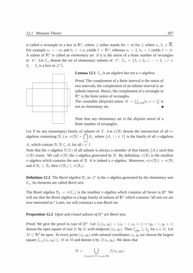
12.1 Measure Theory 307
is called arectangleor a box in Rn, where either stands for< or for ≤ whereai, bi ∈ R.For exampleai = −∞ andbi = +∞ yieldsI = Rn, whereasa1 = 2, b1 = 1 yieldsI = ∅.A subset ofRn is called anelementary setif it is the union of a finite number of rectanglesin Rn. Let En denote the set of elementary subsets ofRn. En = I1 ∪ I2 ∪ · · · ∪ Ir | r ∈N, Ij is a box inRn.
Lemma 12.1 En is an algebra but not aσ-algebra.
Proof. The complement of a finite interval is the union oftwo intervals, the complement of an infinite interval is aninfinite interval. Hence, the complement of a rectangle inRn is the finite union of rectangles.The countable (disjoint) unionM =
⋃n∈N[n, n + 1
2] is
not an elementary set.
Note that any elementary set is thedisjoint union of afinite number of rectangles.
Let B be any (nonempty) family of subsets ofX. Let σ(B) denote the intersection of allσ-algebras containingB, i. e. σ(B) =
⋂
i∈IAi, whereAi | i ∈ I is the family of allσ-algebras
Ai which containB, B ⊆ Ai for all i ∈ I.
Note that theσ-algebraP(X) of all subsets is always a member of that familyAi such thatσ(B) exists. We callσ(B) theσ-algebragenerated byB. By definition,σ(B) is the smallestσ-algebra which contains the sets ofB. It is indeed aσ-algebra. Moreover,σ(σ(B)) = σ(B)
and ifB1 ⊂ B2 thenσ(B1) ⊂ σ(B2).
Definition 12.2 TheBorel algebraBn in Rn is theσ-algebra generated by the elementary setsEn. Its elements are calledBorel sets.
The Borel algebraBn = σ(En) is the smallestσ-algebra which contains all boxes inRn Wewill see that the Borel algebra is a huge family of subsets ofRn which contains “all sets we areever interested in.” Later, we will construct a non-Borel set.
Proposition 12.2 Open and closed subsets ofRn are Borel sets.
Proof. We give the proof in case ofR2. Let Iε(x0, y0) = (x0 − ε, x0 + ε) × (y0 − ε, y0 + ε)
denote the open square of size2ε by 2ε with midpoint(x0, y0). ThenI 1n+1⊆ I 1
nfor n ∈ N. Let
M ⊂ R2 be open. To every point(x0, y0) with rational coordinatesx0, y0 we choose the largestsquareI1/n(x0, y0) ⊆ M in M and denote it byJ(x0, y0). We show that
M =⋃
(x0,y0)∈M,x0,y0∈QJ(x0, y0).

308 12 Measure Theory and Integration
(x,y)
(a,b)0 0
Since the number of rational points inM is at least countable, the rightside is inσ(E2). Now let (a, b) ∈ M arbitrary. SinceM is open, thereexistsn ∈ N such thatI2/n(a, b) ⊆ M . Since the rational pointsare dense inR2, there is rational point(x0, y0) which is contained inI1/n(a, b). Then we have
I 1n(x0, y0) ⊆ I 2
n(a, b) ⊆ M.
Since(a, b) ∈ I 1n(x0, y0) ⊆ J(x0, y0), we have shown thatM is the union of the countable
family of setsJ . Since closed sets are the complements of open sets and complements areagain in theσ-algebra, the assertion follows for closed sets.
Remarks 12.2 (a) We have proved that any open subsetM of Rn is the countable union ofrectanglesI ⊆M .(b) The Borel algebraBn is also theσ-algebra generated by the family of open or closed setsin Rn, Bn = σ(Gn) = σ(Fn). Countable unions and intersections of open or closed sets are inBn.Let us look in more detail at some of the sets inσ(En). Let G andF be the families of all openand closed subsets ofRn, respectively. LetGδ be the collection of all intersection of sequencesof open sets (fromG), and letFσ be the collection of all unions of sequences of sets ofF. Onecan prove thatF ⊂ Gδ andG ⊂ Fσ. These inclusions are strict. Since countable intersectionand unions of countable intersections and union are still countable operations,Gδ,Fσ ⊂ σ(En)
For an arbitrary familyS of sets letSσ be the collection of all unions of sequences of sets inS,and letSδ be the collection of all unions of sequences of sets inS. We can iterate the operationsrepresented byσ andδ, obtaining from the classG the classesGδ, Gδσ, Gδσδ,. . . and fromF theclassesFσ, Fσδ,. . . . It turns out that we have inclusions
G ⊂ Gδ ⊂ Gδσ ⊂ · · · ⊂ σ(En)
F ⊂ Fσ⊂ Fσδ ⊂ · · · ⊂ σ(En).
No two of these classes are equal. There are Borel sets that belong to none of them.
12.1.2 Additive Functions and Measures
Definition 12.3 (a) LetA be an algebra overX. An additive functionor contentµ on A is afunctionµ : A→ [0,+∞] such that
(i) µ(∅) = 0,(ii) µ(A ∪ B) = µ(A) + µ(B) for all A,B ∈ A with A ∩B = ∅.
(b) An additive functionµ is calledcountably additive(or σ-additivein the German literature)onA if for any disjoint familyAn | An ∈ A, n ∈ N, that isAi ∩ Aj = ∅ for all i 6= j, with

12.1 Measure Theory 309
⋃n∈NAn ∈ A we have
µ
(⋃
n∈NAn) =∑
n∈Nµ(An).
(c) A measureis a countably additive function on aσ-algebraA.If X is a set,A a σ-algebra onX andµ a measure onA, then the tripel(X,A, µ) is calleda measure space. Likewise, ifX is a set andA a σ-algebra onX, the pair(X,A) is called ameasurable space.
Notation.We write
∑
n∈NAn in place of⋃
n∈NAn if An is a disjoint family of subsets. The countable
additivity reads as follows
µ(A1 ∪A2 ∪ · · · ) = µ(A1) + µ(A2) + · · · ,
µ
( ∞∑
n=1
An
)=
∞∑
n=1
µ(An).
We sayµ is finite if µ(X) <∞. If µ(X) = 1, we call(X,A, µ) aprobability space. We callµσ-finite if there exist setsAn ∈ A, with µ(An) <∞ andX =
⋃∞n=1An.
Example 12.1 (a) LetX be a set,x0 ∈ X andA = P(X). Then
µ(A) =
1, x0 ∈ A,0, x0 6∈ A
defines a finite measure onA. µ is called thepoint mass concentrated atx0.(b1) LetX be a set andA = P(X). Put
µ(A) =
n, if A hasn elements
+∞, if A has infinitely many elements.
µ is a measure onA, the so calledcounting measure.(b2) LetX be a set andA = P(X). Put
µ(A) =
0, if A has finitely many or countably many elements
+∞, if A has uncountably many elements.
µ is countably additive, notσ-finite.(b3) LetX be a set andA = P(X). Put
µ(A) =
0, if A is finite
+∞, if A is infinite.
µ is additive, notσ-additive.

310 12 Measure Theory and Integration
(c)X = Rn, A = En is the algebra of elementary sets ofRn. EveryA ∈ En is the finite disjointunion of rectanglesA =
∑mk=1 Ik. We setµ(A) =
∑mk=1 µ(Ik) where
µ(I) = (b1 − a1) · · · (bn − an),
if I = (x1, . . . , xn) ∈ Rn | ai xi bi, i = 1, . . . , n andai bi; µ(∅) = 0. Thenµ is anadditive function onEn. It is called theLebesgue contentonRn. Note thatµ is not a measure(sinceA is not aσ-algebra andµ is not yet shown to be countably additive). However, we willsee in Proposition 12.5 below thatµ is evencountably additive. By definition,µ(line inR2) = 0
andµ(plane inR3) = 0.(d) LetX = R, A = E1, andα an increasing function onR. Fora, b inR with a < b set
µα([a, b]) = α(b+ 0)− α(a− 0),
µα([a, b)) = α(b− 0)− α(a− 0),
µα((a, b]) = α(b+ 0)− α(a+ 0),
µα((a, b)) = α(b− 0)− α(a+ 0).
Thenµα is an additive function onE1 if we set
µα(A) =
n∑
i=1
µα(Ii), if A =
n∑
i=1
Ii.
We callµα theLebesgue–Stieltjes content.On the other hand, ifµ : E1 → R is an additive function, thenαµ : R→ R defined by
αµ(x) =
µ((0, x]), x ≥ 0,
−µ((x, 0]), x < 0,
defines an increasing, right-continuous functionαµ onR such thatµ = µαµ . In generalα 6= αµα
since the function on the right hand side is continuous from the right whereasα is, in general,not .
Properties of Additive Functions
Proposition 12.3 LetA be an algebra overX andµ an additive function onA. Then
(a)µ
(n∑
k=1
Ak
)=
n∑
k=1
µ(Ak) if Ak ∈ A, k = 1, . . . , n form a disjoint family ofn
subsets.
(b) µ(A ∪B) + µ(A ∩ B) = µ(A) + µ(B), A,B ∈ A.
(c)A ⊆ B impliesµ(A) ≤ µ(B) (µ is monotone).
(d) If A ⊆ B, A,B ∈ A, and µ(A) < +∞, thenµ(B \A) = µ(B) − µ(A),(µ is subtractive).
12.1 Measure Theory 311
(e)
µ
(n⋃
k=1
Ak
)≤
n∑
k=1
µ(Ak),
if Ak ∈ A, k = 1, . . . , n, (µ is finitely subadditive).
(f) If Ak | k ∈ N is a disjoint family inA and∞∑
k=1
Ak ∈ A. Then
µ
( ∞∑
k=1
Ak
)≥
∞∑
k=1
µ(Ak).
Proof. (a) is by induction. (d), (c), and (b) are easy (cf. Homework34.4).
(e) We can writen⋃
k=1
Ak as the finitedisjointunion ofn sets ofA:
n⋃
k=1
Ak = A1 ∪(A2 \A1
)∪(A3 \ (A1 ∪ A2)
)∪ · · · ∪
(An \ (A1 ∪ · · · ∪An−1)
).
Sinceµ is additive,
µ
(n⋃
k=1
Ak
)=
n∑
k=1
µ (Ak \ (A1 ∪ · · ·Ak−1)) ≤n∑
k=1
µ(Ak),
where we usedµ(B \A) ≤ µ(B) (from (d)).(f) Sinceµ is additive, and monotone
n∑
k=1
µ(Ak) = µ
(n∑
k=1
Ak
)≤ µ
( ∞∑
k=1
Ak
).
Taking the supremum on the left gives the assertion.
Proposition 12.4 Letµ be an additive function on the algebraA. Consider the following state-ments
(a)µ is countably additive.
(b) For any increasing sequenceAn ⊆ An+1, An ∈ A, with∞⋃
n=1
An = A ∈ A we
have limn→∞
µ(An) = µ(A).
(c) For any decreasing sequenceAn ⊇ An+1, An ∈ A, with∞⋂
n=1
An = A ∈ A and
µ(An) <∞ we havelimn→∞
µ(An) = µ(A).
(d) Statement(c) withA = ∅ only.
We have(a) ↔ (b)→ (c)→ (d). In caseµ(X) <∞ (µ is finite), all statements are equivalent.

312 12 Measure Theory and Integration
Proof. (a)→ (b). Without loss of generalityA1 = ∅. PutBn = An \An−1 for n = 2, 3, . . . .ThenBn is a disjoint family withAn = B2 ∪ B3 ∪ · · · ∪ Bn andA =
⋃∞n=1Bn. Hence, by
countable additivity ofµ,
µ(A) =
∞∑
k=2
µ(Bk) = limn→∞
n∑
k=2
µ(Bk) = limn→∞
µ
(n∑
k=2
Bk
)= lim
n→∞µ(An).
(b) → (a). Let An be a family of disjoint sets inA with⋃An = A ∈ A; put Bk =
A1 ∪ · · · ∪Ak. ThenBk is an increasing toA sequence. By (b)
µ(Bn) = µ
(n∑
k=1
Ak
)=
µ is additive
n∑
k=1
µ(Ak) −→n→∞
µ(A) = µ
( ∞∑
k=1
Ak
);
Thus,∞∑
k=1
µ(Ak) = µ
( ∞∑
k=1
Ak
).
(b)→ (c). SinceAn is decreasing toA, A1 \An is increasing toA1 \A. By (b)
µ(A1 \An) −→n→∞
µ(A1 \A),
henceµ(A1)− µ(An) −→n→∞
µ(A1)− µ(A) which implies the assertion.
(c)→ (d) is trivial.Now letµ be finite, in particular,µ(B) <∞ for all B ∈ A. We show (d)→ (b). Let(An) be anincreasing toA sequence of subsetsA,An ∈ A. Then(A \An) is a decreasing to∅ sequence.By (d), µ(A \An) −→
n→∞0. Sinceµ is subtractive (Proposition 12.3 (d)) and all values are finite,
µ(An) −→n→∞
µ(A).
Proposition 12.5 Let α be a right-continuous increasing functionα : R → R, and µα thecorresponding Lebesgue–Stieltjes content onE1. Thenµα is countably additive if.
Proof. For simplicity we writeµ for µα. Recal thatµ((a, b]) = α(b)− α(a). We will performthe proof in case of
(a, b] =
∞⋃
k=1
(ak, bk]
with a disjoint family[ak, bk) of intervals. By Proposition 12.3 (f) we already know
µ ((a, b]) ≥∞∑
k=1
µ((ak, bk]). (12.1)
We prove the opposite direction. Letε > 0. Sinceα is continuous from the right ata, thereexistsa0 ∈ [a, b) such thatα(a0)−α(a) < ε and, similarly, for everyk ∈ N there existsck > bksuch thatα(ck)− α(bk) < ε/2k. Hence,
[a0, b] ⊂∞⋃
k=1
(ak, bk] ⊂∞⋃
k=1
(ak, ck)

12.1 Measure Theory 313
is an open covering of a compact set. By Heine–Borel (Definition 6.14) there exists a finitesubcover
[a0, b] ⊂N⋃
k=1
(ak, ck), hence (a0, b] ⊂N⋃
k=1
(ak, ck],
such that by Proposition 12.3 (e)
µ((a0, b]) ≤N∑
k=1
µ((ak, ck]).
By the choice ofa0 andck,
µ((ak, ck]) = µ((ak, bk]) + α(ck)− α(bk) ≤ µ((ak, bk]) +ε
2k.
Similarly,µ((a, b]) = µ((a, a0]) + µ((a0, b]) such that
µ((a, b]) ≤ µ((a0, b]) + ε ≤N∑
k=1
(µ((ak, bk]) +
ε
2k
)+ ε
≤N∑
k=1
µ((ak, bk]) + 2ε ≤∞∑
k=1
µ((ak, bk]) + 2ε
Sinceε was arbitrary,
µ((a, b]) ≤∞∑
k=1
µ((ak, bk]).
In view of (12.1),µα is countably additive.
Corollary 12.6 The correspondenceµ 7→ αµ from Example 12.1 (d) defines a bijection be-tween countably additive functionsµ onE1 and the monotonically increasing, right-continuousfunctionsα onR (up to constant functions, i. e.α andα+ c define the same additive function).
Historical Note. It was the great achievment ofEmile Borel (1871–1956) that he reallyprovedthe countable additivity of the Lebesgue measure. He realized that the countable additivity ofµis a serious mathematical problem far from being evident.
12.1.3 Extension of Countably Additive Functions
Here we must stop the rigorous treatment of measure theory. Up to now, we know only twotrivial examples of measures (Example 12.1 (a) and (b)). We give an outline of the steps towardthe construction of the Lebesgue measure.
• Construction of anouter measureµ∗ onP(X) from a countably additive functionµ on analgebraA.
• Construction of theσ-algebraAµ of measurable sets.

314 12 Measure Theory and Integration
The extension theory is due to Caratheodory (1914). For a detailed treatment, see [Els02, Sec-tion II.4].
Theorem 12.7 (Extension and Uniqueness)Letµ be a countably additive function on the al-gebraA.(a) There exists an extension ofµ to a measure on theσ-algebraσ(A) which coincides withµon A. We denote the measure onσ(A) also byµ. It is defined as the restriction of the outermeasureµ∗ : P(X)→ [0,∞]
µ∗(A) = inf
∞∑
k=n
µ(An) | A ⊂∞⋃
n=1
An, An ∈ A, n ∈ Nto theµ-measurable setsAµ∗.
(b) This extension is unique, if(X,A, µ) is σ-finite.
(For a proof, see [Bro92, (2.6), p.68])
Remark 12.3 (a) A subsetA ⊂ X is said to beµ-measurableif for all Y ⊂ X
µ∗(Y ) = µ∗(A ∩ Y ) + µ∗(Ac ∩ Y ).
The family ofµ-measurable sets form aσ-algebraAµ∗ .(b) We haveA ⊂ σ(A) ⊂ Aµ∗ andµ∗(A) = µ(A) for all A ∈ A.(c) (X,Aµ∗ , µ
∗) is a measure space, in particular,µ∗ is countably additive on the measurablesetsAµ∗ and we redenote it byµ.
12.1.4 The Lebesgue Measure onRn
Using the facts from the previous subsection we conclude that for any increasing, right contin-uous functionα onR there exists a measureµα on theσ-algebra of Borel sets. We call thismeasure theLebesgue–Stieltjes measure onR. In caseα(x) = x we call it theLebesgue mea-sure. Extending the Lebesgue content on elementary sets ofRn to the Borel algebraBn, weobtain then-dimensional Lebesgue measureλn onRn.
Completeness
A measureµ : A → R+ on aσ-algebraA is said to becompleteif A ∈ A, µ(A) = 0, andB ⊂ A impliesB ∈ A. It turns out that the Lebesgue measureλn on the Borel sets ofRn isnot complete. Adjoining toBn the subsets of measure-zero-sets, we obtain theσ-algebraAλn
of Legesgue measurable setsAλn.
Aλn = σ (Bn ∪ X ⊆ Rn | ∃B ∈ Bn : X ⊂ E, λn(B) = 0) .
The Lebesgue measureλn onAλn is now complete.

12.1 Measure Theory 315
Remarks 12.4 (a) The Lebesgue measure is invariant under themotion groupof Rn. Moreprecisely, letO(n) = T ∈ Rn×n | T⊤T = T T⊤ = En be the group of real orthogonaln× n-matrices (“motions”), then
λn(T (A)) = λn(A), A ∈ Aλn , T ∈ O(n).
(b)λn is translation invariant, i. e.λn(A) = λn(x+A) for all x ∈ Rn. Moreover, the invarianceof λn under translations uniquely characterizes the Lebesgue measureλn: If λ is a translationinvariant measure onBn, thenλ = cλn for somec ∈ R+.(c) There exist non-measurable subsets inRn. We construct a subsetE ofR that is not Lebesguemeasurable.We writex ∼ y if x − y is rational. This is an equivalence relation sincex ∼ x for all x ∈ R,x ∼ y impliesy ∼ x for all x andy, andx ∼ y andy ∼ z impliesx ∼ z. LetE be a subset of(0, 1) that contains exactly one point in every equivalence class.(the assertion that there is sucha setE is a direct application of theaxiom of choice). We claim thatE is not measurable. LetE + r = x+ r | x ∈ E. We need the following two properties ofE:
(a) If x ∈ (0, 1), thenx ∈ E + r for some rationalr ∈ (−1, 1).(b) If r ands are distinct rationals, then(E + r) ∩ (E + s) = ∅.
To prove (a), note that for everyx ∈ (0, 1) there existsy ∈ E with x ∼ y. If r = x − y, thenx = y + r ∈ E + r.To prove (b), suppose thatx ∈ (E + r) ∩ (E + s). Thenx = y + r = z + s for somey, z ∈ E.Sincey−z = s− r 6= 0, we havey ∼ z, andE contains two equivalent points, in contradictionto our choice ofE.Now assume thatE is Lebesgue measurable withλ(E) = α. DefineS =
⋃(E + r) where
the union is over all rationalr ∈ (−1, 1). By (b), the setsE + r are pairwise disjoint; sinceλis translation invariant,λ(E + r) = λ(E) = α for all r. SinceS ⊂ (−1, 2), λ(S) ≤ 3. Thecountable additivity ofλ now forcesα = 0 and henceλ(S) = 0. But (a) implies(0, 1) ⊂ S,hence1 ≤ λ(S), and we have a contradiction.(d) Any countable set has Lebesgue measure zero. Indeed, every single point is a box withedges of length0; henceλ(pt) = 0. Sinceλ is countably additive,
λ(x1, x2, . . . , xn, . . . ) =
∞∑
n=1
λ(xn) = 0.
In particular, the rational numbers have Lebesgue measure0, λ(Q) = 0.(e) There are uncountable sets with measure zero. The Cantorset (Cantor: 1845–1918, inventorof set theory) is a prominent example:
C =
∞∑
i=1
ai3i
∣∣∣∣∣ ai ∈ 0, 2 ∀ i ∈ N ;
Obviously,C ⊂ [0, 1]; C is compact and can be written as the intersection of a decreasingsequence(Cn) of closed subsets;C1 = [0, 1/3] ∪ [2/3, 1], λ(C1) = 2/3, and, recursively,
Cn+1 =1
3Cn ∪
(2
3+
1
3Cn
)=⇒ λ(Cn+1) =
1
3λ(Cn) +
1
3λ
(Cn +
2
3
)=
2
3λ(Cn).

316 12 Measure Theory and Integration
It turns out thatCn =∑∞
i=1ai
3i
∣∣ iai ∈ 0, 2 ∀ i = 1, . . . , n
Clearly,
λ(Cn+1) =2
3λ(Cn) = · · · =
(2
3
)nλ(C1) =
(2
3
)n+1
.
By Proposition 12.4 (c),λ(C) = limn→∞
λ(Cn) = 0. However,C has the same cardinality as
0, 2N ∼= 0, 1N ∼= R which is uncountable.
12.2 Measurable Functions
Let A be aσ-algebra overX.
Definition 12.4 A real functionf : X → R is calledA-measurableif for all a ∈ R the setx ∈ X | f(x) > a belongs toA.A complex functionf : X → C is said to beA-measurableif both Re f and Im f areA-measurable.A function f : U → R, U ⊂ Rn, is said to be aBorel functionif f is Bn-measurable, i. e.f ismeasurable with respect to the Borel algebra onRn.A function f : U → V , U ⊂ Rn, V ⊂ Rm, is called aBorel functionif f−1(B) is a Borel setfor all Borel setsB ⊂ V . It is part of homework 39.3 (b) to prove that in casem = 1 thesedefinitions coincide. Also,f = (f1, . . . , fm) is a Borel function if allfi are.
Note thatx ∈ X | f(x) > a = f−1((a,+∞)). From Proposition 12.8 below it becomes clearthat the last two notions are consistent. Note that no measure on(X,A) needs to be specifiedto define a measurable function.
Example 12.2 (a) Any continuous functionf : U → R, U ⊂ Rn, is a Borel function. Indeed,sincef is continuous and(a,+∞) is open,f−1((a,+∞)) is open as well and hence a Borel set(cf. Proposition 12.2).(b) The characteristic functionχA is A-measurable if and only ifA ∈ A (see homework 35.3).(c) Letf : U → V andg : V →W be Borel functions. Thengf : U → W is a Borel function,too. Indeed, for any Borel setC ⊂ W , g−1(C) is a Borel set inV sinceg is a Borel function.Sincef is a Borel function(gf)−1(C) = f−1(g−1(C)) is a Borel subset ofU which shows theassertion.
Proposition 12.8 Letf : X → R be a function. The following are equivalent
(a)x | f(x) > a ∈ A for all a ∈ R (i. e. f is A-measurable).(b) x | f(x) ≥ a ∈ A for all a ∈ R.(c) x | f(x) < a ∈ A for all a ∈ R.(d) x | f(x) ≤ a ∈ A for all a ∈ R.(e)f−1(B) ∈ A for all Borel setsB ∈ B1.
Proof. (a)→ (b) follows from the identity
[a,+∞] =⋂
n∈N (a− 1/n,+∞]

12.2 Measurable Functions 317
and the invariance of intersections under preimages,f−1(A ∩ B) = f−1(A) ∩ f−1(B).Sincef is A-measurable andA is aσ-algebra, the countable intersection on the right is inA.(a)→ (d) follows fromx | f(x) ≤ a = x | f(x) > ac. The remaining directions are leftto the reader (see also homework 35.5).
Remark 12.5 (a) Let f, g : X → R be A-measurable. Thenx | f(x) > g(x) andx |f(x) = g(x) are inA. Proof. Since
x | f(x) < g(x) =⋃
q∈Q (x | f(x) < q ∩ x | q < g(x)) ,
and all setsf < q andq < g the right are inA, and on the right there is a countable union,the right hand side is inA. A similar argument works forf > g. Note that the setsf ≥ gandf ≤ g are the complements off < g andf > g, respectively; hence they belong toA as well. Finally,f = g = f ≥ g ∩ f ≤ g.
(b) It is not difficult to see that for any sequence(an) of real numbers
limn→∞
an = infn∈N sup
k≥nak and lim
n→∞an = sup
n∈N infk≥n
ak. (12.2)
As a consequence we can construct new mesurable functions using sup andlimn→∞. Let (fn)be a sequence ofA-measurable real functions onX. Thensup
n∈N fn, infn∈N fn, lim
n→∞fn, lim
n→∞fn are
A-measurable. In particularlimn→∞
fn is measurable if the limit exists.
Proof. Note that for alla ∈ R we have
sup fn ≤ a =⋂
n∈Nfn ≤ a.
Since allfn are measurable, so issup fn. A similar proof works forinf fn. By (12.2), limn→∞
fn
and limn→∞
fn, are measurable, too.
Proposition 12.9 Letf, g : X → R Borel functions onX ⊂ Rn. Thenαf + βg, f · g, and| f |are Borel functions, too.
Proof. The functionh(x) = (f(x), g(x)) : X → R2 is a Borel function since its coordinatefunctions are so. Since the sums(x, y) = x + y and the productp(x, y) = xy are continuousfunctions, the compositionssh andph are Borel functions by Example 12.2 (c). Since theconstant functionsα andβ are Borel, so areαf , βg, and finallyαf + βg. Hence, the Borelfunctions overX form a linear space, moreover a real algebra. In particular−f is Borel and sois | f | = maxf,−f.
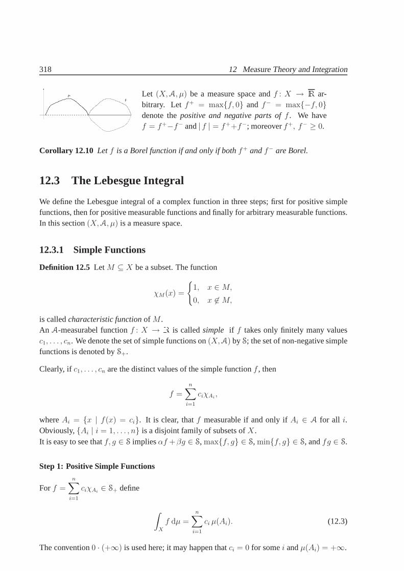
318 12 Measure Theory and Integration
f+
f-
Let (X,A, µ) be a measure space andf : X → R ar-bitrary. Let f+ = maxf, 0 and f− = max−f, 0denote thepositive and negative parts off . We havef = f+−f− and| f | = f++f−; moreoverf+, f− ≥ 0.
Corollary 12.10 Letf is a Borel function if and only if bothf+ andf− are Borel.
12.3 The Lebesgue Integral
We define the Lebesgue integral of a complex function in threesteps; first for positive simplefunctions, then for positive measurable functions and finally for arbitrary measurable functions.In this section(X,A, µ) is a measure space.
12.3.1 Simple Functions
Definition 12.5 LetM ⊆ X be a subset. The function
χM(x) =
1, x ∈M,
0, x 6∈M,
is calledcharacteristic functionof M .An A-measurabel functionf : X → R is calledsimple if f takes only finitely many valuesc1, . . . , cn. We denote the set of simple functions on(X,A) by S; the set of non-negative simplefunctions is denoted byS+.
Clearly, if c1, . . . , cn are the distinct values of the simple functionf , then
f =
n∑
i=1
ciχAi,
whereAi = x | f(x) = ci. It is clear, thatf measurable if and only ifAi ∈ A for all i.Obviously,Ai | i = 1, . . . , n is a disjoint family of subsets ofX.It is easy to see thatf, g ∈ S impliesαf +βg ∈ S, maxf, g ∈ S, minf, g ∈ S, andfg ∈ S.
Step 1: Positive Simple Functions
Forf =
n∑
i=1
ciχAi∈ S+ define
∫
X
f dµ =
n∑
i=1
ci µ(Ai). (12.3)
The convention0 · (+∞) is used here; it may happen thatci = 0 for somei andµ(Ai) = +∞.

12.3 The Lebesgue Integral 319
Remarks 12.6 (a) Sinceci ≥ 0 for all i, the right hand side is well-defined inR.
(b) Given another presentation off , say,f(x) =
m∑
j=1
djχBj,m∑
j=1
dj µ(Bj) gives the same value
as (12.3).
The following properties are easily checked.
Lemma 12.11 For f, g ∈ S+, A ∈ A, c ∈ R+ we have
(1)∫XχA dµ = µ(A).
(2)∫Xcf dµ = c
∫Xf dµ.
(3)∫X
(f + g) dµ =∫Xf dµ+
∫Xg dµ.
(4) f ≤ g implies∫Xf dµ ≤
∫Xg dµ.
12.3.2 Positive Measurable Functions
The idea is to approximate a positive measurable function with an increasing sequence of posi-tive simple ones.
Theorem 12.12Let f : X → [0,+∞] be measurable. There exist simple functionssn, n ∈ N,onX such that
(a) 0 ≤ s1 ≤ s2 ≤ · · · ≤ f .
(b) sn(x) −→n→∞
f(x), asn→∞, for everyx ∈ X.
E12 11
3/4
ba
f
E24
E24
F
1
1/2
0
y
x1
E E12 E
11
s1
Example.X = (a, b), n = 1,1 ≤ i ≤ 2. Then
E11 = f−1
([0,
1
2
)),
E12 = f−1
((1
2, 1
)),
F2 = f−1 ([1,+∞]) .
Proof. Forn ∈ N and for1 ≤ i ≤ n2n, define
Eni = f−1
([i− 1
2n,i
2n
))and Fn = f−1([n,∞])
and put
sn =n2n∑
i=1
i− 1
2nχEni
+ nχFn .

320 12 Measure Theory and Integration
Proposition 12.8 shows thatEni andFn are measurable sets. It is easily seen that the functionssn satisfy (a). Ifx is such thatf(x) < +∞, then
0 ≤ f(x)− sn(x) ≤1
2n(12.4)
as soon asn is large enough, that is,x ∈ Eni for somen, i ∈ N and notx ∈ Fn. If f(x) = +∞,thensn(x) = n; this proves (b).
From (12.4) it follows, thatsn f uniformly onX if f is bounded.
Step 2: Positive Measurable Real Functions
Definition 12.6 (Lebesgue Integral)Let f : X → [0,+∞] be measurable. Let(sn) be anincreasing sequence of non-negative simple functionssn converging tof(x) for all x ∈ X,limn→∞
sn(x) = supn∈N sn(x) = f(x). Define
∫
X
f dµ = limn→∞
∫
X
sn dµ = supn∈N∫X sn dµ (12.5)
and call this number in[0,+∞] theLebesgue integral off(x) overX with respect to the mea-sureµ or µ-integral off overX.
The definition of the Lebesgue integral does not depend on thespecial choice of the increasingfunctionssn ր f . One can define
∫
X
f dµ = sup
∫
X
s dµ | s ≤ f, ands is a simple function
.
Observe, that we apparently have two definitions for∫Xf dµ if f is a simple function. However
these assign the same value to the integral sincef is the largest simple function greater than orequal tof .
Proposition 12.13 The properties(1) to (4) from Lemma 12.11 hold for any non-negative mea-surable functionsf, g : X → [0,+∞], c ∈ R+.
(Without proof.)
Step 3: Measurable Real Functions
Let f : X → R be measurable andf+(x) = max(f, 0), f−(x) = max(−f(x), 0). Thenf+
andf− are both positive and measurable. Define∫
X
fdµ =
∫
X
f+dµ−∫
X
f−dµ
if at least one of the integrals on the right is finite. We say that f is µ-integrableif both arefinite.

12.3 The Lebesgue Integral 321
Step 4: Measurable Complex Functions
Definition 12.7 (Lebesgue Integral—Continued)A complex, measurable functionf : X → C is calledµ-integrableif
∫
X
| f | dµ <∞.
If f = u + iv is µ-integrable, whereu = Re f andv = Im f are the real and imaginary partsof f , u andv are real measurable functions onX. Define theµ-integral off overX by
∫
X
f dµ =
∫
X
u+ dµ−∫
X
u− dµ+ i
∫
X
v+ dµ− i
∫
X
v− dµ. (12.6)
These four functionsu+, u−, v+, andv− are measurable, real, and non-negative. Since we haveu+ ≤ |u | ≤ | f | etc., each of these four integrals is finite. Thus, (12.6) defines the integral onthe left as a complex number.
We defineL 1(X,µ) to be the collection of all complexµ-integrable functionsf onX.Note that for an integrable functionsf ,
∫Xf dµ is a finite number.
Proposition 12.14 Letf, g : X → C be measurable.
(a) f is µ-integrable if and only if| f | is µ-integrable and we have∣∣∣∣∫
X
f dµ
∣∣∣∣ ≤∫
X
| f | dµ.
(b) f is µ-integrable if and only if there exists an integrable functionh with | f | ≤h.
(c) If f, g are integrable, so isc1f + c2g where∫
X
(c1f + c2g) dµ = c1
∫
X
f dµ+ c2
∫
X
g dµ.
(d) If f ≤ g onX, then∫Xf dµ ≤
∫Xg dµ.
It follows that the setL 1(X,µ) of µ-integrable complex-valued functions onX is a linearspace. The Lebesgue integral defines a positive linear functional onL 1(X,µ). Note that (b)implies that any measurable and bounded functionf on a spaceX with µ(X) <∞ is integrable.
Step 5:∫
Af dµ
Definition 12.8 Let A ∈ A, f : X → R or f : X → C measurable. The functionf is calledµ-integrable overA if χA f is µ-integrable overX. In this case we put,
∫
A
f dµ =
∫
X
χA f dµ.
In particular, Lemma 12.11 (1) now reads∫A
dµ = µ(A).

322 12 Measure Theory and Integration
12.4 Some Theorems on Lebesgue Integrals
12.4.1 The Role Played by Measure Zero Sets
Equivalence Relations
LetX be a set andR ⊂ X ×X. Fora, b ∈ X we writea ∼ b if (a, b) ∈ R.
Definition 12.9 (a) The subsetR ⊂ X×X is said to be anequivalence relationif R is reflexive,symmetricandtransitive, that is,
(r) ∀x ∈ X : x ∼ x.
(s) ∀x, y ∈ X : x ∼ y =⇒ y ∼ x.(t) ∀x, y, z ∈ X : x ∼ y ∧ y ∼ z =⇒ x ∼ z.
Fora ∈ X the seta := x ∈ X | x ∼ a is called theequivalence classof a. We havea = b ifand only ifa ∼ b.(b) A partition P of X is a disjoint familyP = Aα | α ∈ I of subsetsAα ⊂ X such that∑α∈I
Aα = X.
The set of equivalence classes is sometimes denoted byX/ ∼.
Example 12.3 (a) OnZ definea ∼ b if 2 | (a−b). a andb are equivalent if both are odd or bothare even. There are two equivalence classes,1 = −5 = 2Z + 1 (odd numbers),0 = 100 = 2Zeven numbers.(b) LetW ⊂ V be a subspace of the linear spaceV . Forx, y ∈ V definex ∼ y if x − y ∈ W .This is an equivalence relation, indeed, the relation is reflexive sincex − x = 0 ∈ W , itis symmetric sincex − y ∈ W implies y − x = −(x − y) ∈ W , and it is transitive sincex− y, y− z ∈W implies that there sum(x− y) + (y− z) = x− z ∈W such thatx ∼ z. Onehas0 = W andx = x+W := x+w | w ∈W. Set set of equivalence classes with respect tothis equivalence relation is called thefactor spaceor quotient spaceof V with respect toW andis denoted byV/W . The factor space becomes a linear space if we definex + y := x+ y andλ x = λx, λ ∈ C. Addition is indeed well-defined sincex ∼ x′ andy ∼ y′, say,x− x′ = w1,y− y′ = w2, w1, w2 ∈W impliesx+ y− (x′ + y′) = w1 +w2 ∈W such thatx+ y = x′ + y′.(c) Similarly as in (a), form ∈ N define the equivalence relationa ≡ b (modm) if m | (a− b).We say “a is congruentb modulom”. This defines a partition of the integers intom disjointequivalence classes0, 1, . . . , m− 1, wherer = am+ r | a ∈ Z.(d) Two triangles in the plane are equivalent if
(1) there exists atranslationsuch that the first one is mapped onto the second one.(2) there exists arotationaround(0, 0)
(3) there exists amotion(rotation or translation or reflexion or composition)
Then (1) – (3) define different equivalence relations on triangles or more generally on subsetsof the plane.(e) Cardinality of sets is an equivalence relation.

12.4 Some Theorems on Lebesgue Integrals 323
Proposition 12.15 (a) Let∼ be an equivalence relation onX. ThenP = x | x ∈ X definesa partition onX denoted byP∼.(b) Let P be a partition onX. Thenx ∼ y if there existsA ∈ P with x, y ∈ A defines anequivalence relation∼P onX.(c)∼P∼=∼ andP∼P
= P.
LetP be a property which a pointx may or may not have. For instance,P may be the property“f(x) > 0” if f is a given function or “(fn(x)) converges” if(fn) is a given sequence offunctions.
Definition 12.10 If (X,A, µ) is a measure space andA ∈ A, we say“ P holds almost every-where on A”, abbreviated by “P holds a. e. onA”, if there existsN ∈ A such thatµ(N) = 0
andP holds for every pointx ∈ A \N .
This concept of course strongly depends on the measureµ, and sometimes we write a. e. toemphasize the dependence onµ.(a) Main example. On the set of measurable functions onX, f : X → C we define an equiva-lence relation by
f ∼ g, if f = g a. e. onX.
This is indeed an equivalence relation sincef(x) = f(x) for all x ∈ X, f(x) = g(x) impliesg(x) = f(x). Let f = g a. e. onX andg = h a. e. onX, that is, there existM,N ∈ A withµ(M) = µ(N) = 0 andf(x) = g(x) for all x ∈ X \M , g(x) = h(x) for all x ∈ N . Hence,f(x) = h(x) for all x ∈ M ∪ N . Since0 ≤ µ(M ∪ N) ≤ µ(M) + µ(N) = 0 + 0 = 0 byProposition 12.3 (e),µ(M ∪N) = 0 and finallyf = h a. e. onX.(b) Note thatf = g a. e. onX implies
∫
X
f dµ =
∫
X
g dµ.
Indeed, letN denote the zero-set wheref 6= g. Then∣∣∣∣∫
X
f dµ−∫
X
g dµ
∣∣∣∣ ≤∫
X
| f − g | dµ =
∫
N
| f − g | dµ+
∫
X \N| f − g | dµ
≤ µ(N)(∞) + µ(X \N) · 0 = 0.
Here we used that for disjoint setsA,B ∈ A,∫
A∪Bf dµ =
∫
X
χA∪Bf dµ =
∫
X
χAf dµ+
∫
X
χBf dµ =
∫
A
f dµ+
∫
B
f dµ.
Proposition 12.16 Letf : X → [0,+∞] be measurable. Then∫Xf dµ = 0 if and only iff = 0 a. e. onX.
Proof. By the above argument in (b),f = 0 a. e. implies∫Xf dµ =
∫X
0 dµ = 0 which provesone direction. The other direction is homework 40.4.

324 12 Measure Theory and Integration
12.4.2 The spaceLp(X, µ)
For any measurable functionf : X → C and any realp, 1 ≤ p <∞ define
‖f‖p =
(∫
X
| f |p dµ
) 1p
. (12.7)
This number may be finite or∞. In the first case,| f |p is integrable and we writef ∈ L1(X,µ).
Proposition 12.17 Letp, q ≥ 1 be given such that1p
+ 1q
= 1.(a) Letf, g : X → C be measurable functions such thatf ∈ L p andg ∈ L q.Thenfg ∈ L 1 and
∫
X
| fg | dµ ≤ ‖f‖p ‖g‖q (Holder inequality). (12.8)
(b) Letf, g ∈ L q. Thenf + g ∈ L q and
‖f + g‖q ≤ ‖f‖q + ‖g‖q , (Minkowski inequality). (12.9)
Idea of proof. Holder follows from Young’s inequality (Proposition 1.31, as in the calssical caseof Holder’s inequality inRn, see Proposition 1.32Minkowski’s inequality follows from Holder’s inequalityas in Propostion 1.34Note that Minkowski implies thatf, g ∈ L p yields‖f + g‖ < ∞ such thatf + g ∈ L p. Inparticular,L p is a linaer space.Let us check the properties of‖·‖p. For all measurablef, g we have
‖f‖p ≥ 0,
‖λf‖p = |λ | ‖f‖p ,‖f + g‖ ≤ ‖f‖+ ‖g‖ .
All properties of a norm, see Definition 6.9 at page 179 are satisfied except for the definitness:‖f‖p = 0 imlies
∫X| f |p dµ = 0 implies by Proposition 12.16,| f |p = 0 a. e. impliesf = 0
a. e. . However, it does not implyf = 0. To overcome this problem, we use the equivalecerelationf = g a. e. and consider from now on onlyequivalence classesof functions inL
p, thatis we identify functionsf andg which are equal a. e. .The spaceN = f : X → C | f is measurable andf = 0 a. e. is a linear subspace ofL p(X,µ) for all all p, andf = g a. e. if and only iff − g ∈ N. Then the factor spaceL p/N,see Example 12.3 (b) is again a linear space.
Definition 12.11 Let (X,A, µ) be a measure space.Lp(X,µ) denotes the set of equivalenceclasses of functions ofL p(X,µ) with respect to the equivalence relationf = g a. e. that is,
Lp(X,µ) = Lp(X,µ)/N
is the quotient space.(Lp(X,µ), ‖·‖p) is a normed space. With this normLp(X,µ) is complete.

12.4 Some Theorems on Lebesgue Integrals 325
Example 12.4 (a) We haveχQ = 0 in Lp(R, λ) sinceχQ = 0 a. e. onR with respect to theLebesgue measure (note thatQ is a set of measure zero).(b) In case of sequence spacesL p(N) with respect to the counting measure,L p = Lp sincef = 0 a. e. impliesf = 0.(c) f(x) = 1
xα , α > 0 is in L2(0, 1) if and only if 2α < 1. We identify functions and theirequivalence classes.
12.4.3 The Monotone Convergence Theorem
The following theorem about the monotone convergence by Beppo Levi (1875–1961) is one ofthe most important in the theory of integration. The theoremholds for anarbitrary increasingsequence of measurable functions with, possibly,
∫Xfn dµ = +∞.
Theorem 12.18 (Monotone Convergence Theorem/Lebesgue)Let (fn) be a sequence ofmeasurable functions onX and suppose that
(1) 0 ≤ f1(x) ≤ f2(x) ≤ · · · ≤ +∞ for all x ∈ X,(2) fn(x) −→
n→∞f(x), for everyx ∈ X.
Thenf is measurable, and
limn→∞
∫
X
fn dµ =
∫
X
f dµ =
∫
X
(limn→∞
fn
)dµ.
(Without proof) Note, thatf is measurable is a consequence of Remark 12.5 (b).
Corollary 12.19 (Beppo Levi) Let fn : X → [0,+∞] be measurable for alln ∈ N, and
f(x) =∞∑
n=1
fn(x) for x ∈ X. Then
∫
X
∞∑
n=1
fn dµ =∞∑
n=1
∫
X
fn dµ.
Example 12.5 (a) LetX = N, A = P(N) the σ-algebra of all subsets, andµ the countingmeasure onN. The functions onN can be identified with the sequences(xn), f(n) = xn.Trivially, any function isA-measurable.What is
∫N xn dµ? First, letf ≥ 0. For a simple functiongn, given bygn = xnχn, we obtain∫gn dµ = xnµ(n) = xn. Note thatf =
∞∑
n=1
gn andgn ≥ 0 sincexn ≥ 0. By Corollary 12.19,
∫N f dµ =
∞∑
n=1
∫N gn dµ =
∞∑
n=1
xn.
Now, let f be arbitrary integrable, i. e.∫N | f | dµ < ∞; thus
∑∞n=1 |xn | < ∞. Therefore,
(xn) ∈ L 1(N, µ) if and only if∑xn convergesabsolutely. The space of absolutely convergent
series is denoted byℓ1 or ℓ1(N).

326 12 Measure Theory and Integration
(b) Letanm ≥ 0 for all n,m ∈ N. Then
∞∑
n=1
∞∑
m=1
amn =
∞∑
m=1
∞∑
n=1
amn.
Proof. Consider the measure space(N,P(N), µ) from (a). Forn ∈ N define functionsfn(m) =
amn. By Corollary 12.19 we then have
∫
X
∞∑
n=1
fn(m)
︸ ︷︷ ︸f(m)
dµ =
∫
X
f dµ =(a)
∞∑
m=1
f(m) =∞∑
m=1
∞∑
n=1
amn
=
∞∑
n=1
∫
X
fn(m) dµ =
∞∑
n=1
∞∑
m=1
amn.
Proposition 12.20 Letf : X → [0,+∞] be measurable. Then
ϕ(A) =
∫
A
f dµ, A ∈ A
defines a measureϕ onA.
Proof. Sincef ≥ 0, ϕ(A) ≥ 0 for all A ∈ A. Let (An) be a countable disjoint family ofmeasurable setsAn ∈ A and letA =
∑∞n=1An. By homework 40.1,χA =
∑∞n=1 χAn and
therefore
ϕ(A) =
∫
A
f dµ =
∫
X
χAf dµ =
∫
X
∞∑
n=1
χAnf dµ =B.Levi
∞∑
n=1
∫
X
χAnf dµ
=
∞∑
n=1
∫
An
f dµ =
∞∑
n=1
ϕ(An).
12.4.4 The Dominated Convergence Theorem
Besides the monotone convergence theorem the present theorem is the most important one. It isdue to Henry Lebesgue. The great advantage, compared with Theorem6.6, is thatµ(X) =∞ isallowed, that is, non-compact domainsX are included. We only need thepointwiseconvergenceof (fn), not theuniformconvergence. The main assumtion here is the existence of an integrableupper bound for allfn.
Theorem 12.21 (Dominated Convergence Theorem of Lebesgue)Let fn : X → R org, fn : X → C be measurable functions such that

12.4 Some Theorems on Lebesgue Integrals 327
(1) fn(x)→ f(x) asn→∞ a. e. onX,
(2) | fn(x) | ≤ g(x) a. e. onX,
(3)∫
X
g dµ < +∞.
Thenf is measurable and integrable,∫X| f | dµ <∞, and
limn→∞
∫
X
fn dµ =
∫
X
f dµ =
∫
X
limn→∞
fn dµ,
limn→∞
∫
X
| fn − f | dµ = 0. (12.10)
Note, that (12.10) shows that(fn) converges tof in the normed spaceL1(X,µ).
Example 12.6 (a) LetAn ∈ A, n ∈ N, A1 ⊂ A2 ⊂ · · · be an increasing sequence with⋃
n∈NAn = A. If f ∈ L 1(A, µ), thenf ∈ L 1(An) for all n and
limn→∞
∫
An
f dµ =
∫
A
f dµ. (12.11)
Indeed, the sequence(χAn f) is pointwise converging toχAf sinceχA(x) = 1 iff x ∈ A
iff x ∈ An for all n ≥ n0 iff limn→∞ χAn(x) = 1. Moreover,|χAnf | ≤ |χAf | which isintegrable. By Lebesgue’s theorem,
limn→∞
∫
An
f dµ = limn→∞
∫
X
χAnf =
∫
X
χAf dµ =
∫
A
f dµ.
However, if we do not assumef ∈ L1(A, µ), the statement is not true (see Remark 12.7 be-
low).Exhausting theorem.Let (An) be an increasing sequencce of measurable sets andA =⋃∞n=1An. suppose thatf is measurable, and
∫Anf dµ is a bounded sequence. Thenf ∈
L 1(A, µ) and (12.11) holds.(b) Let fn(x) = (−1)nxn on [0, 1]. The sequence is dominated by the integrable function1 ≥ | fn(x) | for all x ∈ [0, 1]. Hencelimn→∞
∫[0,1]
fndλ = 0 =∫[0,1]
limn→∞ fndλ.
12.4.5 Application of Lebesgue’s Theorem to Parametric Integrals
As a direct application of the dominated convergence theorem we now treat parameter depen-dent integrals see Propostions 7.22 and 7.23
Proposition 12.22 (Continuity) Let U ⊂ Rn be an open connected set,t0 ∈ U , andf : Rm × U → R be a function. Assume that
(a) for a.e.x ∈ Rm, the functiont 7→ f(x, t) is continuous att0,(b) There exists an integrable functionF : Rm → R such that for everyt ∈ U ,
| f(x, t) | ≤ F (x) a.e. onRm.

328 12 Measure Theory and Integration
Then the function
g(t) =
∫Rm
f(x, t) dx
is continuous att0.
Proof. First we note that for any fixedt ∈ U , the functionft(x) = f(x, t) is integrable onRm since it is dominated by the integrable functionF . We have to show that for any sequencetj → t0, tj ∈ U , g(tj) tends tog(t0) asn→ ∞. We setfj(x) = f(x, tj) andf0(x) = f(x, t0)
for all n ∈ N. By (b) we have
f0(x) = limj→∞
fj(x), a. e.x ∈ Rm.
By (a) and (c), the assumptions of the dominated convergencetheorem are satisfied and thus
limj→∞
g(tj) = limj→∞
∫Rm
fj(x) dx =
∫Rm
limj→∞
fj(x) dx =
∫Rm
f0(x) dx = g(t0).
Proposition 12.23 (Differentiation under the Integral Sign) Let I ⊂ R be an open intervalandf : Rm × I → R be a function such that
(a) for everyt ∈ I the functionx 7→ f(x, t) is integrable,(b) for almost allx ∈ Rm, the functiont 7→ f(x, t) is finite and continuouslydifferentiable,(c) There exists an integrable functionF : Rm → R such that for everyt ∈ I∣∣∣∣
∂f
∂t(x, t)
∣∣∣∣ ≤ F (x), a.e.x ∈ Rm.
Then the functiong(t) =∫Rm f(x, t) dx is differentiable onI with
g′(t) =
∫Rm
∂f
∂t(x, t) dx.
The proof uses the previous theorem about the continuity of the parametric integral. A detailedproof is to be found in [Kon90, p. 283].
Example 12.7 (a) Let f ∈ L1(R). Then the Fourier transformf : R→ C,
f(t) = 1√2π
∫R e−itx f(x) dx is continuous onR, see homework 41.3.
(b) LetK ⊂ R3 be a compact subset andρ : K → R integrable, the Newton potential (withmass densityρ) is given by
u(t) =
∫
K
ρ(x)
‖x− t‖ dx, t 6∈ K.
Thenu(t) is a harmonic function onR3 \K.Similarly, if K ⊂ R2 is compact andρ ∈ L (K), the Newton potential is given by
u(t) =
∫
K
ρ(x) log ‖x− t‖ dx, t 6∈ K.
Thenu(t) is a harmonic function onR2 \K.

12.4 Some Theorems on Lebesgue Integrals 329
12.4.6 The Riemann and the Lebesgue Integrals
Proposition 12.24 Letf be a bounded function on the finite interval[a, b].(a)f is Riemann integrable on[a, b] if and only iff is continuous a. e. on[a, b].(b) If f is Riemann integrable on[a, b], thenf is Lebesgue integrable, too. Both integralscoincide.Let I ⊂ R be an interval such thatf is Riemann integrable on all compact subintervals ofI.(c) f is Lebesgue integrable onI if and only if | f | is improperly Riemann integrable onI (seeSection 5.4); both integrals coincide.
Remarks 12.7 (a) The characteristic functionχQ on [0, 1] is Lebesgue but not Riemann inte-grable;χQ is nowhere continuous on[0, 1].(b) The (improper) Riemann integral
∫ ∞
1
sin x
xdx
converges (see Example 5.11); however, the Lebesgue integral does not exist since the integraldoes not converge absolutely. Indeed, for non-negative integersn ≥ 1 we have with somec > 0
∫ (n+1)π
nπ
∣∣∣∣sin x
x
∣∣∣∣ dx ≥ 1
(n+ 1)π
∫ (n+1)π
nπ
| sin x | dx =c
(n + 1)π;
hence ∫ (n+1)π
π
∣∣∣∣sin x
x
∣∣∣∣ dx ≥ c
π
n∑
k=1
1
k + 1.
Since the harmonic series diverges, so does the integral∫∞1
∣∣ sinxx
∣∣ dx.
12.4.7 Appendix: Fubini’s Theorem
Theorem 12.25Let(X1,A1, µ1) and(X2,A2, µ2) beσ-finite measure spaces, letf be anA1⊗A2-measurable function andX = X1 ×X2.(a) If f : X → [0,+∞], ϕ(x1) =
∫X2
f(x1, x2) dµ2, ψ(x2) =∫X1
f(x1, x2) dµ1, then
∫
X2
ψ(x2) dµ2 =
∫
X1×X2
f d(µ1 ⊗ µ2) =
∫
X1
ϕ(x1) dµ1.
(b) If f ∈ L 1(X,µ1 ⊗ µ2) then∫
X1×X2
f d(µ1 ⊗ µ2) =
∫
X2
(∫
X1
f(x1, x2) dµ1
)dµ2.
HereA1 ⊗ A2 denotes the smallestσ-algebra overX, which contains all setsA × B, A ∈ A1
andB ∈ A2. Defineµ(A×B) = µ1(A)µ2(B) and extendµ to a measureµ1⊗µ2 onA1⊗A2.
Remark 12.8 In (a), as in Levi’s theorem, we don’t need any assumption onf to change theorder of integration sincef ≥ 0. In (b) f is an arbitrary measurable function onX1 × X2,however, the integral
∫X| f | dµ needs to be finite.

330 12 Measure Theory and Integration

Chapter 13
Hilbert Space
Functional analysis is a fruitful interplay between linearalgebra and analysis. One definesfunction spaces with certain properties and certain topologies and considers linear operatorsbetween such spaces. The friendliest example of such spacesare Hilbert spaces.This chapter is divided into two parts—one describes the geometry of a Hilbert space, thesecond is concerned with linear operators on the Hilbert space.
13.1 The Geometry of the Hilbert Space
13.1.1 Unitary Spaces
LetE be a linear space overK = R or overK = C.
Definition 13.1 An inner productonE is a function〈· , ·〉 : E ×E → K with
(a) 〈λ1x1 + λ2x2 , y〉 = λ1 〈x1 , y〉+ λ2 〈x2 , y〉 (Linearity)(b) 〈x , y〉 = 〈y , x〉. (Hermitian property)(c) 〈x , x〉 ≥ 0 for all x ∈ E, and〈x , x〉 = 0 impliesx = 0 (Positive definite-ness)
A unitary spaceis a linear space together with an inner product.
Let us list some immediate consequences from these axioms: From (a) and (b) it follows that
(d) 〈y , λ1x1 + λ2x2〉 = λ1 〈y , x1〉+ λ2 〈y , x2〉 .
A form onE × E satisfying (a) and (d) is called asesquilinear form. (a) implies〈0 , y〉 = 0
for all y ∈ E. The mappingx 7→ 〈x , y〉 is a linear mapping intoK (a linear functional) for ally ∈ E.By (c), we may define‖x‖, thenorm of the vectorx ∈ E to be the square root of〈x , x〉; thus
‖x‖2 = 〈x , x〉 . (13.1)
331

332 13 Hilbert Space
Proposition 13.1 (Cauchy–Schwarz Inequality)Let (E, 〈· , ·〉) be a unitary space. Forx, y ∈ E we have
| 〈x , y〉 | ≤ ‖x‖ ‖y‖ .Equality holds if and only ifx = βy for someβ ∈ K.
Proof. Chooseα ∈ C, |α | = 1 such thatα 〈y , x〉 = | 〈x , y〉 |. Forλ ∈ R we then have (sinceα 〈x , y〉 = α 〈y , x〉 = | 〈x , y〉 |)
〈x− αλy , x− αλy〉 = 〈x , x〉 − αλ 〈y , x〉 − αλ 〈x , y〉+ λ2 〈y , y〉= 〈x , x〉 − 2λ | 〈x , y〉 |+ λ2 〈y , y〉 ≥ 0.
This is a quadratic polynomialaλ2 + bλ + c in λ with real coefficients. Since this polynomialtakes only non-negative values, its discriminantb2 − 4ac must be non-positive:
4 | 〈x , y〉 |2 − 4 ‖x‖2 ‖y‖2 ≤ 0.
This implies| 〈x , y〉 | ≤ ‖x‖ ‖y‖.
Corollary 13.2 ‖·‖ defines a norm onE.
Proof. It is clear that‖x‖ ≥ 0. From (c) it follows that‖x‖ = 0 implies x = 0. Further,
‖λx‖ =√〈λx , λx〉 =
√|λ |2 〈x , x〉 = | λ | ‖x‖. We prove the triangle inequality. Since
2 Re (z) = z + z we have by Proposition 1.20 and the Cauchy-Schwarz inequality
‖x+ y‖2 = 〈x+ y , x+ y〉 = 〈x , x〉+ 〈x , y〉+ 〈y , x〉+ 〈y , y〉= ‖x‖2 + ‖y‖2 + 2 Re 〈x , y〉≤ ‖x‖2 + ‖y‖2 + 2 | 〈x , y〉 |≤ ‖x‖2 + ‖y‖2 + 2 ‖x‖ ‖y‖ = (‖x‖+ ‖y‖)2;
hence‖x+ y‖ ≤ ‖x‖ + ‖y‖.
By the corollary, any unitary space is a normed space with thenorm‖x‖ =√〈x , x〉.
Recall that any normed vector space is a metric space with themetricd(x, y) = ‖x− y‖. Hence,the notions of open and closed sets, neighborhoods, converging sequences, Cauchy sequences,continuous mappings, and so on make sense in a unitary space.In particular lim
n→∞xn = x
means that the sequence(‖xn − x‖) of non-negative real numbers tends to0. Recall fromDefinition 6.8 that a metric space is said to be complete if every Cauchy sequence converges.
Definition 13.2 A complete unitary space is called aHilbert space.
Example 13.1 LetK = C.
(a)E = Cn, x = (x1, . . . , xn) ∈ Cn, y = (y1, . . . , yn) ∈ Cn. Then〈x , y〉 =
n∑
k=1
xkyk defines
an inner product, with the euclidean norm‖x‖ = (∑n
k=1 | xk |)12 . (Cn, 〈· , ·〉) is a Hilbert space.

13.1 The Geometry of the Hilbert Space 333
(b)E = L2(X,µ) is a Hilbert space with the inner product〈f , g〉 =∫Xfg dµ.
By Proposition 12.17 withp = q = 2 we obtain the Cauchy-Schwarz inequality∣∣∣∣∫
X
fg dµ
∣∣∣∣ ≤(∫
X
| f |2 dµ
) 12(∫
X
| g |2 dµ
) 12
.
Using CSI one can prove Minkowski’s inequality, that is,f, g ∈ L2(X,µ) implies f + g ∈L2(X,µ). Also, 〈f , g〉 is a finite complex number, sincefg ∈ L1(X,µ).Note that the inner product is positive definite since
∫X| f |2 dµ = 0 implies (by Proposi-
tion 12.16)| f | = 0 a. e. and therefore,f = 0 in L2(X,µ). To prove thecompleteness ofL2(X,µ) is more complicated, we skip the proof.(c)E = ℓ2, i. e.
ℓ2 = (xn) | xn ∈ C, n ∈ N, ∞∑
n=1
|xn |2 <∞.
Note that Cauchy–Schwarz’s inequality inRk (Corollary 1.26) implies∣∣∣∣∣
k∑
n=1
xnyn
∣∣∣∣∣
2
≤k∑
n=1
| xn |2k∑
n=1
| yn |2 ≤∞∑
n=1
| xn |2∞∑
n=1
| yn |2 .
Taking the supremum over allk ∈ N on the left, we have∣∣∣∣∣
∞∑
n=1
xnyn
∣∣∣∣∣
2
≤∞∑
n=1
| xn |2∞∑
n=1
| yn |2 ;
hence
〈(xn) , (yn)〉 =∞∑
n=1
xn yn
is an absolutely converging series such that the inner product is well-defined onℓ2.
Lemma 13.3 LetE be a unitary space. For any fixedy ∈ E the mappingsf, g : E → C givenby
f(x) = 〈x , y〉 , and g(x) = 〈y , x〉are continuous functions onE.
Proof. First proof. Let (xn) be a sequence inE , converging tox ∈ E, that is,limn→∞ ‖xn − x‖ = 0. Then
| 〈xn , y〉 − 〈x , y〉 | = | 〈xn − x , y〉 | ≤CSI‖xn − x‖ ‖y‖ =⇒ 0
asn→∞. This proves continuity off . The same proof works forg.Second proof.The Cauchy–Schwarz inequality implies that forx1, x2 ∈ E
| 〈x1 , y〉 − 〈x2 , y〉 | = | 〈x1 − x2 , y〉 | ≤ ‖x1 − x2‖ ‖y‖ ,
which proves that the mapx 7→ 〈x , y〉 is in fact uniformly continuous (Givenε > 0 chooseδ = ε/ ‖y‖. Then‖x1 − x2‖ < δ implies | 〈x1 , y〉 − 〈x2 , y〉 | < ε). The same is true forx 7→ 〈y , x〉.

334 13 Hilbert Space
Definition 13.3 LetH be a unitary space. We callx andy orthogonalto each other, and writex ⊥ y, if 〈x , y〉 = 0. Two subsetsM,N ⊂ H are calledorthogonalto each other ifx ⊥ y forall x ∈M andy ∈ N .For a subsetM ⊂ H define theorthogonal complementM⊥ of M to be the set
M⊥ = x ∈ H | 〈x , m〉 = 0, for all m ∈M.
For example,E = Rn with the standard inner product andv = (v1, . . . , vn) ∈ Rn, v 6= 0 yields
v⊥ = x ∈ Rn |n∑
k=1
xk vk = 0.
This is a hyperplane inRn which is orthogonal tov.
Lemma 13.4 LetH be a unitary space andM ⊂ H be an arbitrary subset. Then,M⊥ is aclosed linear subspace ofH.
Proof. (a) Suppose thatx, y ∈ M⊥. Then form ∈M we have
〈λ1x+ λ2y , m〉 = λ1 〈x , m〉+ λ2 〈y , m〉 = 0;
henceλ1x+ λ2y ∈M⊥. This shows thatM⊥ is a linear subspace.(b) We show that any converging sequence(xn) of elements ofM⊥ has its limit inM⊥. Supposelimn→∞
xn = x, xn ∈ M⊥, x ∈ H. Then for allm ∈ M , 〈xn , m〉 = 0. Since the inner product is
continuous in the first argument (see Lemma 13.3) we obtain
0 = limn→∞
〈xn , m〉 = 〈x , m〉 .
This showsx ∈M⊥; henceM⊥ is closed.
13.1.2 Norm and Inner product
Problem.Given a normed linear space(E, ‖·‖). Does there exist an inner product〈· , ·〉 onEsuch that‖x‖ =
√〈x , x〉 for all x ∈ E? In this case we call‖·‖ an inner product norm.
Proposition 13.5 (a) A norm‖·‖ on a linear spaceE overK = C or K = R is an innerproduct norm if and only if theparallelogram law
‖x+ y‖2 + ‖x− y‖2 = 2(‖x‖2 + ‖y‖2), x, y ∈ E (13.2)
is satisfied.(b) If (13.2) is satisfied, the inner product〈· , ·〉 is given by(13.3) in the real caseK = R andby (13.4)in the complex caseK = C.
〈x , y〉 = 1
4
(‖x+ y‖2 − ‖x− y‖2
), if K = R. (13.3)
〈x , y〉 = 1
4
(‖x+ y‖2 − ‖x− y‖2 + i ‖x+ iy‖2 − i ‖x− iy‖2
), if K = C. (13.4)
These equations are calledpolarization identities.

13.1 The Geometry of the Hilbert Space 335
Proof. We check the parallelogram and the polarization identity in the real case,K = R.
‖x+ y‖2 + ‖x− y‖2 = 〈x+ y , x+ y〉+ 〈x− y , x− y〉= 〈x , x〉 + 〈y , x〉 + 〈x , y〉+ 〈y , y〉+ (〈x , x〉 − 〈y , x〉 − 〈x , y〉+ 〈y , y〉)= 2 ‖x‖2 + 2 ‖y‖2 .
Further,
‖x+ y‖2 − ‖x− y‖2 = (〈x , x〉+ 〈y , x〉+ 〈x , y〉+ 〈y , y〉)−− (〈x , x〉 − 〈y , x〉 − 〈x , y〉+ 〈y , y〉) = 4 〈x , y〉 .
The proof that the parallelogram identity is sufficient forE being a unitary space is in theappendix to this section.
Example 13.2 We show thatL1([0, 2]) with ‖f‖1 =∫ 2
0| f | dx is not an inner product norm.
Indeed, letf = χ[1,2] andg = χ[0,1]. Thenf +g = | f − g | = 1 and‖f‖1 = ‖g‖1 =∫ 1
0dx = 1
such that‖f + g‖21 + ‖f − g‖21 = 22 + 22 = 8 6= 4 = 2(‖f‖21 + ‖g‖21).
The parallelogram identity is not satisfied for‖·‖1 such thatL1([0, 2]) is not an inner productspace.
13.1.3 Two Theorems of F. Riesz
(born: January 22, 1880 in Austria-Hungary, died: February28, 1956, founder of functionalanalysis)
Definition 13.4 Let (H1, 〈· , ·〉1) and(H2, 〈· , ·〉2) be Hilbert spaces. LetH = (x1, x2) | x1 ∈H1, x2 ∈ H2 be the direct sum of the Hilbert spacesH1 andH2. Then
〈(x1, x2) , (y1, y2)〉 = 〈x1 , y1〉1 + 〈x2 , y2〉2defines an inner product onH. With this inner productH becomes a Hilbert space.H =
H1 ⊕H2 is called the (direct)orthogonal sumof H1 andH2.
Definition 13.5 Two Hilbert spacesH1 andH2 are calledisomorphicif there exists a bijectivelinear mappingϕ : H1 → H2 such that
〈ϕ(x) , ϕ(y)〉2 = 〈x , y〉1 , x, y ∈ H1.
ϕ is calledisometric isomorphismor aunitary map.
Back to the orthogonal sumH = H1 ⊕H2. Let H1 = (x1, 0) | x1 ∈ H1 andH2 = (0, x2) |x2 ∈ H2. Thenx1 7→ (x1, 0) andx2 7→ (0, x2) are isometric isomorphisms fromHi → Hi,i = 1, 2. We haveH1 ⊥ H2 andHi, i = 1, 2 are closed linear subspaces ofH.In this situation we say thatH is theinner orthogonal sum of the two closed subspacesH1 andH2.

336 13 Hilbert Space
(a) Riesz’s First Theorem
Problem. Let H1 be a closed linear subspace ofH. Does there exist another closed linearsubspaceH2 such thatH = H1 ⊕H2?Answer: YES.
C
c
xLemma 13.6 ( Minimal Distance Lemma) Let C be a con-vex and closed subset of the Hilbert spaceH. For x ∈ H
let
(x) = inf‖x− y‖ | y ∈ C.
Then there exists a unique elementc ∈ C such that
(x) = ‖x− c‖ .
Proof. Existence. Since(x) is an infimum, there exists a sequence(yn), yn ∈ C, whichapproximates the infimum,limn→∞ ‖x− yn‖ = (x). We will show, that(yn) is a Cauchysequence. By the parallelogram law (see Proposition 13.5) we have
‖yn − ym‖2 = ‖yn − x+ x− ym‖2
= 2 ‖yn − x‖2 + 2 ‖x− ym‖2 − ‖2x− yn − ym‖2
= 2 ‖yn − x‖2 + 2 ‖x− ym‖2 − 4
∥∥∥∥x−yn + ym
2
∥∥∥∥2
.
SinceC is convex,(yn + ym)/2 ∈ C and therefore∥∥x− yn+ym
2
∥∥ ≥ (x). Hence
≤ 2 ‖yn − x‖2 + 2 ‖x− ym‖2 − 4(x)2.
By the choice of(yn), the first two sequences tend to(x)2 asm,n→∞. Thus,
limm,n→∞
‖yn − ym‖2 = 2(2(x) + (x)2)− 4(x)2 = 0,
hence(yn) is a Cauchy sequence. SinceH is complete, there exists an elementc ∈ H suchthat limn→∞ yn = c. Sinceyn ∈ C andC is closed,c ∈ C. By construction, we have‖yn − x‖ −→ (x). On the other hand, sinceyn −→ c and the norm is continuous (seehomework 42.1. (b)), we have
‖yn − x‖ −→ ‖c− x‖ .This implies(x) = ‖c− x‖.Uniqueness.Let c, c′ two such elements. Then, by the parallelogram law,
0 ≤ ‖c− c′‖2 = ‖c− x+ x− c′‖2
= 2 ‖c− x‖2 + 2 ‖x− c′‖2 − 4
∥∥∥∥x−c+ c′
2
∥∥∥∥2
≤ 2((x)2 + (x)2)− 4(x)2 = 0.
This impliesc = c′; the pointc ∈ C which realizes the infimum is unique.

13.1 The Geometry of the Hilbert Space 337
x
H
H2
1
xx
12
Theorem 13.7 (Riesz’s first theorem)LetH1 be a closed linear subspace of theHilbert spaceH. Then we have
H = H1 ⊕H⊥1 ,
that is, anyx ∈ H has a unique repre-sentationx = x1 + x2 with x1 ∈ H1 andx2 ∈ H⊥
1 .
Proof. Existence. Apply Lemma 13.6 to the convex, closed setH1. There exists a uniquex1 ∈ H1 such that
(x) = inf‖x− y‖ | y ∈ H1 = ‖x− x1‖ ≤ ‖x− x1 − ty1‖
for all t ∈ K andy1 ∈ H1. homework 42.2 (c) now impliesx2 = x − x1 ⊥ y1 for all y1 ∈ H1.Hencex2 ∈ H⊥
1 . Therefore,x = x1 + x2, and the existence of such a representation is shown.Uniqueness.Suppose thatx = x1 + x2 = x′1 + x′2 are two possibilities to writex as a sum ofelements ofx1, x
′1 ∈ H1 andx2, x
′2 ∈ H⊥
1 . Then
x1 − x′1 = x′2 − x2 = u
belongs to bothH1 andH⊥1 (by linearity ofH1 andH2). Hence〈u , u〉 = 0 which implies
u = 0. That is,x1 = x′1 andx2 = x′2.
Let x = x1 + x2 be as above. Then the mappingsP1(x) = x1 andP2(x) = x2 are well-definedon H. They are calledorthogonal projectionsof H ontoH1 andH2, respectively. We willconsider projections in more detail later.
Example 13.3 LetH be a Hilbert space,z ∈ H, z 6= 0, H1 = K z the one-dimensional linearsubspace spanned by one single vectorz. Since any finite dimensional subspace is closed,Riesz’s first theorem applies. We want to compute the projections ofx ∈ H with respect toH1
andH⊥1 . Let x1 = αz; we have to determineα such that〈x− x1 , z〉 = 0, that is
〈x− αz , z〉 = 〈x , z〉 − 〈αz , z〉 = 〈x , z〉 − α 〈z , z〉 = 0.
Hence,
α =〈x , z〉〈z , z〉 =
〈x , z〉‖z‖2
.
The Riesz’s representation with respect toH1 = Kz andH⊥1 is
x =〈x , z〉‖z‖2
z +
(x− 〈x , z〉
‖z‖2z
).

338 13 Hilbert Space
(b) Riesz’s Representation Theorem
Recall from Section 11 that alinear functionalon the vector spaceE is a mappingF : E → Ksuch thatF (λ1x1 + λ2x2) = λ1F (x1) + λ2F (x2) for all x1, x2 ∈ E andλ1, λ2 ∈ K.Let (E, ‖·‖) be a normed linear space overK. Recall that a linear functionalF : E → K iscalledcontinuousif xn −→ x in E impliesF (xn) −→ F (x).The set of all continuous linear functionalsF onE form a linear spaceE ′ with the same linearoperations as inE∗.Now let (H, 〈· , ·〉) be a Hilbert space. By Lemma 13.3,Fy : H → K, Fy(x) = 〈x , y〉 definesa continuous linear functional onH. Riesz’s representation theorem states thatanycontinuouslinear functional onH is of this form.
Theorem 13.8 (Riesz’s Representation Theorem)LetF be a continuous linear functional onthe Hilbert spaceH.Then there exists a unique elementy ∈ H such thatF (x) = Fy(x) = 〈x , y〉 for all x ∈ H.
Proof. Existence.Let H1 = kerF be the null-space of the linear functionalF . H1 is a linearsubspace (sinceF is linear).H1 is closed sinceH1 = F−1(0) is the preimage of the closedset0 under the continuous mapF . By Riesz’s first theorem,H = H1 ⊕H⊥
1 .Case 1.H⊥
1 = 0. ThenH = H1 andF (x) = 0 for all x. We can choosey = 0; F (x) =
〈x , 0〉.Case 2.H⊥
1 6= 0. Supposeu ∈ H⊥1 , u 6= 0. ThenF (u) 6= 0 (otherwise,u ∈ H⊥
1 ∩H1 suchthat〈u , u〉 = 0 which impliesu = 0). We have
F
(x− F (x)
F (u)u
)= F (x)− F (x)
F (u)F (u) = 0.
Hencex− F (x)
F (u)u ∈ H1. Sinceu ∈ H⊥
1 we have
0 =
⟨x− F (x)
F (u)u , u
⟩= 〈x , u〉 − F (x)
F (u)〈u , u〉
F (x) =F (u)
〈u , u〉 〈x , u〉 =
⟨x ,
F (u)
‖u‖2u
⟩= Fy(x),
wherey =F (u)
‖u‖2u.
Uniqueness.Suppose that bothy1, y2 ∈ H give the same functionalF , i. e. F (x) = 〈x , y1〉 =
〈x , y2〉 for all x. This implies
〈y1 − y2 , x〉 = 0, x ∈ H.
In particular, choosex = y1 − y2. This gives‖y1 − y2‖2 = 0; hencey1 = y2.

13.1 The Geometry of the Hilbert Space 339
(c) Example
Any continuous linear functionals onL2(X,µ) are of the formF (f) =∫Xf g dµ with some
g ∈ L2(X,µ). Any continuous linear functional onℓ2 is given by
F ((xn)) =
∞∑
n=1
xnyn, with (yn) ∈ ℓ2.
13.1.4 Orthogonal Sets and Fourier Expansion
Motivation. LetE = Rn be the euclidean space with the standard inner product and standardbasise1, . . . , en. Then we have withxi = 〈x , ei〉
x =n∑
k=1
xk ek, ‖x‖2 =n∑
k=1
| xk |2 , 〈x , y〉 =n∑
k=1
xkyk.
We want to generalize these formulas to arbitrary Hilbert spaces.
(a) Orthonormal Sets
Let (H, 〈· , ·〉) be a Hilbert space.
Definition 13.6 Let xi | i ∈ I be a family of elements ofH.xi is called anorthogonal setor OSif 〈xi , xj〉 = 0 for i 6= j.xi is called anorthonormal setor NOSif 〈xi , xj〉 = δij for all i, j ∈ I.
Example 13.4 (a)H = ℓ2, en = (0, 0, . . . , 0, 1, 0, . . . ) with the1 at thenth component. Thenen | n ∈ N is an OS inH.(b)H = L2((0, 2π)) with the Lebesgue measure,〈f , g〉 =
∫ 2π
0fg dλ. Then
1, sin(nx), cos(nx) | n ∈ Nis an OS inH.
1√2π,
sin(nx)√π
,cos(nx)√
π| n ∈ N ,
einx
√2π| n ∈ N
to be orthonormal sets ofH.
Lemma 13.9 (The Pythagorean Theorem)Letx1, . . . , xk be an OS inH, then
‖x1 + · · ·+ xk‖2 = ‖x1‖2 + · · ·+ ‖xk‖2 .
The easy proof is left to the reader.
Lemma 13.10 Let xn be an OS inH. Then∑∞
k=1 xk converges if and only if∑∞
k=1 ‖xk‖2
converges.
The proof is in the appendix.

340 13 Hilbert Space
(b) Fourier Expansion and Completeness
Throughout this paragraph letxn | n ∈ N an NOS in the Hilbert spaceH.
Definition 13.7 The numbers〈x , xn〉, n ∈ N, are calledFourier coefficientsof x ∈ H withrespect to the NOSxn.
Example 13.5 Consider the NOS
1√2π,
sin(nx)√π
,cos(nx)√
π| n ∈ N from the previous ex-
ample onH = L2((0, 2π)). Let f ∈ H. Then⟨f ,
sin(nx)√π
⟩=
1√π
∫ 2π
0
f(t) sin(nt) dt,
⟨f ,
cos(nx)√π
⟩=
1√π
∫ 2π
0
f(t) cos(nt) dt,
⟨f ,
1√2π
⟩=
1√2π
∫ 2π
0
f(t) dt,
These are the usual Fourier coefficients—up to a factor. Notethat we have another normaliza-tion than in Definition 6.3 since the inner product there has the factor1/(2π).
Proposition 13.11 (Bessel’s Inequality)For x ∈ H we have
∞∑
k=1
| 〈x , xk〉 |2 ≤ ‖x‖2 . (13.5)
Proof. Letn ∈ N be a positive integer andyn = x−∑nk=1 〈x , xk〉 xk. Then
〈yn , xm〉 = 〈x , xm〉 −n∑
k=1
〈x , xk〉 〈xk , xm〉 = 〈x , xm〉 −n∑
k=1
〈x , xk〉 δkm = 0
for m = 1, . . . , n. Hence,yn, 〈x , x1〉x1, . . . , 〈x , xn〉 xn is an OS. By Lemma 13.9
‖x‖2 =
∥∥∥∥∥yn +
n∑
k=1
〈x , xk〉 xk
∥∥∥∥∥
2
= ‖yn‖2 +
n∑
k=1
| 〈x , xk〉 |2 ‖xk‖2 ≥n∑
k=1
| 〈x , xk〉 |2 ,
since‖xk‖2 = 1 for all k. Taking the supremum over alln on the right, the assertion follows.
Corollary 13.12 For anyx ∈ H the series∞∑
k=1
〈x , xk〉 xk converges inH.
Proof. Since〈x , xk〉xk is an OS, by Lemma 13.10 the series converges if and only if theseries
∑∞k=1 ‖〈x , xk〉 xk‖
2 =∑∞
k=1 | 〈x , xk〉 |2 converges. By Bessel’s inequality, this series
converges.
We call∑∞
k=1 〈x , xk〉 xk theFourier seriesof x with respect to the NOSxk.

13.1 The Geometry of the Hilbert Space 341
Remarks 13.1 (a) In general, the Fourier series ofx doesnotconverge tox.(b) The NOS 1√
2π, sin(nx)√
π, cos(nx)√
π gives the ordinary Fourier series of a functionf which is
integrable over(0, 2π).
Theorem 13.13Letxk | k ∈ N be an NOS inH. The following are equivalent:
(a)x =∞∑
k=1
〈x , xk〉 xk for all x ∈ H, i.e. the Fourier series ofx converges tox.
(b) 〈z , xk〉 = 0 for all k ∈ N impliesz = 0, i. e. the NOS ismaximal.
(c) For everyx ∈ H we have‖x‖2 =∞∑
k=1
| 〈x , xk〉 |2.
(d) If x ∈ H andy ∈ H, then〈x , y〉 =∞∑
k=1
〈x , xk〉 〈xk , y〉.
Formula(c) is calledParseval’s identity.
Definition 13.8 An orthonormal setxi | i ∈ N which satisfies the above (equivalent) prop-erties is called acomplete orthonormal system, CNOS for short.
Proof. (a)→ (d): Since the inner product is continuous in both components we have
〈x , y〉 =⟨ ∞∑
k=1
〈x , xk〉 xk ,∞∑
n=1
〈y , xn〉 xn⟩
=∞∑
k,n=1
〈x , xk〉 〈y , xn〉 〈xk , xn〉︸ ︷︷ ︸δkn
=
∞∑
k=1
〈x , xk〉 〈xk , y〉 .
(d)→ (c): Puty = x.(c)→ (b): Suppose〈z , xk〉 = 0 for all k. By (c) we then have
‖z‖2 =
∞∑
k=1
| 〈z , xk〉 |2 = 0; hence z = 0.
(b)→ (a): Fix x ∈ H and puty =∑∞
k=1 〈x , xk〉 xk which converges according to Corol-lary 13.12. Withz = x− y we have for all positive integersn ∈ N
〈z , xn〉 = 〈x− y , xn〉 =
⟨x−
∞∑
k=1
〈x , xk〉 xk , xn⟩
〈z , xn〉 = 〈x , xn〉 −∞∑
k=1
〈x , xk〉 〈xk , xn〉 = 〈x , xn〉 − 〈x , xn〉 = 0.
This showsz = 0 and thereforex = y, i. e. the Fourier series ofx converges tox.

342 13 Hilbert Space
Example 13.6 (a) H = ℓ2, en | n ∈ N is an NOS. We show that this NOS is complete.For, let x = (xn) be orthogonal to everyen, n ∈ N; that is,0 = 〈x , en〉 = xn. Hence,x = (0, 0, . . . ) = 0. By (b), en is a CNOS. How does the Fourier series ofx look like? TheFourier coefficients ofx are〈x , en〉 = xn such that
x =
∞∑
n=1
xn en
is the Fourier series ofx . The NOSen | n ≥ 2 is not complete.(b)H = L2 ((0, 2π)),
1√2π,
sin(nx)√π
,cos(nx)√
π| n ∈ N , and
einx
√2π| n ∈ Z
are both CNOSs inH. This was stated in Theorem6.14
(c) Existence of CNOS in a Separable Hilbert Space
Definition 13.9 A metric spaceE is calledseparableif there exists a countable dense subsetof E.
Example 13.7 (a)Rn is separable.M = (r1, . . . , rn) | r1, . . . , rn ∈ Q is a countable denseset inRn.(b)Cn is separable.M = (r1 + is1, . . . , rn + isn) | r1, . . . , rn, s1, . . . , sn ∈ Q is a countabledense subset ofCn.(c) L2([a, b]) is separable. The polynomials1, x, x2, . . . are linearly independent inL2([a, b])
and they can be orthonormalized via Schmidt’s process. As a result we get a countable CNOSin L2([a, b]) (Legendre polynomials in case−a = 1 = b). However,L2(R) contains no polyno-mial; in this case theHermite functionswhich are of the formpn(x) e−x
2with polynomialspn,
form a countable CNOS.More general,L2(G, λn) is separable for any regionG ⊂ Rn with respect to the Lebesguemeasure.(d) Any Hilbert space is isomorphic to someL2(X,µ) whereµ is the counting measure onX;X = N givesℓ2. X uncountable gives a non-separable Hilbert space.
Proposition 13.14 (Schmidt’s Orthogonalization Process)Let yk be an at most countablelinearly independent subset of the Hilbert spaceH. Then there exists an NOSxk such thatfor everyn
lin y1, . . . , yn = lin x1, . . . , xn.The NOS can be computed recursively,
x1 :=y1
‖y1‖, xn+1 = (yn+1 −
n∑
k=1
〈yn+1 , xk〉 xk)/ ‖∼‖
Corollary 13.15 Let ek | k ∈ N be an NOS whereN = 1, . . . , n for somen ∈ Nor N = N. Suppose thatH1 = lin ek | k ∈ N is the linear span of the NOS. Thenx1 =
∑k∈N 〈x , ek〉 ek is the orthogonal projection ofx ∈ H ontoH1.

13.1 The Geometry of the Hilbert Space 343
Proposition 13.16 (a)A Hilbert spaceH has an at most countable complete orthonormal sys-tem (CNOS) if and only ifH is separable.(b) LetH be a separable Hilbert space. ThenH is either isomorphic toKn for somen ∈ N orto ℓ2.
13.1.5 Appendix
(a) The Inner Product constructed from an Inner Product Norm
Proof of Proposition 13.5. We consider only the caseK = R. Assume that the parallelogramidentity is satisfied. We will show that
〈x , y〉 = 1
4
(‖x+ y‖2 − ‖x− y‖2
)
defines a bilinear form onE.(a) We show Additivity. First note that the parallelogram identity implies
‖x1+x2+y‖2 =1
2‖x1+x2+y‖2 +
1
2‖x1+x2+y‖2
=1
2
(2 ‖x1+y‖2 +2 ‖x2‖2−‖x1−x2+y‖2
)+
1
2
(2 ‖x2+y‖2 +2 ‖x1‖2−‖x2−x1+y‖2
)
= ‖x1+y‖2 + ‖x2+y‖2 + ‖x1‖2 + ‖x2‖2−1
2
(‖x1−x2+y‖2 + ‖x2−x1+y‖2
)
Replacingy by−y, we have
‖x1+x2−y‖2 = ‖x1−y‖2 + ‖x2−y‖2 + ‖x1‖2 + ‖x2‖2−1
2
(‖x1−x2−y‖2 + ‖x2−x1−y‖2
).
By definition and the above two formulas,
〈x1 + x2 , y〉 =1
4
(‖x1 + x2 + y‖2 − ‖x1 + x2 − y‖2
)
=1
2
(‖x1 + y‖2 − ‖x1 − y‖2 + ‖x2 + y‖2 − ‖x2 − y‖2
)
= 〈x1 , y〉+ 〈x2 , y〉 ,
that is,〈· , ·〉 is additive in the first variable. It is obviously symmetric and hence additive in thesecond variable, too.(b) We show〈λx , y〉 = λ 〈x , y〉 for all λ ∈ R, x, y ∈ E. By (a), 〈2x , y〉 = 2 〈x , y〉. Byinduction onn, 〈nx , y〉 = n 〈x , y〉 for all n ∈ N. Now letλ = m
n,m,n ∈ N. Then
n 〈λx , y〉 = n⟨mnx , y
⟩=⟨nm
nx , y
⟩= m 〈x , y〉
=⇒ 〈λx , y〉 =m
n〈x , y〉 = λ 〈x , y〉 .
Hence,〈λx , y〉 = λ 〈x , y〉 holds for all positive rational numbersλ. Supposeλ ∈ Q+, then
0 = 〈x+ (−x) , y〉 = 〈x , y〉+ 〈−x , y〉

344 13 Hilbert Space
implies 〈−x , y〉 = −〈x , y〉 and, moreover,〈−λx , y〉 = −λ 〈x , y〉 such that the equationholds for allλ ∈ Q. Suppose thatλ ∈ R is given. Then there exists a sequence(λn), λn ∈ Qof rational numbers withλn → λ. This impliesλnx → λx for all x ∈ E and, since‖·‖ iscontinuous,
〈λx , y〉 = limn→∞
〈λnx , y〉 = limn→∞
λn 〈x , y〉 = λ 〈x , y〉 .
This completes the proof.
(b) Convergence of Orthogonal Series
We reformulate Lemma 13.10
Let xn be an OS inH. Then∑∞
k=1 xk converges if and only if∑∞
k=1 ‖xk‖2
converges.
Note that the convergence of a series∑∞
i=1 xi of elementsxi of a Hilbert spaceH is definedto be the limit of the partial sumslimn→∞
∑ni=1 xi. In particular, the Cauchy criterion applies
sinceH is complete:
The series∑yi converges if and only if for everyε > 0 there existsn0 ∈ N such
thatm,n ≥ n0 imply
∥∥∥∥∥n∑
i=m
yi
∥∥∥∥∥ < ε.
Proof. By the above discussion,∑∞
k=1 xk converges if and only if‖∑nk=m xk‖
2 becomes smallfor sufficiently largem,n ∈ N. By the Pythagorean theorem this term equals
n∑
k=m
‖xk‖2 ;
hence the series∑xk converges, if and only if the series
∑ ‖xk‖2 converges.
13.2 Bounded Linear Operators in Hilbert Spaces
13.2.1 Bounded Linear Operators
Let (E1, ‖·‖1) and(E2, ‖·‖2) be normed linear space. Recall that a linear mapT : E1 → E2 iscalledcontinuousif xn −→ x in E1 impliesT (xn) −→ T (x) in E2.
Definition 13.10 (a) A linear mapT : E1 → E2 is calledboundedif there exist a positive realnumberC > 0 such that
‖T (x)‖2 ≤ C ‖x‖1 , for all x ∈ E1. (13.6)

13.2 Bounded Linear Operators in Hilbert Spaces 345
(b) Suppose thatT : E1 → E2 is a bounded linear map. Then theoperator normis the smallestnumberC satisfying (13.6) for allx ∈ E1, that is
‖T‖ = inf C > 0 | ∀x ∈ E1 : ‖T (x)‖2 ≤ C ‖x‖1 .
One can show that
(a) ‖T‖ = sup
‖T (x)‖2‖x‖1
| x ∈ E1, x 6= 0
,
(b) ‖T‖ = sup ‖T (x)‖2 | ‖x‖1 ≤ 1(c) ‖T‖ = sup ‖T (x)‖2 | ‖x‖1 = 1
Indeed, we may restrict ourselves to unit vectors since
‖T (αx)‖2‖αx‖1
=|α | ‖T (x)‖2|α | ‖x‖1
=‖T (x)‖2‖x‖1
.
This shows the equivalence of (a) and (c). Since‖T (αx)‖2 = |α | ‖T (x)‖2, the suprema (b)and (c) are equal. From The last equality follows from the fact that the least upper bound is theinfimum over all upper bounds. From (a) and (d) it follows,
‖T (x)‖2 ≤ ‖T‖ ‖x‖1 . (13.7)
Also, if E1S⇒E2
T⇒E3 are bounded linear mappings, thenT S is a bounded linear mappingwith
‖T S‖ ≤ ‖T‖ ‖S‖ .Indeed, forx 6= 0 one has by (13.7)
‖T (S(x))‖3 ≤ ‖T‖ ‖S(x)‖2 ≤ ‖T‖ ‖S‖ ‖x‖1 .
Hence,‖(T S)(x)‖3 / ‖x‖1 ≤ ‖T‖ ‖S‖.
Proposition 13.17 For a linear mapT : E1 → E2 of a normed spaceE1 into a normed spaceE2 the following are equivalent:
(a)T is bounded.(b) T is continuous.(c) T is continuous at one point ofE1.
Proof. (a)→ (b). This follows from the fact
‖T (x1)− T (x2)‖ = ‖T (x1 − x2)‖ ≤ ‖T‖ ‖x1 − x2‖ ,
andT is even uniformly continuous onE1. (b) trivially implies (c).(c) → (a). SupposeT is continuous atx0. To eachε > 0 one can findδ > 0 such that‖x− x0‖ < δ implies‖T (x)− T (x0)‖ < ε. Let y = x− x0. In other words‖y‖ < δ implies
‖T (y + x0)− T (x0)‖ = ‖T (y)‖ < ε.
Supposez ∈ E1, ‖z‖ ≤ 1. Then‖δ/2z‖ ≤ δ/2 < δ; hence‖T (δ/2z)‖ < ε. By linearity ofT ,‖T (z)‖ < 2ε/δ. This shows‖T‖ ≤ 2ε/δ.

346 13 Hilbert Space
Definition 13.11 Let E andF be normed linear spaces. LetL (E,F ) denote the set of allbounded linear maps fromE toF . In caseE = F we simply writeL (E) in place ofL (E,F ).
Proposition 13.18 LetE andF be normed linear spaces. ThenL (E,F ) is a normed linearspace if we define the linear structure by
(S + T )(x) = S(x) + T (x), (λT )(x) = λT (x)
for S, T ∈ L (E,F ), λ ∈ K. The operator norm‖T‖ makesL (E,F ) a normed linear space.
Note thatL (E,F ) is complete if and only ifF is complete.
Example 13.8 (a) Recall that L (Kn,Km) is a normed vector space with‖A‖ ≤(∑i,j | aij |
2) 1
2, whereA = (aij) is the matrix representation of the linear operatorA, see
Proposition 7.1(b) The spaceE ′ = L (E,K) of continuous linear functionals onE.(c)H = L2((0, 1)), g ∈ C([0, 1]),
Tg(f)(t) = g(t)f(t)
defines a bounded linear operator onH. (see homework)(d)H = L2((0, 1)), k(s, t) ∈ L2([0, 1]× [0, 1]). Then
(Kf)(t) =
∫ 1
0
k(s, t)f(s) ds, f ∈ H = L2([0, 1])
defines a continuous linear operatorK ∈ L (H). We have
| (Kf)(t) |2 =
∣∣∣∣∫ 1
0
k(s, t)f(s) ds
∣∣∣∣2
≤(∫ 1
0
| k(s, t) | | f(s) | ds)2
≤C-S-I
∫ 1
0
| k(s, t) |2 ds
∫ 1
0
| f(s) |2 ds
=
∫ 1
0
| k(s, t) |2 ds ‖f‖2H .
Hence,
‖K(f)‖2H ≤∫ 1
0
(∫ 1
0
| k(s, t) |2 ds
)dt ‖f‖2H
‖K(f)‖H ≤ ‖k‖L2([0,1]×[0,1]) ‖f‖H .
This showsKf ∈ H and further,‖K‖ ≤ ‖k‖L2([0,1]2). K is called anintegral operator; K iscompact, i. e. it maps the unit ball into a set whose closure iscompact.(e)H = L2(R), a ∈ R,
(Vaf)(t) = f(t− a), t ∈ R,defines a bounded linear operator called the shift operator.Indeed,
‖Vaf‖22 =
∫R | f(t− a) |2 dt =
∫R | f(t) |2 dt = ‖f‖22 ;

13.2 Bounded Linear Operators in Hilbert Spaces 347
since all quotients‖Va(x)‖ / ‖x‖ = 1, ‖Va‖ = 1 .(f) H = ℓ2. We define theright-shiftS by
S(x1, x2, . . . ) = (0, x1, x2, . . . ).
Obviously,‖S(x)‖ = ‖x‖ =(∑∞
n=1 |xn |2) 1
2 . Hence,‖S‖ = 1.(g) LetE1 = C1([0, 1]) andE2 = C([0, 1]). Define thedifferentiationoperator(Tf)(t) = f ′(t).Let ‖f‖1 = ‖f‖2 = sup
t∈[0,1]
| f(t) |. ThenT is linear but not bounded. Indeed, letfn(t) = 1− tn.
Then‖fn‖1 = 1 andTfn(t) = ntn−1 such that‖tfn‖2 = n. Thus,‖Tfn‖2 / ‖fn‖1 = n→ +∞asn→∞. T is unbounded.However, if we put‖f‖1 = sup
t∈[0,1]
| f(t) |+ supt∈[0,1]
| f ′(t) | and‖f‖2 as before, thenT is bounded
since‖Tf‖2 = sup
t∈[0,1]
| f ′(t) | ≤ ‖f‖1 =⇒ ‖T‖ ≤ 1.
13.2.2 The Adjoint Operator
In this subsectionH is a Hilbert space andL (H) the space of bounded linear operators onH.Let T ∈ L (H) be a bounded linear operator andy ∈ H. ThenF (x) = 〈T (x) , y〉 defines acontinuous linear functional onH. Indeed,
|F (x) | = | 〈T (x) , y〉 | ≤CSI‖T (x)‖ ‖y‖ ≤ ‖T‖ ‖y‖︸ ︷︷ ︸
C
‖x‖ ≤ C ‖x‖ .
Hence,F is bounded and therefore continuous. in particular,
‖F‖ ≤ ‖T‖ ‖y‖
By Riesz’s representation theorem, there exists a unique vectorz ∈ H such that
〈T (x) , y〉 = F (x) = 〈x , z〉 .
Note that by the above inequality
‖z‖ = ‖F‖ ≤ ‖T‖ ‖y‖ . (13.8)
Supposey1 is another element ofH which corresponds toz1 ∈ H with
〈T (x) , y1〉 = 〈x , z1〉 .
Finally, letu ∈ H be the element which corresponds toy + y1,
〈T (x) , y + y1〉 = 〈x , u〉 .
Since the elementu which is given by Riesz’s representation theorem is unique,we haveu =
z + z1. Similarly,〈T (x) , λy〉 = F (x) = 〈x , λz〉
shows thatλz corresponds toλy.

348 13 Hilbert Space
Definition 13.12 The above correspondencey 7→ z is linear. Define the linear operatorT∗ byz = T∗(y). By definition,
〈T (x) , y〉 =⟨x , T∗(y)
⟩, x, y ∈ H. (13.9)
T∗ is called theadjoint operator toT .
Proposition 13.19 LetT, T1, T2 ∈ L (H). ThenT∗ is a bounded linear operator with∥∥T∗
∥∥ =
‖T‖. We have
(a) (T1 + T2)∗ = T∗1 + T∗2 and
(b) (λT )∗ = λT∗.(c) (T1T2)
∗ = T∗2 T∗1 .
(d) If T is invertible inL (H), so isT∗, and we have(T∗)−1 = (T−1)∗.(e) (T∗)∗ = T .
Proof. Inequality (13.8) shows that
∥∥T∗(y)∥∥ ≤ ‖T‖ ‖y‖ , y ∈ H.
By definition, this implies ∥∥T∗∥∥ ≤ ‖T‖
andT∗ is bounded. Since
⟨T∗(x) , y
⟩= 〈y , T∗(x)〉 = 〈T (y) , x〉 = 〈x , T (y)〉 ,
we get(T∗)∗ = T . We conclude‖T‖ =∥∥T∗∗
∥∥ ≤∥∥T∗
∥∥ ; such that∥∥T∗
∥∥ = ‖T‖.(a). Forx, y ∈ H we have
〈(T1 + T2)(x) , y〉 = 〈T1(x) + T2(x) , y〉 = 〈T1(x) , y〉+ 〈T2(x) , y〉=⟨x , T∗1 (y)
⟩+⟨x , T∗2 (y)
⟩=⟨x , (T∗1 + T∗2 )(y)
⟩;
which proves (a).(c) and (d) are left to the reader.
A mapping∗ : A → A such that the above properties (a), (b), and (c) are satisfiedis called aninvolution. An algebra with involution is called a∗-algebra.We have seen thatL (H) is a (non-commutative)∗-algebra. An example of a commutative∗-algebra isC(K) with the involutionf∗(x) = f(x).
Example 13.9 (Example 13.8 continued)(a)H = Cn, A = (aij) ∈ M(n× n,C). ThenA∗ = (bij) has the matrix elementsbij = aji.(b)H = L2([0, 1]), T∗g = Tg.(c)H = L2(R), Va(f)(t) = f(t− a) (Shift operator),V ∗a = V−a.

13.2 Bounded Linear Operators in Hilbert Spaces 349
(d)H = ℓ2. Theright-shiftS is defined byS((xn)) = (0, x1, x2, . . . ). We compute the adjointS∗.
〈S(x) , y〉 =
∞∑
n=2
xn−1yn =
∞∑
n=1
xnyn+1 = 〈(x1, x2, . . . ) , (y2, y3, . . . )〉 .
Hence,S∗((yn)) = (y2, y3, . . . ) is theleft-shift.
13.2.3 Classes of Bounded Linear Operators
LetH be acomplexHilbert space.
(a) Self-Adjoint and Normal Operators
Definition 13.13 An operatorA ∈ L (H) is called
(a)self-adjoint, if A∗ = A,
(b) normal, if A∗A = AA∗,A self-adjoint operatorA is calledpositive, if 〈Ax , x〉 ≥ 0 for all x ∈ H. We writeA ≥ 0. IfA andB are self-adjoint, we writeA ≥ B if A−B ≥ 0.
A crucial role in proving the simplest properties plays thepolarization identitywhich gener-alizes the polarization identity from Subsection 13.1.2. However, this exist only incomplexHilbert spaces.
4 〈A(x) , y〉 = 〈A(x+ y) , x+ y〉 − 〈A(x− y) , x− y〉++ i 〈A(x+ iy) , x+ iy〉 − i 〈A(x− iy) , x− iy〉 .
We use the identity as follows
〈A(x) , x〉 = 0 for all x ∈ H implies A = 0.
Indeed, by the polarization identity,〈A(x) , y〉 = 0 for all x, y ∈ H. In particulary = A(x)
yieldsA(x) = 0 for all x; thus,A = 0.
Remarks 13.2 (a)A is normal if and only if‖A(x)‖ =∥∥A∗(x)
∥∥ for all x ∈ H. Indeed, ifAis normal, then for allx ∈ H we have
⟨A∗A(x) , x
⟩=⟨AA∗(x) , x
⟩which imply‖A(x)‖2 =
〈A(x) , A(x)〉 =⟨A∗(x) , A∗(x)
⟩=∥∥A∗(x)
∥∥2. On the other hand, the polarization identity
and⟨A∗A(x) , x
⟩=⟨AA∗(x) , x
⟩implies
⟨(A∗A− AA∗)(x) , x
⟩= 0 for all x; hence
A∗A− AA∗ = 0 which proves the claim.(b) Sums and real scalar multiples of self-adjoint operators are self-adjoint.(c) The productAB of self-adjoint operators is self-adjoint if and only ifA andB commutewith each other,AB = BA.(d)A is self-adjoint if and only if〈Ax , x〉 is real for allx ∈ H.Proof. LetA∗ = A. Then〈Ax , x〉 = 〈x , Ax〉 = 〈Ax , x〉 is real; for the opposite direction〈A(x) , x〉 = 〈x , A(x)〉 and the polarization identity yields〈A(x) , y〉 = 〈x , A(y)〉 for allx, y; henceA∗ = A.

350 13 Hilbert Space
(b) Unitary and Isometric Operators
Definition 13.14 Let T ∈ L (H). ThenT is called
(a)unitary, if T∗T = I = T T∗.(b) isometric, if ‖T (x)‖ = ‖x‖ for all x ∈ H.
Proposition 13.20 (a) T is isometric if and only ifT∗T = I and if and only if〈T (x) , T (y)〉 =
〈x , y〉 for all x, y ∈ H.(b) T is unitary, if and only ifT is isometric and surjective.(c) If S, T are unitary, so areST andT−1. The unitary operators ofL (H) form a group.
Proof. (a)T isometric yields〈T (x) , T (x)〉 = 〈x , x〉 and further⟨(T∗ T − I)(x) , x
⟩= 0 for
all x. The polarization identity impliesT∗ T = I. This implies⟨(T∗ T − I)(x) , y
⟩= 0, for
all x, y ∈ H. Hence,〈T (x) , T (y)〉 = 〈x , y〉. Insertingy = x showsT is isometric.(b) SupposeT is unitary.T∗T = I showsT is isometric. SinceT T∗ = I, T is surjective.Suppose now,T is isometric and surjective. SinceT is isometric,T (x) = 0 impliesx = 0;hence,T is bijective with an inverse operatorT−1. Inserty = T−1(z) into 〈T (x) , T (y)〉 =
〈x , y〉. This gives
〈T (x) , z〉 =⟨x , T−1(z)
⟩, x, z ∈ H.
HenceT−1 = T∗ and thereforeT∗T = T T∗ = I.(c) is easy (see homework 45.4).
Note that an isometric operator is injective with norm1 (since‖T (x)‖ / ‖x‖ = 1 for all x). IncaseH = Cn, the unitary operators onCn form theunitary groupU(n). In caseH = Rn, theunitary operators onH form theorthogonal groupO(n).
Example 13.10 (a) H = L2(R). The shift operatorVa is unitary sinceVaVb = Va+b. Themultiplication operatorTgf = gf is unitary if and only if| g | = 1. Tg is self-adjoint (resp.positive) if and only ifg is real (resp. positive).(b)H = ℓ2, the right-shiftS((xn)) = (0, x1, x2, . . . ) is isometric but not unitary sinceS is notsurjective.S∗ is not isometric sinceS∗(1, 0, . . . ) = 0; henceS∗ is not injective.(c) Fourier transform. Forf ∈ L1(R) define
(Ff)(t) =1√2π
∫R e−itxf(x) dx.
Let S(R) = f ∈ C∞(R) | supt∈R ∣∣ tnf (k)(t)∣∣ < ∞, ∀n, k ∈ Z+. S(R) is called the
Schwartz spaceafter Laurent Schwartz. We haveS(R) ⊆ L1(R)∩L2(R), for example,f(x) =
e−x2 ∈ S(R). We will show later thatF : S(R) → S(R) is bijective and norm preserving,
‖F(f)‖L2(R) = ‖f‖L2(R), f ∈ S(R). F has a unique extension to a unitary operator onL2(R).The inverse Fourier transform is
(F−1f)(t) =1√2π
∫R eitxf(x) dx, f ∈ S(R).

13.2 Bounded Linear Operators in Hilbert Spaces 351
13.2.4 Orthogonal Projections
(a) Riesz’s First Theorem—revisited
LetH1 be a closed linear subspace. By Theorem 13.7 anyx ∈ H has a unique decompositionx = x1 + x2 with x1 ∈ H1 andx2 ∈ H⊥
1 . The mapPH1(x) = x1 is a linear operator fromHto H, (see homework 44.1).PH1 is called theorthogonal projection from H onto the closedsubspaceH1. Obviously,H1 is the image ofPH1 ; in particular,PH1 is surjective if and only ifH1 = H. In this case,PH = I is the identity. Since
‖PH1(x)‖2 = ‖x1‖2 ≤ ‖x1‖2 + ‖x2‖2 = ‖x‖2
we have‖PH1‖ ≤ 1. If H1 6= 0, there exists a non-zerox1 ∈ H1 such that‖PH1(x1)‖ = ‖x1‖.This shows‖PH1‖ = 1.Here is the algebraic characterization of orthogonal projections.
Proposition 13.21 A linear operatorP ∈ L (H) is an orthogonal projection if and only ifP 2 = P andP∗ = P .In this caseH1 = x ∈ H | P (x) = x.
Proof. “→”. Suppose thatP = PH1 is the projection ontoH1. SinceP is the identity onH1,P 2(x) = P (x1) = x1 = P (x) for all x ∈ H; henceP 2 = P .Let x = x1 + x2 andy = y1 + y2 be the unique decompositions ofx andy in elements ofH1
andH⊥1 , respectively. Then
〈P (x) , y〉 = 〈x1 , y1 + y2〉 = 〈x1 , y1〉+ 〈x1 , y2〉︸ ︷︷ ︸=0
= 〈x1 , y1〉 = 〈x1 + x2 , y1〉 = 〈x , P (y)〉 ,
that is,P∗ = P .“←”. SupposeP 2 = P = P∗ and putH1 = x | P (x) = x. First note, that forP 6= 0,H1 6=0 is non-trivial. Indeed, sinceP (P (x)) = P (x), the image ofP is part of the eigenspaceof P to the eigenvalues1, P (H) ⊂ H1. Since forz ∈ H1, P (z) = z, H1 ⊂ P (H) and thusH1 = P (H).SinceP is continuous and0 is closed,H1 = (P − I)−1(0) is a closed linear subspace ofH. By Riesz’s first theorem,H = H1 ⊕H⊥
1 . We have to show thatP (x) = x1 for all x.SinceP 2 = P , P (P (x)) = P (x) for all x; henceP (x) ∈ H1. We showx− P (x) ∈ H⊥
1 whichcompletes the proof. For, letz ∈ H1, then
〈x− P (x) , z〉 = 〈x , z〉 − 〈P (x) , z〉 = 〈x , z〉 − 〈x , P (z)〉 = 〈x , z〉 − 〈x , z〉 = 0.
Hencex = P (x) + (I − P )(x) is the unique Riesz decomposition ofx with respect toH1 andH⊥
1 .
Example 13.11 (a) Letx1, . . . , xn be an NOS inH. Then
P (x) =n∑
k=1
〈x , xk〉 xk, x ∈ H,

352 13 Hilbert Space
defines the orthogonal projectionP : H → H onto lin x1, . . . , xn. Indeed, sinceP (xm) =∑nk=1 〈xm , xk〉 xk = xm, P 2 = P and since
〈P (x) , y〉 =n∑
k=1
〈x , xk〉 〈xk , y〉 =
⟨x ,
n∑
k=1
〈xk , y〉xk⟩
= 〈x , P (y)〉 .
Hence,P∗ = P andP is a projection.(b)H = L2([0, 1]∪ [2, 3]), g ∈ C([0, 1]∪ [2, 3]). Forf ∈ H defineTgf = gf . ThenTg = (Tg)
∗if and only if g(t) is real for all t. Tg is an orthogonal projection ifg(t)2 = g(t) such thatg(t) = 0 or g(t) = 1. Sinceg is continuous, there are only four solutions:g1 = 0, g2 = 1,g3 = χ[0,1], andg4 = χ[2,3].In case ofg3, the subspaceH1 can be identified withL2([0, 1]) sincef ∈ H1 iff Tgf = f iffgf = f iff f(t) = 0 for all t ∈ [2, 3].
(b) Properties of Orthogonal Projections
Throughout this paragraph letP1 andP2 be orthogonal projections on the closed subspacesH1
andH2, respectively.
Lemma 13.22 The following are equivalent.
(a) P1 + P2 is an orthogonal projection.(b) P1P2 = 0.(c) H1 ⊥ H2.
Proof. (a)→ (b). LetP1 + P2 be a projection. Then
(P1 + P2)2 = P 2
1 + P1P2 + P2P1 + P 22 = P1 + P2 + P1P2 + P2P1
!= P1 + P2,
henceP1P2 + P2P1 = 0. Multiplying this from the left byP1 and from the right byP1 yields
P1P2 + P1P2P1 = 0 = P1P2P1 + P2P1.
This impliesP1P2 = P2P1 and finallyP1P2 = P2P1 = 0.(b)→ (c). Letx1 ∈ H1 andx2 ∈ H2. Then
0 = 〈P1P2(x2) , x1〉 = 〈P2(x2) , P1(x1)〉 = 〈x2 , x1〉 .
This showsH1 ⊥ H2.(c)→ (b). Letx, z ∈ H be arbitrary. Then
〈P1P2(x) , z〉 = 〈P2(x) , P1(z)〉 = 〈x2 , z1〉 = 0;
HenceP1P2(x) = 0 and thereforeP1P2 = 0. The same argument works forP2P1 = 0.(b)→ (a). SinceP1P2 = 0 impliesP2P1 = 0 (viaH1 ⊥ H2),
(P1 + P2)∗ = P∗1 + P∗2 = P1 + P2,
(P1 + P2)2 = P 2
1 + P1P2 + P2P1 + P 22 = P1 + 0 + 0 + P2.

13.2 Bounded Linear Operators in Hilbert Spaces 353
Lemma 13.23 The following are equivalent
(a) P1P2 is an orthogonal projection.(b) P1P2 = P2P1.
In this case,P1P2 is the orthogonal projection ontoH1 ∩H2.
Proof. (b)→ (a). (P1P2)∗ = P∗2 P∗1 = P2P1 = P1P2, by assumption. Moreover,(P1P2)
2 =
P1P2P1P2 = P1P1P2P2 = P1P2 which completes this direction.(a)→ (b). P1P2 = (P1P2)
∗ = P∗2 P∗1 = P2P1.Clearly,P1P2(H) ⊆ H1 andP2P1(H) ⊆ H2; henceP1P2(H) ⊆ H1 ∩ H2. On the other handx ∈ H1 ∩H2 impliesP1P2x = x. This showsP1P2(H) = H1 ∩H2.
The proof of the following lemma is quite similar to that of the previous two lemmas, so weomit it (see homework 40.5).
Lemma 13.24 The following are equivalent.
(a) H1 ⊆ H2, (d) P1 ≤ P2,
(b) P1P2 = P1, (c) P2P1 = P1,
(e) P2 − P1 is an orth. projection, (f) ‖P1(x)‖ ≤ ‖P2(x)‖ , x ∈ H.
Proof. We show (d)⇒ (c). FromP1 ≤ P2 we conclude thatI − P2 ≤ I − P2. Note that bothI − P1 andI − P2 are again orthogonal projections onH⊥
1 andH⊥2 , respectively. Thus for all
x ∈ H:
‖(I − P2)P1(x)‖2 = 〈(I − P2)P1(x) , (I − P2)P1(x)〉=⟨(I − P2)
∗(I − P2)P1(x) , P1(x)⟩
= 〈(I − P2)P1(x) , P1(x)〉≤ 〈(I − P1)P1(x) , P1(x)〉 = 〈P1(x)− P1(x) , P1(x)〉 = 〈0 , P1(x)〉 = 0.
Hence,‖(I − P2)P1(x)‖2 = 0 which implies(I − P2)P1 = 0 and thereforeP1 = P2P1.
13.2.5 Spectrum and Resolvent
Let T ∈ L (H) be a bounded linear operator.
(a) Definitions
Definition 13.15 (a) Theresolvent setof T , denoted byρ(T ), is the set of allλ ∈ C such thatthere exists a bounded linear operatorRλ(T ) ∈ L (H) with
Rλ(T )(T − λI) = (T − λI)Rλ(T ) = I,

354 13 Hilbert Space
i. e. thereT − λI has a bounded (continuous) inverseRλ(T ). We callRλ(T ) theresolventof Tatλ.(b) The setC \ ρ(T ) is called thespectrumof T and is denoted byσ(T ).(c) λ ∈ C is called aneigenvalueof T if there exists a nonzero vectorx, calledeigenvector,with (T − λI)x = 0. The set of all eigenvalues is thepoint spectrumσp(T )
Remark 13.3 (a) Note that the point spectrum is a subset of the spectrum,σp(T ) ⊆ σ(T ).Suppose to the contrary, the eigenvalueλ with eigenvectory belongs to the resolvent set. Thenthere existsRλ(T ) ∈ L (H) with
y = Rλ(T )(T − λI)(y) = Rλ(T )(0) = 0
which contradicts the definition of an eigenvector; hence eigenvalues belong to the spectrum.(b) λ ∈ σp(T ) is equivalent toT − λI not being injective. It may happen thatT − λI is notsurjective, which also impliesλ ∈ σ(T ) (see Example 13.12 (b) below).
Example 13.12 (a)H = Cn,A ∈ M(n×n,C). Since in finite dimensional spacesT ∈ L (H)
is injective if and only ifT is surjective,σ(A) = σp(A).(b)H = L2([0, 1]). (Tf)(x) = xf(x). We have
σp(T ) = ∅.
Indeed, supposeλ is an eigenvalue andf ∈ L 2([0, 1]) an eigenfunction toT , that is(T −λI)(f) = 0; hence(x − λ)f(x) ≡ 0 a. e. on[0, 1]. Sincex− λ is nonzero a. e. ,f = 0 a. e. on[0, 1]. That isf = 0 in H which contradicts the definition of an eigenvector. We haveC \ [0, 1] ⊆ ρ(T ).
Supposeλ 6∈ [0, 1]. Sincex − λ 6= 0 for all x ∈ [0, 1], g(x) =1
x− λ is a continuous (hence
bounded) function on[0, 1]. Hence,
(Rλf)(x) =1
x− λ f(x)
defines a bounded linear operator which is inverse toT − λI since
(T − λI)(
1
x− λ f(x)
)= (x− λ)
(1
x− λ f(x)
)= f(x).
We haveσ(T ) = [0, 1].
Suppose to the contrary that there existsλ ∈ ρ(T )∩ [0, 1]. Then there existsRλ ∈ L (H) with
Rλ(T − λI) = I. (13.10)
By homework 39.5 (a), the norm of the multiplication operator Tg is less that or equal to‖g‖∞(the supremum norm ofg). Choosefε = χ(λ−ε,λ+ε). SinceχM = χ2
M ,
‖(T − λI)fε‖ =∥∥(x− λ)χUε(λ)(x)fε(x)
∥∥ ≤ supx∈[0,1]
∣∣ (x− λ)χUε(λ)(x)∣∣ ‖fε‖ .

13.2 Bounded Linear Operators in Hilbert Spaces 355
However,
supx∈[0,1]
∣∣ (x− λ)χUε(λ)(x)∣∣ = sup
x∈Uε(λ)
| x− λ | = ε.
This shows
‖(T − λI)fε‖ ≤ ε ‖fε‖ .
Insertingfε into (13.10) we obtain
‖fε‖ = ‖Rλ(T − λI)fε‖ ≤ ‖Rλ‖ ‖(T − λI)fε‖ ≤ ‖Rλ‖ ε ‖fε‖
which implies‖Rλ‖ ≥ 1/ε. This contradicts the boundedness ofRλ sinceε > 0 was arbitrary.
(b) Properties of the Spectrum
Lemma 13.25 LetT ∈ L (H). Then
σ(T∗) = σ(T )∗, (complex conjugation) ρ(T∗) = ρ(T )∗.
Proof. Suppose thatλ ∈ ρ(T ). Then there existsRλ(T ) ∈ L (H) such that
Rλ(T )(T − λI) = (T − λI)Rλ(T ) = I
(Rλ(T )(T − λI))∗ = ((T − λI)Rλ)∗ = I
(T ∗ − λI)Rλ(T )∗ = Rλ(t)∗(T∗ − λI) = I.
This showsRλ(T∗) = Rλ(T )∗ is again a bounded linear operator onH. Hence,
ρ(T∗) ⊆ (ρ(T ))∗. Since∗ is an involution (T∗∗ = T ), the opposite inclusion follows.Sinceσ(T ) is the complement of the resolvent set, the claim for the spectrum follows as well.
Forλ, µ, T andS we have
Rλ(T )−Rµ(T ) = (λ− µ)Rλ(T )Rµ(T ) = (λ− µ)Rµ(T )Rλ(T ),
Rλ(T )−Rλ(S) = Rλ(T )(S − T )Rλ(S).
Proposition 13.26 (a)ρ(T ) is open andσ(T ) is closed.(b) If λ0 ∈ ρ(T ) and|λ− λ0 | < ‖Rλ0(T )‖−1 thenλ ∈ ρ(T ) and
Rλ(T ) =∞∑
n=0
(λ− λ0)nRλ0(T )n+1.
(c) If |λ | > ‖T‖, thenλ ∈ ρ(T ) and
Rλ(T ) = −∞∑
n=0
λ−n−1T n.

356 13 Hilbert Space
Proof. (a) follows from (b).(b) For brevity, we writeRλ0 in place ofRλ0(T ). With q = |λ− λ0 | ‖Rλ0(T )‖, q ∈ (0, 1) wehave
∞∑
n=0
|λ− λ0 |n ‖Rλ0‖n+1 =
∞∑
n=0
qn ‖Rλ0‖ =‖Rλ0‖1− q converges.
By homework 38.4,∑xn converges if
∑‖xn‖ converges. Hence,
B =
∞∑
n=0
(λ− λ0)nRn+1
λ0
converges inL (H) with respect to the operator norm. Moreover,
(T − λI)B = (T − λ0I)B − (λ− λ0)B
=∞∑
n=0
(λ− λ0)n(T − λ0I)R
n+1λ0−
∞∑
n=0
(λ− λ0)n+1Rn+1
λ0
=∞∑
n=0
(λ− λ0)nRn
λ0−
∞∑
n=0
(λ− λ0)n+1Rn+1
λ0
= (λ− λ0)0R0
λ0= I.
Similarly, one showsB(T − λI) = I. Thus,Rλ(T ) = B.(c) Since|λ | > ‖T‖, the series converges with respect to operator norm, say
C = −∞∑
n=0
λ−n−1T n.
We have
(T − λI)C = −∞∑
n=0
λ−n−1T n+1 +
∞∑
n=0
λ−nT n = λ0T 0 = I.
Similarly,C(T − λI) = I; henceRλ(T ) = C.
Remarks 13.4 (a) By (b),Rλ(T ) is a holomorphic (i. e. complex differentiable) function inthe variableλ with values inL (H). One can use this to show that the spectrum is non-empty,σ(T ) 6= ∅.(b) If ‖T‖ < 1, T − I is invertible with inverse−
∑∞n=0 T
n.
σ(Τ)
r(T)
0
(c) Proposition 13.26 (c) means: Ifλ ∈ σ(T ) then|λ | ≤‖T‖. However, there is, in general, a smaller disc around0 which contains the spectrum. By definition, thespec-tral radiusr(T ) of T is the smallest non-negative numbersuch that the spectrum is completely contained in the discaround0 with radiusr(T ):
r(T ) = sup|λ | | λ ∈ σ(T ).

13.2 Bounded Linear Operators in Hilbert Spaces 357
(d) λ ∈ σ(T ) impliesλn ∈ σ(T n) for all non-negative integers. Indeed, supposeλn ∈ ρ(T n),that isB(T n − λn) = (T n − λn)B = I for some boundedB. Hence,
B
n∑
k=0
T kλn−1−k(T − λ) = (T − λ)CB = I;
thusλ ∈ ρ(T ).We shall refine the above statement and give a better upper bound for |λ | | λ ∈ σ(T ) than‖T‖.
Proposition 13.27 LetT∈L (H) be a bounded linear operator. Then the spectral radius ofT
is
r(T ) = limn→∞
‖T n‖1n . (13.11)
The proof is in the appendix.
13.2.6 The Spectrum of Self-Adjoint Operators
Proposition 13.28 Let T = T∗ be a self-adjoint operator inL (H). Thenλ ∈ ρ(T ) if andonly if there existsC > 0 such that
‖(T − λI)x‖ ≥ C ‖x‖ .
Proof. Suppose thatλ ∈ ρ(T ). Then there exists (a non-zero) bounded operatorRλ(T ) suchthat
‖x‖ = ‖Rλ(T )(T − λI)x‖ ≤ ‖Rλ(T )‖ ‖(T − λI)x‖ .Hence,
‖(T − λI)x‖ ≥ 1
‖Rλ(T )‖ ‖x‖ , x ∈ H.
We can chooseC = 1/ ‖Rλ(T )‖ and the condition of the proposition is satisfied.Suppose, the condition is satisfied. We prove the other direction in 3 steps, i. e.T − λ0I has abounded inverse operator which is defined on the whole spaceH.Step 1.T − λI is injective. Suppose to the contrary that(T − λ)x1 = (T − λ)x2. Then
0 = ‖(T − λ)(x1 − x2)‖ ≥ C ‖x1 − x2‖ ,
and‖x1 − x2‖ = 0 follows. That isx1 = x2. Hence,T − λI is injective.Step 2.H1 = (T − λI)H, the range ofT − λI is closed. Suppose thatyn = (T − λI)xn,xn ∈ H, converges to somey ∈ H. We want to show thaty ∈ H1. Clearly(yn) is a Cauchysequence such that‖ym − yn‖ → 0 asm,n→∞. By assumption,
‖ym − yn‖ = ‖(T − λI)(xn − xm)‖ ≥ C ‖xn − xm‖ .
Thus,(xn) is a Cauchy sequence inH. SinceH is complete,xn → x for somex ∈ H. SinceT − λI is continuous,
yn = (T − λI)xn −→n→∞
(T − λI)x.

358 13 Hilbert Space
Hence,y = (T − λI)x andH1 is a closed subspace.Step 3.H1 = H. By Riesz first theorem,H = H1⊕H⊥
1 . We have to show thatH⊥1 = 0. Let
u ∈ H⊥1 , that is, sinceT∗ = T ,
0 = 〈(T − λI)x , u〉 =⟨x , (T − λI)u
⟩, for all x ∈ H.
This shows(T − λI)u = 0, henceT (u) = λu. This implies
〈T (u) , u〉 = λ 〈u , u〉 .
However,T = T∗ implies that the left side is real, by Remark 13.2 (d). Henceλ = λ is real.We conclude,(T − λI)u = 0. By injectivity of T − λI, u = 0. That isH1 = H.We have shown that there exists a linear operatorS = (T − λI)−1 which is inverse toT − λIand defined on the whole spaceH. Since
‖y‖ = ‖(T − λI)S(y)‖ ≥ C ‖S(y)‖ ,
S is bounded with‖S‖ ≤ 1/C. Hence,S = Rλ(T ).
Note that for any bounded real functionf(x, y) we have
supx,y
f(x, y) = supx
(supyf(x, y)) = sup
y(supxf(x, y)).
In particular,‖x‖ = sup‖y‖≤1
| 〈x , y〉 | sincey = x/ ‖x‖ yields the supremum and CSI gives the
upper bound. Further,‖T (x)‖ = sup‖y‖≤1
| 〈T (x) , y〉 | such that
‖T‖ = sup‖x‖≤1
sup‖y‖≤1
| 〈T (x) , y〉 | = sup‖x‖≤1, ‖y‖≤1
| 〈T (x) , y〉 | = sup‖y‖≤1
sup‖x‖≤1
| 〈T (x) , y〉 |
In case of self-adjoint operators we can generalize this.
Proposition 13.29 LetT = T∗ ∈ L (H). Then we have
‖T‖ = sup‖x‖≤1
| 〈T (x) , x〉 | . (13.12)
Proof. LetC = sup‖x‖≤1
| 〈T (x) , x〉 |. By Cauchy–Schwarz inequality,| 〈T (x) , x〉 | ≤ ‖T‖ ‖x‖2
such thatC ≤ ‖T‖.For any real positiveα > 0 we have:
‖T (x)‖2 = 〈T (x) , T (x)〉 =⟨T 2(x) , x
⟩=
1
4
(⟨T (αx+ α−1T (x)) , αx+ α−1T (x)
⟩−
= −⟨T (αx− α−1T (x)) , αx− α−1T (x)
⟩)
≤ 1
4
(C∥∥αx+ α−1T (x)
∥∥2+ C
∥∥αx− α−1T (x)∥∥2)
=P.I.
C
4
(2 ‖αx‖2 + 2
∥∥α−1T (x)∥∥2)
=C
2
(α2 ‖x‖2 + α−2 ‖T (x)‖2
).

13.2 Bounded Linear Operators in Hilbert Spaces 359
Insertingα2 = ‖T (x)‖ / ‖x‖ we obtain
=C
2(‖T (x)‖ ‖x‖+ ‖x‖ ‖T (x)‖)
which implies‖T (x)‖ ≤ C ‖x‖. Thus,‖T‖ = C.
Let m = inf‖x‖=1
〈T (x) , x〉 andM = sup‖x‖=1
〈T (x) , x〉 denote thelower andupperbound ofT .
Then we havesup‖x‖≤1
| 〈T (x) , x〉 | = max|m | ,M = ‖T‖ ,
andm ‖x‖2 ≤ 〈T (x) , x〉 ≤M ‖x‖2 , for all x ∈ H.
Corollary 13.30 LetT = T∗ ∈ L (H) be a self-adjoint operator. Then
σ(T ) ⊂ [m,M ].
Proof. Suppose thatλ0 6∈ [m,M ]. Then
C := infµ∈[m,M ]
|λ0 − µ | > 0.
Sincem = inf‖x‖=1
〈T (x) , x〉 andM = sup‖x‖=1
〈T (x) , x〉 we have for‖x‖ = 1
‖(T − λ0I)x‖ = ‖x‖ ‖(T − λ0I)x‖ ≥CSI| 〈(T − λ0I)x , x〉 | =
∣∣∣∣∣∣∣〈T (x) , x〉︸ ︷︷ ︸
∈[m,M ]
− λ0‖x‖2︸︷︷︸1
∣∣∣∣∣∣∣≥ C.
This implies‖(T − λ0I)x‖ ≥ C ‖x‖ for all x ∈ H.
By Proposition 13.28,λ0 ∈ ρ(T ).
Example 13.13 (a) LetH = L2[0, 1], g ∈ C[0, 1] a real-valued function, and(Tgf)(t) =
g(t)f(t). Let m = inft∈[0,1]
g(t), M = supt∈[0,1]
g(t). One proves thatm andM are the lower and
upper bounds ofTg such thatσ(Tg) ⊆ [m,M ]. Sinceg is continuous, by the intermediate valuetheorem,σ(Tg) = [m,M ].(b) Let T = T ∗ ∈ L (H) be self-adjoint. Then all eigenvalues ofT are real and eigenvectorsto different eigenvalues are orthogonal to each other.Proof. The first statement is clear fromCorollary 13.30. Suppose thatT (x) = λx andT (y) = µy with λ 6= µ. Then
λ 〈x , y〉 = 〈T (x) , y〉 = 〈x , T (y)〉 = µ 〈x , y〉 = µ 〈x , y〉 .
Sinceλ 6= µ, 〈x , y〉 = 0.
The statement about orthogonality holds for arbitrary normal operators.

360 13 Hilbert Space
Appendix: Compact Self-Adjoint Operator in Hilbert Space
Proof of Proposition 13.27. From the theory of power series, Theorem 2.34 we know that theseries
−z∞∑
n=0
‖T n‖ zn (13.13)
converges if| z | < R and diverges if| z | > R, where
R =1
limn→∞
n√‖T n‖
. (13.14)
Insertingz = 1/λ and using homework 38.4, we have
−∞∑
n=0
λ−n−1T n
diverges if|λ | < limn→∞
n√‖T n‖ (and converges if|λ | > lim
n→∞n√‖T n‖). The reason for the
divergence of the power series is, that the spectrumσ(T ) and the circle with radiuslimn→∞
n√‖T n‖
have points in common; hencer(T ) = lim
n→∞n√‖T n‖.
On the other hand, by Remark 13.4 (d),λ ∈ σ(T ) impliesλn ∈ σ(T n); hence, by Remark 13.4(c),
|λn | ≤ ‖T n‖ =⇒ |λ | ≤ n√‖T n‖.
Taking the supremum over allλ ∈ σ(T ) on the left and thelim over alln on the right, we have
r(T ) ≤ limn→∞
n√‖T n‖ ≤ lim
n→∞n√‖T n‖ = r(T ).
Hence, the sequencen√‖T n‖ converges tor(T ) asn tends to∞.
Compact operators generalize finite rank operators. Integral operators on compact sets are com-pact.
Definition 13.16 A linear operatorT ∈ L (H) is calledcompactif the closureT (U1) of theunit ball U1 = x | ‖x‖ ≤ 1 is compact inH. In other words, for every sequence(xn),xn ∈ U1, there exists a subsequence such thatT (xnk
) converges.
Proposition 13.31 For T ∈ L (H) the following are equivalent:
(a)T is compact.(b) T∗ is compact.(c) For all sequences(xn) with (〈xn , y〉) −→ 〈x , y〉 converges for ally we haveT (xn) −→ T (x).(d) There exists a sequence(Tn) of operators of finite rank such that‖T − Tn‖ −→0.

13.2 Bounded Linear Operators in Hilbert Spaces 361
Definition 13.17 Let T be an operator onH andH1 a closed subspace ofH. We callH1 anreducing subspaceif bothH1 andH⊥
1 areT -invariant, i. e.T (H1) ⊂ H1 andT (H⊥1 ) ⊂ H⊥
1 .
Proposition 13.32 LetT ∈ L (H) be normal.(a)The eigenspaceker(T −λI) is a reducing subspace forT andker(T −λI) = ker(T −λI)∗.(b) If λ, µ are distinct eigenvalues ofT , ker(T − λI) ⊥ ker(T − µI).
Proof. (a) SinceT is normal, so isT − λ. Hence‖(T − λ)(x)‖ =∥∥(T − λ)∗(x)
∥∥. Thus,ker(T − λ) = ker(T − λ)∗. In particular,T∗(x) = λx if x ∈ ker(T − λI).We show invariance. Letx ∈ ker(T − λ); thenT (x) = λx ∈ ker(T − αI). Similarly,x ∈ ker(T − λI)⊥, y ∈ ker(T − λI) imply
〈T (x) , y〉 =⟨x , T∗(y)
⟩=⟨x , λy
⟩= 0.
Hence,ker(T − λI)⊥ is T -invariant, too.(b) LetT (x) = λx andT (y) = µy. Then (a) andT∗(y) = µy ... imply
λ 〈x , y〉 = 〈T (x) , y〉 =⟨x , T∗(y)
⟩= 〈x , µy〉 = µ 〈x , y〉 .
Thus(λ− µ) 〈x , y〉 = 0; sinceλ 6= µ, x ⊥ y.
Theorem 13.33 (Spectral Theorem for Compact Self-Adjoint Operators) LetH be an infi-nite dimensional separable Hilbert space andT ∈ L (H) compact and self-adjoint.Then there exists a real sequence(λn) with λn −→
n→∞0 and an CNOSen | n ∈ N ∪ fk | k ∈
N ⊂ N such that
T (en) = λnen, n ∈ N T (fk) = 0, k ∈ N.
Moreover,
T (x) =∞∑
n=1
λn 〈x , en〉 en, x ∈ H. (13.15)
Remarks 13.5 (a) Sinceen∪fk is a CNOS, anyx ∈ H can be written as its Fourier series
x =∞∑
n=1
〈x , en〉 en +∑
k∈N〈x , fk〉 fk.
Applying T usingT (en) = λnen we have
T (x) =∞∑
n=1
〈x , en〉 λnen +∑
k∈N〈x , fk〉 T (fk)︸ ︷︷ ︸
=0
which establishes (13.15). The main point is the existence of a CNOS of eigenvectorsen ∪fk.(b) In caseH = Cn (Rn ) the theorem says that any hermitean (symmetric) matrixA is diago-nalizable with only real eigenvalues.

362 13 Hilbert Space

Chapter 14
Complex Analysis
Here are some useful textbooks on Complex Analysis: [FL88] (in German), [Kno78] (in Ger-man), [Nee97], [Ruh83] (in German), [Hen88].The main part of this chapter deals with holomorphic functions which is another name for afunction which is complex differentiable in an open set. On the one hand, we are alreadyfamiliar with a huge class of holomorphic functions: polynomials, the exponential function,sine and cosine functions. On the other hand holomorphic functions possess quite amazingproperties completely unusual from the vie point ofreal analysis. The properties are verystrong. For example, it is easy to construct a real function which is17 times differentiable butnot 18 times. A complex differentiable function (in a small region) is automatically infinitelyoften differentiable.Good references are Ahlfors [Ahl78], a little harder is Conway [Con78], easier is Howie[How03].
14.1 Holomorphic Functions
14.1.1 Complex Differentiation
We start with some notations.
Ur z | | z | < r open ball of radiusr around0UR(a) z | | z − a | < R open ball of radiusR aroundaUr z | | z | ≤ r closed ball of radiusr around0U r z | 0 < | z | < r punctured ball of radiusrSr z | | z | = r circle of radiusr around0
Definition 14.1 LetU ⊂ C be an open subset ofC andf : U → C be a complex function.(a) If z0 ∈ U and the limit
limz→z0
f(z)− f(z0)
z − z0=: f ′(z0)
exists, we callf complex differentiableat z0 andf ′(z0) the derivative off at z0. We callf ′(z0)
thederivativeof f at z0.
363

364 14 Complex Analysis
(b) If f is complex differentiable for everyz0 ∈ U , we say thatf is holomorphicin U . We callf ′ the derivative off onU .(c) f is holomorphicat z0 if it complex differentiable in a certain neighborhood ofz0.
To be quite explicit,f ′(z0) exists if to everyε > 0 there exists someδ > 0 such thatz ∈ Uδ(z0)implies ∣∣∣∣
f(z)− f(z0)
z − z0− f ′(z0)
∣∣∣∣ < ε.
Remarks 14.1 (a) Differentiability of f at z0 forcesf to be continuous atz0. Indeed,f isdifferentiable atz0 with derivativef ′(z0) if and only if, there exists a functionr(z, z0) such that
f(z) = f(z0) + f ′(z0)(z − z0) + (z − z0)r(z, z0),
wherelimz→z0 r(z, z0) = 0, In particular, taking the limitz → z0 in the above equation we get
limz→z0
f(z) = f(z0),
which proves continuity atz0.Complex conjugation is a uniformly continuous function onC since| z − z0 | = | z − z0 | forall z, z0 ∈ C.(b) The derivative satisfies the well-known sum, product, and quotient rules, that is, if bothfandg are holomorphic inU , so aref + g, fg, andf/g, providedg 6= 0 in U and we have
(f + g)′ = f ′ + g′, (fg)′ = f ′g + fg′,
(f
g
)′=f ′g − fg′
g2.
Also, the chain rule holds; ifUf→ V
g→ C are holomorphic, so isgf and
(gf)′(z) = g′(f(z)) f ′(z).
The proofs are exactly the same as in the real case. Since the constant functionsf(z) = c andthe identityf(z) = z are holomorphic inC, so is every polynomial with complex coefficientsand, moreover, every rational function (quotient of two polynomials)f : U → C, provided thedenominator has no zeros inU . So, we already know a large class of holomorphic functions.Another bigger class are the convergent power series.
Example 14.1 f(z) = | z |2 is complex differentiable at0 with f ′(0) = 0. f is not differentiableat z0 = 1. Indeed,
limh→0
f(h+ 0)− f(0)
h= lim
h→0
|h |2h
= limh→0
h = 0.
On the other hand. Letε ∈ Rlimε→0
| 1 + ε |2 − 1
ε= lim
ε→0
2ε+ ε2
ε= 2
whereas
limε→0
| 1 + iε |2 − 1
iε= lim
ε→0
1 + ε2 − 1
iε= 0.
This shows thatf ′(1) does not exist.

14.1 Holomorphic Functions 365
14.1.2 Power Series
Recall from Subsection 2.3.9 that a power series∑cnz
n has a radius of convergence
R =1
limn→∞
n√| cn |
.
That is, the series converges absolutely for allz with | z | < R; the series diverges for| z | > R,the behaviour for| z | = R depends on the(cn). Moreover, it converges uniformly on everyclosed ballUr with 0 < r < R, see Proposition 6.4.We already know that a real power series can be differentiated elementwise, see Corollary 6.11.We will see, that power series are holomorphic inside its radius of convergence.
Proposition 14.1 Leta ∈ C and
f(z) =∞∑
n=0
cn(z − a)n (14.1)
be a power series with radius of convergenceR. Thenf : UR(a) → C is holomorphic and thederivative is
f ′(z) =
∞∑
n=1
ncn(z − a)n−1. (14.2)
Proof. If the series (14.1) converges inUR(a), the root test shows that the series (14.2) alsoconverges there. Without loss of generality, takea = 0. Denote the sum of the series (14.2) byg(z), fix w ∈ UR(0) and chooser so that|w | < r < R. If z 6= w, we have
f(z)− f(w)
z − w − g(w) =∞∑
n=0
cn
(zn − wnz − w − nwn−1
).
The expression in the brackets is0 if n = 1. For n ≥ 2 it is (by direct computation of thefollowing term)
= (z − w)n−1∑
k=1
k wk−1 zn−k−1 =n−1∑
k=1
(kwk−1 zn−k − kwkzn−k−1
), (14.3)
which gives a telescope sum if we shiftk := k+1 in the first summand. If| z | < r, the absolutevalue of the sum (14.3) is less than
n(n− 1)
2rn−2,
so∣∣∣∣f(z)− f(w)
z − w − g(w)
∣∣∣∣ ≤ | z − w |∞∑
n=2
n2 | cn | rn−2. (14.4)
Sincer < R, the last series converges. Hence the left side of (14.4) tends to0 asz → w. Thissays thatf ′(w) = g(w), and completes the proof.

366 14 Complex Analysis
Corollary 14.2 Sincef ′(z) is again a power series with the same radius of convergenceR, theproposition can be applied tof ′(z). It follows thatf has derivatives of all orders and that eachderivative has a power series expansion arounda
f (k)(z) =∞∑
n=k
n(n− 1) · · · (n− k + 1)cn (z − a)n−k (14.5)
Insertingz = a impliesf (k)(a) = k!ck, k = 0, 1, . . . .
This shows that the coefficientscn in the power series expansionf(z) =∑∞
n=0 cn(z − a)n of fwith midpointa are unique.
Example 14.2 The exponential functionez =∞∑
n=0
zn
n!is holomorphic on the whole complex
plane with(ez)′ = ez; similarly, the trigonometric functionssin z andcos z are holomorphic inC since
sin z =
∞∑
n=0
(−1)nz2n+1
(2n+ 1)!, cos z =
∞∑
n=0
(−1)nz2n
(2n)!.
We have(sin z)′ = cos z and(cos z)′ = − sin z.
Definition 14.2 A complex function which is defined onC and which is holomorphic on theentire complex plane is called anentirefunction.
14.1.3 Cauchy–Riemann Equations
Let us identify the complex fieldC and the two dimensional real planeR2 via z = x+ iy, thatis, every complex numberz corresponds to an ordered pair(x, y) of real numbers. In this way,a complex functionw = f(z) corresponds to a functionU → R2 whereU ⊂ C is open. Wehavew = u + iv whereu = u(x, y) andv = v(x, y) are the real and the imaginary parts ofthe functionf ; u = Rew andv = Imw. Problem: What is the relation between complexdifferentiability and the differentiability off as a function fromR2 toR2?
Proposition 14.3 Letf : U → C, U ⊂ C open, a ∈ U
be a function. Then the following are equivalent:
(a)f is complex differentiable ata.
(b) f(x, y) = u(x, y) + iv(x, y) is real differentiable ata as a functionf : U ⊂ R2 → R2, and the Cauchy–Riemann equations are satisfied ata:
∂u
∂x(a) =
∂v
∂y(a),
∂u
∂y(a) = −∂v
∂x(a).
ux = vy, uy = −vx. (14.6)

14.1 Holomorphic Functions 367
In this case,
f ′ = ux + ivx = vy − iuy.
Proof. (a)→ (b): Suppose thatz = h + ik is a complex number such thata + z ∈ U ; putf ′(a) = b1 + ib2. By assumption,
limz→0
| f(a+ z)− f(a)− zf ′(a) || z | = 0.
We shall write this in the real form with real variablesh andk. Note that
zf ′(a) = (h + ik)(b1 + ib2) = hb1 − kb2 + i(hb2 + kb1)
=
(hb1 − kb2hb2 + kb2
)=
(b1 −b2b2 b1
)(h
k
).
This implies, with the identificationz = (h, k),
limz→0
∥∥∥∥f(a+ z)− f(a)−(b1 −b2b2 b1
)(h
k
)∥∥∥∥| z | = 0.
That is (see Subsection 7.2),f is real differentiable ata with the Jacobian matrix
f ′(a) = Df(a) =
(b1 −b2b2 b1
). (14.7)
By Proposition 7.6, the Jacobian matrix is exactly the matrix of the partial derivatives, that is
Df(a) =
(ux uyvx vy
).
Comparing this with (14.7), we obtainux(a) = vy(a) = Re f ′(a) anduy(a) = −vx(a) =
Im f ′(a). This completes the proof of the first direction.(b)→ (a). Sincef = (u, v) is differentiable ata ∈ U as a real function, there exists a linearmappingDf(a) ∈ L (R2) such that
lim(h,k)→0
∥∥∥∥f(a+ (h, k))− f(a)−Df(a)
(h
k
)∥∥∥∥‖(h, k)‖ = 0.
By Proposition 7.6,
Df(a) =
(ux uyvx vy
).
The Cauchy–Riemann equations show thatDf takes the form
Df(a) =
(b1 −b2b2 b1
),

368 14 Complex Analysis
whereux = b1 andvx = b2. Writing
Df(a)
(h
k
)=
(hb1 − kb2hb2 + kb2
)= z(b1 + ib2)
in the complex form withz = h+ik givesf is complex differentiable ata with f ′(a) = b1+ib2.
Example 14.3 (a) We already know thatf(z) = z2 is complex differentiable. Hence, theCauchy–Riemann equations must be fulfilled. From
f(z) = z2 = (x+ iy)2 = x2 − y2 + 2ixy, u(x, y) = x2 − y2, v(x, y) = 2xy
we conclude
ux = 2x, uy = −2y, vx = 2y, vy = 2x.
The Cauchy–Riemann equations are satisfied.(b) f(z) = | z |2. Sincef(z) = x2 + y2, u(x, y) = x2 + y2, v(x, y) = 0. The Cauchy-Riemannequations yieldux = 2x = 0 = vy anduy = 2y = 0 = −vx such thatz = 0 is the only solutionof the CRE.z = 0 is the only point wheref is differentiable.f(z) = z is nowhere differentiable sinceu(x, y) = x, v(x, y) = −y; thus
1 = ux 6= vy = −1.
c c
c
12
3
A function f : U → C, U ⊂ C open, is calledlocallyconstant inU , if for every pointa ∈ U there exists a ballV with a ∈ V ⊂ U such thatf is constant onV .Clearly, on every connectedness component ofU , f isconstant. In fact, one candefineU to be connected if forevery holomorphicf : U → C, f is constant.
Corollary 14.4 LetU ⊂ C be open andf : U → C be a holomorphic function onU .(a) If f ′(z) = 0 for all z ∈ U , thenf is locally constant inU .(b) If f takes real values only, thenf is locally constant.(c) If f has a continuous second derivative,u = Re f andv = Im f are harmonic functions,i. e., they satisfy the Laplace equation∆(u) = uxx + uyy = 0 and∆(v) = 0.
Proof. (a) Sincef ′(z) = 0 for all z ∈ U , the Cauchy–Riemann equations implyux = uy =
vx = vy = 0 in U . From real analysis, it is known thatu andv are locally constant inU (applyCorollary 7.12 withgrad f(a+ θx) = 0).(b) Sincef takes only real values,v(x, y) = 0 for all (x, y) ∈ U . This impliesvx = vy = 0 onU . By the Cauchy–Riemann equations,ux = uy = 0 andf is locally constant by (a).

14.2 Cauchy’s Integral Formula 369
(c) ux = vy implies uxx = vyx and differentiatinguy = −vx with respect toy yieldsuyy = −vxy. Since bothu and v are twice continuously differentiable (since so isf ), bySchwarz’ Lemma, the sum isuxx + uyy = vyx − vxy = 0. The same argument works forvxx + vyy = 0.
Remarks 14.2 (a) We will see soon that the additional differentiability assumption in (c) issuperfluous.(b) Note, that an inverse statement to (c) is easily proved: If Q = (a, b) × (c, d) is an openrectangle andu : Q → R is harmonic, then there exists a holomorphic functionf : Q → Csuch thatu = Re f .
14.2 Cauchy’s Integral Formula
14.2.1 Integration
The major objective of this section is to prove the converse to Proposition 14.1: Every inDholomorphic function is representable as a power series inD. The quickest route to this isvia Cauchy’s Theorem and Cauchy’s Integral Formula. The required integration theory will bedeveloped. It is a useful tool to study holomorphic functions.Recall from Section 5.4 the definition of the Riemann integral of a bounded complex valuedfunctionϕ : [a, b] → C. It was defined by integrating both the real and the imaginaryparts ofϕ. In what follows, apath is always a piecewise continuously differentiable curve.
Z 1
γ
fC
U
Z 2 Z 3
Z
Z 5
Z 6
4
Definition 14.3 Let U ⊂ C be open andf : U → C a continuous function onU . Sup-pose thatγ : [t1, tn] → U is a path inU . Theintegral off alongγ is defined as the line inte-gral
∫
γ
f(z) dz :=n∑
k=1
tk∫
tk−1
f(γ(t))γ′(t) dt, (14.8)
where γ is continuously differentiable on[tk−1, tk] for all k = 1, . . . , n.
By the change of variable rule, the integral off alongγ does not depend on the parametrizationγ of the pathγ(t) | t ∈ [t0, t1]. However, if we exchange the initial and the end point ofγ(t),we obtain a negative sign.
Remarks 14.3 (Properties of the complex integral)(a) The integral off along γ is linearoverC:
∫
γ
(αf1 + βf2) dz = α
∫
γ
f1 dz + β
∫
γ
f2 dz,
∫
γ−
f(z) dz = −∫
γ+
f(z) dz,

370 14 Complex Analysis
whereγ− has the opposite orientation ofγ+.
(b) If γ1 andγ2 are two paths so thatγ1 andγ2 join to formγ, then we have
∫
γ
f(z) dz =
∫
γ1
f(z) dz +
∫
γ2
f(z) dz.
(c) From the definition and the triangle inequality, it follows that for a continuously differen-tiable pathγ ∣∣∣∣∣∣
∫
γ
f(z) dz
∣∣∣∣∣∣≤M ℓ,
where| f(z) | ≤ M for all z ∈ γ andℓ is the length ofγ, ℓ =∫ ba| γ′(t) | dt. t ∈ [t0, t1]. Note
that the integral on the right is the length of the curveγ(t).
(d) The integral off overγ generalizes the real integralb∫a
f(t) dt. Indeed, letγ(t) = t, t ∈ [a, b],
then∫
γ
f(z) dz =
b∫
a
f(t) dt.
(e) Letγ be the circleSr(a) of radiusr with centera. We can parametrize thepositively orientedcircle asγ(t) = a + reit, t ∈ [0, 2π]. Then
∫
γ
f(z) dz = ir
2π∫
0
f(a + reit
)eit dt.
Example 14.4 (a) Letγ1(t) = eit, t ∈ [0, π], be the half of the unit circle from1 to−1 via i andγ2(t) = −t, t ∈ [−1, 1] the segment from1 to−1. Thenγ′1(t) = ieit andγ2(t)
′ = −1. Hence,
∫
γ1
z2 dz = i
∫ π
0
e2iteit dt = i
∫ π
0
e−2it+it dt = i
∫ π
0
e−it dt
=i
−ie−it
∣∣∣∣π
0
= −(−1− 1) = 2.
∫
γ2
z2 dz =see (b)
−∫ 1
−1
t2 dt = −2
3.
In particular, the integral ofz2 is not path independent.
(b)∫
Sr
dz
zn=
∫ 2π
0
ireit
rneintdt = ir−n+1
∫ 2π
0
e−(n−1)it dt =
0, n 6= 1,
2πi, n = 1.

14.2 Cauchy’s Integral Formula 371
14.2.2 Cauchy’s Theorem
Cauchy’s theorem is the main part in the proof that every ina holomorphic function can bewritten as a power series with midpointa. As a consequence of Corollary 14.2, holomorphicfunctions have derivatives of all orders.We start with a very weak form. The additional assumption is,thatf has an antiderivative.
Lemma 14.5 Letf : U → C be continuous, and suppose thatf has an antiderivativeF whichis holomorphic onU , F ′ = f . If γ is any path inU joining z0 andz1 fromU , we have
∫
γ
f(z) dz = F (z2)− F (z1).
In particular, if γ is a closed path inU∫
γ
f(z) dz = 0.
Proof. It suffices to prove the statement for a continuously differentiable curveγ(t). Puth(t) =
F (γ(t)). By the chain rule
h′(t) =d
dtF (γ(t)) = F ′(γ(t))γ′(t) = f(γ(t))γ′(t)
By definition of the integral and the fundamental theorem of calculus (see Subsection 5.5),
∫
γ
f(z) dz =
∫ b
a
f(γ(t))γ′(t) dt =
∫ b
a
h′(t) dt = h(t)|ba = h(b)− h(a) = F (z1)− F (z0).
Example 14.5 (a) ∫ 1−i
2+3i
z3 dz =(1− i)4
4− (2 + 3i)4
4.
(b)∫ πi
1ez dz = −1− e.
Theorem 14.6 (Cauchy’s Theorem)LetU be a simply connected region inC and letf(z) beholomorphic inU . Suppose thatγ(t) is a path inU joining z0 and z1 in U . Then
∫γ
f(z) dz
depends onz0 andz1 only and not on the choice of the path. In particular,∫γ
f(z) dz = 0 for
any closed path inU .
Proof. We give the proof under the weak additional assumption thatf ′ not only exists but iscontinuous inU . In this case, the partial derivativesux, uy, vx, andvy are continuous and we canapply the integrability criterion Proposition 8.3 which was a consequence of Green’s theorem,see Theorem 10.3. Note that we needU to be simply connected in contrast to Lemma 14.5.

372 14 Complex Analysis
Without this additional assumption (f ′ is continuous), the proof is lengthy (see [FB93, Lan89,Jan93]) and starts with triangular or rectangular paths and is generalized then to arbitrary paths.We have
∫
γ
f(z) dz =
∫
γ
(u+ iv)( dx+ i dy) =
∫
γ
(u dx− v dy) + i
∫
γ
(v dx+ u dy).
We have path independence of the line integral∫γ
P dx + Q dy if and only if, the integrability
conditionQx = Py is satisfied if and only ifP dx+Q dy is a closed form.In our case, the real part is path independent if and only if−vx = uy. The imaginary part ispath independent if and only ifux = vy. These are exactly the Cauchy–Riemann equationswhich are satisfied sincef is holomorphic.
Remarks 14.4 (a) The proposition holds under the following weaker assumption: f is contin-uous in the closureU and holomorphic inU , U is a simply connected region, andγ = ∂U is apath.(b) The statement is wrong without the assumption “U is simply connected”. Indeed, considerthe circle of radiusr with centera, that isγ(t) = a + reit. Thenf(z) = 1/(z − a) is singularata and we have ∫
Sr(a)
dz
z − a = ir
∫ 2π
0
eit
reitdt = i
∫ 2π
0
dt = 2πi.
γ
γ
γ
δδ
δδ
1
4
2
3
1
2
(c) For a non-simplyconnected regionG onecuts G with pairwiseinverse to each otherpaths (in the picture:δ1,δ2, δ3 andδ4). The re-sulting regionG is nowsimply connected suchthat
∫∂G
f(z) dz = 0 by
(a).Since the integrals alongδi, i = 1, . . . , 4, cancel, we have∫
γ+γ1+γ2
f(z) dz = 0.
Sr2
Sr1
In particular, iff is holomorphic inz | 0 < | z − a | < R and0 <
r1 < r2 < R, then∫
Sr1 (a)
f(z) dz =
∫
Sr2(a)
f(z) dz
if both circles are positively oriented.

14.2 Cauchy’s Integral Formula 373
Proposition 14.7 LetU be a simply connected region,z0 ∈ U , U0 = U \ z0. Suppose thatfis holomorphic inU0 and bounded in a certain neighborhood ofz0.Then ∫
γ
f(z) dz = 0
for every non-selfintersecting closed pathγ in U0.
Proof. Suppose that| f(z) | ≤ C for | z − z0 | < ε0. For anyε with 0 < ε < ε0 we then have byRemark 14.3 (c) ∣∣∣∣∣∣∣
∫
Sε(z0)
f(z) dz
∣∣∣∣∣∣∣≤ 2πεC.
By Remark 14.4 (c),∫
γ
f(z) dz =
∫
Sε0 (z0)
f(z) dz =
∫
Sε(z0)
f(z) dz. Hence
∣∣∣∣∣∣
∫
γ
f(z) dz
∣∣∣∣∣∣=
∣∣∣∣∣∣∣
∫
Sε(z0)
f(z) dz
∣∣∣∣∣∣∣≤ 2πεC.
Since this is true for all smallε > 0,∫γ
f(z) dz = 0.
We will see soon that under the conditions of the proposition, f can be made holomorphic atz0,too.
14.2.3 Cauchy’s Integral Formula
Theorem 14.8 (Cauchy’s Integral Formula) Let U be a region. Suppose thatf is holomor-phic inU , andγ a non-selfintersecting positively oriented path inU such thatγ is the boundaryofU0 ⊂ U ; in particular, U0 is simply connected.Then for everya ∈ U0 we have
f(a) =1
2πi
∫
γ
f(z) dz
z − a (14.9)
Proof. a ∈ U0 is fixed. Forz ∈ U we define
F (z) =
f(z)−f(a)
z−a , z 6= a
0, z = a.
ThenF (z) is holomorphic inU \ a and bounded in a neighborhood ofa sincef ′(a) existsand therefore, ∣∣∣∣
f(z)− f(a)
z − a − f ′(a)
∣∣∣∣ < ε

374 14 Complex Analysis
asz approachesa. Using Proposition 14.7 and Remark14.4 (b) we have∫γ
F (z) dz = 0, that is
∫
γ
f(z)− f(a)
z − a dz = 0,
such that ∫
γ
f(z) dz
z − a =
∫
γ
f(a) dz
z − a = f(a)
∫
γ
dz
z − a = 2πi f(a).
Remark 14.5 The values of a holomorphic functionf inside a pathγ are completely deter-mined by the values off onγ.
Example 14.6 Evaluate
Ir :=
∫
Sr(a)
sin z
z2 + 1dz
in casesa = 1 + i andr = 12, 2, 3.
Solution. We use the partial fraction decomposition ofz2 + 1 to obtain linear terms in thedenominator.
1
z2 + 1=
1
2i
(1
z − i− 1
z + i
).
Hence, withf(z) = sin z we have in caser = 3
I3 =
∫
Sr(a)
sin z dz
z2 + 1=
1
2i
∫
Sr(a)
sin z
z − idz − 1
2i
∫
Sr(a)
sin z
z + idz
= π(f(i)− f(−i)) = 2π sin(i) = πi(e− 1/e).
In caser = 2, the functionsin zz+i
is holomorphic inside the circle of radius2 with centera. Hence,
I2 = π sin(i) = I3/2.
In caser = 12, both integrand are holomorphic, such thatI 1
2= 0.
0 γ
γ2
R
γ
1
3
45°
Example 14.7 Consider the functionf(z) = eiz2 whichis an entire function. Letγ1(t) = t, t ∈ [0, R], be thesegment from0 to R on the real line; letγ2(t) = Reit,t ∈ [0, π/4], be the sector of the circle of radiusR withcenter0; and let finallyγ3(t) = teiπ/4, t ∈ [0, R], be thesegment from0 toReiπ/4. By Cauchy’s Theorem,
I1 + I2 − I3 =
∫
γ1+γ2−γ3
f(z) dz = 0.

14.2 Cauchy’s Integral Formula 375
Obviously, since(eiπ/4
)2= eiπ/2 = i
I1 =
∫ R
0
eit2 dt,
I3 = eiπ/4
∫ R
0
e−t2
dt
We shall show that| I2(R) | −→n→∞
0 asR tends to∞. We have
| I2(R) | =∣∣∣∣∣
∫ π/4
0
ei(R2e2it)Rieit dt
∣∣∣∣∣ ≤ R
∫ π/4
0
∣∣∣ eiR2(cos 2t+i sin 2t)∣∣∣ dt ≤ R
∫ π/4
0
e−R2 sin 2t dt.
Note thatsin t is a concave function on[0, π/2], that is, the graph of the sine function is abovethe graph of the corresponding linear function through(0, 0) and(π/2, 1); thus,sin t ≥ 2t/π,t ∈ [0, π/2]. We have
| I2(R) | ≤ R
∫ π/4
0
e−R24t/π dt = − π
4R
(e−R
2 − 1)
=π
4R
(1− e−R
2).
We conclude that| I2(R) | tends to0 asR → ∞. By Cauchy’s TheoremI1 + I2 − I3 = 0 forall R, we conclude
limR→∞
I1(R) =
∫ ∞
0
eit2 dt = eiπ/4
∫ ∞
0
e−t2
dt = limR→∞
I3(R).
The integral on the right is√π/2 (see below); henceeit2 = cos(t2) + i sin(t2) implies
∫ ∞
0
cos(t2) dt =
√2π
4=
∫ ∞
0
sin(t2) dt.
These are the so calledFresnelintegrals. We show thatI =∫∞0
e−x2dx =
√π/2. (This was
already done in Homework 41)For, we compute the double integral using Fubini’s theorem:∞∫
0
∞∫
0
e−x2−y2 dxdy =
∫ ∞
0
e−x2
dx
∫ ∞
0
e−y2
dy = I2.
Passing to polar coordinates yieldsdxdy = r dr, x2 + y2 = r2 such that∫∫
(R+)2
e−x2−y2 dxdy = lim
R→∞
∫ π/2
0
dϕ
∫ R
0
e−r2
r dr.
The change of variablesr2 = t, dt = 2r dr yields
I2 =1
2
π
2
∫ ∞
0
e−t dt =π
4=⇒ I =
√π
2.
This proves the claim. In addition, the change of variables√x = s also yields
Γ
(1
2
)=
∫ ∞
0
e−x√x
dx =√π.

376 14 Complex Analysis
Theorem 14.9 Let γ be a path in an open setU andg be a continuous function onU . If a isnot onγ, define
h(a) =
∫
γ
g(z)
z − a dz.
Thenh is holomorphic on the complement ofγ in U and has derivatives of all orders. They aregiven by
h(n)(a) = n!
∫
γ
g(z)
(z − a)n+1dz.
bs
U
z
a
γ
Proof. Let b ∈ U and not onγ. Then there existssomer > 0 such that| z − b | ≥ r for all pointsz onγ. Let 0 < s < r. We shall see thath has a powerseries expansion in the ballUs(b). We write
1
z − a =1
z − b− (a− b) =1
z − b1
1− a−bz−b
=1
z − b
(1 +
a− bz − b +
(a− bz − b
)2
+ · · ·).
This geometric series converges absolutely and uni-formly for | a− b | ≤ s because
∣∣∣∣a− bz − b
∣∣∣∣ ≤s
r< 1.
Sinceg is continuous andγ is a compact set,g(z) is bounded onγ such that by Theorem 6.6,the series
∑∞n=0 g(z)
(a−bz−b)n
can be integrated term by term, and we find
h(a) =
∫
γ
∞∑
n=0
g(z)(a− b)n
(z − b)n+1dz
=
∞∑
n=0
(a− b)n∫
γ
g(z)
(z − b)n+1dz
=∞∑
n=0
cn(a− b)n,
where
cn =
∫
γ
g(z) dz
(z − b)n+1.
This proves thath can be expanded into a power series in a neighborhood ofb. By Propo-sition 14.1 and Corollary 14.2,f has derivatives of all orders in a neighborhood ofb. By the

14.2 Cauchy’s Integral Formula 377
formula in Corollary 14.2
h(n)(b) = n!cn = n!
∫
γ
g(z) dz
(z − b)n+1.
Remark 14.6 There is an easy way to deduce the formula. Formally, we can exchange thedifferentiation d
daand
∫γ:
h′(a) =d
da
∫
γ
g(z)
z − a dz =
∫
γ
d
da
(g(z)(z − a)−1
)dz =
∫
γ
g(z)
(z − a)2dz.
h′′(a) =d
da
∫
γ
(g(z)(z − a)−2
)dz = 2
∫
γ
g(z)
(z − a)3dz.
Theorem 14.10Suppose thatf is holomorphic inU andUr(a) ⊂ U , thenf has a power seriesexpansion inUr(a)
f(z) =
∞∑
n=0
cn(z − a)n.
In particular, f has derivatives of all orders, and we have the followingcoefficient formula
cn =f (n)(a)
n!=
1
2πi
∫
Sr(a)
f(z) dz
(z − a)n+1. (14.10)
Proof. In view of Cauchy’s Integral Formula (Theorem 14.8) we obtain
f(a) =1
2πi
∫
SR(a)
f(z) dz
z − a
Insertingg(z) = f(z)/(2πi) (f is continuous) into Theorem 14.9, we see thatf can be expandedinto a power series with centera and, therefore, it has derivatives of all orders ata,
f (n)(a) =n!
2πi
∫
SR(a)
f(z) dz
(z − a)n+1.
14.2.4 Applications of the Coefficient Formula
Proposition 14.11 (Growth of Taylor Coefficients) Suppose thatf is holomorphic inU andis bounded byM > 0 in Ur(a) ⊂ U ; that is, | z − a | < r implies| f(z) | ≤M .Let∑∞
n=0 cn(z − a)n be the power series expansion off at a.Then we have
| cn | ≤M
rn. (14.11)

378 14 Complex Analysis
Proof. By the coefficient formula (14.10) and Remark 14.3 (c) we have noting that∣∣∣∣f(z)
(z − a)n+1
∣∣∣∣ ≤M
rn+1for z ∈ Sra
| cn | ≤
∣∣∣∣∣∣∣1
2πi
∫
Sr(a)
f(z)
(z − a)n+1dz
∣∣∣∣∣∣∣≤ 1
2π
M
rn+1ℓ(Sr(a)) =
M
2πrn+12πr =
M
rn.
Theorem 14.12 (Liouville’s Theorem) A bounded entire function is constant.
Proof. Suppose that| f(z) | ≤ M for all z ∈ C. Sincef is given by a power seriesf(z) =∑∞n=0 cnz
n with radius of convergenceR =∞, the previous proposition gives
| cn | ≤M
rn
for all r > 0. This showscn = 0 for all n 6= 0; hencef(z) = c0 is constant.
Remarks 14.7 (a) Note that we explicitly assumef to be holomorphic on the entire complexplane. For example,f(z) = e1/z is holomorphic and bounded outside every ballUε(0). How-ever,f is not constant.(b) Note thatf(z) = sin z is an entire function which is not constant. Hence,sin z is unboundedas a complex function.
Theorem 14.13 (Fundamental Theorem of Algebra)A polynomialp(z) with complex coeffi-cients of degreedeg p ≥ 1 has a complex root.
Proof. Suppose to the contrary thatp(z) 6= 0 for all z ∈ C. It is known, see Example 3.3, thatlim
| z |→∞| p(z) | = +∞. In particular there existsR > 0 such that
| z | ≥ R =⇒ | p(z) | ≥ 1.
That is,f(z) = 1/p(z) is bounded by1 if | z | ≥ R. On the other hand,f is a continuousfunction andz | | z | ≤ R is a compact subset ofC. Hence,f(z) = 1/p(z) is bounded onUR, too. That is,f is bounded on the entire plane. By Liouville’s theorem,f is constant and sois p. This contradicts our assumptiondeg p ≥ 1. Hence,p has a root inC.
Now, there is an inverse-like statement to Cauchy’s Theorem.
Theorem 14.14 (Morera’s Theorem) Let f : U → C be a continuous function whereU ⊂ Cis open. Suppose that the integral off along each closed triangular path[z1, z2, z3] in U is 0.Thenf is holomorphic inU .

14.2 Cauchy’s Integral Formula 379
Proof. Fix z0 ∈ U . We show thatf has an anti-derivative in a small neighborhoodUε(z0) ⊂ U .Fora ∈ Uε(z0) define
F (a) =
a∫
z0
f(z) dz.
a+h
z
a
Note thatF (a) takes the same value for all polygonal pathsfrom z0 to a by assumption of the theorem. We have
∣∣∣∣F (a+ h)− F (a)
h− f(a)
∣∣∣∣ =
∣∣∣∣1
h
∫ a+h
a
(f(z)− f(a)) dz
∣∣∣∣ ,
where the integral on the right is over the segment forma toa + h and we used
∫ a+ha
c dz = ch. By Remark 14.3 (c), theright side is less than or equal to
≤ 1
| h | supz∈Uh(a)
| f(z)− f(a) | | h | = supz∈Uh(a)
| f(z)− f(a) | .
Since f is continuous the above term tends to0 as h tends to0. This shows thatF isdifferentiable ata with F ′(a) = f(a). SinceF is holomorphic inU , by Theorem 14.10 it hasderivatives of all orders; in particularf is holomorphic.
Corollary 14.15 Suppose that(fn) is a sequence of holomorphic functions onU , uniformlyconverging tof onU . Thenf is holomorphic onU .
Proof. Sincefn are continuous and uniformly converging,f is continuous onU . Let γ be anyclosed triangular path inU . Since(fn) converges uniformly, we may exchange integration andlimit: ∫
γ
f(z) dz =
∫
γ
limn→∞
fn(z) dz = limn→∞
∫
γ
fn(z) dz = limn→∞
0 = 0
since eachfn is holomorphic. By Morera’s theorem,f is holomorphic inU .
Summary
LetU be a region andf : U → C be a function onU . The following are equivalent:
(a)f is holomorphic inU .
(b) f = u + iv is real differentiable and the Cauchy–Riemann equationsux = vyanduv = −vx are satisfied inU .
(c) If U is simply connected,f is continuous and for every closed triangular pathγ = [z1, z2, z3] in U ,
∫γf(z) dz = 0 (Morera condition).
380 14 Complex Analysis
(d) f possesses locally an antiderivative, that is, for everya ∈ U there is a ballUε(a) ⊂ U and a holomorphic functionF such thatF ′(z) = f(z) for all z ∈ Uε(a).(e)f is continuous and for every ballUr(a) with Ur(a) ⊂ U we have
f(b) =1
2πi
∫
Sr(a)
f(z)
z − b dz, ∀ b ∈ Ur(a).
(f) For a ∈ U there exists a ball with centera such thatf can be expanded in thatball into a power series.
(g) For every ballB which is completely contained inU , f can be expanded into apower series inB.
14.2.5 Power Series
Since holomorphic functions are locally representable by power series, it is quite useful to knowhow to operate with power series. In case that a holomorphic functionf is represented by apower series, we say thatf is ananalyticfunction. In other words, every holomorphic functionis analytic and vice versa. Thus, by Theorem 14.10, any holomorphic function is analytic andvice versa.
(a) Uniqueness
If both∑cnz
n and∑bnz
n converge in a ball around0 and define the same function thencn = bn for all n ∈ N0.
(b) Multiplication
If both∑cnz
n and∑bnz
n converge in a ballUr(0) around0 then
∞∑
n=0
cnzn ·
∞∑
n=0
bnzn =
∞∑
n=0
dnzn, | z | < r,
wheredn =∑n
k=0 cn−kbk.
(c) The Inverse1/f
Let f(z) =∞∑
n=0
cnzn be a convergent power series and
c0 6= 0.
Thenf(0) = c0 6= 0 and, by continuity off , there existsr > 0 such that the power seriesconverges in the ballUr(0) and is non-zero there. Hence,1/f(z) is holomorphic inUr(0) andtherefore it can be expanded into a converging power series inUr(0), see summary (f). Suppose

14.2 Cauchy’s Integral Formula 381
that 1/f(z) = g(z) =
∞∑
n=0
bnzn, | z | < r. Thenf(z)g(z) = 1 = 1 + 0z + 0z2 + · · · , the
uniqueness and (b) yields
1 = c0b0, 0 = c0b1 + c1b0, 0 = c0b2 + c1b1 + c2b0, · · ·This system of equations can be solved recursively forbn, n ∈ N0, for example,b0 = 1/c0,b1 = −c1b0/c0.
(d) Double Series
Suppose that
fk(z) =∞∑
n=0
ckn(z − a)n, k ∈ Nare converging inUr(a) power series. Suppose further that the series
∞∑
k=1
fk(z)
converges locally uniformly inUr(a) as well. Then∞∑
k=1
fk(z) =∞∑
n=0
( ∞∑
k=1
ckn
)(z − a)n.
In particular, one can form the sum of a locally uniformly convergent series∑fk(z) of power
series coefficientwise.Note that a series of functions∑∞
k=1 fk(z) converges locally uniformlyat b if
there existsε > 0 such that the series converges uniformly inUε(b).
Note that any locally uniformly converging series of holomorphic functions defines a holo-morphic function (Theorem of Weierstraß). Indeed, since the series converges uniformly, lineintegral and summation can be exchanged: Letγ = [z0z1z2] be any closed triangular path insideU , then by Cauchy’s theorem
∫
γ
f(z) dz =
∫
γ
∞∑
k=1
fk(z) dz =∞∑
k=1
∫
γ
fk(z) dz =∞∑
k=1
0 = 0.
By Morera’s theorem,f(z) =∑∞
k=1 f(z) is holomorphic.
(e) Change of Center
Let f(z) =∑∞
n=0 cn(z − a)n be convergent inUr(a), r > 0, andb ∈ Ur(a). Thenf can beexpanded into a power series with centerb
f(z) =∞∑
n=0
bn(z − b)n, bn =f (n)(b)
n!,
with radius of convergence at leastr − | b− a |. Also, the coefficients can be obtained byreordering for powers of(z − b)k using the binomial formula
(z − a)n = (z − b+ b− a)n =n∑
k=0
(n
k
)(z − b)k (b− a)n−k.

382 14 Complex Analysis
(f) Composition
We restrict ourselves to the case
f(z) = a0 + a1z + a2z2 + · · ·
g(z) = b1z + b2z2 + · · ·
whereg(0) = 0 and therefore, the image ofg is a small neighborhood of0, and we assume thatthe first power seriesf is defined there; thus,f(g(z)) is defined and holomorphic in a certainneighborhood of0, see Remark 14.1. Hence
h(z) = f(g(z)) = c0 + c1z + c2z2 + · · ·
where the coefficientscn = h(n)(0)/n! can be computed using the chain rule, for example,c0 = f(g(0)) = a0, c1 = f ′(g(0))g′(0) = a1b1.
(g) The Composition Inversef−1
Suppose thatf(z) =∑∞
n=1 anzn, a1 6= 0, has radius of convergencer > 0. Then there exists a
power seriesg(z) =∑∞
n=1 bnzn converging onUε(0) such thatf(g(z)) = z = g(f(z)) for all
z ∈ Uε(0). Using (f) and the uniqueness, the coefficientsbn can be computed recursively.
Example 14.8 (a) The function
f(z) =1
1 + z2+
1
3− zis holomorphic inC \ i,−i, 3. Expandingf into a power series with center1, the closestsingularity to1 is±i. Since the disc of convergence cannot contain±i, the radius of convergenceis | 1− i | =
√2. Expanding the power series arounda = 2, the closest singularity off is 3;
hence, the radius of convergence is now| 3− 2 | = 1.
1
i
0
i/2
(b) Change of center. We want to expandf(z) =1
1− zwhich is holomorphic inC \ 1 into a power seriesaroundb = i/2. For arbitraryb with | b | < 1 we have
1
1− z =1
1− b− (z − b) =1
1− b ·1
1− z−b1−b
=∞∑
n=0
1
(1− b)n+1(z − b)n = f(z).
By the root test, the radius of convergence of this series is| 1− b |. In caseb = i/2 we haver = | 1− i/2 | =
√1 + 1/4 =
√5/2. Note that the power series1 + z + z2 + · · · has radius of
convergence1 and a priori defines an analytic (= holomorphic) function in the open unit ball.However, changing the center we obtain an analytic continuation of f to a larger region. Thisexample shows that (under certain assumptions) analytic functions can be extended into a largerregion by changing the center of the series.

14.3 Local Properties of Holomorphic Functions 383
14.3 Local Properties of Holomorphic Functions
We omit the proof of the Open Mapping Theorem and refer to [Jan93, Satz 11, Satz 13] seealso [Con78].
Theorem 14.16 (Open Mapping Theorem)LetG be a region andf a non-constant holomor-phic function onG. Then for every open subsetU ⊂ G, f(U) is open.
The main idea is to show that any at some pointa holomorphic functionf with f(a) = 0 lookslike a power function, that is, there exists a positive integerk such thatf(z) = h(z)k in a smallneighborhood ofa, whereh is holomorphic ata with a zero of order1 ata.
Theorem 14.17 (Maximum Modulus Theorem)Let f be holomorphic in the regionU anda ∈ U is a point such that| f(a) | ≥ | f(z) | for all z ∈ U . Thenf must be a constant function.
Proof. First proof. Let V = f(U) andb = f(a). By assumption,| b | ≥ |w | for all w ∈ V .b cannot be an inner point ofV since otherwise, there is somec in the neighborhood ofb with| c | > | b | which contradict the assumption. Henceb is in the boundary∂V ∩ V . In particular,V is not open. Hence, the Open Mapping Theorem says thatf is constant.Second Proof.We give a direct proof using Cauchy’s Integral formula. For simplicity let a = 0
and letUr(0) ⊆ U be a small ball inU . By Cauchy’s theorem withγ = Sr(0), z = γ(t) = reit,t ∈ [0, 2π], dz = rieit dt we get
f(0) =1
2πi
∫ 2π
0
f(reit)rieit
reitdt =
1
2π
∫ 2π
0
f(reit) dt.
In other words,f(0) is the arithmetic mean of the values off on any circle with center0.Let M = | f(a) | ≥ | f(z) | be the maximal modulus off on U . Suppose, there existsz0with z0 = r0e
it0 with r0 < r and | f(z0) | < M . Sincef is continuous, there exists a wholeneighborhood oft ∈ Uε(t0) with
∣∣ f(reit)∣∣ < M . However, in this case
M = | f(0) | =∣∣∣∣
1
2π
∫ 2π
0
f(reit) dt
∣∣∣∣ ≤1
2π
∫ 2π
0
∣∣ f(reit)∣∣ dt < M
which contradicts the mean value property. Hence,| f(z) | = M is constant in any sufficientlysmall neighborhood of0. Let z1 ∈ U be any point inU . We connect0 andz1 by a path inU . Let d be its distance from the boundary∂U . Let z continuously moving from0 to z1 andcosider the chain of balls with centerz and radiusd/2. By the above,| f(z) | = M in any suchball, hence| f(z) | = M in U . It follows from homework 47.2 thatf is constant.
Remark 14.8 In other words, iff is holomorphic inG andU ⊂ G, thensupz∈U| f(z) | is attained
on the boundary∂U . Note that both theorems are not true in the real setting: Theimage of thesine function of the open set(0, 2π) is [−1, 1] which is not open. The maximum off(x) = 1−x2
over(−1, 1) is not attained on the boundary sincef(−1) = f(1) = 0 while f(0) = 1. However| z2 − 1 | on the complex unit ball attains its maximum inz = ±i—on the boundary.

384 14 Complex Analysis
Recall from topology:
• An accumulation pointof a setM ⊂ C is a point ofz ∈ C such that for everyε > 0,Uε(z) contains infinitely many elements ofM . Accumulation points are in the closure ofM , not necessarily in the boundary ofM . The set of accumulation points ofM is closed(Indeed, suppose thata is in the closure of the set of accumulation points ofM . Thenevery neighborhood ofa meets the set of accumulation points ofM ; in particular, everyneighborhood has infinitely many element ofM . Hencea itself is an accumulation pointof M).
• M is connectedif every locally constant function is constant.M is not connected ifM isthe disjoint union of two non-empty subsetsA andB, both are openandclosed inM .
For example,M = 1/n | n ∈ N has no accumulation point inC \ 0 but it has oneaccumulation point,0, inC.
Proposition 14.18 LetU be a region and letf : U → C be holomorphic inU .If the setZ(f) of the zeros off has an accumulation point inU , thenf is identically0 in U .
Example 14.9 Consider the holomorphic functionf(z) = sin 1z, f : U → C, U = C \ 0 and
with the set of zerosZ(f) = zn = 1nπ| n ∈ Z. The only accumulation point0 of Z(f) does
not belong toU . The proposition does not apply.
Proof. Supposea ∈ U is an accumulation point ofZ(f). Expandf into a power series withcentera:
f(z) =
∞∑
n=0
cn(z − a)n, | z − a | < r.
Sincea is an accumulation point of the zeros, there exists a sequence (zn) of zeros convergingto a. Sincef is continuous ata, limn→∞ f(zn) = 0 = f(a). This showsc0 = 0. The sameargument works with the function
f1(z) = c1 + c2(z − a) + c3(z − a)3 + · · · = f(z)
z − a,
which is holomorphic in the same ball with centera and hasa as an accumulation point of zeros.Hence,c1 = 0. In the same way we conclude thatc2 = c3 = · · · = cn = · · · = 0. This showsthatf is identically0 onUr(a). That is, the set
A = a ∈ U | a is an accumulation point ofZ(f) is an open set. Also,
B = a ∈ U | a is not an accumulation point ofZ(f) is open (with every non-accumulation pointz, there is a whole neighborhood ofz not contain-ing accumulation points ofZ(f)). Now,U is the disjoint union ofA andB, both are open aswell as closed inU . Hence, the characteristic function onA is a locally constant function onU .SinceU is connected, eitherU = A or U = B. Since by assumptionA is non-empty,A = U ,that isf is identically0 onU .

14.4 Singularities 385
Theorem 14.19 (Uniqueness Theorem)Suppose thatf andg are both holomorphic functionsonU andU is a region. Then the following are equivalent:
(a)f = g
(b) The setD = z ∈ U | f(z) = g(z) wheref andg are equal has an accumu-lation point inU .(c) There existsz0 ∈ U such thatf (n)(z0) = g(n)(z0) for all non-negative integersn ∈ N0.
Proof. (a) ↔ (b). Apply the previous proposition to the functionf − g.(a) implies (c) is trivial. Suppose that (c) is satisfied. Then, the power series expansion off − g at z0 is identically0. In particular, the setZ(f − g) contains a ballBε(z0) which has anaccumulation point. Hence,f − g = 0.
The following proposition is an immediate consequence of the uniqueness theorem.
Proposition 14.20 (Uniqueness of Analytic Continuation)Suppose thatM ⊂ U ⊂ C whereU is a region andM has an accumulation point inU . Let g be a function onM and supposethatf is a holomorphic function onU which extentsg, that isf(z) = g(z) onM .Thenf is unique.
Remarks 14.9 (a) The previous proposition shows a quite amazing propertyof a holomorphicfunction: It is completely determined by “very few values”.This is in a striking contrast toC∞-functions on the real line. For example, the “hat function”
h(x) =
e− 1
1−x2 | x | < 1,
0 | x | ≥ 1
is identically0 on [2, 3] (a set with accumulation points), however,h is not identically0. Thisshows thath is not holomorphic.(b) For the uniqueness theorem, it is an essential point thatU is connected.(c) It is now clear that the real functionex, sin x, andcosx have a unique analytic continuationinto the complex plane.(d) The algebraO(U) of holomorphic functions on a regionU is a domain, that is, fg =
0 implies f = 0 or g = 0. Indeed, suppose thatf(z0) 6= 0, thenf(z) 6= 0 in a certainneighborhood ofz0 (by continuity off ). Theng = 0 on that neighborhood. Since an open sethas always an accumulation point in itself,g = 0.
14.4 Singularities
We consider functions which are holomorphic in a punctured ballU r(a). From information
about the behaviour of the function near the centera, a number of interesting and useful resultswill be derived. In particular, we will use these results to evaluate certain unproper integralsover the real line which cannot be evaluated by methods of calculus.

386 14 Complex Analysis
14.4.1 Classification of Singularities
Throughout this subsectionU is a region,a ∈ U , andf : U \ a → C is holomorphic.
Definition 14.4 (a) Letf be holomorphic inU \ a whereU is a region anda ∈ U . Thena issaid to be anisolated singularity.(b) The pointa is called aremovable singularityif there exists a holomorphic functiong : Ur(a)→ C such thatg(z) = f(z) for all z with 0 < | z − a | < r.
Example 14.10The functionssin z
z, 1z, ande1/z all have isolated singularities at0. However,
only f(z) =sin z
zhas a removable singularity. The holomorphic functiong(z) which coincides
with f onC \ 0 is g(z) = 1 − z2/3! + z4/5! − + · · · . Hence, redefiningf(0) := g(0) = 1
makesf holomorphic inC. We will see later that the other two singularities are not removable.It is convenient to denote the the new functiong with one more point in its domain (namelya)also byf .
Proposition 14.21 (Riemann—1851)Suppose thatf : U \ a → C, a ∈ U , is holomorphic.Thena is a removable singularity off if and only if there exists a punctured neighborhoodU r(a) wheref is bounded.
Proof. The necessity of the condition follows from the fact, that aholomorphic functiong iscontinuous and the continuous function| g(z) | defined on the compact setUr/2(a) is bounded;hencef is bounded.For the sufficiency we assume without loss of generality,a = 0 (if a is non-zero, consider thefunction f(z) = f(z − a) instead). The function
h(z) =
z2f(z), z 6= 0,
0, z = 0
is holomorphic inU r(0). Moreover,h is differentiable at0 sincef is bounded in a neighborhood
of 0 and
h′(0) = limz→0
h(z)− h(0)
z= lim
z→0zf(z) = 0.
Thus,h can be expanded into a power series at0,
h(z) = c0 + c1z + c2z3 + c3z
3 + · · · = c2z2 + c3z
3 + · · ·
with c0 = c1 = 0 sinceh(0) = h′(0) = 0. For non-zeroz we have
f(z) =h(z)
z2= c2 + c3z + c4z
2 + · · · .
The right side defines a holomorphic function in a neighborhood of 0 which coincides withffor z 6= 0. The settingf(0) = c2 removes the singularity at0.
14.4 Singularities 387
Definition 14.5 (a) An isolated singularitya of f is called apoleof f if there exists a positiveintegerm ∈ N and a holomorphic functiong : Ur(a)→ C such that
f(z) =g(z)
(z − a)m
The smallest numberm such that(z − a)mf(z) has a removable singularity ata is called theorderof the pole.
(b) An isolated singularitya of f which is neither removable nor a pole is called anessentialsingularity.
(c) If f is holomorphic ata and there exists a positive integerm and a holomorphic functiongsuch thatf(z) = (z − a)mg(z), andg(a) 6= 0, a is called azero of orderm of f .
Note thatm = 0 corresponds to removable singularities. Iff(z) has a zero of orderm at a,1/f(z) has a pole of orderm ata and vice versa.
Example 14.11The functionf(z) = 1/z2 has a pole of order2 at z = 0 sincez2f(z) = 1 hasa removable singularity at0 andzf(z) = 1/z not. The functionf(z) = (cos z − 1)/z3 has apole of order1 at0 since(cos z − 1)/z3 = −/(2z) + z/4!∓ · · · .
14.4.2 Laurent Series
In a neighborhood of an isolated singularity a holomorphic function cannot expanded into apower series, however, in a so called Laurent series.
Definition 14.6 A Laurent serieswith centera is a series of the form
∞∑
n=−∞cn(z − a)n
or more precisely the pair of series
f−(z) =∞∑
n=1
c−n(z − a)−n and f+(z) =∞∑
n=0
cn(z − a)n.
The Laurent series is said to be convergent if both series converge.

388 14 Complex Analysis
f(z) converges+
R
r r
R
a a a
f(z) converges−
Remark 14.10 (a) f−(z) is “a power series in1
z − a .” Thus, we can derive facts about the
convergence of Laurent series from the convergence of powerseries. In fact, suppose that1/r
is the radius of convergence of the power series∑∞
n=1 c−nζn andR is the radius of convergence
of the series∑∞
n=0 cnzn, then the Laurent series
∑n∈Z cnzn converges in the annulusAr,R =
z | r < z < R and defines there a holomorphic function.(a) The power seriesf+(z) =
∑n≥0 cn(z − a)n converges in the inner part of the ballUR(a)
whereas the series with negative powers, called theprincipal part of the Laurent series,f−(z) =∑n<0 cn(z − a)n converges in the exterior of the ballUr(a). Since both series must converge,
f(z) convergence in intersection of the two domains which is the annulusAr,R(a).
The easiest way to determine the type of an isolated singularity is to use Laurent series whichare, roughly speaking, power series with both positive and negative powerszn.
Proposition 14.22 Suppose thatf is holomorphic in the open annulusAr,R(a) =
z | r < | z − a | < R. Then f(z) has an expansion in a convergent Laurent series forz ∈ Ar,R
f(z) =
∞∑
n=0
cn(z − a)n +
∞∑
n=1
c−n1
(z − a)n (14.12)
with coefficients
cn =1
2πi
∫
Sρ(a)
f(z)
(z − a)n+1dz, n ∈ Z, (14.13)
where r < ρ < R. The series converges uniformly on every annulusAs1,s2(a) withr < s1 ≤ s2 < R.

14.4 Singularities 389
Proof.
a
z
γ
s s1 2
Let z be in the annulusAs1,s2 and letγ be the closedpath aroundz in the annulus consisting of the two cir-cles−Ss1(a), Ss2(a) and the two “bridges.” By Cauchy’sintegral formula,
f(z) =1
2πi
∫
γ
f(w)
w − zdw = f1(z) + f2(z) =
=1
2πi
∫
Ss2 (a)
f(w)
w − zdw − 1
2πi
∫
Ss1 (a)
f(w)
w − zdw
We consider the two functions
f1(z) =1
2πi
∫
Ss2 (a)
f(w)
w − zdw, f2(z) = − 1
2πi
∫
Ss1 (a)
f(w)
w − zdw
separately.
In what follows, we will see thatf1(z) is a power series∑∞
n=0 cn(z − a)n and f2(z) =∑∞n=1 c−n
1(z−a)n . The first part is completely analogous to the proof of Theorem 14.9.
a
z
w
s2Case 1.w ∈ Ss2(a). Then| z − a | < |w − a | and| q | =
∣∣∣∣z − aw − a
∣∣∣∣ < 1
such that
1
w − z =1
w − a1(
1− z−aw−a) =
1
w − a
∞∑
n=0
qn =
∞∑
n=0
(z − a)n(w − a)n+1
.
Sincef(w) is bounded onSs2(a), the geometric series has a converging numerical upper bound.Hence, the series converges uniformly with respect tow; we can exchange integration andsummation:
f1(z) =1
2πi
∫
Ss2 (a)
∞∑
n=0
f(w)(z − a)n
(w − a)n+1dw =
∞∑
n=0
(z − a)n2πi
∫
Ss2 (a)
f(w)dw
(w − a)n+1=
∞∑
n=0
cn(z−a)n,
wherecn = 12πi
∫Ss2 (a)
f(w)dw(w−a)n+1 are the coefficients of the power seriesf1(z).
aw
z
s1
Case 2.w ∈ Ss1(a). Then| z − a | > |w − a | and
∣∣∣∣w − az − a
∣∣∣∣ < 1 such
that
1
w − z = − 1
z − a1(
1− w−az−a) = − 1
z − a
∞∑
n=0
qn = −∞∑
n=0
(w − a)n(z − a)n+1
.
Sincef(w) is bounded onSs1(a), the geometric series has a converging numerical upper bound.Hence, the series converges uniformly with respect tow; we can exchange integration and

390 14 Complex Analysis
summation:
f2(z) =1
2πi
∫
Ss1 (a)
∞∑
n=0
f(w)(w − a)n
(z − a)n+1dw =
∞∑
n=0
1
2πi(z − a)n+1
∫
Ss1 (a)
f(w) (w − a)ndw
=∞∑
n=1
c−n(z − a)−n,
wherec−n = 12πi
∫Ss2 (a)
f(w) (w − a)n−1dw are the coefficients of the seriesf2(z).
Since the integrandf(w)
(w − a)k , k ∈ Z, is holomorphic in both annuliAs1,ρ andAρ,s2, by Re-
mark 14.4 (c)∫
Ss2 (a)
f(w)dw
(w − a)k =
∫
Sρ(a)
f(w)dw
(w − a)k , and∫
Ss1 (a)
f(w)dw
(w − a)k =
∫
Sρ(a)
f(w)dw
(w − a)k ,
that is, in the coefficient formulas we can replace both circlesSs1(a) andSs2(a) by a commoncircle Sρ(a). Since a power series converge uniformly on every compact subset of the disc ofconvergence, the last assertion follows.
Remark 14.11 The Laurent series off on Ar,R(a) is unique. Its coefficientscn, n ∈ Z areuniquely determined by (14.13). Another value ofρ with r < ρ < R yields the same valuescnby Remark 14.4 (c).
Example 14.12Find the Laurent expansion off(z) =2
z2 − 4z + 3in the three annuli with
midpoint00 < | z | < 1, 1 < | z | < 3, 3 < | z | .
Using partial fraction decomposition,f(z) =1
1− z +1
z − 3, we find in the case
(a) | z | < 1
1
1− z =
∞∑
n=0
zn,1
3− z =1
3
(1
1− z3
)=
1
3
∞∑
n=0
(z3
)n.
Hence,
f(z) =∞∑
n=0
(1− 1
3n+1
)zn, | z | < 1.
In the case| z | > 1,1
1− z =1
z
1
1− 1z
=
∞∑
n=0
1
zn+1
and as in (a) for| z | < 3
1
3− z =1
3
∞∑
n=0
(z3
)n

14.4 Singularities 391
such that
f(z) =∞∑
n=0
−1
zn+
∞∑
n=0
−1
3n+1zn.
(c) In case| z | > 3 we have
1
z − 3=
1
z(1− 3
z
) =
∞∑
n=0
3n
zn+1
such that
f(z) =∞∑
n=1
(3n−1 − 1)1
zn.
We want to study the behaviour off in a neighborhood of an essential singularitya. It ischaracterized by the following theorem. For the proof see Conway, [Con78, p. 300].
Theorem 14.23 (Great Picard Theorem (1879))Suppose thatf(z) is holomorphic in the an-nulusG = z | 0 < | z − a | < r with an essential singularity ata.Then there exists a complex numberw1 with the following property. For any complex numberw 6= w1, there are infinitely manyz ∈ G with f(z) = w.
In other words, in every neighborhood ofa the functionf(z) takes all complex values withpossibly one omission. In case off(z) = e1/z the number0 is omitted; in case off(z) = sin 1
z
no complex number is omitted.We will prove a much weaker form of this statement.
Proposition 14.24 (Casorati–Weierstraß)Suppose thatf(z) is holomorphic in the annulusG = z | 0 < | z − a | < r with an essential singularity ata.Then the image of any neighborhood ofa in G is dense inC, that is for everyw ∈ C and anyε > 0 andδ > 0 there existsz ∈ G such that| z − a | < δ and| f(z)− w | < ε.
Proof. For simplicity, assume thatδ < r. Assume to the contrary that there existsw ∈ C and
ε > 0 such that| f(z)− w | ≥ ε for all z ∈U δ(a). Then the function
g(z) =1
f(z)− w, z ∈U δ(a)
is bounded (by1/ε) in some neighborhood ofa; hence, by Proposition 14.21,a is a removablesingularity ofg(z). We conclude that
f(z) =1
g(z)+ w
has a removable singularity ata if g(a) 6= 0. If, on the other hand,g(z) has a zero ata of orderm, that is
g(z) =∞∑
n=m
cn(z − a)n, cm 6= 0,

392 14 Complex Analysis
the function(z − a)mf(z) has a removable singularity ata. Thus,f has a pole of orderm ata.Both conclusions contradict our assumption thatf has an essential singularity ata.
The Laurent expansion establishes an easy classification ofthe singularity off at a. We sum-marize the main facts about isolated singularities.
Proposition 14.25 Suppose thatf(z) is holomorphic in the punctured discU =UR(a) and
possesses there the Laurent expansionf(z) =∞∑
n=−∞cn(z − a)n.
Then the singularity ata
(a) is removable ifcn = 0 for all n < 0. In this case,| f(z) | is bounded inU .
(b) is a pole of orderm if c−m 6= 0 andcn = 0 for all n < −m. In this case,limz→a | f(z) | =+∞.
(c) is an essential singularity ifcn 6= 0 for infinitely manyn < 0. In this case,| f(z) | has nofinite or infinite limit asz → a.
The easy proof is left to the reader. Note that Casorati–Weierstraß implies that| f(z) | has nolimit at a.
Example 14.13f(z) = e1/z has inC \ 0 the Laurent expansion
e1z =
∞∑
n=0
1
n!zn, | z | > 0.
Sincec−n 6= 0 for all n, f has an essential singularity at0.
14.5 Residues
ThroughoutU ⊂ C is an open connected subset ofC.
Definition 14.7 Suppose thatf :U r(a)→ C, is holomorphic,0 < r1 < r and let
f(z) =∑
n∈Z cn(z − a)n, cn =1
2πi
∫
Sr1 (a)
f(z) dz
(z − a)n+1
be the Laurent expansion off in the annulusz | 0 < | z − a | < r.Then the coefficient
c−1 =1
2πi
∫
Sr1 (a)
f(z) dz
is called theresidueof f ata and is denoted byResa
f(z) or Resa
f .

14.5 Residues 393
Remarks 14.12 (a) If f is holomorphic ata, Resa
f = 0 by Cauchy’s theorem.
(b) The integral∫γf(z) dz depends only on the coefficientc−1 in the Laurent expansion off(z)
arounda. Indeed, every summandcn(z − a)n, n 6= 0, has an antiderivative inU \ a such thatthe integral over a closed path is0.(c) Res
af + Res
ag = Res
af + g andRes
aλf = λRes
af .
Theorem 14.26 (Residue Theorem)Suppose thatf : U \ a1, . . . , am → C, a1, . . . , am ∈U , is holomorphic. Further, letγ be a non-selfintersecting positively oriented closed curveinU such that the pointsa1, . . . , am are in the inner part ofγ. Then
∫
γ
f(z) dz = 2πim∑
k=1
Resak
f (14.14)
Proof.
1
21
2
γδ
γ
γ
1
δδ3 4
2δ
aa
As in Remark 14.4 we can replace∫γ
bythe sum of integrals over small circles, onearound each singularity. As before, we ob-tain
∫
γ
f(z) dz =m∑
k=1
∫
Sε(ak)
f(z) dz,
where all circles are positively oriented. Applying the definition of the residue we obtain theassertion.
Remarks 14.13 (a) The residue theorem generalizes the Cauchy’s Theorem, see Theorem 14.6.Indeed, iff(z) possesses an analytic continuation to the pointsa1, . . . , am, all the residues arezero and therefore
∫γf(z) dz = 0.
(b) If g(z) is holomorphic in the regionU , g(z) =∞∑
n=0
cn(z − a)n, c0 = g(a), then
f(z) =g(z)
z − a, z ∈ U \ a
is holomorphic inU \ a with a Laurent expansion arounda:
f(z) =c0
z − a + c1 + c2(z − a)2 + · · · ,
wherec0 = g(a) = Resa
f . The residue theorem gives
∫
Sr(a)
g(z)
z − a dz = 2πi Resa
f = 2πi c0 = 2πig(a).
We recovered Cauchy’s integral formula.

394 14 Complex Analysis
14.5.1 Calculating Residues
(a) Pole of order 1
As in the previous Remark, suppose thatf has a pole of order1 ata andg(z) = (z − a)f(z) isthe corresponding holomorphic function inUr(a). Then
Resa
f = g(a) = limz→a,z 6=a
g(z) = limz→a
(z − a)f(z). (14.15)
(b) Pole of orderm
Suppose thatf has a pole of orderm ata. Then
f(z) =c−m
(z − a)m +c−m+1
(z − a)m−1+ · · ·+ c−1
z − a + c0 + c1(z − a) + · · · , 0 < | z − a | < r
(14.16)
is the Laurent expansion off arounda. Multiplying (14.16) by(z − a)m yields a holomorphicfunction
(z − a)mf(z) = c−m + c−m+1(z − a) + · · · c−1(z − a)m−1 + · · · , | z − a | < r.
Differentiating this(m− 1) times, all terms having coefficientc−m, c−m+1, . . . , c−2 vanish andwe are left with the power series
dm−1
dzm−1((z − a)mf(z)) = (m− 1)!c−1 +m(m− 1) · · ·2 c0(z − a) + · · ·
Insertingz = a on the left, we obtainc−1. However, on the left we have to take the limitz → a
sincef is not defined ata.Thus, iff has a pol of orderm ata,
Resa
f(z) =1
(m− 1)!limz→a
dm−1
dzm−1((z − a)mf(z)) . (14.17)
(c) Quotients of Holomorphic Functions
Suppose thatf = pq
wherep andq are holomorphic ata andq has a zero of order1 ata, that isq(a) = 0 6= q′(a). Then, by (a)
Resa
p
q= lim
z→a(z − a) p(z)
q(z)= lim
z→a
p(z)q(z)−q(a)z−a
=limz→a
p(z)
limz→a
q(z)−q(a)z−a
=p(a)
q′(a). (14.18)

14.6 Real Integrals 395
a2 a1
i
1 Re
Im
0
Example 14.14Compute∫
S1(i)dz
1+z4. The only singularities of
f(z) = 1/(1 + z4) inside the discz | | z − i | < 1 area1 = eπi/4 = (1 + i)/
√2 anda2 = e3πi/4 = (−1 + i)/
√2. In-
deed,| a1 − i |2 = 2 −√
2 < 1. We apply the Residue Theoremand (c) and obtain
∫
S1(i)
dz
1 + z4= 2πi
(Resa1
f + Resa2
f
)=
2πi
(1
4a31
+1
4a32
)= 2πi
−a1 − a2
4=
√2π
2.
14.6 Real Integrals
14.6.1 Rational Functions in Sine and Cosine
Suppose we have to compute the integral of such a function over a full period[0, 2π]. The ideais to replacet by z = eit on the unit circle,cos t andsin t by (z + 1/z)/2 and(z − 1/z)/(2i),respectively, and finallydt = dz/(iz).
Proposition 14.27 Supppose thatR(x, y) is a rational function in two variables andR(cos t, sin t) is defined for allt ∈ [0, 2π]. Then
∫ 2π
0
R(cos t, sin t) dt = 2πi∑
a∈U1(0)
Resa
f(z), (14.19)
where
f(z) =1
izR
(1
2
(z +
1
z
),
1
2i
(z − 1
z
))
and the sum is over all isolated singularities off(z) in the open unit ball.
Proof. By the residue theorem,∫
S1(0)
f(z) dz = 2πi∑
a∈U1(0)
Resa
f
Let z = eit for t ∈ [0, 2π]. Rewriting the integral on the left usingdz = eiti dt = iz dt
∫
S1(0)
f(z) dz =
∫ 2π
0
R(cos t, sin t) dt
completes the proof.
Example 14.15For | a | < 1,∫ 2π
0
dt
1− 2a cos t+ a2=
2π
1− a2.

396 14 Complex Analysis
For a = 0, the statement is trivially true; suppose nowa 6= 0. Indeed, the complex functioncorresponding to the integrand is
f(z) =1
iz(1 + a2 − az − a/z) =1
i(−az2 − a+ (1 + a2)z)=
i/a
(z − a)(z − 1
a
) .
In the unit disc,f(z) has exactly one pole of order1, namelyz = a. By (14.15), the formula inSubsection 14.5.1,
Resa
f = limz→a
(z − a)f(z) =ia
a− 1a
=i
a2 − 1;
the assertion follows from the proposition:
∫ 2π
0
dt
1− 2a cos t+ a2= 2πi
i
a2 − 1=
2π
1− a2.
SpecializingiR = 1 andr = a ∈ R in Homework 49.1, we obtain the same formula.
14.6.2 Integrals of the form∫∞
−∞ f(x) dx
(a) The Principal Value
We often compute improper integrals of the form∫ ∞
−∞f(x) dx. Using the residue theorem, we
calculate limits
limR→∞
∫ R
−Rf(x) dx, (14.20)
which is called theprincipal value(or Cauchy mean value) of the integral overR and we denoteit by
Vp
∫ ∞
−∞f(x) dx.
The existence of the “coupled” limit (14.20) in general doesnot imply the existence of theimproper integral
∫ ∞
−∞f(x) dx = lim
r→−∞
∫ 0
r
f(x) dx+ lims→∞
∫ s
0
f(x) dx.
For example,Vp∫∞−∞x dx = 0 whereas
∫∞−∞ x dx does not exist since
∫∞0x dx = +∞. In
general, the existence of the improper integral implies theexistence of the principal value. Iffis an even function orf(x) ≥ 0, the existence of the principal value implies the existenceof theimproper integral.
(b) Rational Functions
The main idea to evaluate the integral∫R f(x) dx is as follows. LetH = z | Im (z) > 0
be the upper half-plane andf : H \ a1, . . . , am → C be holomorphic. ChooseR > 0 large

14.6 Real Integrals 397
enough such that| ak | < R for all k = 1, . . . , m, that is, all isolated singularities off are in theupper-plane-half-disc of radiusR around0.
−R R
iR
γ
.. .
.
.
.
.
R
Consider the path as in the picture which con-sists of the segment from−R to R on the realline and the half-circleγR of radiusR. By theresidue theorem,
∫ R
−Rf(x) dx+
∫
γR
f(z) dz = 2πi
m∑
k=1
Resak
f(z).
If
limR→∞
∫
γR
f(z) dz = 0 (14.21)
the above formula implies
limR→∞
∫ R
−Rf(x) dx = 2πi
m∑
k=1
Resak
(z).
Knowing the existence of the improper integral∫ ∞
−∞f(x) dx one has
∫ ∞
−∞f(x) dx = 2πi
m∑
k=1
Resak
(z).
Suppose thatf = pq
is a rational function such thatq has no real zeros anddeg q ≥ deg p + 2.Then (14.21) is satisfied. Indeed, since only the two leadingterms ofp andq determine the the
limit behaviour off(z) for | z | → ∞, there existsC > 0 with
∣∣∣∣p(z)
q(z)
∣∣∣∣ ≤C
R2onγR. Using the
estimateMℓ(γ) from Remark 14.3 (c) we get∣∣∣∣∫
γR
p(z)
q(z)dz
∣∣∣∣ ≤C
R2ℓ(γR) =
πC
R−→R→∞
0.
By the same reason namely| p(x)/q(x) | ≤ C/x2, for largex, the improper real integral exists(comparison test) and converges absolutely. Thus, we have shown the following proposition.
Proposition 14.28 Suppose thatp and q are polynomials withdeg q ≥ deg p + 2. Further, qhas no real zeros anda1, . . . , am are all poles of the rational functionf(z) = p(z)
q(z)in the open
upper half-planeH.Then ∫ ∞
−∞f(x) dx = 2πi
m∑
k=1
Resak
f.
Example 14.16 (a)∫∞−∞
dx1+x2 . The only zero ofq(z) = z2 +1 inH is a1 = i anddeg(1+z2) =
2 ≥ deg(1) + 2 such that∫ ∞
−∞
dx
1 + x2= 2πi Res
i
1
1 + z2= 2πi
1
1 + z
∣∣∣∣z=i
= π.

398 14 Complex Analysis
(b) It follows from Example 14.14 that∫ ∞
−∞
dx
1 + x4= 2πi
(Resa1
f + Resa2
f
)=π√
2
2.
(c) We compute the integral ∫ ∞
0
dt
1 + t6=
1
2
∫ ∞
−∞
dt
1 + t6.
aa 1
a2
3
=i
1
The zeros ofq(z) = z6 + 1 in the upper half-plane area1 = eiπ/6, a2 = eiπ/2 anda3 = e5iπ/6. They are all ofmultiplicity 1 such that Formula (14.18) applies:
Resak
1
q(z)=
1
q′(ak)=
1
6a5k
= −ak6.
By Proposition 14.28 and noting thata1 + a3 = i,∫ ∞
0
dt
1 + t6=
1
22πi−1
6
(eiπ/6 + i + e5iπ/6
)= −πi
62i =
π
3.
(c) Functions of Typeg(z) eiαz
Proposition 14.29 Suppose thatp andq are polynomials withdeg q ≥ deg p + 1. Further, qhas no real zeros anda1, . . . , am are all poles of the rational functiong = p
qin the open upper
half-planeH. Putf(z) = g(z) eiαz, whereα ∈ R is positiveα > 0.Then ∫ ∞
−∞f(x) dx = 2πi
m∑
k=1
Resak
f.
Proof. (The proof was omitted in the lecture.)
.. .
.
.
.
.
−r+ir ir r+ir
r−r
Instead of a semi-circle it is more appropriate toconsider a rectangle now.
According to the residue theorem,∫ r
−rf(x) dx+
∫ r+ir
r
f(z) dz +
∫ r−ir
r+ir
f(z) dz +
∫ −r
−r+ir
f(z) dz = 2πi
m∑
k=1
Resak
f.
Sincedeg q ≥ deg p + 1, limz→∞
∣∣∣ p(z)q(z)
∣∣∣ = 0. Thus,sr = sup| z |≥r
∣∣∣∣p(z)
q(z)
∣∣∣∣ exists and tends to0 as
r →∞.

14.6 Real Integrals 399
Consider the second integralI2 with z = r + it, t ∈ [0, r], dz = i dt. On this segment we havethe following estimate ∣∣∣∣
p(z)
q(z)eiα(r+it)
∣∣∣∣ ≤ sr e−αt
which implies
| I2 | ≤ sr
∫ r
0
e−αt dt =srα
(1− e−αr
)≤ srα.
A similar estimate holds for the fourth integral from−r + ir to−r. In case of the third integralone hasz = t+ ir, t ∈ [−r, r], dz = dt such that
| I3 | ≤∫ r
−rsr∣∣ eiα(t+ri)
∣∣ dt = sre−αr∫ r
−rdt = 2rsre
−αr.
Since2re−αr is bounded andsr → 0 asr → ∞, all three integralsI2, I3, andI4 tend to0 asr →∞. This completes the proof.
Example 14.17Fora > 0, ∫ ∞
0
cos t
t2 + a2dt =
π
2ae−a.
Obviously, ∫ ∞
0
cos t
t2 + a2dt =
1
2Re
(∫ ∞
−∞
eit
t2 + a2dt
).
The functionf(z) =eit
t2 + a2has a single pole of order1 in the upper half-plane atz = ai. By
formula (14.18)
Resai
eiz
z2 + a2=
eiz
2z
∣∣∣∣z=ai
=e−a
2ai.
Proposition 14.29 gives the result.
(d) A Fourier transformations
Lemma 14.30 For a ∈ R,
1√2π
∫R e−12x2−iax dx = e−
12a2 . (14.22)
Proof.
R−R
ai−R+ai R+ai
γ
γ
γ
1
2
3
γ4
Let f(z) = e−12z2, z ∈ C and γ the closed
rectangular pathγ = γ1 + γ2 + γ3 + γ4 as inthe picture. Sincef is an entire function, byCauchy’s theorem
∫γf(z) dz = 0. Note that
γ2 is parametrized asz = R + ti, t ∈ [0, a],dz = i dt, such that

400 14 Complex Analysis
∫
γ2
f(z) dz =
∫ a
0
e−12(R2+it)2 i dt =
∫ a
0
e−12(R2+2Rit−t2)i dt
∣∣∣∣∫
γ2
f(z) dz
∣∣∣∣ ≤∫ a
0
e−12R2+ 1
2t2 dt = e−
12R2
∫ a
0
e12t2 dt = Ce−
12R2
.
Since e−12R2
tends to 0 as R → ∞, the above integral tends to0, as well; hence
limR→∞
∫
γ2
f(z) dz = 0. Similarly, one can show thatlimR→∞
∫
γ4
f(z) dz = 0. Since∫γf(z) dz = 0,
we have∫
γ1+γ3
f(z) dz = 0, that is
∫ ∞
−∞f(x) dx =
∫ ∞
−∞f(x+ ai) dx.
Using ∫R e−12x2
dx =√
2π,
which follows from Example 14.7, page 374, or from homework 41.3, we have
√2π =
∫R e−12x2
dx =
∫R e−12(x2+2iax−a2) dx = e
12a2∫R e−
12x2−iax dx
1√2π
∫R e−12x2−iax dx = e−
12a2 .

Chapter 15
Partial Differential Equations I — anIntroduction
15.1 Classification of PDE
15.1.1 Introduction
There is no general theory known concerning the solvabilityof all PDE. Such a theory is ex-tremely unlikely to exist, given the rich variety of physical, geometric, probabilistic phenomenawhich can be modelled by PDE. Instead, research focuses on various particular PDEs that areimportant for applications in mathematics and physics.
Definition 15.1 A partial differential equation(abbreviated as PDE) is an equation of the form
F (x, y, . . . , u, ux, uy, . . . , uxx, uxy, . . . ) = 0 (15.1)
whereF is a given function of the independent variablesx, y, . . . of the unknown functionuand a finite number of its partial derivatives.We callu asolutionof (15.1) if after substitution ofu(x, y, . . . ) and its partial derivatives (15.1)is identically satisfied in some regionΩ in the space of the independent variablesx, y, . . . . Theorderof a PDE is the order of the highest derivative that occurs.
A PDE is calledlinear if it is linear in the unknown functionu and their derivativesux, uy, uxy,. . . , with coefficients depending only on the variablesx, y, . . . . In other words, a linear PDEcan be written in the form
G(u, ux, uy, . . . , uxx, uxy, . . . ) = f(x, y, . . . ), (15.2)
where the functionf on the right depends only on the variablesx, y, . . . andG is linear in allcomponents with coefficients depending onx, y, . . . . More precisely, the formaldifferentialoperatorL(u) = G(u, ux, uy, . . . , uxx, uxy, . . . ) which associates to each functionu(x, y, . . . )a new functionL(u)(x, y, . . . ) is a linear operator. The linear PDE (15.2) (L(u) = f ) is calledhomogeneousif f = 0 and inhomogeneousotherwise. For example,cos(xy2)uxxy − y2ux +
401

402 15 Partial Differential Equations I — an Introduction
u sinx + tan(x2 + y2) = 0 is a linear inhomogeneous PDE of order3, the correspondinghomogeneous linear PDE iscos(xy2)uxxy − y2ux + u sin x = 0.A PDE is calledquasi-linearif it is linear in all partial derivatives of orderm (the order of thePDE) with coefficients which depend on the variablesx, y, · · · and partial derivatives of orderless thanm; for exampleuxuxx + u2 = 0 is quasi-linear,uxyuxx + 1 = 0 not. Semi-linearequations are those quasi-linear equation in which the coefficients of the highest order termsdoes not depend onu and its partial derivatives;sin xuxx+u2 = 0 is semi-linear;uxuxx+u2 = 0
not. Sometimes one considerssystemsof PDEs involving one or more unknown functions andtheir derivatives.
15.1.2 Examples
(1) TheLaplace equationin n dimensions for a functionu(x1, . . . , xn) is the linear secondorder equation
∆u = ux1x1 + · · ·+ uxnxn = 0.
The solutionsu are calledharmonic(or potential) functions. In casen = 2 we associatewith a harmonic functionu(x, y) its “conjugate” harmonic functionv(x, y) such that thefirst-order system of Cauchy–Riemann equations
ux = vy, uy = −vx
is satisfied. A real solution(u, v) gives rise to the analytic functionf(z) = u + iv. ThePoisson equationis
∆u = f, for a given function f : Ω → R.The Laplace equation models equilibrium states while the Poisson equation is impor-tant in electrostatics. Laplace and Poisson equation always describe stationary processes(there is no time dependence).
(2) Theheat equation.Here one coordinatet is distinguished as the “time” coordinate, whilethe remaining coordinatesx1, . . . , xn represent spatial coordinates. We consider
u : Ω ×R+ → R, Ω open inRn,
whereR+ = t ∈ R | t > 0 is the positive time axis and pose the equation
kut = ∆u, where ∆u = ux1x1 + · · ·+ uxnxn.
The heat equation models heat conduction and other diffusion processes.
(3) Thewave equation.With the same notations as in (2), here we have the equation
utt − a2∆u = 0.
It models wave and oscillation phenomena.

15.1 Classification of PDE 403
(4) TheKorteweg–de Vries equation
ut − 6u ux + uxxx = 0
models the propagation of waves in shallow waters.
(5) TheMonge–Ampere equation
uxxuyy − u2xy = f
with a given functionf , is used for finding surfaces with prescribed curvature.
(6) TheMaxwell equationsfor the electric field strengthE = (E1, E2, E3) and the magneticfield strengthB = (B1, B2, B3) as functions of(t, x1, x2, x3):
divB = 0, (magnetostatic law),
Bt + curlE = 0, (magnetodynamic law),
divE = 4πρ, (electrostatic law,ρ = charge density),
Et − curlB = −4πj (electrodynamic law,j = current density)
(7) The Navier–Stokes equationsfor the velocityv(x, t) = (v1, v2, v3) and the pressurep(x, t) of an incompressible fluid of densityρ and viscosityη:
ρvjt + ρ
3∑
i=1
vi vjxi− η∆vj = −pxj
, j = 1, 2, 3,
div v = 0.
(8) TheSchrodinger equation
i~ut = − ~2
2m∆u+ V (x, u)
(m = mass,V = given potential,u : Ω → C) from quantum mechanics is formallysimilar to the heat equation, in particular in the caseV = 0. The factori, however, leadsto crucial differences.
Classification
We have seen so many rather different-looking PDEs, and it ishopeless to develop a theory thatcan treat all these diverse equations. In order to proceed wewant to look for criteria to classifyPDEs. Here are some possibilities
(I) Algebraically.
(a) Linear equations are (1), (2), (3), (6) which is of first order, and (8)
(b) semi-linear equations are (4) and (7)

404 15 Partial Differential Equations I — an Introduction
(c) a non-linear equation is (5)
naturally, linear equations are simple than non-linear ones. We shall therefore mostlystudy linear equations.
(II) The order of the equation. The Cauchy–Riemann equations and the Maxwell equationsare linear first order equations. (1), (2), (3), (5), (7), (8)are of second order; (4) is of thirdorder. Equations of higher order rarely occur. The most important PDEs are second orderPDEs.
(III) Elliptic, parabolic, hyperbolic.In particular, for the second order equations the followingclassification turns out to be useful: Letx = (x1, . . . , xn) ∈ Ω and
F (x, u, uxi, uxixj
) = 0
be a second-order PDE. We introduce auxiliary variablespi, pij , i, j = 1, . . . , n, and studythe functionF (x, u, pi, pij). The equation is calledelliptic in Ω if the matrix
Fpij(x, u(x), uxi
(x), uxixj(x))i,j=1,...,n
of the first derivatives ofF with respect to the variablespij is positive definite or negativedefinite for allx ∈ Ω.
this may depend on the functionu. The Laplace equation is the prominent example of anelliptic equation. Example (5) is elliptic iff(x) > 0.The equation is calledhyperbolicif the above matrix has precisely one negative andd−1
positive eigenvalues (or conversely, depending on the choice of the sign). Example (3) ishyperbolic and so is (5) iff(x) < 0.Finally, the equation isparabolic if one eigenvalue of the above matrix is0 and all theother eigenvalues have the same sign. More precisely, the equation can be written in theform
ut = F (t, x, u, uxi, uxixj
)
with an ellipticF .
(IV) According tosolvability. We consider the second-order PDEF (x, u, uxi, uxixj
) = 0 foru : Ω → R, and wish to impose additional conditions upon the solutionu, typicallyprescribing the values ofu or of certain first derivatives ofu on the boundary∂Ω or partof it.
Ideally such a boundary problem satisfies the three conditions of Hadamard for awell-posed problem
(a) Existence of a solutionu for the given boundary values;
(b) Uniqueness of the solution;
(c) Stability, meaning continuous dependence on the boundary values.

15.2 First Order PDE — The Method of Characteristics 405
Example 15.1 In the following examplesΩ = R2 andu = u(x, y).(a) Find all solutionsu ∈ C2(R2) with uxx = 0. We first integrate with respect tox and findthatux is independent onx, sayux = a(y). We again integrate with respect tox and obtainu(x, y) = xa(y) + b(y) with arbitrary functionsa andb. Note that the ODEu′′ = 0 has thegeneral solutionax+ b with coefficientsa, b. Now the coefficients arefunctionsony.(b) Solveuxx + u = 0, u ∈ C2(R2). The solution of the corresponding ODEu′′ + u = 0,u = u(x), u ∈ C2(R), is a cosx + b sin x such that the general solution of the correspondingPDE in2 variablesx andy is a(y) cosx+ b(y) sin x with arbitrary functionsa andb.(c) Solveuxy = 0, u ∈ C2(R2). First integrate ∂
∂y(ux) = 0 with respect toy. we obtain
ux = f(x). Integration with respect tox yieldsu =∫f(x) dx+ g(y) = f(x) + g(y), wheref
is differentiable andg is arbitrary.
15.2 First Order PDE — The Method of Characteristics
We solve first order PDE by the method ofchracteristics. It applies to quasi-linear equations
a(x, y, u)ux + b(x, y, u)uy = c(x, y, u) (15.3)
as well as to the linear equation
a(x, y)ux + b(x, y)uy = c0(x, y)u+ c1(x, y). (15.4)
We restrict ourselves to the linear equation with aninitial conditiongiven as a parametric curvein thexyu-space
Γ = Γ (s) = (x0(s), y0(s), u0(s)), s ∈ (a, b) ⊆ R. (15.5)
The curveΓ will be called theinitial curve. The initial condition then reads
u(x0(s), y0(s)) = u0(s), s ∈ (a, b).
x
y
u
Γ(s)
initial curve
characteristic curves
integralsurface
(x(0,s), y(0,s),u(0,s))
initial point
The geometric idea behind this method is thefollowing. The solutionu = u(x, y) can bethought as surface inR3 = (x, y, u) | x, y, u ∈R3. Starting from a point on the initial curve,we construct achracteristic curvein the surfaceu. If we do so for any point of the initial curve,we obtain a one-parameter family of character-istic curves; glueing all these curves we get thesolution surfaceu.
The linear equation (15.4) can be rewritten as
(a, b, c0 u+ c1)·(ux, uy,−1) = 0. (15.6)

406 15 Partial Differential Equations I — an Introduction
Recall that(ux, uy,−1) is the normal vector to the surface(x, y, u(x, y)), that is, the tangentequation tou at (x0, y0, u0) is
u− u0 = ux (x− x0) + uy(y − y0) ⇔ (x− x0, y − y0, u− u0)·(ux, uy,−1) = 0.
It follows from (15.6) that(a, b, c0u + c1) is a vector in the tangent plane. Finding a curve(x(t), y(t), u(t)) with exactely this tangent vector
(a(x(t), y(t)), b(x(t), y(t)), c0(x(t), y(t))u(t) + c1(x(t), y(t)))
is equivalent to solve the ODE
x′(t) = a(x(t), y(t)), (15.7)
y′(t) = b(x(t), y(t)), (15.8)
u′(t) = c0(x(t), y(t))u(t) + c1(x(t), y(t))). (15.9)
This system is called thecharacteristic equations. The solutions are calledcharacteristic curvesof the equation. Note that the above system is autonomous, i.e. there is no explicit dependenceon the parametert.In order to determine characteristic curves we need an initial condition. We shall require theinitial point to lie on the initial curveΓ (s). Since each curve(x(t), y(t), u(t)) emanates froma different pointΓ (s), we shall explicitely write the curves in the form(x(t, s), y(t, s), u(t, s)).The initial conditions are written as
x(0, s) = x0(s), y(0, s) = y0(s), u(0, s) = u0(s).
Notice that we selected the parametert such that the characteristic curve is located at the initialcurve att = 0. Note further that the parametrization(x(t, s), y(t, s), u(t, s)) represents a surfaceinR3.The method of characteristics also applies to quasi-linearequations.To summarize the method: In the first step we identify the initial curveΓ . In the second stepwe select a points onΓ as initial point and solve the characterictic equations using the pointwe selected onΓ as an initial point. After preforming the steps for all points onΓ , we obtaina portion of the solution surface, also calledintegral surface. That consists of the union of thecharacteristic curves.
Example 15.2 Solve the equationux + uy = 2
subject to the initial conditionu(x, 0) = x2. The characteristic equations and the parametricinitial conditions are
xt(t, s) = 1, yt(t, s) = 1, ut(t, s) = 2,
x(0, s) = s, y(0, s) = 0, u(0, s) = s2.
It is easy to solve the characteristic equations:
x(t, s) = t+ f1(s), y(t, s) = t+ f2(s), u(t, s) = 2t+ f3(s).

15.2 First Order PDE — The Method of Characteristics 407
Inserting the initial conditions, we find
x(t, s) = t+ s, y(t, s) = t, u(t, s) = 2t+ s2.
We have obtained a parametric representation of the integral surface. To find an explicit rep-resentation we have to invert the transformation(x(t, s), y(t, s)) in the form(t(x, y), s(x, y)),namely, we have to solve fors andt. In the current example, we findt = y, s = x − y. Thusthe explicit formula for the integral surface is
u(x, y) = 2y + (x− y)2.
Remark 15.1 (a) This simple example might lead us to think that each initial value problemfor a first-order PDE possesses a unique solution. But this isnot the case Is the problem(15.3)together with the initial condition (15.5) well-posed? Under which conditions does there existsa unique integral surface that contains the initial curve?(b) Notice that even if the PDE is linear, the characteristicequations are non-linear. It followsthat one can expect at most a local existanece theorem for a first ordwer PDE.(c) The inversion of the parametric presentation of the integral surface might hide further diffi-culties. Recall that the implicit function theorem impliesthat the inversion locally exists if theJacobian∂(x,y)
∂(t,s)6= 0. An explicit computation of the Jacobian at a points of the initial curve
gives
J =∂x
∂t
∂y
∂s− ∂x
∂s
∂y
∂t= ay′0 − bx′0 =
∣∣∣∣a b
x′0 y′0
∣∣∣∣ .
Thus, the Jacobian vanishes at some point if and only if the vectors (a, b) and (x′0, y′0) are
linearly dependent. The geometrical meaning ofJ = 0 is that the projection ofΓ into thexyplane is tangent to the projection of the characteristic curve into thexy plane. To ensure a uniquesolution near the initial curve we must haveJ 6= 0. This condition is called thetransersalitycondition.
Example 15.3 (Well-posed and Ill-posed Problems)(a) Solveux = 1 subject to the initialconditionu(0, y) = g(y). The characteristic equations and the inition conditions are given by
xt = 1, yt(t, s) = 0, ut(t, s) = 1,
x(0, s) = 0, y(0, s) = s, u(0, s) = g(s).
The parametric integral surface is(x(t, s), y(t, s), u(t, s)) = (t, s, t+g(s)) such that the explicitsolution isu(x, y) = x+ g(y).(b) If we keepux = 1 but modify the initial condition intou(x, 0) = h(x), the picture changessdramatically.
xt = 1, yt(t, s) = 0, ut(t, s) = 1,
x(0, s) = s, y(0, s) = 0, u(0, s) = h(s).
In this case the parametric solution is
(x(t, s), y(t, s), u(t, s)) = (t+ s, 0, t+ h(s)).

408 15 Partial Differential Equations I — an Introduction
Now, however, the transformationx = t + s, y = 0 cannot be inverted. Geometrically, theprojection of the initial curve is thex axis, but this is also the projection of the characteristiccurve. In the speial caseh(x) = x+ c for some constantc, we obtainu(t, s) = t+ s+ c. Thenit is not necessary to invert(x, y) since we find at onceu = x+ c+f(y) for every differentiablefunctionf with f(0) = 0. We have infinitely many solutions —uniqueness fails.(c) However, for any other choice ofh Existence fails— the problem has no solution at all.Note that the Jacobian is
J =
∣∣∣∣a b
x′0 y′0
∣∣∣∣ =
∣∣∣∣1 0
1 0
∣∣∣∣ = 0.
Remark 15.2 Because of the special role played by theprojecionsof the characteristics on thexy plane, we also use the term characteristics to denote them. In case of the linear PDE (15.4)the ODE for the projection is
x′(t) =dx
dt= a(x(t), y(t)), y′(t) =
dy
dt= b(x(t), y(t)), (15.10)
which yieldsy′(x) =dy
dx=b(x, y)
a(x, y).
15.3 Classification of Semi-Linear Second-Order PDEs
15.3.1 Quadratic Forms
We recall some basic facts about quadratic forms and symmetric matrices.
Proposition 15.1 (Sylvester’s Law of Inertia) Suppose thatA ∈ Rn×n is a symmetric matrix.(a) Then there exist an invertible matrixB ∈ Rn×n, r, s, t ∈ N0 with r + s + t = n and adiagonal matrixD = diag (d1, d2, . . . , dr+s, 0, . . . , 0) with di > 0 for i = 1, . . . , r anddi < 0
for i = r + 1, . . . , r + s and
BAB⊤ = diag (d1, . . . , dr+s, 0, . . . , 0).
We call(r, s, t) thesignature ofA.(b) The signature does not depend on the change of coordinates, i. e. If there exist anotherregular matrixB′ and a diagonal matrixD′ withD′ = B′A(B′)⊤ then the signature ofD′ andD coincide.
15.3.2 Elliptic, Parabolic and Hyperbolic
Consider the semi-linear second-order PDE inn variablesx1, . . . , xn in a regionΩ ⊂ Rn
n∑
i,j=1
aij(x) uxixj+ F (x, u, ux1, . . . , uxn) = 0 (15.11)
with continuous coefficientsaij(x). Since we assumeu ∈ C2(Ω), by Schwarz’s lemma weassume without loss of generality thataij = aji. Using the terminology of the introduction

15.3 Classification of Semi-Linear Second-Order PDEs 409
(Classification (III), see page 404) we find that the matrixA(x) := (aij(x))i,j=1,...,n, coincideswith the matrix(Fpij
)i,j defined therein.
Definition 15.2 We call the PDE (15.11)elliptic at x0 if the matrixA(x0) is positive definiteor negative definite. We call itparabolicatx0 if A(x0) is positive or negative semidefinite withexactly one eigenvalue0. We call ithyperbolicif A(x0) has the signature(n− 1, 1, 0), i. e.A isindefinite withn − 1 positive eigenvalues and one negative eigenvalue and no zero eigenvalue(or vice versa).
15.3.3 Change of Coordinates
First we study how the coefficientsaij will change if we impose a non-singular transformationof coordinatesy = ϕ(x);
yl = ϕl(x1, . . . , xn), l = 1, . . . , n;
The transformation is callednon-singularif the Jacobian∂(ϕ1,...,ϕn)∂(x1,...,xn)
(x0) 6= 0 is non-zero atany pointx0 ∈ Ω. By the Inverse Mapping Theorem, the transformation possesses locally aninverse transformation denoted byx = ψ(y)
xl = ψl(y1, . . . , yn), l = 1, . . . , n.
Puttingu(y) := u(ψ(y)), then u(x) = u(ϕ(x))
and if moreoverϕl ∈ C2(Ω) we have by the chain rule
uxi=
n∑
l=1
uyl
∂ϕl∂xi
,
uxixj= (uxi
)xj=
n∑
k,l=1
uylyk
∂ϕl∂xi
∂ϕk∂xj
+
n∑
l=1
uyl
∂2ϕl∂xi∂xj
. (15.12)
Inserting (15.12) into (15.11) one has
n∑
k,l=1
uylyk
n∑
i,j=1
aij∂ϕl∂xi
∂ϕk∂xj
+
n∑
l=1
uyl
n∑
i,j=1
aij∂2ϕl∂xi∂xj
+ F (y, u, uy1, . . . , uyn) = 0. (15.13)
We denote byalk the new coefficients of the partial second derivatives ofu,
alk =n∑
i,j=1
aij(x)∂ϕl∂xi
∂ϕk∂xj
, (15.14)
and write (15.13) in the same form as (15.11)
n∑
k,l=1
alk(y)uylyk+ F (y, u, uy1, . . . , uyn) = 0.

410 15 Partial Differential Equations I — an Introduction
Equation (15.14) later plays a crucial role in simplifying PDE (15.11). Namely, if we wantsome of the coefficientsalk to be0, the right hand side of (15.14) has to be0. Writing
blj =∂ϕl∂xj
, l, j = 1, . . . , n, B = (blj),
the new coefficient matrixA(y) = (alk(y)) reads as follows
A = B·A·B⊤.
By Proposition 15.1,A andA have the same signature. We have shown the following proposi-tion.
Proposition 15.2 The type of a semi-linear second order PDE is invariant underthe change ofcoordinates.
Notation.We call the operatorL with
L(u) =
n∑
i,j=1
aij(x)∂2u
∂xi∂xj+ F (x, u, ux1, . . . , uxn)
differential operator and denote byL2
L2(u) =n∑
i,j=1
aij(x)∂2u
∂xi∂xj
the sum of its the highest order terms;L2 is a linear operator.
Definition 15.3 The second-order PDEL(u) = 0 hasnormal formif
L2(u) =
m∑
j=1
uxjxj−
r∑
j=m+1
uxjxj
with some positive integersm ≤ r ≤ n.
Remarks 15.3 (a) It happens that the type of the equation depends on the point x0 ∈ Ω. Forexample, theTrichomi equation
yuxx + uyy = 0
is of mixed type. More precisely, it is elliptic ify > 0, parabolic ify = 0 and hyperbolic ify < 0.(b) The Laplace equation is elliptic, the heat equation is parabolic, the wave equation is hyper-bolic.(c) The classification is not complete in casen ≥ 3; for example, the quadratic form can be oftype(n− 2, 1, 1).(d) Casen = 2. The PDE
auxx + 2buxy + cuyy + F (x, y, u, ux, uy) = 0
with coefficientsa = a(x, y), b = b(x, y) andc = c(x, y) is elliptic, parabolic or hyperbolic at(x0, y0) if and only if ac− b2 > 0, ac− b2 = 0 or ac− b2 < 0 at (x0, y0), respectively.

15.3 Classification of Semi-Linear Second-Order PDEs 411
15.3.4 Characteristics
Suppose we are given the semi-linear second-order PDE inΩ ⊂ Rn
n∑
i,j=1
aij(x)∂2u
∂xi∂xj+ F (x, u, ux1, . . . , uxn) = 0 (15.15)
with continuousaij ; aij(x) = aji(x).We define the concept of characteristics which plays an important role in the theory of PDEs,not only of second-order PDEs.
Definition 15.4 Suppose thatσ ∈ C1(Ω) is continuously differentiable,gradσ 6= 0, and(a) for some pointx0 of the hypersurfaceF = x ∈ Ω | σ(x) = c, c ∈ R, we have
n∑
i,j=1
aij(x0)∂σ(x0)
∂xi
∂σ(x0)
∂xj= 0. (15.16)
ThenF is said to becharacteristicatx0.(b) If F is characteristic at every point ofF, F is called acharacteristic hypersurfaceor simplya characteristicof the PDE (15.11). Equation (15.16) is called thecharacteristic equationof(15.11).
In casen = 2 we speak ofcharacteristic lines.If all hypersurfacesσ(x) = c, a < c < b, are characteristic, this family of hypersurfaces fillsthe regionΩ such that for any pointx ∈ Ω there isexactly onehypersurface withσ(x) = c.This c can be chosen to be one new coordinate. Setting
y1 = σ(x)
we see from (15.14) thata11 = 0. That is, the knowledge of one or more characteristic hyper-surfaces can simplify the PDE.
Example 15.4 (a) The characteristic equation ofuxy = 0 is σxσy = 0 such thatσx = 0 andσy = 0 define the characteristic lines; the parallel lines to the coordinate axes,y = c1 andx = c2, are the characteristics.(b) Find type and characteristic lines of
x2uxx − y2uyy = 0, x 6= 0, y 6= 0.
Sincedet = x2(−y2)−0 = −x2y2 < 0, the equation is hyperbolic. The characteristic equation,in the most general case, is
aσ2x + 2bσx σy + cσ2
y = 0.
Sincegradσ 6= 0, σ(x, y) = c is locally solvable fory = y(x) such thaty′ = −σx/σy. Anotherway to obtain this is as follows: Differentiating the equationσ(x, y) = c yieldsσx dx+σy dy =
0 or dy/ dx = −σx/σy. Inserting this into the previous equation we obtain a quadratic ODE
a(y′)2 − 2by′ + c = 0,

412 15 Partial Differential Equations I — an Introduction
with solutions
y′ =b±√b2 − aca
, if a 6= 0.
We can see, that the elliptic equation has no characteristiclines, the parabolic equation has onefamily of characteristics, the hyperbolic equation has twofamilies of characteristic lines.Hyperbolic case. In general, ifc1 = ϕ1(x, y) is the first family of characteristic lines andc2 = ϕ2(x, y) is the second family of characteristic lines,
ξ = ϕ1(x, y), η = ϕ2(x, y)
is the appropriate change of variable which givesa = c = 0. The transformed equation thenreads
2b uξη + F (ξ, η, u, uξ, uη) = 0.
Parabolic case.SincedetA = 0, there is only one real family of characteristic hyperplanes,sayc1 = ϕ1(x, y). We impose the change of variables
z = ϕ1(x, y), y = y.
Sincedet A = 0, the coefficientsb vanish (together witha). The transformed equation reads
c uyy + F (z, y, u, uz, uy) = 0.
The above two equations are called thecharacteristic formsof the PDE (15.11)In our case the characteristic equation is
x2(y′)2 − y2 = 0, y′ = ±y/x.
This yieldsdy
y= ± dx
x, log | y | = ± log | x |+ c0.
We obtain the two families of characteristic lines
y = c1x, y =c2x.
Indeed, in our exampleξ =
y
x= c1, η = xy = c2
gives
ηx = y, ηy = x, ηxx = 0, ηyy = 0, ηxy = 1,
ξx = − y
x2, ξy =
1
x, ξxx = 2
y
x3, ξyy = 0, ξxy = − 1
x2.
In our case (15.12) reads
uxx = uξξ ξ2x + 2uξη ξxηx + uηη η
2x + uξ ξxx + uη ηxx
uyy = uξξ ξ2y + 2uξη ξyηy + uηη η
2y + uξ ξyy + uη ηyy

15.3 Classification of Semi-Linear Second-Order PDEs 413
Notingx2 = η/ξ, y2 = ξη and inserting the values of the partial derivatives ofξ andη we get
uxx = uξξy2
x4− 2
y2
x2uξη + uηηy
2 + 2y
x3uξ,
uyy = uξξ1
x2+ 2uξη + uηηx
2.
Hence
x2uxx − y2uyy = −4y2uξη + 2y
xuξ = 0
uξη −1
2
1
xyuξ = 0.
Sinceη = xy, we obtain the characteristic form of the equation to be
uξη −1
2ηuξ = 0.
Using the substitutionv = uξ, we obtainvη− 12ηv = 0 which corresponds to the ODEv′− 1
2ηv =
0. Hence,v(η, ξ) = c(ξ)√η. Integration with respect toξ gives u(ξ, η) = A(ξ)
√η +B(η).
Transforming back to the variablesx andy, the general solution is
u(x, y) = A(yx
)√xy +B(xy).
(c) The one-dimensional wave equationutt−a2uxx = 0. The characteristic equationσ2t = a2σ2
x
yields
−σt/σx = dx/ dt = x = ±a.
The characteristics arex = at + c1 andx = −at + c2. The change of variablesξ = x − atandη = x + at yields uξη = 0 which has general solutionu(ξ, η) = f(ξ) + g(η). Hence,u(x, t) = f(x− at) + g(x+ at) is the general solution, see also homework 23.2. .(d) The wave equation inn dimensions has characteristic equation
σ2t − a2
n∑
i=1
σ2xi
= 0.
This equation is satisfied by the characteristic cone
σ(x, t) = a2(t− t(0))2 −n∑
i=1
(xi − x(0)i )2 = 0,
where the point(x(0), t(0)) is the peak of the cone. Indeed,
σt = 2a2(t− t(0)), σx1 = −2(xi − x(0)i )
impliesσ2t − a2
∑ni=1(xi − x
(0)i )2 = 0.

414 15 Partial Differential Equations I — an Introduction
Further, there are other characteristic surfaces: the hyperplanes
σ(x, t) = at+
n∑
i=1
bixi = 0,
where‖b‖ = 1.(e) The heat equation has characteristic equation
∑ni=1 σ
2xi
= 0 which impliesσxi= 0 for
all i = 1, . . . , n such thatt = c is the only family of characteristic surfaces (the coordinatehyperplanes).(f) The Poisson and Laplace equations have the same characteristic equation; however we haveone variable less (not) and obtaingrad σ = 0 which is impossible. The Poisson and Laplaceequations don’t have characteristic surfaces.
15.3.5 The Vibrating String
(a) The Infinite String on RWe consider the Cauchy problem for an infinite string (no boundary values):
utt − a2uxx = 0,
u(x, 0) = u0(x), ut(x, 0) = u1(x),
whereu0 andu1 are given.Inserting the initial values into the general solution (seeExample 15.4 (c))u(x, t) = f(x− at) + g(x+ at) we get
u0(x) = f(x) + g(x), u1(x) = −af ′(x) + ag′(x).
Differentiating the first one yieldsu′0(x) = f ′(x) + g′(x) such that
f ′(x) =1
2u′0(x)−
1
2au1(x), g′(x) =
1
2u′0(x) +
1
2au1(x).
Integrating these equations we obtain
f(x) =1
2u0(x)−
1
2a
∫ x
0
u1(y) dy + A, g(x) =1
2u0(x) +
1
2a
∫ x
0
u1(y) dy +B,
whereA andB are constants such thatA + B = 0 (sincef(x) + g(x) = u0(x)). Finally wehave
u(x, t) = f(x− at) + g(x+ at)
=1
2(u0(x+ at) + u0(x− at))−
1
2a
∫ x−at
0
u1(y) dy +1
2a
∫ x+at
0
u1(y) dy
=1
2(u0(x+ at) + u0(x− at)) +
1
2a
∫ x+at
x−atu1(y) dy. (15.17)

15.3 Classification of Semi-Linear Second-Order PDEs 415
x-at x+at x
t
(x,t)
ξ
It is clear from (15.17) thatu(x, t) is uniquely deter-mined by the values of the initial functionsu0 andu1
in the interval[x − at, x+ at] whose end points arecut out by the characteristic lines through the point(x, t). This interval represents thedomain of depen-dencefor the solution at pointu(x, t) as shown in thefigure.
Conversely, the initial values at point(ξ, 0) of thex-axis influenceu(x, t) at points(x, t) in thewedge-shaped region bounded by the characteristics through (ξ, 0), i. e. , forξ−at < x < ξ+at.This indicates that our “signal” or “disturbance” only moves with speeda.
-a a x
u1
t=0
We want to give some interpretation of the so-lution (15.17). Supposeu1 = 0 and
u0(x) =
1− | x |
a, |x | ≤ a,
0, |x | > a.
In this example we consider the vibrating string which is plucked at timet = 0 as in the abovepicture (givenu0(x)). The initial velocity is zero (u1 = 0).
x
u
t=1/2
-a/2 a/2-3a/2 3a/2
1/2
x
u
t=1
-2a -a
1/2
a 2a
u
t=2
-2a -a a
1/2
-3a 3a2a
In the pictures one can see the behaviour ofthe string. The initial peek is divided into twosmaller peeks with the half displacement, onemoving to the right and one moving to the leftwith speeda.
Formula (15.17) is due to d’Alembert (1746). Usually one assumesu0 ∈ C2(R) andu1 ∈C1(R). In this case,u ∈ C2(R2) and we are able to evaluate theclassicalLaplacian∆(u)
which gives a continuous function. On the other hand, the right hand side of (15.17) makessense for arbitrary continuous functionu1 and arbitraryu0. If we want to call theseu(x, t) ageneralized solutionof the Cauchy problem we have to alter the meaning of∆(u). In particular,we need more general notion of functions and derivatives. This is our main objective of the nextsection.
(b) The Finite String over [0, l]
We consider the initial boundary value problem (IBVP)
utt = a2uxx, u(0, x) = u0(x), ut(0, x) = u1(x), x ∈ [0, l], u(0, t) = u(l, t) = 0, t ∈ R.

416 15 Partial Differential Equations I — an Introduction
Suppose we are given functionsu0 ∈ C2([0, l]) andu1 ∈ C1([0, l]) on [0, l] with
u0(0) = u0(l) = 0, u1(0) = u1(l) = 0, u′′0(0) = u′′0(l) = 0.
To solve the IBVP, we define new functionsu0 and u1 on R as follows: first extend bothfunctions to[−l, l] asodd functions, that is,ui(−x) = −ui(x), i = 0, 1. Then extendui as a2l-periodic function to the entire real line. The above assumptions ensure thatu0 ∈ C2(R) andu1 ∈ C1(R). Put
u(x, t) =1
2(u0(x+ at) + u0(x− at)) +
1
2a
∫ x+at
x−atu1(y) dy.
Thenu(x, t) solves the IVP.

Chapter 16
Distributions
16.1 Introduction — Test Functions and Distributions
In this section we introduce the notion of distributions. Distributions are generalized functions.The class of distributions has a lot of very nice properties:they are differentiable up to arbitraryorder, one can exchange limit procedures and differentiation, Schwarz’ lemma holds. Distri-butions play an important role in the theory of PDE, in particular, the notion of a fundamentalsolution of a differential operator can be made rigorous within the theory of distributions only.
Generalized functions were first used by P. Dirac to study quantum mechanical phenomena.Systematically he made use of the so calledδ-function (better:δ-distribution). The mathemat-ical foundations of this theory are due to S. L. Sobolev (1936) and L. Schwartz (1950, 1915 –2002).
Since then many mathematicians made progress in the theory of distributions. Motivation comesfrom problems in mathematical physics and in the theory of partial differential equations.
Good accessible (German) introductions are given in the books of W. Walter [Wal74] andO. Forster [For81,§ 17]. More detailed explanations of the theory are to be foundin thebooks of H. Triebel (in English and German), V. S. Wladimirow(in russian and german) andGelfand/Schilow (in Russian and German, part I, II, and III), [Tri92,Wla72,GS69,GS64].
16.1.1 Motivation
Distributions generalize the notion of a function. They arelinear functionals on certain spaces oftest functions. Using distributions one can express rigorously the density of a mass point, chargedensity of a point, the single-layer and the double-layer potentials, see [Arn04, pp. 92]. Roughlyspeaking, a generalized function is given at a point by the “mean values” in the neighborhoodof that point.
The main idea to associate to each “sufficiently nice” functionf a linear functionalTf (a distri-bution) on an appropriate function spaceD is described by the following formula.
〈Tf , ϕ〉 =
∫R f(x)ϕ(x) dx, ϕ ∈ D. (16.1)
417

418 16 Distributions
On the left we adopt the notation of a dual pairing of vector spaces from Definition 11.1. Ingeneral the bracket〈T , ϕ〉 denotes the evaluation of the functionalT on the test functionϕ.Sometimes it is also written asT (ϕ). It does not denote an inner product; the left and the rightarguments are from completely different spaces.
What we really want ofTf is
(a) The correspondence should beone-to-one, i. e., different functionalsTf andTg corre-spond to different functionsf and g. To achieve this, we need the function spaceD
sufficiently large.
(b) The class of functionsf shouldcontain at least thecontinuous functions. However, iff(x) = xn, the functionf(x)ϕ(x) must be integrable overR, that isxnϕ(x) ∈ L1(R).Since polynomials are not inL1(R), the functionsϕ must be “very small” for large|x |.Roughly speaking, there are two possibilities to this end. First, take only those functionsϕ which are identically zero outside a compact set (which depends onϕ). This leads tothe test functionsD(R). ThenTf is well-defined iff is integrable over every compactsubset ofR. These functionsf are calledlocally integrable.
Secondly, we takeϕ(x) to be rapidly decreasing as|x | tends to∞. More precisely, wewant
supx∈R |xn ϕ(x) | <∞
for all non-negative integersn ∈ Z+. This concept leads to the notion of the so calledSchwartz spaceS (R).
(c) We want todifferentiate f arbitrarily often, even in case thatf has discontinuities. Theonly thing we have to do is to give the expression
∫R f ′(x)ϕ(x) dx, ϕ ∈ D
a meaning. Using integration by parts and the fact thatϕ(+∞) = ϕ(−∞) = 0, the aboveexpression equals−
∫R f(x)ϕ′(x) dx. That is, instead differentiatingf , we differentiatethe test functionϕ. In this way, the functionalTf ′ makes sense as long asfϕ′ is inte-grable. Since we want to differentiatef arbitrarily often, we need the test functionϕ tobe arbitrarily differentiable,ϕ ∈ C∞(R).
Note that conditions (b) and (c) make the space of test functions sufficiently small.
16.1.2 Test FunctionsD(Rn) and D(Ω)
We want to solve the problemfϕ to be integrable for all polynomialsf . We use the firstapproach and consider only functionsϕ which are0 outside a bounded set. If nothing is statedotherwise,Ω ⊆ Rn denotes an open, connected subset ofRn.

16.1 Introduction — Test Functions and Distributions 419
(a) The Support of a Function and the Space of Test Functions
Let f be a function, defineds onΩ. The set
supp f := x ∈ Ω | f(x) 6= 0 ⊂ Rn
is called thesupportof f , denoted bysupp f .
Remark 16.1 (a)supp f is always closed; it is the smallest closed subsetM such thatf(x) = 0
for all x ∈ Rn \M .(b) A point x0 6∈ supp f if and only if there existsε > 0 such thatf ≡ 0 in Uε(x0). This inparticular implies that forf ∈ C∞(Rn) we havef (k)(x0) = 0 for all k ∈ N.(c) supp f is compact if and only if it is bounded.
Example 16.1 (a) supp sin = R.(b) Let letf : (−1, 1)→ R, f(x) = x(1− x). Thensupp f = [−1, 1].(c)The characteristic functionχM has supportM .(d) Leth be the hat function onR – note thatsupp h = [−1, 1] andf(x) = 2h(x)−3h(x−10).Thensupp f = [−1, 1] ∪ [−11,−9].
Definition 16.1 (a) The spaceD(Rn) consists of all infinitely differentiable functionsf onRn with compact support.
D(Rn) = C∞0 (Rn) = f ∈ C∞(Rn) | supp f is compact.
(b) LetΩ be a region inRn. Define D(Ω) as follows
D(Ω) = f ∈ C∞(Ω) | supp f is compact inRn and supp f ⊂ Ω.
We callD(Ω) the space oftest functionsonΩ.
−1 1
c/e
h(t)
First of all let us make sure the existence of suchfunctions. On the real axis consider the “hat”function (also called bump function)
h(t) =
c e
− 11−t2 , | t | < 1,
0, | t | ≥ 1.
The constantc is chosen such that∫R h(t) dt = 1. The functionh is continuous onR. It was
already shown in Example 4.5 thath(k)(−1) = h(k)(1) = 0 for all k ∈ N. Henceh ∈ D(R) isa test function withsupp h = [−1, 1]. Accordingly, the function
h(x) =
cne
− 1
1−‖x‖2 , ‖x‖ < 1,
0, ‖x‖ ≥ 1.

420 16 Distributions
is an element ofD(Rn) with support being the closed unit ballsupp h = x | ‖x‖ ≤ 1. The
constantcn is chosen such that∫Rn
h(x) dx =
∫
U1(0)
h(x) dx = 1.
For ε > 0 we introduce the notation
hε(x) =1
εnh(xε
).
Thensupphε = U ε(0) and∫Rn
hε(x) dx =1
εn
∫
Uε(0)
h(xε
)dx =
∫
U1(0)
h(y) dy = 1.
So far, we have constructed only one functionh(x) (as well as its scaled relativeshε(x)) whichis C∞ and has compact support. Using this single hat-functionhε we are able
(a) to restrict the support of an arbitrary integrable function f to a given domain by replacingf by fhε(x− a) which has a support inUε(a),
(b) to makef smooth.
(b) Mollification
In this way, we have an amount ofC∞ functions with compact support which is large enough forour purposes (especially, to recover the functionf from the functionalTf ). Using the functionhε, S. L. Sobolev developed the followingmollificationmethod.
Definition 16.2 (a) Letf ∈ L1(Rn) andg ∈ D(Rn), define theconvolution productf ∗ g by
(f ∗ g)(x) =
∫Rn
f(y)g(x− y) dy =
∫Rn
f(x− y)g(y) dy = (g ∗ f)(x).
(b) We define themollified functionfε of f by
fε = f ∗ hε.Note that
fε(x) =
∫Rn
hε(x− y)f(y) dy =
∫
Uε(x)
hε(x− y)f(y) dy. (16.2)
Roughly speaking,fε(x) is the mean value off in theε-neighborhood ofx. If f is continuousatx0 thenfε(x0) = f(ξ) for someξ ∈ Uε(x0). This follows from Proposition 5.18.
2
1−
1
2+1ε 1+ ε 22− ε ε
In particular letf = χ[1,2] the characteristicfunction of the interval[1, 2]. The mollificationfε looks as follows
fε(x) =
0, x < 1− ε,∗, 1− ε < x < 1 + ε,
1, 1 + ε < x < 2− ε,∗, 2− ε < x < 2 + ε,
0, 2 + ε < x,
16.1 Introduction — Test Functions and Distributions 421
where∗ denotes a value between0 and1.
Remarks 16.2 (a) Forf ∈ L1(Rn), fε ∈ C∞(Rn),(b) fε → f in L1(Rn) asε→ 0.(c) C0(Rn) ⊂ L1(Rn) is dense (with respect to theL1-norm). In other words, for anyf ∈ L1(Rn) andε > 0 there existsg ∈ C(Rn) with supp g is compact and
∫Rn | f − g | dx < ε.
(Sketch of Proof). (A) Any integrable function can be approximated by integrablefunctions with compact support. This follows from Example 12.6.(B) Any integrable function with compact support can be approximated by sim-ple functions (which are finite linear combinations of characteristic functions) withcompact support.(C) Any characteristic function with compact support can beapproximated by char-acteristic functionsχQ whereQ is a finite union of boxes.(D) Any χQ whereQ is a closed box can be approximated by a sequencefn ofcontinuous functions with compact support:
fn(x) = max0, n d(x,Q), n ∈ N,whered(x,Q) denotes the distance ofx from Q. Note thatfn is 1 in Q and 0
outsideU1/n(Q).
(d) C∞0 (Rn) ⊂ L1(Rn) is dense.
(b) Convergence inD
Notations. Forx ∈ Rn andα ∈ Nn0 (a multi-index),α = (α1, . . . , αn) we write
|α | = α1 + α2 + · · ·+ αn,
α! = α1! · · ·αn!xα = xα1
1 xα22 · · ·xαn
n ,
Dαu(x) =∂|α |u(x)
∂xα11 · · ·∂xαn
n
.
It is clear thatD(Rn) is a linear space. We shall introduce an appropriate notion of convergence.
Definition 16.3 A sequence(ϕn(x)) of functions ofD(Rn) convergesto ϕ ∈ D(Rn) if thereexists a compact setK ⊆ Rn such that
(a) suppϕn ⊆ K for all n ∈ N and
(b)Dαϕn Dαϕ, uniformly onK for all multi-indicesα .
We denote this type of convergence byϕn −→D
ϕ.

422 16 Distributions
Example 16.2 Let ϕ ∈ D be a fixed test function and consider the sequence(ϕn(x)) given by
(a)
(ϕ(x)
n
). This sequence converges to0 in D sincesuppϕn = suppϕ for all n and the
convergence is uniform for allx ∈ Rn (in fact, it suffices to considerx ∈ suppϕ).
(b)
(ϕ(x/n)
n
). The sequence does not converge to0 in D since the supportssupp (ϕn) =
n supp (ϕ), n ∈ N, are not in any common compact subset.
(c)
(ϕ(nx)
n
)has no limit ifϕ 6= 0, see homework 49.2.
Note thatD(Rn) is not a metric space, more precisely, there is no metric onD(Rn) such thatthe metric convergence and the above convergence coincide.
16.2 The DistributionsD′(Rn)
Definition 16.4 A distribution (generalized function) is a continuous linear functional on thespaceD(Rn) of test functions.Here, a linear functionalT on D is said to becontinuousif and only if for all sequences(ϕn),ϕn, ϕ ∈ D, with ϕn −→
D
ϕ we have〈T , ϕn〉 → 〈T , ϕ〉 in C.
The set of distributions is denoted byD′(Rn) or simply byD′.
The evaluation of a distributionT ∈ D′ on a test functionϕ ∈ D is denoted by〈T , ϕ〉. TwodistributionsT1 andT2 are equal if and only if〈T1 , ϕ〉 = 〈T2 , ϕ〉 for all ϕ ∈ D.
Remark 16.3 (Characterization of continuity.) (a) A linear functionalT on D(Rn) is con-tinuous if and only ifϕn −→
D
0 implies 〈T , ϕn〉 → 0 in C. Indeed,T continuous, trivially
implies the above statement. Suppose now, thatϕn −→D
ϕ. Then (ϕn − ϕ) −→D
0; thus
〈T , ϕn − ϕ〉 → 0 asn → ∞. SinceT is linear, this shows〈T , ϕn〉 → 〈T , ϕ〉 andT iscontinuous.(b) A linear functionalT on D is continuous if and only if for all compact setsK there exist aconstantC > 0 andl ∈ Z+ such that for all
| 〈T , ϕ〉 | ≤ C supx∈K, |α |≤l
|Dαϕ(x) | , ∀ϕ ∈ D with suppϕ ⊂ K. (16.3)
We show that the criterion (16.3) in implies continuity ofT . Indeed, letϕ −→D
0. Then there
exists compact subsetK ⊂ Rn such thatsuppϕn ⊆ K for all n. By the criterion, there is aC > 0 and anl ∈ Z+ with | 〈T , ϕn〉 | ≤ C sup |Dαϕn(x) |, where the supremum is taken overall x ∈ K and multiindicesα with |α | ≤ l. SinceDαϕn 0 onK for all α, we particularlyhavesup |Dαϕn(x) | −→ 0 asn→∞. This shows〈T , ϕn〉 → 0 andT is continuous.For the proof of the converse direction, see [Tri92, p. 52]
16.2.1 Regular Distributions
A large subclass of distributions ofD′ is given by ordinary functions via the correspondence
f ↔ Tf given by〈Tf , ϕ〉 =
∫R f(x)ϕ(x) dx. We are looking for a class which is as large as

16.2 The DistributionsD′(Rn) 423
possible.
Definition 16.5 Let Ω be an open subset ofRn. A function f(x) onΩ is said to belocallyintegrableoverΩ if f(x) is integrable over every compact subsetK ⊆ Ω; we write in this casef ∈ L1
loc(Ω).
Remark 16.4 The following are equivalent:
(a) f ∈ L1loc(Rn).
(b) For anyR > 0, f ∈ L1(UR(0)).
(c) For anyx0 ∈ Rn there existsε > 0 such thatf ∈ L1(Uε(x0)).
Lemma 16.1 If f is locally integrablef ∈ L1loc(Ω), Tf is a distribution,Tf ∈ D′(Ω).
A distributionT which is of the formT = Tf with some locally integrable functionf is calledregular.
Proof. First, Tf is linear functional onD since integration is a linear operation. Secondly, ifϕm −→
D
0, then there exists a compact setK with suppϕm ⊂ K for all m. We have the
following estimate:∣∣∣∣∫Rn
f(x)ϕm(x) dx
∣∣∣∣ ≤ supx∈K|ϕm(x) |
∫
K
| f(x) | dx = C supx∈K|ϕm(x) | ,
whereC =∫K| f | dx exists sincef ∈ L1
loc. The expression on the right tends to0 sinceϕm(x)
uniformly tends to0. Hence〈Tf , ϕm〉 → 0 andTf belongs toD′.
Example 16.3 (a)C(Ω) ⊂ L1loc(Ω), L1(Ω) ⊆ L1
loc(Ω).
(b) f(x) =1
xis in L1
loc((0, 1)); however,f 6∈ L1((0, 1)) and f 6∈ L1loc(R) sincef is not
integrable over[−1, 1].
Lemma 16.2 (Du Bois–Reymond, Fund. Lemma of the Calculus of Variation) Let Ω ⊆Rn be a region. Suppose thatf ∈ L1loc(Rn) and〈Tf , ϕ〉 = 0 for all ϕ ∈ D(Ω).
Thenf = 0 almost everywhere inΩ.
Proof. For simplicity we consider the casen = 1, Ω = (−π, π). Fix ε with 0 < ε < π. Letϕn(x) = e−inx hε(x), n ∈ Z. Thensuppϕn ⊂ [−π, π]. Since both,ex andhε areC∞-functions,ϕn ∈ D(Ω) and
cn = 〈Tf , ϕn〉 =
∫ π
−πf(x)e−inxhε(x) dx = 0, n ∈ Z;
and all Fourier coefficients off hε ∈ L2[−π, π] vanish. From Theorem 13.13 (b) it follows thatfhε is 0 in L2(−π, π). By Proposition 12.16 it follows thatfhε is 0 a.e. in(−π, π). Sincehε > 0 on (−π, π), f = 0 a.e. on(−π, π).

424 16 Distributions
Remark 16.5 The previous lemma shows, iff1 andf2 are locally integrable andTf1 = Tf2 thenf1 = f2 a.e.; that is, the correspondence is one-to-one. In this waywe can identifyL1
loc(Rn) ⊆D′(Rn) the locally integrable functions as a subspace of the distributions.
16.2.2 Other Examples of Distributions
Definition 16.6 Every non-regular distribution is calledsingular. The most important exampleof singular distribution is theδ-distributionδa defined by
〈δa , ϕ〉 = ϕ(a), a ∈ Rn, ϕ ∈ D.
It is immediate thatδa is a linear functional onD. Suppose thatϕn −→D
0 thenϕn(x) → 0
pointwise. Hence,δa(ϕn) = ϕn(a) → 0; the functional is continuous onD and therefore adistribution. We will also use the notationδ(x− a) in place ofδa andδ or δ(x) in place ofδ0.
Proof that δa is singular. If δa ∈ D′ were regular there would exist a functionf ∈ L1loc such that
δa = Tf , that isϕ(a) =∫Rn f(x)ϕ(x) dx. First proof. LetΩ ⊂ Rn be an open such thata 6∈ Ω.
Let ϕ ∈ D(Ω), that is,suppϕ ⊂ Ω. In particularϕ(a) = 0. That is,∫Ωf(x)ϕ(x) dx = 0 for
all ϕ ∈ D(Ω). By Du Bois-Reymond’s Lemma,f = 0 a.e. inΩ. SinceΩ was arbitrary,f = 0
a.e. inRn \ a and therefore,f = 0 a.e. inRn. It follows thatTf = 0 in D′(Rn), howeverδa 6= 0 – a contradiction.
Second Proof fora = 0. Sincef ∈ L1loc there existsǫ > 0 such that
d :=
∫
Uǫ(0)
| f(x) | dx < 1.
Putting ϕ(x) = h(x/ε) with the bump functionh we have suppϕ = Uε(0) andsupx∈Rn |ϕ(x) | = ϕ(0) > 0 such that
∣∣∣∣∫Rn
f(x)ϕ(x) dx
∣∣∣∣ ≤ sup |ϕ(x) |∫
Uε(0)
| f(x) | dx = ϕ(0)d < ϕ(0).
This contradicts∣∣ ∫Rn f(x)ϕ(x) dx
∣∣ = |ϕ(0) | = ϕ(0).
In the same way one can show that the assignment
〈T , ϕ〉 = Dαϕ(a), a ∈ Rn, ϕ ∈ D
defines an element ofD′ which is singular.
The distribution
〈T , ϕ〉 =
∫Rn
f(x)Dαϕ(x) dx, f ∈ L1loc,
may be regular or singular which depends on the properties off .
Locally integrable functions as well asδa describe mass, force, or charge densities. That is whyL. Schwartz named the generalized functions “distributions.”

16.2 The DistributionsD′(Rn) 425
16.2.3 Convergence and Limits of Distributions
There are a lot of possibilities to approximate the distribution δ by a sequence ofL1loc functions.
Definition 16.7 A sequence(Tn), Tn ∈ D′(Rn), is said to beconvergentto T ∈ D′(Rn) if andonly if for all ϕ ∈ D(Rn)
limn→∞
Tn(ϕ) = T (ϕ).
Similarly, let Tε, ε > 0, be a family of distributions inD′, we say thatlimε→0 Tε = T iflimε→0 Tε(ϕ) = T (ϕ) for all ϕ ∈ D.
Note thatD′(Rn) with the above notion of convergence is complete, see [Wal02, p. 39].
Example 16.4 Let f(x) = 12χ[−1,1] and fε = 1
εf(xε
)be the scaling off . Note thatfε =
1/(2ε)χ[−ε,ε]. We will show thtfε → δ in D′(R). Indeed, forϕ ∈ D(R), by the Mean ValueTheorem of integration,
Tfε(ϕ) =1
2ε
∫R χ[−ε,ε]ϕ dx =1
2ε
∫ ε
−εϕ(x) dx =
1
2ε2εϕ(ξ) = ϕ(ξ), ξ ∈ [−ε, ε],
for someξ. Sinceϕ is continuous at0, ϕ(ξ) tends toϕ(0) asε→ 0 such that
limε→0
Tfε(ϕ) = ϕ(0) = δ(ϕ).
This proves the calaim.
The following lemma generalizes this example.
Lemma 16.3 Suppose thatf ∈ L1(R) with∫R f(x) dx = 1. For ε > 0 define the scaled
functionfε(x) = 1εf(xε
).
Then limε→0+0
Tfε = δ in D′(R).
Proof. By the change of variable theorem,∫R fε(x) dx = 1 for all ε > 0. To prove the claim we
have to show that for allϕ ∈ D
∫R fε(x)ϕ(x) dx −→ ϕ(0) =
∫R fε(x)ϕ(0) dx asε→ 0;
or, equivalently, ∣∣∣∣∫R fε(x)(ϕ(x)− ϕ(0)) dx
∣∣∣∣ −→ 0, asε→ 0.
Using the new coordinatey with x = εy, dx = ε dy the above integral equals∣∣∣∣∫R εfε(εy)(ϕ(εy)− ϕ(0)) dy
∣∣∣∣ =
∣∣∣∣∫R f(y)(ϕ(εy)− ϕ(0)) dy
∣∣∣∣ .
Sinceϕ is continuous at0, for every fixedy, the family of functions(ϕ(εy) − ϕ(0)) tends to0 asε → 0. Hence, the family of functionsgε(y) = f(y)(ϕ(εy) − ϕ(0)) pointwise tends to

426 16 Distributions
0. Further,gε has an integrable upper bound,2C | f |, whereC = supx∈R |ϕ(x) |. By Lebesgue’s
theorem about the dominated convergence, the limit of the integrals is0:
limε→0
∫R | f(y) | |ϕ(εy)− ϕ(0) | dy =
∫R | f(y) | limε→0|ϕ(εy)− ϕ(0) | dy = 0.
This proves the claim.
The following sequences of locally integrable functions approximateδ asε→ 0.
fε(x) =1
πεx2sin2 x
ε, fε(x) =
1
π
ε
x2 + ε2, (16.4)
fε(x) =1
2ε√π
e−x2
4ε2 , fε(x) =1
πxsin
x
ε
The first three functions satisfy the assumptions of the Lemma, the last one not since∣∣ sinx
x
∣∣ isnot in L1(R). Later we will see that the above lemma even holds if
∫∞−∞ f(x) dx = 1 as an
improper Riemann integral.
16.2.4 The distributionP1
x
Since the function1x
is not locally integrable in a neighborhood of0, 1/x is not a regulardistribution. However, we can define a substitute that coincides with1/x for all x 6= 0.Recall that theprincipal value(or Cauchy mean value) of an improper Riemann integral isdefined as follows. Supposef(x) has a singularity atc ∈ [a, b] then
Vp
∫ b
a
f(x) dx := limε→0
(∫ c−ε
a
+
∫ b
c+ε
)f(x) dx.
For example,Vp∫ 1
−1dx
x2n+1 = 0, n ∈ N.Forϕ ∈ D define
F (ϕ) = Vp
∫ ∞
−∞
ϕ(x)
xdx = lim
ε→0
(∫ −ε
−∞+
∫ ∞
ε
)ϕ(x)
xdx.
ThenF is obviously linear. We have to show, thatF (ϕ) is finite and continuous onD. Supposethatsuppϕ ⊆ [−R,R]. Define the auxiliary function
ψ(x) =
ϕ(x)−ϕ(0)
x, x 6= 0
ϕ′(0), x = 0.
Sinceϕ is differentiable at0, ψ ∈ C(R). Since1/x is odd,∫ ε−ε dx/x = 0 and we get
F (ϕ) = limε→0
(∫ −ε
−∞+
∫ ∞
ε
)ϕ(x)
xdx = lim
ε→0
(∫ −ε
−R+
∫ R
ε
)ϕ(x)− ϕ(0)
xdx
= limε→0
(∫ −ε
−R+
∫ R
ε
)ψ(x) dx =
∫ R
−Rψ(x) dx.

16.2 The DistributionsD′(Rn) 427
Sinceψ is continuous, the above integral exists.We now prove continuity ofF . By Taylor’s theorem,ϕ(x) = ϕ(0) + xϕ′(ξx) for some valueξxbetweenx and0. Therefore
|F (ϕ) | =∣∣∣∣ limε→0
(∫ −ε
−∞+
∫ ∞
ε
)ϕ(x)
xdx
∣∣∣∣
=
∣∣∣∣ limε→0
(∫ −ε
−R+
∫ R
ε
)ϕ(0) + xϕ′(ξx)
xdx
∣∣∣∣
≤∫ R
−R|ϕ′(ξx) | dx ≤ 2R sup
x∈R |ϕ′(x) | .
This shows that the condition (16.3) in Remark 16.3 is satisfied withC = 2R andl = 1 suchthatF is a continuous linear functional onD(R), F ∈ D′(R). We denote this distribution byP
1x.
In quantum physics one needs the so called Sokhotsky’s formulas, [Wla72, p.76]
limε→0+0
1
x+ εi= −πiδ(x) + P
1
x,
limε→0+0
1
x− εi = πiδ(x) + P1
x.
Idea of proof: Show the sum and the difference of the above formulas instead.
limε→0+0
2x
x2 + ε2= 2P
1
x, lim
ε→0+0
−2iε
x2 + ε2= −2πiδ.
The second limit follows from (16.4).
16.2.5 Operation with Distributions
The distributions are distinguished by the fact that in manycalculations they are much easier tohandle than functions. For this purpose it is necessary to define operations on the setD′. Wealready know how to add distributions and how to multiply them with complex numbers sinceD′ is a linear space. Our guiding principle to define multiplication, derivatives, tensor prod-ucts, convolution, Fourier transform is always the same: for regular distributions, i.e. locallyintegrable functions, we want to recover the old well-knownoperation.
(a) Multiplication
There is no notion of a productT1T2 of distributions. However, we can definea·T = T ·a,T ∈ D′(Rn), a ∈ C∞(Rn). What happens in case of a regular distributionT = Tf?
〈aTf , ϕ〉 =
∫Rn
a(x)f(x)ϕ(x) dx =
∫Rn
f(x) a(x)ϕ(x) dx = 〈Tf , a ϕ〉 . (16.5)
Obviously,aϕ ∈ D(Rn) sincea ∈ C∞(Rn) andϕ has compact support; thus,aϕ has compactsupport, too. Hence, the right hand side of (16.5) defines a linear functional onD(Rn). Wehave to show continuity. Suppose thatϕn −→
D
0 thenaϕn −→D
0. Then〈T , aϕn〉 → 0 sinceT
is continuous.

428 16 Distributions
Definition 16.8 Fora ∈ C∞(Rn) andT ∈ D′(Rn) we defineaT ∈ D′(Rn) by
〈aT , ϕ〉 = 〈T , aϕ〉
and callaT theproductof a andT .
Example 16.5 (a)xP 1x
= 1. Indeed, forϕ ∈ D(Rn),
⟨xP
1
x, ϕ
⟩=
⟨P
1
x, xϕ(x)
⟩= Vp
∫ ∞
−∞
xϕ(x)
xdx =
∫R ϕ(x) dx = 〈1 , ϕ〉 .
(b) If f(x) ∈ C∞(Rn) then
〈f(x)δa , ϕ〉 = 〈δa , f(x)ϕ(x)〉 = f(a)ϕ(a) = f(a) 〈δa , ϕ〉 .
This showsf(x)δa = f(a)δa.(c) Note that multiplication of distribution is no longer associative:
(δ · x) P1
x=(b)
0 ·P 1
x= 0, δ
(x ·P 1
x
)=(a)δ · 1 = δ.
(b) Differentiation
Considern = 1. Suppose thatf ∈ L1loc is continuously differentiable. Suppose further that
ϕ ∈ D with suppϕ ⊂ (−a, a) such thatϕ(−a) = ϕ(a) = 0. We want to define(Tf)′ to beTf ′ .Using integration by parts we find
〈Tf ′ , ϕ〉 =
∫ a
−af ′(x)ϕ(x) dx = f(x)ϕ(x)|a−a −
∫ a
−af(x)ϕ′(x) dx
= −∫ a
−af(x)ϕ′(x) dx = −〈Tf , ϕ′〉 ,
where we used thatϕ(−a) = ϕ(a) = 0. Hence, it makes sense to define⟨T ′f , ϕ
⟩= −〈Tf , ϕ′〉.
This can easily be generalized to arbitrary partial derivativesDαTf .
Definition 16.9 ForT ∈ D′(Rn) and a multi-indexα ∈ Nn0 defineDαT ∈ D′(Rn) by
〈DαT , ϕ〉 = (−1)|α | 〈T , Dαϕ〉 .
We have to make sure thatDαT is indeed a distribution. The linearity ofDαT is obvious. Toprove continuity letϕn −→
D
0. By definition, this impliesDαϕn −→D
0. SinceT is continuous,
〈T , Dαϕn〉 → 0. This shows〈DαT , ϕn〉 → 0; henceDαT is a continuous linear functionalonD.Note, that exactly the factDαT ∈ D′ needs the complicated looking notion of convergence inD,Dαϕn → Dαϕ. Further, a distribution has partial derivatives of all orders.

16.2 The DistributionsD′(Rn) 429
Lemma 16.4 Leta ∈ C∞(Rn) andT ∈ D′(Rn). Then(a) DifferentiationDα : D′ → D′ is continuous inD′, that is,Tn → T in D′ impliesDαTn →DαT in D′.(b)
∂
∂xi(a T ) =
∂a
∂xiT + a
∂T
∂xi, i = 1, . . . , n (product rule).
(c) For any two multi-indicesα andβ
Dα+βT = Dα(DβT ) = Dβ(DαT ) (Schwarz’s Lemma).
Proof. (a) Suppose thatTn → T in D′, that is〈Tn , ψ〉 → 〈T , ψ〉 for all ψ ∈ D. In particular,for ψ = Dαϕ, ϕ ∈ D, we get
(−1)|α | 〈DαTn , ϕ〉 = 〈Tn , Dαϕ〉 −→ 〈T , Dαϕ〉 = (−1)|α | 〈DαT , ϕ〉 .
Since this holds for allϕ ∈ D, the assertion follows.(b) This follows from
⟨a∂T
∂xi, ϕ
⟩=
⟨∂T
∂xi, a ϕ
⟩= −
⟨T ,
∂
∂xi(aϕ)
⟩
= −〈T , axi(x)ϕ〉 −
⟨T , a
∂ϕ
∂xi
⟩= −〈axi
T , ϕ〉 −⟨aT ,
∂ϕ
∂xi
⟩
= −〈axiT , ϕ〉+
⟨∂
∂xi(aT ) , ϕ
⟩=
⟨−axi
T +∂
∂xi(aT ) , ϕ
⟩.
“Cancelling”ϕ on both sides proves the claim.(c) The easy proof usesDα+βϕ = Dα(Dβϕ) for ϕ ∈ D.
Example 16.6 (a) Leta ∈ Rn, f ∈ L1loc(Rn), ϕ ∈ D. Then
〈Dαδa , ϕ〉 = (−1)|α | 〈δa , Dαϕ〉 = (−1)|α |Dαϕ(a)
〈Dαf , ϕ〉 = (−1)|α |∫Rn
f Dαϕ dx.
(b) Recall that the so-calledHeaviside functionH(x) is defined as the characteristic function ofthe half-line(0,+∞). We compute its derivative inD′:
〈T ′H , ϕ(x)〉 = −
∫RH(x)ϕ′(x) dx = −∫ ∞
0
ϕ(x)′ dx = −ϕ(x)|∞0 = ϕ(0) = 〈δ , ϕ〉 .
This showsT ′H = δ.
c
h f(x) (c) More generally, letf(x) be differentiable onG =R \ c = (−∞, c) ∪ (c,∞) with a discontinuity of thefirst kind atc.

430 16 Distributions
The derivative ofTf in D′ is
T ′f = Tf ′ + hδc, where h = f(c+ 0)− f(c− 0),
is the difference between the right-handed and left-handedlimits of f at c. Indeed, forϕ ∈ D
we have
⟨T ′f , ϕ
⟩=
(−∫ c
−∞−∫ ∞
c
)f(x)ϕ′(x) dx
= −f(c− 0)ϕ(c) + f(c+ 0)ϕ(c) +
∫
G
f ′(x)ϕ(x) dx
=⟨(f(c+ 0)− f(c− 0))δc + Tf ′(x) , ϕ
⟩
= 〈h δc + Tf ′ , ϕ〉 .
(d) We prove thatf(x) = log |x | is in L1loc(R) (see homework 50.4, and 51.5) and compute its
derivative inD′(R).Proof. Sincef(x) is continuous onR \ 0, the only critical point is0. Since the integral(improper Riemann or Lebesgue)
∫ 1
0log x dx = −
∫ 0
−∞ et dt = −1 existsf is locally integrableat 0 and therefore defines a regular distribution. We will show that f ′(x) = P
1x. We use the
fact that∫∞−∞ =
∫ −ε−∞ +
∫ ε−ε +
∫∞ε
for all positiveε > 0. Also, the limitε→ 0 of the right handside gives the
∫∞−∞. By definition of the derivative,
〈log′ |x | , ϕ(x)〉 = −〈log | x | , ϕ′(x)〉 =
∫ ∞
−∞log | x | ϕ′(x) dx
= −((∫ −ε
−∞+
∫ ε
−ε+
∫ ∞
ε
)log |x | ϕ′(x) dx
).
Since∣∣∣∫ 1
−1log |x |ϕ′(x) dx
∣∣∣ <∞, the middle integral∫ ε−ε log |x |ϕ′(x) dx tends to0 asε→ 0
(Apply Lebesgue’s theorem to the family of functionsgε(x) = χ[−ε,ε](x) log | x |ϕ′(x) whichpointwise tends to0 and is dominated by the integrable functionlog |x |ϕ′(x)). We considerthe third integral. Integration by parts andϕ(+∞) = 0 gives
∫ ∞
ε
log xϕ′(x) dx = log xϕ(x)|∞ε −∫ ∞
ε
ϕ(x)
xdx = log εϕ(ε)−
∫ ∞
ε
ϕ(x)
xdx.
Similarly,∫ −ε
−∞log(−x)ϕ′(x) dx = − log ε ϕ(−ε)−
∫ −ε
−∞
ϕ(x)
xdx.
The sum of the first two (non-integral) terms tends to0 asε→ 0 sinceε log ε→ 0. Indeed,
log ε ϕ(ε)− log ε ϕ(−ε) = log εϕ(ε)− ϕ(−ε)
2ε2ε −→ 2 lim
ε→0ε log ε ϕ′(0) = 0.
Hence,
〈f ′ , ϕ〉 = limε→0
(∫ −ε
−∞+
∫ ∞
ε
)ϕ(x)
xdx =
⟨P
1
x, ϕ
⟩.

16.2 The DistributionsD′(Rn) 431
(c) Convergence and Fourier Series
Lemma 16.5 Suppose that(fn) converges locally uniformly to some functionf , that is,fn f
uniformly on every compact set; assume further thatfn is locally integrable for alln, fn ∈L1
loc(Rn).(a) Thenf ∈ L1
loc(Rn) andTfn → Tf in D′(Rn).(b)DαTfn → DαTf in D′(Rn) for all multi-indicesα.
Proof. (a) LetK be a compact subset ofRn, we will show thatf ∈ L1(K). Sincefn convergeuniformly onK to 0, by Theorem 6.6f is integrable andlimn→∞
∫Kfn(x) dx =
∫Kf dx. such
thatf ∈ L1loc(Rn).
We show thatTfn → Tf in D′. Indeed, for anyϕ ∈ D with compact supportK, again byTheorem 6.6 and uniform convergence offnϕ onK,
limn→∞
Tfn(ϕ) = limn→∞
∫
K
fn(x)ϕ(x) dx
=
∫
K
(limn→∞
fn(x))ϕ(x) dx =
∫
K
f(x)ϕ(x) dx = Tf(ϕ);
we are allowed to exchange limit and integration since(fn(x)ϕ(x)) uniformly converges onK.Since this is true for allϕ ∈ D, it follows thatTfn → Tf .(b) By Lemma 16.4 (a), differentiation is a continuous operation in D′. ThusDαTfn → DαTf .
Example 16.7 (a) Suppose thata, b > 0 andm ∈ N are given such that| cn | ≤ a |n |m + b forall n ∈ Z. Then the Fourier series ∑
n∈Z cneinx,
converges inD′(R).First consider the series
c0xm+2
(m+ 2)!+
∑
n∈Z,n 6=0
cn(ni)m+2
einx. (16.6)
By assumption, ∣∣∣∣cn
(ni)m+2einx
∣∣∣∣ =
∣∣∣∣cn
(ni)m+2
∣∣∣∣ ≤a |n |m + b
|n |m+2 ≤ a
|n |2.
Since∑
n 6=0a
|n |2 < ∞ , the series (16.6) converges uniformly onR by the criterion of Weier-straß (Theorem 6.2). By Lemma 16.5, the series (16.6) converges inD′, too and can be differ-entiated term-by-term. The(m+ 2)nd derivative of (16.6) is exactly the given Fourier series.
π2−π π
−1/2
1/2 The2π-periodic functionf(x) = 12− x
2π, x ∈
[0, 2π) has discontinuities of the first kind at2πn, n ∈ Z; the jump has height1 sincef(0 + 0)− f(0− 0) = 1
2+ 1
2= 1.

432 16 Distributions
Therefore inD′
f ′(x) = − 1
2π+∑
n∈Z δ(x− 2πn).
The Fourier series off(x) is
f(x) ∼ 1
2πi
∑
n 6=0
1
neinx.
Note thatf and the Fourier seriesg on the right are equal inL2(0, 2π). Hence∫ 2π
0| f − g |2 = 0.
This impliesf = g a. e. on[0, 2π]; moreoverf = g a. e. onR. Thusf = g in L1loc(R) andf
coincides withg in D′(R).
f(x) =1
2πi
∑
n 6=0
1
neinx in D′(R).
By Lemma 16.5 the series can be differentiated elementwise up to arbitrary order. ApplyingExample 16.6 we obtain:
f ′(x) +1
2π=∑
n∈Z δ(x− 2πn) =1
2π
∑
n∈Z einx in D′(R).
(b) A solution ofxmu(x) = 0 in D′ is
u(x) =
m−1∑
n=0
cnδ(n)(x), cn ∈ C.
Since for everyϕ ∈ D andn = 0, . . . , m− 1 we have⟨xmδ(n)(x) , ϕ
⟩= (−1)n
⟨δ , (xmϕ(x))(n)
⟩= (xmϕ(x))(n)
∣∣x=0
= 0;
thus, the givenu satisfiesxmu = 0. One can show, that this is the general solution, see [Wla72,p. 84].(c) The general solution of the ODEu(m) = 0 in D′ is a polynomial of degreem− 1.Proof. We only prove thatu′ = 0 implies u = c in D′. The general statement follows byinduction onm.Suppose thatu′ = 0. That is, for allψ ∈ D we have0 = 〈u′ , ψ〉 = −〈u , ψ′〉. In particular,for ϕ, ϕ1 ∈ D we have
ψ(x) =
∫ x
−∞(ϕ(t)− ϕ1(t)I) dt, where I = 〈1 , ϕ〉 ,
belongs toD since bothϕ andϕ1 do; ϕ1 plays an auxiliary role. Since〈u , ψ′〉 = 0 andψ′ = ϕ− I ϕ1 we obtain
0 = 〈u , ψ′〉 = 〈u , ϕ− ϕ1 I〉 = 〈u , ϕ〉 − 〈u , ϕ1〉 〈1 , ϕ〉= 〈u , ϕ〉 − 〈1 〈u , ϕ1〉 , ϕ〉= 〈u− 1 〈u , ϕ1〉 , ϕ〉 = 〈u− c 1 , ϕ〉 ,
wherec = 〈u , ϕ1〉. Since this is true for all test functionsϕ ∈ D(Rn), we obtain0 = u− c oru = c which proves the assertion.
16.3 Tensor Product and Convolution Product 433
16.3 Tensor Product and Convolution Product
16.3.1 The Support of a Distribution
Let T ∈ D′ be a distribution. We say thatT vanishes atx0 if there existsε > 0 such that〈T , ϕ〉 = 0 for all functionsϕ ∈ D with suppϕ ⊆ Uε(x0). Similarly, we say that twodistributionsT1 andT2 are equal atx0, T1(x0) = T2(x0), if T1 − T2 vanishes atx0. Note thatT1 = T2 if and only if T1 = T2 ata ∈ Rn for all pointsa ∈ Rn.
Definition 16.10 Let T ∈ D′ be a distribution. Thesupportof T , denoted bysupp T , is the setof all pointsx such thatT does not vanish atx, that is
supp T = x | ∀ ε > 0 ∃ϕ ∈ D(Uε(x)) : 〈T , ϕ〉 6= 0.
Remarks 16.6 (a) If f is continuous, thensupp Tf = supp f ; for an arbitrary locally integrablefunction we have, in generalsupp Tf ⊂ supp f . The support of a distribution is closed. Itscomplement is the largest open subsetG of Rn such thatT G = 0.(b) supp δa = a, that is,δa vanishes at all pointsb 6= a. suppTH = [0,+∞), supp TχQ = ∅.
16.3.2 Tensor Products
(a) Tensor product of Functions
Let f : Rn → C, g : Rm → C be functions. Then thetensor productf ⊗ g : Rn+m → C isdefined viaf⊗g(x, y) = f(x)g(y), x ∈ Rn, y ∈ Rm.If ϕk ∈ D(Rn) and ψk ∈ D(Rm), k = 1, . . . , r, we call the functionϕ(x, y) =∑r
k=1 ϕk(x)ψk(y) which is defined onRn+m thetensor productof the functionsϕk andψk. It isdenoted by
∑k ϕk⊗ψk. The set of such tensors
∑rk=1 ϕk⊗ψk is denoted byD(Rn)⊗D(Rm).
It is a linear space.Note first that under the above assumptions onϕk andψk the tensor productϕ =
∑k ϕk ⊗
ψk ∈ C∞(Rn+m). Let K1 ⊂ Rn andK2 ⊂ Rm denote the common compact supports ofthe familiesϕk andψk, respectively. Thensuppϕ ⊂ K1 × K2. Since bothK1 andK2
are compact, its productK1 × K2 is agian compact. Hence,ϕ(x, y) ∈ D(Rn+m). Thus,D(Rn)⊗D(Rm) ⊂ D(Rn+m). Moreover,D(Rn)⊗D(Rm) is a dense subspace inD(Rn+m).That is, for anyη ∈ D(Rn+m) there exist positive integersrk ∈ N and test functionsϕ(m)
k , ψ(m)k
such thatrm∑
l=1
ϕ(m)k ⊗ ψ(m)
k −→D
η asm→∞.
(b) Tensor Product of Distributions
Definition 16.11 Let T ∈ D′(Rn) andS ∈ D′(Rm) be two distributions. Then there exists aunique distributionF ∈ D′(Rn+m) such that for allϕ ∈ D(Rn) andψ ∈ D(Rm)
F (ϕ⊗ ψ) = T (ϕ)S(ψ).
This distributionF is denoted byT ⊗ S.

434 16 Distributions
Indeed, T ⊗ S is linear on D(Rn) ⊗ D(Rn) such that (T ⊗ S)(∑r
k=1 ϕk ⊗ ψk) =∑rk=1 T (ϕk)S(ψk). By continuity it is extended fromD(Rn) ⊗ D(Rn) to D(Rn+m). For
example, ifa ∈ Rn, b ∈ Rm thenδa ⊗ δb = δ(a,b). Indeed, forϕ ∈ D(Rn) andψ ∈ D(Rm) wehave
(δa ⊗ δb)(ϕ⊗ ψ) = ϕ(a)ψ(b) = (ϕ⊗ ψ)(a, b) = δ(a,b)(ϕ⊗ ψ).
Lemma 16.6 LetF = T ⊗ S be the unique distribution inD′(Rn+m) whereT ∈ D(Rn) andS ∈ D(Rm) andη(x, y) ∈ D(Rn+m).Thenϕ(x) = 〈S(y) , η(x, y)〉 is in D(Rn), ψ(y) = 〈T (x) , η(x, y)〉 is in D(Rm) and we have
〈(T ⊗ S) , η〉 = 〈S , 〈T , η〉〉 = 〈T , 〈S , η〉〉 .
For the proof, see [Wla72, II.7].
Example 16.8 (a) Regular Distributions. Let f ∈ L1loc(Rn) andg ∈ L1
loc(Rm). Thenf ⊗ g ∈L1
loc(Rn+m) andTf ⊗ Tg = Tf⊗g. Indeed, by Fubini’s theorem, for test functionsϕ andψ onehas
〈(Tf ⊗ Tg) , ϕ⊗ ψ〉 = 〈Tf , ϕ〉 〈Tg , ψ〉 =
∫Rn
f(x)ϕ(x) dx
∫Rm
g(y)ψ(y) dy
=
∫Rn+m
f(x)g(y)ϕ(x)ψ(y) dxdy = 〈Tf⊗g , ϕ⊗ ψ〉 .
(b) 〈δx0 ⊗ T , η〉 = 〈T , η(x0, y)〉. Indeed,
〈δx0 ⊗ T , ϕ(x)ψ(y)〉 = 〈δx0 , ϕ(x)〉 〈T , ψ〉 = ϕ(x0) 〈T , ψ(y)〉 = 〈T , ϕ(x0)ψ(y)〉 .
In particular,
(δa ⊗ Tg)(η) =
∫Rm
g(y)η(a, y) dy.
(c) For anyα ∈ Nn0 , β ∈ Nm
0 ,
Dα+β(T ⊗ S) = (DαxT )⊗ (Dβ
yS) = Dβ((DαT )⊗ S) = Dα(T ⊗DβS).
Idea of proof in casen = m = 1. Let ϕ, ψ ∈ D(R). Then
∂
∂x(T ⊗ S) (ϕ⊗ ψ) = − (T ⊗ S)
(∂
∂x(ϕ⊗ ψ)
)
= −(T ⊗ S)(ϕ′ ⊗ ψ) = −T (ϕ′)S(ψ) = T ′(ϕ)S(ψ)
= (T ′ ⊗ S)(ϕ⊗ ψ).
16.3.3 Convolution Product
Motivation: Knowing the fundamental solutionE of a linear differential operatorL, that isL(E) = δ, one can immediately has the solution of the equationL[u] = f for an arbitraryf , namelyu = E ∗ f where the∗ is the convolution product already defined for functions inDefinition 16.2.

16.3 Tensor Product and Convolution Product 435
(a) Convolution Product of Functions
The main problem with convolutions is: we run into trouble with the support. Even in case thatf andg are locally integrable,f ∗ g need not to be a locally integrable function. However, thereare three cases where all is fine:
1. One of the two functionsf or g has compact support.
2. Both functions have support in[0,+∞).
3. Both functions are inL1(R).
In the last case(f ∗ g)(x) =∫f(y)g(x− y) dy is again integrable. The convolution product is
a commutative and associative operation onL1(Rn).
(b) Convolution Product of Distributions
Let us consider the case of regular distributions. Suppose that If f, g, f ∗ g ∈ L1loc(Rn).
As usual we want to haveTf ∗ Tg = Tf∗g. Letϕ ∈ D(Rn),
〈Tf∗g , ϕ〉 =
∫R(f ∗ g)(x)ϕ(x) dx =
∫∫R2
f(y)g(x− y)ϕ(x) dxdy
=t=x−y
∫∫R2
f(y)g(t)ϕ(y + t) dy dt = Tf⊗g(ϕ), (16.7)
whereϕ(y, t) = ϕ(y + t).
supp ϕ
y
x
supp ϕ (x+y)
There are two problems: (a) in generalϕ is nota test function since it has unbounded supportin R2n. Indeed,(y, t) ∈ supp ϕ if y + t = c ∈suppϕ, which is a family of parallel lines form-ing an unbounded strip. (b) the integral does notexist. We overcome the second problem if weimpose the condition that the set
Kϕ = (y, t) ∈ R2n | y ∈ supp Tf , t ∈ supp Tg,
y + t ∈ suppϕ
is bounded for anyϕ ∈ D(Rn); then the inte-gral (16.7) makes sense.
We want to solve the problem (a) by “cutting”ϕ. Define
Tf∗g(ϕ) = limk→∞
(Tf ⊗ Tg)(ϕ(y + t)ηk(y, t)),
whereηk −→n→∞
1 ask → ∞ andηk ∈ D(R2n). Such a sequence exists; letη(y, t) ∈ D(R2n)
with η(y, t) = 1 for ‖y‖2+‖t‖2 ≤ 1. Putηk(y, t) = η(yk, tk
), k ∈ N. Thenlimk→∞ ηk(y, t) = 1
for all (y, t) ∈ R2n.
436 16 Distributions
Definition 16.12 LetT, S ∈ D′(Rn) be distributions and assume that for everyϕ ∈ D(Rn) theset
Kϕ := (x, y) ∈ R2n | x+ y ∈ suppϕ, x ∈ suppT, y ∈ suppSis bounded. Define
〈T ∗ S , ϕ〉 = limk→∞〈T ⊗ S , ϕ(x+ y)ηk(x, y)〉 . (16.8)
T ∗ S is called theconvolution productof the distributionsS andT .
Remark 16.7 (a) The sequence (16.8) becomes stationary for largek such that the limit exists.Indeed, for fixedϕ, the setKϕ is bounded, hence there existsk0 ∈ N such thatηk(x, y) = 1 forall x, y ∈ Kϕ and allk ≥ k0. That isϕ(x+ y)ηk(x, y) does not change fork ≥ k0.(b) The limit is a distribution inD′(Rn)
(c) The limit does not depend on the special choice of the sequenceηk.
Remarks 16.8 (Properties)(a) If S or T has compact support, thenT ∗ S exists. Indeed,suppose thatsupp T is compact. Thenx + y ∈ suppϕ andx ∈ suppT imply y ∈ suppϕ −supp T = y1 − y2 | y1 ∈ suppϕ, y2 ∈ supp T. Hence,(x, y) ∈ Kϕ implies
‖(x, y)‖ ≤ ‖x‖+ ‖y‖ ≤ ‖x‖+ ‖y1‖+ ‖y2‖ ≤ 2C +D
if suppT ⊂ UC(0) andsuppϕ ⊂ UD(0). That is,Kϕ is bounded.(b) If S ∗ T exists, so doesT ∗ S andS ∗ T = T ∗ S.(c) If T ∗ S exists, so doDαT ∗ S, T ∗DαS,Dα(T ∗ S) and they coincide:
Dα(T ∗ S) = DαT ∗ S = T ∗DαS.
Proof. For simplicity letn = 1 andDα = ddx
. Suppose thatϕ ∈ D(R) then
〈(S ∗ T )′ , ϕ〉 = −〈S ∗ T , ϕ′〉 = − limk→∞〈S ⊗ T , ϕ′(x+ y) ηk(x, y)〉
= − limk→∞
⟨S ⊗ T , ∂
∂x(ϕ(x+ y)ηk(x, y))− ϕ(x+ y)
∂ηk∂x
⟩
= limk→∞〈S ′ ⊗ T , ϕ(x+ y)ηk(x, y)〉 − lim
k→∞
⟨S ⊗ T , ϕ(x+ y)
∂ηk∂x︸︷︷︸
=0=0=0 for largek
⟩
= 〈S ′ ∗ T , ϕ〉
The proof of the second equality uses commutativity of the convolution product.
(d) If suppS is compact andψ ∈ D(Rn) such thatψ(y) = 1 in a neighborhood ofsuppS.Then
(T ∗ S)(ϕ) = 〈T ⊗ S , ϕ(x+ y)ψ(y)〉 , ∀ϕ ∈ D(Rn).
(e) If T1, T2, T3 ∈ D′(Rn) all have compact support, thenT1 ∗ (T2 ∗ T3) and(T1 ∗ T2) ∗ T3 existandT1 ∗ (T2 ∗ T3) = (T1 ∗ T2) ∗ T3.

16.3 Tensor Product and Convolution Product 437
16.3.4 Linear Change of Variables
Suppose thaty = Ax + b is a regular, linear change of variables; that is,A is a regularn × nmatrix. As usual, consider first the case of a regular distributionf(x). Let f(x) = f(Ax + b)
with y = Ax+ b, x = A−1(y − b), dy = detA dx. Then⟨f(x) , ϕ(x)
⟩=
∫f(Ax+ b)ϕ(x) dx
=
∫f(y)ϕ(A−1(y − b)) 1
| detA | dy
=1
| detA |⟨f(y) , ϕ(A−1(y − b))
⟩.
Definition 16.13 Let T ∈ D′(Rn), A a regularn × n-matrix andb ∈ Rn. ThenT (Ax + b)
denotes the distribution
〈T (Ax+ b) , ϕ(x)〉 :=1
| detA |⟨T (y) , ϕ(A−1(y − b))
⟩.
For example,T (x) = T , 〈T (x− a) , ϕ(x)〉 = 〈T , ϕ(x+ a)〉, in particular,δ(x− a) = δa.
〈δ(x− b) , ϕ(x)〉 = 〈δ(x) , ϕ(x+ b)〉 = ϕ(0 + b) = ϕ(b) = 〈δb , ϕ〉 .
Example 16.9 (a)δ ∗S = S ∗ δ = S for all S ∈ D′. The existence is clear sinceδ has compactsupport.
〈(δ ∗ S) , ϕ〉 = limk→∞〈δ(x)⊗ S(y) , ϕ(x+ y)ηk(x, y)〉
= limk→∞〈S(y) , ϕ(y)ηk(0, y)〉 = 〈S , ϕ〉
(b) δa ∗ S = S(x− a). Indeed,
(δa ∗ S)(ϕ) = limk→∞〈δa ⊗ S , ϕ(x+ y)ηk(x, y)〉
= limk→∞〈S(y) , ϕ(a+ y)ηk(a, y)〉 = 〈S(y) , ϕ(a + y)〉 = 〈S(y − a) , ϕ〉 .
Inparticularδa ∗ δb = δa+b.(c) Let ∈ L1
loc(Rn) andsupp Tf is compact.
Casen = 2 f(x) = log 1‖x‖ ∈ L1
loc(R2). We call
V (x) = ( ∗ f)(x) =
∫∫R2
(y) log1
‖x− y‖ dy
surface potential with density.
Casen ≥ 3 f(x) = 1‖x‖n−2 ∈ L1
loc(Rn). We call
V (x) = ( ∗ f)(x) =
∫Rn
(y)1
‖x− y‖n−2 dy
vector potential with density.
(d) Forα > 0 andx ∈ R putfα(x) = 1α√
2πe−
x2
2α2 . Thenfα ∗ fβ = f√α2+β2 .

438 16 Distributions
16.3.5 Fundamental Solutions
Suppose thatL[u] is a linear differential operator onRn,
L[u] =∑
|α |≤kcα(x)D
αu,
wherecα ∈ C∞(Rn).
Definition 16.14 A distributionE ∈ D′(Rn) is said to be afundamental solutionof the differ-ential operatorL if
L(E) = δ.
Note thatE ∈ D′(Rn) need not to be unique. It is a general result due to Malgrange and Ehren-preis (1952) that any linear partial differential operatorwith constant coefficientspossesses afundamental solution.
(a) ODE
We start with an example from the theory of ordinary differential equations. Recall thatH =
χ(0,+∞) denotes the Heaviside function.
Lemma 16.7 Suppose thatu(t) is a solution of the following initial value problem for the ODE
L[u] = u(m) + a1(t)u(m−1) + · · ·+ am(t)u = 0,
u(0) = u′(0) = · · · = u(m−2)(0) = 0,
u(m−1)(0) = 1.
ThenE = TH(t) u(t) is a fundamental solution ofL, that is, it satisfiesL(E) = δ.
Proof. Using Leibniz’ rule, Example 16.5 (b), andu(0) = 0 we find
E′ = δ Tu + THu′ = u(0)δ + THu′ = THu′ .
Similarly, on has
E′′ = THu′′ , . . . ,E(m−1) = THu(m−1) , E(m) = THu(m) + δ(t).
This yields
L(E) = E(m) + a1(t)E(m−1) + · · ·+ am(t)E(t) = TH(t)L(u(t)) + δ = T0 + δ = δ.
Example 16.10We have the following example of fundamental solutions:
y′ + ay = 0, E = TH(x)e−ax ,
y′′ + a2y = 0, E = TH(x) sin axa.
16.4 Fourier Transformation inS (Rn) andS ′(Rn) 439
(b) PDE
Here is the main application of the convolution product: knowing the fundamental solution ofa partial differential operatorL one immediately knows a weak solution of the inhomogeneousequationsL(u) = f for f ∈ D′(Rn).
Theorem 16.8 Suppose thatL[u] =∑
|α |≤kcαD
αu is a linear differential operator inRn with
constant coefficientscα. Suppose further thatE ∈ D′(Rn) is a fundamental solution ofL. Letf ∈ D′(Rn) be a distribution such that the convolution productS = E ∗ f exists.ThenL(S) = f in D′.In the set of distributions ofD′ which possess a convolution withE, S is the unique solution ofL(S) = f
Proof. By Remark 16.8 (b) we have
L(S) =∑
|α |≤kcaD
α(E ∗ f) =∑
|α |≤kcaD
α(E) ∗ f = L(E) ∗ f = δ ∗ f = f.
Suppose thatS1 andS2 are both solutions ofL(S) = f , i. e.L(S1) = L(S2) = f . Then
S1 − S2 = (S1 − S2) ∗ δ = (S1 − S2) ∗∑
|α |≤kcaD
αE =
=
∑
|α |≤kcaD
α(S1 − S2)
∗ E = (f − f) ∗ E = 0. (16.9)
16.4 Fourier Transformation in S (Rn) and S ′(Rn)
We want to define the Fourier transformation for test functionsϕ as well as for distributions.The problem withD(Rn) is that its Fourier transformation
Fϕ(ξ) = αn
∫R e−ixξϕ(x) dx
of ϕ is an entire (analytic) function with real supportR. That is,Fϕ does not have compactsupport. The only test function inD which is analytic is0. To overcome this problem, weenlarge the space of test functionD ⊂ S in such a way thatS becomes invariant under theFourier transformationF(S ) ⊂ S .
Lemma 16.9 Let ϕ ∈ D(R). Then the Fourier transformg(z) = αn∫R e−itzϕ(t) dt is holo-
morphic in the whole complex plane and bounded in any half-planeHa = z ∈ C | Im (z) ≤a.

440 16 Distributions
Proof. (a) We show that the complex limitlimh→0(g(z + h) − g(z))/h exists for allz ∈ C.Indeed,
g(z + h)− g(z)h
= αn
∫R e−izt e−iht − 1
hϕ(t) dt.
Since∣∣∣ e−izt e−iht−1
hϕ(t)
∣∣∣ ≤ C for all x ∈ supp (ϕ), h ∈ C, |h | ≤ 1, we can apply Lebesgue’s
Dominated Convergence theorem:
limh→0
g(z + h)− g(z)h
= αn
∫R e−izt limh→0
e−iht − 1
hϕ(t) dt = αn
∫R e−izt(−it)ϕ(t) dt = F(−itϕ(t)).
(b) Suppose thatIm (z) ≤ a. Then
| g(z) | ≤ αn
∫R ∣∣ e−itRe (z)∣∣ et Im (z)ϕ(t) dt ≤ αn sup
t∈K|ϕ(t) |
∫
K
eta dt,
whereK is a compact set which containssuppϕ.
16.4.1 The SpaceS (Rn)
Definition 16.15 S (Rn) is the set of all functionsf ∈ C∞(Rn) such that for all multi-indicesα andβ
pα,β(f) = supx∈Rn
∣∣xβDαf(x)∣∣ <∞.
S is called theSchwartz spaceor thespace of rapidly decreasing functions.S (Rn) = f ∈ C∞(Rn) | ∀α, β : Pα,β(f) <∞.
Roughly speaking, a Schwartz space function is a function decreasing to0 (together with all its
partial derivatives) faster than any rational function1
P (x)asx → ∞. In place ofpα,β one can
also use the normspk,l(ϕ) =
∑
|α |≤k, |β |≤l,pα,β(ϕ), k, l ∈ Z+
to describeS (Rn).The setS (Rn) is a linear space andpα,β are norms onS .For example,P (x) 6∈ S for any non-zero polynomialP (x); howevere−‖x‖2 ∈ S (Rn).S (Rn) is an algebra. Indeed, the generalized Leibniz rule ensurespkl(ϕ · ψ) < ∞. Forexample,f(x) = p(x)e−ax
2+bx+c, a > 0, belongs toS (R) for p is a polynomial;g(x) = e−|x |
is not differentiable at0 and hence not inS (R).
Convergence inS
Definition 16.16 Letϕn, ϕ ∈ S . We say that the sequence(ϕn) converges inS toϕ, abbrevi-ated byϕn −→
S
ϕ, if one of the following equivalent conditions is satisfied for all multi-indices

16.4 Fourier Transformation inS (Rn) andS ′(Rn) 441
α andβ:
pα,β(ϕ− ϕn) −→n→∞
0;
xβDα(ϕ− ϕn)−−→−→ 0, uniformly onRn;
xβDαϕn−−→−→ xβDαϕ, uniformly onRn.
Remarks 16.9 (a) In quantum mechanics one defines thepositionandmomentum operatorsQk andPk, k = 1, . . . , n, by
(Qkϕ)(x) = xkϕ(x), (Pkϕ)(x) = −i∂ϕ
∂xk,
respectively. The spaceS is invariant under both operatorsQk andPk; that isxβDαϕ(x) ∈S (Rn) for all ϕ ∈ S (Rn).(b) S (Rn) ⊂ L1(Rn).Recall that a rational functionP (x)/Q(x) is integrable over[1,+∞) if and only if Q(x) 6= 0
for x ≥ 1 anddegQ ≥ degP + 2. Indeed,C/x2 is then an integrable upper bound. We wantto find a condition onm such that
∫Rn
dx
(1 + ‖x‖2)m<∞.
For, we use that any non-zerox ∈ Rn can uniquely be written asx = r y wherer = ‖x‖ andyis on the unit sphereSn−1. One can show thatdx1 dx2 · · · dxm = rn−1 dr dS where dS is thesurface element of the unit sphereSn−1. Using this and Fubini’s theorem,
∫Rn
dx
(1 + ‖x‖2)m=
∫ ∞
0
∫
Sn−1
rn−1 dr dS
(1 + r2)m= ωn−1
∫ ∞
0
rn−1 dr
(1 + r2)m,
whereωn−1 is the(n− 1)-dimensional measure of the unit sphereSn−1. By the above criterion,the integral is finite if and only if2m− n+ 1 > 1 if and only ifm > n/2. In particular,
∫Rn
dx
1 + ‖x‖n+1 <∞.
In casen = 1 the integral isπ.By the above argument
∫Rn
|ϕ(x) | dx =
∫Rn
∣∣ (1 + ‖x‖2n)ϕ(x)∣∣ dx
1 + ‖x‖2n
≤ C p0,2n(ϕ)
∫Rn
dx
1 + ‖x‖2n<∞.
(c) D(Rn) ⊂ S (Rn); indeed, the supremumpα,β(ϕ) of any test functionϕ ∈ D(Rn) is finitesince the supremum of a continuous function over a compact set is finite. On the other hand,D ( S sincee−‖x‖2
is in S but not inD.(d) In contrast toD(Rn), the rapidly decreasing functionsS (Rn) form a metric space. Indeed,S (Rn) is a locally convex space, that is a linear spaceV such that the topology is given by a

442 16 Distributions
set of semi-normspα separating the elements ofV , i. e. pα(x) = 0 for all α impliesx = 0.Any locally convex linear space where the topology is given by a countableset of semi-normsis metrizable. Let(pn)n∈N be the defining family of semi-norms. Then
d(ϕ, ψ) =∞∑
n=1
1
2npn(ϕ− ψ)
1 + pn(ϕ− ψ), ϕ, ψ ∈ V
defines a metric onV describing the same topology. (In our case, use Cantor’s first diagonalmethod to write the normspkl, k, l ∈ N, from th array into a sequencepn.)
Definition 16.17 Let f(x) ∈ L1(Rn), then theFourier transformFf of the functionf(x) isgiven by
Ff(ξ) = f(ξ) =1√2π
n
∫Rn
e−ix·ξf(x) dx,
wherex = (x1, . . . , xn), ξ = (ξ1, . . . , ξn), andx · ξ =∑n
k=1 xkξk.
Let us abbreviate the normalization factor,αn = 1√2π
n . Caution, Wladimirow, [Wla72] uses
another convention withe+iξ·x under the integral and normalization factor1 in place ofαn.Note thatFf(0) = αn
∫Rn f(x) dx.
Example 16.11We calculate the Fourier transform Fϕ of the functionϕ(x) = e−‖x‖2/2 = e−
12x·x, x ∈ Rn.
(a)n = 1. From complex analysis, Lemma 14.30, we know
F
(e−
x2
2
)(ξ) =
1√2π
∫R e−x2
2 e−ixξ dx = e−ξ2
2 . (16.10)
(b) Arbitrary n. Thus,
Fϕ(ξ) = ϕ(ξ) = αn
∫Rn
e−12
Pnk=1 x
2k e−i
Pnk=1 xkξk dx
= αn
∫Rn
n∏
k=1
e−12x2
k−ixkξk dx1 · · · dxn
=
n∏
k=1
αn
∫e−
12x2
k−ixkξk dxk
Fϕ(ξ) =(16.10)
n∏
k=1
e−12ξ2k = e−
12ξ2.
Hence, the Fourier transform ofe−12x2
is the function itself. It follows via scalingx 7→ cx that
F
(e−
c2x2
2
)(ξ) =
1
cne−
ξ2
2c2 .
Theorem 16.10Letϕ, ψ ∈ S (Rn). Then we have
(i) F(xα ϕ(x)) = i|α |Dα(Fϕ), that isFQk = −PkF, k = 1, . . . , n.

16.4 Fourier Transformation inS (Rn) andS ′(Rn) 443
(ii) F(Dαϕ(x))(ξ) = i|α |ξα (Fϕ)(ξ), that isFPk = QkF, k = 1, . . . , n.
(iii) F(ϕ) ∈ S (Rn), moreoverϕn −→S
ϕ impliesFϕn −→S
Fϕ, that is, the Fourier transform
F is a continuous linear operator onS .
(iv) F(ϕ ∗ ψ) = α−1n F(ϕ) F(ψ).
(v) F(ϕ · ψ) = αn F(ϕ) ∗ F(ψ)
(vi)
F(ϕ(Ax+ b))(ξ) =1
| detA |eiA−1b·ξFϕ
(A−⊤ξ
),
whereA is a regularn× n matrix andA−⊤ denotes the transpose ofA−1. In particular,
F(ϕ(λx))(ξ) =1
|λ |n (Fϕ)
(ξ
λ
),
F(ϕ(x+ b))(ξ) = eib·ξ (Fϕ)(ξ).
Proof. (i) We carry out the proof in caseα = (1, 0, . . . , 0). The general case simply follows.
∂
∂ξ1(Fϕ)(ξ) = αn
∂
∂ξ1
∫Rn
e−iξ·xϕ(x) dx.
Since ∂∂ξ1
(e−iξ·x)ϕ(x) = −ix1e
−iξ·xϕ(x) tends to0 asx→∞, we can exchange partial differ-entiation and integration, see Proposition 12.23 Hence,
∂
∂ξ1(Fϕ)(ξ) = −αn
∫Rn
e−iξ·x ix1ϕ(x) dx = F(−ix1ϕ(x))(ξ).
(ii) Without loss of generality we again assumeα = (1, 0, . . . , 0). Using integration by parts,we obtain
F
(∂
∂x1ϕ(x)
)(ξ) = αn
∫Rn
e−iξ·xϕx1(x) dx = −αn∫Rn
∂
∂x1
(e−iξ·x) ϕ(x) dx
= iξ1αn
∫Rn
(e−iξ·x) ϕ(x) dx = iξ1 (Fϕ)(ξ).
(iii) By (i) and (ii) we have for|α | ≤ k and| β | ≤ l
∣∣ ξαDβFϕ∣∣ ≤ αn
∫Rn
∣∣Dα(xβϕ(x))∣∣ dx ≤ c1
∫Rn
(1 + ‖x‖l)∑
| γ |≤k|Dγϕ(x) | dx
≤ c2
∫Rn
(1 + ‖x‖l+n+1)
(1 + ‖x‖n+1)
∑
| γ |≤k|Dγϕ(x) | dx
≤ c3 supx∈Rn
(1 + ‖x‖l+n+1)
∑
| γ |≤k|Dγϕ(x) |
≤ c4 pk,l+n+1(ϕ).

444 16 Distributions
This impliesFϕ ∈ S (Rn) and, moreoverF : S → S being continuous.(iv) First note thatL1(Rn) is an algebra with respect to the convolution product where‖f ∗ g‖L1 ≤ ‖f‖L1 ‖g‖L1 . Indeed,
‖f ∗ g‖L1 =
∫Rn
| f ∗ g | dx =
∫Rn
(∫Rn
| f(y)g(x− y) | dy)
dx
≤∫Rn
| f(y) |(∫Rn
| g(x− y) | dx)
dy
≤ ‖g‖L1
∫Rn
| f(y) | dy = ‖f‖L1 ‖g‖L1 .
This in particular shows that| f ∗ g(x) | < ∞ is finite a.e. onRn. By definition and Fubini’stheorem we have
F(ϕ ∗ ψ)(ξ) = αn
∫Rn
e−ix·ξ∫Rn
ϕ(y)ψ(x− y) dy dx
= α−1n
∫Rn
(αn
∫Rn
e−i(x−y)·ξψ(x− y) dx
)αne
−iy·ξϕ(y) dy
=z=x−y
α−1n Fψ(ξ) Fϕ(ξ).
(v) will be done later, after Proposition 16.11.(vi) is straightforward using〈A−1(y) , ξ〉 =
⟨y , A−⊤(ξ)
⟩.
Remark 16.10 Similar properties asF has the operatorG which is also defined onL1(Rn):
Gϕ(ξ) = ϕ(ξ) = αn
∫Rn
e+ix·ξ ϕ(x) dx.
Putϕ−(x) := ϕ(−x). Then
Gϕ = Fϕ− = F(ϕ) and Fϕ = Gϕ− = G(ϕ).
It is easy to see that (iv) holds forG, too, that is
G(ϕ ∗ ψ) = α−1n G(ϕ)G(ψ).
Proposition 16.11 (Fourier Inversion Formula) The Fourier transformation is a one-to-onemapping ofS (Rn) ontoS (Rn). The inverse Fourier transformation is given byGϕ:
F(Gϕ) = G(Fϕ) = ϕ, ϕ ∈ S (Rn).
Proof. Letψ(x) = e−x·x2 andΨ (x) = ψ(εx) = e−
ε2x2
2 . ThenΨε(x) := FΨ (x) = 1εnψ
(xε
). We
have
αn
∫Rn
Ψε(x) dx = αn
∫Rn
1
εnψ(xε
)dx = αn
∫Rn
ψ(x) dx = ψ(0) = 1.

16.4 Fourier Transformation inS (Rn) andS ′(Rn) 445
Further,
1√2π
n
∫Rn
Ψε(x)ϕ(x) dx =1√2π
n
∫Rn
ψ(x)ϕ(εx) dx −→ε→0
1√2π
n
∫Rn
ψ(x)ϕ(0) dx = ϕ(0).
(16.11)
In other words,αnΨε(x) is aδ-sequence.We computeG(FϕΨ )(x). Using Fubini’s theorem we have
G(FϕΨ )(x) =1√2π
n
∫Rn
(Fϕ)(ξ)Ψ (ξ)eix·ξdξ =1
(2π)n
∫Rn
Ψ (ξ)eix·ξ∫Rn
e−i ξ·yϕ(y) dydξ
=1√2π
n
∫Rn
ϕ(y)1√2π
n
∫Rn
e−i(y−x)·ξΨ (ξ)dξ dy
=1√2π
n
∫Rn
ϕ(y) (FΨ )(y − x) dy
=z:=y−x
1√2π
n
∫Rn
FΨ (z)ϕ(z + x) dz =1√2π
n
∫Rn
Ψε(z)ϕ(z + x) dz
−→asε→ 0, see (16.11)
ϕ(x).
On the other hand, by Lebesgue’s dominated convergence theorem,
limε→0
G(Fϕ · Ψ )(x) = αn
∫Rn
(Fϕ)(ξ)ψ(0)eix·ξdξ = αn
∫Rn
(Fϕ)(ξ)eix·ξdξ = G(Fϕ)(x).
This proves the first part. The second partF(Gϕ) = ϕ follows from G(ϕ) = F(ϕ), F(ϕ) =
G(ϕ), and the first part.
We are now going to complete the proof of Theorem 16.10 (v). For, letϕ = Gϕ1 andψ = Gψ1
with ϕ1, ψ1 ∈ S . By (iv) we have
F(ϕ · ψ) = F(G(ϕ1)G(ψ1)) = F(αnG(ϕ1 ∗ ψ1)) = αnϕ1 ∗ ψ1 = αnFϕ ∗ Fψ.
Proposition 16.12 (Fourier–Plancherel formula) For ϕ, ψ ∈ S (Rn) we have∫Rn
ϕψ dx =
∫Rn
F(ϕ) F(ψ) dx,
In particular,‖ϕ‖L2(Rn) = ‖F(ϕ)‖L2(Rn)
Proof. First note that
F(ψ)(−y) = αn
∫Rn
eix·yψ(x) dx = αn
∫Rn
e−ix·yψ(x) dx = F(ψ)(y). (16.12)
By Theorem 16.10 (v),∫Rn
ϕ(x)ψ(x) dx = α−1n F(ϕ · ψ)(0) = (F(ϕ) ∗ F(ψ))(0)
=
∫Rn
F(ϕ)(y) F(ψ)(0− y) dy =(16.12)
∫Rn
F(ϕ)(y) F(ψ)(y)dy.

446 16 Distributions
Remark 16.11 S (Rn) ⊂ L2(Rn) is dense. Thus, the Fourier transformation has a uniqueextension to a unitary operatorF : L2(Rn) → L2(Rn). (To a givenf ∈ L2 choose a sequenceϕn ∈ S converging tof in theL2-norm. SinceF preserves theL2-norm,‖Fϕn − Fϕm‖ =
‖ϕn − ϕm‖ and(ϕn) is a Cauchy sequence inL2, (Fϕn) is a Cauchy sequence, too; hence itconverges to someg ∈ L2. We defineF(f) = g.)
16.4.2 The SpaceS ′(Rn)
Definition 16.18 A tempered distribution(or slowly increasing distribution) is a continuouslinear functionalT on the spaceS (Rn). The set of all tempered distributions is denoted byS ′(Rn).A linear functionalT onS (Rn) is continuous if for all sequencesϕn ∈ S with ϕn −→
S
0,
〈T , ϕn〉 → 0.
For ϕn ∈ D with ϕn −→D
0 it follows thatϕn −→S
0. So, every continuous linear functional
onS (restricted toD) is continuous onD. Moreover, the mappingι : S ′ → D′, ι(T ) = T D
is injective sinceT (ϕ) = 0 for all ϕ ∈ D impliesT (ψ) = 0 for all ψ ∈ S which followsfrom D ⊂ S is dense and continuity ofT . Using the injectionι, we can identifyS ′ with as asubspace ofD′, S ′ ⊆ D′. That is, every tempered distribution “is” a distribution.
Lemma 16.13 (Characterization ofS ′) A linear functionalT defined onS (Rn) belongs toS ′(Rn) if and only if there exist non-negative integersk and l and a positive numberC suchthat for allϕ ∈ S (Rn)
|T (ϕ) | ≤ C pkl(ϕ),
wherepkl(ϕ) =∑
|α |≤k |β |≤l,pαβ(ϕ).
Remarks 16.12 (a) With the usual identificationf ↔ Tf of functions and regular distributions,L1(Rn) ⊆ S ′(Rn), L2(Rn) ⊆ S ′(Rn).(b) L1
loc 6⊂ S ′, for exampleTf 6∈ S ′(R), f(x) = ex2, sinceTf (ϕ) is not well-defined for all
Schwartz functionϕ, for exampleTex2
(e−x
2)
= +∞.
(c) If T ∈ D′(Rn) andsupp T is compact thenT ∈ S′(Rn).
(d) Letf(x) be measurable. If there existC > 0 andm ∈ N such that
| f(x) | ≤ C(1 + ‖x‖2)m a. e.x ∈ Rn.
ThenTf ∈ S ′. Indeed, the above estimate and Remark 16.9 imply
| 〈Tf , ϕ〉 | =∣∣∣∣∫Rn
f(x)ϕ(x) dx
∣∣∣∣ ≤ C
∫Rn
(1 + ‖x‖2)m (1 + ‖x‖2)n 1
(1 + ‖x‖2)n|ϕ(x) | dx
≤ Cp0,2m+2n(ϕ)
∫Rn
dx
(1 + ‖x‖2)n.
By Lemma 16.13,f is a tempered regular distribution,f(x) ∈ S ′.

16.4 Fourier Transformation inS (Rn) andS ′(Rn) 447
Operations onS ′
The operations are defined in the same way as in case ofD′. One has to show that the result isagain in the (smaller) spaceS ′. If T ∈ S ′ then(a)DαT ∈ S ′ for all multi-indicesα.(b) f ·T ∈ S ′ for all f ∈ C∞(Rn) such thatDαf growth at most polynomially at infinity for allmulti-indicesα, (i. e. for all multi-indicesα there existCα > 0 andkα such that|Dαf(x) | ≤Cα(1 + ‖x‖)kα. )(c) T (Ax+ b) ∈ S ′ for any regular realn× n- matrix andb ∈ Rn.(d) T ∈ S ′(Rn) andS ∈ S ′(Rm) impliesT ⊗ S ∈ S ′(Rn+m).(e) LetT ∈ S ′(Rn), ψ ∈ S (Rn). Define the convolution product
〈ψ ∗ T , ϕ〉 = 〈(1(x)⊗ T (y)) , ψ(x)ϕ(x+ y)〉 , ϕ ∈ S (Rn)
=
⟨T ,
∫Rn
ψ(x)ϕ(x+ y) dx
⟩
Note that this definition coincides with the more general Definition 16.12 since
limk→∞
ψ(x)ϕ(x+ y)ηk(x, y) = ψ(x)ϕ(x+ y) ∈ S (R2n).
16.4.3 Fourier Transformation in S ′(Rn)
We are following our guiding principle to define the Fourier transform of a distributionT ∈ S ′:First consider the case of a regular tempered distribution.We want to defineF(Tf) := TFf .Suppose thatf(x) ∈ L1(Rn) is integrable. Then its Fourier transformationFf exists and is abounded continuous function:
|Ff(ξ) | ≤ αn
∫Rn
∣∣ eiξ·xf(x)∣∣ dx = αn
∫Rn
| f(x) | dx = αn ‖Tf‖L1 <∞.
By Remark 16.12 (d),Ff defines a distribution inS ′. By Fubini’s theorem
〈TFf , ϕ〉 =
∫Rn
Ff(ξ)ϕ(ξ)dξ = αn
∫∫R2n
f(x)e−iξ·xϕ(ξ)dξ dx
=
∫Rn
f(x) Fϕ(x) dx = 〈Tf , Fϕ〉 .
Hence,〈TFf , ϕ〉 = 〈Tf , Fϕ〉. We take this equation as the definition of the Fourier transfor-mation of a distributionT ∈ S ′.
Definition 16.19 ForT ∈ S ′ andϕ ∈ S define
〈FT , ϕ〉 = 〈T , Fϕ〉 . (16.13)
We callFT theFourier transformof the distributionT .

448 16 Distributions
SinceFϕ ∈ S (Rn), FT it is well-defined onS . Further,F is a linear operator andT alinear functional, henceFT is again a linear functional. We show thatFT is a continuous linearfunctional onS . For, letϕn −→
S
ϕ in S . By Theorem 16.10,Fϕn −→S
Fϕ. SinceT is
continuous,〈FT , ϕn〉 = 〈T , Fϕn〉 −→ 〈T , Fϕ〉 = 〈FT , ϕ〉
which proves continuity.
Lemma 16.14 The Fourier transformationF : S ′(Rn)→ S ′(Rn) is a continuous bijection.
Proof. (a) We show continuity (see also homework 53.3). Suppose thatTn → T in S ′; that isfor all ϕ ∈ S , 〈Tn , ϕ〉 → 〈T , ϕ〉. Hence,
〈FTn , ϕ〉 = 〈Tn , Fϕ〉 −→n→∞
〈T , Fϕ〉 = 〈FT , ϕ〉
which proves the assertion.(b) We define a second transformationG : S ′ → S ′ via
〈GT , ϕ〉 := 〈T , Gϕ〉
and show thatFG = GF = id onS ′. Taking into account Proposition 16.11 we have
〈G(FT ) , ϕ〉 = 〈FT , Gϕ〉 = 〈T , F(Gϕ)〉 = 〈T , ϕ〉 ;
thus,GF = id . The proof of the directionFG = id is similar; hence,F is a bijection.
Remark 16.13 All the properties of the Fourier transformation as stated in Theorem 16.10 (i),(ii), (iii), (iv), and (v) remain valid in case ofS ′. In particular,F(xα T ) = i|α |Dα(FT ).Indeed, forϕ ∈ S (Rn), by Theorem 16.10 (ii)
F(xαT )(ϕ) = 〈xαT , Fϕ〉 = 〈T , xαFϕ〉 =⟨T , (−i)|α |F(Dαϕ)
⟩
= (−1)|α |(−i)|α | 〈Dα(FT ) , ϕ〉 =⟨i|α |DαT , ϕ
⟩.
Example 16.12 (a) Leta ∈ Rn. We computeF δa. Forϕ ∈ S (Rn),
Fδa(ϕ) = δa(Fϕ) = (Fϕ)(a) = αn
∫Rn
e−ix·aϕ(x) dx = Tαne−ix·a(ϕ).
Hence,Fδa is the regular distribution corresponding tof(x) = αne−ix·a. In particular,F(δ) =
Tαn1 is the constant function. Note thatF(δ) = G(δ) = 1√2π
nT1. Moreover,F(T1) = G(T1) =
α−1n δ.
(b) n = 1, b > 0.
F(H(b− |x |)) = α1
∫R e−ixξH(b− |x |) dx
= α1
∫ b
−be−ixξ dx =
2√2π
sin(bξ)
ξ.

16.4 Fourier Transformation inS (Rn) andS ′(Rn) 449
(c) The single-layer distribution.Suppose thatS is a compact, regular, piecewise differentiable,non self-intersecting surface inR3 and(x) ∈ L1
loc(R3) is a function onS (a density functionor distribution—in the physical sense). We define the distribution δS by the scalar surfaceintegral
〈δS , ϕ〉 =
∫∫
S
(x)ϕ(x) dS.
The support of δS is S, a set of measure zero with respect to the3-dimensional Lebesguemeasure. Hence,δS is a singular distribution.Similarly, one defines thedouble-layer distribution(which comes from dipoles) by
⟨− ∂
∂~n(δS) , ϕ
⟩=
∫∫
S
(x)∂ϕ(x)
∂~ndS,
where~n denotes the unit normal vector to the surface.We compute the Fourier transformation of the single layerF(δS) in case of a sphere of radiusr, Sr = x ∈ R3 | ‖x‖ = r and density = 1. By Fubini’s theorem,
〈FδSr , ϕ〉 =⟨δSr(0) , Fϕ
⟩ 1√
2π3
∫∫
Sr
(∫R3
e−ix·ξϕ(x) dx
)dSξ
=1√
2π3
∫R3
∫∫
Sr
(cos(x · ξ)− i sin(x · ξ)) dSξ︸ ︷︷ ︸is 0
ϕ(x) dx
Using spherical coordinates onSr, wherex is fixed to be thez-axis andϑ is the angle betweenx andξ ∈ Sr, we havedS = r2 sin ϑ dϕ dϑ andx · ξ = r ‖x‖ cos ϑ. Hence, the inner (surface)integral reads
=
∫ 2π
0
∫ π
0
cos(‖x‖ r cos ϑ)r2 sinϑdϑdϕ, s = ‖x‖ r cosϑ, ds = −‖x‖ r sinϑdϑ
= 2π
∫ −‖x‖r
‖x‖r− cos s
r
‖x‖ ds = 4πr
‖x‖ sin(‖x‖ r).
Hence,
〈FδSr , ϕ〉 =2r√2π
∫R3
ϕ(x)sin(r ‖x‖)‖x‖ dx;
the Fourier transformation ofδSr is the regular distribution
FδSr(x) =2r√2π
sin(r ‖x‖)‖x‖ .
(d) The Resolvent of the Laplacian−∆. Consider the Hilbert spaceH = L2(Rn) and its densesubspaceS (Rn). Forϕ ∈ S there is defined the Laplacian−∆ϕ. Recall that the resolvent ofa linear operatorA at λ is the bounded linear operator onH, given byRλ(A) = (A − λI)−1.Given f ∈ H we are looking foru ∈ H with Rλ(A) f = u. This is equivalent to solve

450 16 Distributions
f = (A − λI)(u) for u. In case ofA = −∆ we can apply the Fourier transformation to solvethis equation. By Theorem 16.10 (ii)
−∆u− λu = f, −F
(n∑
k=1
∂2
∂x2k
u
)− λFu = Ff,
n∑
k=1
ξ2k(Fu)(ξ)− λFu(ξ) = (Fu)(ξ)(ξ2 − λ) = Ff(ξ)
Fu(ξ) =Ff(ξ)
ξ2 − λ
u(x) = G
(1
ξ2 − λ Ff(ξ)
)(x)
Hence,
Rλ(−∆) = F−1
1
ξ2 − λF,
where in the middle is the multiplication operator by the function1/(ξ2 − λ). One can see thatthis operator is bounded inH if and only if λ ∈ C \R+ such that the spectrum of−∆ satisfiesσ(−∆) ⊂ R+.
16.5 Appendix—More about Convolutions
Since the following proposition is used in several places, we make the statement explicit.
Proposition 16.15 LetT (x, t) andS(x, t) be distributions inD′(Rn+1) with suppT ⊂ Rn ×R+ andsuppS ⊂ Γ+(0, 0). HereΓ+(0, 0) = (x, t) ∈ Rn+1 | ‖x‖ ≤ at denotes the forwardlight cone at the origin.Then the convolutionT ∗ S exists inD′(Rn+1) and can be written as
〈T ∗ S , ϕ〉 = 〈T (x, t)⊗ S(y, s) , η(t)η(s)η(as− ‖y‖)ϕ(x+ y, t+ s)〉 , (16.14)
ϕ ∈ D(Rn+1), whereη ∈ D(R) with η(t) = 1 for t > −ε and ε > 0 is any fixed positivenumber. The convolution(T ∗S)(x, t) vanishes fort < 0 and is continuous in both components,that is(a) If Tk → T in D′(Rn+1) andsupp fk, f ⊆ Rn ×R, thenTk ∗ S → T ∗ S in D′(Rn+1).(b) If Sk → S in D′(Rn+1) andsuppSk, S ⊆ Γ+(0, 0), thenT ∗ Sk → T ∗ S in D′(Rn+1).
Proof. Sinceη ∈ D(R), there existsδ > 0 with η(x) = 0 for x < −δ. Letϕ(x, t) ∈ D(Rn+1)
with suppϕ ∈ UR(0) for someR > 0. Let ηK(x, t, y, s), K → R2n+2, be a sequence inD(R2n+2) converging to1 in R2n+2, see before Definition 16.12. For sufficiently largeK wethen have
ψK := η(s)η(t)η(as− ‖y‖)ηK(x, t, y, s)ϕ(x+ y, t+ s)
= η(s)η(t)η(at− ‖y‖)ϕ(x+ y, t+ s) =: ψ.(16.15)

16.5 Appendix—More about Convolutions 451
To prove this it suffices to show thatψ ∈ D(R2n+2). Indeed,ψ is arbitrarily often differentiableand its support is contained in
(x, t, y, s) | s, t ≥ −δ, as− ‖y‖ ≥ −δ, ‖x+ y‖2 + | r + s |2 ≤ R2,
which is a bounded set.Sinceη(t) = 1 in a neighborhood ofsupp T andη(s)η(as − ‖y‖) = 1 in a neighborhood ofsuppS, T (x, t) = η(x)T (x, t) andS(y, s) = η(s)η(as− ‖y‖)S(y, s). Using (16.15) we have
〈T ∗ S , ϕ〉 = limK→R2n+2
〈T (x, t)⊗ S(y, s) , ηK(x, t, y, s)ϕ(x+ y, t+ s)〉
= limK→R2n+2
〈T (x, t)⊗ S(y, s) , ψK〉 , ϕ ∈ D(R2n+2).
This proves the first assertion.We now prove that the right hand side of (16.14) defines a continuous linear functional onD(Rn+1). Letϕk −→
D
ϕ ask →∞. Then
ψk := η(t)η(s)η(as− ‖y‖)ϕk(x+ y, t+ s) −→D
ψ
ask →∞. Hence,
〈T ∗ S , ϕk〉 = 〈T (x, t)⊗ S(y, s) , ψk〉 → 〈T (x, t)⊗ S(y, s) , ψ〉 = 〈T ∗ S , ϕ〉 , k →∞,
andT ∗ S is continuous.We show thatT ∗S vanishes fort < 0. For, letϕ ∈ D(Rn+1) with suppϕ ⊆ Rn× (−∞,−δ1].Choosingδ > δ1/2 one has
η(t)η(s)η(as− ‖y‖)ϕ(x+ y, t+ s) = 0,
such that〈T ∗ S , ϕ〉 = 0. Continuity of the convolution product follows from the continuityof the tensor product.

452 16 Distributions

Chapter 17
PDE II — The Equations of MathematicalPhysics
In this chapter we study in detail the Laplace equation, waveequation as well as the heat equa-tion. Firstly, for all space dimensionsn we determine the fundamental solutions to the corre-sponding differential operators; then we consider initialvalue problems and initial boundaryvalue problems. We study eigenvalue problems for the Laplace equation.Recall Green’s identities, see Proposition 10.2,
∫∫∫
G
(u∆(v)− v∆(u)) dxdydz =
∫∫
∂G
(u∂v
∂~n− v ∂u
∂~n
)dS,
∫∫∫
G
∆(u) dxdydz =
∫∫
∂G
∂u
∂~ndS. (17.1)
We also need that forx ∈ Rn \ 0,
∆
(1
‖x‖n−2
)= 0, n ≥ 3, ∆(log ‖x‖) = 0, n = 2,
see Example 7.5.
17.1 Fundamental Solutions
17.1.1 The Laplace Equation
Let us denote byωn the measure of the unit sphereSn−1 inRn, that is,ω2 = 2π, ω3 = 4π.
Theorem 17.1 The function
En(x) =
12π
log ‖x‖ , n = 2,
− 1(n−2)ωn
1‖x‖n−2 , n ≥ 3
is locally integrable; the corresponding regular distribution En satisfies the equation∆En = δ,and hence is a fundamental solution for the Laplacian inRn.
453

454 17 PDE II — The Equations of Mathematical Physics
Proof. Step 1.Example 7.5 shows that∆(E(x)) = 0 if x 6= 0.
Step 2.By homework 50.4,log ‖x‖ is in L1loc(R2) and1/ ‖x‖α ∈ L1
loc(Rn) if and only ifα < n.Hence,En, n ≥ 2, define regular distributions inRn.
Let n ≥ 3 andϕ ∈ D(Rn). Using that1/ ‖x‖n−2 is locally integrable and Example 12.6 (a),ψ ∈ D implies ∫Rn
ψ(x)
rn−2dx = lim
ε→0
∫
‖x‖≥ε
ψ(x)
rn−2dx.
Abbreviatingβn = −1/((n− 2)ωn) we have
〈∆En , ϕ〉 = βn
∫Rn
∆ϕ(x) dx
‖x‖n−2
= βn limε→0
∫
‖x‖≥ε
∆ϕ(x) dx
‖x‖n−2 .
We compute the integral on the right usingv(x) = 1rn−2 , which is harmonic for‖x‖ ≥ ε,
∆v = 0. Applying Green’s identity, we have
βn
∫
‖x‖≥ε
∆ϕ(x) dx
‖x‖n−2 = βn
∫
‖x‖=ε
(1
rn−2
∂
∂rϕ(x)− ϕ(x)
∂
∂r
(1
rn−2
))dS
Let us consider the first integral asε → 0. Note thatϕ and gradϕ are both bounded by aconstantC since hϕ is a test function. We make use of the estimate
∣∣∣∣∫
‖x‖=ε
∂
∂rϕ(x)
dS
rn−2
∣∣∣∣ ≤1
εn−2
∫
‖x‖=ε
∣∣∣∣∂ϕ(x)
∂rdS
∣∣∣∣ ≤c
εn−2
∫
‖x‖=εdS =
c′εn−1
εn−2= c′ε
which tends to0 asε→ 0.
\\vn
Hence we are left with computing the second integral. Notethat the outer unit normal vector to the sphere is~n = − x
‖x‖such that ∂
∂~n
(1
‖x‖n−2
)= (n− 2) 1
rn−1 and we have
second integral= βn
∫
‖x‖=εϕ(x)
−(n− 2)
rn−1dS =
1
ωn
1
εn−1
∫
‖x‖=εϕ(x) dS.
Note thatωnεn−1 is exactly the(n− 1)-dimensional measure of the sphere of radiusε. So, theintegral is the mean value ofϕ over the sphere of radiusε. Sinceϕ is continuous at0, the meanvalue tends toϕ(0). This proves the assertion in casen ≥ 3.
The proof in casen = 2 is quite analogous.

17.1 Fundamental Solutions 455
Corollary 17.2 Suppose thatf(x) is a continuous function with compact support. ThenS =
E ∗ f is a regular distribution and we have∆S = f in D′. In particular,
S(x) =1
2π
∫∫R2
log ‖x− y‖ f(y) dy, n = 2;
S(x) = − 1
4π
∫∫∫R3
f(y)
‖x− y‖ dy, n = 3.
(17.2)
Proof. By Theorem 16.8,S = E ∗ f is a solution ofLu = f if E is a fundamental solution ofthe differential operatorL. Inserting the fundamental solution of the Laplacian forn = 2 andn = 3 and using thatf has compact support, the assertion follows.
Remarks 17.1 (a) The given solution (17.2) is even aclassicalsolutions of the Poisson equa-tion. Indeed, we can differentiate the parameter integral as usual.(b) The functionG(x, y) = En(x− y) is called theGreen’s functionof the Laplace equation.
17.1.2 The Heat Equation
Proposition 17.3 The function
F (x, t) =1
(4πa2t)n2
H(t) e−‖x‖2
4a2t
defines a regular distributionE = TF and a fundamental solution of the heat equationut − a2∆u = 0, that is
Et − a2 ∆xE = δ(x)⊗ δ(t). (17.3)
Proof. Step 1.The functionF (x, t) is locally integrable sinceF = 0 for t ≤ 0 andF ≥ 0 fort > 0 and
∫Rn
F (x, t) dx =1
(4πa2t)n/2
∫Rn
e−r2
4a2t dx =n∏
k=1
(1√π
∫R e−ξ2kdξk
)= 1. (17.4)
Step 2.For t > 0, F ∈ C∞ and therefore
∂F
∂t=
(x2
4a2t2− n
2t
)F,
∂F
∂xi= − xi
2a2tF ;
∂2F
∂x2i
=
(x2i
4a4t2− 1
2a2t
),
∂F
∂t− a2∆F = 0. (17.5)
See also homework 59.2.

456 17 PDE II — The Equations of Mathematical Physics
We give a proof using the Fourier transformation with respect to the spatial variables. LetE(ξ, t) = (FxF )(ξ, t). We apply the Fourier transformation to (17.3) and obtain a first orderODE with respect to the time variablet:
∂
∂tE(ξ, t) + a2ξ2E(ξ, t) = αn1(ξ)δ(t).
Recall from Example 16.10, thatu′ + bu = δ has the fundamental solutionu(t) = H(t) e−bt;hence
E(ξ, t) = H(t)αne−a2ξ2t
We want to apply the inverse Fourier transformation with respect to the spatial variables. For,note that by Example 16.11,
F−1
(e−
ξ2
2c2
)= cne−
c2x2
2 ,
where, in our case,12c2
= a2t or c = 1√2a2t
. Hence,
E(x, t) = H(t)αnF−1(e−a
2ξ2t)
=1
(2π)n2
· 1
(2a2t)n2
e−x2
2·2a2t =1
(4πa2t)n2
e−x2
4a2t .
Corollary 17.4 Suppose thatf(x, t) is a continuous function onRn × R+ with compact sup-port. Let
V (x, t) = H(t)1
(4a2π)n2
∫ t
0
∫Rn
e− ‖x−y‖2
4a2(t−s)
(t− s)n2
f(y, s) dy ds
ThenV (x, t) is a regular distribution inD′(Rn × R+) and a solution ofut − a2∆u = f inD′(Rn ×R+).
Proof. This follows from Theorem 16.8.
17.1.3 The Wave Equation
We shall determine the fundamental solutions for the wave equation in dimensionsn = 3,n = 2, andn = 1. In casen = 3 we again apply the Fourier transformation. For the otherdimensions we use themethod of descent.
(a) Casen = 3
Proposition 17.5
E(x, t) = δSat ⊗H(t)
4πa2t∈ D′(R4)
is a fundamental solution for the wave operator2au = utt − a2(ux1x1 + ux2x2 + ux3x3) whereδSat denotes the single-layer distribution of the sphere of radiusa·t around0.

17.1 Fundamental Solutions 457
Proof. As in case of the heat equation letE(ξ, t) = FE(ξ, t) be the Fourier transform of thefundamental solutionE(x, t). ThenE(ξ, t) satisfies
∂2
∂t2E + a2ξ2E = α31(ξ)δ(t)
Again, this is an ODE of order2 in t. Recall from Example 16.10 thatu′′ + a2u = δ, a 6= 0, hasa solutionu(t) = H(t) sinat
a. Thus,
E(ξ, t) = α3H(t)sin(a ‖ξ‖ t)a ‖ξ‖ ,
whereξ is thought to be a parameter. Apply the inverse Fourier transformationF−1x to this
function. Recall from Example 16.12 (b), the Fourier transform of the single layer of the sphereof radiusat around0 is
FδSat(ξ) =2at√2π
sin(at ‖ξ‖)‖ξ‖ .
This shows
E(x, t) =1
2π
1
2atH(t)δSat(x)
1
a=
1
4πa2tH(t)δSat(x)
Let’s evaluate〈E3 , ϕ(x, t)〉. Using dx1 dx2 dx3 = dSr dr wherex = (x1, x2, x3) andr = ‖x‖as well as the transformationr = at, dr = a dt and dS is the surface element of the sphereSr(0), we obtain
〈E3 , ϕ(x, t)〉 =1
4πa2
∫ ∞
0
1
t
∫∫
Sat
ϕ(x, t) dS dt (17.6)
=1
4πa2
∫ ∞
0
a
r
∫∫
Sr
ϕ(x,r
a
)dS
dr
a
=1
4πa2
∫R3
ϕ(x, ‖x‖
a
)
‖x‖ dx. (17.7)
(b) The Dimensionsn = 2 and n = 1
To construct the fundamental solutionE2(x, t), x = (x1, x2), we use the so-called method ofdescent.
Lemma 17.6 A fundamental solutionE2 of the2-dimensional wave operator2a,2 is given by
〈E2 , ϕ(x1, x2, t)〉 = limk→∞〈E3(x1, x2, x3, t) , ϕ(x1, x2, t)ηk(x3)〉 ,
whereE3 denotes a fundamental solution of the3-dimensional wave operator2a,3 and ηk ∈D(R) is the function converging to1 ask →∞.

458 17 PDE II — The Equations of Mathematical Physics
Proof. Letϕ ∈ DR2). Noting thatη′′k → 0 uniformly onR ask →∞, we get
〈2a,2E2 , ϕ(x1, x2, t)〉 = 〈E2 , 2a,2ϕ(x1, x2, t)〉= lim
k→∞〈E3 , 2a,2(ϕ(x1, x2, t)ηk(x3))〉
= limk→∞〈E3 , 2a,2ϕ(x1, x2, t)·ηk(x3)+ϕ·η′′k(x3)〉
= limk→∞
⟨E3 , 2a,3
(ϕ(x1, x2, t) ηk(x3)
)⟩
= limk→∞〈2a,3E3 , ϕ(x1, x2, t)ηk(x3)〉 =
limk→∞〈δ(x1, x2, x3)δ(t) , ϕ(x1, x2, t)ηk(x3)〉
= ϕ(0, 0, 0) = 〈δ(x1, x2, t) , ϕ(x1, x2, t)〉 .
In the third line we used that∆x1,x2,x3
(ϕ(x1, x2, t)·η(x3)
)= ∆x1,x2ϕ(x1, x2, t) η + ϕ η′′(x3).
Proposition 17.7 (a)For x = (x1, x2) ∈ R2 andt ∈ R, the regular distribution
E2(x, t) =1
2πa
H(at− ‖x‖)√a2t2 − x2
=
1
2πa1√
a2t2−x2 , at > ‖x‖ ,0, at ≤ ‖x‖
is a fundamental solution of the2-dimensional wave operator.(b) The regular distribution
E1(x, t) =1
2aH(at− |x |) =
12a, |x | < at,
0, |x | ≥ at
is a fundamental solution of the one-dimensional wave operator.
Proof. By the above lemma,
〈E2 , ϕ(x1, x2, t)〉 = 〈E3 , ϕ(x1, x2, t)1(x3)〉 =1
4πa2
∫ ∞
0
1
t
∫∫
Sat
ϕ(x1, x2, t) dS dt.
We compute the surface element of the sphere of radiusat around0 in terms ofx1, x2. Thesurface is the graph of the functionx3 = f(x1, x2) =
√a2t2 − x2
1 − x22. By the formula before
Example 10.4,dS =√
1 + f 2x1
+ f 2x2
dx1 dx2. In case of the sphere we have
dSx1,x2 =at dx1 dx2√a2t2 − x2
1 − x22
Integration over both the upper and the lower half-sphere yields factor2,
= 21
4πa2
∫ ∞
0
1
t
∫∫
x21+x
22≤a2t2
atϕ(x1, x2, t)√a2t2 − x2
1 − x22
dx1 dx2 dt
=1
2πa
∫ ∞
0
∫∫
‖x‖≤at
ϕ(x1, x2, t)√a2t2 − x2
1 − x22
dx1 dx2 dt.
17.2 The Cauchy Problem 459
This shows thatE2(x, t) is a regular distribution of the above form.One can show directly thatE2 ∈ L1
loc(R3). Indeed,∫∫∫R2×[−R,R]
E2(x1, x2, t) dx dt <∞ for all
R > 0.(b) It was already shown in homework 57.2 thatE1 is the fundamental solution to the one-dimensional wave operator. A short proof is to be found in [Wla72, II.§6.5 Example g)].
Use the method of descent to complete this proof. Letϕ ∈ D(R2). Since∫R |E2(x1, x2, t) | dx2 < ∞ and∫R E2(x1, x2, t) dx2 again defines a locally integrable func-
tion, we have as in Lemma 17.6
E1(ϕ) = limk→∞〈E2(x1, x2, t) , ϕ(x1, t)ηk(x2)〉 = lim
k→∞
∫R3
E2(x1, x2, t)ηk(x2)ϕ(x1, t) dx1 dx2 dt.
Hence, the fundamental solutionE1 is the regular distribution
E1(x1, t) =
∫ ∞
−∞E2(x1, x2, t) dx2
17.2 The Cauchy Problem
In this section we formulate and study the classical and generalized Cauchy problems for thewave equation and for the heat equation.
17.2.1 Motivation of the Method
To explain the method, we first apply the theory of distribution to solve an initial value problemof a linear second order ODE.Consider the Cauchy problem
u′′(t) + a2u(t) = f(t), u |t=0+= u0, u′ |t=0+= u1, (17.8)
wheref ∈ C(R+). We extend the solutionu(t) as well asf(t) by 0 for negative values oft,t < 0. We denote the new function byu andf , respectively. Sinceu has a jump of heightu0
at 0, by Example 16.6,u′(t) = u′(t) + u0δ(t). Similarly, u′(t) jumps at0 by u1 such thatu′′(t) = u′′(t)+ u0δ
′(t) + u1δ(t). Hence,u satisfies onR the equation
u′′ + a2u = f(t) + u0δ′(t) + u1δ(t). (17.9)
We construct the solutionu. Since the fundamental solutionE(t) = H(t) sin at/a as well as theright hand side of (17.9) has positive support, the convolution product exists and equals
u = E ∗ (f + u0δ′(t) + u1δ(t)) = E ∗ f + u0E
′(t) + u1E(t)
u =1
a
∫ t
0
f(τ) sin a(t− τ)dτ + u0E′(t) + u1E(t).
Since in caset > 0, u satisfies (17.9) and the solution of the Cauchy problem is unique, theabove formula gives the classical solution fort > 0, that is
u(t) =1
a
∫ t
0
f(τ) sin a(t− τ)dτ + u0 cos at+ u1sin at
a.

460 17 PDE II — The Equations of Mathematical Physics
17.2.2 The Wave Equation
(a) The Classical and the Generalized Initial Value Problem—Existence, Uniqueness, andContinuity
Definition 17.1 (a) The problem
2au = f(x, t), x ∈ Rn, t > 0, (17.10)
u|t=0+ = u0(x), (17.11)
∂u
∂t
∣∣∣∣t=0+
= u1(x), (17.12)
where we assume that
f ∈ C(Rn ×R+), u0 ∈ C1(Rn), u1 ∈ C(Rn).
is called theclassical initial value problem(CIVP, for short) to the wave equation.A functionu(x, t) is calledclassical solutionof the CIVP if
u(x, t) ∈ C2(Rn ×R+) ∩ C1(Rn ×R+),
u(x, y) satisfies the wave equation (17.10) fort > 0 and the initial conditions (17.11) and(17.12) ast→ 0 + 0.(b) The problem
2aU = F (x, t) + U0(x)⊗ δ′(t) + U1(x)⊗ δ(t)
with F ∈ D′(Rn+1), U0, U1 ∈ D′(Rn), and suppF ⊂ Rn × [0,+∞) is calledgeneralized initial value problem(GIVP). A generalized functionU ∈ D′(Rn+1) withsuppU⊂ Rn × [0,+∞) which satisfies the above equation is called a (generalized,weak) so-lution of the GIVP.
Proposition 17.8 (a) Suppose thatu(x, t) is a solution of the CIVP with the given dataf , u0,and u1. Then the regular distributionTu is a solution of the GIVP with the right hand sideTf +Tu0⊗δ′(t)+Tu1⊗δ(t) provided thatf(x, t) andu(x, t) are extended by0 into the domain(x, t) | (x, t) ∈ Rn+1, t < 0.(b)Conversely, suppose thatU is a solution of the GIVP. Let the distributionsF = Tf ,U0 = Tu0 ,U1 = Tu1 andU = Tu be regular and they satisfy the regularity assumptions of the CIVP.Then,u(x, t) is a solution of the CIVP.
Proof. (b) Suppose thatU is a solution of the GIVP; letϕ ∈ D(Rn+1). By definition of thetensor product and the derivative,
⟨Utt − a2∆U , ϕ
⟩= 〈F , ϕ〉+ 〈U0 ⊗ δ′ , ϕ〉+ 〈U1 ⊗ δ , ϕ〉
=
∫ ∞
0
∫Rn
f(x, t)ϕ(x, t) dx dt−∫Rn
u0(x)∂ϕ
∂t(x, 0) dx+
∫Rn
u1(x)ϕ(x, 0) dx. (17.13)

17.2 The Cauchy Problem 461
Applying integration by parts with respect tot twice, we find∫ ∞
0
uϕtt dt = uϕt|∞0 −∫ ∞
0
utϕt dt
= −u(x, 0)ϕt(x, 0)− utϕ|∞0 +
∫ ∞
0
uttϕ dt
= −u(x, 0)ϕt(x, 0) + ut(x, 0)ϕ(x, 0) +
∫ ∞
0
uttϕ dt.
SinceRn has no boundary andϕ has compact support, integration by parts with respect to thespatial variablesx yields no boundary terms.Hence, by the above formula and
∫∫u∆ϕ dt dx =
∫∫∆uϕ dt dx, we obtain
⟨Utt − a2∆U , ϕ
⟩=⟨U , ϕtt − a2∆ϕ
⟩=
∫Rn
∫ ∞
0
u(x, t)(ϕtt − a2∆ϕ
)dt dx
=
∫Rn
∫ ∞
0
(utt − a2∆u
)ϕ(x, t) dx dt−
∫Rn
(u(x, 0)ϕt(x, 0)− ut(x, 0)ϕ(x, 0)) dx.
(17.14)
For any ϕ ∈ D(Rn × R+), suppϕ is contained inRn × (0,+∞) such thatϕ(x, 0) = ϕt(x, 0) = 0. From (17.13) and (17.14) it follows that
∫Rn
∫ ∞
0
(f(x, t)− utt + a2∆u
)ϕ(x, t) dt dx = 0.
By Lemma 16.2 (Du Bois Reymond) it follows thatutt−a2∆u = f onRn×R+. Inserting thisinto (17.13) and (17.14) we have
∫Rn
(u0(x)− u(x, 0))ϕt(x, 0) dx−∫Rn
(u1(x)− ut(x, 0))ϕ(x, 0) dx = 0.
If we setϕ(x, t) = ψ(x)η(t) whereη ∈ D(R) andη(t) = 1 is constant in a neighborhood of0,ϕt(x, 0) = 0 and therefore
∫Rn
(u1(x)− ut(x, 0))ψ(x) = 0, ψ ∈ D(Rn).
Moreover, ∫Rn
(u0(x)− u(x, 0))ψ(x) dx = 0, ψ ∈ D(Rn)
if we setϕ(x, t) = tη(t)ψ(x). Again, Lemma 16.2 yields
u0(x) = u(x, 0), u1(x) = ut(x, 0)
andu(x, t) is a solution of the CIVP.(a) Conversely, ifu(x, t) is a solution of the CIVP then (17.14) holds with
U(x, t) = H(t) u(x, t).

462 17 PDE II — The Equations of Mathematical Physics
Comparing this with (17.13) it is seen that
Utt − a2∆U = F + U0 ⊗ δ′ + U1 ⊗ δwhereF (x, t) = H(t)f(x, t), U0(x) = u(x, 0) andU1(x) = ut(x, 0).
Corollary 17.9 Suppose thatF , U0, andU1 are data of the GIVP. Then there exists a uniquesolutionU of the GIVP. It can be written as
U = V + V (0) + V (1)
where
V = En ∗ F, V (1) = En ∗x U1, V (0) =∂En∂t∗x U0.
HereEn ∗xU1 := En ∗(U1(x)⊗δ(t)) denotes the convolution product with respect to the spatialvariablesx only. The solutionU depends continuously in the sense of the convergence inD′ onF , U0, andU1. HereEn denote the fundamental solution of then-dimensional wave operator2a,n.
Proof. The supports of the distributionsU0 ⊗ δ′ andU1 ⊗ δ are contained in the hyperplane(x, t) ∈ Rn+1 | t = 0. Hence the support of the distributionF +U0⊗δ′+U1⊗δ is containedin the half spaceRn ×R+.It follows from Proposition 16.15 below that the convolution product
U = En ∗ (F + U0 ⊗ δ′ + U1 ⊗ δ)exists and has support in the positive half spacet ≥ 0. It follows from Theorem 16.8 thatU is asolution of the GIVP. On the other and, any solution of the GIVP has support inRn ×R+ andtherefore,by Proposition 16.15, posses the convolution withEn. By Theorem 16.8, the solutionU isunique.Suppose thatUk −→ U1 ask →∞ in D′(Rn+1) thenEn ∗Uk −→ En ∗ U1 by the continuity ofthe convolution product inD′ (see Proposition 16.15).
(b) Explicit Solutions for n = 1, 2, 3
We will make the above formulas from Corollary 17.9 explicit, that is, we compute the aboveconvolutions to obtain the potentialsV , V (0), andV (1).
Proposition 17.10 Let f ∈ C2(Rn × R+), u0 ∈ C3(Rn), andu1 ∈ C2(Rn) for n = 2, 3; letf ∈ C1(R+), u0 ∈ C2(R), andu1 ∈ C1(R) in casen = 1.Then there exists a unique solution of the CIVP. It is given incasen = 3 by Kirchhoff ’s formula
u(x, t) =1
4πa2
∫∫∫
Uat(x)
f(y, t−
∥∥x−ya
∥∥)
‖x− y‖ dy +1
t
∫∫
Sat(x)
u1(y) dSy +∂
∂t
1
t
∫∫
Sat(x)
u0(y) dSy
.
(17.15)

17.2 The Cauchy Problem 463
The first termV is calledretarded potential.In casen = 2, x = (x1, x2), y = (y1, y2), it is given by Poisson’s formula
u(x, t) =1
2πa
∫ t
0
∫∫
Ua(t−s)(x)
f(y, s) dy ds√a2(t− s)2 − ‖x− y‖2
+1
2πa
∫∫
Uat(x)
u1(y) dy√a2t2 − ‖x− y‖2
+1
2πa
∂
∂t
∫∫
Uat(x)
u0(y) dy√a2t2 − ‖x− y‖2
. (17.16)
In casen = 1 it is given by d’Alembert’s formula
u(x, t) =1
2a
∫ t
0
∫ x+a(t−s)
x−a(t−s)f(y, s) dy ds+
1
2a
∫ x+at
x−atu1(y) dy +
1
2(u0(x+ at) + u0(x− at)) .
(17.17)
The solutionu(x, t) depends continuously onu0, u1, andf in the following sense: If∣∣∣ f − f
∣∣∣ < ε, |u0 − u0 | < ε0, |u1 − u1 | < ε1, ‖ grad (u0 − u0)‖ < ε′0
(where we impose the last inequality only in casesn = 3 andn = 2), then the correspondingsolutionsu(x, t) and u(x, t) satisfy in a strip0 ≤ t ≤ T
| u(x, t)− u(x, y) | < 1
2T 2ε+ Tε1 + ε0 + (aTε′0),
where the last term is omitted in casen = 1.
Proof. (idea of proof) We show Kirchhoff’s formula.(a)The potential term withf .By Proposition 16.15 below, the convolution productE3 ∗ f exists. It is shown in [Wla72, p.153] that for a locally integrable functionf ∈ L1
loc(Rn+1) with supp f ⊂ Rn ×R+, En ∗ Tf isagain a locally integrable function.Formally, the convolution product is given by
(E3 ∗ f)(x, t) =
∫R4
E3(y, s)f(x− y, t− s) dy ds =
∫R4
E3(x− y, t− s) f(y, s) dy ds,
where the integral is to be understood the evaluation ofE3(y, s) on the shifted functionf(x −y, t− s). Sincef has support on the positive time axis, one can restrict oneselves tos > 0 andt− s > 0, that is to0 < s < t. That is formula (17.6) gives
E3 ∗ f(x, t) =1
4πa2
∫ t
0
1
s
∫∫
Sas
f(x− y, t− s) dS(y) ds
Usingr = as, dr = a ds, we obtain
V (x, t) =1
4πa2
∫ at
0
∫∫
Sr
1
rf(x− y, t− r
a
)dS(y) dr.

464 17 PDE II — The Equations of Mathematical Physics
Using dy1 dy2 dy3 = dr dS as well as‖y‖ = r = as we can proceed
V (x, t) =1
4πa2
∫∫∫
Uat(0)
f(x− y, t− ‖y‖
a
)
‖y‖ dy1 dy2 dy3.
The shiftz = x− y, dz1 dz2 dz3 = dy1 dy2 dy3 finally yields
V (x, t) =1
4πa2
∫∫∫
Uat(x)
f(z, t− ‖x−z‖
a
)
‖x− z‖ dz.
This is the first potential term of Kirchhoff’s formula.(b) We computeV (1)(x, t). By definition,
V (1) = E3 ∗ (u1 ⊗ δ) = E3 ∗x u1.
Formally, this is given by,
V (1)(x, t) =1
4πa2t
∫∫∫R3
δSat(y) u1(x− y) dy =1
4πa2t
∫∫
Sat
u1(x− y) dS(y)
=1
4πa2t
∫∫
Sat(x)
u1(y) dS(y).
(c) Recall that(DαS) ∗ T = Dα(S ∗ T ), by Remark 16.8 (b). In particular
E3 ∗ (u0 ⊗ δ′) =∂
∂t(E3 ∗x u0) ;
which immediately gives (c) in view of (b).
Remark 17.2 (a) The stronger regularity (differentiability) conditions onf, u0, u1 are neces-sary to proveu ∈ C2(Rn ×R+) and to show stability.(b) Proposition 17.10 and Corollary 17.9 show that the GIVP for the wave wave equation is awell-posed problem (existence, uniqueness, stability).
17.2.3 The Heat Equation
Definition 17.2 (a) The problem
ut − a2∆u = f(x, t), x ∈ Rn, t > 0 (17.18)
u(x, 0) = u0(x), (17.19)
where we assume thatf ∈ C(Rn ×R+), u0 ∈ C(Rn)

17.2 The Cauchy Problem 465
is called theclassical initial value problem(CIVP, for short) to the heat equation.A functionu(x, t) is calledclassical solutionof the CIVP if
u(x, t) ∈ C2(Rn × (0,+∞)) ∩ C(Rn × [0,+∞)),
andu(x, t) satisfies the heat equation (17.18) and the initial condition (17.19).(b) The problem
Ut − a2∆U = F + U0 ⊗ δwith F ∈ D′(Rn+1), U0 ∈ D′(Rn), andsuppF ⊂ Rn × R+ is calledgeneralized initialvalue problem(GIVP). A generalized functionU ∈ D′(Rn+1) with suppU ⊂ Rn×R+ whichsatisfies the above equation is called ageneralized solutionof the GIVP.
The fundamental solution of the heat operator has the following properties:∫Rn
E(x, t) dx = 1,
E(x, t) −→ δ(x), as t→ 0 + .
The fundamental solution describes the heat distribution of a point-source at the origin(0, 0).SinceE(x, t) > 0 for all t > 0 and allx ∈ Rn, the heat propagates with infinite speed. This is incontrast to our experiences. However, for short distances,the heat equation is gives sufficientlygood results. For long distances one uses the transport equation. We summarize the resultswhich are similar to that of the wave equation.
Proposition 17.11 (a) Suppose thatu(x, t) is a solution of the CIVP with the given datafand u0. Then the regular distributionTu is a solution of the GIVP with the right hand sideTf + Tu−0⊗ δ provided thatf(x, t) andu(x, t) are extended tof(x, t) andu(x, t) by0 into theleft half-space(x, t) | (x, t) ∈ Rn+1, t < 0.(b)Conversely, suppose thatU is a solution of the GIVP. Let the distributionsF = Tf ,U0 = Tu0,andU = Tu be regular and they satisfy the regularity assumptions of the CIVP.Then,u(x, t) is a solution of the CIVP.
Proposition 17.12 Suppose thatF andU0 are data of the GIVP. Suppose further thatF andU0
both have compact support. Then there exists a solutionU of the GIVP which can be written as
U = V + V (0)
whereV = E ∗ F, V (0) = E ∗x U0.
The solutionU varies continuously withF andU0.
Remark 17.3 The theorem differs from the corresponding result for the wave equation in thatthere is no proposition on uniqueness. It turns out that the GIVP cannot be solved uniquely. A.Friedman, Partial differential equations of parabolic type, gave an example of a non-vanishing

466 17 PDE II — The Equations of Mathematical Physics
distribution which solves the GIVP withF = 0 andU0 = 0.However, if all distributions are regular and we place additional requirements on the growth fort, ‖x‖ → ∞ of the regular distribution, uniqueness can be achieved.
For existence and uniqueness we introduce the following class of functions
M = f ∈ C(Rn ×R+) | f is bounded on the stripRn × [0, T ] for all T > 0,Cb(Rn) = f ∈ C(Rn) | f is bounded on Rn
Corollary 17.13 (a) Let f ∈ M and u0 ∈ Cb(Rn). Then the two potentialsV (x, t) as inCorollary 17.4 and
V (0)(x, t) = E ∗ Tu0 ⊗ δ =H(t)
(4πa2t)n2
∫Rn
u0(y)e− ‖x−y‖2
4a2t dy
are regular distributions andu = V + V (0) is a solution of the GIVP.(b) In casef ∈ C2(Rn × R+) with Dαf ∈ M for all α with |α | ≤ 1 (first order partialderivatives), the solution in(a) is a solution of the CIVP. In particular,V (0)(x, t) −→ u0(x) ast→ 0+.(c) The solutionu of the GIVP is unique in the classM.
17.2.4 Physical Interpretation of the Results
(x,t)
y
y
s
1
2
Γ (x,t)−
radius = at
The backward light cone
y
y
s
1
2
(x,t)
Γ+(x,t)
The forward light cone
Definition 17.3 We introduce the two cones inRn+1
Γ−(x, t) = (y, s) | ‖x− y‖ < a(t− s), s < t,
Γ+(x, t) = (y, s) | ‖x− y‖ < a(s− t), s > t,
which are calleddomain of dependence(backward light cone) anddomain of influence(forwardlight cone), respectively.
Recall that the boundaries∂Γ+ and∂Γ− are characteristic surfaces of the wave equation.
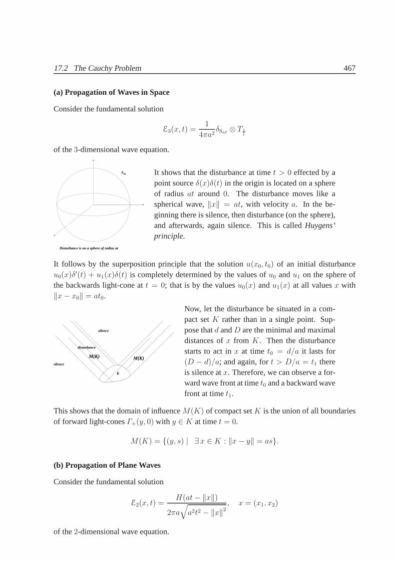
17.2 The Cauchy Problem 467
(a) Propagation of Waves in Space
Consider the fundamental solution
E3(x, t) =1
4πa2δSat ⊗ T 1
t
of the3-dimensional wave equation.
Sat
Disturbance is on a sphere of radius at
It shows that the disturbance at timet > 0 effected by apoint sourceδ(x)δ(t) in the origin is located on a sphereof radius at around0. The disturbance moves like aspherical wave,‖x‖ = at, with velocity a. In the be-ginning there is silence, then disturbance (on the sphere),and afterwards, again silence. This is calledHuygens’principle.
It follows by the superposition principle that the solutionu(x0, t0) of an initial disturbanceu0(x)δ
′(t) + u1(x)δ(t) is completely determined by the values ofu0 andu1 on the sphere ofthe backwards light-cone att = 0; that is by the valuesu0(x) andu1(x) at all valuesx with‖x− x0‖ = at0.
K
silence
silence
disturbance
M(K) M(K)
Now, let the disturbance be situated in a com-pact setK rather than in a single point. Sup-pose thatd andD are the minimal and maximaldistances ofx from K. Then the disturbancestarts to act inx at time t0 = d/a it lasts for(D − d)/a; and again, fort > D/a = t1 thereis silence atx. Therefore, we can observe a for-ward wave front at timet0 and a backward wavefront at timet1.
This shows that the domain of influenceM(K) of compact setK is the union of all boundariesof forward light-conesΓ+(y, 0) with y ∈ K at timet = 0.
M(K) = (y, s) | ∃x ∈ K : ‖x− y‖ = as.
(b) Propagation of Plane Waves
Consider the fundamental solution
E2(x, t) =H(at− ‖x‖)
2πa√a2t2 − ‖x‖2
, x = (x1, x2)
of the2-dimensional wave equation.

468 17 PDE II — The Equations of Mathematical Physics
t=1 t=2 t=3
t=4
t=0
It shows that the disturbance effected by a pointsourceδ(x)δ(t) in the origin at time0 is a discUat of radiusat around0. One observes a for-ward wave front moving with speeda. In con-trast to the3-dimensional picture, there existsno back front. The disturbance is permanentlypresent fromt0 on. We speak of wavediffusion;Huygens’ principle does not hold.
Diffusion can also be observed in case of arbitrary initial disturbanceu0(x)δ′(t) + u1(x)δ(t).
Indeed, the superposition principle shows that the domain of dependence of a compact initialdisturbanceK is the union of all discsUat(y) with y ∈ K.
(c) Propagation on a Line
Recall thatE1(x, t) = 12aH(at − |x |). The disturbance at timet > 0 which is effected by a
point sourceδ(x)δ(t) is the whole closed interval[−at, at]. We have two forward wave “fronts”one at the pointx = at and one atx = −at; one moving to the right and one moving to the left.As in the plane case, there does not exist a back wave font; we observe diffusion.
For more details, see the discussion in Wladimirow, [Wla72,p. 155 – 159].
17.3 Fourier Method for Boundary Value Problems
A good, easy accessable introduction to the Fourier method is to be found in [KK71].
In this section we use Fourier series to solve BEVP to the Laplace equation as well as initialboundary value problems to the wave and heat equations.
Recall that the following sets are CNOS in the Hilbert spaceH
1√2π
eint | n ∈ Z, , H = L2(a, a + 2π),
1√b− a
e2πib−a
nt | n ∈ Z , H = L2(a, b),
1√2π,
1√π
sin(nt),1√π
cos(nt) | n ∈ N , H = L2(a, a+ 2π),
1√b− a
,
√2
b− a sin
(2π
b− a nt),
√2
b− a cos
(2π
b− a nt)| n ∈ N , H = L2(a, b),
For any functionf ∈ L1(0, 2π) one has an associated Fourier series
f ∼∑
n∈Z cn eint, cn =1√2π
∫ 2π
0
f(t)e−int dt.
17.3 Fourier Method for Boundary Value Problems 469
Lemma 17.14 Each of the following two sets forms a CNOS inH = L2(0, π) (on the halfinterval).
√2
πsin(nt) | n ∈ N , √
2
πcos(nt) | n ∈ N0
.
Proof. To check that they form an NOS is left to the reader. We show completeness of the firstset. Letf ∈ L2(0, π). Extendf to an odd functionf ∈ L2(−π, π), that isf(x) = f(x) andf(−x) = −f(x) for x ∈ (0, π). Sincef is an odd function, in its Fourier series
a0
2+
∞∑
n=1
an cos(nt) + bn sin(nt)
we havean = 0 for all n. Since the Fourier series∑∞
n=1 bn sin(nt) converges tof in L2(−π, π),it converges tof in L2(0, π). Thus, the sine system is complete. The proof for the cosinesystem is analogous.
17.3.1 Initial Boundary Value Problems
(a) The Homogeneous Heat Equation, Periodic Boundary Conditions
We consider heat conduction in a closed wire loop of length2π. Let u(x, t) be the temperatureof the wire at positionx and timet. Since the wire is closed (a loop),u(x, t) = u(x + 2π, t);u is thought to be a2π periodic function onR for every fixedt. Thus, we have the followingperiodic boundary conditions
u(0, t) = u(2π, t), ux(0, t) = ux(2π, t), t ∈ R+. (PBC)
The initial temperature distribution at timet = 0 is given such that the BIVP reads
ut − a2uxx = 0, x ∈ R, t > 0,
u(x, 0) = u0(x), x ∈ R,(PBC).
(17.20)
Separation of variables.We are seeking solutions of the form
u(x, t) = f(x) · g(t)
ignoring the initial conditions for a while. The heat equation then takes the form
f(x)g′(t) = a2f ′′(x)g(t) ⇐⇒ 1
a2
g′(t)
g(t)=f ′′(x)
f(x)= κ = const.
We obtain the system of two independent ODE only coupled byκ:
f ′′(x)− κf(x) = 0, g′(t)− a2κg(t) = 0.
470 17 PDE II — The Equations of Mathematical Physics
The periodic boundary conditions imply:
f(0)g(t) = f(2π)g(t), f ′(x)g(t) = f ′′(2π)g(t)
which for nontrivialg givesf(0) = f(2π) andf ′(0) = f ′(2π). In caseκ = 0, f ′′(x) = 0 hasthe general solutionf(x) = ax + b. The only periodic solution isf(x) = b = const. Supposenow thatκ = −ν2 < 0. Then the general solution of the second order ODE is
f(x) = c1 cos(νx) + c2 sin(νx).
Sincef is periodic with period2π, only adiscreteset of valuesν are possible, namelyνn = n,n ∈ Z. This impliesκn = −n2, n ∈ N.Finally, in caseκ = ν2 > 0, the general solution
f(x) = c1eνx + c2e
−νx
provides no periodic solutionsf . So far, we obtained a set of solutions
fn(x) = an cos(nx) + bn sin(nx), n ∈ N0,
corresponding toκn = −n2. The ODE forgn(t) now reads
g′n(t) + a2n2gn(t) = 0.
Its solution isgn(t) = ce−a2n2t, n ∈ N. Hence, the solutions of the BVP are given by
un(x, t) = e−a2n2t(an cos(nx) + bn sin(nx)), n ∈ N, u0(x, t) =
a0
2
and finite or “infinite” linear combinations:
u(x, t) =a0
2+
∞∑
n=0
e−a2n2t(an cos(nx) + bn sin(nx)), (17.21)
Consider now the initial value, that ist = 0. The corresponding series is
u(x, 0) =a0
2+
∞∑
n=0
an cos(nx) + bn sin(nx), (17.22)
which gives the ordinary Fourier series ofu0(x). That is, the Fourier coefficientan andbn ofthe initial functionu0(x) formallygive a solutionu(x, t).
1. If the Fourier series ofu0 pointwise converges tou0, the initial conditions are satisfied bythe functionu(x, t) given in (17.21)
2. If the Fourier series ofu0 is twice differentiable (with respect tox), so is the functionu(x, t) given by (17.21).

17.3 Fourier Method for Boundary Value Problems 471
Lemma 17.15 Consider the BIVP(17.20). (a) Existence.Suppose thatu0 ∈ C4(R) is periodic.Then the functionu(x, t) given by(17.21)is in C2,1
x,t([0, 2π]×R+) and solves the classical BIVP(17.20).(b) Uniqueness and Stability.In the class of functionsC2,1
x,t([0, 2π] × R+) the solution of theabove BIVP is unique.
Proof. (a) The Fourier coefficients ofu(4)0 are bounded such that the Fourier coefficients ofu0
have growth1/n4 (integrate the Fourier series ofu(4)0 four times). Then the series foruxx(x, t)
andut(x, t) both are dominated by the series∞∑
n=0
1
n2; hence they converge uniformly. This
shows that the seriesu(x, t) can be differentiated term by term twice w.r.t.x and once w.r.t.t.(b) For any fixedt ≥ 0, u(x, t) is continuous inx. Considerv(t) := ‖u(x, t)‖2L2(0,2π). Then
v′(t) =d
dt
(∫ 2π
0
u(x, t)2 dx
)= 2
∫ 2π
0
u(x, t)ut(x, t) dx = 2
∫ 2π
0
u(x, t)a2uxx(x, t) dx
= 2
(a2ux u
∣∣2π0− a2
∫ 2π
0
(ux(x, t))2 dx
)= −2a2
∫ 2π
0
u2x dx ≤ 0.
This shows thatv(t) is monotonically decreasing int.Suppose nowu1 andu2 both solve the BIVP in the given class. Thenu = u1 − u2 solvesthe BIVP in this class with homogeneous initial values, thatis u(x, 0) = 0, hence,v(0) =
‖u(x, 0)‖2L2 = 0. Sincev(t) is decreasing fort ≥ 0 and non-negative,v(t) = 0 for all t ≥ 0;henceu(x, t) = 0 in L2(0, 2π) for all t ≥ 0. Sinceu(x, t) is continuous inx, this impliesu(x, t) = 0 for all x andt. Thus,u1(x, t) = u2(x, t)—the solution is unique.Stability. Sincev(t) is decreasing
supt∈R+
‖u(x, t)‖L2(0,2π) ≤ ‖u0‖L2(0,2π) .
This shows that small changes in the initial conditionsu0 imply small changes in the solutionu(x, t). The problem is well-posed.
(b) The Inhomogeneous Heat Equation, Periodic Boundary Conditions
We study the IBVP
ut − a2uxx = f(x, t),
u(x, 0) = 0,
(PBC).
(17.23)
Solution. Let en(x) = einx/√
2π, n ∈ Z, be the CNOS inL2(0, 2π). These functions are alleigen functions with respect to the differential operatord2
dx2 , e′′n(x) = −n2 en(x). Let t > 0 befixed and
f(x, t) ∼∑
n∈Z cn(t) en(x)

472 17 PDE II — The Equations of Mathematical Physics
be the Fourier series off(x, t) with coefficientscn(t). Foru, we try the following ansatz
u(x, t) ∼∑
n∈Z dn(t) en(x) (17.24)
If f(x, t) is continuous inx and piecewise continuously differentiable with respect tox, itsFourier series converges pointwise and we have
ut − a2uxx =∑
n∈Z (en d′(t) + a2n2end(t))
= f(x, t) =∑
n∈N cn(t)en.For eachn this is an ODE int
d′n(t) + a2n2dn(t) = cn(t), dn(0) = 0.
From ODE the solution is well-known
dn(t) = e−a2n2t
∫ t
0
ea2n2scn(s) ds.
Under certain regularity and growth conditions onf , (17.24) solves the inhomogeneous IBVP.
(c) The Homogeneous Wave Equation with Dirichlet Conditions
Consider the initial boundary value problem of the vibrating string of lengthπ.
(E) utt − a2uxx = 0, 0 < x < π, t > 0;
(BC) u(0, t) = u(π, t) = 0,
(IC) u(x, 0) = ϕ(x), ut(x, 0) = ψ(x), 0 < x < π.
The ansatzu(x, t) = f(x)g(t) yields
f ′′
f= κ =
g′′
a2g, f ′′(x) = κf(x), g′′ = κa2g.
The boundary conditions implyf(0) = f(π) = 0. Hence, the first ODE has the only solutions
fn(x) = cn sin(nx), κn = −n2, n ∈ N.The corresponding ODEs forg then read
g′′n + n2a2gn = 0,
which has the general solutionan cos(nat) + bn sin(nat). Hence,
u(x, t) =∞∑
n=1
(an cos(nat) + bn sin(nat)) sin(nx)

17.3 Fourier Method for Boundary Value Problems 473
solves the boundary value problem in the sense ofD′(R2) (choose anyan, bn of polynomialgrowth). Now, insert the initial conditions,t = 0:
u(x, 0) =
∞∑
n=1
an sin(nx)!= ϕ(x), ut(x, 0) =
∞∑
n=1
nabn sin(nx)!= ψ(x).
Since√
2π
sin(nx) | n ∈ N is a CNOS inL2(0, π), we can determine the Fourier coefficientsof ϕ andψ with respect to this CNOS and obtainan andbn, respectively.Regularity. Suppose thatϕ ∈ C4([0, π]), ψ ∈ C3([0, π]). Then the Fourier-Sine coefficientsanandanbn of ϕ andψ have growth1/n4 and1/n3, respectively. Hence, the series
u(x, t) =
∞∑
n=1
(an cos(nat) + bn sin(nat)) sin(nx) (17.25)
can be differentiated twice with respect tox or t since the differentiated series have a summableupper bound
∑c/n2. Hence, (17.25) solves the IBVP.
(d) The Wave Equation with Inhomogeneous Boundary Conditions
Consider the following problem inΩ ⊂ Rn
utt − a2∆u = 0,
u(x, 0) = ut(x, 0) = 0
u |∂Ω = w(x, t).
Idea.Find an extensionv(x, t) of w(x, t), v ∈ C2(Ω ×R+), and look for functionsu = u− v.Thenu has homogeneous boundary conditions and satisfies the IBVP
utt − a2∆u = −vtt + a2∆v,
u(x, 0) = −v(x, 0), ut(x, 0) = −vt(x, 0)
u |∂Ω = 0.
This problem can be split into two problems, one with zero initial conditions and one withhomogeneous wave equation.
17.3.2 Eigenvalue Problems for the Laplace Equation
In the previous subsection we have seen that BIVPs using Fourier’s method often lead to bound-ary eigenvalue problems (BEVP) for the Laplace equation.We formulate the problems. Letn = 1 andΩ = (0, l). One considers the following types ofBEVPs to the Laplace equation;f ′′ = λf :
• Dirichlet boundary conditions:f(0) = f(l) = 0.
• Neumann boundary conditions:f ′(0) = f ′(l) = 0.

474 17 PDE II — The Equations of Mathematical Physics
• Periodic boundary conditions :f(0) = f(l), f ′(0) = f ′(l).
• Mixed boundary conditions:α1f(0) + α2f′(0) = 0, β1f(l) + β2f
′(l) = 0.
• Symmetric boundary conditions: Ifu andv are function satisfying these boundary condi-tions, then(u′v − uv′)|l0 = 0. In this case integration by parts gives
∫ l
0
(u′′v − uv′′) dx = u′v − v′u|l0 −∫ l
0
(u′v′ − v′u′) dx = 0.
That isu′′·v = u·v′′ and the Laplace operator becomes symmetric.
Proposition 17.16 LetΩ ⊂ Rn. The BEVP with Dirichlet conditions
∆u = λu, u |∂Ω= 0, u ∈ C2(Ω) ∩ C1(Ω) (17.26)
has countably many eigenvaluesλk. All eigenvalues are negative and of finite multiplicity. Let0 > λ1 > λ2 > · · · then sequence( 1
λk) tends to0. The eigenfunctionsuk corresponding toλk
form a CNOS inL2(Ω).
Sketch of proof.(a) LetH = L2(Ω). We use Green’s1st formula withu = v , u |∂Ω= 0,∫
Ω
u∆u dx+
∫
Ω
(∇u)2 dx = 0.
to show that all eigenvalues of∆ are negative. Let∆u = λu. First note, thatλ = 0 is not aneigenvalue of∆. Suppose to the contrary∆u = 0, that is,u is harmonic. Sinceu |∂Ω= 0, bythe uniqueness theorem for the Dirichlet problem,u = 0 in Ω. Then
λ ‖u‖2 = λ 〈u , u〉 = 〈λu , u〉 = 〈∆u , u〉 =∫
Ω
u∆u dx = −∫
Ω
(∇u)2 dx < 0.
Hence,λ is negative.(b) Assume that a Green’s functionG for Ω exists. By (17.34), that is
u(y) =
∫
Ω
G(x, y) ∆u(x) dx+
∫
∂Ω
u(x)∂G(x, y)
∂~nxdS(x),
u |∂Ω= 0 implies
u(y) =
∫
Ω
G(x, y) ∆u(x) dx.
This shows that the integral operatorA : L2(Ω)→ L2(Ω) defined by
(Av)(y) :=
∫
Ω
G(x, y)v(x) dx
is inverse to the Laplacian. SinceG(x, y) = G(y, x) is real,A is self-adjoint. By (a), itseigenvalues,1/λk are all negative. If
∫∫
Ω×Ω
|G(x, y) |2 dxdy <∞,

17.3 Fourier Method for Boundary Value Problems 475
A is acompactoperator.We want to justify the last statement. Let(Kf)(x) =
∫Ωk(x, y)f(y) dy be an integral operator
onH = L2(Ω), with kernelk(x, y) ∈ H = L2(Ω × Ω). Let un | n ∈ N be a CNOS inH;thenun(x)um(y) | n,m ∈ N is a CNOS inH. Let knm be the Fourier coefficients ofk withrespect to the basisun(x)um(y) in H. Then
(Kf)(x) =
∫
Ω
f(y)∑
n,m
knmun(x)um(y) dy
=∑
n
un(x)
(∑
m
knm
∫
Ω
um(y)f(y) dy
)
=∑
n
un(x)∑
m
knm 〈f , um〉 =∑
n,m
knm 〈f , um〉 un.
This in particular shows that
‖Kf‖2 =∑
m,n
k2mn 〈f , um〉2 ≤
∑
m,n
k2mn ‖f‖2 = ‖f‖2
∫
Ω×Ωk(x, y)2 dxdy = ‖f‖2
∑
n
‖Kun‖2
‖K‖2 ≤∑
n
‖Kun‖2
We show thatK is approximated by the sequence(Kn) defined by
Kn f =∑
m
n∑
r=1
krm 〈f , um〉 ur
of finite rank operators. Indeed,
‖(K −Kn)f‖2 =∑
m
∞∑
r=n+1
k2rm | 〈f , um〉 |2 ≤ sup
m
∞∑
r=n+1
k2rm ‖f‖2
such that
‖K −Kn‖2 = supm
∞∑
r=n+1
k2rm −→ 0
asn→∞. Hence,K is compact.(c) By (a) and (b),A is a negative, compact, self-adjoint operator. By the spectral theorem forcompact self-adjoint operators, Theorem 13.33, there exists an NOS(uk) of eigenfunctions to1/λk of A. The NOS(uk) is complete since0 is not an eigenvalue ofA.
Example 17.1 Dirichlet Conditions on the Square.Let Q = (0, π) × (0, π) ⊂ R2. TheLaplace operator with Dirichlet boundary conditions onΩ has eigenfunctions
umn(x, y) =2
πsin(mx) sin(ny),
corresponding to the eigenvaluesλmn = −(m2 + n2). The eigenfunctionsumn | m,n ∈ Nform a CNOS in the Hilbert spaceL2(Ω).

476 17 PDE II — The Equations of Mathematical Physics
Example 17.2 Dirichlet Conditions on the ball U1(0) in R2. We consider the BEVP withDirichlet boundary conditions on the ball.
−∆u = λu, u |S1(0)= 0.
In polar coordinatesu(x, y) = u(r, ϕ) this reads,
∆u(r, ϕ) =1
r
∂
∂r(r ur) +
1
r2uϕϕ = −λu, 0 < r < 1, 0 ≤ ϕ < 2π.
Separation of variables.We try the ansatzu(r, ϕ) = R(r)Φ(ϕ). We have the boundary condi-tionR(1) = 0 and inR(r) is bounded in a neighborhood ofr = 0. Also,Φ is periodic. Then∂∂ru = R′Φ and
∂
∂r(rur) =
∂
∂r(rR′Φ) = (R′ + rR′′)Φ, uϕϕ = RΦ′′.
Hence,∆u = −λu now reads(R′
r+R′′
)Φ +
R
r2Φ′′ = −λRΦ
R′
r+R′′
R+
1
r2
Φ′′
Φ= −λ
rR′ + r2R′′
R+ λr2 = −Φ
′′
Φ= µ.
In this way, we obtain the two one-dimensional problems
Φ′′ + µΦ = 0, Φ(0) = Φ(2π);
r2R′′ + rR′ + (λr2 − µ)R = 0, |R(0) | <∞, R(1) = 0. (17.27)
The eigenvalues and eigenfunctions to the first problem are
µk = k2, Φk(ϕ) = eikϕ, k ∈ Z.Equation (17.27) is the Bessel ODE. Forµ = k2 the solution of (17.27) bounded inr = 0 isgiven by the Bessel functionJk(r
√λ). Recall from homework 21.2 that
Jk(x) =
∞∑
n=0
(−1)n(x2
)2n+k
n!(n + k)!, k ∈ N0.
To determine the eigenvaluesλ we use the boundary conditionR(1) = 0 in (17.27), namelyJk(√λ) = 0. Hence,
√λ = µkj, whereµkj, j = 1, 2, . . . , denote the positive zeros ofJk. We
obtainλkj = µ2
kj, Rkj(r) = Jk(µkj r), j = 1, 2, · · · .The solution of the BEVP is
λkj = µ2kj, ukj(x) = J| k |(µ| k |jr)e
ikϕ, k ∈ Z, j = 1, 2, · · · .
Note that the Bessel functionsJk | k ∈ Z+ and the systemeikt | k ∈ Z form a completeOS inL2((0, 1), r dr) and in inL2(0, 2π), respectively. Hence, the OSukl | k ∈ Z, l ∈ Z+ isa complete OS inL2(U1(0)). Thus, there are no further solutions to the given BEVP. For moredetails on Bessel functions, see [FK98, p. 383].

17.4 Boundary Value Problems for the Laplace and the PoissonEquations 477
17.4 Boundary Value Problems for the Laplace and the Pois-son Equations
Throughout this section (if nothing is stated otherwise) wewill assume thatΩ is a boundedregion inRn, n ≥ 2. We suppose further thatΩ belongs to the classC2, that is, the boundary∂Ω consists of finitely many twice continuously differentiable hypersurfaces;Ω′ := Rn \Ω isassumed to be connected (i. e. it is a region, too). All functions are assumed to be real valued.
17.4.1 Formulation of Boundary Value Problems
(a) The Inner Dirichlet Problem:
Givenϕ ∈ C(∂Ω) andf ∈ C(Ω), find u ∈ C(Ω) ∩ C2(Ω) such that
∆u(x) = f(x) ∀x ∈ Ω, and
u(y) = ϕ(y), ∀ y ∈ ∂Ω.
(b) The Exterior Dirichlet Problem:
Givenϕ ∈ C(∂Ω) andf ∈ C(Ω′), find u ∈ C(Ω′) ∩ C2(Ω′) such that
∆u(x) = f(x), ∀x ∈ Ω′, and
u(y) = ϕ(y), ∀ y ∈ ∂Ω,lim
|x |→∞u(x) = 0.
(c) The Inner Neumann Problem:
y
Ω
x=y−tn
n
Givenϕ ∈ C(∂Ω) andf ∈ C(Ω), find u ∈ C1(Ω) ∩ C2(Ω)
such that
∆u(x) = f(x) ∀x ∈ Ω, and
∂u
∂~n−(y) = ϕ(y), ∀ y ∈ ∂Ω.
Here ∂u∂~n−
(y) denotes the limit of directional derivative
∂u
∂~n−(y) = lim
t→0+0~n(y) · grad u(y − t~n(y))
and~n(y) is the outer normal toΩ aty ∈ ∂Ω. That is,x ∈ Ω approachesy ∈ ∂Ω in the directionof the normal vector~n(y). We assume that this limit exists for all boundary pointsy ∈ ∂Ω.

478 17 PDE II — The Equations of Mathematical Physics
(d) The Exterior Neumann Problem:
y
Ω
n
x=y+tn
Givenϕ ∈ C(∂Ω) andf ∈ C(Ω′), find u ∈ C1(Ω′) ∩C2(Ω′) such that
∆u(x) = f(x) ∀x ∈ Ω′, and
∂u
∂~n+(y) = ϕ(y), ∀ y ∈ ∂Ω
lim|x |→∞
u(x) = 0.
Here ∂u∂~n+
(y) denotes the limit of directional derivative
∂u
∂~n+(y) = lim
t→0+0~n(y) · gradu(y + t~n(y))
and~n(y) is the outer normal toΩ at y ∈ ∂Ω. We assume that this limit exists for all boundarypointsy ∈ ∂Ω. In both Neumann problems one can also look for a functionu ∈ C2(Ω)∩C(Ω)
or u ∈ C2(Ω′) ∩ C(Ω′), respectively, provided the above limits exist and define continuous
functions on the boundary.These four problems are intimately connected with each other, and we will obtain solutions toall of them simultaneously.
17.4.2 Basic Properties of Harmonic Functions
Recall that a functionu ∈ C2(Ω), is said to beharmonicif ∆u = 0 in Ω.We say that an operatorL on a function spaceV overRn is invariant under a affine transfor-mationT , T (x) = A(x) + b, whereA ∈ L (Rn), b ∈ Rn, if
LT ∗ = T ∗L,
whereT ∗ : V → V is given by(T ∗f)(x) = f(T (x)), f ∈ V . It follows that the Laplacian isinvariant under translations (T (x) = x+b) and rotationsT (i. e. T⊤T = TT⊤ = I). Indeed, fortranslations, the matrixB with A = BAB⊤ is the identity and in case of the rotation,B = T−1.SinceA = I, in both cases,A = A = I; the Laplacian is invariant.In this section we assume thatΩ ⊂ Rn is a region where Gauß’ divergence theorem is valid forall vector fieldsf ∈ C1(Ω) ∩ C(Ω) for :
∫
Ω
div f(x) dx =
∫
∂Ω
f(y) · ~dS(y),
where the dot· denotes the inner product inRn. The term under the integral can be written as
ω(y) = f(y) · ~dS = (f1(y), · · · , fn(y)) · ( dy2 ∧ dy3 ∧ · · · ∧ dyn,− dy1 ∧ dy3 ∧ · · · ∧ dyn,
· · · , (−1)n−1 dy1 ∧ · · · ∧ dyn−1
)
=n∑
k=1
(−1)k−1fk(y) dy1 ∧ · · · ∧ dyk ∧ · · · ∧ dyn,

17.4 Boundary Value Problems for the Laplace and the PoissonEquations 479
where the hat means ommission of this factor. In this wayω(y) becomes a differential(n− 1)-form. Using differentiation of forms, see Definition 11.7, we obtain
dω = div f(y) dy1 ∧ dy2 ∧ · · · ∧ dyn.
This establishes the above generalized form of Gauß’ divergence theorem. LetU : ∂Ω → R bea continuous scalar function on∂Ω, one can defineU(y) dS(y) := U(y)~n(y) · ~dS(y), where~nis the outer unit normal vector to the surface∂Ω.Recall that we obtain Green’s first formula insertingf(x) = v(x)∇u(x), u, v ∈ C2(Ω):
∫
Ω
v(x)∆u(x) dx+
∫
Ω
∇u(x) · ∇v(x) dx =
∫
∂Ω
v(y)∂u
∂~n(y) dS(y).
Interchanging the role ofu andv and taking the difference, we obtain Green’s second formula∫
Ω
(v(x)∆u(x)− u(x)∆v(x)) dx =
∫
∂Ω
(v(y)
∂u
∂~n(y)− u(y)∂v
∂~n(y)
)dS(y). (17.28)
Recall that
E2(x) =1
2πlog ‖x‖ , n = 2,
En(x) = − 1
(n− 2)ωn‖x‖−n+2 , n ≥ 3
are the fundamental solutions of the Laplacian inRn.
Theorem 17.17 (Green’s representation formula)Letu ∈ C2(Ω).Then forx ∈ Ω we have
u(x) =
∫
Ω
En(x− y) ∆u(y) dy +
∫
∂Ω
(u(y)
∂En∂~ny
(x− y)− En(x− y)∂u
∂~n(y)
)dS(y)
(17.29)
Here ∂∂~ny
denotes the derivative in the direction of the outer normal with respect to the variabley.
Note that the distributions∆u,(∂u∂~nδ∂Ω), and ∂
∂~n(u δ∂Ω) have compact support such that the
convolution products withEn exist.Proof. Idea of proofFor sufficiently smallε > 0, Uε(x) ⊂ Ω, sinceΩ is open. We applyGreen’s second formula withv(y) = En(x − y) andΩ \Uε(x) in place ofΩ. SinceEn(x − y)is harmonic with respect to the variabley in Ω \ x (recall from Example 7.5, thatEn(x) isharmonic inRn \ 0), we obtain
∫
Ω \Uε(x)
En(x− y)∆(y) dy =
∫
∂Ω
(En(x− y)
∂u
∂~n(y)− u(y)∂En(x− y)
∂~ny
)dS(y)
+
∫
∂Uε(x)
(En(x− y)
∂u
∂~n(y)− u(y)∂En(x− y)
∂~ny
)dS(y). (17.30)

480 17 PDE II — The Equations of Mathematical Physics
In the second integral~n denotes the outer normal toΩ \Uε(x) hence the inner normal ofUε(x).We wish to evaluate the limits of the individual integrals inthis formula asε → 0. Considerthe left-hand side of (17.30). Sinceu ∈ C2(Ω), ∆u is bounded; sinceEn(x − y) is locallyintegrable, the lhs converges to
∫
Ω
En(x− y) ∆u(y) dy.
On∂Uε(x), we haveEn(x− y) = βnε−n+2, βn = −1/(ωn(n− 2)). Thus asε→ 0,
∣∣∣∣∣∣∣
∫
∂Uε(x)
En(x− y)∂u
∂~n(y) dS
∣∣∣∣∣∣∣≤ |βn |εn−2
∫
∂Uε(x)
∣∣∣∣∂u
∂~n(y)
∣∣∣∣ dS ≤ |βn |εn−2
supUε(x)
∣∣∣∣∂u(y)
∂~n
∣∣∣∣∫
Sε(x)
dS
≤ 1
(n− 2)ωnεn−2ωnε
n−1 supUε(x)
∣∣∣∣∂u(y)
∂~n
∣∣∣∣ = Cε −→ 0.
Furthermore, since~n is the interior normal of the ballUε(y), the same calculations as in theproof of Theorem 17.1 show that∂En(x−y)
∂~ny= −βn d
dε(ε−n+2) = −ε−n+1/ωn. We obtain,
−∫
∂Uε(x)
u(y)∂En(x− y)
∂~nydS(y) =
1
ωnεn−1
∫
Sε(x)
u(y) dS(y)
︸ ︷︷ ︸spherical mean
−→ u(x).
In the last line we used that the integral is the mean value ofu over the sphereSε(x), andu iscontinuous atx.
Remarks 17.4 (a) Green’s representation formula is also true for functionsu ∈ C2(Ω) ∩ C1(Ω). To prove this, consider Green’s representation theorem onsmallerregionsΩε ⊂ Ω such thatΩε ⊂ Ω.(b) Applying Green’s representation formula to a test function ϕ ∈ D(Ω), see Definition 16.1,ϕ(y) = ∂ϕ
∂~n(y) = 0, y ∈ ∂Ω, we obtain
ϕ(x) =
∫
Ω
En(x− y)∆ϕ(x) dx
(c) We may now draw the following consequence from Green’s representation formula: If oneknows∆u, thenu is completely determined by its values and those of its normal derivative on∂Ω. In particular, a harmonic function onΩ can be reconstructed from its boundary data. Onemay ask conversely whether one can construct a harmonic function for arbitrary given valuesof u and ∂u
∂~non ∂Ω. Ignoring regularity conditions, we will find out that this is not possible in
general. Roughly speaking, only one of these data is sufficient to describeu completely.(d) In case of a harmonic functionu ∈ C2(Ω)∩C1(Ω), ∆u = 0, Green’s representation formulareads (n = 3):
u(x) =1
4π
∫
∂Ω
(1
‖x− y‖∂u(y)
∂~n− u(y) ∂
∂~ny
1
‖x− y‖
)dS(y). (17.31)

17.4 Boundary Value Problems for the Laplace and the PoissonEquations 481
In particular, the surface potentialsV (0)(x) andV (1)(x) can be differentiated arbitrarily oftenfor x ∈ Ω. Outside∂Ω, V (0) andV (1) are harmonic. It follows from (17.31) that any harmonicfunction is aC∞-function.
Spherical Means and Ball Means
First of all note thatu ∈ C1(Ω) andu harmonic inΩ implies∫
∂Ω
∂u(y)
∂~ndS = 0. (17.32)
Indeed, this follows from Green’s first formula insertingv = 1 andu harmonic,∆u = 0.
Proposition 17.18 (Mean Value Property)Suppose thatu is harmonic inUR(x0) and contin-uous inUR(x0).(a)Thenu(x0) coincides with its spherical mean over the sphereSR(x0).
u(x0) =1
ωnRn−1
∫
SR(x0)
u(y) dS(y) (spherical mean). (17.33)
(b) Further,
u(x0) =n
ωnRn
∫
UR(x0)
u(x) dx (ball mean).
Proof. (a) For simplicity, we consider only the casen = 3 andx0 = 0. Apply Green’s repre-sentation formula (17.31) to any ballΩ = Uρ(0) with ρ < R. Noting (17.32) from (17.31) itfollows that
u(0) =1
4π
(1
ρ
∫
Sρ(0)
∂u(y)
∂~ndS −
∫
Sρ(0)
u(y)∂
∂~ny
1
‖y‖ dS
)
= − 1
4π
∫
Sρ(0)
u(y)∂
∂~ny
1
‖y‖ dS =1
4π
∫
Sρ(0)
u(y)1
ρ2dS
=1
4πρ2
∫
Sρ(0)
u(y) dS,
Sinceu is continuous on the closed ball of radiusR, the formula remains valid asρ→ R.(b) Use dx = dx1 · · · dxn = dr dSr where‖x‖ = r. Multiply both sides of (17.33) byrn−1 dr and integrate with respect tor from 0 toR:
∫ R
0
rn−1u(x0) dr =
∫ R
0
rn−1
(1
ωnrn−1
∫
SR(x0)
u(y) dS
)dr
1
nRnu(x0) =
1
ωn
∫
UR(x0)
u(x) dx.
The assertion follows. Note thatRnωn/n is exactly then-dimensional volume ofUR(x0). Theproof in casen = 2 is similar.

482 17 PDE II — The Equations of Mathematical Physics
Proposition 17.19 (Minimum-Maximum Principle) Letu be harmonic inΩ and continuousin Ω. Then
maxx∈Ω
u(x) = maxx∈∂Ω
u(x);
i. e. u attains its maximum on the boundary∂Ω. The same is true for the minimum.
Proof. Suppose to the contrary thatM = u(x0) = maxx∈Ω
u(x) is attained at an inner pointx0 ∈ ΩandM > m = max
x∈∂Ωu(x) = u(y0), y0 ∈ ∂Ω.
(a) We show thatu(x) = M is constant in any ballUε(x0) ⊂ Ω aroundx0.Suppose to the contrary thatu(x1) < M for somex1 ∈ Uε(x0). By continuity ofu, u(x) < M
for all x ∈ Uε(x0) ∩ Uη(x1). In particular
M = u(x0) =n
ωnεn
∫
Bε(x0)
u(x) dx <n
ωnεn
∫
Bε(x0)
M dy = M ;
this is a contradiction;u is constant inUε(x0).(b) u(x) = M is constant inΩ. Let x1 ∈ Ω; we will show thatu(x1) = M . SinceΩ isconnected and bounded, there exists a path fromx0 to x1 which can be covered by a chain offinitely many balls inΩ. In all balls, starting with the ball aroundx0 from (a),u(x) = M isconstant. Hence,u is constant inΩ. Sinceu is continuous,u is constant inΩ. This contradictsthe assumption; hence, the maximum is assumed on the boundary ∂Ω.Passing fromu to−u, the statement about the minimum follows.
Remarks 17.5 (a) A stronger proposition holds with “local maximum” in place of “maximum”(b) Another stricter version of the maximum principle is:
Let u ∈ C2(Ω) ∩ C(Ω) and∆u ≥ 0 in Ω. Then eitheru is constant or
u(y) < maxx∈∂Ω
u(x)
for all y ∈ Ω.
Corollary 17.20 (Uniqueness)The inner and the outer Dirichlet problem has at most one so-lution, respectively.
Proof. Suppose thatu1 andu2 both are solutions of the Dirichlet problem,∆u1 = ∆u2 = f .Putu = u1 − u2. Then∆u(x) = 0 for all x ∈ Ω andu(y) = 0 on the boundaryy ∈ ∂Ω.(a) Inner problem. By the maximum principle,u(x) = 0 for all x ∈ Ω; that isu1 = u2.
Ω
B(0)r
(b) Suppose thatu 6≡ 0. Without loss of generality we may assume thatu(x1) = α > 0 for somex1 ∈ Ω′. By assumption,|u(x) | → 0 asx → ∞. Hence, there existsr > 0 such that| u(x) | < α/2 for allx ≥ r. Sinceu is harmonic inBr(0) \Ω, the maximum principle yields
α = u(x1) ≤ maxx∈SR(0)∪∂Ω
u(x) ≤ α/2;
a contradiction.

17.4 Boundary Value Problems for the Laplace and the PoissonEquations 483
Corollary 17.21 (Stability) Suppose thatu1 andu2 are solutions of the inner Dirichlet prob-lem ∆u1 = ∆u2 = f with boundary valuesϕ1(y) andϕ2(y) on ∂Ω, respectively. Supposefurther that
|ϕ1(y)− ϕ2(y) | ≤ ε ∀ y ∈ ∂Ω.
Then|u1(x)− u2(x) | ≤ ε for all x ∈ Ω.
A similar statement is true for the exterior Dirichlet problem.Proof. Putu = u1 − u2. Then∆u = 0 and |u(y) | ≤ ε for all y ∈ ∂Ω. By the MaximumPrinciple,| u(x) | ≤ ε for all x ∈ Ω.
Lemma 17.22 Suppose thatu is a non-constantharmonic function onΩ and the maximum ofu(x) is attained aty ∈ ∂Ω.Then∂u
∂~n(y) > 0.
For the proof see [Tri92, 3.4.2. Theorem, p. 174].
Proposition 17.23 (Uniqueness)(a)The exterior Neumann problem has at most one solution.(b) A necessary condition for solvability of the inner Neumann problem is
∫
∂Ω
ϕ dS =
∫
Ω
f(x) dx.
Two solutions of the inner Neumann problem differ by a constant.
Proof. (a) Suppose thatu1 andu2 are solutions of the exterior Neumann problem, thenu =
u1 − u2 satisfies∆u = 0 and∂u
∂~n(y) = 0. The above lemma shows thatu(x) = c is constant in
Ω. Sincelim|x |→∞ u(x) = 0, the constantc is 0; henceu1 = u2.(b) Inner problem. The uniqueness follows as in (a). The necessity of the formula follows from(17.28) withv ≡ 1, ∆u = f , ∂v
∂~n= 0.
Proposition 17.24 (Converse Mean Value Theorem)Suppose thatu ∈ C(Ω) and that when-everx0 ∈ Ω such thatUr(x0) ⊂ Ω we have the mean value property
u(x0) =1
ωnrn−1
∫
Sr(x0)
u(y) dS(y) =1
ωn
∫
S1(0)
u(x0 + ry) dS(y).
Thenu ∈ C∞(Ω) andu is harmonic inΩ.
Proof. (a) We show thatu ∈ C∞(Ω). The Mean Value Property ensures that the mollificationhε ∗ u equalsu as long asU1/ε(x0) ⊂ Ω; that is, the mollification does not changeu. By

484 17 PDE II — The Equations of Mathematical Physics
homework 49.4,u ∈ C∞ sincehε is. We provehε ∗ u = u. Hereg denotes the1-dimensionalbump function, see page 419.
uε(x) = (u ∗ hε)(x) =
∫Rn
u(y)hε(x− y) dy =
∫Rn
u(x− y)hε(y) dy
=
∫
Uε(0)
u(x− y)h(y/ε)ε−n dy =zi=
yiε
∫
U1(0)
u(x− εz)h(z) dz
=
∫ 1
0
∫
S1(0)
u(x− rεy)g(r)rn−1 dS(y) dr
= ωnu(x)
∫ 1
0
g(r)rn−1 dr = u(x)
∫Rn
h(y) dy = u(x).
Second Part.Differentiating the above equation with respect tor yields∫Ur(x)
∆u(y) dy = 0
for any ball inΩ, since the left-hand sideu(x) does not depend onr.
0 =d
dr
∫
S1(0)
u(x+ ry) dS(y) =
∫
S1(0)
y · ∇u(x+ ry) dS(y)
=
∫
Sr(0)
(r−1z)∇u(x+ z)r1−n dS(z)
= r−n∫
Sr(0)
~n(z) · ∇u(x+ z) dS(z)
= r−n∫
Sr(0)
∂u
∂~n(x+ z) dS(z)
= r−n∫
Sr(x0)
∂u(y)
∂~ndS(y) = r−n
∫
Ur(x0)
∆u(x) dx.
In the last line we used Green’s2nd formula withv = 1. Thus∆u = 0. Suppose to the contrarythat∆u(x0) 6= 0, say∆u(x0) > 0. By continuity of∆u(x), ∆u(x) > 0 for x ∈ Uε(x0). Hence∫Uε(x0)
∆u(x) dx > 0 which contradicts the above equation. We conclude thatu is harmonic inUr(x0).
Remark 17.6 A regular distributionu ∈ D′(Ω) is calledharmonicif ∆u = 0, that is,
〈∆u , ϕ〉 =
∫
Ω
u(x) ∆ϕ(x) dx = 0, ϕ ∈ D(Ω).
Weyl’s Lemma: Any harmonic regular distribution is a harmonic function,in particular,u ∈C∞(Ω).
Example 17.3 Solve
∆u = −2, (x, y) ∈ Ω = (0, a)× (−b/2, b/2),
u |∂Ω = 0.

17.5 Appendix 485
Ansatz:u = w + v with ∆w = 0. For example, choosew = −x2 + ax. Then∆v = 0 withboundary conditions
v(0, y) = v(a, y) = 0, v(x,−b/2) = v(x, b/2) = x2 − ax.
Use separation of variables,u(x, y)) = X(x)Y (y) to solve the problem.
17.5 Appendix
17.5.1 Existence of Solutions to the Boundary Value Problems
(a) Green’s Function
Let u ∈ C2(Ω) ∩ C1(Ω). Let us combine Green’s representation formula and Green’s2nd formula with a harmonic functionv(x) = vy(x), x ∈ Ω, wherey ∈ Ω is thought to bea parameter.
u(y) =
∫
Ω
En(x− y) ∆u(x) dx+
∫
∂Ω
(u(x)
∂En∂~nx
(x− y)− En(x− y)∂u
∂~n(x)
)dS(x)
0 =
∫
Ω
vy(x)∆u(x) dx+
∫
∂Ω
(u(x)
∂vy∂~n
(x)− vy(x)∂u
∂~n(x)
)dS(x)
Adding up these two lines and denotingG(x, y) = En(x− y) + vy(x) we get
u(y) =
∫
Ω
G(x, y) ∆u(x) dx+
∫
∂Ω
(u(x)
∂G(x, y)
∂~nx−G(x, y)
∂u
∂~n(x)
)dS(x).
Suppose now thatG(x, y) vanishes for allx ∈ ∂Ω then the last surface integral is0 and
u(y) =
∫
Ω
G(x, y) ∆u(x) dx+
∫
∂Ω
u(x)∂G(x, y)
∂~nxdS(x). (17.34)
In the above formula,u is completely determined by its boundary values and∆u in Ω. Thismotivates the following definition.
Definition 17.4 A functionG : Ω ×Ω → R satisfying
(a)G(x, y) = 0 for all x ∈ ∂Ω, y ∈ Ω, x 6= y.(b) vy(x) = G(x, y)− En(x− y) is harmonic inx ∈ Ω for all y ∈ Ω.
is called aGreen’s functionof Ω. More precisely,G(x, y) is a Green’s function to the innerDirichlet problem onΩ.
Remarks 17.7 (a) The functionvy(x) is in particular harmonic inx = y. SinceEn(x− y) hasa pole atx = y, G(x, y) has a pole of the same order atx = y such thatG(x, y)− En(x − y)has no singularity.If such a functionG(x, y) exists, for allu ∈ C2(Ω) we have (17.34).

486 17 PDE II — The Equations of Mathematical Physics
In particular, if in addition,u is harmonic inΩ,
u(y) =
∫
∂Ω
u(x)∂G(x, y)
∂~nxdS(x). (17.35)
This is the so calledPoisson’s formula forΩ. In general, it is difficult to find Green’s function.For most regionsΩ it is even impossible to giveG(x, y) explicitely. However, ifΩ has kindof symmetry, one can use the reflection principle to construct G(x, y) explicitely. Nevertheless,G(x, y) exists for all “well-behaved”Ω (the boundary is aC2-set and Gauß’ divergence theoremholds forΩ).
(c) The Reflection Principle
This is a method to calculate Green’s function explicitely in case of domainsΩ with the follow-ing property: Using repeated reflections on spheres and on hyperplanes occurring as boundariesof Ω and its reflections, the wholeRn can be filled up without overlapping.
Example 17.4 Green’s function on a ballUR(0). For, we use the reflection on the sphereSR(0).Fory ∈ Rn put
O y y−
R
.
y :=
y R2
‖y‖2 , y 6= 0,
∞, y = 0.
Note that this map has the the propertyy · y = R2 and‖y‖2 y = R2y. Points on the sphereSR(0) are fix under this map,y = y. LetEn : R+ → R denote the corresponding toEn radialscalar function withE(x) = En(‖x‖), that isEn(r) = −1/((n − 2)ωnr
n−2), n ≥ 2. Then weput
G(x, y) =
En(‖x− y‖)− En
(‖y‖R‖x− y‖
), y 6= 0,
En(‖x‖)−En(R), y = 0.(17.36)
Forx 6= y,G(x, y) is harmonic inx, since for‖y‖ < R, ‖y‖ > R and thereforex− y 6= 0. ThefunctionG(x, y) has only one singularity inUR(0) namely atx = y and this is the same as thatof En(x− y). Therefore,
vy(x) = G(x, y)− En(x− y) =
−En
(‖y‖R‖x− y‖
), y 6= 0,
En(R), y = 0.

17.5 Appendix 487
is harmonic for allx ∈ Ω. Forx ∈ ∂Ω = SR(0) we have fory 6= 0
G(x, y) = En
((‖x‖2 + ‖y‖2 − 2x · y
)12
)−En
(‖y‖R
(‖x‖2 + ‖y‖2 − 2x · y
) 12
)
= En
((R2 + ‖y‖2 − 2x · y
)12
)−En
(‖y‖2 +
‖y‖2 ‖y‖2R2
− 2 ‖y‖2 x · yR2
) 12
= En
((R2 + ‖y‖2 − 2x · y
)12
)−En
((‖y‖2 +R2 − 2x · y
) 12
)= 0.
Fory = 0 we have
G(x, 0) = En(‖x‖)−En(R) = En(R)− En(R) = 0.
This proves thatG(x, y) is a Green’s function forUR(0). In particular, the above calculationshows thatr = ‖x− y‖ andr = ‖y‖
R‖x− y‖ are equal ifx ∈ ∂Ω.
One can show that Green’s function is symmetric, that isG(x, y) = G(y, x). This is a generalproperty of Green’s function.
To apply formula (17.34) we have to compute the normal derivative∂
∂~nxG(x, y). Note first that
for any constantz ∈ Rn andx ∈ SR(0)
∂
∂~nxf(‖x− z‖) = ~n · ∇f(‖x− z‖) =
x
‖x‖ · f′(‖x− z‖) x− z
‖x− z‖ .
Note further that for‖x‖ = R we have
r = ‖x− y‖ =‖y‖R‖x− y‖ , (17.37)
(x− y) · x− ‖y‖2
R2(x− y) · x = R2 − ‖y‖2 . (17.38)
Hence, fory 6= 0,
∂
∂~nxG(x, y) = − 1
(n− 2)ωn
(∂
∂~nx‖x− y‖−n+2 − ∂
∂~nx
(‖y‖−n+2
R−n+2‖x− y‖−n+2
))
=1
ωn
(‖x− y‖−n+1 x− y
‖x− y‖ ·x
‖x‖ −‖y‖−n+2
R−n+2‖x− y‖−n+1 x− y
‖x− y‖ ·x
‖x‖
)
=1
ωnrnR
((x− y) · x− (x− y)‖y‖
2
R2· x)
By (17.38), the expression in the brackets isR2 − ‖y‖2. Hence,
∂
∂~nxG(x, y) =
R2 − ‖y‖2ωnR
1
‖x− y‖n .
This formula holds true in casey = 0. Inserting this into (17.34) we have for any harmonicfunctionu ∈ C2(UR(0)) ∩ C(UR(0)) we have
u(y) =R2 − ‖y‖2ωnR
∫
SR(0)
u(x)
‖x− y‖n dS(x). (17.39)
This is the so calledPoisson’s formula for the ballUR(0).
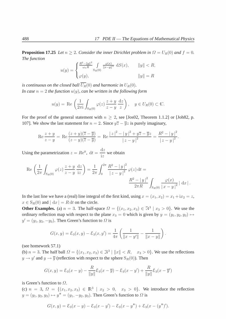
488 17 PDE II — The Equations of Mathematical Physics
Proposition 17.25 Letn ≥ 2. Consider the inner Dirichlet problem inΩ = UR(0) andf = 0.The function
u(y) =
R2−‖y‖2
ωnR
∫SR(0)
ϕ(x)‖x−y‖n dS(x), ‖y‖ < R,
ϕ(y), ‖y‖ = R
is continuous on the closed ballUR(0) and harmonic inUR(0).In casen = 2 the functionu(y), can be written in the following form
u(y) = Re
(1
2πi
∫
SR(0)
ϕ(z)z + y
z − ydz
z
), y ∈ UR(0) ⊂ C.
For the proof of the general statement withn ≥ 2, see [Jos02, Theorem 1.1.2] or [Joh82, p.107]. We show the last statement forn = 2. Sinceyz − yz is purely imaginary,
Rez + y
z − y = Re(z + y)(z − y)(z − y)(z − y) = Re
| z |2 − | y |2 + yz − yz| z − y |2
=R2 − | y |2
| z − y |2.
Using the parametrizationz = Reit, dt =dz
izwe obtain
Re
(1
2π
∫
SR(0)
ϕ(z)z + y
z − ydz
iz
)=
1
2π
∫ 2π
0
R2 − | y |2
| z − y |2ϕ(z) dt =
R2 − | y |22πR
∫
SR(0)
ϕ(x)
|x− y |2| dx | .
In the last line we have a (real) line integral of the first kind, usingx = (x1, x2) = x1 +ix2 = z,x ∈ SR(0) and| dx | = R dt on the circle.Other Examples. (a) n = 3. The half-spaceΩ = (x1, x2, x3) ∈ R3 | x3 > 0. We use theordinary reflection map with respect to the planex3 = 0 which is given byy = (y1, y2, y3) 7→y′ = (y1, y2,−y3). Then Green’s function toΩ is
G(x, y) = E3(x, y)− E3(x, y′) =
1
4π
(1
‖x− y′‖ −1
‖x− y‖
).
(see homework 57.1)(b) n = 3. The half ballΩ = (x1, x2, x3) ∈ R3 | ‖x‖ < R, x3 > 0. We use the reflectionsy → y′ andy → y (reflection with respect to the sphereSR(0)). Then
G(x, y) = E3(x− y)−R
‖y‖E3(x− y)− E3(x− y′) +R
‖y‖E3(x− y′)
is Green’s function toΩ.(c) n = 3, Ω = (x1, x2, x3) ∈ R3 | x2 > 0, x3 > 0. We introduce the reflectiony = (y1, y2, y3) 7→ y∗ = (y1,−y2, y3). Then Green’s function toΩ is
G(x, y) = E3(x− y)− E3(x− y′)− E3(x− y∗) + E3(x− (y∗)′).

17.5 Appendix 489
Consider the Neumann problem and the ansatz for Green’s function in case of the Dirichletproblem:
u(y) =
∫
Ω
H(x, y) ∆u(x) dx+
∫
∂Ω
(u(x)
∂H(x, y)
∂~nx−H(x, y)
∂u
∂~n(x)
)dS(x). (17.40)
We want to choose a Green’s function of the second kindH(x, y) in such a way that only thelast surface integral remains present.Insertingu = 1 in the above formula, we have
1 =
∫
∂Ω
∂G(x, y)
∂~nxdS(x).
Imposing,∂G(x,y)∂~nx
= α = const. , this constant must beα = 1/vol(∂Ω).Note, that one defines a Green’s function to the Neumann problem replacingG(x, y) = 0 on∂Ω by the condition ∂
∂~nyG(x, y) = const.
Green’s function of second kind (Neumann problem) to the ball of radiusR in R3, UR(0).
H(x, y) = − 1
4π
(1
‖x− y‖ +R
‖y‖ ‖x− y‖ +1
Rlog
2R2
R2 − x · y + ‖y‖ ‖x− y‖
)
(c) Existence Theorems
The aim of this considerations is to sketch the method of proving existenceof solutions of thefour BVPs.Definition. Suppose thatΩ ⊂ Rn, n ≥ 3 and letµ(y) be a continuous function on the boundary∂Ω, that isµ ∈ C(∂Ω). We call
w(x) =
∫
∂Ω
µ(y) En(x− y) dS(y), x ∈ Rn, (17.41)
asingle-layer potentialand
v(x) =
∫
∂Ω
µ(y)∂En∂~n
(x− y) dS(y), x ∈ Rn (17.42)
adouble-layer potential
Remarks 17.8 (a) Forx 6∈ ∂Ω the integrals (17.41) and (17.42) exist.(b) The single layer potentialu(x) is continuous onRn. The double-layer potential jumps aty0 ∈ ∂Ω by µ(y0) asx approachesy0, see (17.43) below.
Theorem 17.26LetΩ be a connected bounded region inRn of the classC2 andΩ′ = Rn \Ω
also be connected.Then the interior Dirichlet problem to the Laplace equationhas a unique solution. It can berepresented in form of a double-layer potential. The exterior Neumann problem likewise has aunique solution which can be represented in form of a single-layer potential.

490 17 PDE II — The Equations of Mathematical Physics
Theorem 17.27Under the same assumptions as in the previous theorem, the inner Neumannproblem to the Laplace equation has a solution if and only if
∫∂Ωϕ(y) dS(y) = 0. If this
condition is satisfies, the solution is unique up to a constant.The exterior Dirichlet problem has a unique solution.
Remark. LetµID denote the continuous functions which produces the solution v(x) of the inte-
rior Dirichlet problem, i. e.v(x) =∫∂ΩµID(y)K(x, y) dS(y), whereK(x, y) =
∂
∂~nyEn(x−y).
Because of the jump relation forv(x) atx0 ∈ ∂Ω:
limx→x0,x∈Ω
v(x)− 1
2µ(x0) = v(x0) = lim
x→x0,x∈Ω′v(x) +
1
2µ(x0), (17.43)
µID satisfies the integral equation
ϕ(x) =1
2µID(x) +
∫
∂Ω
µID(y)K(x, y) dS(y), x ∈ ∂Ω.
The above equation can be written asϕ = (A+ 12I)µID, whereA is the above integral operator
in L2(∂Ω). One can prove the following facts:A is compact,A+ 12I is injective and surjective,
ϕ continuous impliesµID continuous. For details, see [Tri92, 3.4].
Application to the Poisson Equation
Consider the inner Dirichlet problem∆u = f , andu = ϕ on ∂Ω. We suppose thatf ∈C(Ω) ∩ C1(Ω). We already know that
w(x) = (En ∗ f)(x) = − 1
(n− 2)ωn
∫Rn
f(y)
‖x− y‖n−2 dy
is a distributive solution of the Poisson equation,∆w = f . By the assumptions onf , w ∈C2(Ω) and therefore is a classical solution. To solve the problem we try the ansatzu = w + v.Then ∆u = ∆w + ∆v = f + ∆v. Hence,∆u = f if and only if ∆v = 0. Thus, theinner Dirichlet problem for the Poisson equation reduces tothe inner Dirichlet problem for theLaplace equation∆v = 0 with boundary values
v(y) = u(y)− w(y) = ϕ(y)− w(y) =: ϕ(y), y ∈ ∂Ω.
Sinceϕ andw are continuous on∂Ω, so isϕ.
17.5.2 Extremal Properties of Harmonic Functions and the DirichletPrinciple
(a) The Dirichlet Principle
Consider the inner Dirichlet problem to the Poisson equation with given dataf ∈ C(Ω) andϕ ∈ C(∂Ω).Put
C1ϕ(Ω) := v ∈ C1(Ω) | v = ϕ on ∂Ω.

17.5 Appendix 491
On this space define theDirichlet integralby
E(v) =1
2
∫
Ω
‖∇v‖2 dx+
∫
Ω
f · v dx, v ∈ C1ϕ(Ω). (17.44)
This integral is also calledenergy integral. The Dirichlet principle says that among all functionsv with given boundary valuesϕ, the functionu with ∆u = f minimizes the energy integralE.
Proposition 17.28 A functionu ∈ C1ϕ(Ω) ∩C2(Ω) is a solution of the inner Dirichlet problem
if and only if the energy integralE attains its minimum onC1ϕ(Ω) at u.
Proof. (a) Suppose first thatu ∈ C1ϕ(Ω) ∩ C2(Ω) is a solution of the inner Dirichlet problem,
∆u = f . Forv ∈ C1ϕ(Ω) letw = v − u ∈ C1
ϕ(Ω). Then
E(v) = E(u+ w) =1
2
∫
Ω
(∇u+∇w) · (∇u+∇w) dx+
∫
Ω
(u+ w)f dx
=1
2
∫
Ω
‖∇u‖2 +1
2
∫
Ω
‖∇w‖2 +
∫
Ω
∇u · ∇w dx+
∫
Ω
(u+ w)f dx
Sinceu andv satisfy the same boundary conditions,w |∂Ω= 0. Further,∆u = f . By Green’s1st formula,
∫
Ω
∇u · ∇w dx = −∫
Ω
(∆u)w dx+
∫
∂Ω
∂u
∂~nw dS = −
∫
Ω
f w dx.
Inserting this into the above equation, we have
E(v) =1
2
∫
Ω
‖∇u‖2 +1
2
∫
Ω
‖∇w‖2 −∫
Ω
fw dx+
∫
Ω
(u+ w)f dx
= E(u) +1
2
∫
Ω
‖∇w‖2 dx ≥ E(u).
This shows thatE(u) is minimal.(b) Conversely, letu ∈ C1
ϕ(Ω)∩C2(Ω) minimize the energy integral. In particular, for any testfunctionψ ∈ D(Ω), ψ has zero boundary values, the function
g(t) = E(u+ tψ) = E(u) + t
∫
Ω
(∇u · ∇ψ + fψ) dx+1
2t2∫
Ω
‖∇ψ‖2 dx
has a local minimum att = 0. Hence,g′(0) = 0 which is, again by Green’s1st formula andψ |∂Ω= 0, equivalent to
0 =
∫
Ω
(∇u · ∇ψ + fψ) dx =
∫
Ω
(−∆u + f) ψ dx.
By the fundamental Lemma of calculus of variations,∆u = f almost everywhere onΩ. Sinceboth∆u andf are continuous, this equation holds pointwise for allx ∈ Ω.

492 17 PDE II — The Equations of Mathematical Physics
(b) Hilbert Space Methods
We want to give another reformulation of the Dirichlet problem. Consider the problem
∆u = −f, u |∂Ω= 0.
OnC1(Ω) define a bilinear map
u·vE =
∫
Ω
∇u · ∇v dx.
C1(Ω) is not yet an inner product space since for any non-vanishingconstant functionu, u·uE =
0. Denote byC10(Ω) the subspace of functions inC1(Ω) vanishing on the boundary∂Ω. Now,
u·vE is an inner product onC10(Ω). The positive definiteness is a consequence of the Poincare
inequality below. Its corresponding norm is‖u‖2E =∫Ω‖∇u‖2 dx. Let u be a solution of the
above Dirichlet problem. Then for anyv ∈ C10(Ω), by Green’s1st formula
v·uE =
∫
Ω
∇v · ∇u dx = −∫
Ω
v∆u dx =
∫
Ω
v f dx = v·fL2.
This suggests thatu can be found by representing the known linear functional inv
F (v) =
∫
Ω
v f dx
as an inner productv·uE. To make use of Riesz’s representations theorem, Theorem 13.8, wehave to completeC1
0(Ω) into a Hilbert spaceW with respect to the energy norm‖·‖E and toprove that the above linear functionalF is bounded with respect to the energy norm. This isa consequence of the next lemma. We make the same assumtions onΩ as in the beginning ofSection 17.4.
Lemma 17.29 (Poincare inequality) LetΩ ⊂ Rn. Then there existsC > 0 such that for allu ∈ C1
0(Ω)
‖u‖L2(Ω) ≤ C ‖u‖E .
Proof. LetΩ be contained in the cubeΓ = x ∈ Rn | |xi | ≤ a, i = 1, . . . , n. We extenduby zero outsideΩ. For anyx = (x1, . . . , xn), by the Fundamental Theorem of Calculus
u(x)2 =
(∫ x1
−aux1(y1, x2, . . . , xn) dy1
)2
=
(∫ x1
−a1 · ux1(y1, x2, . . . , xn) dy1
)2
≤CSI
∫ x1
−ady1
∫ x1
−au2x1
dy1 = (x1 + a)
∫ x1
−au2x1
dy1 ≤ 2a
∫ a
−au2x1
dy1.
Since the last integral does not depend onx1, integration with respect tox1 gives∫ a
−au(x)2 dx1 ≤ 4a2
∫ a
−au2x1
dy1.
Integrating overx2, . . . , xn from−a to a we find∫
Γ
u2 dx ≤ 4a2
∫
Γ
u2x1
dy.

17.5 Appendix 493
The same inequality holds forxi, i = 2, . . . , n in place ofx1 such that
‖u‖2L2 =
∫
Γ
u2 dx ≤ 4a2
n
∫
Γ
(∇u)2 dx = C2 ‖u‖2E ,
whereC = 2a/√n.
The Poincare inequality is sometimes called Poincare–Friedrich inequality. It remains true forfunctionsu in the completionW . Let us discuss the elements ofW in more detail. By definition,f ∈ W if there is a Cauchy sequence(fn) in C1
0(Ω) such that(fn) “converges tof ” in theenergy norm. By the Poincare inequality,(fn) is also anL2-Cauchy sequence. SinceL2(Ω)
is complete,(fn) has anL2-limit f . This showsW ⊆ L2(Ω). For simplicity, letΩ ⊂ R1.By definition of the energy norm,
∫Ω| (fn − fm)′ |2 dx → 0, asm,n → ∞; that is(f ′
n) is anL2-Cauchy sequence, too. Hence,(f ′
n) has also someL2-limit, sayg ∈ L2(Ω). So far,
‖fn − f‖L2 −→ 0, ‖f ′n − g‖L2 −→ 0. (17.45)
We will show that the above limits implyf ′ = g in D′(Ω). Indeed, by (17.45) and the Cauchy–Schwarz inequality, for allϕ ∈ D(Ω),
∫
Ω
(fn − f)ϕ′ dx ≤(∫
Ω
| fn − f |2 dx
) 12(∫
Ω
|ϕ′ |2 dx
) 12
−→ 0,
∫
Ω
(f ′n − g)ϕ dx ≤
(∫
Ω
| f ′n − g |
2dx
) 12(∫
Ω
|ϕ |2 dx
) 12
−→ 0.
Hence,∫
Ω
f ′ ϕ dx = −∫
Ω
f ϕ′ dx = − limn→∞
∫
Ω
fn ϕ′ dx = lim
n→∞
∫
Ω
f ′n ϕ dx =
∫
Ω
g ϕ dx.
This showsf ′ = g in D′(Ω). One says that the elements ofW provideweak derivatives, thatis, its distributive derivative is anL2-function (and hence a regular distribution).Also, the inner product···E is positive definite since theL2-inner product is. It turns out thatWis a separable Hilbert space.W is the so calledSobolev spaceW1,2
0 (Ω) sometimes also denotedby H1
0(Ω). The upper indices1 and2 in W1,20 (Ω) refer to the highest order of partial derivatives
(|α | = 1) and theLp-space (p = 2) in the definition ofW , respectively. The lower index0refers to the so calledgeneralized boundary values0. For further readings on Sobolev spaces,see [Fol95, Chapter 6].
Corollary 17.30 F (v) = v·fL2 =∫Ωf v dx defines a bounded linear functional onW .
Proof. By the Cauchy–Schwarz and Poincare inequalities,
|F (v) | ≤∫
Ω
| f v | dx ≤ ‖f‖L2 ‖v‖L2 ≤ C ‖f‖L2 ‖v‖E .
Hence,F is bounded with‖F‖ ≤ C ‖f‖L2 .

494 17 PDE II — The Equations of Mathematical Physics
Corollary 17.31 Letf ∈ C(Ω). Then there exists a uniqueu ∈W such that
v·uE = v·fL2 , ∀ v ∈W.
Thisu solves
∆u = −f, in D′(Ω).
The first statement is a consequence of Riesz’s representation theorem; note thatF is a boundedlinear functional on the Hilbert spaceW . The last statement follows fromD(Ω) ⊂ C1
0(Ω) andu·ϕE = −〈∆u , ϕ〉 = f·ϕL2. This is the so calledmodified Dirichlet problem. It remains openthe task to identify the solutionu ∈W with anordinary functionu ∈ C2(Ω).
17.5.3 Numerical Methods
(a) Difference Methods
Since most ODE and PDE are not solvable in a closed form there are a lot of methods tofind approximative solutions to a given equation or a given problem. A general principle isdiscretization. One replaces the derivativeu′(x) by one of itsdifference quotients
∂+u(x) =u(x+ h)− u(x)
h, ∂−u(x) =
u(x)− u(x− h)h
,
whereh is called the step size. One can also use a symmetric difference u(x+h)−u(x−h)2h
. TheFive-Point formula for the Laplacian inR2 is then given by
∆hu(x, y) := (∂−x ∂+x + ∂−y ∂
+y )u(x, y) =
=u(x− h, y) + u(x+ h, y) + u(x, y − h) + u(x, y + h)− 4u(x, y)
h2
Besides the equation, the domainΩ as well as its boundary∂Ω undergo a discretization: IfΩ = (0, 1)× (0, 1) then
Ωh = (nh,mh) ∈ Ω | n,m ∈ N, ∂Ωh = (nh,mh) ∈ ∂Ω | n,m ∈ Z.The discretization of the inner Dirichlet problem then reads
∆hu = f, x ∈ Ωh,
u |∂Ωh= ϕ.
Also, Neumann problems have discretizations, [Hac92, Chapter 4].
(b) The Ritz–Galerkin Method
Suppose we have a boundary value problem in its variational formulation:
Findu ∈ V , so thatu·vE = F (v) for all v ∈ V ,

17.5 Appendix 495
where we are thinking of the Sobolev spaceV = W from the previous paragraph. Of course,F is assumed to be bounded.Difference methods arise through discretising the differential operator. Now we wish to leavethe differential operator which is hidden in···E unchanged. The Ritz–Galerkin method consistsin replacing the infinite-dimensional spaceV by a finite-dimensional spaceVN ,
VN ⊂ V, dim VN = N <∞.
VN equipped with the norm‖·‖E is still a Banach space. SinceVN ⊆ V , both the inner product···E andF are defined foru, v ∈ VN . Thus, we may pose the problem
FinduN ∈ VN , so thatuN·vE = F (v) for all v ∈ VN ,
The solution to the above problem, if it exists, is calledRitz–Galerkin solution(belonging toVN ).An introductory example is to be found in [Hac92, 8.1.11, p. 164], see also [Bra01, Chapter 2].

496 17 PDE II — The Equations of Mathematical Physics

Bibliography
[AF01] I. Agricola and T. Friedrich.Globale Analysis (in German). Friedr. Vieweg & Sohn,Braunschweig, 2001.
[Ahl78] L. V. Ahlfors. Complex analysis. An introduction to the theory of analyticfunc-tions of one complex variable. International Series in Pure and Applied Mathematics.McGraw-Hill Book Co., New York, 3 edition, 1978.
[Arn04] V. I. Arnold. Lectures in Partial Differential Equations. Universitext. Springer andPhasis, Berlin. Moscow, 2004.
[Bra01] D. Braess.Finite elements. Theory, fast solvers, and applications insolid mechanics.Cambridge University Press, Cambridge, 2001.
[Bre97] Glen E. Bredon.Topology and geometry. Number 139 in Graduate Texts in Mathe-matics. Springer-Verlag, New York, 1997.
[Bro92] Th. Brocker.Analysis II (German). B. I. Wissenschaftsverlag, Mannheim, 1992.
[Con78] J. B. Conway.Functions of one complex variable. Number 11 in Graduate Texts inMathematics. Springer-Verlag, New York, 1978.
[Con90] J. B. Conway.A course in functional analysis. Number 96 in Graduate Texts inMathematics. Springer-Verlag, New York, 1990.
[Cou88] R. Courant.Differential and integral calculus I–II. Wiley Classics Library. JohnWiley & Sons, New York etc., 1988.
[Die93] J. Dieudonne.Treatise on analysis. Volume I – IX. Pure and Applied Mathematics.Academic Press, Boston, 1993.
[Els02] J. Elstrodt.Maß- und Integrationstheorie. Springer, Berlin, third edition, 2002.
[Eva98] L. C. Evans.Partial differential equations. Number 19 in Graduate Studies in Math-ematics. AMS, Providence, 1998.
[FB93] E. Freitag and R. Busam.Funktionentheorie. Springer-Lehrbuch. Springer-Verlag,Berlin, 1993.
497

498 BIBLIOGRAPHY
[FK98] H. Fischer and H. Kaul.Mathematik fur Physiker. Band 2. Teubner Studienbucher:Mathematik. Teubner, Stuttgart, 1998.
[FL88] W. Fischer and I. Lieb.Ausgewahlte Kapitel der Funktionentheorie. Number 48 inVieweg Studium. Friedrich Vieweg & Sohn, Braunschweig, 1988.
[Fol95] G. B. Folland. Introduction to partial differential equations. Princeton UniversityPress, Princeton, 1995.
[For81] O. Forster. Analysis 3 (in German). Vieweg Studium: Aufbaukurs Mathematik.Vieweg, Braunschweig, 1981.
[For01] O. Forster.Analysis 1 – 3 (in German). Vieweg Studium: Grundkurs Mathematik.Vieweg, Braunschweig, 2001.
[GS64] I. M. Gelfand and G. E. Schilow.Verallgemeinerte Funktionen (Distributionen).III: Einige Fragen zur Theorie der Differentialgleichungen. (German). Number 49in Hochschulbucher fur Mathematik. VEB Deutscher Verlagder Wissenschaften,Berlin, 1964.
[GS69] I. M. Gelfand and G. E. Schilow.Verallgemeinerte Funktionen (Distributionen). I:Verallgemeinerte Funktionen und das Rechnen mit ihnen. (German). Number 47in Hochschulbucher fur Mathematik. VEB Deutscher Verlagder Wissenschaften,Berlin, 1969.
[Hac92] W. Hackbusch.Theory and numerical treatment. Number 18 in Springer Series inComputational Mathematics. Springer-Verlag, Berlin, 1992.
[Hen88] P. Henrici. Applied and computational complex analysis. Vol. 1. Wiley ClassicsLibrary. John Wiley & Sons, Inc., New York, 1988.
[How03] J. M. Howie. Complex analysis. Springer Undergraduate Mathematics Series.Springer-Verlag, London, 2003.
[HS91] F. Hirzebruch and W. Scharlau.Einfuhrung in die Funktionalanalysis. Number 296in BI-Hochschultaschenbucher. BI-Wissenschaftsverlag, Mannheim, 1991.
[HW96] E. Hairer and G. Wanner.Analysis by its history. Undergraduate texts in Mathematics.Readings in Mathematics. Springer-Verlag, New York, 1996.
[Jan93] K. Janich.Funktionentheorie. Springer-Lehrbuch. Springer-Verlag, Berlin, third edi-tion, 1993.
[Joh82] F. John.Partial differential equations. Number 1 in Applied Mathematical Sciences.Springer-Verlag, New York, 1982.
[Jos02] J. Jost.Partial differential equations. Number 214 in Graduate Texts in Mathematics.Springer-Verlag, New York, 2002.

BIBLIOGRAPHY 499
[KK71] A. Kufner and J. Kadlec.Fourier Series. G. A. Toombs Iliffe Books, London, 1971.
[Kno78] K. Knopp. Elemente der Funktionentheorie. Number 2124 in Sammlung Goschen.Walter de Gruyter, Berlin, New York, 9 edition, 1978.
[Kon90] K. Konigsberger.Analysis 1 (English). Springer-Verlag, Berlin, Heidelberg, NewYork, 1990.
[Lan89] S. Lang. Undergraduate Analysis. Undergraduate texts in mathematics. Springer,New York-Heidelberg, second edition, 1989.
[MW85] J. Marsden and A. Weinstein.Calculus. I, II, III. Undergraduate Texts in Mathemat-ics. Springer-Verlag, New York etc., 1985.
[Nee97] T. Needham.Visual complex analysis. Oxford University Press, New York, 1997.
[O’N75] P. V. O’Neil. Advanced calculus. Collier Macmillan Publishing Co., London, 1975.
[RS80] M. Reed and B. Simon.Methods of modern mathematical physics. I. FunctionalAnalysis. Academic Press, Inc., New York, 1980.
[Rud66] W. Rudin.Real and Complex Analysis. International Student Edition. McGraw-HillBook Co., New York-Toronto, 1966.
[Rud76] W. Rudin.Principles of mathematical analysis. International Series in Pure and Ap-plied Mathematics. McGraw-Hill Book Co., New York-Auckland-Dusseldorf, thirdedition, 1976.
[Ruh83] F. Ruhs.Funktionentheorie. Hochschulbucher fur Mathematik. VEB Deutscher Ver-lag der Wissenschaften, Berlin, 4 edition, 1983.
[Spi65] M. Spivak.Calculus on manifolds. W. A. Benjamin, New York, Amsterdam, 1965.
[Spi80] M. Spivak.Calculus. Publish or Perish, Inc., Berkeley, California, 1980.
[Str92] W. A. Strauss.Partial differential equations. John Wiley & Sons, New York, 1992.
[Tri92] H. Triebel. Higher analysis. Hochschulbucher fur Mathematik. Johann AmbrosiusBarth Verlag GmbH, Leipzig, 1992.
[vW81] C. von Westenholz.Differential forms in mathematical physics. Number 3 in Stud-ies in Mathematics and its Applications. North-Holland Publishing Co., Amsterdam-New York, second edition, 1981.
[Wal74] W. Walter.Einfuhrung in die Theorie der Distributionen (in German). Bibliographi-sches Institut, B.I.- Wissenschaftsverlag, Mannheim-Wien-Zurich, 1974.
[Wal02] W. Walter. Analysis 1–2 (in German). Springer-Lehrbuch. Springer, Berlin, fifthedition, 2002.

500 BIBLIOGRAPHY
[Wla72] V. S. Wladimirow.Gleichungen der mathematischen Physik (in German). Number 74in Hochschulbucher fur Mathematik. VEB Deutscher Verlagder Wissenschaften,Berlin, 1972.
PD DR. A. SCHULER
MATHEMATISCHES INSTITUT
UNIVERSITAT LEIPZIG
04009 LEIPZIG