Embed Size (px)
Citation preview
rspa.royalsocietypublishing.org
ResearchCite this article: DeVoria AC, Mohseni K. 2017A vortex model for forces and moments onlow-aspect-ratio wings in side-slip withexperimental validation. Proc. R. Soc. A 473:20160760.http://dx.doi.org/10.1098/rspa.2016.0760
Received: 7 October 2016Accepted: 27 January 2017
Subject Areas:fluid mechanics
Keywords:low-aspect-ratio wings, roll stall,high angle of attack
Author for correspondence:Kamran Mohsenie-mail: [email protected]
A vortex model for forces andmoments on low-aspect-ratiowings in side-slip withexperimental validationAdam C. DeVoria1 and Kamran Mohseni1,2
1Department of Mechanical and Aerospace Engineering, and2Department of Electrical and Computer Engineering,University of Florida, Gainesville, FL 32611, USA
KM, 0000-0002-1382-221X
This paper studies low-aspect-ratio (A) rectangularwings at high incidence and in side-slip. The mainobjective is to incorporate the effects of high angleof attack and side-slip into a simplified vortex modelfor the forces and moments. Experiments are alsoperformed and are used to validate assumptionsmade in the model. The model asymptotes to thepotential flow result of classical aerodynamics for aninfinite aspect ratio. TheA→ 0 limit of a rectangularwing is considered with slender body theory,where the side-edge vortices merge into a vortexdoublet. Hence, the velocity fields transition frombeing dominated by a spanwise vorticity monopole(A� 1) to a streamwise vorticity dipole (A∼ 1). Wetheoretically derive a spanwise loading distributionthat is parabolic instead of elliptic, and this physicallyrepresents the additional circulation around the wingthat is associated with reattached flow. This is afundamental feature of wings with a broad-facingleading edge. The experimental measurements of thespanwise circulation closely approximate a parabolicdistribution. The vortex model yields very agreeablecomparison with direct measurement of the lift anddrag, and the roll moment prediction is acceptable forA≤ 1 prior to the roll stall angle and up to side-slipangles of 20◦.
1. IntroductionThe recent interest in the applications of microaerialvehicles (MAVs) has led to a great deal of researchin several related areas, such as aerodynamic loading[1], flight control [2–4] and vehicle design [5]. Classical
2017 The Author(s) Published by the Royal Society. All rights reserved.
on February 22, 2017http://rspa.royalsocietypublishing.org/Downloaded from
2
rspa.royalsocietypublishing.orgProc.R.Soc.A473:20160760
...................................................
aerodynamic techniques and analyses are typically inapplicable to the low-Reynolds-numberflight regime in which most MAVs operate (5 × 10⁴–1 × 10⁵), which has impeded a thoroughunderstanding of the resulting aerodynamics. This is largely due to the fact that the flow fieldis inherently three-dimensional and often times unsteady, as well as being dominated by flowseparation and viscous effects. Furthermore, most MAVs consist of a lifting surface of lowaspect ratio (A), for which it is known that the effects of tip vortices (TVs) become increasinglyimportant. As a result, there is a complex interaction between the leading-edge separation region(LESR) and the TVs, which can affect the aerodynamic loads and flight characteristics.
A flight condition that is of considerable importance to low-A wings is side-slip. This isbecause these types of wings are susceptible to instability caused by disturbances. For example,a side-slip condition can be easily induced in an energetic environment by a slight windgust [6]. The complexity of low-A vehicle control stems from the sensitivity of their lateraldynamics. The fact that low-A wings have near-zero roll damping [4] amplifies the impact ofroll moments produced by lateral flow asymmetries. While a planar low-A rectangular wing isable to generate statically stable roll moments in side-slip (i.e. Cl,β < 0), the coupling betweenvortex lift and angle of attack results in an over-stabilizing dynamic derivative at increasedangles of attack. Shields & Mohseni [4] showed that for rectangular wings of sufficiently smallaspect ratio, such high levels of lateral stability, coupled with low roll damping, can result in anunder-damped dutch-roll-like stability mode. Additionally, angle of attack disturbances with afrequency similar to this mode can result in a divergent modal response that they termed ‘rollresonance’, and which couples the longitudinal and lateral dynamics. The lateral component issimilar to the well-known phenomenon of ‘wing rock’ observed to occur on free-to-roll deltawings [7,8] and to the self-induced oscillations of free-to-roll rectangular, elliptical, Zimmermanwings [9].
The majority of previous work on wings in side-slip has been applied to high aspect ratiosor to slender delta wings [10–12]. In this regard, Shields & Mohseni have conducted research onlow-A rectangular wings in side-slip [13–15]. Their static measurements showed the presenceof a few phenomena that they put under an umbrella term called ‘roll stall’. In this manuscript,the term roll stall refers specifically to the sudden decrease of the roll moment magnitude thatoccurs at a particular angle of attack, prior to which there is a monotonic increase with α; thisterminology is chosen based on the similar behaviour of the lift coefficient when lift stall occurs.The importance of roll stall on the flight dynamics of such a wing lies in the ability of a flightcontroller to accurately predict the actual control authority available. In other words, a linearcontroller will not be able to account for the rapid change in the Cl,α stability derivative associatedwith roll stall, and thus the wing could easily be sent into unstable flight. It should be noted thatLevin & Katz [7] found a very similar roll stall behaviour for slender delta wings, where theroll stall event occurs simultaneously with the lift or normal force stall. This happens, because thevortex lift of slender delta wings is due only to the two vortices generated along the highly sweptleading edges. However, inspection of the data of Shields & Mohseni reveals that, for rectangularwings, roll stall occurs well before lift stall for aspect ratios of unity and below. Moreover, low-A rectangular wings are different from delta wings in that there are three main wing edges andcorresponding vortices which interact to generate loads on the wing.
For delta wings, the aspect ratio is (by definition) uniquely determined from a singleparameter, namely the sweep angle Λ of the leading edges. Hence, a low-A delta wing is notnecessarily geometrically representative of other low-Awings that have more degrees of freedomin the planform definition. While the rolling dynamics of delta and rectangular wings, indeed,display similar traits, we believe that the different wing geometry is a fundamental differencethat leads to different flow physics and interactions that are responsible for the roll characteristics.The main purpose of this paper is to investigate the high angle of attack flow features of low-A rectangular wings in side-slip and to propose a simplified vortex model of the wings thatincorporates these features.
Although considerable understanding on roll stall of rectangular wings has been gained, thosestudies used global measurements, namely force balance data. In this paper, we obtain local
on February 22, 2017http://rspa.royalsocietypublishing.org/Downloaded from
3
rspa.royalsocietypublishing.orgProc.R.Soc.A473:20160760
...................................................
laser
mirror
plate
z
x
U
U
(a)
–b
a
cameras
Scheimpflugadapter lenses
laser sheet
y
x
(b)
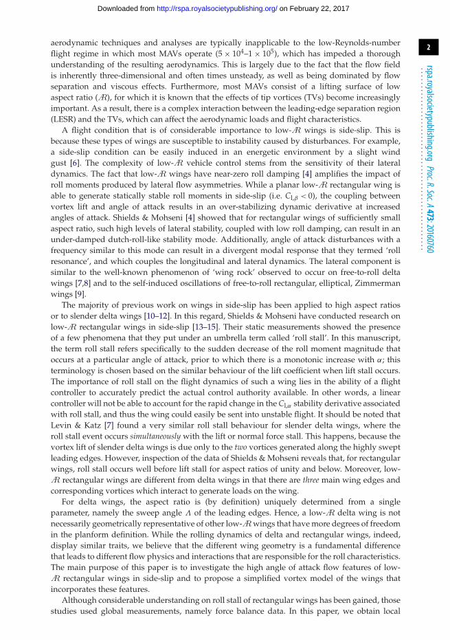
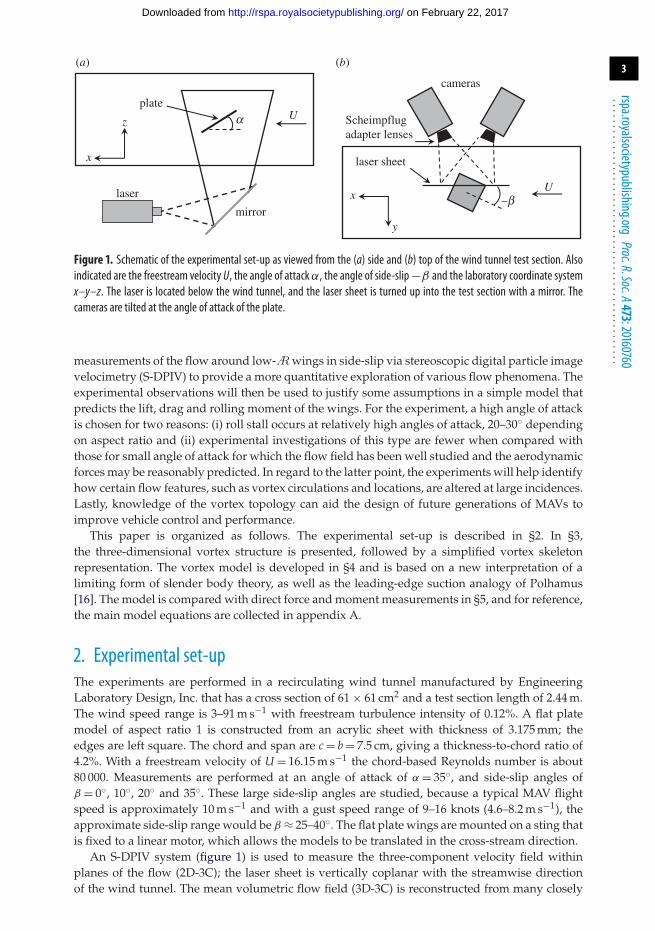
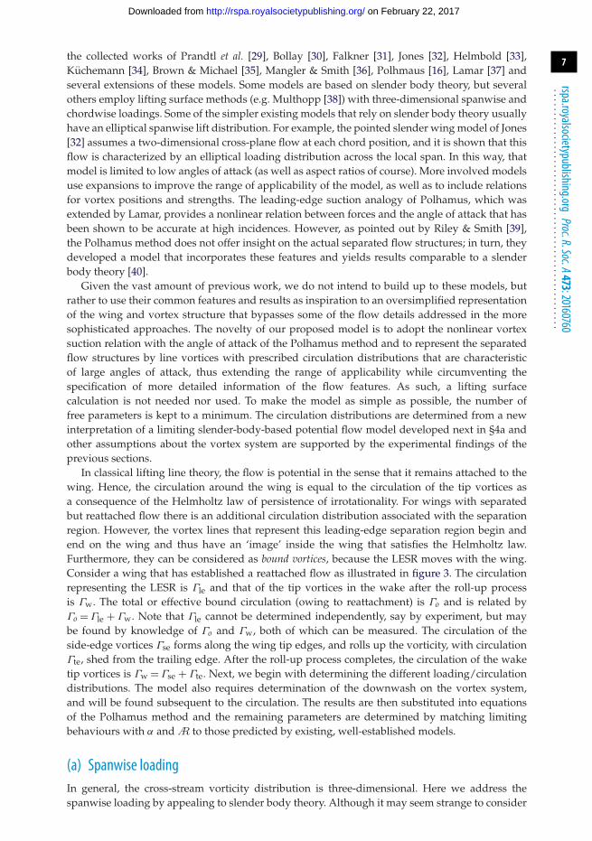
Figure 1. Schematic of the experimental set-up as viewed from the (a) side and (b) top of the wind tunnel test section. Alsoindicated are the freestream velocity U, the angle of attackα, the angle of side-slip−β and the laboratory coordinate systemx–y–z. The laser is located below the wind tunnel, and the laser sheet is turned up into the test section with a mirror. Thecameras are tilted at the angle of attack of the plate.
measurements of the flow around low-Awings in side-slip via stereoscopic digital particle imagevelocimetry (S-DPIV) to provide a more quantitative exploration of various flow phenomena. Theexperimental observations will then be used to justify some assumptions in a simple model thatpredicts the lift, drag and rolling moment of the wings. For the experiment, a high angle of attackis chosen for two reasons: (i) roll stall occurs at relatively high angles of attack, 20–30◦ dependingon aspect ratio and (ii) experimental investigations of this type are fewer when compared withthose for small angle of attack for which the flow field has been well studied and the aerodynamicforces may be reasonably predicted. In regard to the latter point, the experiments will help identifyhow certain flow features, such as vortex circulations and locations, are altered at large incidences.Lastly, knowledge of the vortex topology can aid the design of future generations of MAVs toimprove vehicle control and performance.
This paper is organized as follows. The experimental set-up is described in §2. In §3,the three-dimensional vortex structure is presented, followed by a simplified vortex skeletonrepresentation. The vortex model is developed in §4 and is based on a new interpretation of alimiting form of slender body theory, as well as the leading-edge suction analogy of Polhamus[16]. The model is compared with direct force and moment measurements in §5, and for reference,the main model equations are collected in appendix A.
2. Experimental set-upThe experiments are performed in a recirculating wind tunnel manufactured by EngineeringLaboratory Design, Inc. that has a cross section of 61 × 61 cm2 and a test section length of 2.44 m.The wind speed range is 3–91 m s−1 with freestream turbulence intensity of 0.12%. A flat platemodel of aspect ratio 1 is constructed from an acrylic sheet with thickness of 3.175 mm; theedges are left square. The chord and span are c = b = 7.5 cm, giving a thickness-to-chord ratio of4.2%. With a freestream velocity of U = 16.15 m s−1 the chord-based Reynolds number is about80 000. Measurements are performed at an angle of attack of α = 35◦, and side-slip angles ofβ = 0◦, 10◦, 20◦ and 35◦. These large side-slip angles are studied, because a typical MAV flightspeed is approximately 10 m s−1 and with a gust speed range of 9–16 knots (4.6–8.2 m s−1), theapproximate side-slip range would be β ≈ 25–40◦. The flat plate wings are mounted on a sting thatis fixed to a linear motor, which allows the models to be translated in the cross-stream direction.
An S-DPIV system (figure 1) is used to measure the three-component velocity field withinplanes of the flow (2D-3C); the laser sheet is vertically coplanar with the streamwise directionof the wind tunnel. The mean volumetric flow field (3D-3C) is reconstructed from many closely
on February 22, 2017http://rspa.royalsocietypublishing.org/Downloaded from
4
rspa.royalsocietypublishing.orgProc.R.Soc.A473:20160760
...................................................
spaced data planes, which is accomplished by laterally translating the plate through the lasersheet; in the worst-case scenario, the wing is still about 2.5 chords from the tunnel walls. The windtunnel is seeded with olive oil particles (approx. 1 µm) generated by an atomizer. Image pairs withan interframe time of �t = 50 µs are captured with 1 Mpx CMOS cameras (Phantom v.210/v.211,1280 × 800 px2) and illumination of the particles is provided by a 200 mJ Nd:YAG laser (NewWave PIV Solo XT, λ = 532 nm). The object-to-image plane mapping function [17] of the S-DPIVsystem is determined with a precision-machined, dual-plane calibration target. Misalignment ofthe target with the laser sheet is corrected with the disparity map method [17–19], for which 50images (of the undisturbed freestream) are used.
The cameras are tilted at the angle of attack, so that the plate appears horizontal in theimages; this improves the data quality and yield near the plate, because the DPIV evaluationalgorithm uses rectangular interrogation windows. For each plane of S-DPIV data, a set of 50images are captured at a rate of 15 Hz (approx. 3.25 s acquisition time). An iterative multi-pass DPIV evaluation algorithm consisting of windowing shifting/deformation is performedon each image pair starting from a 40 × 40 px2 interrogation window to 20 × 20 px2 with 50%overlap. Finally, in each measurement plane, the three-component velocity vector (2D-3C) isreconstructed. The in-plane spatial resolutions are �x = �y = 0.023c, whereas the out-of-planeresolution is �z = 0.016c, and is chosen based on the laser sheet thickness obtained from a burnpaper measurement. The size of the measurement volume is then 2.52c × 1.46c × Zc in the x–y–zdirections, where Z = 1.6–2 depending on β, and the number of vectors is 113 × 66 × K, whereK = 100–125, again depending on the slid-slip angle.
The theoretical ratio of the out-of-plane measurement uncertainty to that of the in-planeis δw/δu = 1/ tan(θ ), where 2θ is the total angle between the cameras. In the experimentalset-up, 2θ ≈ 55◦, which gives δw/δu ≈ 1.92. It is common to assume a δp = 0.1 px uncertaintylevel for typical DPIV evaluation algorithms [20], which can be converted to a velocityuncertainty as δu = mδp/�t, where m is the scale factor of the image. For the current set-upm = 168.785 µm px−1 and so δu/U = 0.021. To obtain an in situ estimate of the standard errorof the mean with 50 samples, the freestream measurements used for the disparity map wereprocessed and analysed. Using these 50 temporal samples, the uncertainty at each S-DPIVmeasurement point is estimated as twice the standard deviation of the population. For thestreamwise component, the maximum uncertainty observed in the measurement plane ismax[δu/U] = 0.030, whereas the spatial average is E[δu/U] = 0.011. For the vertical and out-of-plane components, the max/mean values are δv/U = 0.029/0.010 and δw/U = 0.091/0.033,respectively, and hence δw/δu ≈ 3. These in situ estimates are larger than the theoretical/empiricalones as they account for the non-ideal conditions of the real set-up. Lastly, the max/meanuncertainties in the vorticity are δωc/U = 0.796/0.292, and are obtained from the local circulationmethod [21].
All position and velocity vectors are normalized by the chord, c, and freemstream flow, U,respectively. Accordingly, the vorticity is normalized by U/c. We define the laboratory coordinatesto be such that the horizontal x-axis is pointing downstream, the y-axis is the cross-streamdirection and the vertical z-axis is upward (figure 1). However, for some discussions, it will beconvenient to represent quantities in the plate (or ‘body’) coordinates, for which the axes arecoincident with the plate chord, normal and span.
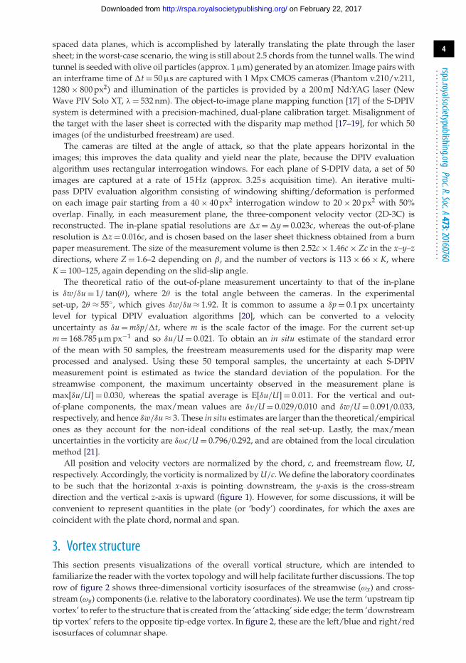
3. Vortex structureThis section presents visualizations of the overall vortical structure, which are intended tofamiliarize the reader with the vortex topology and will help facilitate further discussions. The toprow of figure 2 shows three-dimensional vorticity isosurfaces of the streamwise (ωx) and cross-stream (ωy) components (i.e. relative to the laboratory coordinates). We use the term ‘upstream tipvortex’ to refer to the structure that is created from the ‘attacking’ side edge; the term ‘downstreamtip vortex’ refers to the opposite tip-edge vortex. In figure 2, these are the left/blue and right/redisosurfaces of columnar shape.
on February 22, 2017http://rspa.royalsocietypublishing.org/Downloaded from
5
rspa.royalsocietypublishing.orgProc.R.Soc.A473:20160760
...................................................
−0.5 0 0.5
0.5
0
−0.5
y/c
x/c
x/c
z/c
0.5
0
−0.5
0.5
0
−0.5
0.5
0
−0.5
−0.5 0 0.5y/c
−0.5 0 0.5y/c
−0.5 0 0.5y/c
y/c y/c y/c y/c
y/c y/c y/c y/c
−0.5 0 0.5
1.5
1.0
0.5
0
−0.5
1.5
1.0
0.5
0
−0.5
1.5
1.0
0.5
0
−0.5
1.5
1.0
0.5
0
−0.5
−0.5 0 0.5 −0.5 0 0.5 −0.5 0 0.5
−0.5 0 0.5
−0.2−0.1
0
−0.2−0.1
0
−0.2−0.1
0
−0.2−0.1
0
(a)
−0.5 0 0.5
(b)
−0.5 0 0.5
(c)
−0.5 0 0.5
(d)
U
y
x
b = 0° b = 10° b = 20° b = 35°
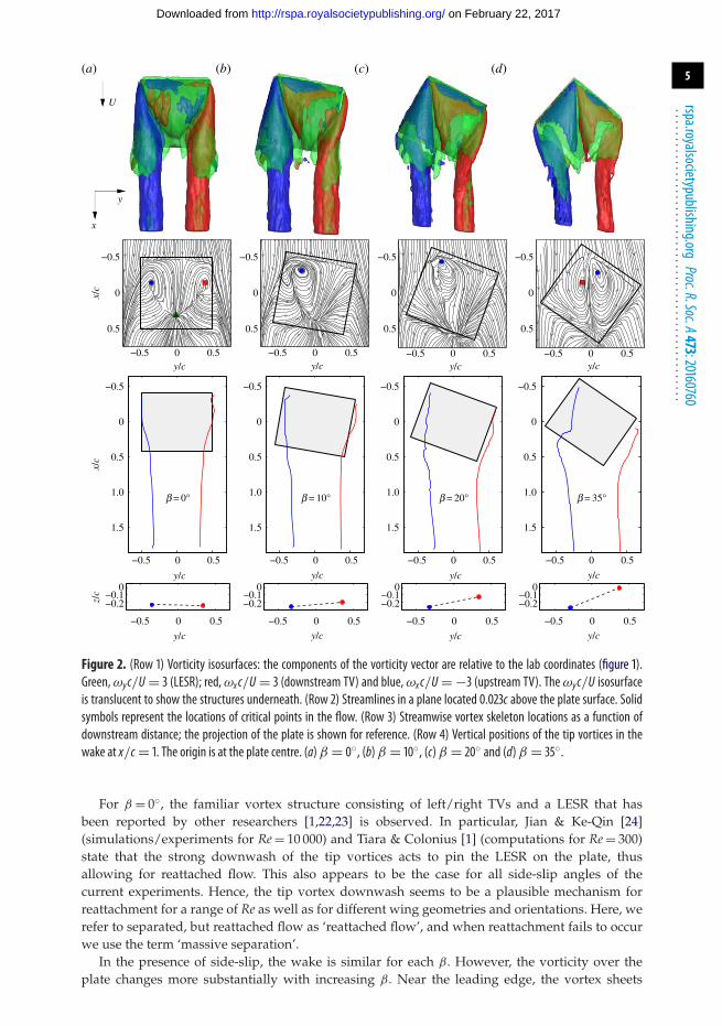
Figure 2. (Row 1) Vorticity isosurfaces: the components of the vorticity vector are relative to the lab coordinates (figure 1).Green,ωyc/U = 3 (LESR); red,ωx c/U = 3 (downstream TV) and blue,ωx c/U = −3 (upstream TV). Theωyc/U isosurfaceis translucent to show the structures underneath. (Row 2) Streamlines in a plane located 0.023c above the plate surface. Solidsymbols represent the locations of critical points in the flow. (Row 3) Streamwise vortex skeleton locations as a function ofdownstream distance; the projection of the plate is shown for reference. (Row 4) Vertical positions of the tip vortices in thewake at x/c = 1. The origin is at the plate centre. (a)β = 0◦, (b)β = 10◦, (c)β = 20◦ and (d)β = 35◦.
For β = 0◦, the familiar vortex structure consisting of left/right TVs and a LESR that hasbeen reported by other researchers [1,22,23] is observed. In particular, Jian & Ke-Qin [24](simulations/experiments for Re = 10 000) and Tiara & Colonius [1] (computations for Re = 300)state that the strong downwash of the tip vortices acts to pin the LESR on the plate, thusallowing for reattached flow. This also appears to be the case for all side-slip angles of thecurrent experiments. Hence, the tip vortex downwash seems to be a plausible mechanism forreattachment for a range of Re as well as for different wing geometries and orientations. Here, werefer to separated, but reattached flow as ‘reattached flow’, and when reattachment fails to occurwe use the term ‘massive separation’.
In the presence of side-slip, the wake is similar for each β. However, the vorticity over theplate changes more substantially with increasing β. Near the leading edge, the vortex sheets
on February 22, 2017http://rspa.royalsocietypublishing.org/Downloaded from
6
rspa.royalsocietypublishing.orgProc.R.Soc.A473:20160760
...................................................
from the upstream tip edge and the leading edge are comprised almost wholly of ωy vorticity(green isosurface). These shear layers appear to ‘blanket’ the vortical structure and so representa boundary-layer-like transition from the freestream velocity to the underlying vortex structures.The close proximity of the tip vortices results in a quick roll up of any trailing-edge vorticitybefore it can propagate far downstream. Because the tip vortices are formed along the wing tips,the near wake consists of columnar vortices that are already well into the roll-up process.
The second row of figure 2 plots streamlines in a plane located �x = 0.023c above the platesurface. For the β = 0◦ case, there is a streamline that makes a spatial distinction between the LESRand each TV. For β �= 0◦, the distinction between the LESR and downstream TV becomes moreambiguous. At zero side-slip, three stagnation/critical points can be identified. The two points onthe right and left are connected to a third point towards the trailing edge of the wing through twopositive bifurcation lines [25,26]. As the side-slip angle increases, the right and rear critical pointsdisappear from the wing resulting in the divergence and disappearance of the right bifurcationline, and by β = 35◦ another critical point on the left side of the wing appears and signifies alocally rotating flow opposite in sense to that associated with the original left critical point. Inessence, the left and right critical points of the zero side-slip case have switched positions, theflow along the z = 0 line is reversed. These changes in the streamline topology indicate how aflow control device could alter the flow to perform a roll manoeuvre.
It is desirable to represent the vortex structure in figure 2 in a more simplified manner, andin particular, we are primarily concerned with the TVs. We identify a ‘vortex skeleton’ given bythe position xv, and which is defined by vorticity-weighted centroids. The tip vortex locationsare calculated using the streamwise vorticity (i.e. ωx) in each x-plane of data to calculate thecorresponding (yv, zv) coordinates. To ‘track’ each vortex and distinguish from other, nearbystructures of the same sign vorticity, we use a clustering algorithm [27] that accumulates pointsin the vortex as determined by a thresholded vortex identification field. The circulation of thevortices is also computed in the process. Here, we are interested in the circulation generated byeach wing edge, whether it be in a rotating vortex or a shear layer. Therefore, we define the side-edge shear layers to be part of the tip vortex structures, and we opt to use a vorticity magnitudethreshold (rather than the Q-criterion, for example). The threshold value chosen was twice theuncertainty estimate in the vorticity, namely ωth = 2δω ≈ 1.2U/c. The calculation was repeatedwith different threshold values, and it was found that around the chosen value, the vortexlocations were not dramatically affected. The calculation does, however, have some difficulty nearthe leading edge where both the area of the tip vortices and their vorticity magnitudes are small.
The third row of figure 2 shows the cross-stream locations of the vortex skeleton (yv) as afunction of streamwise distance. These plots show a clearer distinction between the downstreamTV and the rolled up and tilted portion of the leading-edge shear layer. The downstream TVremains mostly parallel to its respective tip edge until β = 35◦ where it begins separating awayfrom the wing at the trailing edge. The upstream TV occupies more space over the wing as theside-slip is increased, but also remains nominally parallel to its edge. At β = 35◦, the upstreamTV and the tilted, rolled-up portion of the leading-edge shear layer resemble the well-knownleading-edge vortices of (non-slender) delta wings [28]. After a short distance into the wake, thecross-stream locations of both tip vortices remain essentially straight.
The fourth row of figure 2 plots the vertical vortex locations (zv) at the plane x/c = 1 in thewake. This shows that with increasing side-slip the downstream TV is shed at a higher locationinto the wake, whereas the upstream TV positions are almost the same. As such, the wakevortex structure becomes more tilted, which indicates a total torque in the vortex structure thatrepresents some contribution to the rolling moment on the wing.
4. Vortex modelIn this section, we aim to develop a simple vortex model to predict aerodynamic loads andmoments, with the angle of attack, side-slip angle and aspect ratio as variables. There aremany successful aerodynamic models and relations for finite wings that already exist, such as
on February 22, 2017http://rspa.royalsocietypublishing.org/Downloaded from
7
rspa.royalsocietypublishing.orgProc.R.Soc.A473:20160760
...................................................
the collected works of Prandtl et al. [29], Bollay [30], Falkner [31], Jones [32], Helmbold [33],Kuchemann [34], Brown & Michael [35], Mangler & Smith [36], Polhmaus [16], Lamar [37] andseveral extensions of these models. Some models are based on slender body theory, but severalothers employ lifting surface methods (e.g. Multhopp [38]) with three-dimensional spanwise andchordwise loadings. Some of the simpler existing models that rely on slender body theory usuallyhave an elliptical spanwise lift distribution. For example, the pointed slender wing model of Jones[32] assumes a two-dimensional cross-plane flow at each chord position, and it is shown that thisflow is characterized by an elliptical loading distribution across the local span. In this way, thatmodel is limited to low angles of attack (as well as aspect ratios of course). More involved modelsuse expansions to improve the range of applicability of the model, as well as to include relationsfor vortex positions and strengths. The leading-edge suction analogy of Polhamus, which wasextended by Lamar, provides a nonlinear relation between forces and the angle of attack that hasbeen shown to be accurate at high incidences. However, as pointed out by Riley & Smith [39],the Polhamus method does not offer insight on the actual separated flow structures; in turn, theydeveloped a model that incorporates these features and yields results comparable to a slenderbody theory [40].
Given the vast amount of previous work, we do not intend to build up to these models, butrather to use their common features and results as inspiration to an oversimplified representationof the wing and vortex structure that bypasses some of the flow details addressed in the moresophisticated approaches. The novelty of our proposed model is to adopt the nonlinear vortexsuction relation with the angle of attack of the Polhamus method and to represent the separatedflow structures by line vortices with prescribed circulation distributions that are characteristicof large angles of attack, thus extending the range of applicability while circumventing thespecification of more detailed information of the flow features. As such, a lifting surfacecalculation is not needed nor used. To make the model as simple as possible, the number offree parameters is kept to a minimum. The circulation distributions are determined from a newinterpretation of a limiting slender-body-based potential flow model developed next in §4a andother assumptions about the vortex system are supported by the experimental findings of theprevious sections.
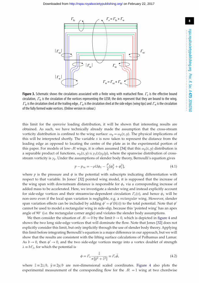
In classical lifting line theory, the flow is potential in the sense that it remains attached to thewing. Hence, the circulation around the wing is equal to the circulation of the tip vortices asa consequence of the Helmholtz law of persistence of irrotationality. For wings with separatedbut reattached flow there is an additional circulation distribution associated with the separationregion. However, the vortex lines that represent this leading-edge separation region begin andend on the wing and thus have an ‘image’ inside the wing that satisfies the Helmholtz law.Furthermore, they can be considered as bound vortices, because the LESR moves with the wing.Consider a wing that has established a reattached flow as illustrated in figure 3. The circulationrepresenting the LESR is Γle and that of the tip vortices in the wake after the roll-up processis Γw. The total or effective bound circulation (owing to reattachment) is Γo and is related byΓo = Γle + Γw. Note that Γle cannot be determined independently, say by experiment, but maybe found by knowledge of Γo and Γw, both of which can be measured. The circulation of theside-edge vortices Γse forms along the wing tip edges, and rolls up the vorticity, with circulationΓte, shed from the trailing edge. After the roll-up process completes, the circulation of the waketip vortices is Γw = Γse + Γte. Next, we begin with determining the different loading/circulationdistributions. The model also requires determination of the downwash on the vortex system,and will be found subsequent to the circulation. The results are then substituted into equationsof the Polhamus method and the remaining parameters are determined by matching limitingbehaviours with α andA to those predicted by existing, well-established models.
(a) Spanwise loadingIn general, the cross-stream vorticity distribution is three-dimensional. Here we address thespanwise loading by appealing to slender body theory. Although it may seem strange to consider
on February 22, 2017http://rspa.royalsocietypublishing.org/Downloaded from
8
rspa.royalsocietypublishing.orgProc.R.Soc.A473:20160760
...................................................
Gw = Gse + Gte
Go = Gle + Gw
ÔGteÔ
ÔGwÔ
ÔGseÔ
Gle
Gte
Gse
Figure 3. Schematic shows the circulations associated with a finite wing with reattached flow. Γo is the effective boundcirculation, Γle is the circulation of the vortices representing the LESR; the dots represent that they are bound to the wing.Γte is the circulation shed at the trailing edge,Γse is the circulation shed at the side edges (wing tips) andΓw is the circulationof the fully formed wake vortices. (Online version in colour.)
this limit for the spanwise loading distribution, it will be shown that interesting results areobtained. As such, we have technically already made the assumption that the cross-streamvorticity distribution is confined to the wing surface: ωy = ωy(x, y). The physical implications ofthis will be interpreted shortly. The variable x is now taken to represent the distance from theleading edge as opposed to locating the centre of the plate as in the experimental portion ofthis paper. For models of low-A wings, it is often assumed [34] that this ωy(x, y) distribution isa separable product of functions, ωy(x, y) ∝ γx(x)γy(y), where the spanwise distribution of cross-stream vorticity is γy. Under the assumptions of slender body theory, Bernoulli’s equation gives
p − p∞ = −ρUφx − ρ
2[φ2
y + φ2z ], (4.1)
where p is the pressure and φ is the potential with subscripts indicating differentiation withrespect to that variable. In Jones’ [32] pointed wing model, it is supposed that the increase ofthe wing span with downstream distance is responsible for φx via a corresponding increase ofadded mass to be accelerated. Here, we investigate a slender wing and instead explicitly accountfor side-edge vortices and their streamwise-dependent circulation Γx(x), and hence φx will benon-zero even if the local span variation is negligible, e.g. a rectangular wing. However, slenderspan variation effects can be included by adding φ′ = φ′(b(x)) to the total potential. Note that φ′cannot be used to model a rectangular wing in side-slip, because this ‘pointed wing’ has an apexangle of 90◦ (i.e. the rectangular corner angle) and violates the slender body assumptions.
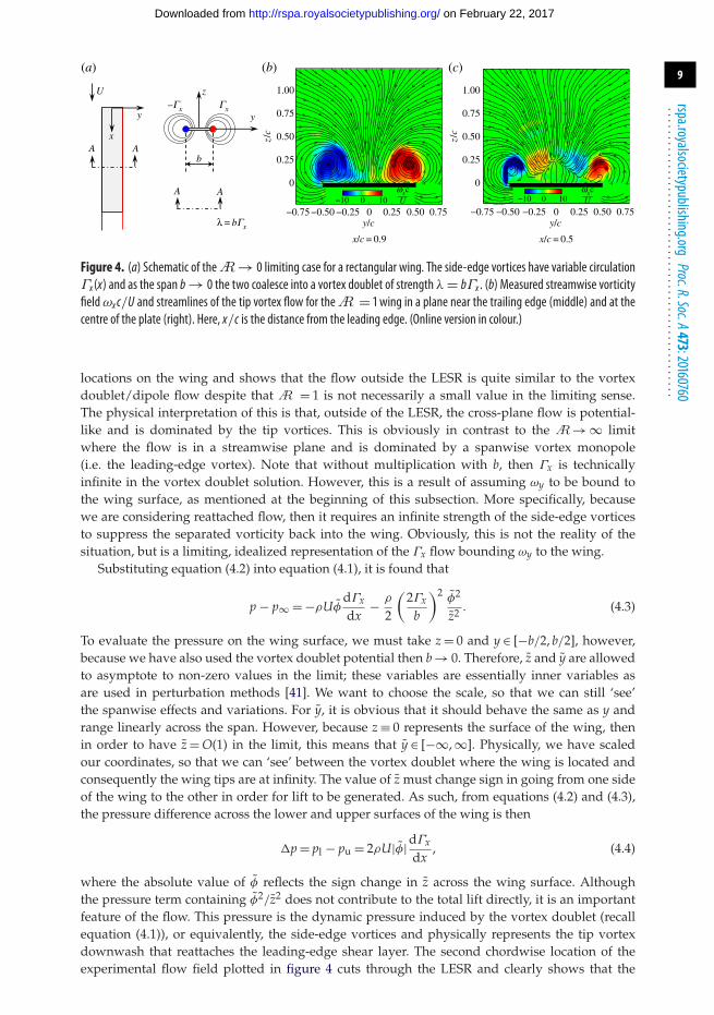
We then consider the situation ofA→ 0 by the limit b → 0, which is depicted in figure 4 andshows the two long side-edge vortices that will dominate the flow. Note that Jones [32] does notexplicitly consider this limit, but only implicitly through the use of slender body theory. Applyingthis limit before integrating Bernoulli’s equation is a major difference in our approach, but we willshow that the results are consistent with the lifting surface calculations of Polhamus and Lamar.As b → 0, then φ′ → 0, and the two side-edge vortices merge into a vortex doublet of strengthλ ≡ bΓx, for which the potential is
φ = Γxz
π [y2 + z2]≡ Γxφ, (4.2)
where z ≡ 2z/b, y ≡ 2y/b are non-dimensional scaled coordinates. Figure 4 also plots theexperimental measurement of the corresponding flow for the A = 1 wing at two chordwise
on February 22, 2017http://rspa.royalsocietypublishing.org/Downloaded from
9
rspa.royalsocietypublishing.orgProc.R.Soc.A473:20160760
...................................................
U
y y
z
xAA
A A
l = bGx
–Gx Gx
b
y/c
z/c
z/c
−0.75−0.50 −0.25 0 0.25 0.50 0.75
0
0.25
0.50
0.75
1.00
(a) (b) (c)
0
0.25
0.50
0.75
1.00
−10 0 10wxc
x/c = 0.9 x/c = 0.5
y/c−0.75 −0.50 −0.25 0 0.25 0.50 0.75
−10 0 10UwxcU
Figure 4. (a) Schematic of theA→ 0 limiting case for a rectangular wing. The side-edge vortices have variable circulationΓx (x) and as the span b→ 0 the two coalesce into a vortex doublet of strengthλ = bΓx . (b) Measured streamwise vorticityfieldωx c/U and streamlines of the tip vortex flow for theA = 1 wing in a plane near the trailing edge (middle) and at thecentre of the plate (right). Here, x/c is the distance from the leading edge. (Online version in colour.)
locations on the wing and shows that the flow outside the LESR is quite similar to the vortexdoublet/dipole flow despite that A = 1 is not necessarily a small value in the limiting sense.The physical interpretation of this is that, outside of the LESR, the cross-plane flow is potential-like and is dominated by the tip vortices. This is obviously in contrast to the A→ ∞ limitwhere the flow is in a streamwise plane and is dominated by a spanwise vortex monopole(i.e. the leading-edge vortex). Note that without multiplication with b, then Γx is technicallyinfinite in the vortex doublet solution. However, this is a result of assuming ωy to be bound tothe wing surface, as mentioned at the beginning of this subsection. More specifically, becausewe are considering reattached flow, then it requires an infinite strength of the side-edge vorticesto suppress the separated vorticity back into the wing. Obviously, this is not the reality of thesituation, but is a limiting, idealized representation of the Γx flow bounding ωy to the wing.
Substituting equation (4.2) into equation (4.1), it is found that
p − p∞ = −ρUφdΓx
dx− ρ
2
(2Γx
b
)2φ2
z2 . (4.3)
To evaluate the pressure on the wing surface, we must take z = 0 and y ∈ [−b/2, b/2], however,because we have also used the vortex doublet potential then b → 0. Therefore, z and y are allowedto asymptote to non-zero values in the limit; these variables are essentially inner variables asare used in perturbation methods [41]. We want to choose the scale, so that we can still ‘see’the spanwise effects and variations. For y, it is obvious that it should behave the same as y andrange linearly across the span. However, because z ≡ 0 represents the surface of the wing, thenin order to have z = O(1) in the limit, this means that y ∈ [−∞, ∞]. Physically, we have scaledour coordinates, so that we can ‘see’ between the vortex doublet where the wing is located andconsequently the wing tips are at infinity. The value of z must change sign in going from one sideof the wing to the other in order for lift to be generated. As such, from equations (4.2) and (4.3),the pressure difference across the lower and upper surfaces of the wing is then
�p = pl − pu = 2ρU|φ|dΓx
dx, (4.4)
where the absolute value of φ reflects the sign change in z across the wing surface. Althoughthe pressure term containing φ2/z2 does not contribute to the total lift directly, it is an importantfeature of the flow. This pressure is the dynamic pressure induced by the vortex doublet (recallequation (4.1)), or equivalently, the side-edge vortices and physically represents the tip vortexdownwash that reattaches the leading-edge shear layer. The second chordwise location of theexperimental flow field plotted in figure 4 cuts through the LESR and clearly shows that the
on February 22, 2017http://rspa.royalsocietypublishing.org/Downloaded from
10
rspa.royalsocietypublishing.orgProc.R.Soc.A473:20160760
...................................................
potential flow outside the LESR acts to promote reattachment. Hence, this analytical expressioncould be employed to predict lift stall.
Returning to �p, we can integrate along the chord, which assuming the side-edges vortices tohave zero circulation at the leading edge, then gives the spanwise loading distribution:∫
�p dx = 2ρU|φ|Γse, (4.5)
where Γse = Γx(x = c) is the fully developed circulation of the side-edge vortex. Much in the waythat Jones’ result for the spanwise lift distribution is independent of planform, the above result isindependent of Γx(x). Also, note that while the chord c should be large enough for equation (4.1)to apply, we have not taken c → ∞ to makeA→ 0.
Because we are assuming reattached flow, the dependence of the forces on angle of attack isrepresented by the trigonometric terms in the Polhamus method (see equation (4.17) in §4e). Inother words, the integration of the spanwise loading distribution in equation (4.5) would give thelift-curve slope, say Lα , in the case ofA→ 0; the result of this is
Lα =∫
2ρUφΓse dy = ρUbΓse
∫ ∞
−∞φ dy = ρUbΓse, (4.6)
and it should be noted that this is independent of the value of |z|, because the limits on the integralare from positive to negative infinity and z is finite. Now, consider a rectangular wing and adelta wing whose maximum spans and root chord lengths are equal, so that the rectangle of areaS = bc is the bounding box on the delta wing of area S� = bc/2. This best isolates the sweep angleeffects by creating an equal competition between the planform area and aspect ratio (A= b/cversusA� = 2b/c). Nonetheless, the above result should be consistent with that of Jones, whichis CLα
= (π/2)A� = πA. The meaning of this is that, while Jones’ lift-curve slope is valid for allslender wings, including delta and rectangular wings, it is so for different numerical ranges ofA. For rectangular wings the value ofA must be comparably smaller, because the assumptionof slenderness is violated otherwise; this effect of wing geometry is a fundamental differencebetween delta and rectangular wings. For example, an A� = 1 delta wing has a sweep angleof Λ ≈ 76◦ and is therefore slender. However, an A = 1 rectangular wing is not necessarilyslender and because A= b/c this obviously represents the middle ground of when spanwiseand chordwise dimensions are equally important. Therefore, the range of numerical values ofAfor which Jones’ result is valid for rectangular wings is then half that of a comparable delta wing.
Non-dimensionalizing equation (4.6) and equating it to the result that CL,α = πA gives
ρUbΓse
(1/2)ρU2S= 2Γse
Uc= 2Γse
UbA= πA → 2Γse
Ub= π . (4.7)
In §4e, where we apply the Polhamus method, it will be seen that the right-most term inequation (4.7) is equivalent to the coefficient of the vortex force constituent (i.e. Kv,se) asA→ 0.Furthermore, the right-hand side, namely π , is exactly the value computed by Polhamus [16] via alifting surface method for delta wings asA→ 0. The same value was computed by Lamar [37] forrectangular wings with a modified method and using impulsive chordwise loading and ellipticalspan loading. Lamar explained that the reason the two limiting values are the same is because theleading edges of the delta wing become like the side edges of a rectangular wing asA→ 0. Thus,our model is an interpretation of the Jones slender wing model for rectangular wings and whichanalytically predicts the correct behaviour in the zero-aspect-ratio limit.
Lastly, we revert back to the spanwise loading distribution, which is proportional to thespanwise circulation distribution, γy, which, in turn, is proportional to φ. In order to find whatform this distribution takes, we need to find a value for z and one that has physical meaning.The expression for the spanwise velocity v = φy shows that in order for this component to bephysically consistent with a flow going around the tip from the lower to upper side then z < 0;note the exclusion of z = 0, which returns the degenerate case of a singular pressure at theorigin. Although each velocity is finite, continuous and differentiable, we now satisfy a Kutta-like
on February 22, 2017http://rspa.royalsocietypublishing.org/Downloaded from
11
rspa.royalsocietypublishing.orgProc.R.Soc.A473:20160760
...................................................
−0.75 −0.50 −0.25 0 0.25 0.50 0.750
0.5
1.0
1.5
2.0
y/c
cros
s-st
ream
cir
cula
tion
G y/U
c
para. dist.
(a)
0 0.5 1.0 1.5 2.0
−1.0
−0.5
0
0.5
1.0
distance from LE corner: (x – xle)/c
TV
cir
cula
tions
: Gx/U
c
upstream TV
LE shear layerroll-up and tilt
downstream TV
(b)
b = 0°b = 10°b = 20°b = 35°
lin. dist.
b = 0°b = 10°b = 20°b = 35°
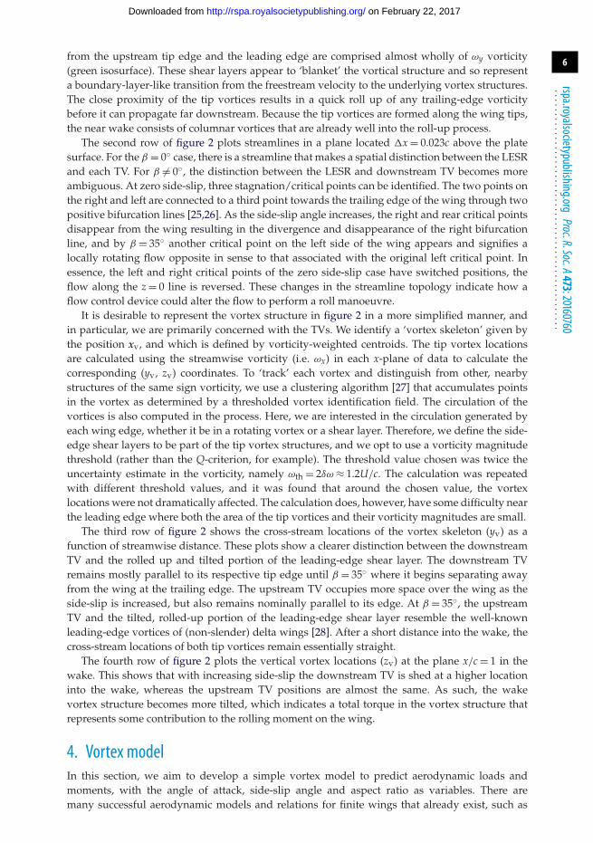
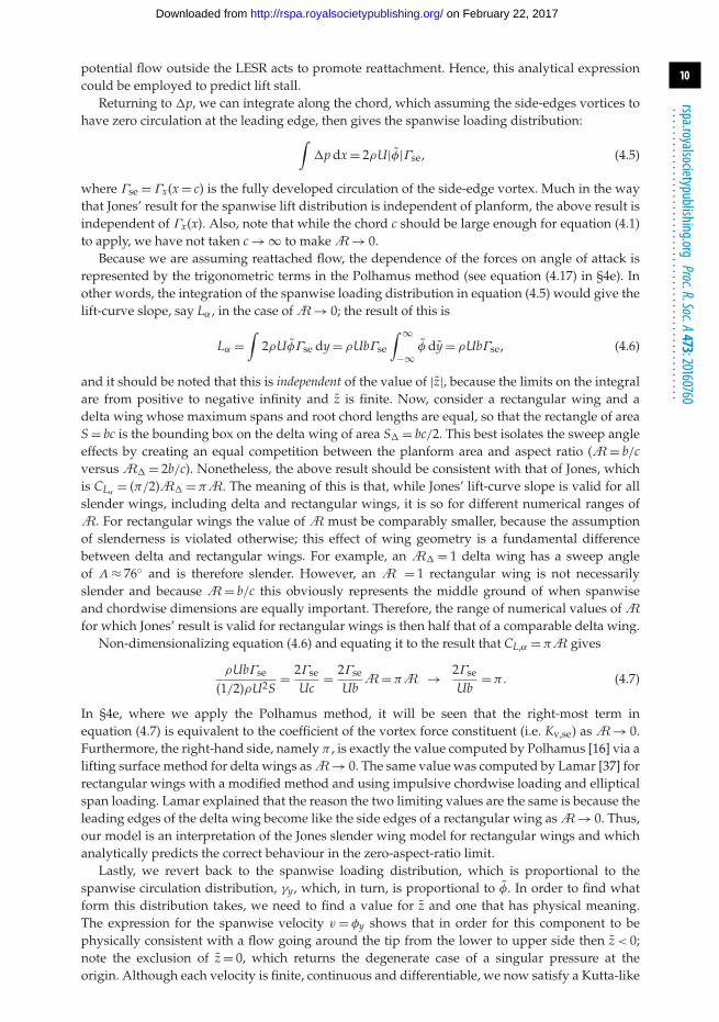
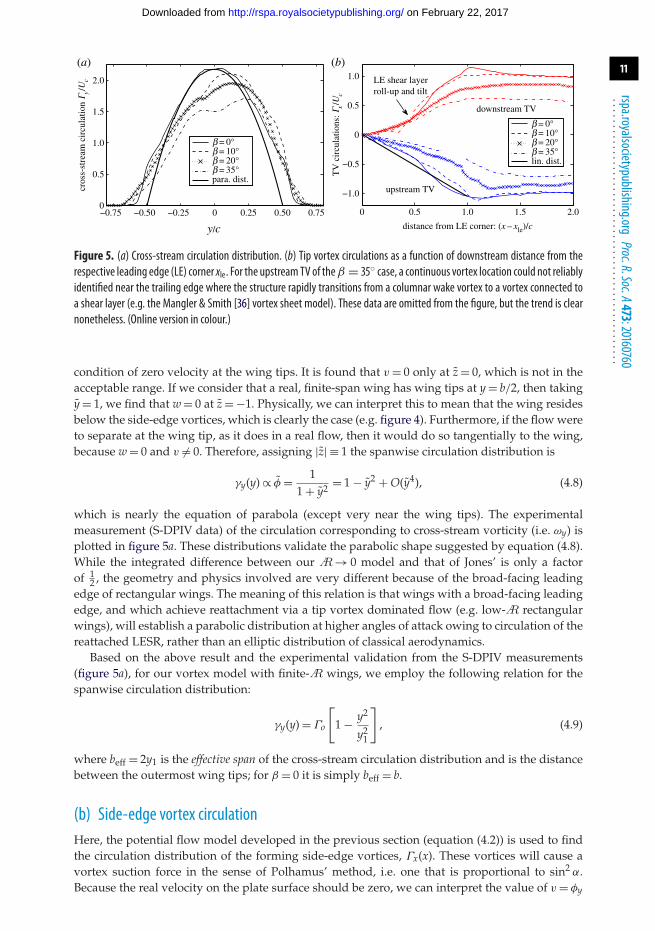
Figure 5. (a) Cross-stream circulation distribution. (b) Tip vortex circulations as a function of downstream distance from therespective leading edge (LE) corner xle. For the upstream TV of theβ = 35◦ case, a continuous vortex location could not reliablyidentified near the trailing edge where the structure rapidly transitions from a columnar wake vortex to a vortex connected toa shear layer (e.g. the Mangler & Smith [36] vortex sheet model). These data are omitted from the figure, but the trend is clearnonetheless. (Online version in colour.)
condition of zero velocity at the wing tips. It is found that v = 0 only at z = 0, which is not in theacceptable range. If we consider that a real, finite-span wing has wing tips at y = b/2, then takingy = 1, we find that w = 0 at z = −1. Physically, we can interpret this to mean that the wing residesbelow the side-edge vortices, which is clearly the case (e.g. figure 4). Furthermore, if the flow wereto separate at the wing tip, as it does in a real flow, then it would do so tangentially to the wing,because w = 0 and v �= 0. Therefore, assigning |z| ≡ 1 the spanwise circulation distribution is
γy(y) ∝ φ = 11 + y2 = 1 − y2 + O(y4), (4.8)
which is nearly the equation of parabola (except very near the wing tips). The experimentalmeasurement (S-DPIV data) of the circulation corresponding to cross-stream vorticity (i.e. ωy) isplotted in figure 5a. These distributions validate the parabolic shape suggested by equation (4.8).While the integrated difference between our A→ 0 model and that of Jones’ is only a factorof 1
2 , the geometry and physics involved are very different because of the broad-facing leadingedge of rectangular wings. The meaning of this relation is that wings with a broad-facing leadingedge, and which achieve reattachment via a tip vortex dominated flow (e.g. low-A rectangularwings), will establish a parabolic distribution at higher angles of attack owing to circulation of thereattached LESR, rather than an elliptic distribution of classical aerodynamics.
Based on the above result and the experimental validation from the S-DPIV measurements(figure 5a), for our vortex model with finite-A wings, we employ the following relation for thespanwise circulation distribution:
γy(y) = Γo
[1 − y2
y21
], (4.9)
where beff = 2y1 is the effective span of the cross-stream circulation distribution and is the distancebetween the outermost wing tips; for β = 0 it is simply beff = b.
(b) Side-edge vortex circulationHere, the potential flow model developed in the previous section (equation (4.2)) is used to findthe circulation distribution of the forming side-edge vortices, Γx(x). These vortices will cause avortex suction force in the sense of Polhamus’ method, i.e. one that is proportional to sin2 α.Because the real velocity on the plate surface should be zero, we can interpret the value of v = φy
on February 22, 2017http://rspa.royalsocietypublishing.org/Downloaded from
12
rspa.royalsocietypublishing.orgProc.R.Soc.A473:20160760
...................................................
near the wing tip to be the strength of a shed vortex sheet that generates the side-edge vortex
v = dΓx
dx= Γx
2φy
b, (4.10)
with the second equality coming from equation (4.2). The exponential solution of this first-orderdifferential equation cannot satisfy the condition that Γx(0) = 0. This is not surprising, because thislocation is the corner of the wing where the two-dimensional assumption of slender body theoryis invalid. However, if we assume that this represents the tip vortex growth rate downstream ofthe leading edge, then after expanding the exponential we obtain
dΓx
dx∼ 2φy
b+ O(x), (4.11)
and indicates a constant growth rate or a linear growth of Γx ∼ x. This near linear growth is alsothe trend obtained by some of the simpler slender body wing models [39,40]. Hence, for ourmodel, we now assume that each side-edge vortex has
Γx(x) = Γsexc
, (4.12)
where x is the distance from the respective leading-edge corner along the chord for the case ofside-slip. This expression is further supported by our experimental measurements of the side-edge vortex circulations, which are shown in figure 5b. Moreover, figure 5 shows that thecirculation magnitudes maintain a nominally constant value in the wake, and that these valuesare the same for each TV. With increasing side-slip the circulation values decrease, which is thesame trend for the LEVs of a delta wing as the sweep angle is increased [42]. Closer observationof the experimental circulations shows that the downstream TV experiences two different growthrates. From the leading edge the first growth rate is slower, when compared with the upstreamTV. However, at around the mid-chord location, the rolled-up and tilted portion of the leading-edge shear layer begins to feed into the downstream TV and constitutes the second growth ratephase, which is comparable to the rate of the upstream TV. However, the circulation differencesare minor, and we ignore this effect in our model.
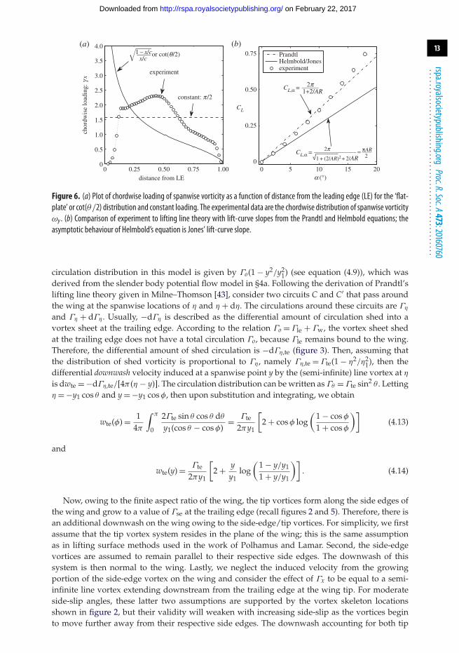
(c) Chordwise loadingFor low-A wings whose aspect ratios are of order unity, the total chordwise loading willobviously depend on the distribution of cross-stream vorticity, ωy(x, y) = γx(x)γy(y), and not justthe circulation of the side-edge vortices, Γx(x), of the previous section. It is often assumedthat γx(x) is impulsive, constant or has the ‘flat-plate’ distribution [34] also called the ‘cot(θ/2)’distribution [37], which is given by γx ∼ √
(1 − x/c)/(x/c). When integrated over the chord thisgives a resultant force proportional to π/2 that acts at the quarter-point from the leading edge.In a real flow, obviously, the loading will not be impulsive. Figure 6a shows the ‘flat-plate’and constant loadings along with the chordwise distribution of the experimental cross-streamvorticity averaged over the span of theA = 1 plate. Near the leading edge the experimental γx
shows a rapid increase to a somewhat constant value and then decreases in a fashion similar tothe flat plate distribution. Therefore, it appears the experimental data have features of both the‘flat-plate’ and constant loading types and we now assume that the chordwise loading in ourmodel is a combination of the two. As a result, the integrated effect of this distribution is still aforce proportional to π/2, but which acts somewhere between the quarter-chord and mid-chordpoints, because the constant loading acts at the mid-chord. Therefore, ωy = (π/2)γy(y), where theπ/2 factor will later be absorbed into γy for convenience.
(d) DownwashIn the Polhamus method, the vortex forces are affected by the downwash on the vortex system,which we now compute using the specified the circulation distributions. Recall that the spanwise
on February 22, 2017http://rspa.royalsocietypublishing.org/Downloaded from
13
rspa.royalsocietypublishing.orgProc.R.Soc.A473:20160760
...................................................
0 0.25 0.50 0.75 1.000
0.5
1.0
1.5
2.0
2.5
3.0
3.5
4.0
distance from LE
chor
dwis
e lo
adin
g: g
x
constant: p/2
experiment
1 – x/cx/c
or cot(q/2)
(a)
0 5 10 15 200
0.25
0.50
0.75
a (°)
CL
PrandtlHelmbold/Jonesexperiment
2p ª1 + (2/AR)2 + 2/AR
pAR2
(b)
CL,a =
CL,a =
1+2/AR2p
Figure 6. (a) Plot of chordwise loading of spanwise vorticity as a function of distance from the leading edge (LE) for the ‘flat-plate’ or cot(θ/2) distribution and constant loading. The experimental data are the chordwise distribution of spanwise vorticityωy . (b) Comparison of experiment to lifting line theory with lift-curve slopes from the Prandtl and Helmbold equations; theasymptotic behaviour of Helmbold’s equation is Jones’ lift-curve slope.
circulation distribution in this model is given by Γo(1 − y2/y21) (see equation (4.9)), which was
derived from the slender body potential flow model in §4a. Following the derivation of Prandtl’slifting line theory given in Milne–Thomson [43], consider two circuits C and C′ that pass aroundthe wing at the spanwise locations of η and η + dη. The circulations around these circuits are Γη
and Γη + dΓη. Usually, −dΓη is described as the differential amount of circulation shed into avortex sheet at the trailing edge. According to the relation Γo = Γle + Γw, the vortex sheet shedat the trailing edge does not have a total circulation Γo, because Γle remains bound to the wing.Therefore, the differential amount of shed circulation is −dΓη,te (figure 3). Then, assuming thatthe distribution of shed vorticity is proportional to Γη, namely Γη,te = Γte(1 − η2/η2
1), then thedifferential downwash velocity induced at a spanwise point y by the (semi-infinite) line vortex at η
is dwte = −dΓη,te/[4π (η − y)]. The circulation distribution can be written as Γθ = Γte sin2 θ . Lettingη = −y1 cos θ and y = −y1 cos φ, then upon substitution and integrating, we obtain
wte(φ) = 14π
∫ π
0
2Γte sin θ cos θ dθ
y1(cos θ − cos φ)= Γte
2πy1
[2 + cos φ log
(1 − cos φ
1 + cos φ
)](4.13)
and
wte(y) = Γte
2πy1
[2 + y
y1log
(1 − y/y1
1 + y/y1
)]. (4.14)
Now, owing to the finite aspect ratio of the wing, the tip vortices form along the side edges ofthe wing and grow to a value of Γse at the trailing edge (recall figures 2 and 5). Therefore, there isan additional downwash on the wing owing to the side-edge/tip vortices. For simplicity, we firstassume that the tip vortex system resides in the plane of the wing; this is the same assumptionas in lifting surface methods used in the work of Polhamus and Lamar. Second, the side-edgevortices are assumed to remain parallel to their respective side edges. The downwash of thissystem is then normal to the wing. Lastly, we neglect the induced velocity from the growingportion of the side-edge vortex on the wing and consider the effect of Γx to be equal to a semi-infinite line vortex extending downstream from the trailing edge at the wing tip. For moderateside-slip angles, these latter two assumptions are supported by the vortex skeleton locationsshown in figure 2, but their validity will weaken with increasing side-slip as the vortices beginto move further away from their respective side edges. The downwash accounting for both tip
on February 22, 2017http://rspa.royalsocietypublishing.org/Downloaded from
14
rspa.royalsocietypublishing.orgProc.R.Soc.A473:20160760
...................................................
vortices is then simply
wse(y) = Γse
2π
[1
y1 + y+ 1
y1 − y
]= Γse
2πy1
[1
1 − y2/y21
]= ΓseΓo
2πy1
[1
γy(y)
]. (4.15)
Equation (4.15) is interesting insofar as the side-edge vortex-induced velocity (i.e. between twosemi-infinite line vortices) is not directly dependent on our particular choice of γy as a parabola.However, the limit of these two vortices approaching each other is the vortex doublet, which wasused in deriving the spanwise circulation distribution. Clearly, this downwash is not constantalong the span as it is for Prandtl’s lifting line theory, but rather it will result in a constant vortexforce distribution along the span, because this force is proportional to wseγy.
Obviously, the downwash velocities are each singular at the wing tips and at a small distanceξ = |y1 − y| from the wing tip, we have
wse + wte ∼ Γse
4πξ− Γte
2πy1log
[ξ
y1
]. (4.16)
Therefore, the velocity at the trailing-edge corners can be non-singular, namely zero, only if Γte isinfinitely larger than Γse. That this condition cannot be satisfied seems unavoidable, because whenthe trailing-edge vorticity rolls up into the side-edge vortices the total wake vortex circulation, Γw
(figure 3), will be Γw = Γse + Γte and it is clear that for low-Awings that Γse obtains a significantportion of Γw by the trailing edge. In other words, if A is sufficiently low, then the side-edgevortices quickly roll up any vorticity shed from the trailing edge meaning that Γse ≈ Γw, and thenear wake consists of the well-formed columnar tip vortices; this feature is observed in the currentexperiments (recall figures 2 and 5b). Nevertheless, we content ourselves with the singularity byrecalling that the circulation γy is zero at the wing tips and thus the associated induced force willbe finite.
(e) Potential and vortex forcesHere, we employ the method of Polhamus [16] to determine the potential and vortex suctionforces that act normal to the wing surface. We assume the reader is familiar with the concept of thismethod and refer those that are not to the original paper. The force coefficients are normalized by1/2ρU2S, where S is the planform area, which is S = bc for the rectangular wings. The expressionsfor the force coefficients are
CN = Kp sin α cos α + Kv sin2 α → CL = CN cos α, CD = CN sin α. (4.17)
The coefficients Kp and Kv represent the potential and vortex constituents. The potential force isobtained from integration of γy = (π/2)Γo(1 − y2/y2
1) across the effective span beff = 2y1, where theπ/2 factor represents the integrated effect of the chordwise loading (see §4c). The result is
Kp = 2π
3Γo
Ucbeff
b. (4.18)
Next, following Lamar, we write Kv = Kv,le + Kv,se, where the first term represents the vortexsuction force associated with the leading-edge circulation, and the second term represents theside-edge vortex force. The leading-edge vortex force is affected by the downwash of thewake vortex system (trailing-edge vorticity and side-edge/tip vortex), namely wte + wse. Againintegrating across the effective span gives
Kv,le = Kp
[1 − 3
2πA
bbeff
(Γte + Γse
Uc
)]= Kp
[1 − 3
2π
Γw
Ubeff
]. (4.19)
where the second equality comes from the relation Γte + Γse = Γw (recall figure 3a).The side-edge vortex force is obtained by integrating Γx along the chord. We assume that
the side-edge vortices do not experience a downwash from the cross-stream circulation. Thereasoning behind this is that the downwash of the tip vortex system is largely responsible forthe reattached flow and thus the latter would not exist without the former. We considered a
on February 22, 2017http://rspa.royalsocietypublishing.org/Downloaded from
15
rspa.royalsocietypublishing.orgProc.R.Soc.A473:20160760
...................................................
max. span:no TV lift aft
upstream TVeffective length: c
downstream TVeffective length: x1
U
xs
bsys
xp
yp
−40 −20 0 20 40−0.4
−0.3
−0.2
−0.1
0
0.1
0.2
0.3
0.4
a (°)
pitc
hing
mom
ent:
Cm
modelexperiment
b = 0
(b)(a)
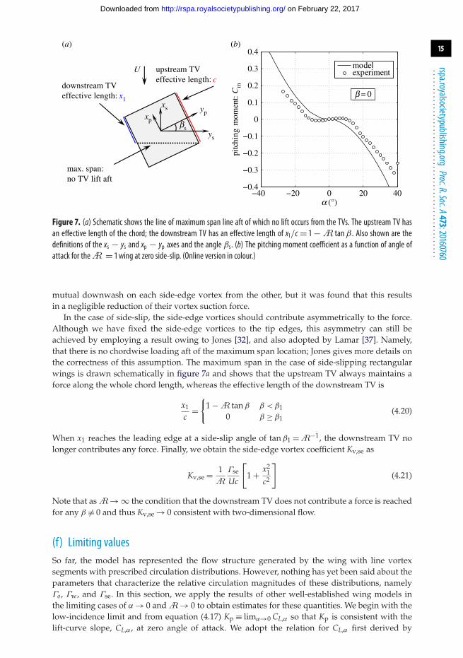
Figure 7. (a) Schematic shows the line of maximum span line aft of which no lift occurs from the TVs. The upstream TV hasan effective length of the chord; the downstream TV has an effective length of x1/c = 1 −A tanβ . Also shown are thedefinitions of the xs − ys and xp − yp axes and the angle βs. (b) The pitching moment coefficient as a function of angle ofattack for theA = 1 wing at zero side-slip. (Online version in colour.)
mutual downwash on each side-edge vortex from the other, but it was found that this resultsin a negligible reduction of their vortex suction force.
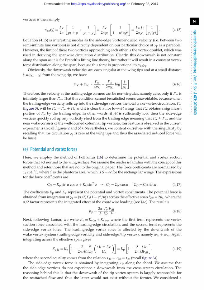
In the case of side-slip, the side-edge vortices should contribute asymmetrically to the force.Although we have fixed the side-edge vortices to the tip edges, this asymmetry can still beachieved by employing a result owing to Jones [32], and also adopted by Lamar [37]. Namely,that there is no chordwise loading aft of the maximum span location; Jones gives more details onthe correctness of this assumption. The maximum span in the case of side-slipping rectangularwings is drawn schematically in figure 7a and shows that the upstream TV always maintains aforce along the whole chord length, whereas the effective length of the downstream TV is
x1
c=
{1 −A tan β β < β1
0 β ≥ β1(4.20)
When x1 reaches the leading edge at a side-slip angle of tan β1 =A−1, the downstream TV nolonger contributes any force. Finally, we obtain the side-edge vortex coefficient Kv,se as
Kv,se = 1A
Γse
Uc
[1 + x2
1c2
](4.21)
Note that asA→ ∞ the condition that the downstream TV does not contribute a force is reachedfor any β �= 0 and thus Kv,se → 0 consistent with two-dimensional flow.
(f) Limiting valuesSo far, the model has represented the flow structure generated by the wing with line vortexsegments with prescribed circulation distributions. However, nothing has yet been said about theparameters that characterize the relative circulation magnitudes of these distributions, namelyΓo, Γw, and Γse. In this section, we apply the results of other well-established wing models inthe limiting cases of α → 0 andA→ 0 to obtain estimates for these quantities. We begin with thelow-incidence limit and from equation (4.17) Kp ≡ limα→0 CL,α so that Kp is consistent with thelift-curve slope, CL,α , at zero angle of attack. We adopt the relation for CL,α first derived by
on February 22, 2017http://rspa.royalsocietypublishing.org/Downloaded from
16
rspa.royalsocietypublishing.orgProc.R.Soc.A473:20160760
...................................................
Helmbold [33], which is known to be accurate for low-A unswept or straight wings:
Kp = 2πA√A2 + 4 + 2
. (4.22)
From equation (4.18), we can now obtain a relation for Γo in terms of Kp. As an aside, if onelinearizes the Prandtl lifting line (CL = 2πAα/(2 +A)) with respect toA it is found that CL =πAα. As a result one will find that, while this does not accurately capture the lift-curve slope atzero angle of attack, it does better predict the lift coefficient for a larger angle of attack range forrectangular wings than does Jones’ results (figure 6b).
Now, moving on to the zero-aspect-ratio limit, we note that Kp, Kv,le → 0 and the onlyremaining term is the side-edge vortex force term. First, we define Γse ≡ kseΓo and use the limitingvalue of Kv,se to obtain kse. This is done by matching the force coefficient to a slender body modelconsistent with the prescribed loading, which recalling from §4a it was shown that Kv,se → π .Therefore,
limA→0
Kv,se = limA→0
(∂CN
∂ sin2 α
)= kse
32
bbeff
= π → kse = 2π
3beff
b(4.23)
Lastly, we need to estimate the wake vortex circulation Γw. For low-A wings, the amount oftrailing-edge vorticity that is shed is significantly decreased by the tip vortex downwash assistingin establishing a Kutta condition at the trailing edge [44]. Furthermore, any vorticity that is shed isvery quickly wound-up around the tip vortices. Hence, Γte � Γse ≈ Γw. Therefore, we take Γw =Γse = kseΓo. Lastly, the main equations used in the model are collected in appendix A for thereader’s convenience.
(g) Roll momentTo compute the roll moment, we must specify where the forces act. The side-edge vortices wereassumed to remain attached to their respective tip edge, and so the lateral moment arm is simplythe semi-span of the wing, namely b/2. Also, because their circulation Γx has a linear growthwith the chord length, the longitudinal moment arm is 2c/3 for the upstream TV and 2x1/3 forthe downstream TV in side-slip. The actual point of action for the resultant of the cross-streamvorticity is slightly more complicated. We first begin by investigating the pitching moment atzero side-slip and then extend the result to non-zero side-slip.
In §4c, the chordwise loading was assumed to be a combination of the constant and ‘flat-plate’loading types. As such, the integrated effect is a resultant force that acts somewhere betweenthe quarter-chord and mid-chord points, say xo. With zero side-slip, there is no roll moment, butthere is a pitching moment caused by the vortex structures. For simplicity, we take the point ofaction to be constant, but note that the overall resultant location is weighted at the wing tips bythe side-edge vortex forces acting at 2c/3 from the leading edge. For planar, unswept wings atlow incidence, it is well-known that the moment about the quarter-chord point is nearly zero.Expanding the expression for the pitching moment coefficient, Cm, for small α we obtain
Cm ≈[(
14
− xo
c
)Kp
]α +
[(14
− xo
c
)Kv,le − 5
12Kv,se
]α2. (4.24)
To first order in α the potential force, Kp obviously acts at the quarter chord. To second order, thevortex forces become appreciable, and xo will move towards the leading edge to balance the Kv,se
moment. At even larger angles of attack, the LESR will increase in size and so will cause xo tobegin to move aft and at this point we can no longer expect that the moment about the quarterchord will be zero. Capturing the complete dependence of xo on α would introduce unduecomplexity to the model, perhaps even requiring that the leading-edge potential and vortex forcesact in different locations. Therefore, we simply let these forces act at the quarter-chord point andthus the pitching moment about this point is due solely to the side-edge vortices.
Figure 7b plots the experimentally measured pitching moment for theA = 1 wing at β = 0◦against angle of attack and shows that Cm becomes rapidly negative after a certain incidence.
on February 22, 2017http://rspa.royalsocietypublishing.org/Downloaded from
17
rspa.royalsocietypublishing.orgProc.R.Soc.A473:20160760
...................................................
The pitching moment estimated from the model is also plotted and shows qualitative agreement;the slight positive Cm at small angles of attack is not captured and the prediction worsens asα increases. However, we note that these differences are largely dependent on the assumedlongitudinal point of action of the side-edge vortices at 2c/3 from the leading edge, and this doesnot affect the roll moment which depends on the lateral point of action.
Here, we use the symbol Cl for the rolling moment coefficient; however, it should not beconfused with the sectional lift coefficient, which is sometimes given by the same symbol. Therolling moment contribution from the side-edge vortices is simply
Cl,se = − Kp
2A
[1 − x2
1c2
]sin2 α, (4.25)
where x1 is given by equation (4.20) and the subtraction between the two terms in the bracketsrepresents the opposing roll moments caused by the upstream and downstream TVs.
For the contribution from the leading-edge forces, we first introduce a coordinate system,xs–ys, that is coplanar with the wing and which is rotated by an angle βs from the body or plateaxes, xp–yp, such that the xs-direction is parallel to the freestream flow (figure 7a). The angle βs
is related to the actual side-slip angle by tan βs = cos α tan β. The leading-edge forces create amoment about the ys axis, which is computed in the xs–ys basis, because the expression for thecross-stream circulation γy is not relative to the plate coordinates. The component of the resultantmoment in the xp-direction then represents the rolling moment.
The resultant moment is obtained by integrating xo(ys)γys across the effective span, wherexo(ys) is the equation of the quarter-chord line relative to the xs–ys axes. This line is given byxo = tan βsys + xo,s where xo,s = (c/4) cos βs(1 + tan2 βs). The result yields
Cl,p = − 1A
xo,s
c[Kp sin α cos α] sin βs and Cl,v = − 1
A
xo,s
c[Kv,le sin2 α] sin βs. (4.26)
The total rolling moment coefficient is then Cl = Cl,p + Cl,v + Cl,se. These equations are alsocollected in appendix A.
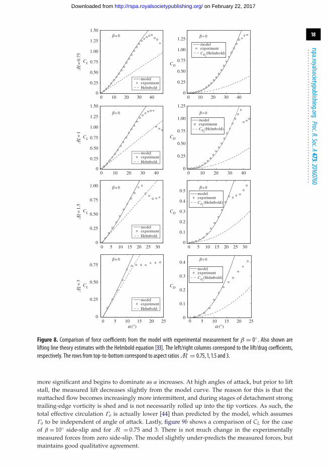
5. Model comparison and discussionIn this section, the lift, drag and rolling moment are compared with direct force/momenttransducer measurements [45]. Discussions on the various contributions to the loads, the effect ofaspect ratio and roll stall are also given. The roll moment data displayed a shift in the zero crossingcaused by the mounting strategy of the wings. Further testing showed this to be a repeatable,known bias which was removed to align the zero crossing.
Figure 8 plots the lift and drag coefficients as a function of α for the β = 0 cases. Also shownare the lifting line estimates with the Helmbold equation approximating the lift-curve slope asα → 0 (equation (4.22)). There is a rather good agreement between the model and experiment,with the former accurately capturing the vortex lift associated with the tip vortices and thereattached leading-edge shear layer flow, which cause the lift to depart from the lifting line theoryaround α = 10◦, and which is commonly observed for wings with reattached flow. The dragcoefficient begins to significantly depart from the induced-drag estimate of lifting line theoryat lower angles of attack than does the lift coefficient, and the model shows good agreementup until massive separation and lift stall occurs. For the lift, the vortex contribution quicklysubsides with increasing aspect ratio and the lift, not surprisingly, approaches the lifting lineestimate. Higher aspect ratios cannot benefit from increased lift from vortex suction, becausethe flow is unable to reattach. Because the model relies on the assumption of reattached flow,it is not expected to capture the behaviour of the aerodynamic loads beyond the massiveseparation event.
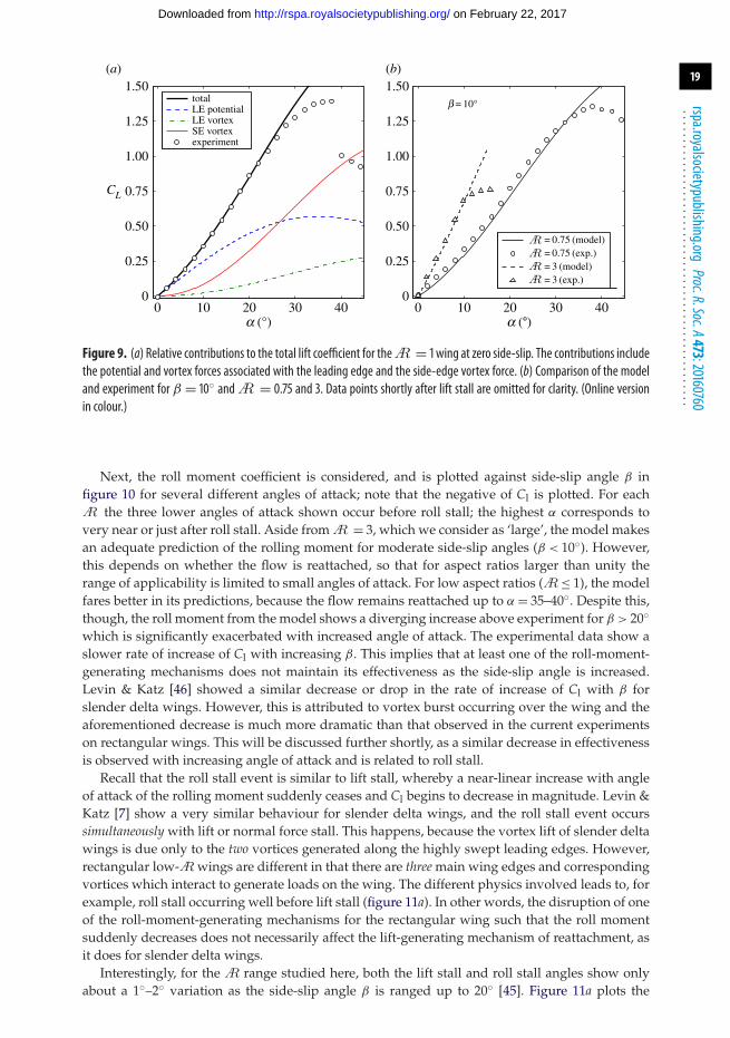
To show the relative contributions of the forces for a low-A wing, figure 9a plots the differentconstituents for CL of the A = 1 wing. It is seen that each force type provides a comparablecontribution to the total at moderate angles of attack and that the side-edge vortex force becomes
on February 22, 2017http://rspa.royalsocietypublishing.org/Downloaded from
18
rspa.royalsocietypublishing.orgProc.R.Soc.A473:20160760
...................................................
10 20 30 400
0
0.25
0.50
0.75
1.00
1.25
1.50
00
0
0
0.25
0.50
0.75
1.00
1.25
1.50
CL
CL
CL
CL
modelexperimentHelmbold
10 20 30 400
0
0.25
0.50
0.75
1.00
1.25
5 10 15 20 25
5 10 15 20 25
30 5 10 15 20 25 300
0.25
0.50
0.75
0
0.25
0.50
0.75
1.00
0
0.1
0.2
0.3
0.4
0.5
a (°) a (°)5 10 15 20 25
00
0
0
0.1
0.2
0.3
0.4
10 20 30 40 10 20 30 40
CD
0
0.25
0.50
0.75
1.00
1.25
CD
CD
CD
modelexperimentHelmbold
modelexperimentHelmbold
modelexperimentHelmbold
model
b = 0
b = 0b = 0
b = 0b = 0
b = 0b = 0
b = 0
experimentCDi
(Helmbold)
modelexperimentCDi
(Helmbold)
modelexperimentCDi
(Helmbold)
modelexperimentCDi
(Helmbold)
=0.
75=
1=
3=
1.5
Figure 8. Comparison of force coefficients from the model with experimental measurement for β = 0◦. Also shown arelifting line theory estimates with the Helmbold equation [33]. The left/right columns correspond to the lift/drag coefficients,respectively. The rows from top-to-bottom correspond to aspect ratiosA = 0.75, 1, 1.5 and 3.
more significant and begins to dominate as α increases. At high angles of attack, but prior to liftstall, the measured lift decreases slightly from the model curve. The reason for this is that thereattached flow becomes increasingly more intermittent, and during stages of detachment strongtrailing-edge vorticity is shed and is not necessarily rolled up into the tip vortices. As such, thetotal effective circulation Γo is actually lower [44] than predicted by the model, which assumesΓo to be independent of angle of attack. Lastly, figure 9b shows a comparison of CL for the caseof β = 10◦ side-slip and for A = 0.75 and 3. There is not much change in the experimentallymeasured forces from zero side-slip. The model slightly under-predicts the measured forces, butmaintains good qualitative agreement.
on February 22, 2017http://rspa.royalsocietypublishing.org/Downloaded from
19
rspa.royalsocietypublishing.orgProc.R.Soc.A473:20160760
...................................................
10 20 30 400
0
0.25
0.50
0.75
1.00
1.25
1.50
00
0.25
0.50
0.75
1.00
1.25
1.50totalLE potentialLE vortexSE vortexexperiment
= 0.75 (model)= 0.75 (exp.)= 3 (model)= 3 (exp.)
b = 10°
CL
a (°)10 20 30 40
a (°)
(b)(a)
Figure 9. (a) Relative contributions to the total lift coefficient for theA = 1 wing at zero side-slip. The contributions includethe potential and vortex forces associated with the leading edge and the side-edge vortex force. (b) Comparison of the modeland experiment for β = 10◦ andA = 0.75 and 3. Data points shortly after lift stall are omitted for clarity. (Online versionin colour.)
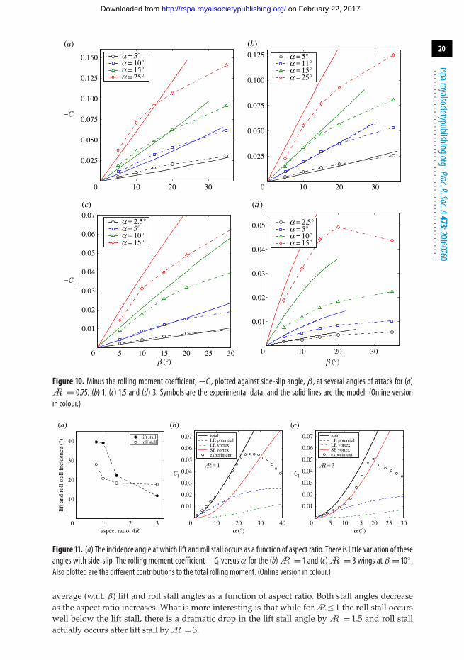
Next, the roll moment coefficient is considered, and is plotted against side-slip angle β infigure 10 for several different angles of attack; note that the negative of Cl is plotted. For eachA the three lower angles of attack shown occur before roll stall; the highest α corresponds tovery near or just after roll stall. Aside fromA = 3, which we consider as ‘large’, the model makesan adequate prediction of the rolling moment for moderate side-slip angles (β < 10◦). However,this depends on whether the flow is reattached, so that for aspect ratios larger than unity therange of applicability is limited to small angles of attack. For low aspect ratios (A≤ 1), the modelfares better in its predictions, because the flow remains reattached up to α = 35–40◦. Despite this,though, the roll moment from the model shows a diverging increase above experiment for β > 20◦which is significantly exacerbated with increased angle of attack. The experimental data show aslower rate of increase of Cl with increasing β. This implies that at least one of the roll-moment-generating mechanisms does not maintain its effectiveness as the side-slip angle is increased.Levin & Katz [46] showed a similar decrease or drop in the rate of increase of Cl with β forslender delta wings. However, this is attributed to vortex burst occurring over the wing and theaforementioned decrease is much more dramatic than that observed in the current experimentson rectangular wings. This will be discussed further shortly, as a similar decrease in effectivenessis observed with increasing angle of attack and is related to roll stall.
Recall that the roll stall event is similar to lift stall, whereby a near-linear increase with angleof attack of the rolling moment suddenly ceases and Cl begins to decrease in magnitude. Levin &Katz [7] show a very similar behaviour for slender delta wings, and the roll stall event occurssimultaneously with lift or normal force stall. This happens, because the vortex lift of slender deltawings is due only to the two vortices generated along the highly swept leading edges. However,rectangular low-Awings are different in that there are three main wing edges and correspondingvortices which interact to generate loads on the wing. The different physics involved leads to, forexample, roll stall occurring well before lift stall (figure 11a). In other words, the disruption of oneof the roll-moment-generating mechanisms for the rectangular wing such that the roll momentsuddenly decreases does not necessarily affect the lift-generating mechanism of reattachment, asit does for slender delta wings.
Interestingly, for theA range studied here, both the lift stall and roll stall angles show onlyabout a 1◦–2◦ variation as the side-slip angle β is ranged up to 20◦ [45]. Figure 11a plots the
on February 22, 2017http://rspa.royalsocietypublishing.org/Downloaded from
20
rspa.royalsocietypublishing.orgProc.R.Soc.A473:20160760
...................................................
10 20 300
0.025
0.050
0.075
0.100
0.125
0.150 a = 5°a = 10°a = 15°a = 25°
10 20 30
10 20 30
0
0.025
0.050
0.075
0.100
0.125
5 10 15 20 25 300
0.01
0.02
0.03
0.04
0.05
0.06
0.07
b (°) b (°)0
0.01
0.02
0.03
0.04
0.05
−Cl
−Cl
a = 5°a = 11°a = 15°a = 25°
a = 2.5°a = 5°a = 10°a = 15°
a = 2.5°a = 5°a = 10°a = 15°
(b)(a)
(c) (d )
Figure 10. Minus the rolling moment coefficient,−Cl , plotted against side-slip angle, β , at several angles of attack for (a)A = 0.75, (b) 1, (c) 1.5 and (d) 3. Symbols are the experimental data, and the solid lines are the model. (Online versionin colour.)
1 2 30
10
20
30
40
aspect ratio: AR
lift a
nd r
oll s
tall
inci
denc
e (°
) lift stallroll stall
10 20 30 400
0.01
0.02
0.03
0.04
0.05
0.06
0.07
a (°) a (°)
totalLE potentialLE vortexSE vortexexperiment
= 1
0 5 10 15 20 25 30
0.01
0.02
0.03
0.04
0.05
0.06
0.07 totalLE potentialLE vortexSE vortexexperiment
−Cl −Cl
(b)(a) (c)
= 3
Figure 11. (a) The incidence angle at which lift and roll stall occurs as a function of aspect ratio. There is little variation of theseangles with side-slip. The rolling moment coefficient−Cl versus α for the (b)A = 1 and (c)A = 3 wings at β = 10◦.Also plotted are the different contributions to the total rolling moment. (Online version in colour.)
average (w.r.t. β) lift and roll stall angles as a function of aspect ratio. Both stall angles decreaseas the aspect ratio increases. What is more interesting is that while forA≤ 1 the roll stall occurswell below the lift stall, there is a dramatic drop in the lift stall angle byA = 1.5 and roll stallactually occurs after lift stall byA = 3.
on February 22, 2017http://rspa.royalsocietypublishing.org/Downloaded from
21
rspa.royalsocietypublishing.orgProc.R.Soc.A473:20160760
...................................................
Figure 11b,c plots the rolling moment coefficient Cl as a function of angle of attack for theA =1 and 3 wings both at β = 10◦ side-slip; again note that the negative of Cl is plotted. Also shownare the model predictions and the different contributions to the total rolling moment. ForA = 3,the model over-predicts the measured Cl, but note that after lift stall (α ≈ 12◦) the data better alignwith the roll moment contribution from just the side-edge vortex (figure 11c). This makes sense,because at this angle of attack the leading-edge shear layer is no longer reattached and thereforeshould not be expected to create potential nor vortex lift (in the sense of the Polhamus method).The upstream side-edge vortex then generates a large moment. However, because the wing is inside-slip, the massive separation spreads across the wing towards the upstream wing edge as α
is increased further. When this separation reaches the upstream edge or sufficiently disrupts theside-edge vortex there, then roll stall occurs. This is the most likely explanation of roll stall forlarge-aspect-ratio wings; however, the mechanism is different for low aspect ratios.
For A = 1, the model predicts the rolling moment quite well prior to roll stall (figure 11b)and it is clear that the growth trend is dominated by the side-edge vortex moment. However,the model obviously does not capture the roll stall occurring at α ≈ 21◦. As such, it seems thatthe roll-moment-generating mechanism that should lose effectiveness is the side-edge vortex.However, we do not believe that this loss of effectiveness is due to vortex breakdown or bursting.The reason is because these low-A wings maintain reattached flow, and thus lift generation, upto high angles of attack, whereas vortex breakdown typically results in a detriment to the lift [47].Moreover, figure 2 shows fairly coherent (time-averaged) vortex structures.
Noting that roll stall is an abrupt change in rolling moment slope, we lastly considered that rollstall is caused by either a sudden inboard movement of the upstream TV from its respective sideedge and/or a return towards lateral flow symmetry. In the case of the latter, it is possible that thedownstream TV may regain some of its roll-moment-generating effectiveness to counteract that ofthe upstream TV. This seems plausible, because the vortex structures grow in strength with angleof attack. Moreover, this might explain why the behaviour of the decrease in Cl after roll stall issimilar to the way it increases from low angles of attack (recall figure 11b). Another factor is thatlocally separated flow may reattach owing to an increased downwash of the side-edge vorticeswith angle of attack. However, more work is necessary to determine the exact mechanism of rollstall for low-Awings.
6. Concluding remarksThe mean flow field around a low-A rectangular wing at α = 35◦ and Re = 80 000 for differentside-slip angles of β = 0◦, 10◦, 20◦, 35◦ was measured with S-DPIV. The side-slip condition wasstudied as it has major implications on the lateral loads and dynamics of low-A fliers. Theobjective was to obtain information on the local flow, particularly the vortex structure. Theexperimental observations were then used to validate high-angle of attack assumptions madein a very simplified model for the aerodynamic loads on the wings.
The development of the model begins with a new interpretation of slender body theory inthe limit as the span of a rectangular wing approaches zero and such that its side-edge vorticesmerge into a vortex doublet or dipole with variable strength in the streamwise direction. Fromthis, we theoretically derived a parabolic spanwise loading, instead of the elliptic distributionassociated with fully attached flow in classical aerodynamics. The experimental measurementsof the spanwise circulation distribution very closely displayed this parabolic behaviour. Thephysical explanation is that there is an additional circulation around the wing associated with thereattached flow that comprises the leading-edge separation region. This is a fundamental featureof wings with a broad-facing leading edge and represents a differentiation from delta wings aswell as rectangular wings at small incidence. Additionally, the potential solution provides anexpression for the dynamic pressure associated with the downwash of the tip vortices that acts toreattach the leading-edge shear layer.
Another interpretation of the slender body potential flow model is to consider it as the zero-aspect-ratio limit of a horseshoe vortex, which is perhaps the simplest representation of a wing. In
on February 22, 2017http://rspa.royalsocietypublishing.org/Downloaded from
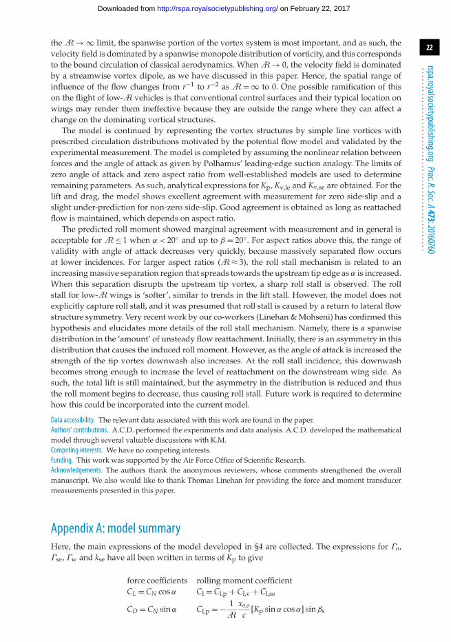
22
rspa.royalsocietypublishing.orgProc.R.Soc.A473:20160760
...................................................
theA→ ∞ limit, the spanwise portion of the vortex system is most important, and as such, thevelocity field is dominated by a spanwise monopole distribution of vorticity, and this correspondsto the bound circulation of classical aerodynamics. WhenA→ 0, the velocity field is dominatedby a streamwise vortex dipole, as we have discussed in this paper. Hence, the spatial range ofinfluence of the flow changes from r−1 to r−2 asA= ∞ to 0. One possible ramification of thison the flight of low-A vehicles is that conventional control surfaces and their typical location onwings may render them ineffective because they are outside the range where they can affect achange on the dominating vortical structures.
The model is continued by representing the vortex structures by simple line vortices withprescribed circulation distributions motivated by the potential flow model and validated by theexperimental measurement. The model is completed by assuming the nonlinear relation betweenforces and the angle of attack as given by Polhamus’ leading-edge suction analogy. The limits ofzero angle of attack and zero aspect ratio from well-established models are used to determineremaining parameters. As such, analytical expressions for Kp, Kv,le and Kv,se are obtained. For thelift and drag, the model shows excellent agreement with measurement for zero side-slip and aslight under-prediction for non-zero side-slip. Good agreement is obtained as long as reattachedflow is maintained, which depends on aspect ratio.
The predicted roll moment showed marginal agreement with measurement and in general isacceptable forA≤ 1 when α < 20◦ and up to β = 20◦. For aspect ratios above this, the range ofvalidity with angle of attack decreases very quickly, because massively separated flow occursat lower incidences. For larger aspect ratios (A≈ 3), the roll stall mechanism is related to anincreasing massive separation region that spreads towards the upstream tip edge as α is increased.When this separation disrupts the upstream tip vortex, a sharp roll stall is observed. The rollstall for low-A wings is ‘softer’, similar to trends in the lift stall. However, the model does notexplicitly capture roll stall, and it was presumed that roll stall is caused by a return to lateral flowstructure symmetry. Very recent work by our co-workers (Linehan & Mohseni) has confirmed thishypothesis and elucidates more details of the roll stall mechanism. Namely, there is a spanwisedistribution in the ‘amount’ of unsteady flow reattachment. Initially, there is an asymmetry in thisdistribution that causes the induced roll moment. However, as the angle of attack is increased thestrength of the tip vortex downwash also increases. At the roll stall incidence, this downwashbecomes strong enough to increase the level of reattachment on the downstream wing side. Assuch, the total lift is still maintained, but the asymmetry in the distribution is reduced and thusthe roll moment begins to decrease, thus causing roll stall. Future work is required to determinehow this could be incorporated into the current model.
Data accessibility. The relevant data associated with this work are found in the paper.Authors’ contributions. A.C.D. performed the experiments and data analysis. A.C.D. developed the mathematicalmodel through several valuable discussions with K.M.Competing interests. We have no competing interests.Funding. This work was supported by the Air Force Office of Scientific Research.Acknowledgements. The authors thank the anonymous reviewers, whose comments strengthened the overallmanuscript. We also would like to thank Thomas Linehan for providing the force and moment transducermeasurements presented in this paper.
Appendix A: model summaryHere, the main expressions of the model developed in §4 are collected. The expressions for Γo,Γse, Γw and kse have all been written in terms of Kp to give
force coefficients rolling moment coefficientCL = CN cos α Cl = Cl,p + Cl,v + Cl,se
CD = CN sin α Cl,p = − 1A
xo,s
c[Kp sin α cos α] sin βs
on February 22, 2017http://rspa.royalsocietypublishing.org/Downloaded from
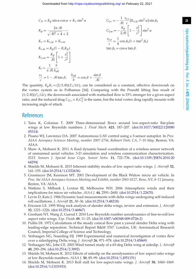
23
rspa.royalsocietypublishing.orgProc.R.Soc.A473:20160760
...................................................
CN = Kp sin α cos α + Kv sin2 α Cl,v = − 1A
xo,s
c[Kv,le sin2 α] sin βs
Kp = 2πA√A2 + 4 + 2
Cl,se = − Kp
2A
[1 − x2
1c2
]sin2 α
Kv = Kv,le + Kv,sexo,s
c= 1
4cos βs(1 + tan2 βs)
Kv,le = Kp(1 − KiKp) tan βs = cos α tan β.
Kv,se = Kp
A
[1 + x2
1c2
]
Ki = 1πA
bbeff
x1
c= 1 −A tan β,
beff
b= cos β + sin β
A.
The quantity, KpKi = (2/3A)(Γo/Uc), can be considered as a constant, effective downwash onthe vortex system as in Polhamus [16]. Comparing with the Prandtl lifting line result of(1/2A)(Γo/Uc), the downwash associated with reattached flow is 33% stronger for a given aspectratio, and the induced drag CD,i = KiC2
L is the same, but the total vortex drag rapidly mounts withincreasing angle of attack.
References1. Taira K, Colonius T. 2009 Three-dimensional flows around low-aspect-ratio flat-plate
wings at low Reynolds numbers. J. Fluid Mech. 623, 187–207. (doi:10.1017/S0022112008005314)
2. Pisano WJ, Lawrence DA. 2007 Autonomous UAV control using a 3-sensor autopilot. In Proc.AIAA Aerospace Sciences Meeting, number 2007-2756, Rohnert Park, CA, 7–10 May. Reston, VA:AIAA.
3. Shaw A, Mohseni K. 2011 A fluid dynamic based coordination of a wireless sensor networkof unmanned aerial vehicles: 3-D simulation and wireless communication characterization.IEEE Sensors J. Special Issue Cogn. Sensor Netw. 11, 722–736. (doi:10.1109/JSEN.2010.2064294)
4. Shields M, Mohseni K. 2015 Inherent stability modes of low aspect ratio wings. J. Aircraft 52,141–155. (doi:10.2514/1.C032636)
5. Grasmeyer JM, Keennon MT. 2001 Development of the Black Widow micro air vehicle. InProc. the AIAA Aerospace Sciences Meeting and Exhibit, number 2001-0127, Reno, NV, 8–11 January.Reston, VA: AIAA.
6. Watkins S, Milbank J, Loxton BJ, Melbourne WH. 2006 Atmospheric winds and theirimplications for micro air vehicles. AIAA J. 44, 2591–2600. (doi:10.2514/1.22670)
7. Levin D, Katz J. 1984 Dynamic load measurements with delta wings undergoing self-inducedroll oscillations. J. Aircraft 21, 30–36. (doi:10.2514/3.48218)
8. Ericsson LE. 1995 Wing rock analysis of slender delta wings, review and extension. J. Aircraft32, 1221–1226. (doi:10.2514/3.46867)
9. Gresham NT, Wang Z, Gursul I. 2010 Low Reynolds number aerodynamics of free-to-roll lowaspect ratio wings. Exp. Fluids 49, 11–25. (doi:10.1007/s00348-009-0726-2)
10. Pullin DI. 1972 Calculations of the steady conical flow past a yawed slender Delta wing withleading-edge separation. Technical Report R&M 3767. London, UK: Aeronautical ResearchCouncil, Imperial College of Science and Technology.
11. Verhaagen NG, Naarding HJ. 1989 Experimental and numerical investigation of vortex flowover a sideslipping Delta wing. J. Aircraft 26, 971–978. (doi:10.2514/3.45869)
12. Verhaagen NG, Jobe CE. 2003 Wind tunnel study of a 65-deg Delta wing at sideslip. J. Aircraft40, 290–296. (doi:10.2514/2.3092)
13. Shields M, Mohseni K. 2012 Effects of sideslip on the aerodynamics of low aspect ratio wingsat low Reynolds numbers. AIAA J. 50, 85–99. (doi:10.2514/1.J051151)
14. Shields M, Mohseni K. 2013 Roll stall for low-aspect-ratio wings. J. Aircraft 50, 1060–1069.(doi:10.2514/1.C031933)
on February 22, 2017http://rspa.royalsocietypublishing.org/Downloaded from
24
rspa.royalsocietypublishing.orgProc.R.Soc.A473:20160760
...................................................
15. Shields M, Mohseni K. 2013 Passive mitigation of roll stall for low aspect ratio wings. Adv.Robot. 27, 667–681. (doi:10.1080/01691864.2013.778941)
16. Polhamus EC. 1966 A concept of the vortex lift of sharp-edge delta wings based on a leading-edge suction analogy. Technical Report TN D-3767. Hampton, VA: NASA, Langley ResearchCenter.
17. Soloff SM, Adrian RJ, Liu ZC. 1997 Distortion compensation for generalized stereoscopicparticle image velocimetry. Meas. Sci. Technol. 8, 1441–1454. (doi:10.1088/0957-0233/8/12/008)
18. Willert C. 1997 Stereoscopic digital particle image velocimetry for application in wind tunnelflows. Meas. Sci. Technol. 8, 1465–1479. (doi:10.1088/0957-0233/8/12/010)
19. Wieneke B. 2005 Stereo-PIV using self-calibration on particle images. Exp. Fluids 39, 267–280.(doi:10.1007/s00348-005-0962-z)
20. Westerweel J. 2000 Theoretical analysis of the measurement precision in particle imagevelocimetry. Exp. Fluids 29, S3–S12. (doi:10.1007/s003480070002)
21. Raffel M, Willert CE, Kompenhans J. 1998 Particle image velocimetry. New York City, NY:Springer.
22. Yilmaz TO, Rockwell D. 2010 Three-dimensional flow structure on a maneuvering wing. Exp.Fluids 48, 539–544. (doi:10.1007/s00348-009-0772-9)
23. Visbal. MR. 2011 Three-dimensional flow structure on a headving low-aspect-ratio wing. InProc. 49th AIAA Aerospace Sciences Meeting, number 2011-219, Orlando, FL, 4–7 January, pp. 1–24.Reston, VA: AIAA.
24. Jian T, Ke-Qin Z. 2004 Numerical and experimental study of flow structure of low-aspect-ratiowings. J. Aircraft 41, 1196–1201. (doi:10.2514/1.5467)
25. Wu JZ, Wu JM, Wu CJ. 1987 A general three-dimensional viscous compressible theory on theinteraction of solid body and vorticity-dilatation field. Technical Report UTSI Report 87/03.Tullahoma, TN: University of Tennessee Space Institute.
26. Perry AE, Chong MS. 1994 Topology of flow patterns in vortex motions and turbulence. Appl.Sci. Res. 53, 357–374. (doi:10.1007/BF00849110)
27. DeVoria AC, Ringuette MJ. 2012 Vortex formation and saturation for low-aspect-ratio rotatingflat-plate fins. Exp. Fluids 52, 441–462. (doi:10.1007/s00348-011-1230-z)
28. Gursul I, Gordnier R, Visbal M. 2005 Unsteady aerodynamics of nonslender delta wings. Prog.Aerosp. Sci. 41, 515–557. (doi:10.1016/j.paerosci.2005.09.002)
29. Prandtl L. 1921 Applications of modern hydrodynamics to aeronautics. Technical report no.116. National Advisory Committee for Aeronautics.
30. Bollay W. 1939 A nonlinear wing theory and its application to rectangular wings of smallaspect ratio. Z. Agnew. Math. Mech. 19, 21–35. (doi:10.1002/zamm.19390190103)
31. Falkner VM. 1943 The calculation of aerodynamic surfaces of any shape. Report ARC R&M1910. London, UK: Ministry of Technology.
32. Jones RT. 1946 Properties of low-aspect-ratio pointed wings at speeds below and above thespeed of sound. J. Eng. Math. 19, 157–172.
33. Helmbold HB. 1942 Der unvurwundene ellipsenfliigel als tragende fliiche. Report, derDeutschen Luftfahrt-forschung, R. Oldenbourg (Munich).
34. Küchemann D. 1956 Der unvurwundene ellipsenfliigel als tragende fliiche. Report no. 2935,Ministry of Supply.
35. Brown CE, Michael WH. 1954 Effect of leading-edge separation on the lift of a delta wing.J. Aeronaut. Sci. 21, 690–694. (doi:10.2514/8.3180)
36. Mangler KW, Smith JHB. 1959 A theory of the flow past a slender delta wing with leadingedge separation. Proc. R. Soc. Lond. A 251, 200–217. (doi:10.1098/rspa.1959.0102)
37. Lamar JE. 1974 Extension of leading-edge suction analogy to wings with separated flowaround the side edges at subsonic speeds. Technical Report TR R-428. Hampton, VA: NASA,Langley Research Center.
38. Multhopp H. 1950 Methods for calculating the lift distribution of wings (subsonic lifting-surface theory). Report no. 29884, Ministry of Supply.
39. Riley N, Smith JHB. 1985 Prediction of leading-edge behavior to supplement the suctionanalogy. J. Eng. Math. 19, 157–172. (doi:10.1007/BF00042738)
40. Clark RW, Smith JHB, Thompson CW. 1975 Some series expansion solutions for slender wingswith leading-edge separation. Report ARC R&M 3785. London, UK: Ministry of Defence.
41. Cole JD. 1968 Perturbation methods in applied mathematics, 1st edn. Waltham, MA: BlaisdellPublishing Company.
on February 22, 2017http://rspa.royalsocietypublishing.org/Downloaded from
25
rspa.royalsocietypublishing.orgProc.R.Soc.A473:20160760
...................................................
42. Hemsch MJ, Luckring JM. 1990 Connection between leading-edge sweep, vortex lift, andvortex strength for delta wings. J. Aircraft 27, 473–475. (doi:10.2514/3.25305)
43. Milne-Thomson LM. 1958 Theoretical aerodynamics. Mineola, NY: Dover.44. DeVoria AC, Mohseni K. 2017 On the mechanism of high-incidence lift generation for steadily
translating low-aspect-ratio wings. J. Fluid Mech. 813, 110–126. (doi:10.1017/jfm.2016.849)45. Linehan T, Mohseni K. 2016 Aerodynamics and lateral stability of low-aspect-ratio wings with
dihedral at low Reynolds numbers. In Proc. AIAA Aerospace Sciences Meeting, number 2016-1063, San Diego, CA, 4–8 January. Reston, VA: AIAA.
46. Katz J, Levin D. 1991 Static measurements of slender delta wing rolling moment hysteresis.J. Aircraft 28, 282–283. (doi:10.2514/3.46024)
47. Gursul I. 2005 Review of unsteady vortex flows over slender delta wings. J. Aircraft 42,299–319. (doi:10.2514/1.5269)
on February 22, 2017http://rspa.royalsocietypublishing.org/Downloaded from