Embed Size (px)
Citation preview
IOSR Journal of Applied Geology and Geophysics (IOSR-JAGG)
e-ISSN: 2321–0990, p-ISSN: 2321–0982.Volume 2, Issue 2 Ver. II. (Mar-Apr. 2014), PP 08-17
www.iosrjournals.org
www.iosrjournals.org 8 | Page
AVO inversion and Lateral prediction of reservoir properties of
Amangi hydrocarbon field of the Niger Delta area of Nigeria
Sonny Inichinbia1, Peter O. Sule
2, Aminu L. Ahmed
2 and *Halidu Hamza
2
1Department of Physics, Ahmadu Bello University, Zaria, Nigeria
2Department of Physics, Ahmadu Bello University, Zaria, Nigeria
*2Department of Geology, Ahmadu Bello University, Zaria, Nigeria
Abstract: Well log modelling was performed using a complete suite of compressional, shear and density logs to
understand and determine the expected angle dependent effects in the seismic reflection data and also to
estimate wavelets for the different input stacks. The available well controls were used in wavelet estimation and
we incorporated AVO modelling to properly account for AVO effects. We partitioned the 3D seismic reflection
data into three partial angle stacks of near (0o – 10
o), mid (11
o – 20
o) and far (21
o – 30
o). Wavelets were
estimated separately for each angle stack to enable the inversion to compensate for offset dependent phase,
bandwidth, tuning and normal moveout (NMO) stretch effects which could affect the amplitude and phase
spectra of the data. We then simultaneously inverted multiple angle stacks to transform P-wave offset seismic
reflection data to P-impedance and S-impedance volumes. These impedance volumes were interpreted
separately. This method supported interpretation in this field where the reservoirs’ sandstones and shales
cannot be distinguished from the P- impedance alone.
Keywords: Angle stacks, AVO inversion, crossplot analysis, P -impedance, S-impedance,
I. Introduction The field was discovered by well-002 which was drilled in 1992 and was initially covered in that same
year by a 2D seismic survey that was reprocessed in 2005. Imaging of the crest of the structure remained very
poor. Uncertainties about the lateral extent, pinchout, distribution of reservoir properties (such as porosity, net
pay thickness, fluid type and fluid saturation, etc), and fault positions along the reservoirs are some challenges
that are not yet fully understood in the Amangi Field. Hence, some of the risks associated with the field are
fault/seal integrity, sand development/reservoir development, overpressures and reservoir rock properties. There
are also exploration challenges in the data set of the field, such as the discrimination of hydrocarbon bearing
sands from shales and more importantly, the separation of gas sands from water (brine) saturated sandstones.
However, the promising domestic gas potential of this field calls for improvement in the interpretation
of very deep seismic events and valid estimates of the reservoirs properties. In order to address these issues, new
3D seismic data was acquired with long offset cable and high fold of coverage giving better resolution and
structural interpretation across the reservoirs of interest compared to earlier dataset. The current challenge is
therefore; to use the new processed anisotropic 3D prestack seismic data to derisk the reservoirs lateral extent,
variability and heterogeneity and select location for new development wells. This research is intended to achieve
these results by the application of rock physics, seismic AVO and inversion attributes.
Just as these reservoirs under consideration, most hydrocarbon reservoirs of the Niger Delta are
heterogeneous. Sources of reservoir heterogeneity include variations in lithology, porosity, permeability, and
pore fluid properties. They control not only the amount of hydrocarbons that may be present but also their
recoverability from distributed reservoir compartments. As such, reservoir heterogeneities are the primary
causes of low hydrocarbon recovery efficiency, resulting in poor sweep, early breakthrough, and pockets of
bypassed oil. Several interpretation techniques have emerged to map rock and fluid spatial variability. These
techniques include estimates of lithology, porosity, and saturation from geologic, well log, and seismic data.
Inversion of Amplitude Variation with Offset (AVO) results provides elastic rock properties which can be used
to determine lithology and fluid content of reservoirs.
In this paper this approach is demonstrated using a case study of Amangi field of the Niger Delta of
Nigeria. The ultimate goal of this study was to obtain reliable quantitative estimate of relevant reservoir rock
and fluid parameters in the area. The major components of our study are: (1) Well log analysis to define
different seismic lithofacies, rock physics analysis including fluid effects and log based analysis of near offset
and far offset seismic attributes for different lithofacies and pore fluids (2) Seismic inversion of near offset and
far offset partial stacks to obtain inversion volumes of near offset and far offset impedances. Seismic inversion
of near offset and far offset stacks gave us two volumes of impedance attributes of the field. The near offset
stack approximates a zero offset section, giving an estimate of the normal incidence acoustic impedance. The far
AVO inversion and Lateral prediction of reservoir properties of Amangi hydrocarbon field of the
www.iosrjournals.org 9 | Page
offset stack gave an estimate of a Vp/Vs related elastic impedance attribute that is equivalent to the acoustic
impedance for non normal incidence.
Inverting geophysical data for reservoir properties of interest requires linking the underlying geology to
the observed data. In order to do so, the geologic heterogeneity needs to be modelled to examine how it controls
the reservoir properties and affects any geophysical measurements [1]. A successful seismic based reservoir
properties estimation effort has three steps: accurate seismic inversion in 3D to obtain relevant reservoir
parameters, rock physics transformation to relate reservoir parameters to the seismic parameters, and mapping
these parameters in 3D. This problem is nonunique and thus any available information, especially geologic
interpretation should be used to improve our ability to infer the reservoir properties of interest with confidence
[2].
Amangi field was covered by a surface anisotropic 3D seismic survey that was specially processed for
amplitude interpretation. [3] defined seismic lithofacies as representing seismic scale sedimentary units with
distinguishable characteristic petrophysical properties such as clay content, bedding configuration (massive or
interbedded), petrography (grain size, cementation, packing, clay location), and seismic properties (P-wave
velocity, S-wave velocity, and density). Linking 3D seismic data with rock physics properties of different facies
and pore fluids can provide a powerful strategy for improved quantitative interpretation the of seismic data. This
was the basis for quantitative facies and fluid estimation from seismic data. Seismic scale here refers to units
that can be observed and mapped from seismic data. This depends on vertical and lateral seismic resolution
which is governed by wavelength, Fresnel zone radius and depth to target. In this study, the wavelength was
about 60m and the thickness of the seismic lithofacies units are on the order of 25 m - 81 m.
II. Field location and geology Amangi Field is located 70 km northwest of Port Harcourt within licence OML 21 of the Niger Delta
of southern Nigeria as shown in Figure 1. The field measures 12 km x 5 km and is still a prospect which has not
yet been fully appraised. The Niger Delta lies between latitudes 4° N and 6° N and longitudes 3° E and 9° E.
The structure of Amangi field is an elongated rollover anticline bounded to the south and southeast by large
boundary faults that throw down towards the south and southeast. Towards the north is a regional growth fault
that joins with the northeastern boundary fault to close the structure towards the east. It is a fault dip closure
against a large growth fault which separates it from a neighbouring field.
The H4000 hydrocarbons are trapped in a closure against the southern and southeastern faults. The
structure is bounded to the south and to the southwest by large faults that throw down towards the south and
southeast. It is bounded to the north and south by large listric normal faults associated with gravity collapse in
the delta. The western aquifer part of the structure is not covered by the 3D seismic data, but the fact that the
reservoirs are overpressured suggests another bounding fault there.
Figure 1. Map of the Niger Delta showing the study area. The encircled portion is the location of Amangi
Field. (Source: Shell Petroleum Development Company of Nigeria Ltd.).
III. Well data The location of the wells in the field is displayed in Fig. 2. A total of four wells are sited in OML 21
while only two wells are sited in OML 53.

AVO inversion and Lateral prediction of reservoir properties of Amangi hydrocarbon field of the
www.iosrjournals.org 10 | Page
Figure 2. OML map of the study area showing the locations of the wells used in this study. Four out of a
total of six wells are located in OML 21 whereas the rest two wells are sited in OML 53.
Well logs play an important role of linking rock parameters to the seismic data. A key well was
identified with a complete suite of good quality logs that sampled all of the important lithologies in the field.
Figure 2 shows an example of some of the important logs from the key well. Reasons for choosing this well as
the key well are that shear wave information is available, the important facies of the turbidite system are all
encountered in the well, and it is a new well with good quality modern logs. The gamma-ray log values and
patterns, and velocity and density logs were used primarily to determine the different facies with contrasting
seismic properties.
Figure 3. Porosity, volume shale, gamma ray, calliper, P and S sonic, resistivity, density, porosity,
neutron-density, VP , and VS logs from one of the key wells used in this study.
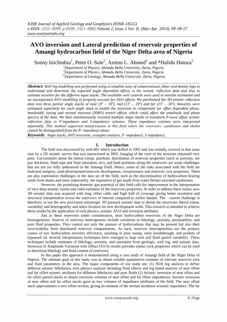
IV. Seismic data Amangi field was covered by a 3D seismic survey between 2008 and 2010 which was processed in
2011. The data is reasonably good down to 2.5 seconds, beyond which deeper events are poorly defined and
discontinuous as shown in Fig. 4.
AVO inversion and Lateral prediction of reservoir properties of Amangi hydrocarbon field of the
www.iosrjournals.org 11 | Page
Figure 4. Processed seismic section of Amangi field with well-001 and well-002 superimposed (courtesy:
SPDC).
V. Methodology Firstly, well log modelling was undertaken to understand the angle dependent effects in the 3D seismic
reflection data and estimate the wavelets for the different input angle stacks. For the well log modelling a full
suite of logs (Vp, Vs, and ρ) were used. Vs was obtained from Vp using Greenberg-Castagna relationship. Fluid
fill and angles of incidence were modelled to model the expected AVO effects and the angles of incidence for
which they were observed. Next, Crossplot analysis was applied to evaluate the discriminating power of the
elastic logs and their transforms. With the estimated wavelets for each angle stack, velocity model, interpreted
seismic horizons and available well control the seismic reflection data were inverted for rock property
evaluation, following [4].
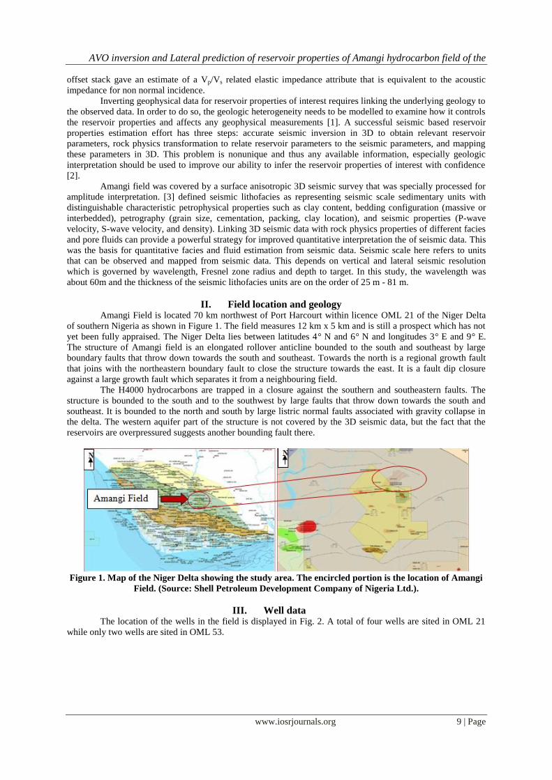
VI. Results and discussions We first undertook crossplot analysis to discriminate the reservoir properties of the field. Fig. 5 shows
the seismic lithofacies defined from the wells and by fluid substitution in an acoustic or P-impedance versus S-
impedance crossplot. These data points are from a depth around 2,702 m and 2,919 m. Lithofacies that
overlapped in the acoustic impedance domain were discriminated by their elastic or S-impedance as shown in
Fig. 5.
Figure 5. Crossplot of S-impedance versus P- impedance for different lithofacies. Yellow markers indicate
gas saturated facies and Green and red colours indicate shale while light blue corresponds to brine
saturated facies. Facies that overlap in P- impedance are clearly discriminated by their S-impedance.
P-impedance alone could not discriminate sand from shale. This suggests to us that full stack
constrained sparse spike inversion (CSSI) could not separate sand from shale. So, we resorted to using
RockTrace AVO inversion using non overlapping partial angle stacks. Crossplots of acoustic impedance versus
Vp/Vs ratio and porosity color coded to gamma ray is one way to visualize the lithologic information present in

AVO inversion and Lateral prediction of reservoir properties of Amangi hydrocarbon field of the
www.iosrjournals.org 12 | Page
the data. Fig. 6 shows that the porosity is relatively constant within this depth interval, and the shale has both a
high acoustic impedance equivalent to the sands and higher Vp/Vs ratio than the sands. Brine sands and gas
sands were grouped as separate categories.
Thus from AVO analysis we are able distinguish the gas sand from brine sand and shale with the Vp/Vs
versus P-impedance crossplot. Gas saturated sands in well-002 show some amount of increase in P-impedance.
But the P-impedance space alone could not adequately delineate the rock types because of a reasonably large
degree of overlap in the P-impedance value of the rock units. However, the shale dominated section and the
sand dominated section are clearly identified and separated on the plot in the Vp/Vs domain. So, the Vp/Vs space
proved adequate in separating the different rock types, as shown in Fig. 6.
Note that the hydrocarbon sands span Vp/Vs ratio from 1.65 – 1.80, indicating some intercalation of
shale within the reservoirs. The Vp/Vs cut-off here is 1.8. Thus, decrease in net-to-gross (N/G) causes a drastic
increase of Vp/Vs and very little shale intercalation will cause a significant increase in Vp/Vs compared to
homogeneous, clean sands (net-to-gross = 1). We used the reservoir sand together with some interval of the
sealing shale in the crossplots, and we can clearly observe that the gas saturated sands span a wide range of
Vp/Vs ratios, even close to 1.8. An inverted Vp/Vs section superimposed with the wells in the area of study is
displayed in Figure 4, to further buttress this point. Hydrocarbon sands have Vp/Vs ratio ranging from 1.6 to 1.9.
Gas saturated sands are clearly separated from the shales.
Figure 6. Rock properties as a function of seismic parameters: acoustic impedance versus Vp/Vs color
coded to gamma ray (left) and porosity (right). On the left, the shalier points (red and green have both a
lower acoustic impedance and higher Vp/Vs ratio than the sands (yellow). The porosity is higher in the
sands than the shales (right).
An important complicating factor is the presence of flushed zones in hydrocarbon columns at the wells.
Because of the water based drilling fluid, the well logs could be measuring water saturated rocks from the mud-
filtrate invaded zone instead of measuring the gas saturated rocks. This was carefully investigated using deep
sounding and shallow sounding resistivity and Gassmann modelling.
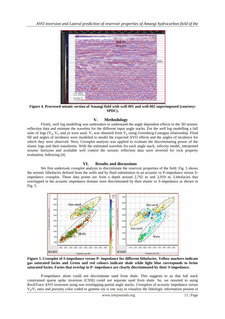
Fig. 7 illustrates changes in seismic response when the gas saturated reservoirs were replaced by brine.
The synthetics are calculated along a normal incidence and zero offset trajectory. The gas saturation is set at
80%. The brine case shows brightening of the reflection with respect to the gas filled scenario because the
H1000 sand has higher P-impedance than the encasing shales and is “hard” sand displaying increased amplitude
and reversal of phase at the top of the reservoir sands. Both the H1000 and H4000 reservoirs showed this
increased contrast tendency, because both sands have higher P-impedance than the encasing shales. There is a
decrease in Vp, Vs and density indicating the presence of gas and porosity of the reservoir.
AVO inversion and Lateral prediction of reservoir properties of Amangi hydrocarbon field of the
www.iosrjournals.org 13 | Page
Figure 7. Gassmann fluid substitution and synthetics generation at normal incidence, modelling seismic
responses at the reservoirs tops. Fluid substitution to brine makes H1000 harder than insitu condition
and Fluid substitution to brine makes H4000 softer than insitu condition.
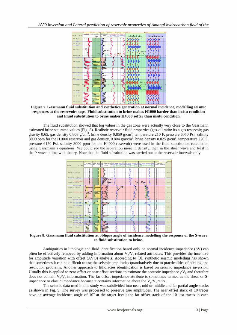
The fluid substitution showed that log values in the gas zone were actually very close to the Gassmann
estimated brine saturated values (Fig. 8). Realistic reservoir fluid properties (gas-oil ratio: its a gas reservoir; gas
gravity 0.65, gas density 0.808 g/cm3, brine density 0.859 g/cm
3, temperature 210 F, pressure 6050 Psi, salinity
8000 ppm for the H1000 reservoir and gas density, 0.804 gm/cm3, brine density 0.825 g/cm
3, temperature 220 F,
pressure 6150 Psi, salinity 8000 ppm for the H4000 reservoir) were used in the fluid substitution calculation
using Gassmann’s equations. We could see the separation more in density, then in the shear wave and least in
the P-wave in line with theory. Note that the fluid substitution was carried out at the reservoir intervals only.
Figure 8. Gassmann fluid substitution at oblique angle of incidence modelling the response of the S-wave
to fluid substitution to brine.
Ambiguities in lithologic and fluid identification based only on normal incidence impedance (ρV) can
often be effectively removed by adding information about Vp/Vs related attributes. This provides the incentive
for amplitude variation with offset (AVO) analysis. According to [3], synthetic seismic modelling has shown
that sometimes it can be difficult to use the seismic amplitudes quantitatively due to practicalities of picking and
resolution problems. Another approach to lithofacies identification is based on seismic impedance inversion.
Usually this is applied to zero offset or near offset sections to estimate the acoustic impedance ρVp and therefore
does not contain Vp/Vs information. The far offset impedance attribute is sometimes termed as the shear or S-
impedance or elastic impedance because it contains information about the Vp/Vs ratio.
The seismic data used in this study was subdivided into near, mid or middle and far partial angle stacks
as shown in Fig. 9. The survey was processed to preserve true amplitudes. The near offset stack of 10 traces
have an average incidence angle of 10o at the target level; the far offset stack of the 10 last traces in each

AVO inversion and Lateral prediction of reservoir properties of Amangi hydrocarbon field of the
www.iosrjournals.org 14 | Page
common-mid-point (CMP) gather has an average incidence angle of 30o. The 3D seismic survey covered
approximately 350 km2.
Figure 9. The Near (0
o-10
o), Middle- Mid (11
o-20
o) and Far (21
o-30
o) angle stacks used in this study.
The inline spacing was 25 m, crossline spacing 25 m, sample rate was 4 ms. The anisotropic 3D
prestack seismic data were depth migrated using a Kirchhoff algorithm and flattened using nonhyperbolic
correction beyond 30o incidence angle in Fig. 10.
Figure 10. Normal Moveout (NMO) corrected and flattened gathers.
This moveout correction yielded a high quality set of flat gathers that were stacked in selected non
overlapping angle ranges (near 0o – 10
o, medium 11
o – 20
o, and far 21
o – 30
o), to highlight amplitude variations
with offset/angle. This consistent relatively high fold in the angle ranges produced high signal-to-noise stacks.
These angle stacks are used for wavelet extraction [5].
VII. Inversion Industry proprietary constrained sparse spike algorithm was used to invert the seismic data (three
volumes of angle stacks) to P-impedance and Vp/Vs ratio. The prestack inversion was performed using Jason
Geoscience Workbench (JGW) version 8.2 package. The inversion requires as inputs information about the
seismic wavelet, the geometric structure from structural seismic interpretation, interpreted horizons and a prior
model based on well log impedance. The prior model was created by extrapolation of well data along the
defined structural horizons. The same method was used for both the near offset and far offset stacks. We
obtained a reliable estimate of the wavelet for the inversion through the software package, based on the
amplitude spectrum of a selected time window, and a scan of the phases to pick one that best matches synthetic
and true seismic traces.
A density volume was also computed, but in accordance with common practice was treated as a
byproduct and not used further. We used two well defined horizons for this purpose, H1000 and H4000. The
inversion itself is a 1D trace-by-trace inversion, based on convolution with the wavelet, followed by a
minimization of the squared error between the synthetic seismogram and the observed seismogram. A different
wavelet is used for the near offset and far offset inversions. Fig. 11 and 12 show the near offset and far offset
impedance volumes (i.e., P and S impedances) from the inversions. They are the results for a seismic line
H1000
AVO inversion and Lateral prediction of reservoir properties of Amangi hydrocarbon field of the
www.iosrjournals.org 15 | Page
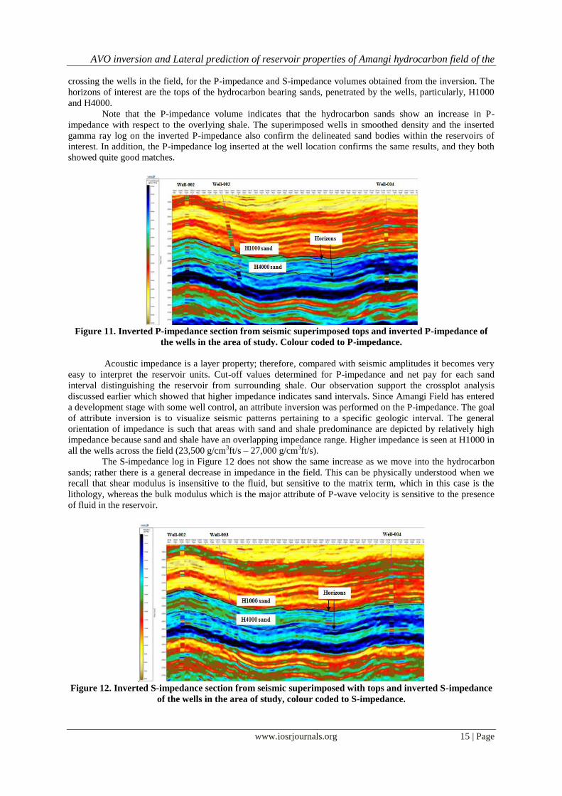
crossing the wells in the field, for the P-impedance and S-impedance volumes obtained from the inversion. The
horizons of interest are the tops of the hydrocarbon bearing sands, penetrated by the wells, particularly, H1000
and H4000.
Note that the P-impedance volume indicates that the hydrocarbon sands show an increase in P-
impedance with respect to the overlying shale. The superimposed wells in smoothed density and the inserted
gamma ray log on the inverted P-impedance also confirm the delineated sand bodies within the reservoirs of
interest. In addition, the P-impedance log inserted at the well location confirms the same results, and they both
showed quite good matches.
Figure 11. Inverted P-impedance section from seismic superimposed tops and inverted P-impedance of
the wells in the area of study. Colour coded to P-impedance.
Acoustic impedance is a layer property; therefore, compared with seismic amplitudes it becomes very
easy to interpret the reservoir units. Cut-off values determined for P-impedance and net pay for each sand
interval distinguishing the reservoir from surrounding shale. Our observation support the crossplot analysis
discussed earlier which showed that higher impedance indicates sand intervals. Since Amangi Field has entered
a development stage with some well control, an attribute inversion was performed on the P-impedance. The goal
of attribute inversion is to visualize seismic patterns pertaining to a specific geologic interval. The general
orientation of impedance is such that areas with sand and shale predominance are depicted by relatively high
impedance because sand and shale have an overlapping impedance range. Higher impedance is seen at H1000 in
all the wells across the field (23,500 g/cm3ft/s – 27,000 g/cm
3ft/s).
The S-impedance log in Figure 12 does not show the same increase as we move into the hydrocarbon
sands; rather there is a general decrease in impedance in the field. This can be physically understood when we
recall that shear modulus is insensitive to the fluid, but sensitive to the matrix term, which in this case is the
lithology, whereas the bulk modulus which is the major attribute of P-wave velocity is sensitive to the presence
of fluid in the reservoir.
Figure 12. Inverted S-impedance section from seismic superimposed with tops and inverted S-impedance
of the wells in the area of study, colour coded to S-impedance.

AVO inversion and Lateral prediction of reservoir properties of Amangi hydrocarbon field of the
www.iosrjournals.org 16 | Page
Overall, these impedance sections are consistent with the layering and age of the rocks in this area. We
could not determine from the separate inverted P-impedance and S-impedance volumes whether the fluids in the
pore space are gas, oil, or brine (since there is an overlap in the ranges of impedance values for the different
fluid types in different lithologies/porosities), neither can we discriminate the hydrocarbon saturated sands from
the shales for the same reasons.
Ambiguities in lithology and fluid identification based only on the P-impedance can often be
effectively removed by adding information about Vp/Vs related attributes at non normal incidence as described
by [6]. The Vp/Vs ratio is a useful discriminant of lithologies and fluid content. The fluid factor may be found by
combining the P-impedance and S-impedance in Fig. 13. So we estimated the Vp/Vs volume in Fig. 13 by
dividing the P-impedance by the S-impedance. The Vp/Vs ratio is sensitive to the pore fluid. For a fixed
lithology and porosity, Vp/Vs is 10% – 20% lower for gas saturation than for water saturation, but there is some
overlap in Vp/Vs ratio between brine sands and oil sands. Shales have higher Vp/Vs values than sands [6]. For
water saturated and gas saturated sediments, the Vp/Vs ratio increases with increasing porosity, and also showed
that Vp/Vs could effectively be used to separate water saturated and gas saturated sediments as porosity
increases.
The reservoir sandstones have Vp/Vs values ranging from a low value of 1.6 to a high value close to 2.0
while the shales have greater Vp/Vs ratio from 1.9 to 2.4. Therefore a Vp/Vs value of 1.9 should divide the
sandstone formation from the shale dominated formations. This seismically derived average Vp/Vs value with a
range of is higher than the 1.8 determined directly from the well log data. This bulk Vp/Vs shift is likely
the result of slight picking errors on the top and base reflectors and also the systematic thinning of the isochron
as frequency decreases. The immediately overlying shales are part of the formations and have a significantly
lower Vp/Vs than 2.1, but markedly higher than 1.9, than the underlying sandstones, 1.8. Differentiation between
the sandstones and shales is easy because they have separate Vp/Vs values. Vp/Vs value above 2.0 indicates a
decrease in compaction and increasing porosity.
Figure 13. Inverted Vp/Vs impedance section with inverted Vp/Vs of the wells and tops overlain and colour
coded with Vp/Vs.
The impedance volumes were used to estimate the most likely facies and the probability of occurrence of each
facies at every point within the volume.
VIII. Conclusion Though, usually impedance inversion is applied to the zero offset or near offset sections to estimate the
acoustic impedance ρV, and therefore does not contain Vp/Vs information. We have complemented this with the
far offset or S-impedance sections that have this Vp/Vs information. We also had the convenience of using the
same algorithm for inversion of the far offset stack as the near offset stack, and got elastic impedance. This is
economical as no additional software was required and the well log inversion data were used as control and also
to estimate the classification success which thus, improved the reliability of the reservoir characterization.
Using well log data we established relationships between P-impedance and known rock properties
within the target zones and within the frequency range of the inverted data set. P-impedance alone could not
discriminate sand from shale. This paper shows how near offset and far offset seismic impedance attributes were
optimally combined with well log petrophysical analysis and rock physics analysis and seismic impedance
inversion to classify and map the occurrence of reservoir lithofacies and fluids. Using the seismic impedance
inversions and rock physics analysis of the well data and the 3D surface seismic data, we are able to map out the
sands and shales in the reservoirs.

AVO inversion and Lateral prediction of reservoir properties of Amangi hydrocarbon field of the
www.iosrjournals.org 17 | Page
Thus, this method complemented the more traditional AVO reflectivity and incidence angle or gradient
and reflectivity based approaches to seismic reservoir characterization which we shall demonstrate in our
subsequent publication. This is because synthetic seismic modelling of AVO has shown that sometimes it is
difficult to use the seismic amplitudes quantitatively due to practicalities of picking, resolution problems, and
thin layer effects. Lithofacies identification based on seismic impedance inversions can alleviate some of these
problems because it uses information from the full waveform, not just the picked amplitudes. Impedance
inversion is also free from the problems of horizon interpretation, which can be subjective in heterogeneous
reservoirs.
Acknowledgements The authors are thankful to the Shell Petroleum Development Company (SPDC) of Nigeria for giving
us the permission to publish this work. We also thank Prahlad Basak, Dike S. Robinson, Francesca I. Osayande,
Lucky M. Omudu and Temitope J. Jegede for their immense contributions. We are also grateful to all those who
were helpful by way of technical discussions and comments that have improved this work.
References [1]. T. K. Spikes, Statistical classification of seismic amplitude for saturation and net-to-gross estimates. The Leading Edge, 28(12),
2009, 1436 – 1445.
[2]. R. Bachrach, M. Beller, C. C. Liu, J. Perdomo, D. Shelander, N. Dutta, and M. Benabentos, Combining rock physics analysis, full
waveform prestack inversion and high resolution seismic interpretation to map lithology units in deep water: A Gulf of Mexico case study. The Leading Edge, 23(4), 2004, 378 – 383.
[3]. T. Mukerji, A. Jørstad, P. Avseth, G. Mavko, and J. R. Granli, Mapping lithofacies and pore fluid probabilities in a North Sea
reservoir: Seismic inversions and statistical rock physics. Geophysics, 66(4), 2001, 988–1001. [4]. J. Pendrel, H. Debeye, R. Pedersen-Tatalovic, B. Goodway, J. Dufour, M. Boggards, and R. R. Stewart, Estimation and
interpretation of P and S impedance volumes from simultaneous inversion of P-wave offset seismic data. 70th Annual International
Meeting, Society of Exploration Geophysicists, Expanded Abstracts, 2000, 146 – 149. [5]. R. Bansal, V. Khare, T. Jenkinson, M. Matheney and A. Martinez, Correction for NMO stretch and differential attenuation in
converted-wave data: A key enabling technology for prestack joint inversion of PP and PS data. The Leading Edge, 28(10), 2009,
1182 – 1190. [6]. G. B. Madiba, and G. A. McMechan, Processing, inversion, and interpretation of a 2D seismic data set from the North Viking
Graben, North Sea. Geophysics, 68(3), 2003, 837 – 848.