58 IEEE COMMUNICATIONS LETTERS, VOL. 11, NO. 1, JANUARY 2007

Averages of the Product of Two Gaussian Q-Functions overFading Statistics and Applications

Rong Li, Student Member, IEEE, and Pooi Yuen Kam, Senior Member, IEEE

Abstract— The averages of the product of two Gaussian Q-functions over the Nakagami-m and the Rician fading distribu-tions are evaluated. The results obtained are applied to derivingclosed-form bounds on the average bit error probability for avariety of single channel, partially coherent, differential andquadratic detections.

Index Terms— Error performance, Gaussian Q-function,Rayleigh, Rician, Nakagami.

I. INTRODUCTION

FOR some wireless communication systems, averaging theproduct of two Gaussian Q-functions over the fading

statistics is required in error performance analyses. For thecase that the two Gaussian Q-functions are identical, theintegral involved in the average has been evaluated in closedform for Rayleigh fading [1, eq. (5.29)] and Nakagami-mfading [1, eq. (5.30)]. For the case that the two Gaussian Q-functions are different, the integral involved has only beensolved in closed form for Rayleigh fading [2, eq. (5)]. Here, weevaluate the integral for the latter case. We give an exact resultfor Nakagami-m fading, and tight upper and lower bounds forRician fading, all in closed form. These results are appliedto the performance evaluation of a variety of single channel,partially coherent, differential and quadratic detections.

II. AVERAGES OVER VARIOUS FADING DISTRIBUTIONS

The average of the product of two Gaussian Q-functionsover a fading distribution is given by

I =∫ ∞

0

pγ(γ)Q(A1√

γ)Q(A2√

γ)dγ,A1 ≥ 0, A2 ≥ 0. (1)

Here, γ is the instantaneous signal-to-noise ratio (SNR) perbit, pγ(γ) is the probability density function (PDF) of γ, and

Q(x) is the Gaussian Q-function, i.e., Q(x) =∫ ∞

xe−t2/2√

2πdt.

As given in [1, eq. 4.8)], we can rewrite Q(x)Q(y) as

Q(x)Q(y) =12π

∫ π/2−arctan(y/x)

0

exp(− x2

2 sin2 θ

)dθ

+12π

∫ arctan(y/x)

0

exp(− y2

2 sin2 θ

)dθ. (2)

The integral in (1) can therefore be rewritten as

I =12π

∫ π/2−arctan(A2/A1)

0

Mγ

(− A2

1

2 sin2 θ

)dθ

+12π

∫ arctan(A2/A1)

0

Mγ

(− A2

2

2 sin2 θ

)dθ, (3)

Manuscript received May 25, 2006. The associate editor coordinating thereview of this letter and approving it for publication was Prof. GeorgeKaragiannidis.

The authors are with the Department of Electrical and Computer Engineer-ing, National University of Singapore, Singapore 117576 (e-mail: {lirong,elekampy}@nus.edu.sg).

Digital Object Identifier 10.1109/LCOMM.2007.061365.

where Mγ(s) =∫ ∞0

esγpγ(γ)dγ is the moment generatingfunction (MGF) of γ. The PDF and the MGF of γ forthe Rayleigh, Rician, Nakagami fading channels have beensummarized in [1, Table 2.2]. Using these results, we canevaluate the average in (3) for various fading models.

A. Nakagami-m fading

For Nakagami-m fading, the MGF of γ is [1, eq. (2.22)]

Mγ(s) = (1 − sγ̄/m)−m, m ≥ 1

2, (4)

where γ̄ is the average SNR per bit, and m is the Nakagamifading parameter. Substituting (4) into (3) leads to

INakagami

=12π

∫ π/2−arctan(A2/A1)

0

[sin2 θ

sin2 θ + A21γ̄/(2m)

]m

dθ

+12π

∫ arctan(A2/A1)

0

[sin2 θ

sin2 θ + A22γ̄/(2m)

]m

dθ. (5)

Using [1, eq. (5A.24)] in (5), we obtain a closed-form resultfor (5) with integer m after some simplifications, namely,

INakagami

=14− 1

2π

m−1∑k=0

(2k

k

) [λ(c1, c2)

4k(1 + c1)k+

λ(c2, c1)4k(1 + c2)k

]

+12π

m−1∑k=1

k∑i=1

Tik√

c1c2[(1 + c1)−i + (1 + c2)−i](1 + c1 + c2)k−i+1

. (6)

Here, Tik =(2kk

)/[(

2k−2ik−i

)4i(2k − 2i + 1)

], c1 = A2

1γ̄/(2m),c2 = A2

2γ̄/(2m), and the function λ(x1, x2) is given by

λ(x1, x2) =√

x1

1 + x1arctan

(√1 + x1

x2

).

For the case of Rayleigh fading, i.e., m = 1, (6) reducesto

IRayleigh =14− λ(A2

1γ̄/2, A22γ̄/2) + λ(A2

2γ̄/2, A21γ̄/2)

2π.(7)

The result in (7) turns out to be the same as that in [2, eq. (5)].Our derivation has avoided computing the three-fold integralin (1) directly, and thus is much simpler than that in [2].

B. Rician Fading

For Rician fading, the MGF of γ is given by [1, eq. (2.17)]

Mγ(s) =1 + K

1 + K − sγ̄exp

(Ksγ̄

1 + K − sγ̄

). (8)

1089-7798/07$20.00 c© 2007 IEEE

LI and KAM: AVERAGES OF THE PRODUCT OF TWO GAUSSIAN Q-FUNCTIONS OVER FADING STATISTICS AND APPLICATIONS 59

Here, K is the ratio of the power of the line-of-sight com-ponent to the average power of the scattered component.Substituting (8) into (3) gives

IRician =12π

∫ π/2−arctan(A2/A1)

0

sin2 θ

sin2 θ + A21γ̄/(2 + 2K)

· exp(− KA2

1γ̄/(2 + 2K)sin2 θ + A2

1γ̄/(2 + 2K)

)dθ

+12π

∫ arctan(A2/A1)

0

sin2 θ

sin2 θ + A22γ̄/(2 + 2K)

· exp(− KA2

2γ̄/(2 + 2K)sin2 θ + A2

2γ̄/(2 + 2K)

)dθ. (9)

It is difficult to give closed-form results for the integrals in(9), but we can upper and lower bound these integrals bysubstituting, respectively, the upper and lower integral limitsinto the exponential integrands, i.e., using the inequalities∫ φ

0

e−Ksin2 θ

sin2 θ + ηdθ ≤

∫ φ

0

sin2 θ

sin2 θ + ηexp

[− Kη

sin2 θ + η

]dθ

≤ exp[− Kη

sin2 φ + η

]∫ φ

0

sin2 θ

sin2 θ + ηdθ.(10)

The integral in the upper and lower bounds in (10) can beevaluated in closed form by using Mathematica or setting m =1 in the formula in [1, eq. (5A.24)], i.e., we have∫ φ

0

sin2 θ

sin2 θ + ηdθ = φ −

√η

1 + ηarctan

(√1 + η

ηtan φ

).

Thus, applying (10) to (9) leads to a closed-form upper boundon IRician, i.e.,

IRician ≤ 12π

q(r1, r2) exp[−K(r1 + r2)

1 + r1 + r2

], (11)

and a closed-form lower bound on IRician, i.e.,

IRician ≥ 12π

q(r1, r2) exp(−K), (12)

where r1 = A21γ̄/(2 + 2K), r2 = A2

2γ̄/(2 + 2K), and

q(x1, x2) =π

2− λ(x1, x2) − λ(x2, x1).

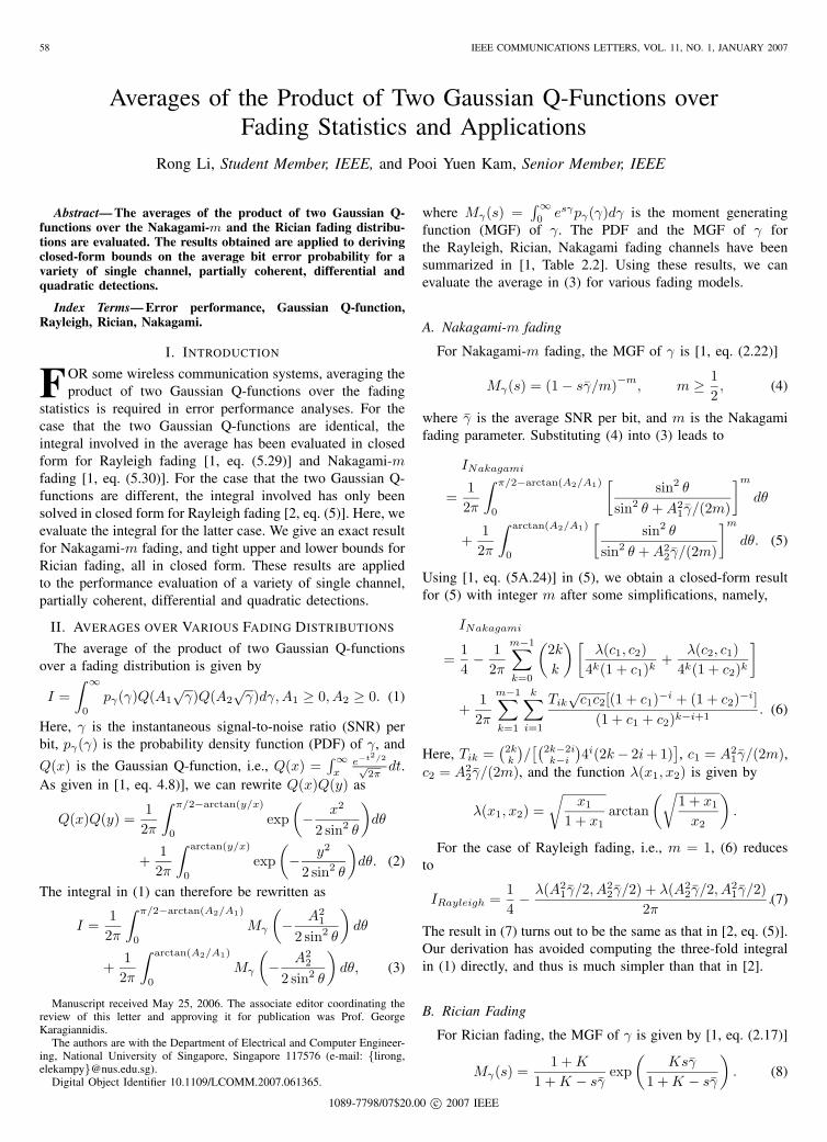
In (10), the equalities hold for K = 0 or η → ∞. The secondequality also holds for η = 0. Thus, the bounds on IRician in(11) and (12) equal the exact result in (9) when K = 0, i.e.,reduce to IRayleigh in (7). The upper bound is accurate whenr1 and r2 approach infinity or zero. The lower bound growstighter as r1 and/or r2 increase. Fig. 1 shows that at highSNR, both bounds converge to the exact value. For low SNRaround γ̄ = 0dB, the upper bound is close to the exact value,and much tighter than the lower bound. If γ̄ decreases further,the upper bound will merge with the exact value eventually.

III. BOUNDS ON THE AVERAGE BEP OF VARIOUS CASES

We now apply the results in Section II to performanceanalyses. The average bit error probability (BEP) over fadingchannels for a variety of single channel, partially coherent,differential and quadratic detections is given by [3, eq. (16)]

Pb =12

+12

∫ ∞

0

pγ(γ)[Q(a√

γ, b√

γ)−Q(b√

γ, a√

γ)]dγ,(13)

0 5 10 15 20 25 3010−9

10−8

10−7

10−6

10−5

10−4

10−3

10−2

10−1

Average SNR per Bit (dB)

I Ric

ian

ExactUpper boundLower bound

A1=6,A2=4,K=10

A1=1,A2=4,K=10

A1=1,A2=4,K=5

A1=1,A2=2,K=5

Fig. 1. Numerical results for IRician in (9) and its upper bound in (11)and lower bound in (12) versus γ̄.

where b > a ≥ 0, and Q(α, β) is the first-order MarcumQ-function. For Q(α, β) with α > 0 and β ≥ 0, we haveproposed an upper bound in [4, eq. (11)], i.e.,

Qerfc-UB1-KL(α, β)

= Q (β + α) + Q (β − α) +e−(β−α)2/2 − e−(β+α)2/2

α√

2π,(14)

and a lower bound in [4, eq. (12)], i.e.,

Qerfc-LB1-KL(α, β)= [Q (β + α) + Q (β − α)] [1 − 2Q (β)] + 2Q (β) . (15)

Our bounds in (14) and (15) are tighter than those in [3, eq.(3) and (4)] for most values of α and β [4]. Only for the casewhere α is close to zero and β is much larger than α is ourupper bound in (14) looser than that in [3, eq. (3)]. Using (14)and (15) to bound the Marcum Q-functions in (13), we obtaina new upper bound on Pb, i.e.,

Pb <12

+12

∫ ∞

0

pγ(γ) [Qerfc-UB1-KL(a√

γ, b√

γ)

− Qerfc-LB1-KL(b√

γ, a√

γ)] dγ

=∫ ∞

0

pγ(γ)

{Q((b − a)

√γ) +

12a

√2π

√γ

·{

exp[− (b − a)2γ

2

]− exp

[− (b + a)2γ

2

]}

+ [Q((b + a)√

γ) − Q((b − a)√

γ)]Q(a√

γ)

}dγ.(16)

In the following, we evaluate the right-hand side (RHS) of(16) first for Nakagami-m fading, and then for Rician fading.

For Nakagami-m fading, the PDF of γ is [1, eq. (2.21)]

pγ(γ) =mmγm−1

γ̄mΓ(m)exp

(−mγ

γ̄

), γ ≥ 0, (17)

where Γ(·) is the gamma function. For integer m, the RHS of(16) can be evaluated in closed form by using [1, eq. (5.18)],

60 IEEE COMMUNICATIONS LETTERS, VOL. 11, NO. 1, JANUARY 2007

0 5 10 15 20 25 3010−10

10−5

100

Average SNR per Bit (dB)(a) Nakagami −m fading

Ave

rage

Bit

Err

or P

roba

bilit

y P b

0 5 10 15 20 25 30

10−6

10−4

10−2

100

Average SNR per Bit (dB)(b) Rician fading

Ave

rage

Bit

Err

or P

roba

bilit

y P b

Exact in (13)

K=0

Upper bound in [3, eq. (18) ]

New upper bound in (18)

K=5

K=10

Exact in (13)

m=2

m=3m=4

New upper bound in (20)

Upper bound in [3, eq. (18) ]

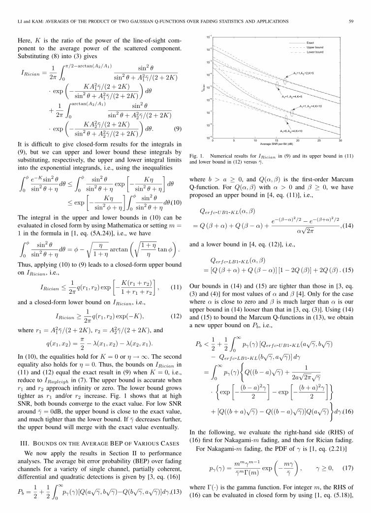
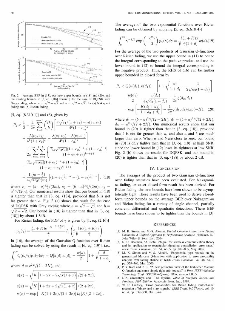
Fig. 2. Average BEP in (13), our new upper bounds in (18) and (20), andthe existing bounds in [3, eq. (18)] versus γ̄ for the case of DQPSK withGray coding, where a =

√2 −√

2 and b =√

2 +√

2, for (a) Nakagamifading and (b) Rician fading.

[5, eq. (8.310 1)] and (6), given by

Pb <12− 1

2π

m−1∑k=0

(2k

k

)[π√

e1/(1 + e1) − λ(e1, e3)4k(1 + e1)k

+λ(e2, e3)

4k(1 + e2)k+

λ(e3, e2) − λ(e3, e1)4k(1 + e3)k

]

+12π

m−1∑k=1

k∑i=1

{Tik

√e2e3[(1 + e2)−i + (1 + e3)−i]

(1 + e2 + e3)k−i+1

− Tik√

e1e3[(1 + e1)−i + (1 + e3)−i](1 + e1 + e3)k−i+1

}

+Γ(m − 1

2 )4√

πe3Γ(m)

[(1 + e1)

12−m − (1 + e2)

12−m

], (18)

where e1 = (b − a)2γ̄/(2m), e2 = (b + a)2γ̄/(2m), e3 =a2γ̄/(2m). Our numerical results show that our bound in (18)is tighter than that in [3, eq. (18)], provided that b is notfar greater than a. Fig. 2 (a) shows the result for the caseof DQPSK with Gray coding where a =

√2 −√

2 and b =√2 +

√2. Our bound in (18) is tighter than that in [3, eq.

(18)] by about 1.5dB.For Rician fading, the PDF of γ is given by [1, eq. (2.16)]

pγ(γ) =(1 + K)e−K− (1+K)γ

γ̄

γ̄I0

(2

√K(1 + K)γ

γ̄

).

In (16), the average of the Gaussian Q-function over Ricianfading can be solved by using the result in [6, eq. (19)], i.e.,∫ ∞

0

Q(c√

γ)pγ(γ)dγ = Q[u(d), v(d)] − w(d)2

[1 +

√d

1 + d

]

where d = c2γ̄/(2 + 2K), and

u(x) =√

K[1 + 2x − 2

√x(1 + x)

]/(2 + 2x),

v(x) =√

K[1 + 2x + 2

√x(1 + x)

]/(2 + 2x),

w(x) = exp [−K(1 + 2x)/(2 + 2x)] I0 [K/(2 + 2x)] .

The average of the two exponential functions over Ricianfading can be obtained by applying [5, eq. (6.618 4)]

∫ ∞

0

γ−1/2 exp(−c2γ

2

)pγ(γ)dγ =

√(1 + K)πγ̄(1 + d)

w(d).(19)

For the average of the two products of Gaussian Q-functionsover Rician fading, we use the upper bound in (11) to boundthe integral corresponding to the positive product and use thelower bound in (12) to bound the integral corresponding tothe negative product. Thus, the RHS of (16) can be furtherupper bounded in closed form by

Pb < Q(u(d1), v(d1)) −[1 +

√d1

1 + d1− 1

2√

d3(1 + d1)

]

· w(d1)2

− w(d2)4√

d3(1 + d2)+

12π

q(d2, d3)

· exp[−K(d2 + d3)

1 + d2 + d3

]− 1

2πq(d1, d3) exp(−K), (20)

where d1 = (b − a)2γ̄/(2 + 2K), d2 = (b + a)2γ̄/(2 + 2K),d3 = a2γ̄/(2 + 2K). Our numerical results show that ourbound in (20) is tighter than that in [3, eq. (18)], providedthat b is not far greater than a, and also a and b are muchlarger than zero. When a and b are close to zero, our boundin (20) is only tighter than that in [3, eq. (18)] at high SNR,since the lower bound in (12) loses its tightness at low SNR.Fig. 2 (b) shows the results for DQPSK, and our bound in(20) is tighter than that in [3, eq. (18)] by about 2 dB.

IV. CONCLUSION

The averages of the product of two Gaussian Q-functionsover fading statistics have been evaluated. For Nakagami-m fading, an exact closed-form result has been derived. ForRician fading, the new bounds have been shown to be asymp-totically tight. These results have been used to derive closed-form upper bounds on the average BEP over Nakagami-mand Rician fading for a variety of single channel, partiallycoherent, differential and quadratic detections. These BEPbounds have been shown to be tighter than the bounds in [3].

REFERENCES

[1] M. K. Simon and M.-S. Alouini, Digital Communication over FadingChannels: A Unified Approach to Performance Analysis. Hoboken, NJ:John Wiley & Sons, Inc., 2004.

[2] N. C. Beaulieu, “A useful integral for wireless communication theoryand its application to rectangular signaling constellation error rates,”IEEE Trans. Commun., vol. 54, no. 5, pp. 802–805, May 2006.

[3] M. K. Simon and M.-S. Alouini, “Exponential-type bounds on thegeneralized Marcum Q-function with application to error probabilityanalysis over fading channels,” IEEE Trans. Commun., vol. 48, no. 3,pp. 359–366, Mar. 2000.

[4] P. Y. Kam and R. Li, “A new geometric view of the first-order MarcumQ-function and some simple tight erfc-bounds,” in Proc. IEEE VehicularTechnology Conf. (VTC2006-Spring) 2006, session 11G.5.

[5] I. S. Gradshteyn and I. M. Ryzhik, Table of Integrals, Series, andProducts, Fifth Edition. Academic Press, Inc., 1994.

[6] W. C. Lindsey, “Error probabilities for Rician fading multichannelreception of binary and n-ary signals,” IEEE Trans. Inf. Theory, vol. 10,no. 4, pp. 339–350, Oct. 1964.