Embed Size (px)
Citation preview

i
Availability Estimation and Management
for Complex Processing Systems
By
Qadeer Ahmed
A thesis submitted to the School of Graduate Studies
in partial fulfillment of the requirements for the degree of
Doctor of Philosophy
Faculty of Engineering and Applied Science
Memorial University of Newfoundland
May - 2016
St. John’s, Newfoundland
ii
Abstract
“Availability” is the terminology used in asset intensive industries such as
petrochemical and hydrocarbons processing to describe the readiness of equipment, systems
or plants to perform their designed functions. It is a measure to suggest a facility’s capability
of meeting targeted production in a safe working environment. Availability is also vital as it
encompasses reliability and maintainability, allowing engineers to manage and operate
facilities by focusing on one performance indicator. These benefits make availability a very
demanding and highly desired area of interest and research for both industry and academia.
In this dissertation, new models, approaches and algorithms have been explored to
estimate and manage the availability of complex hydrocarbon processing systems. The risk of
equipment failure and its effect on availability is vital in the hydrocarbon industry, and is also
explored in this research. The importance of availability encouraged companies to invest in
this domain by putting efforts and resources to develop novel techniques for system availability
enhancement. Most of the work in this area is focused on individual equipment compared to
facility or system level availability assessment and management. This research is focused on
developing an new systematic methods to estimate system availability. The main focus areas
in this research are to address availability estimation and management through physical asset
management, risk-based availability estimation strategies, availability and safety using a
iii
failure assessment framework, and availability enhancement using early equipment fault
detection and maintenance scheduling optimization.
Keywords: Asset Management, Availability, Reliability, Maintainability, Safety, Risk
Assessment, Root Cause Analysis, Fault Detection, Decision Trees, Maintenance Scheduling
Optimization, Markov Decision Process, Genetic Algorithms

iv
To my parents…
To my family, friends …
and
To my wife and kids…

v
Acknowledgments
All praises are due to almighty Allah, who has given us the opportunity and strength to
complete this work. It is my pleasure to acknowledge several individuals for their guidance,
contribution and support throughout my Ph.D. program.
First and foremost, I would like to offer my sincere thanks to my main supervisor, Dr.
Faisal Khan, for all his support, guidance and encouragement throughout the program. Without
his support and guidance, it would not have been possible to meet the research requirements
of this Ph.D. work. I am also very thankful to my co-supervisors, Dr. Yan Zhang, Dr. Salim
Ahmed and Dr. Syed A. Raza for their valuable guidance and support throughout this program.
I would like to offer thanks to my research colleagues Dr. Syed Asif Raza, Dr. Kamran
Moghaddam and Dr. Fatai Adesina Anifowose for their contributions and support to develop
some novel and outstanding solutions to address industry problems. I would like to extend
sincere thanks to examination committee members, Dr. Ming Zuo, Dr. Syed Ahmed Imtiaz,
and Dr. Long Fan for providing valuable feedback to improve the overall quality of the thesis.
Along the way, several people have helped me in different ways to achieve my goal. I would
to like to thank Mr. Khalid B. Hanif, Mr. Subba R. Ganti, Mr. Samith Rathnayaka and Dr.
Refaul Ferdous for their help and support.

vi
I am indebted to the graduate studies department of Memorial University for providing
me with such a great opportunity. I am sincerely thankful to all who helped me, including the
administrative, technical and academic staff at Memorial University.
Last but not least, I would like to thank my parents and family for their prayers and
unselfish support in helping me to grow as a person and in securing for me an outstanding
education. I take this opportunity to express my deep and heart-felt gratitude to my wife,
Farida, for making great efforts to manage the family, which indeed enabled me to complete
these studies. I also would like to express my thanks to my beloved children, Momena, Sarah,
Ibrahim and Aamna for their understanding, patience and sacrifices during my studies.

vii
Co-Authorship Statement
I, Qadeer Ahmed, hold a primary author status for all the Chapters in this dissertation.
However, each manuscript is co-authored by my supervisor, co-researchers and colleagues,
whose contributions have facilitated the development of this work as described below.
Qadeer Ahmed, Faisal I. Khan, Syed A. Raza, (2014) "A risk-based availability
estimation using Markov method," International Journal of Quality & Reliability
Management, Vol. 31 Issue: 2, pp.106-128.
Statement: I am the primary author and carried out most of the data collection,
numerical modeling and analysis. I have drafted the manuscript and included all the
comments after review from co-authors in the final manuscript. As co-author, Faisal I.
Khan helped in developing the idea, reviewed, corrected the model and results. He also
contributed in reviewing and revising the manuscript. As co-author, Syed A. Raza
contributed through support in development of state dependent models along with
reviewing and revising the manuscript.
Qadeer Ahmed, Faisal Khan, Salim Ahmed, (2014), “Improving safety and
availability of complex systems using a risk-based failure assessment approach,”
Journal of Loss Prevention in the Process Industries, Volume 32, November 2014,
pp. 218-229.

viii
Statement: In primary author capacity, I was involved in data collection and analysis,
development of framework, implementation of framework for validation of the
proposed framework and compilation of results. I have drafted the manuscript for
review and comments, later, included all the comments from co-authors in the final
manuscript. As co-author, Faisal I. Khan identified the improvements required for
overall framework to be more practical and realistic. He supported in finalizing the
methodology to implement the framework. He also contributed in reviewing and
revising the manuscript. As co-author, Salim Ahmed contributed through support in
development of case studies to validate the proposed framework along with reviewing
and revising the manuscript.
Qadeer Ahmed, Kamran S. Moghaddam, Syed A. Raza, Faisal I. Khan, (2015),
“A Multi Constrained Maintenance Scheduling Optimization Model for
Hydrocarbon Processing Facilities,” Proceedings of the Institution of Mechanical
Engineers, Part O: Journal of Risk and Reliability, pp 151-168
Statement: As a primary author, I was involved in development of the cost, reliability
and availability optimization models. I carried out the data collection, analysis using
the optimization code for all the optimization cases and formulation of results. I have
drafted the manuscript for review and comments, later, included all the comments from
co-authors in the final manuscript. As a co-author, Kamran S. Moghaddam contributed
in coding the proposed optimization formulation and ensured its working in

ix
optimization software, LINGO. He also contributed in reviewing and revising the
manuscript. As co-author, Syed A. Raza supported in development of optimization
formulation, especially development of failure model. Faisal I. Khan supported in
developing the idea, reviewed, and provided comments to ensure models are
representative of real plant conditions which includes maintenance cost, reliability and
availability. He contributed in reviewing the draft manuscript and provided comments
to improve the manuscript.
Qadeer Ahmed, Fatai A. Anifowose, Faisal Khan, (2015), “System Availability
Enhancement using Computational Intelligence based Decision Tree Predictive
Model,” Accepted - Proceedings of the Institution of Mechanical Engineers, Part
O: Journal of Risk and Reliability
Statement: I am the primary author developed the concept of early fault detection to
enhance system availability. I also carried out the data collection and analysis,
development of fault detection schemes, designed experiments to include all the
operating conditions. I have performed all the cases model execution using MATLAB
and compilation of results. I have drafted the manuscript for review and comments,
later, included all the comments from co-authors in the final manuscript. As a co-
author, Fatai A. Anifowose participated in development the code and data stratification
strategy in MATLAB using Decision Trees algorithms. He also contributed in
reviewing and revising the manuscript. As co-author, Faisal Khan contributed in
x
developing the idea to detect machinery faults, reviewed, and feedback on the model
and results. He also contributed in reviewing and suggesting areas to improve the
manuscript.
Abdel Kader Attou and Qadeer Ahmed, (2009), "Asset Management Practices at
Qatargas," Proceedings of the 1st Annual Gas Processing Symposium, Doha,
Qatar. Elsevier B.V.
Statement: I am the primary author in this paper and presented the importance of
physical asset management in enhancing availability of assets. I have drafted the
manuscript for review and comments, later, included all the comments from co-authors
in the final manuscript. As a co-author, Abdel Kader Attou has contributed by
reviewing the concept and its refinement. He suggested practical improvements based
on his extensive experience in industry and supported the proposed asset management
concept. He also reviewed the results and suggested changes in manuscript to enhance
the quality of the paper.
Qadeer Ahmed

xi
Table of Contents
Abstract ..................................................................................................................................... ii
Acknowledgments..................................................................................................................... v
Co-Authorship Statement........................................................................................................ vii
Table of Contents ..................................................................................................................... xi
List of Figures ......................................................................................................................... xv
List of Tables ........................................................................................................................ xvii
List of Symbols & Abbreviations .......................................................................................... xix
CHAPTER 1 ............................................................................................................................. 1
INTRODUCTION AND OVERVIEW .................................................................................... 1
1.1 Introduction .................................................................................................................... 1
1.2 Research Objective and Scope ....................................................................................... 3
1.3 General Terminology and Definitions ........................................................................... 5
1.4 Literature Survey ......................................................................................................... 15
1.5 Constraints and Limitations ......................................................................................... 27
1.6 Thesis Structure ........................................................................................................... 29
CHAPTER 2 ........................................................................................................................... 31

xii
RISK-BASED AVAILABILITY ESTIMATION USING A MARKOV MODEL .............. 31
Abstract ................................................................................................................................... 31
2.1 Introduction .................................................................................................................. 33
2.2 Risk and Risk Assessment ........................................................................................... 40
2.3 Risk-based Availability Modeling Framework ............................................................ 44
2.4 Application of Proposed Methodology ........................................................................ 50
2.5 Numerical Analysis and Results .................................................................................. 62
2.6 Conclusion ................................................................................................................... 67
CHAPTER 3 ........................................................................................................................... 69
IMPROVING AVAILABILITY USING A RISK-BASED FAILURE ASSESSMENT
APPROACH .......................................................................................................................... 69
Abstract ................................................................................................................................... 69
3.1 Introduction .................................................................................................................. 70
3.2 Background Study ........................................................................................................ 74
3.3 Risk-Based Failure Assessment (RBFA) Framework ................................................. 78
3.4 Application of Proposed Approach using Case Studies .............................................. 89
3.5 Critical Success Factors – RBFA Methodology ........................................................ 102
3.6 Conclusion ................................................................................................................. 103

xiii
CHAPTER 4 ......................................................................................................................... 105
SYSTEM AVAILABILITY ENHANCEMENT USING DECISION TREES ................... 105
Abstract ................................................................................................................................. 105
4.1 Introduction ................................................................................................................ 106
4.2 Literature Review....................................................................................................... 112
4.3 Proposed Fault Detection and Management Framework ........................................... 115
4.4 Experimental Setup and Data Collection ................................................................... 124
4.5 Results and Discussion .............................................................................................. 130
4.6 Conclusion ................................................................................................................. 137
CHAPTER 5 ......................................................................................................................... 140
A MULTI-CONSTRAINED MAINTENANCE SCHEDULING OPTIMIZATION ......... 140
Abstract ................................................................................................................................. 140
5.1 Introduction ................................................................................................................ 141
5.2 Literature Research .................................................................................................... 150
5.3 Formulation of a Maintenance Optimization Model ................................................. 156
5.4 Optimization Models ................................................................................................. 171
5.5 Data and Computational Results Summary ............................................................... 176
5.6 Conclusion ................................................................................................................. 187
xiv
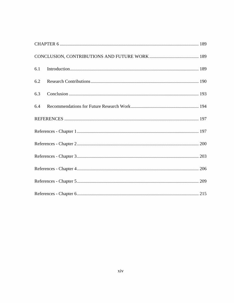
CHAPTER 6 ......................................................................................................................... 189
CONCLUSION, CONTRIBUTIONS AND FUTURE WORK ........................................... 189
6.1 Introduction ................................................................................................................ 189
6.2 Research Contributions .............................................................................................. 190
6.3 Conclusion ................................................................................................................. 193
6.4 Recommendations for Future Research Work ........................................................... 194
REFERENCES ..................................................................................................................... 197
References - Chapter 1 .......................................................................................................... 197
References - Chapter 2 .......................................................................................................... 200
References - Chapter 3 .......................................................................................................... 203
References - Chapter 4 .......................................................................................................... 206
References - Chapter 5 .......................................................................................................... 209
References - Chapter 6 .......................................................................................................... 215
xv
List of Figures
Figure 1.1: Overall research strategy ........................................................................................ 4
Figure 1.2: Repairable system................................................................................................. 11
Figure 1.3: Non repairable system .......................................................................................... 12
Figure 2.1: Asset Centric Approach ........................................................................................ 18
Figure 2.2: General strategy – five key steps .......................................................................... 20
Figure 2.2: Risk assessment matrix ........................................................................................ 42
Figure 2.3: Flow diagram of risk based availability model .................................................... 47
Figure 2.5: Functional block diagram ..................................................................................... 55
Figure 2.6: State diagram of two pieces of equipment in parallel with failure in standby ..... 60
Figure 2.7: State diagram of a three state degraded system with repair ................................. 61
Figure 2.8: Graphical comparison of availabilities ................................................................. 65
Figure 3.1: Availability – operate and maintain ..................................................................... 76
Figure 3.2: Four phases – risk-based failure assessment ........................................................ 80
Figure 3.3: Proposed RCFA framework ................................................................................. 82
Figure 3.4: Risk assessment matrix ........................................................................................ 83
Figure 3.5: Prioritization matrix for corrective actions .......................................................... 88
Figure 3.6: Pumping system ................................................................................................... 90
Figure 3.7: Failure event timeline ........................................................................................... 91
Figure 3.8: Failure cause relationship tree .............................................................................. 92
Figure 3.9: Evidence – failed part condition ........................................................................... 93

xvi
Figure 3.10: Vibration Trend – overall vibration and bearing frequency ............................... 93
Figure 3.11: Simple supply system configuration .................................................................. 97
Figure 3.12: Coupling and bearing failure .............................................................................. 98
Figure 3.13: Pump misalignment condition ............................................................................ 99
Figure 4.1: Diagnostic-prognostic concept with equipment condition, risk and cost ........... 109
Figure 4.2: Spectrum snapshot of misalignment and unbalance ........................................... 110
Figure 4.3: Fault detection and management framework ..................................................... 117
Figure 4.4: Experimental setup in a laboratory ..................................................................... 125
Figure 4.5: Waterfall plot for Unbalance under three different unbalance conditions ......... 128
Figure 4.6: Snap Shot of Bode Plots with 2.2 grams of Unbalance ..................................... 128
Figure 4.7: Effect of features on classification accuracy ...................................................... 132
Figure 4.8: Classification accuracies — stratification levels and algorithms ...................... 134
Figure 4.9: Classification accuracy comparison ................................................................... 136
Figure 5.1: General product flow in a gas processing plant [4] ............................................ 147
Figure 5.2: Maintenance types in a time period .................................................................... 162
Figure 5.3: Conceptual effect on reliability under different maintenance tasks ................... 165
Figure 5.4: Overall Schematic of a Gas Absorption System [4] ........................................... 172

xvii
List of Tables
Table 2.1: Safety Health and Environment ............................................................................. 53
Table 2.2: Economics, Reliability and Maintainability .......................................................... 54
Table 2.3: Rotating Equipment ............................................................................................... 57
Table 2.4: Static Equipment .................................................................................................... 58
Table 2.5: Individual Availabilities of Subsystems ................................................................ 63
Table 3.1: Failure and Repair Data of Pumping System ........................................................ 94
Table 3.2: Results – Availability Improvement ...................................................................... 95
Table 3.3: Failure and Repair Data of a Pumping System .................................................... 101
Table 3.4: Results – Availability Estimation ........................................................................ 102
Table 4.1: Fault Management Matrix ................................................................................... 123
Table 4.2: Experimental Setup for the Laboratory Test ....................................................... 126
Table 4.3: Data Collection Strategy for the Test .................................................................. 126
Table 4.4: Equipment Simulator Descriptive Data Statistics................................................ 129
Table 4.5: Real Plant Descriptive Data Statistics ................................................................. 129
Table 4.6: Fault Classification Accuracy using Gini Index Split ......................................... 131
Table 4.7: Fault Classification Accuracy using Twoing Split .............................................. 131
Table 4.8: Fault Classification Accuracy using Deviance Split .......................................... 131
Table 4.9: Effect of the Number of Features on Average Classification Accuracy ............. 132
Table 4.10: Test Results after Data Cleanup at 70% Stratification ...................................... 134
Table 4.11: Real Plant Equipment Data Results ................................................................... 135

xviii
Table 5.1: Maintenance Task Cost Data ............................................................................... 176
Table 5.2: Maintenance Task Duration and Reliability Data ............................................... 177
Table 5.3: Existing Maintenance Cost .................................................................................. 179
Table 5.4: Existing Maintenance Schedule for Gas Absorption System ............................. 179
Table 5.5: Gas Absorption System – Availability and Reliability........................................ 181
Table 5.6: Total Maintenance Cost Subject to Reliability Constraints ................................. 182
Table 5.7: Total Maintenance Cost Subject to Reliability Constraints ................................. 182
Table 5.8: Effect of ERI on the Maintenance Schedule ........................................................ 183
Table 5.9: Maximize Reliability Subject to Availability Constraint .................................... 184
Table 5.10: Maximize Reliability Subject to Availability Constraint .................................. 184
Table 5.11: Goals and Weights for Goal Programming ....................................................... 185
Table 5.12: Schedule – Weights for Cost: 0.5, Reliability: 0.4, and Availability: 0.1 ......... 186
Table 5.13: Schedule – Weights for Cost: 0.3, Reliability: 0.6 and Availability: 0.1 .......... 186
Table 5.14: Summary of Results – Goal Programming ........................................................ 187

xix
List of Symbols & Abbreviations
Symbol/
Abbreviation
Description
Atarget Required Availability of a Complete System
CFm Cost of Corrective (failure) Task of Equipment, m
CIm Cost of Inspection of Equipment, m
CLFm Labor Cost/hour to Perform a Corrective Task for Equipment, m
CLIm Labor Cost/hour to Perform an Inspection Task for Equipment, m
CLMm Labor Cost/hour to Perform a Maintenance Task for Equipment, m
CLRm Labor Cost/hour to Perform a Replacement Task for Equipment, m
CMm Cost of Maintenance of Equipment, m
CMTm Cost of the Material of Equipment, m
COm Cost of Operation Task of Equipment, m
CRm Cost of Replacement of Components in Equipment, m
E[Nmt] Expected Number of Failures of Equipment, m, and Time, t
ERIm Equipment Risk Index of Equipment, m
Rtarget Required Reliability of a Complete System
TFm Time Required to Perform a Corrective Repair for Equipment, m
TIm Time Required to Inspect Equipment, m
TMm Time Required to Perform Maintenance on Equipment, m

xx
TRm Time Required to Replacement Equipment, m
αm Improvement Factor of Equipment, m
βm Shape Parameter of Equipment, m
λm Scale Parameter of Equipment, m
νm Rate of Occurrence of Failure (ROCOF)
ρm Failure Cost Factor for Equipment, m
A Availability
ACA Asset Centric Approach
ALARP As Low As Reasonably Possible
AM Asset Management
AMMS Asset Maintenance Management System
API American Petroleum Institute
APMS Asset Performance Management System
AS System Availability
AsR Availability – System Rotating Equipment
Ass Availability – System Static Equipment
AU Availability – Unit
DT Decision Trees
FDC Fault Detection and Control
FTA Fault Tree Analysis
HP High Pressure

xxi
ISO International Standard Organization
ISO International Standard Organization
L Length of the Planning Horizon
LB Lower Bound
LP Low Pressure
M Maintainability
M Number of Equipment
M Index for an Equipment, ∀ m = {1,2,3, … , M}
M’
MTBF
Mean System Downtime
Mean Time Between Failure
MDP Markov Decision Process
MM Markov Modeling
MTBF Mean Time Between Failures
MTBM
RBD
Mean Time between Maintenance
Reliability Block Diagram
MTTR Mean Time to Repair
OREDA Offshore Reliability Data
PAM Physical Asset Management
PERD Process Equipment Reliability Database
PI Priority Index
POF Probability of Failure

xxii
QLRA Qualitative Risk Assessment
QNRA Quantitative Risk Assessment
R Reliability
RA Risk Assessment
RAM Risk Assessment Matrix
RBAMM Risk Based Availability Markov Model
RBD Reliability Block Diagram
RI Risk Index
ROA Return on Investment
Rp Reliability of Parallel System
Rs Reliability of Series System
SHE Safety, Health, and Environment
SR System Rotating Equipment
SRn Subsystem in Rotating Equipment
SS System Static Equipment
SSn Subsystem in Static Equipment
T Number of Intervals over the Planning Horizon
T Index for Time Period, ∀ t = {1,2,3, … , T}
TC Total Cost
UB Upper Bound
UKF Unscented Kalman Filter

xxiii
λm Failure Rate
µ Repair Rate
1
CHAPTER 1
INTRODUCTION AND OVERVIEW
1.1 Introduction
High availability means effective utilization and management of equipment,
processes and other resources. This helps to improve the return on investment for all
stakeholders by ensuring the facilities produce to meet required demand. Availability is a
function of reliability and maintainability; therefore, availability is an important measure
in the processing industry. Over the last decade, there has been an increasing trend of
companies integrating processes and utilizing excess available capacities in other places to
achieve economies of scale and improve plant availability. The overall availability
management process requires many systems working concurrently to reap the real benefits.
This requires multiple departments to work together such as Maintenance and Operations;
and many systems to be aligned toward a common goal, along with continuous monitoring
and improvement for sustainability.
There are many general methods to calculate the availability of systems and
equipment. Different methods are used to estimate the availability of a product or a process.

2
Availability of processes has reliability and maintainability aspects embedded in the
analysis, which makes it a powerful mechanism to manage businesses. Processing systems
comprise different equipment with redundancies; for example, a liquefaction system
converts gas into liquid by cooling and processing the gas through many compressors,
turbines, vessels and valves. Estimation and management of availability in a complex
operating facility is a challenging task, requiring the use of modern tools, engineering
algorithms and engineering experience. In this research, we have developed some novel
techniques to address availability using Markov-based state dependent models, risk based
strategies, fault detection and its management along with maintenance scheduling
optimization.
This dissertation is organized based on the above-mentioned focus areas. Chapter
1 is focused on introduction and overview of availability estimation and management.
Some basic availability, risk and reliability concepts and definitions are also discussed in
this chapter. The concept of PAM is vital and a foundation to the overall Availability
Management (AM) process. AM mainly comprises two main components; one is asset
maintenance management and the other is asset performance management is also part of
this Chapter. In Chapter 2, a risk-based stochastic modeling approach based on the Markov
Decision Process (MDP) is discussed to estimate availability of a plant. A model is
developed based on critical equipment of a system to estimate overall processing unit
availability. The developed model is applied on a gas absorption process to ensure its
application on real-world problems. Chapter 3 describes a novel risk-based failure
assessment approach to address the safety and availability of complex operating systems.

3
A structured process is proposed and validated using real-world failure assessment cases
to prove the applicability and efficacy of the proposed model.
In the next Chapter, early fault detection and management is explained to support
availability and safety improvement. Decision Trees (DTs) are introduced as a predictive
data mining tool to detect early faults and their management to improve system availability.
To conclude the effectiveness of the model, the proposed model was successfully tested to
detect faults using real plant machinery vibration data. As discussed earlier, maintainability
is important in availability management and so maintenance and its optimization is
considered in this research. In Chapters 5, multi-constrained, multi-objective maintenance
scheduling optimization models are proposed. The optimization problem was developed
considering the time-dependent equipment failure rate to optimize maintenance costs at
different availability and reliability levels. These models were applied on a plant scenario
to show the effectiveness of maintenance scheduling optimization on cost, availability and
reliability.
Finally, Chapter 6 concludes the research with the key findings, contributions and
suggests possible expansion ideas for this work.
1.2 Research Objective and Scope
Availability is an extremely important parameter to ensure the continuous operation
of facilities. Due to its importance and usefulness in asset intensive industries, we focused
on developing comprehensive methods and models for availability estimation and

4
management. These new methodologies and models mainly help to address the critical
issues of unwanted breakdowns in processing facilities. These breakdowns have severe
financial consequences along with adverse health, safety and environment consequences.
There are many ways to estimate and improve availability, as presented in the next
Chapters. We proposed some new models and algorithms, which can help improve and
manage the availability of a complex processing facility. Generally, processing facilities
lose millions of dollars in lost production due to unwanted breakdowns or interruptions,
this research effort is a great resource to minimize such losses by properly utilizing these
developments.
Figure 1.1: Overall research strategy
The specific objectives of this research are to develop effective and novel
availability estimation and management methodologies for complex processing systems.
Availability Estimation and Management
Availability using
maintenance optimization
Physical Asset Management
Risk -based estimation
using Markov
Risk-based failure
assessment frameork
Early fault detection and management

5
This research objective is realized by working on the following areas as presented in Figure
1.1.
a. Developed a physical asset management model and integrate for
availability.
b. Developed a state dependent risk-based availability estimation method
using the Markov method.
c. Developed a risk-based failure assessment framework to address safety and
availability.
d. Developed model for early fault detection and management to enhance
availability.
e. Developed multi-objective maintenance scheduling optimization models to
enhance availability and reliability goals.
1.3 General Terminology and Definitions
To better understand the concepts in this dissertation, basic definition and
terminology is discussed below.
1.3.1 Operational Measures
Many different measures are being used in the industry to monitor the efficiency
and effectiveness of the processes, equipment and maintenance. Some of the key measures
are defined below:

6
1.3.1.1 Availability
Availability is to identify if the equipment or process is available at a given time
to perform its intended function. Availability is a function of reliability and maintainability.
There are many types of availabilities in literature so it is important to understand them to
use them properly. Availability can be defined as,
“Ability of an item to be in a state to perform a required function under given
conditions at a given instant of time or during a given interval, assuming that the required
external resources are provided” [1].
Other definition of availability,
“It is probability that a system or component is performing its required function at
a given point in time or over a stated period of time when operated and maintained in a
prescribed manner” [2].
Availability is also a probability like reliability and maintainability. Availability,
sometimes referred as Inherent or average availability is measured as,
𝐴 =𝑈𝑝𝑡𝑖𝑚𝑒
𝑈𝑝𝑡𝑖𝑚𝑒 + 𝐷𝑜𝑤𝑛𝑡𝑖𝑚𝑒 (1.1)
𝐴 =𝑀𝑇𝐵𝐹
𝑀𝑇𝐵𝐹 + 𝑀𝑇𝑇𝑅
(1.2)
Where MTBF – Mean Time between Failure
MTTR – Mean Time to Repair

7
The other forms of steady state availability depend on the definition of uptime and
downtime, the brief discussion about them follows:
1.3.1.1.1 Achieved Availability
Achieved availability is defined as,
𝐴𝑎 =𝑀𝑇𝐵𝑀
𝑀𝑇𝐵𝑀 + 𝑀′ (1.3)
Where, 𝑀′= Mean System Downtime, 𝑀𝑇𝐵𝑀 = Mean Time Between Maintenance
In this form, 𝑀′ is the mean system downtime and 𝑀𝑇𝐵𝑀 includes both
unscheduled and preventive maintenance and is computed as,
𝑀𝑇𝐵𝑀 = 𝑡𝑑
𝑚𝑡𝑑 +𝑡𝑑
𝑇𝑝𝑚⁄
(1.4)
Where, 𝑡𝑑= Unscheduled Downtime, 𝑇𝑝𝑚 = Preventive Maintenance Time
1.3.1.1.2 Operational Availability
Operational availability is defined as,
𝐴𝑎 =𝑀𝑇𝐵𝑀
𝑀𝑇𝐵𝑀 + 𝑀′′ (1.5)
Where 𝑀′′ is determined by replacing MTTR with MTR. MTR is calculated using equation
below,
𝑀𝑇𝑅 = 𝑀𝑇𝑇𝑅 + 𝑆𝐷𝑇 + 𝑀𝐷𝑇 (1.6)
Where, 𝑀𝑇𝑅 = Mean Repair Time, 𝑆𝐷𝑇 = Schedule Downtime
8
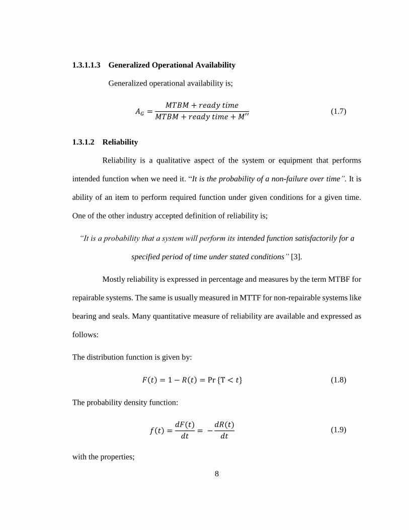
1.3.1.1.3 Generalized Operational Availability
Generalized operational availability is;
𝐴𝐺 =𝑀𝑇𝐵𝑀 + 𝑟𝑒𝑎𝑑𝑦 𝑡𝑖𝑚𝑒
𝑀𝑇𝐵𝑀 + 𝑟𝑒𝑎𝑑𝑦 𝑡𝑖𝑚𝑒 + 𝑀′′ (1.7)
1.3.1.2 Reliability
Reliability is a qualitative aspect of the system or equipment that performs
intended function when we need it. “It is the probability of a non-failure over time”. It is
ability of an item to perform required function under given conditions for a given time.
One of the other industry accepted definition of reliability is;
“It is a probability that a system will perform its intended function satisfactorily for a
specified period of time under stated conditions” [3].
Mostly reliability is expressed in percentage and measures by the term MTBF for
repairable systems. The same is usually measured in MTTF for non-repairable systems like
bearing and seals. Many quantitative measure of reliability are available and expressed as
follows:
The distribution function is given by:
𝐹(𝑡) = 1 − 𝑅(𝑡) = Pr {T < 𝑡} (1.8)
The probability density function:
𝑓(𝑡) =𝑑𝐹(𝑡)
𝑑𝑡= −
𝑑𝑅(𝑡)
𝑑𝑡 (1.9)
with the properties;
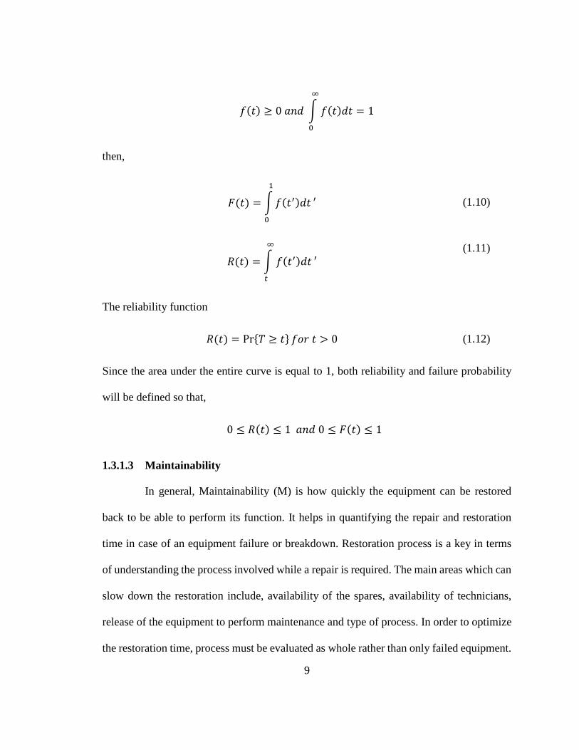
9
𝑓(𝑡) ≥ 0 𝑎𝑛𝑑 ∫ 𝑓(𝑡)𝑑𝑡
∞
0
= 1
then,
𝐹(𝑡) = ∫ 𝑓(𝑡′)𝑑𝑡
1
0
′ (1.10)
𝑅(𝑡) = ∫ 𝑓(𝑡′)𝑑𝑡
∞
𝑡
′ (1.11)
The reliability function
𝑅(𝑡) = Pr{𝑇 ≥ 𝑡} 𝑓𝑜𝑟 𝑡 > 0 (1.12)
Since the area under the entire curve is equal to 1, both reliability and failure probability
will be defined so that,
0 ≤ 𝑅(𝑡) ≤ 1 𝑎𝑛𝑑 0 ≤ 𝐹(𝑡) ≤ 1
1.3.1.3 Maintainability
In general, Maintainability (M) is how quickly the equipment can be restored
back to be able to perform its function. It helps in quantifying the repair and restoration
time in case of an equipment failure or breakdown. Restoration process is a key in terms
of understanding the process involved while a repair is required. The main areas which can
slow down the restoration include, availability of the spares, availability of technicians,
release of the equipment to perform maintenance and type of process. In order to optimize
the restoration time, process must be evaluated as whole rather than only failed equipment.

10
The parameter using by the industry to measure the maintainability is MTTR. As per
industry accepted standards,
“Ability of an item under given conditions of use, to be retained in, or restored to, a state
in which it can perform a required function, when maintenance is performed under given
conditions and using stated procedures and resources”[1].
1.3.1.4 Utilization
Utilization is simply a ratio between the actual produced compared to planned
production. This ratio gives us an idea how well we are performing compared to the
planned or sometime called nameplate capacity.
Mathematically can be written as Equation 1.13,
𝑈𝑡𝑖𝑙𝑖𝑧𝑎𝑡𝑖𝑜𝑛 =𝐴𝑐𝑡𝑢𝑎𝑙 𝑃𝑟𝑜𝑑𝑢𝑐𝑡𝑖𝑜𝑛
𝑃𝑙𝑎𝑛𝑛𝑒𝑑 𝑃𝑟𝑜𝑑𝑢𝑐𝑡𝑖𝑜𝑛 (1.13)
1.3.1.5 System Categorization
There are two types of system, repairable and non-repairable. When a system fails
to perform its intended function, this state usually termed as non-functional and denoted
by state 0. The other scenario is vice versa and that is when the system is working as
intended and represented by state 1. If a system can be brought back from a failed sate to a
functional state, the system categorizes as repairable system like compressor, pumps, and
mechanical seals. In other condition, if the system cannot bring back into its functional
state after failing the system is categorized as non-repairable systems, for example,
bearings and gaskets.
11
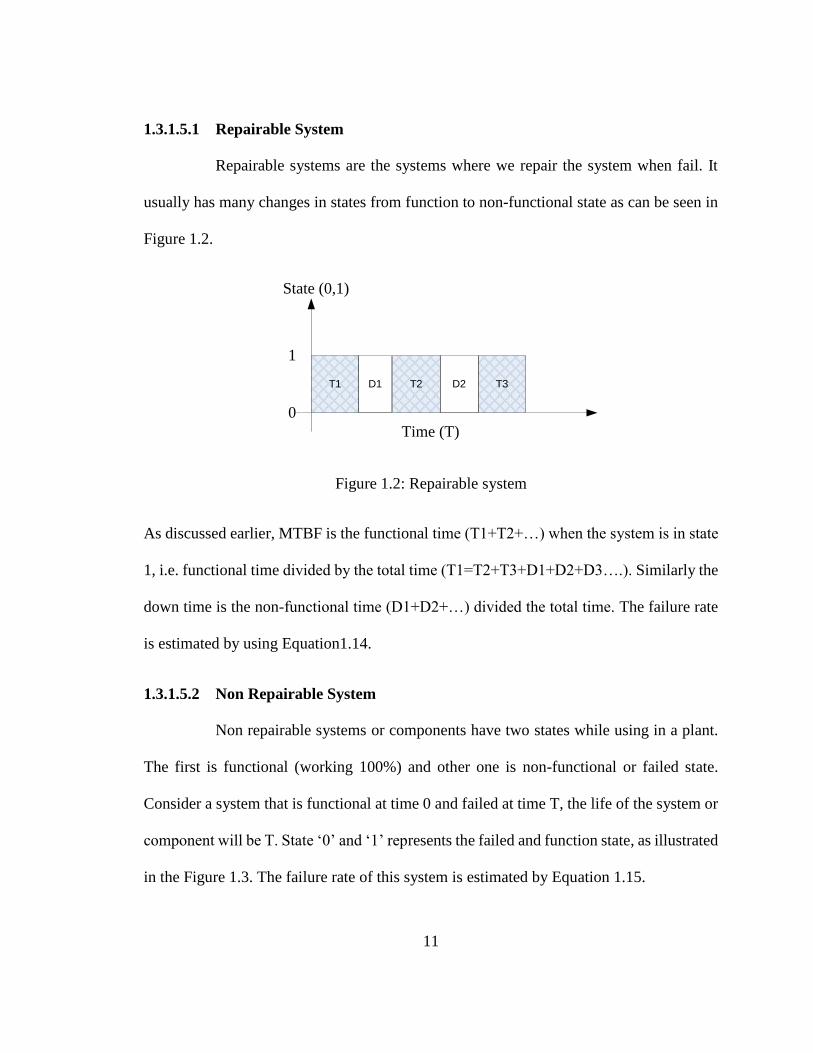
1.3.1.5.1 Repairable System
Repairable systems are the systems where we repair the system when fail. It
usually has many changes in states from function to non-functional state as can be seen in
Figure 1.2.
Time (T)
State (0,1)
0
1
T1 T2 T3D1 D2
Figure 1.2: Repairable system
As discussed earlier, MTBF is the functional time (T1+T2+…) when the system is in state
1, i.e. functional time divided by the total time (T1=T2+T3+D1+D2+D3….). Similarly the
down time is the non-functional time (D1+D2+…) divided the total time. The failure rate
is estimated by using Equation1.14.
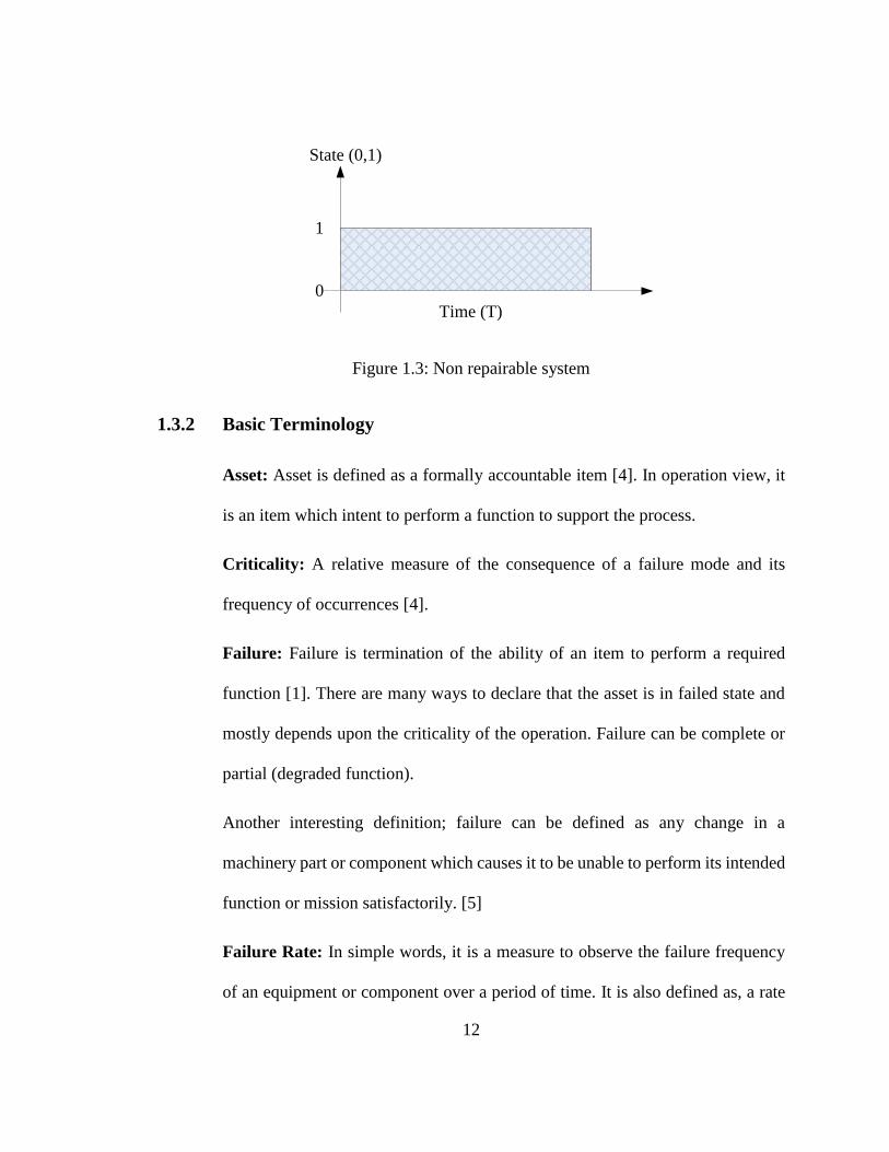
1.3.1.5.2 Non Repairable System
Non repairable systems or components have two states while using in a plant.
The first is functional (working 100%) and other one is non-functional or failed state.
Consider a system that is functional at time 0 and failed at time T, the life of the system or
component will be T. State ‘0’ and ‘1’ represents the failed and function state, as illustrated
in the Figure 1.3. The failure rate of this system is estimated by Equation 1.15.
12
Time (T)
State (0,1)
0
1
Figure 1.3: Non repairable system
1.3.2 Basic Terminology
Asset: Asset is defined as a formally accountable item [4]. In operation view, it
is an item which intent to perform a function to support the process.
Criticality: A relative measure of the consequence of a failure mode and its
frequency of occurrences [4].
Failure: Failure is termination of the ability of an item to perform a required
function [1]. There are many ways to declare that the asset is in failed state and
mostly depends upon the criticality of the operation. Failure can be complete or
partial (degraded function).
Another interesting definition; failure can be defined as any change in a
machinery part or component which causes it to be unable to perform its intended
function or mission satisfactorily. [5]
Failure Rate: In simple words, it is a measure to observe the failure frequency
of an equipment or component over a period of time. It is also defined as, a rate

13
at which failure occurs as a function of time [6]. It is denoted by a symbol λ in
this proposal.
For repairable systems,
𝜆 =1
𝑀𝑇𝐵𝐹 (1.14)
For non-repairable systems;
𝜆 =1
𝑀𝑇𝑇𝑅 (1.15)
Repair Rate: It is a rate that an out of service component will return in service
mode during a given interval. [7]
Unavailability: It is a probability that item or equipment is not in functioning
state. [6]
Mean Time to Failure: It is a basic measure of reliability for non-repairable
items [4]. The total number of system life units, divided by the total number of
events in which the system becomes unavailable to initiate its mission during a
stated period of time. It is denoted by MTTR.
Mean Time between Failures: A measure of system reliability parameter related
to availability and readiness [4]. The total number of system life units, divided by
the total number of events in which the system becomes unavailable to initiate its
mission during a stated period of time. It is applicable to repairable systems. It is
denoted by MTBF.
14
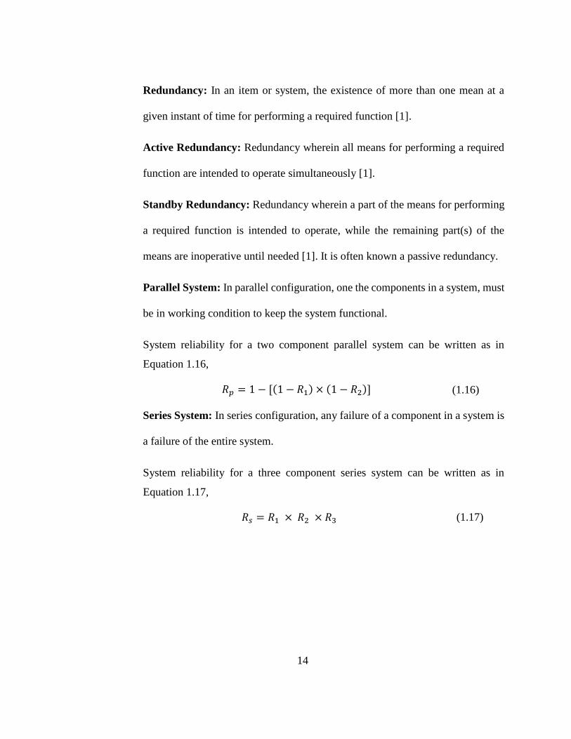
Redundancy: In an item or system, the existence of more than one mean at a
given instant of time for performing a required function [1].
Active Redundancy: Redundancy wherein all means for performing a required
function are intended to operate simultaneously [1].
Standby Redundancy: Redundancy wherein a part of the means for performing
a required function is intended to operate, while the remaining part(s) of the
means are inoperative until needed [1]. It is often known a passive redundancy.
Parallel System: In parallel configuration, one the components in a system, must
be in working condition to keep the system functional.
System reliability for a two component parallel system can be written as in
Equation 1.16,
𝑅𝑝 = 1 − [(1 − 𝑅1) × (1 − 𝑅2)] (1.16)
Series System: In series configuration, any failure of a component in a system is
a failure of the entire system.
System reliability for a three component series system can be written as in
Equation 1.17,
𝑅𝑠 = 𝑅1 × 𝑅2 × 𝑅3 (1.17)

15
1.4 Literature Survey
This Section mainly focuses on the literature survey conducted on availability
estimation and management, early fault detection to improve availability and the role of
maintenance in asset management. Availability estimation and management is not only to
ensure availability of processes but also other important aspects like safety, risk and safe
operations are embedded in the concept. A detailed literature survey is carried out to
highlight the research available in this area and the outcomes are given below.
1.4.1 Physical Asset Management1
The concept of physical asset management (PAM) provides a foundation of
availability management and comprises management of assets such as machines and
equipment in plants. PAM is a systematic approach for managing assets from concept to
disposal; generally termed the asset life cycle. The purpose of a PAM system is to provide
timely information to operations and maintenance personnel to safely increase the total
production output of a plant at a reduced cost per unit of output. These benefits occur as
the manufacturing facility makes optimum operating and maintenance decisions through
the application of a PAM system information solution. Operation and maintenance (O&M)
1Section 1.4.1 is based on the published work in a peer-reviewed proceedings of a gas processing
symposium, Attou, A.K., and Ahmed, Q. (2009), “Asset Management Practices at Qatargas,”
Proceedings of the 1st Annual Gas Processing Symposium, Elsevier B.V. To minimize duplication,
all the references are listed in the reference list. The contribution of the authors is presented in
Section titled, “Co-authorship Statement”.
16
personnel are constantly faced with decision-making based on limited information. PAM
systems make this decision-making job easier by providing knowledge about the current
and future condition of vital production assets. To achieve and meet production
commitments, processing plants are increasingly turning to physical asset management as
an optimization strategy to improve their process efficiency and reduce maintenance, and
so enhancing their return on assets (ROA) [8]. It was noticed during literature survey that
most of the work is performed by industrial experts in engineering magazines; and
international technical journals have limited work available in this area. After realizing the
opportunity, the University of Toronto started a physical asset management program,
which is well received by industry due to the similar reasons for its usefulness and
applicability. As discussed earlier, PAM can reduce maintenance costs, increase the
economic life of capital equipment, reduce company liability, increase the reliability of
systems and components, and reduce the number of repairs to systems and components.
When properly executed, it can have a significant impact on an organization's bottom line
[9].
Companies are reporting as much as a 30 percent reduction in maintenance budgets
and up to a 20 percent reduction in production downtime or unavailability as a result of
implementing a plant asset management strategy. Since as much as 40 percent of
manufacturing revenues are budgeted for maintenance, these savings contribute
significantly to the bottom line of a company. Manufacturers are now moving to implement
such PAM strategies. Industries such as petrochemicals and utilities are aggressively
moving ahead in adopting asset optimization principles [8].
17
The best PAM practices are the premier tools for maximizing availability, customer
satisfaction, budget control, and a firm’s edge over its competitors. In this Section, we
present a PAM framework, experiences, and practices [10]. PAM is a combination of
management, financial, engineering, and maintenance practices applied to physical assets
to achieve low life-cycle cost. A structured approach is required to ensure the best
management of assets. An important motivation for PAM is to achieve best-in-class
reliability and availability, and maintainability of equipment.
It is important to focus on PAM from the early stages of design and development
to reap the real benefits of the approach. Effective asset management typically produces a
20-30% reduction in maintenance cost accompanied by a 15-25% increase in throughput
with no capital investment in equipment [11]. PAM can only be achieved by a team effort.
Before discussing PAM practices, essential terminologies required to comprehend the
PAM practices will be discussed.
It is a common misunderstanding to confuse asset maintenance management
systems (AMMS) with asset performance management systems (APMS). In general, PAM
covers a lot more than AMMS and APMS, but the scope of this Section is limited to
discussion of the AMMS and APMS systems.
1.4.1.1 Asset Maintenance Management System
An AMMS contains information about equipment; its hierarchy in a plant; the
manufacturers; technical and maintenance information including notifications; work

18
history; and spare parts usage. This system is a foundation of PAM and provides
information to APMS to monitor the performance using available data.
1.4.1.2 Asset Performance Management System
An APMS is a tool that provides us the flexibility to use the data in AMMS and
makes it available for analysis. This system monitors performance, maintenance execution,
equipment reliability, process reliability, and availability. The best way to perform this task
is to integrate the system to retrieve data, in an asset-centric approach (ACA) as discussed
in [10] and shown in Figure 2.1.
An asset centric approach is a requirement of AM to streamline the complete process [10].
It is important to have measurement data to manage and control the process. An APMS
provides a platform to monitor performance, whereas AMMS presents a base to capture all
the required data, which includes equipment data, maintenance data, and inspection data.
To implement a successful PAM, it is essential to focus on both AMMS and APMS,
simultaneously. The PAM program mainly focuses on reliability and availability, which
CMMS
(SAP)
Maintenance
Data
Inspection,
Production Data
Monitoring / Scorecards / KPIs
(Meridium)
Asset Maintenance
Management System
Asset Performance
Management System
CMMS
(SAP)
Maintenance
Data
Inspection,
Production Data
Monitoring / Scorecards / KPIs
(Meridium)
Asset Maintenance
Management System
Asset Performance
Management System
Figure 2.1: Asset Centric Approach
19
starts with comprehensive analysis generally referred to as gap analysis. The gap analysis
enables a company to identify its shortcomings. It also provides an estimate to determine
an assignment, which not only fulfills such shortages but also helps optimize the firm’s
AM. Likewise many industrial analyses, including gap, availability, and reliability analyses
are data driven. Therefore, precise data collection is essential to achieve desired outcomes
from these analyses.
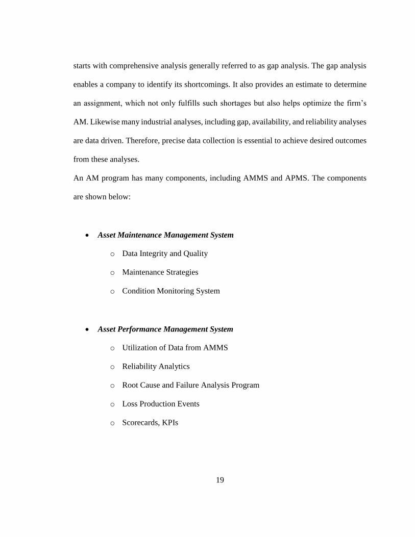
An AM program has many components, including AMMS and APMS. The components
are shown below:
Asset Maintenance Management System
o Data Integrity and Quality
o Maintenance Strategies
o Condition Monitoring System
Asset Performance Management System
o Utilization of Data from AMMS
o Reliability Analytics
o Root Cause and Failure Analysis Program
o Loss Production Events
o Scorecards, KPIs

20
The general strategy to implement PAM in a plant follows the five key steps. A
graphical representation of these key steps is shown in Figure 2.2.
Figure 2.2: General strategy – five key steps
Besides the above mentioned steps, progressive teamwork is essential to a
successful AM program. True success from a PAM program is foreseeable when a firm
adopts a culture of continuous improvement.
This Section briefly discusses the AM practices benefits to natural gas processing
facilities. This effort comprises development of PAM and its implementation, including
benefits and challenges. A significant improvement of availability is experienced with the
implementation of PAM methodology. PAM provides a solid framework to estimate and
manage availability. This Section also deals with the benefits and challenges experienced
during implementation of PAM [10].
Implement (Start)
Monitor
Evaluate
Re-strategize
Sustain (Continue)

21
The benefits that are realized with the implementation of PAM framework:
i. Provides an up-to-date database with maintenance and equipment information
ii. Helps with maintaining lower running costs for the plant
iii. Improved availability and reliability (95-98%)
iv. Proactive rather reactive approach to solving problems
v. Higher profits and customer satisfaction
vi. KPIs and scorecards to monitor performance
Some of the challenges are also identified; outcomes can be improved by addressing them
properly at an early stage of the implementation process.
i. Data capturing, integrity, and quality
ii. Integration among different systems
iii. Cross-function team interaction
iv. Upstream and downstream availability models
1.4.2 Risk and Risk-Based Assessment
To efficiently utilize resources and target poorly performing equipment, risk-
based approaches have been utilized by companies. In these methods, risk is usually
evaluated to identify the action to mitigate them. Chemical processes have great potential
for random equipment breakdowns, system unavailability, production losses, toxic
releases, fire or explosions. Probability of occurrence and the consequences generally are
22
primary drivers of risk analysis for unwanted events. Kaplan and Garrick define risk of an
event as a set of scenarios, each of which has a probability (likelihood) and a consequence
[12]. The likelihood is expressed either as a frequency (i.e., rate of an event occurring per
unit time) or as probability (i.e., the chance of an event occurring in defined conditions),
and the consequence is referred to as the degree of negative effects observed due to
occurrence of an event. To facilitate the risk assessment process, many companies have
developed a risk assessment matrix to quantify risk and its consequences as a baseline to
identify actions to mitigate risk events based on the overall risk.
In general, risk can be calculated using the equation,
𝑅𝑖𝑠𝑘 = 𝑃𝑟𝑜𝑏𝑎𝑏𝑖𝑙𝑖𝑡𝑦 𝑜𝑓 𝑓𝑎𝑖𝑙𝑢𝑟𝑒 × 𝐶𝑜𝑛𝑠𝑒𝑞𝑢𝑒𝑛𝑐𝑒 (1.18)
Risk-based methodologies are commonly used in research and industry to optimize
inspection and maintenance intervals, which maximizes a system’s availability based on
risk. The methodology presented here is comprised of two steps: (i) Availability modeling
and (ii) risk-based inspection and maintenance calculations. A risk-based approach is also
helpful in making decisions regarding prioritization of the equipment for maintenance and
determining appropriate maintenance intervals. The proposed method in this work is
applied to a steam generating system of a thermal power plant. Risk analysis has been part
of a standard operation requirement in the offshore industry for many years. Analyses are
most effective when they are integrated into design work and planning of operations [13].
Risk-based approaches are effective in managing cost, resource planning and return on

23
investment. They are also effectively used in shutdown management to improve plant
reliability and maintain it above a minimum operational reliability [14].
1.4.3 Availability Estimation
Availability estimation is a critical parameter in all aspects of managing
equipment in a plant. It is a main driver for maintenance, operations and others to plan their
respective work. It includes all equipment and systems, and is not limited to production,
engineering, commercial activities and shipping, safety, and machinery. Its importance is
further enhanced by the fact that maintainability with reliability determines the availability
of a plant. A plant must be reliable and easily maintainable to ensure maximum availability,
and should be equipped with the resources needed to bring it back online in the shortest
time in case of any failure. Availability is also important in communication networks and
power networks. In this work, availability models of high-availability communication
networks are discussed. Models were developed to estimate the effectiveness of radio
communication link in achieving its purpose of availability estimation [15].
Availability estimation is vital in planning, maintenance and production of the
processing plant. We will explore some the work performed in the area of availability
estimation in this Section. Most of the equipment in a plant belongs to a repairable system
category and an efficient approach to estimate the availability of the repairable system
within a fixed time period in this work. [16]. Beta distribution has been used to estimate
system availability. The authors applied the proposed model on an IT system. This system
is providing a service to users, where availability is one the critical parameters for

24
monitoring and control. In another effort, availability estimation for an iron ore production
system was performed using simulation. Simulation was used to ensure that the system has
enough redundancies to meet the production requirement [17].
Performance of mining equipment depends on the reliability of the equipment used
and many other parameters like maintenance efficiency, environment, and operator
capability. Reliability analysis is required to identify bottlenecks in the system and to
estimate the reliability of the system for a given designed performance [18]. In this work,
parameters of some probability distribution such as Weibull, Exponential and Lognormal
distribution have been estimated using software. The reliability of critical systems was
identified, which proved to be the main bottleneck in achieving availability of plants.
Modeling of availability for a reliability-based system using Monte Carlo
simulation and Markov chain analysis is presented in this paper [19]. Operational
availability, which is dependent on the mean time to repair and administrative logistic time,
was assessed using breakdown maintenance and scheduled maintenance. The authors have
used the continuous Markov chain analysis for evaluating the probability of each transition
state.
Bayesian estimation of reliability rates was used to estimate the LNG chain
availability [20]. LNG plants usually have very high investment and operating cost.
Improvement of reliability of a LNG chain will lead objectively to a substantial decrease
of energy costs. It is difficult and challenging to model big systems, like LNG chains,
because of their physical dimensions. In this research a systematic approach is used to
discuss the space of the phases. A bottom-up technique was utilized to constitute the global
25
model of reliability of the chain. A Bayesian estimation approach is used to define failure
and repair rates for the equipment. Errors in steady-state availability estimation by 2-state
models of one-unit system, which can be represented by 3-state Makovian models, are
evaluated. It has been concluded that the 2-state models result in large errors for the case
in which degraded systems are not repaired, and so multistate models should be used [21].
Computer simulation is very common in industry to estimate availability and research was
conducted to estimate the availability of a cement plant. Availability is estimated using the
physical configuration of work stations, failure and service time distributing including
buffer storage as inputs [22].
Classical statistical estimation techniques have limited usage in predicting system
availability when a system is highly reliable like a computer. In this work, a Bayesian
solution is suggested to derive both steady-state and instantaneous availabilities [23]. In
refineries and chemical processes, decision making is based on the availability of the
components and entire system. The use of Petri net simulation is common in availability
analysis. In this work, an alternative generic Markov model is used to predict availability
and reduce computational efforts by orders of magnitude [24]. Steady-state series
availability details the importance between the “product rule” and the “correct availability”
[25]. The failure pattern of repairable systems is often modeled by an alternating renewal
process, which implies that a failed component is perfectly repaired. In practice, this is not
true. The paper proposes a generalized availability model using general distribution, which
is different from a new component [26].
26
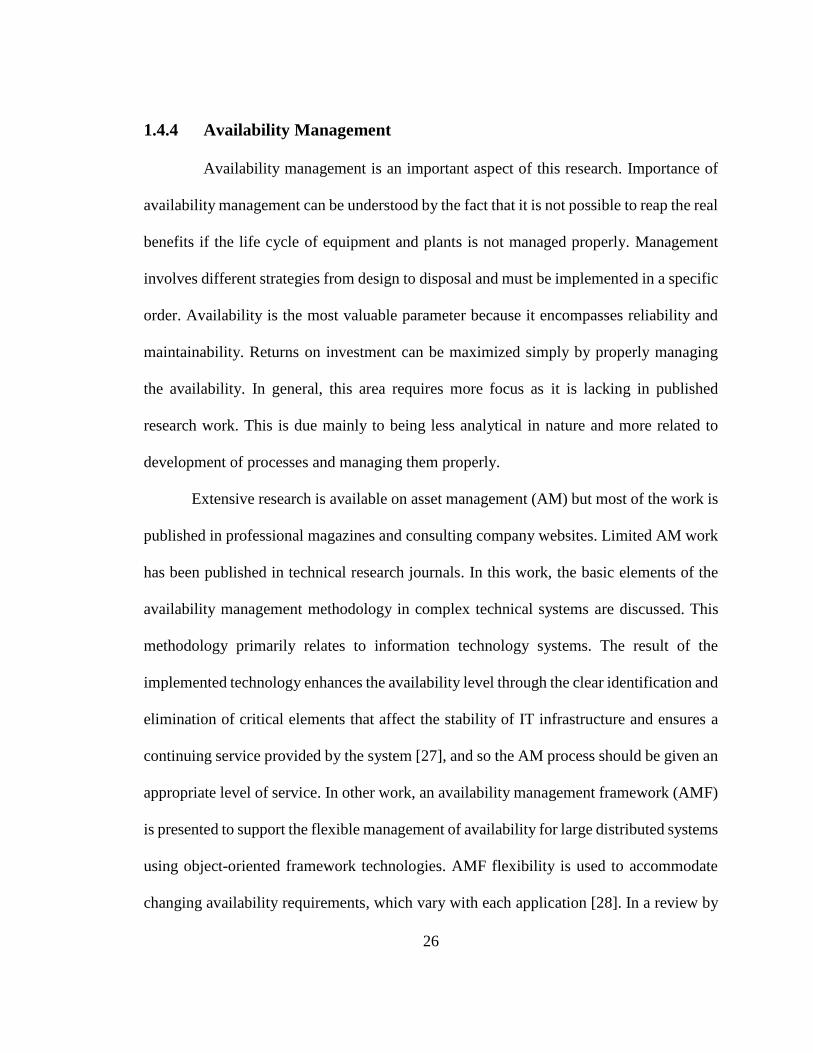
1.4.4 Availability Management
Availability management is an important aspect of this research. Importance of
availability management can be understood by the fact that it is not possible to reap the real
benefits if the life cycle of equipment and plants is not managed properly. Management
involves different strategies from design to disposal and must be implemented in a specific
order. Availability is the most valuable parameter because it encompasses reliability and
maintainability. Returns on investment can be maximized simply by properly managing
the availability. In general, this area requires more focus as it is lacking in published
research work. This is due mainly to being less analytical in nature and more related to
development of processes and managing them properly.
Extensive research is available on asset management (AM) but most of the work is
published in professional magazines and consulting company websites. Limited AM work
has been published in technical research journals. In this work, the basic elements of the
availability management methodology in complex technical systems are discussed. This
methodology primarily relates to information technology systems. The result of the
implemented technology enhances the availability level through the clear identification and
elimination of critical elements that affect the stability of IT infrastructure and ensures a
continuing service provided by the system [27], and so the AM process should be given an
appropriate level of service. In other work, an availability management framework (AMF)
is presented to support the flexible management of availability for large distributed systems
using object-oriented framework technologies. AMF flexibility is used to accommodate
changing availability requirements, which vary with each application [28]. In a review by
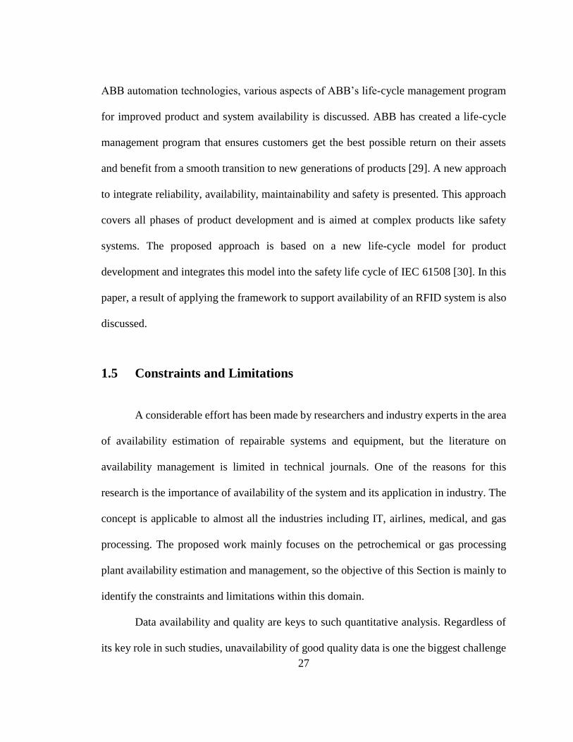
27
ABB automation technologies, various aspects of ABB’s life-cycle management program
for improved product and system availability is discussed. ABB has created a life-cycle
management program that ensures customers get the best possible return on their assets
and benefit from a smooth transition to new generations of products [29]. A new approach
to integrate reliability, availability, maintainability and safety is presented. This approach
covers all phases of product development and is aimed at complex products like safety
systems. The proposed approach is based on a new life-cycle model for product
development and integrates this model into the safety life cycle of IEC 61508 [30]. In this
paper, a result of applying the framework to support availability of an RFID system is also
discussed.
1.5 Constraints and Limitations
A considerable effort has been made by researchers and industry experts in the area
of availability estimation of repairable systems and equipment, but the literature on
availability management is limited in technical journals. One of the reasons for this
research is the importance of availability of the system and its application in industry. The
concept is applicable to almost all the industries including IT, airlines, medical, and gas
processing. The proposed work mainly focuses on the petrochemical or gas processing
plant availability estimation and management, so the objective of this Section is mainly to
identify the constraints and limitations within this domain.
Data availability and quality are keys to such quantitative analysis. Regardless of
its key role in such studies, unavailability of good quality data is one the biggest challenge

28
researchers face when estimating the availability and reliability of systems. In this case,
because of the same reason, a Bayesian approach was used to define the failure rates and
repair rates of different equipment [20]. In the processing industry, the issue of
nonexistence of data is critical [31]. Researchers are using engineering judgments with
available data like OREDA, EXIDA, and other data sources. It is challenging to use
existing data. In case of the OREDA, the data is based on offshore equipment, where the
failure modes are different from the similar equipment installed onshore. Extreme care
must be practiced when using this type of data in validating the proposed models.
Risk is also difficult to calculate because the probability of failure is dependent
upon the quality of the data. As discussed earlier, risk is a product of probability of failure
and the consequence of an event. If the probability calculation is based on poor data, there
is a great chance that all effort can go to waste. Data analysis usually describes statistical
manipulations, which are carried out on raw failure data to provide estimates of component
reliability and availability. All the data analysis gives only limited information if no proper
risk assessment is performed. To determine the safety, reliability, and availability
implications, a proper risk analysis required [32].
To address the above challenges, we have taken extreme care in data collection,
cleansing and analysis. In certain cases, consultation with subject matter experts, along
with personal field experience, was used to ensure the correct data is used in developing
and validating the developed models.

29
1.6 Thesis Structure
This thesis follows the objective sequence as discussed earlier. The Chapter
structure is discussed below:
Chapter 1 provides a brief introduction to physical asset management (PAM);
operation measures like availability, reliability, and maintainability; and other basic
terminology. Section 1.4.1 has detailed discussion on physical asset management.
It attempts to answer why PAM is important and also emphasizes its relationship
with cost, maintenance, and availability management. This Chapter also focuses on
assumptions and limitations; research objectives; a brief literature survey; and the
dissertation structure.
Chapter 2 discusses the overall risk-based availability estimation process using
Markov method. This Chapter includes an introduction to Markov modeling, its
usefulness, and limitations. State models and other modeling work are included in
this Chapter. Analysis results and validation using the gas absorption unit is also
covered.
Chapter 3 describes a novel risk-based failure assessment approach to address the
safety and availability of complex operating systems. A structured process is
proposed and validated using real-world failure assessment cases to prove the
applicability and efficacy of the proposed model.

30
Chapter 4 explored early fault detection and management to support availability
and safety improvement. In this Chapter, decision trees (DTs) are introduced as a
predictive data mining tool to detect early faults and their management to improve
system availability. To conclude the effectiveness of the model, the proposed model
was successfully tested to detect faults using real plant machinery vibration data.
Chapter 5 mainly focuses on multi-constrained, multi-objective maintenance
scheduling optimization. The optimization problem was developed considering a
time-dependent equipment failure rate to optimize maintenance costs at different
availability and reliability levels. These models were applied on a plant scenario to
show the effectiveness of maintenance scheduling optimization on cost,
availability, and reliability.
Finally, Chapter 6 concludes the research with the key findings, novelty and
contributions and suggests possible expansion ideas for this work. This Chapter
also discusses the learnings from this research work and its contribution toward
improvement of industrial issues.
31
CHAPTER 2
RISK-BASED AVAILABILITY ESTIMATION USING A MARKOV
MODEL 2
Abstract
Asset intensive process industries are under immense pressure to achieve a
promised return on investments and production targets. This can be accomplished by
ensuring the highest level of availability, reliability, and utilization of critical equipment in
processing facilities. To achieve designed availability, asset characterization and
maintainability play a vital role. The most appropriate and effective way to characterize
the assets in a processing facility is based on risk and consequence of failure.
2 This Chapter is based on the published work in a peer-reviewed journal. Qadeer Ahmed, Faisal
I. Khan, Syed A. Raza, (2014) "A risk-based availability estimation using Markov method",
International Journal of Quality & Reliability Management, Vol. 31 Iss: 2, pp.106 – 128. To
minimize the duplication, all the references are listed in the reference list. The contribution of the
authors is presented in Section titled, “Co-authorship Statement”.

32
In this Chapter, a risk-based stochastic modeling approach using a Markov Decision
Process (MDP) is investigated to assess processing unit availability, which is referred to as
the Risk Based Availability Markov Model (RBAMM). The RBAMM will not only
provide a realistic and effective way to identify critical assets in a plant but also a method
to estimate availability for efficient planning purposes and resource optimization. A unique
risk matrix and methodology is proposed to determine the critical equipment with direct
impact on the availability, reliability, and safety of the process. A functional block diagram
is then developed using critical equipment to perform efficient modeling. A Markov
process is utilized to establish state diagrams and create steady-state equations to calculate
the availability of the process. The RBAMM is applied to the natural gas (NG) absorption
process to validate the proposed methodology. In the conclusion, other benefits and
limitations of the proposed methodology are discussed.
Acronyms and Abbreviations
Symbol/Abbreviation Description
AS System Availability
AU Unit Availability
Ass Availability – System Static Equipment
AsR Availability – System Rotating Equipment
HP High Pressure
LP Low Pressure
MDP Markov Decision Process
MTBF Mean Time Between Failures
MTTR Mean Time to Repair
33
OREDA Offshore Reliability Data
𝜇 Repair Rate
RA Risk Assessment
RAM Risk Assessment Matrix
RBAMM Risk Base Availability Markov Model
RBD Reliability Block Diagram
SR System Rotating Equipment
SRn Subsystem in Rotating Equipment
SS System Static Equipment
SSn Subsystem in Static Equipment
SHE Safety, Health, and Environment
𝜆 Failure Rate
2.1 Introduction
In the processing industry, high availability and reliability are the means to
effectively utilize and manage processes, equipment, and other resources. This is done to
ultimately improve the return on investment (ROI) for all stakeholders with management
of cost, lowest dangerous emission levels, and highest safety. In recent years, fierce
competition and slim margins have driven economies of scale; companies are trying to
integrate and manage processes while utilizing excess capacities available in other places
to improve upon the availability of the plant. It becomes very critical in the processing
industry to focus on the reliability and availability of the plant to ensure fulfillment of the
global sales commitments with other visionary objectives. In general, availability can be
defined as probability that a system or component is performing its required function at a

34
given point in time or over a stated period of time when operated and maintained in a
prescribed manner [1]. There are many ways to measure and estimate the availability and
reliability of the systems and products. In this work, a processing unit is comprised of many
subsystems incorporating many pieces of equipment. To work on such systems, there are
certain ways to calculate the availability and reliability of the systems. The availability of
the process has embedded reliability and maintainability of the equipment, as in Equation
2.1 and Equation 2.2. To work on availability enhancement and estimation, focus must be
given to both reliability and mean time to failure. Improved availability can be considered
as improved reliability and maintainability. Availability, sometime referred as inherent or
average availability, is measured as:
𝐴 =𝑈𝑝𝑡𝑖𝑚𝑒
𝑈𝑝𝑡𝑖𝑚𝑒 + 𝐷𝑜𝑤𝑛𝑡𝑖𝑚𝑒
(2.1)
𝐴 =𝑀𝑇𝐵𝐹
𝑀𝑇𝐵𝐹 + 𝑀𝑇𝑇𝑅
(2.2)
Processing systems usually consist of many types of equipment, with different
redundancies and architecture to achieve the required level of functionality and availability.
For example, in gas liquefaction systems, the gas is converted into liquid by cooling it
down to a -160°C temperature, and numerous compressors, turbines, motors, vessels, and
valves are utilized to attain this objective [2]. The calculation of availability and reliability
is not an easy task in this type of configuration due to the large equipment base [3]. There
are tools and methods that can be utilized effectively with engineering experience to
35
estimate such parameters. In general, availability can be estimated by considering all the
equipment in a processing unit or plant; given the fact that there are numerous maintainable
pieces of equipment in a processing facility, a detailed monitoring of all equipment is
usually a prohibitive task. In addition, such an investigation of equipment would engage
large amounts of resources both in terms of monitoring systems and personnel. With all
the effort, it may not result in an optimal solution in real-time even with such substantial
investment. But this problem could be solved by using a risk-based assessment approach
that is very effective in identifying the critical systems and handling them appropriately in
a processing plant, as presented in this Chapter.
The goal of this work is to develop a risk-based modeling technique for a
continuous gas processing unit to calculate availability using a Markov methodology and
applying the model to estimate the availability of the gas sweetening Section of a plant, as
in Figure 2.4. The proposed research offers four distinct contributions: first, a risk-based
assessment approach is introduced to identify the most critical components in a typical
plant. Second, using the outcomes of the risk-based assessment; a stochastic modeling
approach based on the Markov Decision Process (MDP) is utilized to develop models that
estimate plant availability. Third, the models developed are calibrated on a gas processing
unit with available plant data and offshore reliability data (OREDA). Lastly, bottleneck
and limiting factors affecting availability will be identified with the benefits of the
proposed methodology.

36
2.1.1 Literature Review
In the literature, extensive work on availability and reliability modeling is available
on repairable equipment but very limited application of full system modeling is observed
in the process industry, i.e., gas processing and other petrochemical facilities. Due to
interest and opportunity, the topic was considered as a means to develop a methodology to
estimate the availability of a complete processing network or unit rather than a single piece
of equipment or a single system. For example, the availability estimation of a gas
compressor as single equipment can be performed easily compared to the complete
liquefaction unit in a gas processing facility.
Availability is widely used in a very generic sense in the existing literature. Many
authors have worked on different availabilities like operational availability, achieved
availability, and inherent availability. Simply, availability is a probability that a system will
be operational when needed to serve a purpose and this usually is termed inherent
availability [4]. Availability has a strong relationship with reliability and maintainability.
Khan et al. [5] proposed a risk-based methodology to maximize a system’s availability by
considering the modeling and risk-based inspection/maintenance calculation. The
discussed methodology is based on two steps: (i) availability modeling and (ii) risk-based
inspection and maintenance calculations. Maintainability has vital importance in
operational availability. Sonawane et al. [6] discussed operational availability where the
mean time to repair and administrative logistic time are important.
Markov analysis is one the many techniques in the literature used to calculate
availability and reliability of multi-state repairable systems. Pil et al. [7] used a time

37
dependent Markov approach to evaluate the reliability of the re-liquefaction system and
developed a maintenance optimization model and applied it to the re-liquefaction system.
Keeter [8] discussed the availability of powerful computers to run long and extensive
models for availability and reliability calculations. These tools have enabled us to
understand the gain achieved from improving equipment reliability, and also other benefits
like asset utilization. Jacob et al. [9] explored the difficulties in determining reliability and
availability for repairable and non-repairable systems. The analysis is difficult when the
failure distribution is not exponential and becomes even more difficult when the systems
are hybrid and complex rather than only series, parallel or a combination of two. In his
work, Jacob presents a binary decision diagram to calculate a system’s reliability and
availability.
Moore [10] pointed out that mechanical availability as a function of maintenance
cost under different maintenance strategies, i.e., the mechanical availability, will be lowest
in reactive strategies and highest in reliability-focused maintenance strategies. Mobley et
al. [11], stressed that availability differs slightly from utilization; the main difference is
that the scheduled run time varies between facilities and is changed by factors such as
schedule maintenance action, logistics and administrative delays. Ouhbi et al. [12] utilized
a semi-Markov system to estimate the reliability and availability of a system and applied it
on turbo-generator’s availability and reliability estimation. Cekyay et al. [13] presented a
work to analyze mean time to fail and availability of mission based system under maximal
repair policy. Csenki [14] explored the concept of work mission availability to approach
the cumulative operational time. Two methods of availability estimation and capacity

38
distribution have been discussed [15]. The first method is based on capacity outage
probability tables, and although estimations performed by this method are exact they have
limited applications. The second method is based on a probability mass function series,
which is computer intensive but the results are better with increasing computation. An
optimal reliability, availability and maintenance management strategy is presented to
optimize the service levels with minimal cost [16]. The focus is on inventory management
and a new model has been introduced to improve the service level, which only covers the
maintainability part of the scope. Availability assessment of offshore oil and gas fields
reveals that the equipment failure and production losses can exceed the allocated budget
[17]. This work explores the probability distribution of downtimes and random equipment
failure in design optimization to improve availability of the production systems. Genetic
algorithms have been used to optimize the availability of the equipment [18]. The
availability optimization was done using different project costs, weight, and availability of
maintenance workforce. The proposed model is a novel and practical contribution, which
presents the risk-based availability estimation using state dependent models.
2.1.2 Brief LNG Process
Liquefied natural gas (LNG) is a liquid form of natural gas. This state of gas
increases its marketability and makes it feasible for transportation around the globe for
utilization in power generation, households and other applications. In liquid form, the
temperature of LNG is usually around -160°C and the volume is around 1/600 times of the
gas at room temperature. It is colorless, odorless and non-corrosive in nature. LNG is
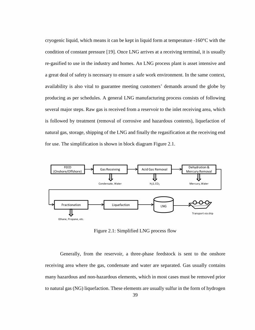
39
cryogenic liquid, which means it can be kept in liquid form at temperature -160°C with the
condition of constant pressure [19]. Once LNG arrives at a receiving terminal, it is usually
re-gasified to use in the industry and homes. An LNG process plant is asset intensive and
a great deal of safety is necessary to ensure a safe work environment. In the same context,
availability is also vital to guarantee meeting customers’ demands around the globe by
producing as per schedules. A general LNG manufacturing process consists of following
several major steps. Raw gas is received from a reservoir to the inlet receiving area, which
is followed by treatment (removal of corrosive and hazardous contents), liquefaction of
natural gas, storage, shipping of the LNG and finally the regasification at the receiving end
for use. The simplification is shown in block diagram Figure 2.1.
Figure 2.1: Simplified LNG process flow
Generally, from the reservoir, a three-phase feedstock is sent to the onshore
receiving area where the gas, condensate and water are separated. Gas usually contains
many hazardous and non-hazardous elements, which in most cases must be removed prior
to natural gas (NG) liquefaction. These elements are usually sulfur in the form of hydrogen
Gas Receiving Acid Gas RemovalDehydration &
Mercury Removal
Fractionation Liquefaction LNG
FEED (Onshore/Offshore)
Condensate, Water H2S, CO2 Mercury, Water
Ethane, Propane, etc.
Transport via ship

40
sulfide, carbon dioxide, water, helium, mercury, other sulfur species and heavy
hydrocarbon. The NG feedstock is treated to remove sulfur and water. Other contaminants
like mercury and mercaptan are removed from the gas prior to the liquefaction process.
Liquefaction of natural gas is a physical process that is achieved by successive cooling
through exchange of heat using refrigerants. LNG is stored in full containment tanks that
are heavily insulated to minimize the heat transfer and boil-off of the liquid. LNG is
shipped through special ships to the destination where it is re-gasified for use in power
generation and returned into country’s gas circuit for home and other domestic use.
2.2 Risk and Risk Assessment
Risk and criticality are two synonyms often used in the oil and gas industry. Risk
can be defined in many ways; simply put, it is the likelihood of an unwanted event times
its unwanted consequence [20]. Risk assessment (RA) is an engineering process of
performing a cross-functional team-based analysis on functions, systems and equipment to
evaluate the risk of a given situation or scenario. In this research, a unique risk assessment
methodology is proposed to effectively select the critical equipment affecting the function
of a system, hence affecting availability. RA is foundation to the proposed research.
Different companies have different exposures to risk depending upon their business,
geographical location, and financial structure and so on. They develop mitigation plans
based on the riskiness/criticality of an unwanted event to avoid them. It is also very
important to understand why the risk assessment is being performed so that attention may
be focused on the right consequences. For example, the oil and gas industry has different

41
financial risks due to its asset intensiveness and price fluctuations compared to other
industries, especially those that do not have physical assets. The industry also has operating
risks and hazards because of high operating pressure and low temperatures. These
operating parameters have severe consequences in case of equipment failure. The risk
assessment approach developed in this research to estimate availability is unique because
the approximation of risk is established using consequences like reliability and
maintainability along with others. The advantage of this approach will provide the benefit
of keeping focus on the categories that directly affect the availability, including others like
safety, health, and environment (SHE), and economics. The main objective of the company
is to identify the risk and develop mitigation plans to address the critical scenarios to as
low as reasonably possible (ALARP) levels. It is not possible to bring the risk to zero, so
importance lies in assessment, mitigation plan and management of risk. Literature and
other standards have defined risk in many ways. The most useful and widely applicable
definition of risk is as follows: “Risk is a measure of potential loss occurring due to natural
or human activities” [20]. Another meaning of risk is a “measure to human injury,
environmental damage or economic loss in terms of both the incident likelihood and the
magnitude of the loss of injury” [21].
The outcome of the risk assessment establishes that either the scenario or equipment
is critical. Riskiness is also known as criticality. The criticality number is a measurement
used to establish whether the assessed scenario or system is critical or not. If the system is
critical, it has to be managed properly to ensure plant target availability. Usually, different
companies have different methods to evaluate risk. One of the most common methods is to

42
evaluate risk using a risk assessment matrix, as shown in Figure 2.2. We used the risk
assessment matrix with four important consequences categories, including: HSE,
Economic (business loss/maintenance cost), Reliability, and Maintainability. It is very
common in the industry to evaluate risk using the first two consequence categories, but the
uniqueness of this risk assessment comes from the consequence categories of reliability
and maintainability, which helps identify the assets that really affect or can affect the
availability of the equipment or processing unit. The details of the risk categories are
explained in Section 2.4.2 of this Chapter. The level to accept risk or level of classification,
i.e., high, medium, or low, depends upon the company management, regulations and other
requirements. The criticality zones shown in the assessment matrix are simply guidelines;
every company has its own risk assessment matrix and defined risk boundary.
Figure 2.2: Risk assessment matrix
Higher consequences mean higher risk and criticality. As an example, if the
consequence is as high as 4 and the probability of the incident is probable as 3, the risk is
high, as shown in Figure 2.2. If the risk is high and the potential threat to the company’s
business or society is high, it must be assessed properly. Risk analysis is mainly used to
estimate the magnitude of a potential loss and can be done by using qualitative or
FREQUENT (4)
PROBABLE (3) HOCCASIONAL (2)
REMOTE (1)
NEGLIGIBLE (1) MINOR (2) MEDIUM (3) HIGH (4) EXTREME (5)
High Medium Low
RISK ASSESSMENT MATRIX
PR
OB
AB
ILIT
Y
CONSEQUENCES
RISK CATEGORIZATION
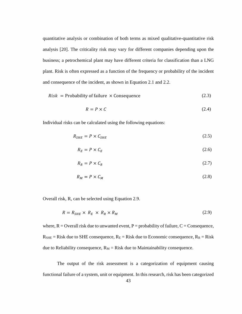
43
quantitative analysis or combination of both terms as mixed qualitative-quantitative risk
analysis [20]. The criticality risk may vary for different companies depending upon the
business; a petrochemical plant may have different criteria for classification than a LNG
plant. Risk is often expressed as a function of the frequency or probability of the incident
and consequence of the incident, as shown in Equation 2.1 and 2.2.
𝑅𝑖𝑠𝑘 = Probability of failure × Consequence (2.3)
𝑅 = 𝑃 × 𝐶 (2.4)
Individual risks can be calculated using the following equations:
𝑅𝑆𝐻𝐸 = 𝑃 × 𝐶𝑆𝐻𝐸 (2.5)
𝑅𝐸 = 𝑃 × 𝐶𝐸 (2.6)
𝑅𝑅 = 𝑃 × 𝐶𝑅 (2.7)
𝑅𝑀 = 𝑃 × 𝐶𝑀 (2.8)
Overall risk, R, can be selected using Equation 2.9.
𝑅 = 𝑅𝑆𝐻𝐸 × 𝑅𝐸 × 𝑅𝑅 × 𝑅𝑀 (2.9)
where, R = Overall risk due to unwanted event, P = probability of failure, C = Consequence,
RSHE = Risk due to SHE consequence, RE = Risk due to Economic consequence, RR = Risk
due to Reliability consequence, RM = Risk due to Maintainability consequence.
The output of the risk assessment is a categorization of equipment causing
functional failure of a system, unit or equipment. In this research, risk has been categorized

44
in three categories, high, medium, and low. Quantitatively, assessment can also be done
using the numbers and selecting the biggest value as the max value as criticality. Once the
ranking has been established, the critical equipment within a system can be chosen and
functional block diagram should be developed to move forward toward a Markov model,
as discussed in the framework in Figure 2.3.
2.3 Risk-based Availability Modeling Framework
The risk based availability concept is based on identifying critical equipment which
causes functional failure in a complex system or unit. Functional failure is an interruption
in production and can be addressed using economic category of the risk assessment matrix.
The proposed framework provides a unique way to identify critical equipment. Asset
intensive unit can be simplified using the risk-based proposed methodology without
violating the functional integrity of the system to estimate availability. The main advantage
of this methodology includes but not limited to identifying the bottlenecks early in the
process and addressing them to optimize resources and cost. Selected systems based on the
risk will pinpoint the equipment that has a direct impact on availability. The system has
many pieces of equipment but not all are critical and should be treated accordingly to
balance the risk and available resources. We will further discuss in detail the Markov based
model to estimate availability.
In order to keep the process consistent and effective, the following steps have been
proposed in this research to develop the model to estimate availability. The graphical
presentation of the complete process can be observed in Figure 2.3.

45
1. Selection of system / operating unit or plant: Develop a boundary diagram of the
system to be studied, which helps team to be focused and prepared.
2. Establish a cross-functional team: Important in order to identify real critical
equipment.
3. Develop or review existing risk assessment matrix to ensure all team members
understand the consequence and probability categories.
4. Perform risk assessment: Ensure risk assessment is done in a cross-functional
environment to identify critical assets.
5. Breakdown of processing unit into small units: After identification of all critical
assets, we developed a functional model to place the equipment in the process
functional flow sequence.
6. Develop functional block diagram to develop state diagram: In this step, a
functional block diagram is developed using the previous step data and represents
the architecture of the systems.
7. Develop a Markov model: State diagrams using functional block diagram are
developed in this step; differential equations are established from the state
diagrams.
8. Collect all required data: The main input of this data is from maintenance history
and other available databases like OREDA [22].
9. Run the model using available failure rate and repair rate data.
10. Estimate availability: Individual subsystems and overall system availability can be
estimated using the independent system data. The series and parallel systems are

46
dealt accordingly to estimate the final availability of the selected system or
operating unit.
2.3.1 Modeling Technique using Markov Model
In general, mathematical modeling of systems is an area of great engineering
interest and process modeling makes it even more challenging. It is not a simple task to
calculate the availability of a unit with a higher number of equipment using individual
equipment failure and repair rates. It is often a model using operating parameters like
production loss, name plate capacity, and sustainable capacity to estimate operational
availability and reliability. The conclusion is usually based on production rates rather than
equipment failure rates. Technically, the outcome is operational availability rather than the
process availability based on the failure date.
The above discussion can be explained further by this example: assuming that you
are assigned to produce 100 tons in 30 days and you are able to produce 100 tons in a given
period with a failure, your availability will be 100% even with a failure. The reason that
the availability is still 100% is that the calculation is based on the production targets rather
than using equipment MTBF and MTTF. The reason you were able to achieve 100%
availability with a failure is that you have utilized your equipment beyond the normal
operating window and were able to achieve the targets. It is indeed a very cumbersome
process to model the complete system and use the real failure rates of equipment for
estimation where the unit consists of thousands of functional locations. The proposed risk
based methodology works great in these situations. Some limitations exist in the proposed

47
Markov methodology, i.e. constant failure and repair rates are independent events and the
probability of being in any state depends upon the immediately previous state.
Figure 2.3: Flow diagram of risk based availability model
As discussed, we will use the failure and repair rates of the equipment and systems
to estimate the availability. This is one of the reasons the risk based approach was adopted
to handle the number of equipment and still obtain reasonable estimates to address the
Select system/process unit
Perform risk assessment
Identify critical systems and
equipments
Develop function block diagram for
critical systems
Breakdown of full system in smaller
functional critical sub-systems
Develop state models (Markov)
Collect data, failure and repair rates
Execute the model
Estimate Availability
Define risk assessment criteria
(RAM)
Establish cross-functional team
Plant failure history
Industrial databases
48
issue. Risk based approach plays a vital role by optimizing the resources and still achieves
comparable results. If a model is developed using 100 pieces of equipment, state space
goes very high and becomes very difficult to handle; as an example, if there are 100 pieces
of equipment and each has 2 states, the total will be 2^100 and that would be around
1.3E+30 states. Quantity can be reduced or the problem can be simplified by breaking
down the system into a series of independent subsystems [3].
In this research, we approach the problem from a user real experience angle and
come up with a risk based approach to estimate process availability. Units have been
broken down into smaller sub-systems to calculate availability, as shown in Figure 2.4.
Markov based state dependent methodology is used to develop state models. A Markov
model is a technique in which a system can be studied with several states, like operational,
failure, and degraded. An approach is presented in this work to estimate the availability of
the unit using different equipment and sub-system individual availabilities within the unit.
State models have been developed using a real plant case, which helped us to model factual
conditions. The proposed method provides a tool to solve the process, which will be
discussed later in the methodology. A Markov model can be mathematically written as
follows [10]:
∑ 𝑅𝑎𝑡𝑒 𝑖𝑛𝑡𝑜 𝑠𝑡𝑎𝑡𝑒 𝑖 𝑓𝑟𝑜𝑚 𝑗 × 𝑃𝑗
.
𝑗
= 𝑅𝑎𝑡𝑒 𝑜𝑢𝑡 𝑜𝑓 𝑠𝑡𝑎𝑡𝑒 𝑖 × 𝑃𝑖
(2.10)
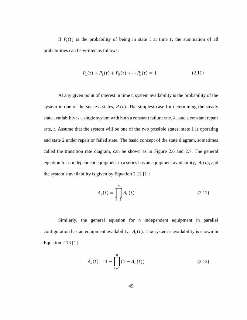
49
If 𝑃𝑖(𝑡) is the probability of being in state 𝑖 at time 𝑡, the summation of all
probabilities can be written as follows:
𝑃1(𝑡) + 𝑃2(𝑡) + 𝑃3(𝑡) + ⋯ 𝑃𝑛(𝑡) = 1 (2.11)
At any given point of interest in time t, system availability is the probability of the
system in one of the success states, 𝑃𝑖(𝑡). The simplest case for determining the steady
state availability is a single system with both a constant failure rate, λ , and a constant repair
rate, r. Assume that the system will be one of the two possible states; state 1 is operating
and state 2 under repair or failed state. The basic concept of the state diagram, sometimes
called the transition rate diagram, can be shown as in Figure 2.6 and 2.7. The general
equation for n independent equipment in a series has an equipment availability, 𝐴𝑖(𝑡), and
the system’s availability is given by Equation 2.12 [1]:
𝐴𝑆(𝑡) = ∏ 𝐴𝑖
𝑛
𝑖=1
(𝑡) (2.12)
Similarly, the general equation for n independent equipment in parallel
configuration has an equipment availability, 𝐴𝑖(𝑡). The system’s availability is shown in
Equation 2.13 [1].
𝐴𝑆(𝑡) = 1 − ∏(1 − 𝐴𝑖
𝑛
𝑖=1
(𝑡)) (2.13)
50
2.4 Application of Proposed Methodology
The proposed methodology has many applications and can be used on any
continuous process, as well as other production processes with some modifications to the
methodology. In this Chapter, the proposed methodology is applied to a gas absorption
process, where high availability is a must in order to safely and economically run the
process. The unavailability of this unit will cause all downstream processes to halt. In order
to apply the methodology in the most effective way, it is essential to review the functional
details of the process to understand the operating nature of the process. It will help to
understand the hazards and their consequences. Secondly, a knowledgeable team with
strong exposure to the process and equipment is required. The foundational step is to
identify the critical components that cause functional failure to the process unit to develop
the model, functional block diagram and other steps as discussed in framework. The
following Section shows the implementation of methodology explored in Figure 2.3.
2.4.1 Brief Description of Absorption Process
A gas sweetening unit is one of the major gas treatment units in a gas processing
plant prior to other processes in the plant like liquefaction, fractionation, and gas
separation. It mainly consists of acid gas removal from the gas stream. This unit primarily
consists of absorption, regeneration and reclaiming Sections. In order to observe the
proposed methodology, we will only focus on the absorption Section of the process. The
simplified block diagram Figure 2.5 explains the functionality.

51
The absorption Section absorbs hydrogen sulphide and carbon dioxide. The
regeneration Section mainly regenerates the solvent and sends stripped out lean acid gas to
the sulfur recovery unit, subsequently; the regenerated solvent is circulated back into the
absorption Section for natural gas sweetening process. Natural gas consists of mainly
gaseous hydrocarbons, partly heavy hydrocarbon and around 1 to 2 percent of acidic gases
like hydrogen sulfide and carbon dioxide and other sulphur compounds. Acidic gases are
highly corrosive and will cause severe damage to cryogenic vessels during liquefaction
process; therefore, it is necessary to remove these gases and contaminants before they reach
the final stages of liquefaction. In the acid gas absorbers, hydrogen sulfide and carbon
dioxide gases are absorbed completely in the solvent and sweet natural gas is routed to the
gas drying Section and liquefaction units. The sour gas from the inlet receiving area enters
in the reception Section where gas is preheated at optimal value to avoid condensation prior
to introduction in the gas sweetening Section. The acid gases enter absorber column where
H2S, CO2 and sulfur compounds are removed by counter current contact of the gases with
a lean solvent in order to meet the required specification of sweet gas. Since the natural gas
sweetening process is very critical in terms of operation and commitment of the LNG
production, the availability of all the equipment remains under focus and operational
integrity is monitored closely. For reliable processing of the gas sweetening unit, all static
and rotating equipment are monitored closely for corrosions due to acidic streams, wall
losses due to erosion caused by high velocities or turbulences. Rotating equipment are
surveyed with their historical records and failure history. To estimate the availability, the
above mentioned framework has been followed in the remaining Section.

52
Sweet Gas - To Next Unit
To Slop pit
Absorber
Column
Gas to Flare
Gas to Incinerator
Ant-foam
Injection Pump
Drain Drum
Solvent
Condensate
Sour Feed Gas
Circulation
PumpsHP Flash
DrumLP Flash
Drum
Lean Solvent
Sour GasSour Gas
HP Recontactor LP Recontactor
Pump A
Pump B
Pump A
Pump B
Washing
Column
From Tank
Rich Solvent
Pump A
Skimming Drains
Rich Solvent
Pumps
Pump A
Pump B
Pump A
Pump B
Skim Oil
Pumps
Rich Solvent
To Flare
HP Solvent
Wet Sweet
Gas
To Exchangers
Figure 2.4: Simplified gas absorption process
2.4.2 Risk Assessment
As discussed earlier, risk assessment (RA) is a systematic approach in performing
risk analysis to identify the failure probability and consequence of the failure due to
exposure to hazards. The goal of RA is to evaluate the magnitude and probability of actual
and potential harm or an actual event [20]. The main hazards in the processing industry are
hydrocarbon, high pressure, high and low temperatures, and poisonous gases. The
consequences can be due to any reason, i.e. equipment breakdown means lower MTBFs,
operating beyond operating windows, higher MTTRs, gas release or human mistakes. This
step is one of the foundations of the complete process. Companies have risk matrix and
risk evaluation methods that can be used to identify critical equipment in a processing unit
and sometimes information is already provided in computerized maintenance management
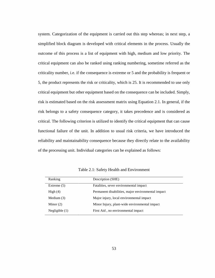
53
system. Categorization of the equipment is carried out this step whereas; in next step, a
simplified block diagram is developed with critical elements in the process. Usually the
outcome of this process is a list of equipment with high, medium and low priority. The
critical equipment can also be ranked using ranking numbering, sometime referred as the
criticality number, i.e. if the consequence is extreme or 5 and the probability is frequent or
5, the product represents the risk or criticality, which is 25. It is recommended to use only
critical equipment but other equipment based on the consequence can be included. Simply,
risk is estimated based on the risk assessment matrix using Equation 2.1. In general, if the
risk belongs to a safety consequence category, it takes precedence and is considered as
critical. The following criterion is utilized to identify the critical equipment that can cause
functional failure of the unit. In addition to usual risk criteria, we have introduced the
reliability and maintainability consequence because they directly relate to the availability
of the processing unit. Individual categories can be explained as follows:
Table 2.1: Safety Health and Environment
Ranking Description (SHE)
Extreme (5) Fatalities, sever environmental impact
High (4) Permanent disabilities, major environmental impact
Medium (3) Major injury, local environmental impact
Minor (2) Minor Injury, plant-wide environmental impact
Negligible (1) First Aid , no environmental impact

54
Table 2.2: Economics, Reliability and Maintainability
Ranking Description (Economics) Description (MTBF) Description (MTTR)
Extreme (5) Downtime > X3 hrs MTBF < Y hrs MTTR > Z3 hrs
High (4) Downtime > X2 < X3 hrs MTBF > Y < Y1 hrs MTTR > Z2 < Z3 hrs
Medium (3) Downtime > X1 < X2 hrs MTBF > Y1 < Y2 hrs MTTR > Z1 < Z2 hrs
Minor (2) Downtime > X < X1 hrs MTBF > Y2 < Y3 hrs MTTR > Z < Z1 hrs
Negligible (1) Downtime < X hrs MTBF > Y3 hrs MTTR < Z hrs
Parameter ranges X, Y and Z in Table 2.2 to rank the consequence are dependent
upon the company business and business guidelines. After the identification of the critical
equipment, the next step is to develop a functional block diagram based on identified
critical equipment, as shown in Figure 2.5. This methodology can be used to include
medium critical equipment in the block diagram depending upon the consequences but it
will increase the size of the model.
2.4.3 Simplified Functional Block Diagram
As discussed earlier, we have selected this system due to the criticality of its
application; presence of poisonous gases, safety impacts on plant and society in case of
unwanted breakdown, including financial consequences. We have presented the unit in
small systems to manage it properly for calculation purposes. This unit consists of
stationary assets and rotary assets as well as piping and valves, as is the case in other oil
and gas processing units. We have developed a block diagram to better understand the
system view of the rotating machinery and static assets in the system. This includes pumps,
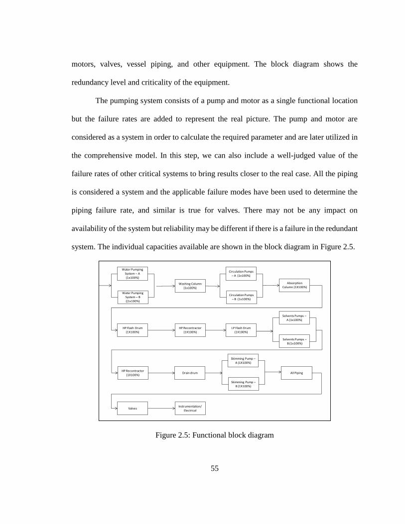
55
motors, valves, vessel piping, and other equipment. The block diagram shows the
redundancy level and criticality of the equipment.
The pumping system consists of a pump and motor as a single functional location
but the failure rates are added to represent the real picture. The pump and motor are
considered as a system in order to calculate the required parameter and are later utilized in
the comprehensive model. In this step, we can also include a well-judged value of the
failure rates of other critical systems to bring results closer to the real case. All the piping
is considered a system and the applicable failure modes have been used to determine the
piping failure rate, and similar is true for valves. There may not be any impact on
availability of the system but reliability may be different if there is a failure in the redundant
system. The individual capacities available are shown in the block diagram in Figure 2.5.
Figure 2.5: Functional block diagram
Water Pumping System – A (1x100%)
Water Pumping System – B((1x100%)
Skimming Pump –A (1X100%)
Skimming Pump –B (1X100%)
Circulation Pumps – A (1x100%)
Circulation Pumps – B (1x100%)
Solvents Pumps –A (1x100%)
Solvents Pumps –B (1x100%)
Washing Column (1x100%)
Absorption Column (1X100%)
HP Flash Drum (1X100%)
HP Recontractor(1X100%)
LP Flash Drum (1X100%)
HP Recontractor(1X100%)
Drain drum All Piping
ValvesInstrumentation/
Electrical

56
2.4.4 Failure Data for Analysis
Failure data is a key to the proposed methodology or even for any statistical
analysis. Equipment’s historical maintenance and repair data availability and quality is an
industry concern, which discouraged us from using the data directly from maintenance
history database. Estimations were developed with the help of engineers and technicians in
order to use the best data. Inconsistency in the available data drove us to get help from
OREDA. OREDA data was not even directly utilized in the analysis but data was sorted
and compiled. The applicable realistic failure modes from the field were identified to
estimate failure rate and repair rates. To effectively model the process and outcome, the
real data and OREDA was utilized together. OREDA database has many failure modes for
any equipment but all are not applicable to every facility. Instead of using all failure modes,
only applicable failure modes were used to estimate the mean failure rate and repair rates.
As an example, OREDA estimates mean time between failures for a pump which is 4 years
based on all failure modes but some of the failure modes are not experienced as per the
failure history. Those failure modes have been taken out to estimate the realistic mean time
between failures. Once taken out the failure modes, mean time between failures improves
to 5 years which is best representative of our case. Active repair rates [22] were used in the
calculation, which refers to the actual time spent on the repair operation rather than the
total downtime or man-hours.
Failure is classified when the equipment is not working or degraded, such as small
leak or passing, when the system is partially available or functional. In vessels, columns
and piping, leaks have taken as a degraded and failed state. Both motor and pump are

57
considered as pumping system in order to avoid confusion because the systems will not
work without one another and will represent the real scenario. All the valves and piping in
the process have been taken as a sub-system and corresponding failure rate and repair rates
have been used to simplify the process. The inclusion of piping and other sub-systems is
also very critical as they experience failures as well to estimate the availability.
Data was used with extreme care, and consideration was given to feasible and
experienced failure modes to estimate the failure rates. In case of rotating machines,
calendar time was used in active systems and operational data was used in standby systems
to be more precise in the calculations. The static equipment data was collected based on
the calendar time, as they were all functional all the time. Availability of the
instrumentation and electrical system is usually very high due to its inherent design so the
system is not selected as part of the process, but the control valves and other emergency
shutdown valves are included in the system. Table 2.3 contains the rotating equipment data,
including both active system failure rates and repair rates as well the standby system rates.
Table 2.4 has all static failure rates and repair rates.
Table 2.3: Rotating Equipment
Code Description Active Failure
Rate
S/B Failure
Rate (/Hr)
Repair Rate
(/Hr)
S/B Repair
Rate (/Hr)
SR1 Pumping System 490.7E-06 13.65 33.0 14.0
SR2 Circulation System 322.4E-06 5.71 28.9 33.7
SR3 Sol. Pumping System 168.9E-06 13.92 7.5 2.5
SR4 A-Foam Inj. System 1.4E-03 - 6.0 -
SR5 Oil Pumping System 1.2E-03 14.9 8.5 7.8
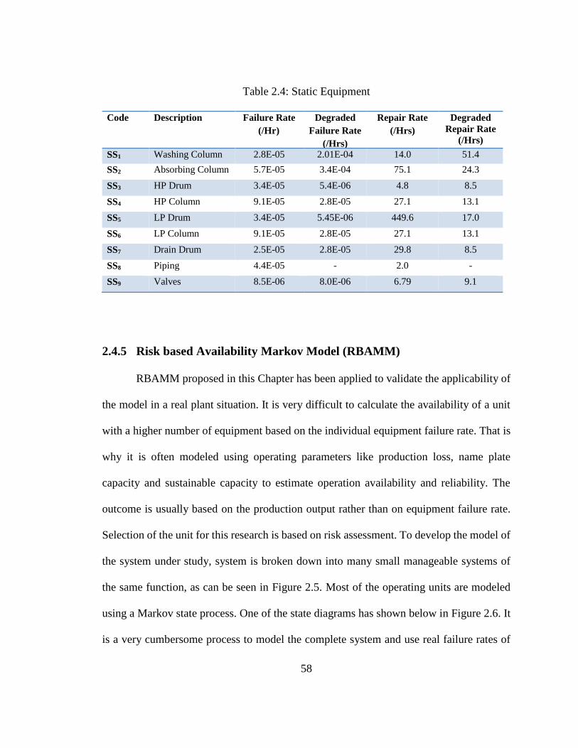
58
Table 2.4: Static Equipment
2.4.5 Risk based Availability Markov Model (RBAMM)
RBAMM proposed in this Chapter has been applied to validate the applicability of
the model in a real plant situation. It is very difficult to calculate the availability of a unit
with a higher number of equipment based on the individual equipment failure rate. That is
why it is often modeled using operating parameters like production loss, name plate
capacity and sustainable capacity to estimate operation availability and reliability. The
outcome is usually based on the production output rather than on equipment failure rate.
Selection of the unit for this research is based on risk assessment. To develop the model of
the system under study, system is broken down into many small manageable systems of
the same function, as can be seen in Figure 2.5. Most of the operating units are modeled
using a Markov state process. One of the state diagrams has shown below in Figure 2.6. It
is a very cumbersome process to model the complete system and use real failure rates of
Code Description Failure Rate
(/Hr)
Degraded
Failure Rate
(/Hrs)
Repair Rate
(/Hrs)
Degraded
Repair Rate
(/Hrs)
SS1 Washing Column 2.8E-05 2.01E-04 14.0 51.4
SS2 Absorbing Column 5.7E-05 3.4E-04 75.1 24.3
SS3 HP Drum 3.4E-05
5.4E-06 4.8 8.5
SS4 HP Column 9.1E-05 2.8E-05 27.1 13.1
SS5 LP Drum 3.4E-05 5.45E-06 449.6 17.0
SS6 LP Column 9.1E-05 2.8E-05 27.1 13.1
SS7 Drain Drum 2.5E-05 2.8E-05 29.8 8.5
SS8 Piping 4.4E-05 - 2.0 -
SS9 Valves 8.5E-06 8.0E-06 6.79 9.1
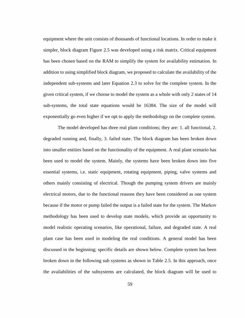
59
equipment where the unit consists of thousands of functional locations. In order to make it
simpler, block diagram Figure 2.5 was developed using a risk matrix. Critical equipment
has been chosen based on the RAM to simplify the system for availability estimation. In
addition to using simplified block diagram, we proposed to calculate the availability of the
independent sub-systems and later Equation 2.3 to solve for the complete system. In the
given critical system, if we choose to model the system as a whole with only 2 states of 14
sub-systems, the total state equations would be 16384. The size of the model will
exponentially go even higher if we opt to apply the methodology on the complete system.
The model developed has three real plant conditions; they are: 1. all functional, 2.
degraded running and, finally, 3. failed state. The block diagram has been broken down
into smaller entities based on the functionality of the equipment. A real plant scenario has
been used to model the system. Mainly, the systems have been broken down into five
essential systems, i.e. static equipment, rotating equipment, piping, valve systems and
others mainly consisting of electrical. Though the pumping system drivers are mainly
electrical motors, due to the functional reasons they have been considered as one system
because if the motor or pump failed the output is a failed state for the system. The Markov
methodology has been used to develop state models, which provide an opportunity to
model realistic operating scenarios, like operational, failure, and degraded state. A real
plant case has been used in modeling the real conditions. A general model has been
discussed in the beginning; specific details are shown below. Complete system has been
broken down in the following sub systems as shown in Table 2.5. In this approach, once
the availabilities of the subsystems are calculated, the block diagram will be used to

60
calculate the total availability of the system. The advantage of separately calculating the
static, rotating and other equipment will provide the flexibility to identify if any one of the
systems is a bottleneck and requires more focused work to improve availability and
reliability. There are many different operating scenarios that can be easily modeled using
a Markov process. In this system, two different systems available were commonly used
during the Markov modeling process. Pumping systems with redundancies were modeled
using the state diagram shown in Figure 2.6, and a non-redundant system i.e. Absorber
Column, is modeled with three operating states as in Figure 2.7. In this model, state 1
represents the equipment is functional as designed and state 2 reflects the equipment is
working but not meeting the functional requirements. For example, valve is passing and
process is still functional with degraded performance. State 3 represents the complete
failure where the repair is inevitable. At state 3, once the equipment is repaired the system
goes back to state 1, and from this state system cannot go back to degraded state. Once the
system is fixed, it will only go to its initial state 1.
Figure 2.6: State diagram of two pieces of equipment in parallel with failure in standby
1
3
4
2
A/B Functional
Failed
λ1
r1 r2
λ2
λ2
r2λ1
r1
A F
aile
d
B Failed
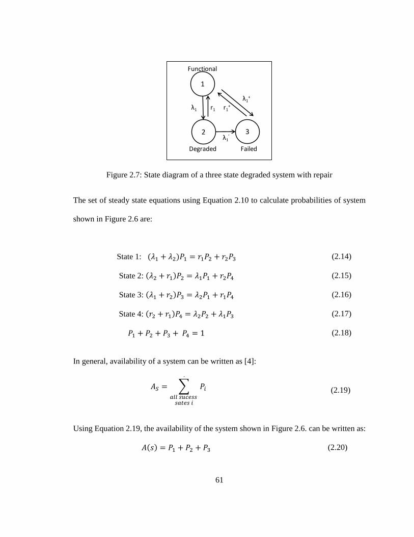
61
Figure 2.7: State diagram of a three state degraded system with repair
The set of steady state equations using Equation 2.10 to calculate probabilities of system
shown in Figure 2.6 are:
State 1: (𝜆1 + 𝜆2)𝑃1 = 𝑟1𝑃2 + 𝑟2𝑃3 (2.14)
State 2: (𝜆2 + 𝑟1)𝑃2 = 𝜆1𝑃1 + 𝑟2𝑃4 (2.15)
State 3: (𝜆1 + 𝑟2)𝑃3 = 𝜆2𝑃1 + 𝑟1𝑃4 (2.16)
State 4: (𝑟2 + 𝑟1)𝑃4 = 𝜆2𝑃2 + 𝜆1𝑃3 (2.17)
𝑃1 + 𝑃2 + 𝑃3 + 𝑃4 = 1 (2.18)
In general, availability of a system can be written as [4]:
𝐴𝑆 = ∑ 𝑃𝑖
.
𝑎𝑙𝑙 𝑠𝑢𝑐𝑒𝑠𝑠 𝑠𝑎𝑡𝑒𝑠 𝑖
(2.19)
Using Equation 2.19, the availability of the system shown in Figure 2.6. can be written as:
𝐴(𝑠) = 𝑃1 + 𝑃2 + 𝑃3 (2.20)
2
1
3
Degraded Failed
Functional
λ1
λ1’
λ1+
r1 r1+
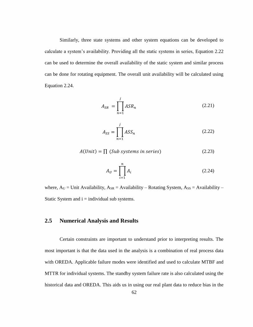
62
Similarly, three state systems and other system equations can be developed to
calculate a system’s availability. Providing all the static systems in series, Equation 2.22
can be used to determine the overall availability of the static system and similar process
can be done for rotating equipment. The overall unit availability will be calculated using
Equation 2.24.
𝐴𝑆𝑅 = ∏ 𝐴𝑆𝑅𝑛
𝑗
𝑛=1
(2.21)
𝐴𝑆𝑆 = ∏ 𝐴𝑆𝑆𝑛
𝑗
𝑛=1
(2.22)
𝐴(𝑈𝑛𝑖𝑡) = ∏ (𝑆𝑢𝑏 𝑠𝑦𝑠𝑡𝑒𝑚𝑠 𝑖𝑛 𝑠𝑒𝑟𝑖𝑒𝑠) (2.23)
𝐴𝑈 = ∏ 𝐴𝑖
𝑛
𝑖=1
(2.24)
where, AU = Unit Availability, ASR = Availability – Rotating System, ASS = Availability –
Static System and i = individual sub systems.
2.5 Numerical Analysis and Results
Certain constraints are important to understand prior to interpreting results. The
most important is that the data used in the analysis is a combination of real process data
with OREDA. Applicable failure modes were identified and used to calculate MTBF and
MTTR for individual systems. The standby system failure rate is also calculated using the
historical data and OREDA. This aids us in using our real plant data to reduce bias in the

63
results. Proposed methodology helps to calculate the availability of the individual sub
system and can be used to identify bottleneck in the system. Table 2.5 shows the
availability of the individual subsystem whereas Table 2.6 shows the availabilities of static
and rotating as well the unit availability. In the existing approach to estimate availability
at facility, it is very difficult to calculate the individual availability of the subsystems, but
the proposed methodology has the flexibility to estimate all availabilities.
Table 2.5: Individual Availabilities of Subsystems
Code Description Availability
SR1 Water Pumping System 0.945
SR2 Water Circulation System 0.998
SR3 Solvent Pumping System 0.909
SR4 Anti-Foam Inj. System 0.995
SR5 Skim Oil Pumping System 0.768
SS1 Water Washing Column 0.957
SS2 Acid Gas Absorbing
Column
0.968
SS3 High Pressure Drum 0.999
SS4 High Pressure Column 0.947
SS5 Low Pressure Drum 0.999
SS6 Low Pressure Column 0.947
SS7 Drain Drum 0.926
SS8 All Piping 0.999
SS9 Valves 0.999
Steady states equations were developed using Equation 2.1 and solved by using
Excel to calculate probabilities of certain states to estimate the availability of subsystems.
Once the availabilities have been judged, Equation 2.11 is used to determine the availability
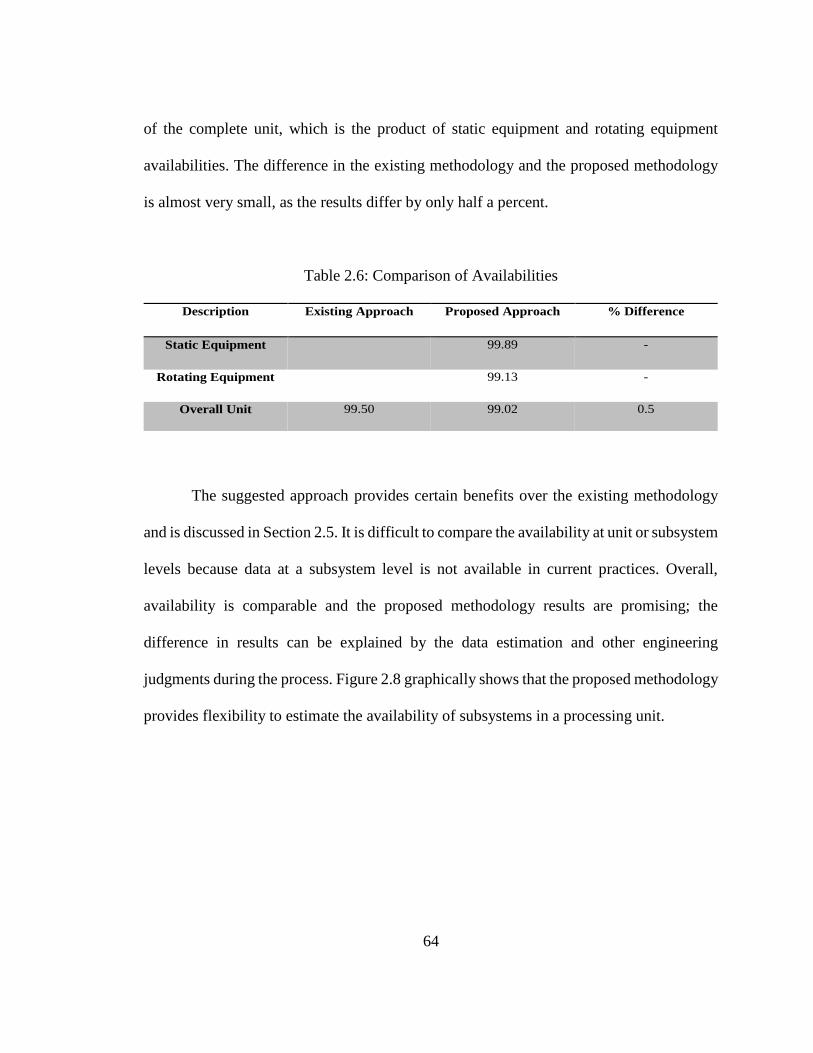
64
of the complete unit, which is the product of static equipment and rotating equipment
availabilities. The difference in the existing methodology and the proposed methodology
is almost very small, as the results differ by only half a percent.
Table 2.6: Comparison of Availabilities
The suggested approach provides certain benefits over the existing methodology
and is discussed in Section 2.5. It is difficult to compare the availability at unit or subsystem
levels because data at a subsystem level is not available in current practices. Overall,
availability is comparable and the proposed methodology results are promising; the
difference in results can be explained by the data estimation and other engineering
judgments during the process. Figure 2.8 graphically shows that the proposed methodology
provides flexibility to estimate the availability of subsystems in a processing unit.
Description Existing Approach Proposed Approach % Difference
Static Equipment 99.89 -
Rotating Equipment 99.13 -
Overall Unit 99.50 99.02 0.5

65
Figure 2.8: Graphical comparison of availabilities
Prior to the proposed methodology, unit availability is a value, which is 99.5%, and
represented by a straight line. It was difficult to estimate subsystem availabilities quickly
to identify the bottleneck and area of concern. With the proposed scheme, subsystems
availabilities are estimated from the start, which makes it easier to identify areas of concern
and efficient utilization of resources.
2.5.1 Advantages and Limitations of Proposed Methodology
The proposed methodology has shown very promising results and comparable to
existing availability of the processing unit with other important benefits. The advantages
mentioned below provide better control and understanding of the processing unit. Some
0.7
0.75
0.8
0.85
0.9
0.95
1
1.05
SR1 SR2 SR3 SR4 SR5 SS1 SS2 SS3 SS4 SS5 SS6 SS7 SS8 SS9
Av
aila
bili
ty
Systems in Unit
Calculated Vs Unit Availability
Calculated Availability
Unit Availability

66
supremacy of the risk-based proposed methodology has been proven and is discussed
below.
a. Efficient planning tool; allocation of resources as the individual asset system
availabilities are available to identify poor performers as shown in Figure 2.8. Poor
performing systems can easily be identified and detailed analysis can be performed.
b. Identification of real plant critical equipment that affect the availability of the plant.
c. Prioritization of the maintenance work based on criticality classification.
d. Risk assessments performed can be used in reliability centered maintenance
activities.
e. Long term planning, once plant model is developed; quick identification of bad
actors.
f. Initiative to enhance the maintenance history data program.
g. Better spare parts and maintenance planning to reduce MTTR.
h. Effective tool to optimize turn around and inspection shutdown.
The proposed framework is flexible and easy to use when using the step by step
process discussed in Section 2.3. Proper attention must be given to step by step execution
while performing studies using this approach. The risk matrix used in risk-based
assessment must reflect the company risk criteria rather than individual departmental
criteria. It is an experience that different departments have their own risk matrices to
prioritize their work. Use of the matrix ensures that the experienced personnel are involved
in performing risk assessment with good understanding of the system and its failure
67
consequences. Failure history data must be used with care and questionable data must be
scrutinized or normalized properly. The state models must consider all the experienced
failed states to obtain more realistic results.
2.6 Conclusion
Many methods have been discussed in the literature review to estimate the
availability of independent systems, but efforts toward the estimation of processing
facilities, like gas plants or refineries, were found to be limited. The proposed methodology
establishes an efficient and effective way to manage assets, as well as estimate and improve
availability. The suggested approach to estimate the availability using RBAMM of a
processing unit is unique and has shown promising results compared to existing
methodology. The exclusivity of this proposal is the risk-based approach, which tends to
alleviate the data scarcity situation by selecting the critical equipment in a unit and utilizing
the failure databases smartly.
The method discussed addresses a real field issue and provides a solution to the
issue with a high level of confidence. Data was reviewed and adjusted based on engineering
judgment in conjunction with OREDA to make it suitable for use. This methodology
provides an opportunity to identify subsystem availability, which helps us identify the true
bottleneck in a processing unit. The proposed research engages the issue of calculating the
availability of a continuous operating plant. The model is validated on the real
configuration of the plant and the real operating scenarios so that the results will be

68
realistic. This research also highlights the need and importance of good quality
maintenance history and effective utilization of the existing data to perform similar studies
with more confidence.
A risk-based methodology can be extended to develop a computer application using
the proposed approach for operating plant use. It is an optimal risk based solution for users
to efficiently utilize resources and achieve better results with less operating cost. The
effective utilization of the suggested method will help reduce cost and improve plant
reliability and availability.
69
CHAPTER 3
IMPROVING AVAILABILITY USING A RISK-BASED FAILURE
ASSESSMENT APPROACH 3
Abstract
A structured risk-based failure assessment (RBFA) approach is presented, which
provides a complete solution to avoid repeated and potential failures to improve overall
plant safety and availability. Technological advancements and high product demand have
encouraged designers to design mega-capacity systems to enhance system utilization and
improve revenues. These benefits make the systems more complex and so prone to failure.
3 This Chapter is based on the published work in a peer-reviewed journal. Qadeer Ahmed, Faisal
Khan, Salim Ahmed (2014), “Improving safety and availability of complex systems using a risk-
based failure assessment approach,” Journal of Loss Prevention in the Process Industries, Volume
32, November 2014, pages 218-229. To minimize the duplication, all the references are listed in
the reference list. The contribution of the authors is presented in Section titled, “Co-authorship
Statement”.
70
In general, despite the elaborately planned maintenance and monitoring activities,
equipment still fails. In reality, it is an overwhelming task to address all the failures due to
limited resources and time constraints. This leads to substandard and poor quality failure
assessments, which cause repeated failures. To address this common industry concern, a
four phase RBFA framework is proposed, which is not limited to the identification of root
cause(s) but also includes all the other actions essential for a successful assessment. The
four phases include the plan phase, the assessment phase, the analysis phase, and the
implementation-tracking phase. These phases cover identification of failure and failure
analysis; root cause(s) along with corrective actions are mooted, prioritized, and monitored
for implementation. In this Chapter, the applicability and advantages of the proposed
approach are examined through two real case studies pertaining to bearing failure and drive
coupling failure. Significant improvements have been experienced in the mean time
between failure (MTBF) and system availability for both the cases.
3.1 Introduction
In a processing facility, equipment and systems are anticipated to perform their
function safely and reliably to meet production requirements. Despite the best maintenance
and operating strategies, systems and equipment fail. These failures must be analyzed
properly to identify the root cause(s) and implement corrective actions to avoid repetition.
Repeated failures are very common where the failure assessment is done poorly and
corrective actions are implemented without proper validation of the root cause(s). In a

71
study [1], the failure history shows that the fuel oil pump experienced 14 failures during
an operating life of 10 years. In another study of repeat failures, the authors mentioned that
18 events of compressor failures occurred during the last 12 years. These examples
highlight the fact that failure investigations are either not handled properly or corrective
actions are not implemented properly. A thorough and structured investigation process is
therefore needed to avoid the general problem of repeated failures [2].
Failure is defined as an “inability to perform the intended function,” whereas a fault
is “an abnormal condition or defect at the component, equipment or subsystem level, which
may lead to a failure” [3-4]. Risk-based failure analysis in this work is defined as, “a
structured process that discovers root cause(s) — physical, human, or latent of an incident
(failure or fault) and addresses these causes with corrective actions to improve the
availability and safety of the workplace.” Failure and availability are two sides of a coin;
reduction in equipment failures greatly improves the availability of the system and vice
versa. Failure can be eliminated or reduced by effective maintenance, adequate operation,
proper design, and other parameters. In case of a failure, proper failure investigation is
important to identify and eliminate the root cause(s). Availability improvement is neither
one size fits all nor a piece of technology or software solution; it is a strategic objective to
be met. Therefore, all the factors affecting availability are essentially considered with their
importance. An appropriate combination of assessment approach, tools, and technologies
is vital to reduce failures but the list also contains skills and good planning to achieve this
goal. Availability suggests the readiness of the system when required. Many factors affect
the readiness of the system, including planned downtime for preventive maintenance,

72
unplanned breakdowns, and availability of spares. Availability can be significantly
improved by reducing the equipment downtime by either addressing reliability or
maintainability [5]. A major factor of poor availability is repeat failure or recurrence of a
failure, which can be reduced by a structured and smarter root cause analysis approach,
with the assurance that the corrective actions have been implemented. Analyzing failures
correctly improves the failure rate, which means minimization of downtime and repair
time, ensuring better mean time between failures (MTBF) and mean time to repair (MTTR)
as represented in Equations 3.1 and 3.2.
𝐴𝑣𝑎𝑖𝑙𝑎𝑏𝑖𝑙𝑖𝑡𝑦 (𝐴) = 𝑈𝑝𝑡𝑖𝑚𝑒
𝑈𝑝𝑡𝑖𝑚𝑒 + 𝐷𝑜𝑤𝑛𝑡𝑖𝑚𝑒 (3.1)
Availability can also be written as,
𝐴𝑣𝑎𝑖𝑙𝑎𝑏𝑖𝑙𝑖𝑡𝑦 (𝐴) = 𝑀𝑇𝐵𝐹
𝑀𝑇𝐵𝐹 + 𝑀𝑇𝑇𝑅 (3.2)
where, MTBF = Mean Time Between Failures and MTTR = Mean Time to Repairs
Equation 3.2 can also be expresses as,
𝐴𝑣𝑎𝑖𝑙𝑎𝑏𝑖𝑙𝑖𝑡𝑦 (𝐴) =𝜇
(𝜆 + 𝜇) (3.3)
where, λ = Failure Rate and µ=Repair Rate
73
As an illustration, an improvement in MTBF by 90 days and repair time by 5 days
in a year, results in an overall availability improvement of 2.5%. Highly structured failure
analysis approaches are required to achieve such objectives in asset intensive industries
like gas processing, nuclear, and aerospace.
Failure analysis is a multifaceted and challenging task but with a structured
methodology, knowledgeable and skilled team, the real root cause(s) can be efficiently
identified. The identification of the root cause(s) does not lead to the conclusion of the
objective because the real solution is to develop corrective actions and to implement them
to avoid repeat failures. A structured approach is a way to analyze failures because
unstructured processes only support opinions and are unable to produce lasting results. As
a result, supporting a structured approach in problem solving is highly desirable [6]. Failure
consequences drive the classification of the failure investigation. Classification is required
so that the investigation can be performed based on the criticality of the failure. Failure
investigation can be classified by the importance and criticality of a failure, which derives
the need of a detailed analysis [7]. Based on the risk consequences, failure analysis is
categorized as high, medium, or low. Brief investigations are performed on non-critical
failures whereas a detailed analysis is required on critical failures along with effective
management of the corrective actions. Investigations limited to only identifying the reason
of a material failure and restricted to a component analysis are usually classified as
component failure analysis and do not address the system issues. For example, a bearing
analysis is performed and the result indicates a lack of lubrication but the reasons of the
lack of lubrication are not discussed. Root cause(s) investigation covers other causes, i.e.,

74
human causes but does not explore the latent causes. Root cause and failure analysis cover
all three areas of cause identification as discussed above but still the other parts of the
complete process are not included. In this research, a complete failure analysis process,
risk-based failure assessment, is proposed that starts from a failure or fault event, to
identification of root cause(s), to implementation of recommendations and extends up to
the effectiveness of corrective actions. In this Chapter, a four-phase RBFA framework is
proposed, which is not limited to the identification of root cause(s) only but also includes
all the other actions essential for a successful assessment. The applicability and advantages
of the proposed RBFA approach are examined through two case studies pertaining to
bearing failure and drive coupling failure.
The remainder of the Chapter is organized as follows: Section 3.2 explores the
research work done in this area. Section 3.3 discusses the risk-based failure assessment
framework. Section 3.4 presents two case studies to observe the application of proposed
approach and the results. Section 3.5 discusses the critical success factor of the proposed
methodology. At the end, in Section 3.6, a conclusion and contributions are discussed.
3.2 Background Study
Failures and faults are the most undesirable events that adversely affect the
availability of an operating facility. To avoid such events, engineers do their best to
effectively operate and maintain the system. Many tools such as condition monitoring and
process monitoring are available to proactively predict and analyze such unwanted events

75
but failures still exist. Along with other efforts, proper failure analysis is the key to address
these unwanted events by identifying the real root cause(s) along with developing and
implementing corrective actions.
In industry, many tools are available to carry out root cause analysis of a failure.
Some of the common tools employed are 5 Whys, Fault Tree Analysis, Ishikawa Diagrams
(commonly known as Fishbone Diagrams), and Failure Mode and Effects Analysis
(FMEA). Use of these tools is questionable as witnessed by many recurrences and repeated
failures. In one study, the performance of three popular root-cause analysis tools namely,
Cause-and-Effect Diagram, the Interrelationship Diagram, and the Current Reality Tree
were analyzed [8]. It was found that these tools have the capacity to find root causes with
varying degrees of accuracy and quality due to their individual unique characteristics and
application constraints. In the literature, different methodologies have been used to
estimate the availability ranging from fault detection, reliability block diagrams, FMEA,
fault tree analysis, and so forth [2, 9, 10, and 11]. A great opportunity exists in addressing
system availability using a risk-based systematic approach, which is proposed in this work.
Production pressure and operating constraints necessitate that investigations must be
completed quickly. Quick complex failure analysis contributes to repeated failures and
wrong root cause(s) due to limited focus on identification of the real root cause(s),
accepting or rejecting all failure possibilities, and bypassing a structured failure
investigation. The other common problem is the lack of focus on the implementation of
corrective actions, which is one of the major contributors to repeated failures. In this work,
there is more focus on the "operate and maintain phase," which is truly the longest phase

76
in the life-cycle of equipment as shown in Figure 3.1. The proposed model can be used
effectively to assess potential failures or conditions in design and construction.
Figure 3.1: Availability – operate and maintain
Fault Tree Analysis (FTA) is a top-down failure investigation approach to perform
studies to improve the availability, reliability, and safety of the systems. The approach
discussed in [12] does not provide a holistic solution to address repeated failures and
availability. In another work, plant safety and availability improvement is suggested using
reliability engineering tools [13]. In this technological era, signal processing has been
proven to be very effective in performing fault diagnostics and prognostics to improve
availability and maintainability of complex operating systems. The Kalman filter based
ensemble approach is used to predict the remaining useful life of a turbine blade creep
degradation process [14]. Stochastic models are great in predicting the useful life of
equipment, but they lack an approach for addressing real plant failure causes. Prognostic
and health management is a research area that may provide a solution and guidance to
industry to maintain the availability of the systems, safety, and economics of the operating
facilities. A technical framework of equipment health management based on six key
elements during the design stage for complex mechanical systems is proposed [15]. A
Availability Analysis
Design Construction
Operate and Maintain
77
comparison between the traditional and proposed health management framework is
performed along with validation using case studies, which works well proactively to avoid
failure rather than assess failures. In an another effort, a novel and highly sophisticated
layered dynamic hybrid fault modeling and extended evolutionary game theory is proposed
for reliability, survivability, and fault tolerance analysis [16]. Due to the complexity and
sophistication, the authors have recommended developing software to implement such a
sophisticated model for ensuring the integrity of the modeling technique. Complex and
highly advanced tools sometime hinder efforts and make it difficult to analyze failure
effectively. To evaluate the consequences of a certain fault or failure, risk is an important
aspect to evaluate in complex systems. To study the relationship between risk, availability
and its consequences in certain scenarios, a risk-based availability analysis model is
presented [17]. The proposed model helps in maximizing reliability and improving the
maintainability of systems, which enhances availability as shown in Equation 3.2.
Avoidance of repeated failures improves reliability and availability, which can be easily
achieved by proper failure investigation and implementation of the recommendations of
this study. As proposed in [18], a risk-based availability model is used to optimize
maintenance strategies. In this work, imperfect maintenance has been discussed in context
with equipment availability. Virtual age models of imperfect maintenance are used to
estimate the availability of the equipment. An availability model of repairable equipment
based on virtual age is defined and, by using a simulation availability function, availability
is estimated. Imperfect maintenance is also a source of failure and requires proper attention
to improve maintenance. In another study, a model for fault detection and availability in

78
complex services is investigated [19]. A realistic reliability model to study the asset
allocation problem to obtain the desired level of availability is presented. The model is
validated using a real case of a multimedia communication service.
As discussed above, many different techniques and methodologies are presented to
estimate availability but limited work seems to have been done to address availability using
proper failure analysis. In this Chapter, a risk-based failure analysis approach is proposed,
which addresses the issue of an equipment failure, repeat and potential failures to enhance
availability. This approach is based on a structured risk-based process, which helps in
streamlining the process of identifying the real root cause(s), and to develop and prioritize
corrective actions for implementation.
3.3 Risk-Based Failure Assessment (RBFA) Framework
Reducing risk and improving availability are the prime objectives of any
processing facility. Risk can greatly be reduced by avoiding repeated and potential failures.
A structured and robust risk-based failure assessment process is a result-oriented tool to
address this issue. Failure assessment is one of the basic availability enhancement tools
and can be performed in formal and informal setups [20]. To effectively use the assessment
process, the classification of failure is required. It is extremely important to conduct the
assessment either formally or informally to ensure the optimal and efficient use of the
resources. The classification of a failure drives the criticality of the failure and suggests the
level of failure investigation required. In certain cases, a simple process is an effective way
79
to perform failure assessment and on the other hand, in critical cases, a thorough
investigation with irrefutable evidences and a knowledgeable team has to be conducted to
uncover the real root cause(s). An RBFA approach presented covers the complete process
of failure assessment and enables us to use the optimal way of performing failure
investigations. The proposed assessment process does not only cover the failure analysis
and identifies the root cause (s) but it also provides a complete business process from
identification, resolution to the avoidance of repeat failures. In complex plants and
machines, failures have significant consequences and the equipment can fail in many ways,
which requires the active involvement of knowledgeable personnel in the investigation
process. The RBFA approach suggests performing failure assessment based on its
criticality and the consequences of a failure. The risk-based philosophy helps in addressing
the critical failures as formal and the non-critical ones as informal, which ultimately help
organizations to allocate the right resources to high risk events. Proper investigation of all
incidents and identification of the real root cause (s) is essential to avoid them in future;
hence helping improve availability. The complete RBFA process has been divided into
four phases and nine steps within the phases to elaborate the proposed methodology. The
four phases and their steps are discussed below and are shown in Figure 3.2. The complete
methodology of RBFA and recommendation management is discussed in Figure 3.3.

80
3.1.1 Plan Phase
The planning phase is the most important phase in the proposed RBFA approach.
Proper planning helps in understanding and defining the scope of the investigation. This
phase provides the opportunity to have a first-hand feel and sets the stage for what to do
and how to do it. This phase mainly covers the identification of an incident (failure) or
potential incident (fault), and the collection of preliminary information. This phase
provides the foundation upon which the remaining phases can be built. It has a significant
impact on the complete approach. The three steps in this phase are as follows:
3.1.1.1 Identify and Record Failure/Fault
The first step in this phase is to identify and record an unwanted event i.e., a
failure or a fault. The incident must be recorded in the maintenance management system
or any other designated system with the basic failure information such as failure
Figure 3.2: Four phases – risk-based failure assessment

81
description, time, equipment number, and consequences of the failure. In order to develop
a formal system, a separate platform is introduced and interfaced with asset performance
management and asset maintenance management system [21]. The system facilitates the
investigation process for proper execution and control.
3.1.1.2 Preserve Site and Data
The second step in this phase is to preserve the failure site and basic data. This
step is critical in the investigation because it is in this step that the failed equipment is
thoroughly observed, data is collected, pictures are taken for future reference and shared
with the team during formal investigation. Failure assessment quality is dependent on the
quality of the information. Therefore, the focus must be given to the right information from
trustworthy sources.
3.1.1.3 Collect Preliminary Information
Good quality, realistic information is the core of an effective investigation
process. During the planning phase, the preliminary and basic data must be collected prior
to moving forward to the assessment phase. Preliminary data includes, but not limited to,
equipment history, process flow diagrams, operating conditions, and process
instrumentation diagrams. It may include interviews for the operation and maintenance to
collect all the basic information.
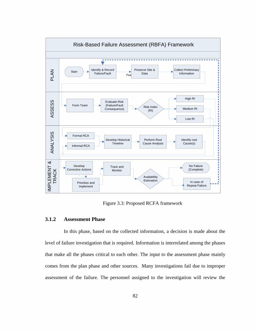
82
3.1.2 Assessment Phase
In this phase, based on the collected information, a decision is made about the
level of failure investigation that is required. Information is interrelated among the phases
that make all the phases critical to each other. The input to the assessment phase mainly
comes from the plan phase and other sources. Many investigations fail due to improper
assessment of the failure. The personnel assigned to the investigation will review the
Risk-Based Failure Assessment (RBFA) Framework
AS
SE
SS
AN
AL
YS
ISIM
PL
EM
EN
T &
TR
AC
K
Feedback
PL
AN Identify & Record
Failure/Fault
Collect Preliminary
Information
Preserve Site &
Data
Develop Historical
Timeline
Evaluate Risk
(Failure/Fault
Consequence)
Form Team
High RI
Low RI
Medium RI
Identify root
Cause(s)
Perform Root
Cause Analysis
Develop
Corrective Actions
Prioritize and
Implement
Track and
Monitor
Risk Index
(RI)
No Failure
(Complete)
Start
Availability
EstimationIn case of
Repeat Failure
Formal RCA
Informal RCA
Figure 3.3: Proposed RCFA framework

83
planning phase information and make a decision about the personnel needed to be involved
to assess the situation and be able to perform the criticality assessment.
3.1.2.1 Form an Investigation Team
Formation of an investigation team is a critical step in performing a thorough and
formal investigation. Quality of the outcome also depends upon the involvement of subject
matter experts in the related area. Successful investigation is only possible by choosing the
right, responsible, autonomous and accountable team.
3.1.2.2 Evaluate Risk due to Failure or Fault Consequence
The failure risk assessment step is to evaluate the consequences of the failure, its
impact on business, safety and health and the availability of the system. This assessment is
a quantitative measure and is represented by a term, “Risk Index (RI)”. This assessment
drives the level of the failure analysis effort, such as an investigation should be done
informally or formally. Informal investigation is done by a small group of people following
the same approach whereas the formal investigation is done by a structured group with a
charter and a formal facilitator to conduct the assessment.
Figure 3.4: Risk assessment matrix
6 8 9
3 5 7
1 2 4
Po
F
Consequence of Failure
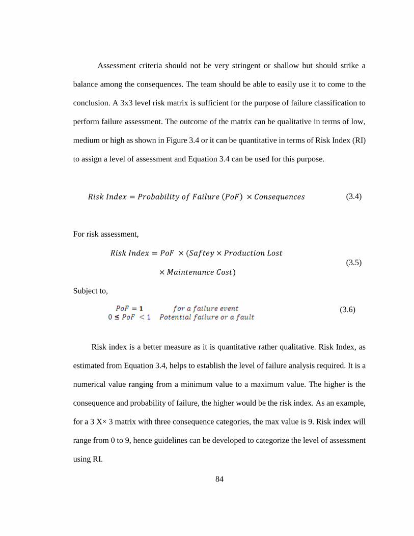
84
Assessment criteria should not be very stringent or shallow but should strike a
balance among the consequences. The team should be able to easily use it to come to the
conclusion. A 3x3 level risk matrix is sufficient for the purpose of failure classification to
perform failure assessment. The outcome of the matrix can be qualitative in terms of low,
medium or high as shown in Figure 3.4 or it can be quantitative in terms of Risk Index (RI)
to assign a level of assessment and Equation 3.4 can be used for this purpose.
𝑅𝑖𝑠𝑘 𝐼𝑛𝑑𝑒𝑥 = 𝑃𝑟𝑜𝑏𝑎𝑏𝑖𝑙𝑖𝑡𝑦 𝑜𝑓 𝐹𝑎𝑖𝑙𝑢𝑟𝑒 (𝑃𝑜𝐹) × 𝐶𝑜𝑛𝑠𝑒𝑞𝑢𝑒𝑛𝑐𝑒𝑠 (3.4)
For risk assessment,
𝑅𝑖𝑠𝑘 𝐼𝑛𝑑𝑒𝑥 = 𝑃𝑜𝐹 × (𝑆𝑎𝑓𝑡𝑒𝑦 × 𝑃𝑟𝑜𝑑𝑢𝑐𝑡𝑖𝑜𝑛 𝐿𝑜𝑠𝑡
× 𝑀𝑎𝑖𝑛𝑡𝑒𝑛𝑎𝑛𝑐𝑒 𝐶𝑜𝑠𝑡)
(3.5)
Subject to,
(3.6)
Risk index is a better measure as it is quantitative rather qualitative. Risk Index, as
estimated from Equation 3.4, helps to establish the level of failure analysis required. It is a
numerical value ranging from a minimum value to a maximum value. The higher is the
consequence and probability of failure, the higher would be the risk index. As an example,
for a 3 X× 3 matrix with three consequence categories, the max value is 9. Risk index will
range from 0 to 9, hence guidelines can be developed to categorize the level of assessment
using RI.

85
3.1.3 Analysis Phase
In this phase, all the activities related to failure investigation are performed. Most
of the companies have systems or preferred methods in place to conduct formal and
informal investigations. However, not all follow a structured approach for the complete
process. Simple 5-Why approach for simple failures and other complex techniques for
formal investigations can be used. The proposed framework can be effectively used for
both formal and informal investigations. There are three key steps in this phase which focus
on the identification of the root cause(s) and the corrective actions.
3.1.3.1 Develop Historical Timeline
In this step, historical time sequence of the events prior to failure is established
which includes the events and other critical information with data and time as shown in
Figure 3.7. Failure timeline provides extremely useful information and suggests the
changes made during the life of the equipment, from design to operation. This information
is extremely important and the timeline must be factual, precise, and quantified to ensure
its best use.
3.1.3.2 Perform Root Cause Analysis
Root cause analysis is the heart of the proposed framework. After establishing a
failure or fault incident, possible failure modes based on the information are developed and
also the actions or causes that contribute to the failure mode are also developed. At this
stage, all the causes to failure modes are hypothetical before evidence is obtained to support
the real cause of a specific failure mode. All the technical possible failure modes are
86
generally evaluated to ensure thorough investigation. Once all hypotheses are developed,
they are rejected or accepted with the sound engineering knowledge, and facts based on
laboratory test results. If the possible cause cannot be rejected, it should have a
recommendation for it. In general, there are more than one causes of a failure so all the
causes must be supported by well documented evidences and facts. There are some chronic
challenges in this step like stopping too early with multiple root causes, or mistaking a
symptom for a root cause, is very common. In this step, we identify the root cause(s) and
use all the test results, material analysis and information from previous steps to make
decisions.
3.1.3.3 Identify Root Cause(s)
Once the root cause analysis step is complete, the next step is the classification
of the direct and contributing causes. Physical, human and latent causes are classified.
There may be more than one cause of a failure, so it must be ensured that the possible
failures have been explored. Root cause must be supported by factual data and evidences.
This is also a critical step which may lead to repeat failures if the real root cause(s) are not
identified.
3.1.4 Implement and Track Phase
This phase is extremely important for the success of the investigation process, as
the real value of the complete assessment process lies in the implementation of the
recommendations. It is very common in industry to implement the main recommendation
and move on with the operations and ignore or overlook the remaining recommendations.
87
The poor implementation and tracking of recommendations is one of the basic causes of
the repeat failures. In this phase, it is suggested that the recommendations are classified
based on a prioritization matrix. The implementation priority is decided by the fact that
how much a recommendation is contributing in avoidance of the failure. The stronger the
correlation, more chances are that it will get a high priority.
3.1.4.1 Develop Corrective Actions
Proper and effective corrective actions and their implementation is a barrier to
repeat failures or a failure in case of minor fault. Once the root cause(s) are identified,
proper, effective and smart recommendations must be developed. The corrective action
must be specific and open ended recommendations must be avoided. The corrective action
must be technically feasible and should not be an over kill, thereby making the system
over-designed. There are disadvantages of the poor corrective actions which may not be
addressing a root cause and may shift failure to other weaker components or parts of the
system.
3.1.4.2 Prioritize and Implement
There are certain ways to classify recommendations. Critical recommendations
are the ones that have a greater impact on continuous operation and should be implemented
first. Impact and difficulty matrix can be used to classify low hanging fruits. An example
of the modified priority matrix is shown in Figure 3.5 [6].
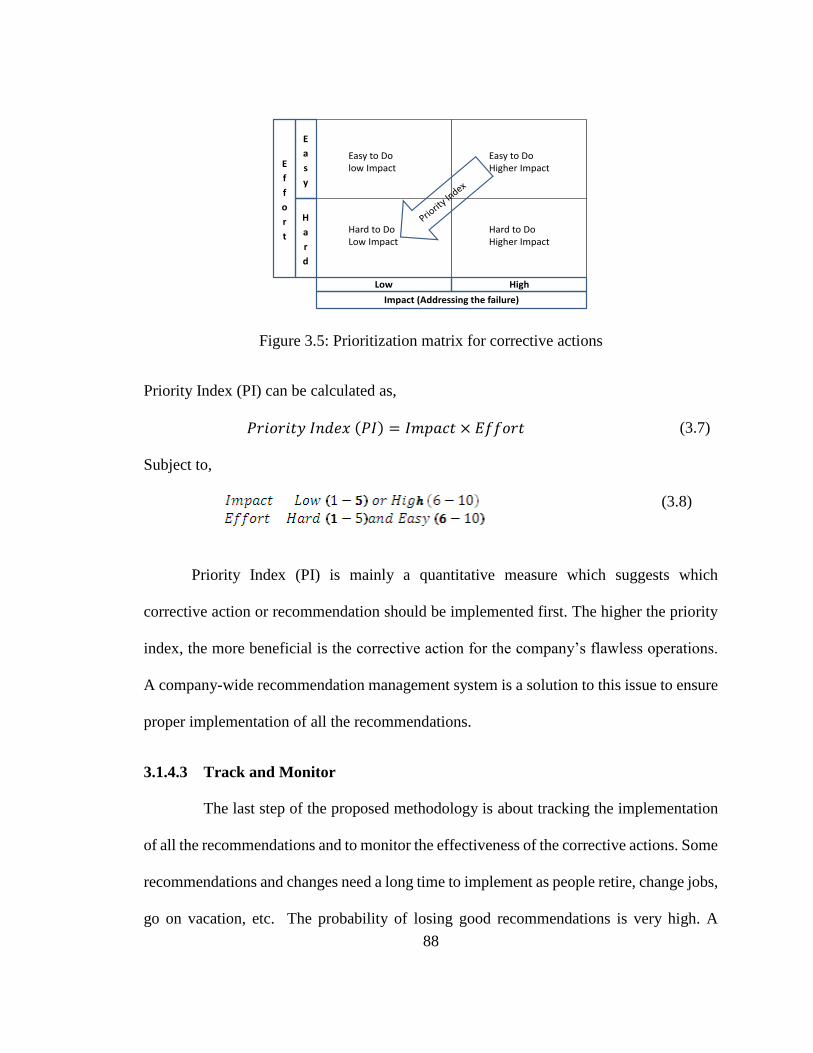
88
Figure 3.5: Prioritization matrix for corrective actions
Priority Index (PI) can be calculated as,
𝑃𝑟𝑖𝑜𝑟𝑖𝑡𝑦 𝐼𝑛𝑑𝑒𝑥 (𝑃𝐼) = 𝐼𝑚𝑝𝑎𝑐𝑡 × 𝐸𝑓𝑓𝑜𝑟𝑡 (3.7)
Subject to,
(3.8)
Priority Index (PI) is mainly a quantitative measure which suggests which
corrective action or recommendation should be implemented first. The higher the priority
index, the more beneficial is the corrective action for the company’s flawless operations.
A company-wide recommendation management system is a solution to this issue to ensure
proper implementation of all the recommendations.
3.1.4.3 Track and Monitor
The last step of the proposed methodology is about tracking the implementation
of all the recommendations and to monitor the effectiveness of the corrective actions. Some
recommendations and changes need a long time to implement as people retire, change jobs,
go on vacation, etc. The probability of losing good recommendations is very high. A
Low High
Easy to DoHigher Impact
Hard to DoHigher Impact
E
a
s
y
H
a
r
d
Easy to Dolow Impact
Hard to DoLow Impact
Impact (Addressing the failure)
E
f
f
o
r
t

89
formal management system is highly recommended. Once all the recommendations are
completed, the investigation should be closed in the system, which tells the team that all
the corrective actions have been implemented. The monitoring feedback mostly uses
performance indicators to evaluate the quality of the investigation and corrective actions.
System availability is a parameter to track and evaluate the quality of the investigation and
the effectiveness of the recommendations.
3.4 Application of Proposed Approach using Case Studies
Equipment fails and failure assessment is performed to identify the root cause(s)
and corrective actions to avoid repeat failures. Failure assessment is also conducted on
faults which may lead to a failure like “near-miss” in safety terminology. So, it is critical
to conduct the fault assessment. In processing facilities, consequences of a failure are
humongous, both financially and in terms of safety. Section 3.4 discusses the two real case
studies to demonstrate the proposed methodology and their impact on system availability.
3.4.1 Case Study: Bearing Failure
In rotating machines like pumps and compressors, bearing is an important
component and is often proactively monitored for proper functionality through predictive
tools. In this case [22], there are two motors driving solvent pumps to supply solvent to a
column, as shown in the schematic in Figure 3.6. These pumps have n+1 redundancy and
are critical to the continuous operation of the plant. In this event, the plant experienced

90
unwanted interruption in production, when both pumping systems failed due to a common
failure mode.
Figure 3.6: Pumping system
The risk-based failure assessment methodology comprising of the four phases, as
described in Section 3.3, was applied and is briefly discussed in the following Section.
3.4.1.1 Plan Phase
Failure assessment process was started with the reporting of the incident in
maintenance management system and failure assessment was requested. Along with failure
report in maintenance management system, the failure mode and the related preliminary
data was recorded. The investigation was assigned to a trained engineer to lead the
assessment. Following step 2 of the plan phase, the site was preserved, and the initial
findings were collected from the field. Along with this activity, preliminary information
via interviews, plant online information system was used to collect the online data like

91
process conditions, equipment datasheet, maintenance history, cross-Sectional drawings,
before setting up an investigation team.
3.4.1.2 Assessments Phase:
Based on the collected information, subject matter experts were invited to
effectively evaluate the failure with the available information. With all the information and
the right people, failure consequence assessment was performed using a consequence
assessment criterion as per Figure 3.4, to identify the scope and level of this investigation.
Risk index suggested that this incident required a formal failure investigation as it involved
a major financial consequence. After the assessment phase, it was concluded a formal
failure investigation be performed.
3.4.1.3 Analysis Phase
The first step in the analysis process was to develop an incident event timeline as
shown in Figure 3.7.
Figure 3.7: Failure event timeline

92
In the event timeline, all the key critical events were captured to understand the
operations and maintenance of the equipment. The transient condition experienced by the
equipment was also captured during the timeline to assess the impact of transients. Once
the timeline was developed, the identified failure was chosen and identification of possible
failure modes was started.
Figure 3.8: Failure cause relationship tree
After selecting the possible failure modes, possible triggers or actions which could
cause the failure mode were developed with the help of expert knowledge and the available
information. After developing these actions, called hypotheses, they were assigned to team
members to work on to accept or reject them, based on the data or engineering experience
supported by theory or the inspection of failed parts or using the material analysis reports
and the results as shown in Figure 3.8 and 3.9. In this case, there was strong evidence of

93
bearing failure supported by the inspection of failed parts and the vibration data as provided
in Figure 3.9 and 3.10. The bearing failure frequency matched with the bearing ball pass
frequency, which is solid evidence that the failure initiated at the bearing balls. The root
causes may be physical, human or latent but accepted propositions should be used to
identify the root causes.
Figure 3.9: Evidence – failed part condition
Figure 3.10: Vibration Trend – overall vibration and bearing frequency
3.4.1.4 Implement and Track Phase:
After identifying the root causes, effective recommendations were developed and
prioritized using a prioritizing matrix. All the recommendations were not critical; some
were critical for the operation of the repaired equipment and some were good to improve
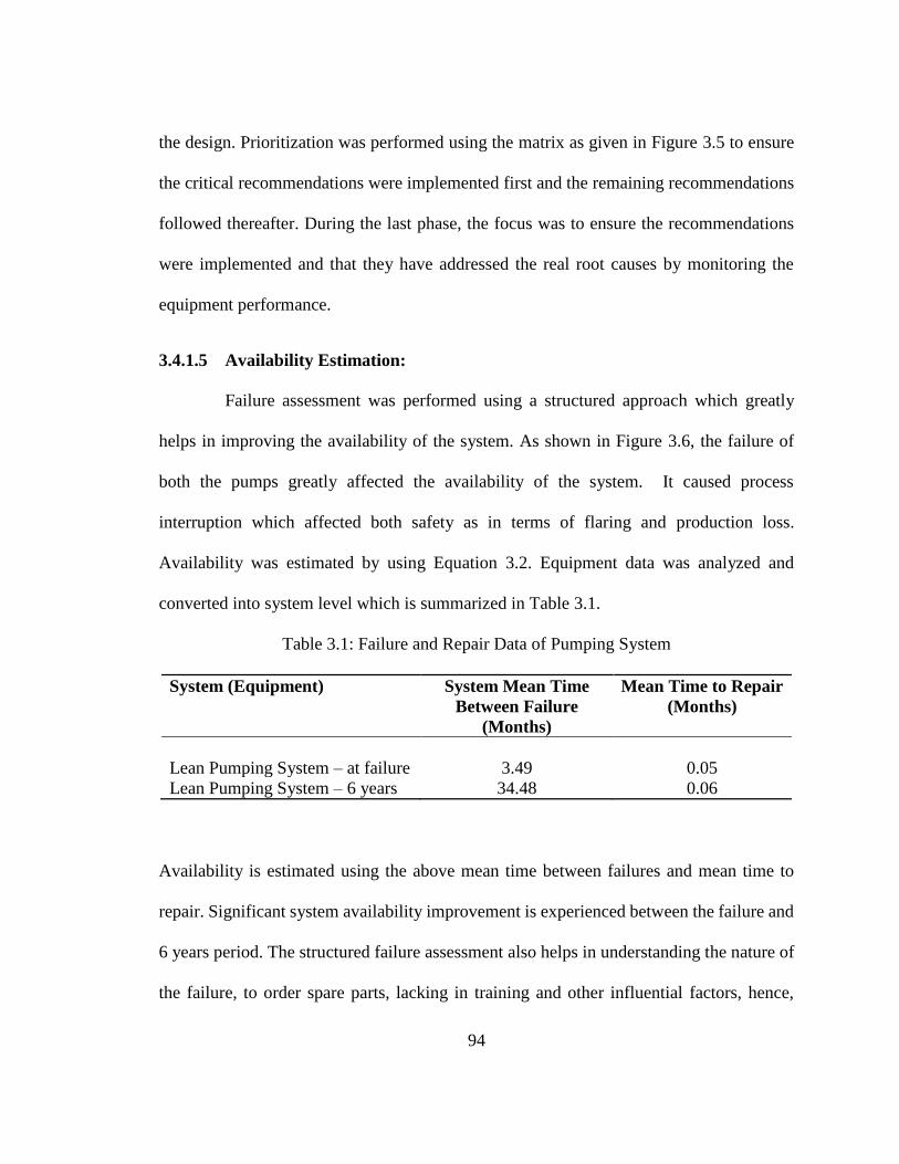
94
the design. Prioritization was performed using the matrix as given in Figure 3.5 to ensure
the critical recommendations were implemented first and the remaining recommendations
followed thereafter. During the last phase, the focus was to ensure the recommendations
were implemented and that they have addressed the real root causes by monitoring the
equipment performance.
3.4.1.5 Availability Estimation:
Failure assessment was performed using a structured approach which greatly
helps in improving the availability of the system. As shown in Figure 3.6, the failure of
both the pumps greatly affected the availability of the system. It caused process
interruption which affected both safety as in terms of flaring and production loss.
Availability was estimated by using Equation 3.2. Equipment data was analyzed and
converted into system level which is summarized in Table 3.1.
Table 3.1: Failure and Repair Data of Pumping System
System (Equipment) System Mean Time
Between Failure
(Months)
Mean Time to Repair
(Months)
Lean Pumping System – at failure 3.49 0.05
Lean Pumping System – 6 years 34.48 0.06
Availability is estimated using the above mean time between failures and mean time to
repair. Significant system availability improvement is experienced between the failure and
6 years period. The structured failure assessment also helps in understanding the nature of
the failure, to order spare parts, lacking in training and other influential factors, hence,
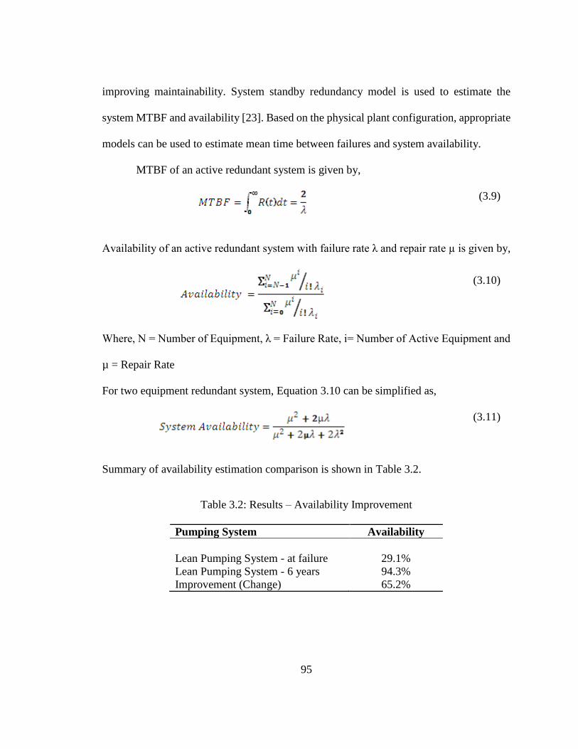
95
improving maintainability. System standby redundancy model is used to estimate the
system MTBF and availability [23]. Based on the physical plant configuration, appropriate
models can be used to estimate mean time between failures and system availability.
MTBF of an active redundant system is given by,
(3.9)
Availability of an active redundant system with failure rate λ and repair rate µ is given by,
(3.10)
Where, N = Number of Equipment, λ = Failure Rate, i= Number of Active Equipment and
µ = Repair Rate
For two equipment redundant system, Equation 3.10 can be simplified as,
(3.11)
Summary of availability estimation comparison is shown in Table 3.2.
Table 3.2: Results – Availability Improvement
Pumping System Availability
Lean Pumping System - at failure 29.1%
Lean Pumping System - 6 years 94.3%
Improvement (Change) 65.2%

96
3.4.1.6 Results
True identification of the failure causes along with their corrective action
implementation greatly expands the availability and reliability of the equipment.
Availability is improved by 65.2% points whereas significant improvement in MTBF is
also realized using the proposed risk-based approach. The structured process helps
developing the confidence of the team by using a consistent and structured proposed
methodology. This structured failure assessment approach also helps in identifying the
other underlying issues during investigation i.e., system maintainability, critical parts
required to improve maintainability and other latent issues of training and procedures.
3.4.2 Case Study: Drive Coupling Failure
Coupling is an essential component of rotating machinery. The main function of
a coupling is to transmit torque to drive equipment from a driver and compensate for slight
misalignments. Misalignment can be due to installation error or limitations and operating
conditions. The failure of a coupling means failure of the system. The proposed approach
was used to investigate the failure of the coupling. The methodology suggested in Figure
3.3 was used for identification of root cause(s), manage recommendations and estimate the
availability enhancement. The system configuration is given in Figure 3.11. The system
consisted of 5 centrifugal pumps where 4 out of the 5 were required to operate the system
at 100% load.
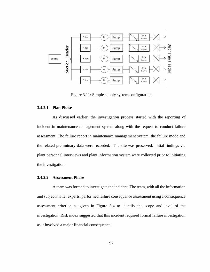
97
Figure 3.11: Simple supply system configuration
3.4.2.1 Plan Phase
As discussed earlier, the investigation process started with the reporting of
incident in maintenance management system along with the request to conduct failure
assessment. The failure report in maintenance management system, the failure mode and
the related preliminary data were recorded. The site was preserved, initial findings via
plant personnel interviews and plant information system were collected prior to initiating
the investigation.
3.4.2.2 Assessment Phase
A team was formed to investigate the incident. The team, with all the information
and subject matter experts, performed failure consequence assessment using a consequence
assessment criterion as given in Figure 3.4 to identify the scope and level of the
investigation. Risk index suggested that this incident required formal failure investigation
as it involved a major financial consequence.
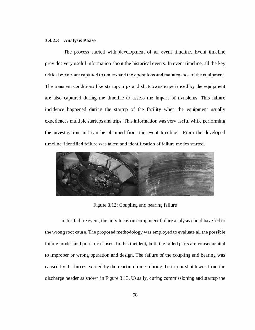
98
3.4.2.3 Analysis Phase
The process started with development of an event timeline. Event timeline
provides very useful information about the historical events. In event timeline, all the key
critical events are captured to understand the operations and maintenance of the equipment.
The transient conditions like startup, trips and shutdowns experienced by the equipment
are also captured during the timeline to assess the impact of transients. This failure
incidence happened during the startup of the facility when the equipment usually
experiences multiple startups and trips. This information was very useful while performing
the investigation and can be obtained from the event timeline. From the developed
timeline, identified failure was taken and identification of failure modes started.
Figure 3.12: Coupling and bearing failure
In this failure event, the only focus on component failure analysis could have led to
the wrong root cause. The proposed methodology was employed to evaluate all the possible
failure modes and possible causes. In this incident, both the failed parts are consequential
to improper or wrong operation and design. The failure of the coupling and bearing was
caused by the forces exerted by the reaction forces during the trip or shutdowns from the
discharge header as shown in Figure 3.13. Usually, during commissioning and startup the
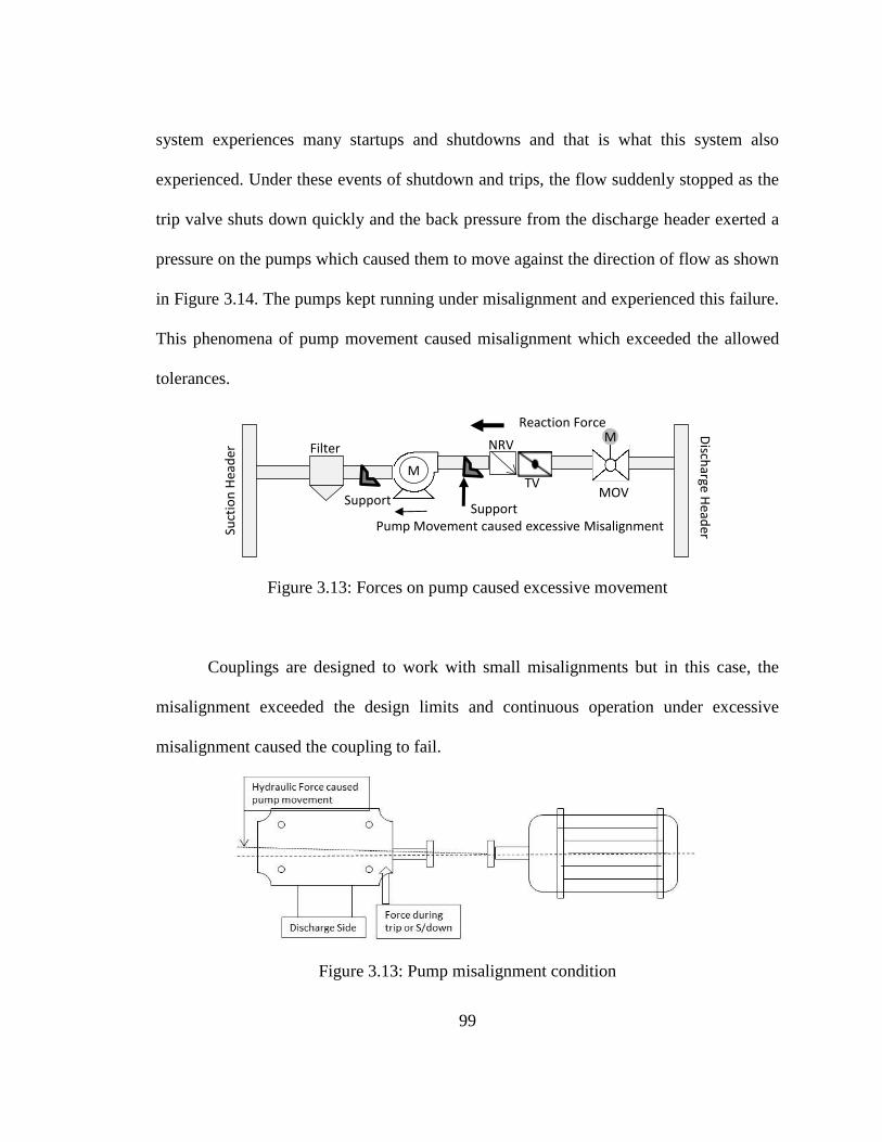
99
system experiences many startups and shutdowns and that is what this system also
experienced. Under these events of shutdown and trips, the flow suddenly stopped as the
trip valve shuts down quickly and the back pressure from the discharge header exerted a
pressure on the pumps which caused them to move against the direction of flow as shown
in Figure 3.14. The pumps kept running under misalignment and experienced this failure.
This phenomena of pump movement caused misalignment which exceeded the allowed
tolerances.
Figure 3.13: Forces on pump caused excessive movement
Couplings are designed to work with small misalignments but in this case, the
misalignment exceeded the design limits and continuous operation under excessive
misalignment caused the coupling to fail.
Figure 3.13: Pump misalignment condition
M
M
Filter
Support
NRV
MOVTV
Suct
ion
Hea
der
Disch
arge Head
er
SupportPump Movement caused excessive Misalignment
Reaction Force
100
A support system was available to counteract the hydraulic forces in case of trips
and shutdown but was found broken. This supported the fact that the reaction forces were
higher than the design strength. All the measurements and component analysis was done
to ensure the wrong operation and insufficient design were the causes that contributed to
this event.
3.4.2.4 Implement and Track Phase
After identifying the root causes, recommendations were developed and
prioritized using a prioritizing matrix as shown in Figure 3.5. The prioritization matrix
helped in selecting the critical recommendations which were implemented first, before the
less important corrective actions. As a corrective action in this case, the operating
philosophy was changed, improvement in the strength of the supports along with other
recommendations. During the last phase, the attention is to ensure that the
recommendations have been implemented and they have addressed the real root cause by
monitoring the equipment performance during tracking. In the last, estimated the
availability and failure rate to ensure root cause was correctly found and the right corrective
action were developed and implemented.
3.4.2.5 Availability Estimation:
A structured approach has proven to be a great tool in enhancing availability of
the system. As shown in Figure 3.12, the failure of multiple pumps greatly affected the
availability and reliability of the system and caused process interruption and production
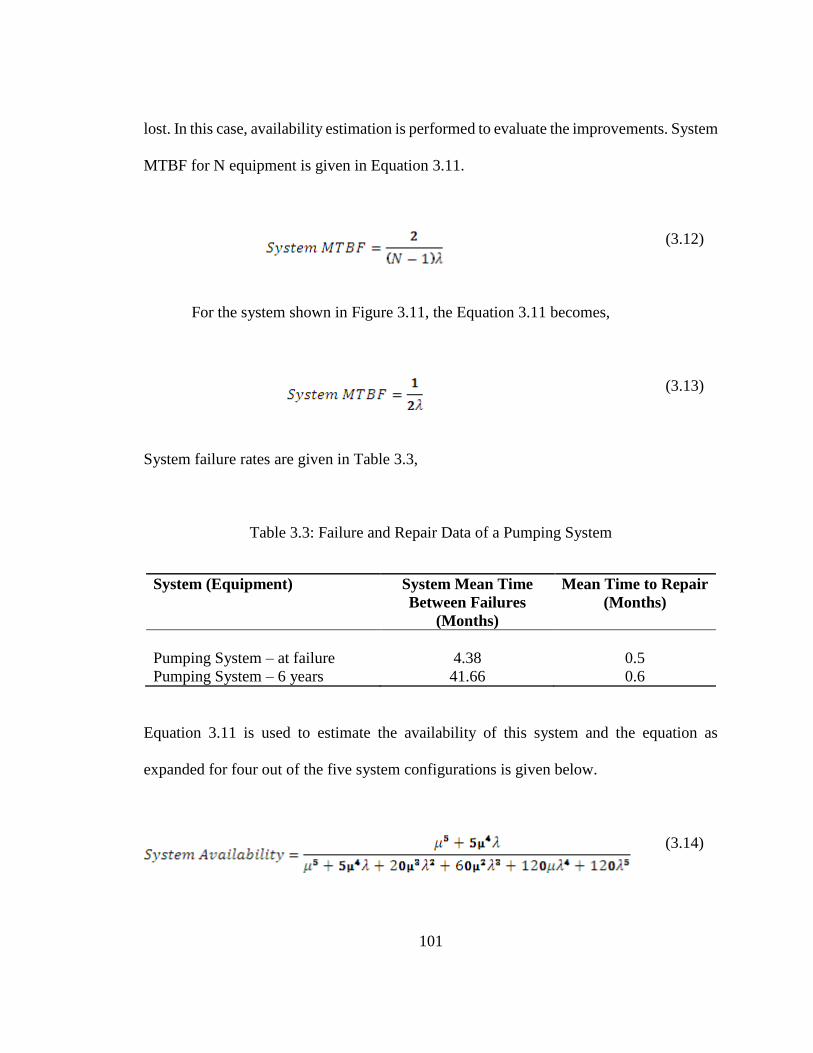
101
lost. In this case, availability estimation is performed to evaluate the improvements. System
MTBF for N equipment is given in Equation 3.11.
(3.12)
For the system shown in Figure 3.11, the Equation 3.11 becomes,
(3.13)
System failure rates are given in Table 3.3,
Table 3.3: Failure and Repair Data of a Pumping System
System (Equipment) System Mean Time
Between Failures
(Months)
Mean Time to Repair
(Months)
Pumping System – at failure 4.38 0.5
Pumping System – 6 years 41.66 0.6
Equation 3.11 is used to estimate the availability of this system and the equation as
expanded for four out of the five system configurations is given below.
(3.14)
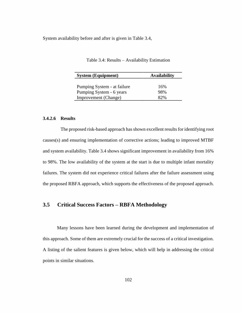
102
System availability before and after is given in Table 3.4,
Table 3.4: Results – Availability Estimation
System (Equipment) Availability
Pumping System - at failure 16%
Pumping System - 6 years 98%
Improvement (Change) 82%
3.4.2.6 Results
The proposed risk-based approach has shown excellent results for identifying root
causes(s) and ensuring implementation of corrective actions; leading to improved MTBF
and system availability. Table 3.4 shows significant improvement in availability from 16%
to 98%. The low availability of the system at the start is due to multiple infant mortality
failures. The system did not experience critical failures after the failure assessment using
the proposed RBFA approach, which supports the effectiveness of the proposed approach.
3.5 Critical Success Factors – RBFA Methodology
Many lessons have been learned during the development and implementation of
this approach. Some of them are extremely crucial for the success of a critical investigation.
A listing of the salient features is given below, which will help in addressing the critical
points in similar situations.

103
1. The proposed process must be followed: A proper understanding of the structured
process is required.
2. Communication: A proper communication platform should be available to ensure
that the cross-functional team has proper and timely information.
3. Team members: The team leader must be properly trained on the methodology and
other facilitation techniques. Other team members must be knowledgeable and
skilled in the area of the investigation.
4. Tracking and implementation: Experience has shown that most of the repeat
failures are the result of a lack of implementation of the recommendations or
corrective actions. A suitable and traceable recommendation management system
should be developed.
5. Recognition: Team efforts should be appreciated by management to ensure team
motivation and development of a proactive reliability culture in the organization.
3.6 Conclusion
The proposed risk-based failure assessment methodology has shown far-reaching
improvements in handling equipment fault and failures to enhance safety and availability.
Risk-based quantitative analysis to identify the level of root cause analysis and corrective
action prioritization is extremely effective and efficient. The proposed method can be
equally applied on potential failures and faults to proactively address the potential failure;
104
greatly reducing the maintenance costs and loss production events. Learning of an
assessment can be shared and applied to other similar equipment, which can optimize the
maintenance and maintainability. Highly encouraging results have been accomplished
from the implementation of the proposed framework. In this work, the presented cases have
shown great improvements in system availability; 65.2% in case 1 and 82% in case 2. The
proposed approach is user friendly and can be used by following the step by step process.
A software solution will greatly enhance the efficiency of the failure assessment process
along with the other benefits of data structuring and availability. There are other methods
that complement improvements in availability; but the proposed risk-based approach
suggests an optimal and effective solution to a general industry problem of repeat failures
and faults.
105
CHAPTER 4
SYSTEM AVAILABILITY ENHANCEMENT USING DECISION
TREES 4
Abstract
System availability is a key performance measure in the process industry. It ensures
continuous operation of facilities to meet production targets, personnel safety and
environmental sustainability. Process machinery condition assessment, early fault
detection and its management are vital elements to assure overall system availability. These
elements can be explored and managed effectively by extracting hidden knowledge from
machinery vibration information to improve plant availability and safe operations.
4 This Chapter is based on the published work in a peer-reviewed journal. Qadeer Ahmed, Fatai
A. Anifowose, Faisal Khan (2015), “System Availability Enhancement using Computational
Intelligence based Decision Tree Predictive Model,” Accepted in Journal of Risk and Reliability
Engineering. To minimize the duplication, all the references are listed in the reference list. The
contribution of the authors is presented in Section titled, “Co-authorship Statement”.

106
This Chapter describes a Decision Tree (DT) based computational intelligence
model using machinery vibration data to detect machinery faults, their severity, and
suggests appropriate actions to avoid unscheduled failures. Vibration data for this work
were collected using a machinery simulator and real-world machine to show the
applicability of the proposed model. Later, the data was analyzed to detect faults using DT
based model that was developed in MATLAB. Fault detection classification accuracies of
98% during training and 93% during testing showed excellent performance of the proposed
model. The suggested model also revealed that the proposed formulation has capability of
detecting faults correctly in the range of 98% to 99%. The results highlight that the
suggested predictive decision tree based model is effective in evaluating the condition of
process machinery and predicting unscheduled equipment breakdowns with better
accuracy and with reduced human effort.
4.1 Introduction
Early fault detection and management (FDM) are two main aspects of successful
and continuous plant operations at low cost. Computational intelligence and technological
advancements have provided us a platform to develop intelligent systems where machinery
vibration data and process information can be used for assessing equipment health.
Equipment vibration and process information have proven to be very effective in
performing fault diagnostics and prognostics to improve the overall availability, reliability
and maintainability of complex operating systems. Proper analysis of vibration signals is

107
an important tool that enables engineers to timely detect and identify faults to avoid system
failures. Although faults and failures are synonymously used in industry but they represent
different equipment conditions. In simple terms, a fault is a state where the equipment is
functional but with degraded performance or does not function properly when required [1].
A failure is described as a condition where the equipment fails to perform its defined
function and is in a state of a complete breakdown [2]. To avoid failures and keep repair
costs in control, faults should be detected and managed efficiently during their infancy
stage. Proper maintenance action helps in managing faults to avoid failures, which usually
costs three to four times higher than a planned repair cost [3]. Presently, vibration data are
usually collected during routine maintenance and analyzed by operators to assess the
condition of equipment. This assessment is very much dependent upon the skill level of
the operator and any wrong interpretation can have negative consequences. Early and
correct detection of faults and its management help improving availability by addressing
both dependencies of availability, i.e. reliability and maintainability as presented in
Equation 4.1.
𝐴𝑣𝑎𝑖𝑙𝑎𝑏𝑖𝑙𝑖𝑡𝑦 =𝑅𝑒𝑙𝑖𝑎𝑏𝑖𝑙𝑖𝑡𝑦 (𝑀𝑇𝐵𝐹)
𝑅𝑒𝑙𝑖𝑎𝑏𝑖𝑙𝑖𝑡𝑦 (𝑀𝑇𝐵𝐹) + 𝑀𝑎𝑖𝑛𝑡𝑎𝑖𝑛𝑎𝑏𝑖𝑙𝑖𝑡𝑦 (𝑀𝑇𝑇𝑅) (4.1)
where, MTBF = Mean time between failures and MTTR = Mean time to repair.
Equipment condition, maintenance cost, operating time and overall risk are
interrelated as shown in Figure 4.1. In this figure, the x-axis represents the operating time

108
and the y-axis represents the equipment condition and influence of cost. The 𝐶1 range
represents the equipment with minor signs of degradation; the 𝐶2 range shows the signs of
some damage; and 𝐶3 is the condition where the condition is worst and major action is
required. 𝐹 is a point where the equipment failed to perform its function and is classified
as a point of failure or potential failure. Overall risk of a failure includes failure cost,
environmental impact along with personnel safety and production loses. If a fault is
detected in zone 𝐶1, the cost and risk would be significantly less compared to the fault that
is identified in zone 𝐶3. Early fault detection can be effectively addressed by a normal
maintenance action like greasing and tightening of bolts. A fault in the advanced stage
would require component replacement and higher repair cost. Due to these benefits, cost
avoidance and improvement in plant availability, equipment condition monitoring is
gaining significant importance. The outcome of equipment condition based on past history
is classified as diagnostics while the prediction of remaining equipment life is generally
termed as prognostics, as presented in Figure 4.1. This work mainly focuses toward the
fault diagnosis and its management rather than the prediction of remaining useful life.

109
Figure 4.1: Diagnostic-prognostic concept with equipment condition, risk and cost
Machines are complex systems and usually exhibit many faults, however, this
research focuses on two faults and they are: unbalance and misalignment. Unbalance is
defined as “a condition when the center-of-gravity of the rotor is out of alignment with its
axis-of-rotation” [4]. Misalignment is defined as “a condition when relative center lines of
shaft of two machines are not in line with each other” [5]. These two faults are top
contributors to machine diagnostic processes and among 90% of the reported faults in
machinery failures [6]. Vibration data in fault detection is extremely helpful as a fault in a
machine can be represented by frequency components and their severity by signal
amplitude. Figure 4.2 shows the general spectrum of the unbalance and misalignment
where good understanding of spectrum, component frequencies and signal amplitude limits
greatly helps in fault detection.

110
Figure 4.2: Spectrum snapshot of misalignment and unbalance
Presently, fault diagnosis is carried out using different condition monitoring
techniques, i.e. oil condition monitoring, vibration and other process parameters
monitoring. These methods are prone to human errors, excessive man-hours, and are
sometimes inaccurate due to the misunderstanding of the correlation of these parameters
for a single output. To ensure effective prediction and generalization, all known possible
machine conditions and fault scenarios should have representation in the training data. To
address this limitation, suggested model formulation is dynamic and easily updated to
allow the addition of new possible scenarios without having to re-model from the scratch.
Second, it is based on the machine learning paradigm rather than the conventional
statistical interpolations, due to these reasons, its improved and robust performance is
guaranteed. The proposed computational intelligence based holistic fault diagnostic and
management scheme methodology utilizes machinery and simulator data to predict faults,
their severity using decision tree (DT) algorithms

111
Computational intelligence through data mining offers promising methods to
extract hidden information patterns from these datasets, which are extremely difficult to
discover with simple statistical analysis. These hidden patterns can be explored and used
to predict some future trends with good quality data. Data mining can be done using
different techniques. Some of the most popular methods are: classification, clustering,
deviation detection and estimation etc. We are focused on classification as we predict using
a pre-labeled classified condition; i.e., machinery unbalance and misalignment.
Classification is a robust method for predicting the illustration class from pre-labeled
instances. Classification is an important task in data mining where a classifier is built based
on some attributes to describe the objects or one attribute to describe the group of the
objects. Later, the classifier is used to predict the group attributes of other cases [7].
The remainder of the Chapter is organized as follows: Section 4.2 discusses the present
state of literature and the work performed in the field of fault diagnostics using smart
algorithms. Section 4.3 provides the formulation of the proposed fault detection model and
fault management strategy. Section 4.4 describes the detailed research methodology
including data collection, experimental setup, the criteria used to evaluate the performance
of the model and the validation of the model with real operational data. Section 4.5 presents
the results with discussion. Conclusions and the contributions are highlighted in Section
4.6.

112
4.2 Literature Review
Fault diagnostics using condition monitoring has become an area of great interest
in industry. The capability of detecting an early fault enables engineers and operators to
reduce the probability of damage and loss. Faults, if not addressed properly can have
catastrophic consequences in terms of lost production, maintenance costs and safety. Due
to these reasons, a number of data mining and optimization techniques have been applied
to fault classification, diagnostics and its management [8-14]. We have explored a holistic
data-driven model, where the focus is on detection and management of faults. In data
driven modeling approach, the available data is generally used to learn hidden patterns and
extract knowledge to detect faults. Academic and industry researchers in the field of
artificial intelligence, pattern recognition, and data mining have considered DTs as an
effective technique. This is one of the reasons for exploring DT for the problem at hand.
Many researchers have used artificial intelligence algorithms to detect machinery faults
and some of them are discussed in this Section. Support vector machine (SVM) models (c-
SVC and nu-SVC) with four kernel functions were used for classification of faults using
statistical features extracted from vibration signals under good and faulty conditions of
rotational mechanical system [15]. A DT algorithm was used to select the prominent
features. These features were given as inputs for training and testing the c-SVC and nu-
SVC model of SVM and their fault classification accuracies were compared. We are
targeting a simpler model compared to hybrid DT-SVM model but with improved, or at
least competitive, detection accuracy. In another work, DT was used for fault detection in

113
bearings using sound signal [16]. Data was collected from the near-field area from good
and faulty bearings with classification accuracy in the range of 68.8 - 95.5%. To detect
motor faults, DTs were also used in another work [17]. A layered dynamic hybrid fault
modeling and extended evolutionary game theory was proposed for reliability,
survivability and fault tolerance analysis [18]. Due to the complexity of the model, the
authors recommended development and implementation of a software program. The DT
model of this work ensures simplicity of implementation with good accuracy. Risk is an
important aspect to evaluate the consequences of certain faults or failures in complex
systems. The operation of such complex systems involves multiple hazards and
consequences in case of breakdown. This makes the area of risk assessment and
quantification extremely important and related to fault detection and management,
availability and maintenance of the systems. To study the relationship between risk,
availability and its consequences in certain scenarios, a risk-based availability analysis
model is presented [19].
As discussed above, fault diagnostics and prognostics through monitoring condition
data have merits. Some of these fault diagnostics techniques are explored further to express
the novelty of this work. A DT-based formulation is developed to identify the causes of the
abnormal vibration [20]. This work mainly focused on automating the vibration diagnosis
process for rotating machinery, which is applicable to vibration diagnosis expert system
rather than detecting faults. Fault diagnosis using DTs is carried out using vibration signals
from a gear box [21]. Features were extracted from vibration data and important features
were used to develop a classification model using a DT algorithm. This work is more

114
focused on helical gear application and general abnormality detection rather than finding
specific faults. In another work, vibration signals from a bearing are used to collect
condition data and develop a pattern to establish conditions [22]. The statistical features
are extracted from vibration signals and representative features that discriminate the
different fault conditions of the bearing are selected using a DT. A rule set is formed from
the extracted features and input to a fuzzy classifier based on intuition and domain
knowledge. Later, the fuzzy classifier is developed and successfully tested. Fault
diagnostics has gained momentum and the latest technologies have been adopted to detect
faults. In [23], data mining is used for fault diagnostic where DT-based principal
component analysis is proposed. Principal component analysis is used to extract features
and a C4.5 algorithm is used for training. A laboratory simulator was used to simulate faults
such as unbalance, shaft cracks, etc. The results show that DT-based principal component
analysis is a better method compared to other advance methods such as back-propagation
neural networks. In another work, bearing defects in rotating machines is explored by
identifying expert rules [24]. Data are collected from vibration signals measured in an
experimental setup to determine statistical parameters. The DT is then constructed by
applying a C4.5 algorithm on the dataset, and so expert rules are established to detect faults.
DTs have been used in a number of previous studies but ours is more rigorous and
exploratory as we considered and implemented a number of innovative approaches to the
machine-learning based modeling paradigm. These mainly include:

115
i. Using a stratified sampling methodology to ensures that each data sample has
an equal chance of being selected for training or validation which allows a good
mix of representative data samples.
ii. In addition to condition monitoring and prediction, our methodology includes
the prediction of the levels of the severity of the machine conditions and how
to manage the fault condition.
iii. The data sets used were obtained from a rigorous experimental procedures and
real machine operating scenarios therefore, more comprehensive and better
representation of real machine fault and operating conditions.
The presented work consists of a fault and its severity assessment. Later, the fault
management strategy is implemented that addresses the handling of detected fault
condition, efficiently, which is indeed a requirement while working in real plant situations.
4.3 Proposed Fault Detection and Management Framework
A health assessment for equipment mainly depends on an effective fault diagnostics
and management process. In this work, identification of a fault, its location and severity is
mainly a diagnostic activity and estimation of a condition based on the severity of the fault,
along with its impact on the operating system, is part of the fault management task. The
proposed framework has three main steps: fault detection, fault severity, and management
116
of faults through proper maintenance action. Maintenance actions depend mostly on the
severity of the fault, which is established by comparing the fault severity with
internationally developed machinery vibration limits. Most failures of rotating equipment
appear in a vibration spectrum by some frequencies, and the severity depends on the level
of amplitude. Many common machinery faults have a strong relationship with running
speed and two important speed factors are unbalance and misalignment, which have been
focused in this Chapter. We classify fault severity risk into three categories: low
(acceptable), medium (caution) and high (dangerous). The low fault level suggests a
machine that can be used continuously with monitoring; medium or caution is a level where
it is required to perform some extra monitoring to track the condition of the equipment.
The last level is for a high or dangerous condition where the machine must be stopped
promptly to avoid a catastrophic failure and a proper investigation shall be performed prior
to another startup. The effective usage of the proposed model, as shown in Figure 4.3, will
help to avoid catastrophic failures, and therefore improving the availability of the systems
in a plant. The proposed framework mainly has three distinct steps, which are discussed in
the following Sections.
4.3.1 Fault Detection
In this step, data are acquired along with feature selection. The feature or variable
must be carefully selected during model development as the accuracy of classification is
greatly dependent upon the right features being considered. Once the features are finalized,
we need to categorize the collected data in faults by assigning labels. Data stratification is

117
performed to ensure a good mix of data without any bias. The data are then used in the
development of a DT model that provides the results in the form of training, and testing
accuracy of the model and its capability of detecting faults.
Figure 4.3: Fault detection and management framework

118
4.3.1.1 Decision Trees in Fault Detection
Decision trees are widely used in many real-life applications, which include
control systems, biomedical engineering, object recognition, power systems and many
more applications. Decision trees are based on the rules, which depend on human
experiences, as well as machinery behavior, which makes it widely used and accepted in
fault detection. DTs have other advantages such as simplicity in design and accurate
prediction [25]. They are also relatively faster in execution compared to other classification
models. In classification models, feature selection is an important process as the accuracy
of the outcome is highly dependent on the relativity of the feature with the problem being
analyzed. Therefore, to ensure optimal solutions, only the best features must be used. We
have tackled the problem uniquely, where a DT algorithm is used to detect machinery faults
along with the severity of the fault. The construction of the DT is based on a training set,
𝑆, which is a set of different experiments. Each experiment or condition specifies the values
for a collection of attributes and for a class. Let the classes be denoted by 𝐶𝑖. There exist
experiments with 𝑛 outcomes that partition the training set 𝐾 into subsets 𝐾𝑖…𝑛. Assume
that 𝑆 is a set of cases, f𝑟𝑒𝑞 (𝐶𝑖, 𝑆) is the number of cases in S that belong to class 𝐶𝑖, and
|𝑆| is the number of cases in set 𝑆. If we select a case at random from set 𝑆 and assume its
relationship with class𝐶𝑖, probability can be computed as,
𝑓𝑟𝑒𝑞 (𝐶𝑖 ,𝑆
|𝑆|) (4.2)
and the information it provides is,
− 𝑙𝑜𝑔2 {𝑓𝑟𝑒𝑞 (𝐶𝑖,𝑆
|𝑆|)} (4.3)

119
The information required to establish a class of an experiment in 𝑆 is given in Equation
4.4. The procedure for designing a DT model follows the steps described below:
Step 1: Calculate 𝐼𝑛𝑓𝑜(𝑆) to identify the class in the training set 𝑆.
𝐼𝑛𝑓𝑜(𝑆) = − ∑ [{𝑓𝑟𝑒𝑞 (𝐶𝑖,𝑆
|𝑆|)} 𝑙𝑜𝑔2 {𝑓𝑟𝑒𝑞 (𝐶𝑖,
𝑆
|𝑆|)}]
𝐾
𝑖=1
(4.4)
where |𝑆| is the number of cases in the training set; 𝐶𝑖 is a class; I = 1,2,3, … ; 𝐾 is the
number of classes; and 𝑓𝑟𝑒𝑞(𝐶𝑖, 𝑆) is the number of cases.
Step 2: Calculate the expected information value, 𝑖𝑛𝑓𝑜𝑋(𝑆) for test 𝑋 to partition samples
in 𝑆.
𝐼𝑛𝑓𝑜𝑋(𝑆) = − ∑ [(|𝑆𝑖|
|𝑆|) 𝐼𝑛𝑓𝑜(𝑆𝑖)]
𝐾
𝑖=1
(4.5)
where 𝐾 is the number of outputs for test, 𝑋, 𝑆𝑖 is a subset of 𝑆 corresponding to 𝑖𝑡ℎ output
and is the number of cases of subset 𝑆𝑖.
Step 3: Calculate the information gain,
𝐺𝑎𝑖𝑛(𝑋) = 𝐼𝑛𝑓𝑜(𝑆) − 𝐼𝑛𝑓𝑜𝑋(𝑆) (4.6)
𝐺𝑎𝑖𝑛(𝑋) = − ∑ [{𝑓𝑟𝑒𝑞 (𝐶𝑖,𝑆
|𝑆|)} 𝑙𝑜𝑔2 {𝑓𝑟𝑒𝑞 (𝐶𝑖,
𝑆
|𝑆|)}]
𝐾
𝑖=1
+ ∑ [(|𝑆𝑖|
|𝑆|) 𝐼𝑛𝑓𝑜(𝑆𝑖)]
𝐾
𝑖=1
(4.7)

120
Step 4: Calculate the partition information value 𝑆𝑝𝑙𝑖𝑡𝑖𝑛𝑓𝑜(𝑋) acquiring for 𝑆,
partitioned into 𝐿 subsets,
𝑆𝑝𝑙𝑖𝑡𝐼𝑛𝑓𝑜(𝑋) = −1
2 ∑ [
|𝑆𝑖|
|𝑆|𝑙𝑜𝑔2
|𝑆𝑖|
|𝑆|+ (1 −
|𝑆𝑖|
|𝑆|) 𝑙𝑜𝑔2(1
𝐿
𝑖=1
−|𝑆𝑖|
|𝑆|)]
(4.8)
Step 5: Classification tree splits nodes based on either impurity or node error [26]. There
are three general arguments to split the node and they are:
i. Gini’s Diversity Index: The Gini index of a node is given by:
𝐺𝑖𝑛𝑖 𝐼𝑛𝑑𝑒𝑥 = 1 − ∑ 𝑝2(𝑖)
𝑖
(4.9)
where the sum is over the classes 𝑖 at a node, and 𝑝(𝑖) is the observed fraction of classes
with class 𝑖 that reaches the node. A node with one class has index 0, otherwise any positive
value.
ii. Deviance Diversity Index: The deviance of a node is given by:
𝐷𝑒𝑣𝑖𝑎𝑛𝑐𝑒 = − ∑ 𝑝(𝑖)𝑙𝑜𝑔𝑝(𝑖)
𝑖
(4.10)
where the sum is over the classes 𝑖 at a node, and 𝑝(𝑖)is the observed fraction of classes
with class 𝑖 that reaches the node. A pure node has deviance 0, otherwise it is positive.
iii. Twoing Index: It is not a purity measure but a different way to split a node. The
Twoing function is given by:
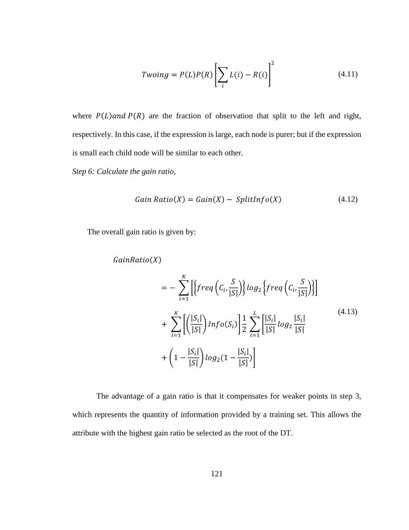
121
𝑇𝑤𝑜𝑖𝑛𝑔 = 𝑃(𝐿)𝑃(𝑅) [∑ 𝐿(𝑖)
𝑖
− 𝑅(𝑖)]
2
(4.11)
where 𝑃(𝐿)𝑎𝑛𝑑 𝑃(𝑅) are the fraction of observation that split to the left and right,
respectively. In this case, if the expression is large, each node is purer; but if the expression
is small each child node will be similar to each other.
Step 6: Calculate the gain ratio,
𝐺𝑎𝑖𝑛 𝑅𝑎𝑡𝑖𝑜(𝑋) = 𝐺𝑎𝑖𝑛(𝑋) − 𝑆𝑝𝑙𝑖𝑡𝐼𝑛𝑓𝑜(𝑋) (4.12)
The overall gain ratio is given by:
𝐺𝑎𝑖𝑛𝑅𝑎𝑡𝑖𝑜(𝑋)
= − ∑ [{𝑓𝑟𝑒𝑞 (𝐶𝑖 ,𝑆
|𝑆|)} 𝑙𝑜𝑔2 {𝑓𝑟𝑒𝑞 (𝐶𝑖,
𝑆
|𝑆|)}]
𝐾
𝑖=1
+ ∑ [(|𝑆𝑖|
|𝑆|) 𝐼𝑛𝑓𝑜(𝑆𝑖)]
𝐾
𝑖=1
1
2 ∑ [
|𝑆𝑖|
|𝑆|𝑙𝑜𝑔2
|𝑆𝑖|
|𝑆|
𝐿
𝑖=1
+ (1 −|𝑆𝑖|
|𝑆|) 𝑙𝑜𝑔2(1 −
|𝑆𝑖|
|𝑆|)]
(4.13)
The advantage of a gain ratio is that it compensates for weaker points in step 3,
which represents the quantity of information provided by a training set. This allows the
attribute with the highest gain ratio be selected as the root of the DT.

122
4.3.2 Fault Severity
All the faults in a system have different importance and that was the reason we
have chosen to collect the data with a known severity condition, which was used in training
and testing. In other words, we have implanted the severity in the fault data during the
experiment design. Table 4.2 represents all the tests with different faults and their severity
conditions.
4.3.3 Fault Management Strategy
The last part of the proposed approach is fault management, which can only be
performed once the fault is detected and its severity is established. The action is mainly
dependent on the severity of the fault. If the fault is in the low risk category, continuous
monitoring can help to ensure that any further development of the fault is quickly
identified. Such faults may actually not be a real fault but the machine’s inherent response
at that operating level. Later, if the trend increases along with the amplitude of the
vibration, it has to be investigated properly using both frequency and time domains to
understand the fault. Faults can be investigated using spectrum as certain frequencies in
machines represent certain components in machines. The bearing frequencies, gear
frequencies, unbalance conditions, and misalignment conditions can be detected using
spectrums. Lastly, if a machine experiences very high vibration levels and reaches the
reference limits of vibration monitoring standards or other experienced based levels, it must
be stopped properly and a detailed root cause failure investigation must be performed to
understand the underlying reason of the faults. There are many reference standards
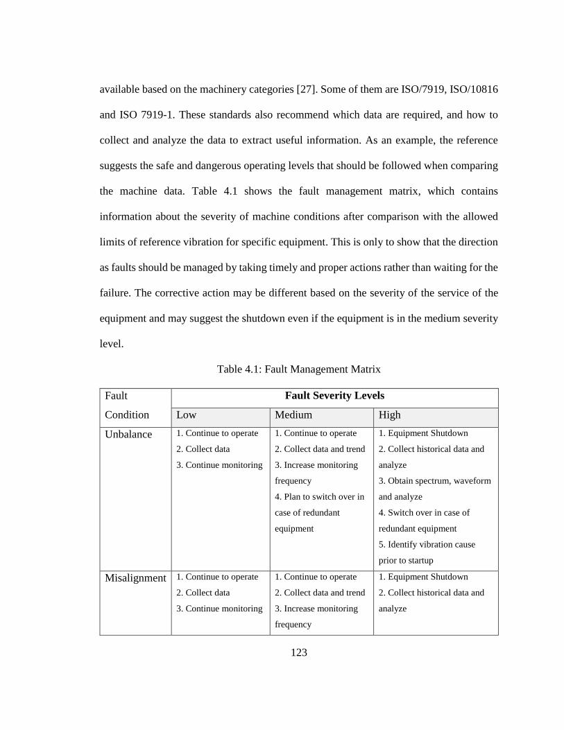
123
available based on the machinery categories [27]. Some of them are ISO/7919, ISO/10816
and ISO 7919-1. These standards also recommend which data are required, and how to
collect and analyze the data to extract useful information. As an example, the reference
suggests the safe and dangerous operating levels that should be followed when comparing
the machine data. Table 4.1 shows the fault management matrix, which contains
information about the severity of machine conditions after comparison with the allowed
limits of reference vibration for specific equipment. This is only to show that the direction
as faults should be managed by taking timely and proper actions rather than waiting for the
failure. The corrective action may be different based on the severity of the service of the
equipment and may suggest the shutdown even if the equipment is in the medium severity
level.
Table 4.1: Fault Management Matrix
Fault
Condition
Fault Severity Levels
Low Medium High
Unbalance 1. Continue to operate
2. Collect data
3. Continue monitoring
1. Continue to operate
2. Collect data and trend
3. Increase monitoring
frequency
4. Plan to switch over in
case of redundant
equipment
1. Equipment Shutdown
2. Collect historical data and
analyze
3. Obtain spectrum, waveform
and analyze
4. Switch over in case of
redundant equipment
5. Identify vibration cause
prior to startup
Misalignment 1. Continue to operate
2. Collect data
3. Continue monitoring
1. Continue to operate
2. Collect data and trend
3. Increase monitoring
frequency
1. Equipment Shutdown
2. Collect historical data and
analyze
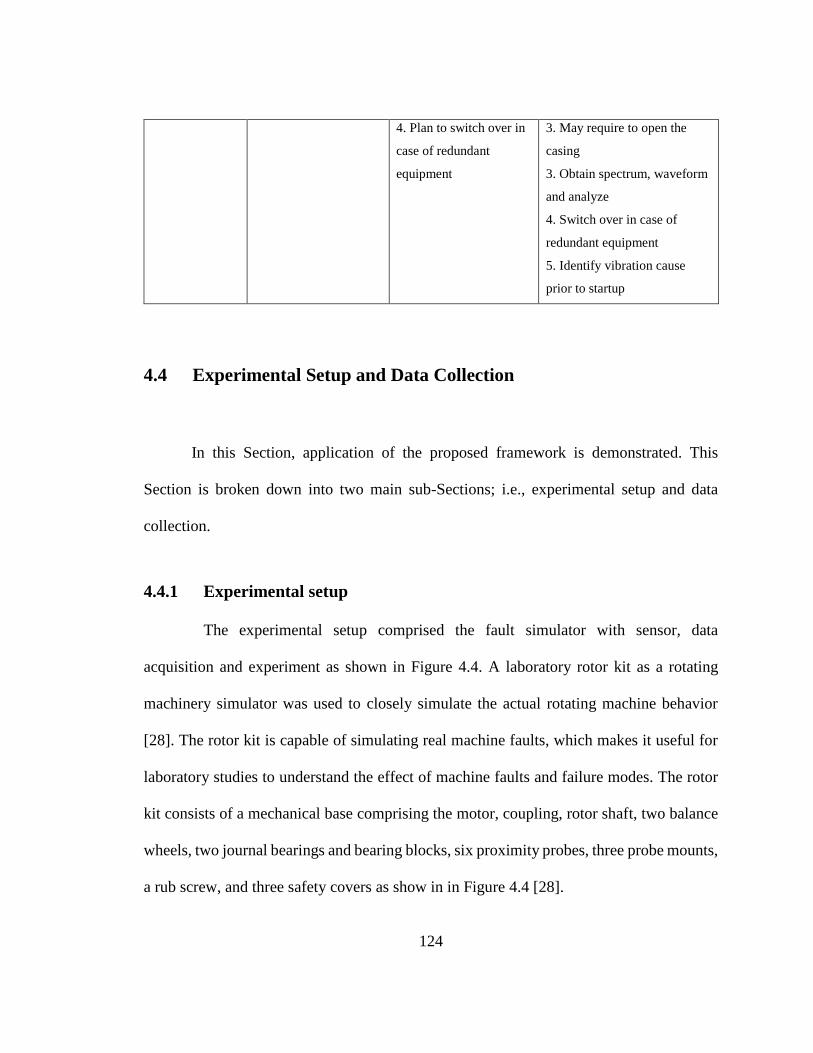
124
4. Plan to switch over in
case of redundant
equipment
3. May require to open the
casing
3. Obtain spectrum, waveform
and analyze
4. Switch over in case of
redundant equipment
5. Identify vibration cause
prior to startup
4.4 Experimental Setup and Data Collection
In this Section, application of the proposed framework is demonstrated. This
Section is broken down into two main sub-Sections; i.e., experimental setup and data
collection.
4.4.1 Experimental setup
The experimental setup comprised the fault simulator with sensor, data
acquisition and experiment as shown in Figure 4.4. A laboratory rotor kit as a rotating
machinery simulator was used to closely simulate the actual rotating machine behavior
[28]. The rotor kit is capable of simulating real machine faults, which makes it useful for
laboratory studies to understand the effect of machine faults and failure modes. The rotor
kit consists of a mechanical base comprising the motor, coupling, rotor shaft, two balance
wheels, two journal bearings and bearing blocks, six proximity probes, three probe mounts,
a rub screw, and three safety covers as show in in Figure 4.4 [28].
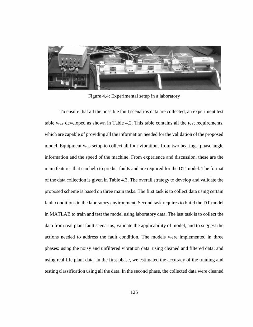
125
Figure 4.4: Experimental setup in a laboratory
To ensure that all the possible fault scenarios data are collected, an experiment test
table was developed as shown in Table 4.2. This table contains all the test requirements,
which are capable of providing all the information needed for the validation of the proposed
model. Equipment was setup to collect all four vibrations from two bearings, phase angle
information and the speed of the machine. From experience and discussion, these are the
main features that can help to predict faults and are required for the DT model. The format
of the data collection is given in Table 4.3. The overall strategy to develop and validate the
proposed scheme is based on three main tasks. The first task is to collect data using certain
fault conditions in the laboratory environment. Second task requires to build the DT model
in MATLAB to train and test the model using laboratory data. The last task is to collect the
data from real plant fault scenarios, validate the applicability of model, and to suggest the
actions needed to address the fault condition. The models were implemented in three
phases: using the noisy and unfiltered vibration data; using cleaned and filtered data; and
using real-life plant data. In the first phase, we estimated the accuracy of the training and
testing classification using all the data. In the second phase, the collected data were cleaned

126
by taking out the possible noise areas, i.e. startup data. At the end, we used real machine
data to validate the applicability of model in detecting faults in real plant conditions.
Table 4.2: Experimental Setup for the Laboratory Test
Unbalance Misalignment Labels
Test 1 0 0 0
Test 2 2.2 grams 0 1
Test 3 4.4 grams 0 2
Test 4 0 Minimum 3
Test 5 0 Maximum 4
Test 6 4.4 grams Maximum 5
Table 4.3: Data Collection Strategy for the Test
Test 1-6 Speed *DE-X *DE-Y *NDE-X *NDE-Y Phase(1X) Overall
Amplitude (1X)
Units rpm Microns microns microns microns Degrees microns
* DE is Drive End and NDE is Non Drive End
4.4.2 Vibration Data Collection
Vibration data collected as Test 1 represents the baseline, which is the "no fault"
or a baseline condition. Tests 2-6 represent different fault conditions with different
magnitudes. The conditions of the tests were set on the test rig and the data were collected
with a certain frequency to ensure the transient or spikes in the data are not missed. Two
levels of unbalance data were collected, which were 2.2 grams and 4.4 grams. Two levels

127
of combined misalignment were introduced and classified as minimum and maximum, as
it was really difficult to numerically measure and differentiate the angular and vertical
misalignments on the machinery simulator kit. Experiments were designed to ensure that
all the required data in terms of faults and features are captured for the study. Tests for
unbalance and misalignment were conducted independently, and then a worst case scenario
of the combined fault tests was run to capture common machine operating conditions. The
test plan shown in Table 4.2 ensured that all the critical conditions were considered and
tested. It would be noted that Test 6 was designed to run the combined effect of faults with
the highest severity. Labels were assigned to the different machine conditions with "0"
representing "normal condition" and 5 representing the “worst condition”.
The rotor kit was set up to ensure that it is perfectly balanced with no misalignment.
Data were collected to startup and shutdown the simulator for all the fault conditions and
a baseline test with no faults. Features that were selected in data acquisition included speed,
overall amplitude, 1X amplitude and 1X phase. These features were selected based on
engineering understanding and experience with the machines. The target variable was the
operational condition of the machine. The data initially consisted of 8,491 samples
representing different degrees of these faults. Frequency components of unbalance
conditions can be observed in waterfall plots as shown in Figure 4.5. In base condition,
there is no significant component of 1X of speed but with the introduction of unbalance,
1X of speed component becomes dominant. There are some other orders can be observed
in waterfall plot at different speeds but they are not dominant. A bode plot of an unbalance
condition of 2.2 grams is shown in Figure 4.6 to understand the effect of unbalance on
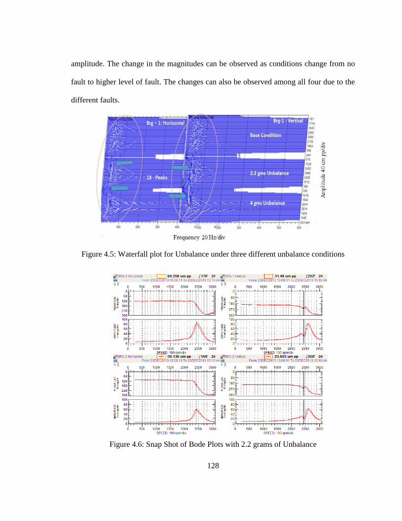
128
amplitude. The change in the magnitudes can be observed as conditions change from no
fault to higher level of fault. The changes can also be observed among all four due to the
different faults.
Figure 4.5: Waterfall plot for Unbalance under three different unbalance conditions
Figure 4.6: Snap Shot of Bode Plots with 2.2 grams of Unbalance

129
Descriptive statistics of the vibration data, used both from the rotating equipment
simulator and real plant, are given in Tables 4.4 and 4.5. The detail of the data used
provides statistics for comparative analysis. The common parameters like mean, standard
deviation and count, are presented the tables below.
Table 4.4: Equipment Simulator Descriptive Data Statistics
Speed
Overall
Amplitude Amplitude Phase
Mean 2183.8 27.0 18.4 155.9
Standard Error 8.1 0.3 0.3 1.0
Standard Deviation 647.4 22.1 22.7 83.1
Sample Variance 419163.9 486.7 513.9 6912.6
Range 2038.0 168.8 169.8 359.0
Count 6460.0 6460.0 6460.0 6460.0
Table 4.5: Real Plant Descriptive Data Statistics
Speed
Overall
Amplitude Amplitude Phase
Mean 1537.8 61.9 55.6 183.0
Standard Error 16.0 1.3 1.3 1.5
Standard Deviation 641.9 53.4 53.1 61.9
Sample Variance 412093.1 2851.5 2818.9 3831.0
Range 2324.0 165.4 164.9 270.0
Count 1619.0 1619.0 1619.0 1619.0
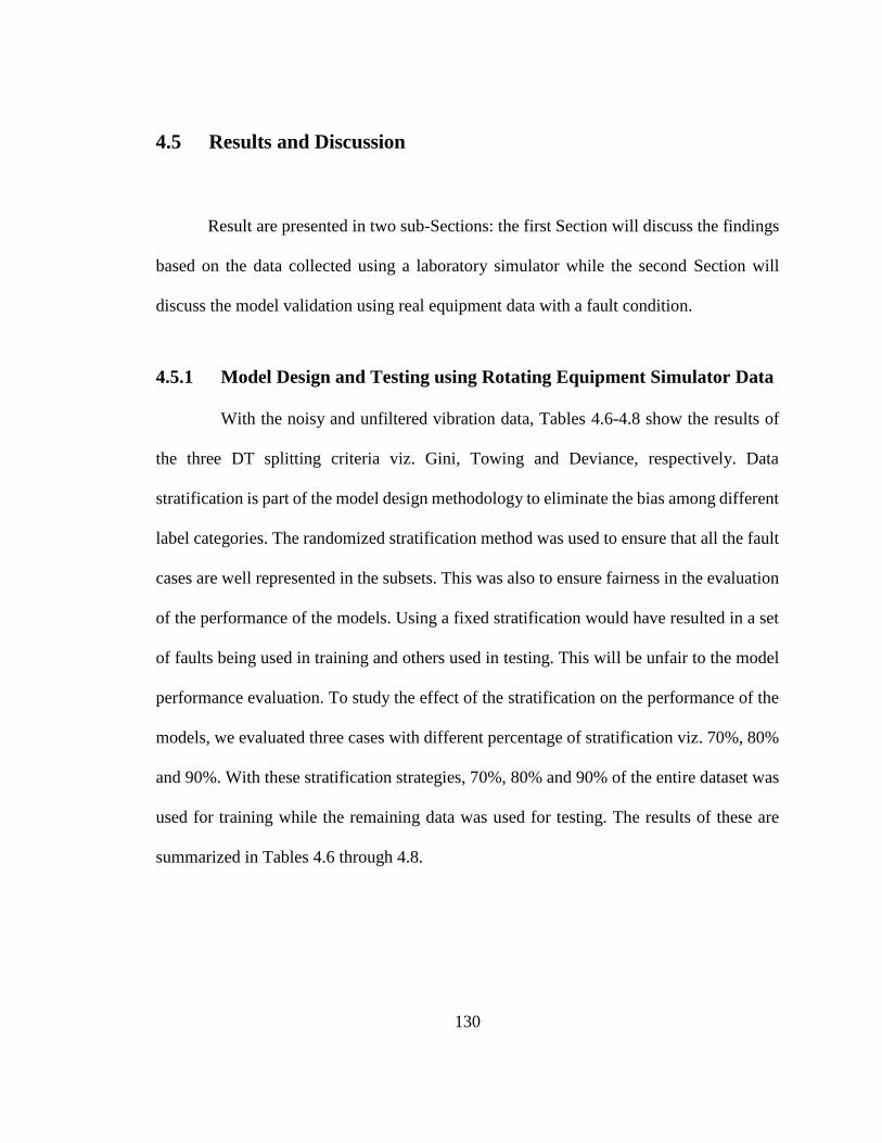
130
4.5 Results and Discussion
Result are presented in two sub-Sections: the first Section will discuss the findings
based on the data collected using a laboratory simulator while the second Section will
discuss the model validation using real equipment data with a fault condition.
4.5.1 Model Design and Testing using Rotating Equipment Simulator Data
With the noisy and unfiltered vibration data, Tables 4.6-4.8 show the results of
the three DT splitting criteria viz. Gini, Towing and Deviance, respectively. Data
stratification is part of the model design methodology to eliminate the bias among different
label categories. The randomized stratification method was used to ensure that all the fault
cases are well represented in the subsets. This was also to ensure fairness in the evaluation
of the performance of the models. Using a fixed stratification would have resulted in a set
of faults being used in training and others used in testing. This will be unfair to the model
performance evaluation. To study the effect of the stratification on the performance of the
models, we evaluated three cases with different percentage of stratification viz. 70%, 80%
and 90%. With these stratification strategies, 70%, 80% and 90% of the entire dataset was
used for training while the remaining data was used for testing. The results of these are
summarized in Tables 4.6 through 4.8.
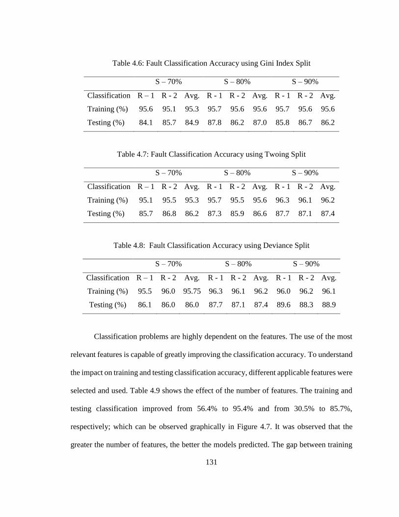
131
Table 4.6: Fault Classification Accuracy using Gini Index Split
S – 70% S – 80% S – 90%
Classification R – 1 R - 2 Avg. R - 1 R - 2 Avg. R - 1 R - 2 Avg.
Training (%) 95.6 95.1 95.3 95.7 95.6 95.6 95.7 95.6 95.6
Testing (%) 84.1 85.7 84.9 87.8 86.2 87.0 85.8 86.7 86.2
Table 4.7: Fault Classification Accuracy using Twoing Split
S – 70% S – 80% S – 90%
Classification R – 1 R - 2 Avg. R - 1 R - 2 Avg. R - 1 R - 2 Avg.
Training (%) 95.1 95.5 95.3 95.7 95.5 95.6 96.3 96.1 96.2
Testing (%) 85.7 86.8 86.2 87.3 85.9 86.6 87.7 87.1 87.4
Table 4.8: Fault Classification Accuracy using Deviance Split
S – 70% S – 80% S – 90%
Classification R – 1 R - 2 Avg. R - 1 R - 2 Avg. R - 1 R - 2 Avg.
Training (%) 95.5 96.0 95.75 96.3 96.1 96.2 96.0 96.2 96.1
Testing (%) 86.1 86.0 86.0 87.7 87.1 87.4 89.6 88.3 88.9
Classification problems are highly dependent on the features. The use of the most
relevant features is capable of greatly improving the classification accuracy. To understand
the impact on training and testing classification accuracy, different applicable features were
selected and used. Table 4.9 shows the effect of the number of features. The training and
testing classification improved from 56.4% to 95.4% and from 30.5% to 85.7%,
respectively; which can be observed graphically in Figure 4.7. It was observed that the
greater the number of features, the better the models predicted. The gap between training
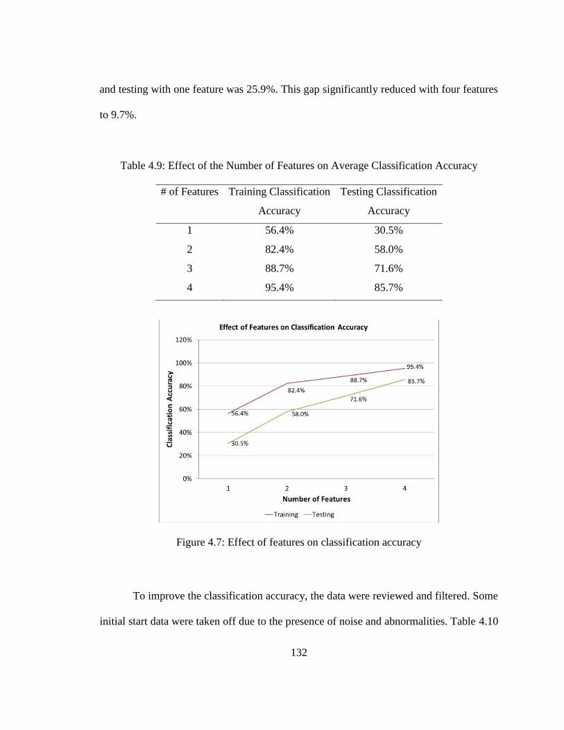
132
and testing with one feature was 25.9%. This gap significantly reduced with four features
to 9.7%.
Table 4.9: Effect of the Number of Features on Average Classification Accuracy
# of Features Training Classification
Accuracy
Testing Classification
Accuracy
1 56.4% 30.5%
2 82.4% 58.0%
3 88.7% 71.6%
4 95.4% 85.7%
Figure 4.7: Effect of features on classification accuracy
To improve the classification accuracy, the data were reviewed and filtered. Some
initial start data were taken off due to the presence of noise and abnormalities. Table 4.10

133
shows the results after data cleanup and a significant improvement was noticed. The testing
classification accuracy was improved by 5-6% and testing accuracy marginally improved
by 2%. There was no significant difference noticed among the three split criteria, but the
Deviance split performed slightly better than the other two. The stratification effect shows
slight improvement in classification as we moved from 70-90%. The combined effect of
stratification and splitting criteria can be seen in Figure 4.8. The training and testing graphs
correspond to the three training options that are available in the Decision Tree algorithm,
Gini, Twoing and Deviance at 70, 80 and 90% stratification respectively. Each of these
algorithms has been described in Section 4.3. Gini is the commonly used algorithm,
however, we found it necessary to investigate the effect of the other algorithms. Deviance
algorithm performed slight better than the other two algorithms in this case. On the average,
the slight positive change is not shown only in the 90% stratification but also in the 80%.
The reason for improvement, which also confirms our conclusion, is that generalization
(testing) improves with increase in the number of training samples, when the proportion of
the training stratification increases.
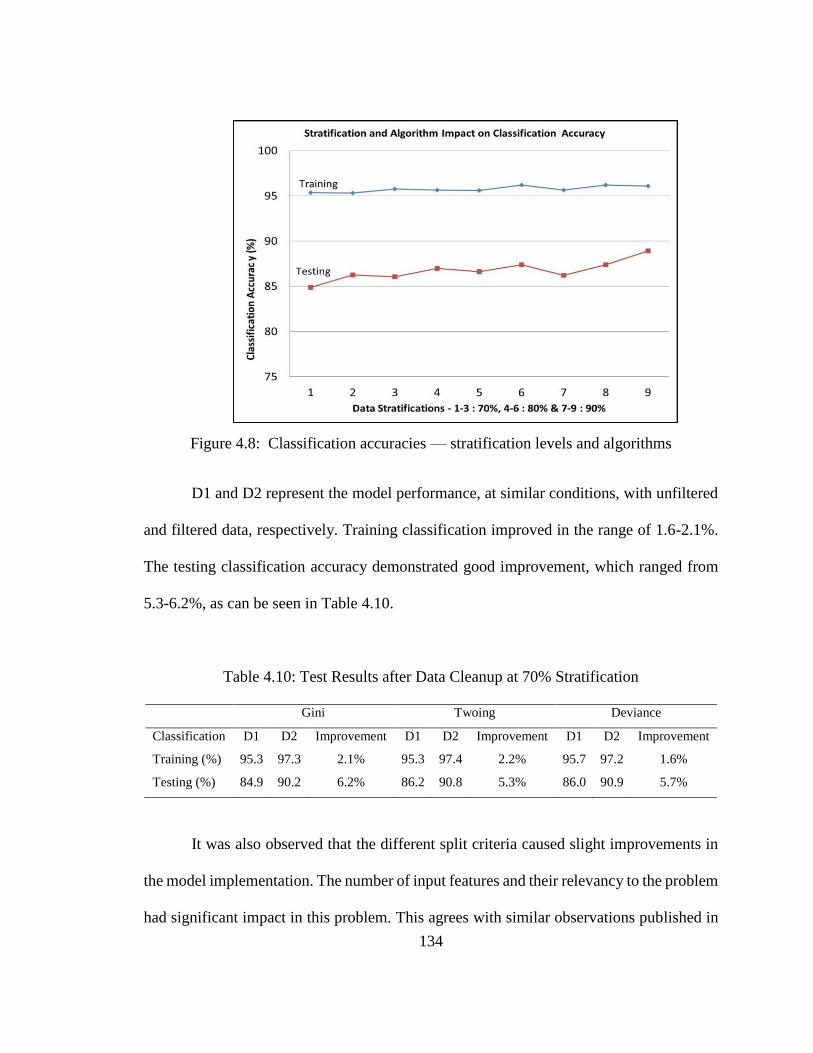
134
Figure 4.8: Classification accuracies — stratification levels and algorithms
D1 and D2 represent the model performance, at similar conditions, with unfiltered
and filtered data, respectively. Training classification improved in the range of 1.6-2.1%.
The testing classification accuracy demonstrated good improvement, which ranged from
5.3-6.2%, as can be seen in Table 4.10.
Table 4.10: Test Results after Data Cleanup at 70% Stratification
Gini Twoing Deviance
Classification D1 D2 Improvement D1 D2 Improvement D1 D2 Improvement
Training (%) 95.3 97.3 2.1% 95.3 97.4 2.2% 95.7 97.2 1.6%
Testing (%) 84.9 90.2 6.2% 86.2 90.8 5.3% 86.0 90.9 5.7%
It was also observed that the different split criteria caused slight improvements in
the model implementation. The number of input features and their relevancy to the problem
had significant impact in this problem. This agrees with similar observations published in
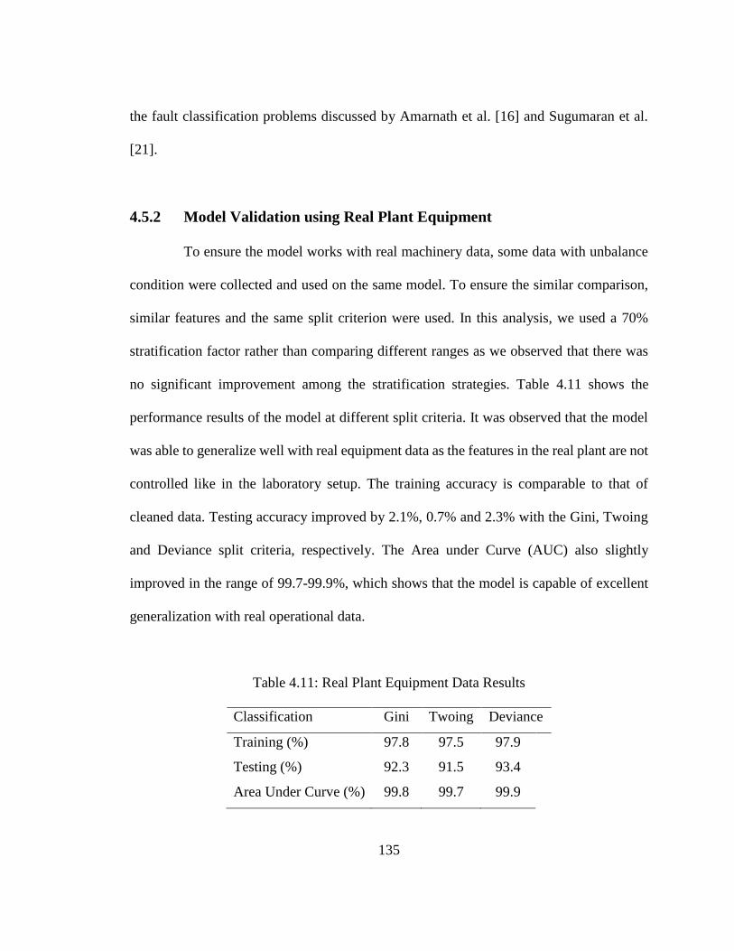
135
the fault classification problems discussed by Amarnath et al. [16] and Sugumaran et al.
[21].
4.5.2 Model Validation using Real Plant Equipment
To ensure the model works with real machinery data, some data with unbalance
condition were collected and used on the same model. To ensure the similar comparison,
similar features and the same split criterion were used. In this analysis, we used a 70%
stratification factor rather than comparing different ranges as we observed that there was
no significant improvement among the stratification strategies. Table 4.11 shows the
performance results of the model at different split criteria. It was observed that the model
was able to generalize well with real equipment data as the features in the real plant are not
controlled like in the laboratory setup. The training accuracy is comparable to that of
cleaned data. Testing accuracy improved by 2.1%, 0.7% and 2.3% with the Gini, Twoing
and Deviance split criteria, respectively. The Area under Curve (AUC) also slightly
improved in the range of 99.7-99.9%, which shows that the model is capable of excellent
generalization with real operational data.
Table 4.11: Real Plant Equipment Data Results
Classification Gini Twoing Deviance
Training (%) 97.8 97.5 97.9
Testing (%) 92.3 91.5 93.4
Area Under Curve (%) 99.8 99.7 99.9

136
Comparison of classification accuracy was performed to show the difference
between real plant data and laboratory data as shown in Figure 4.9. The plant data showed
an average of 6.7% training classification improvement and around 2.3% for testing. The
improvement shown in the plant data is extremely beneficial due the potential improvement
by applying proposed model to real life industrial problems.
Figure 4.9: Classification accuracy comparison
The results of the fault detection accuracy using real plant data are shown in Table
4.12. Real plant machinery vibration data were used to detect unbalance fault using the DT
based proposed algorithm. The model has shown that on average the model has the
capability of detecting faults correctly in ranges from 98.4 - 99.4% with an incorrectly
detecting a fault range from 0.53 - 1.26%. In published research [16], a DT based fault
detection model was proposed using acoustic signals for fault detection. The results showed
the true positive accuracy ranges from 93.3 - 96.7% and incorrect detection was around 3.3

137
- 6.7%. In another work presented by Sugumaran et al [21], where the vibration signals are
used to detect faults, 86% of true accuracy and 14% of incorrect detection is reported. We
acknowledge that there are some differences among other published works [16-17, 20, 22]
and this work, such as different systems, different faults and sensors. However, the
commonality is that all have used DTs based models for fault detection. Based on this
commonality, the proposed model in this research delivers a true positive level that is
comparable to the results reported by others utilizing similar methods.
Table 4.12: Fault detection using the proposed DT based model
Description Fault Labeled
Correctly (%)
Fault Labeled
Incorrectly (%)
Average – Gini 99.47 0.53
Average – Twoing 98.44 1.56
Average – Deviance 98.74 1.26
4.6 Conclusion
Fault detection and management plays a vital role in managing system availability.
An application of DTs for detecting machinery faults and addressing them through proper
management action has been successfully presented. A DTs based predictive model was
developed to detect faults and their severity using vibration data. The overall testing
classification accuracy was about 97% and the testing accuracy was 92% has achieved,
which is comparable with other DTs based fault detection models.
138
We observed a 5% overall improvement in the classification accuracies when
filtered data were used instead of an initial noisy and unfiltered data. Results also showed
significant improvements using optimal features as the training classification accuracy with
4 features is around 95% and testing classification accuracy is around 85%. The highest
classification accuracy performance of 85% with 7 features and about 83% with 4 features
is also reported in another work [21], which is in-line with this work finding. The model
validation using real plant data compared to laboratory data was outstanding as the testing
and training accuracies improved by 6.7% and 2.3%, respectively. The proposed model has
shown that on average the model has the capability of detecting faults correctly in ranges
from 98.4 - 99.4% with an incorrectly detecting fault range between 0.5 - 1.2%. This indeed
is a great benefit for plant engineering in handling faults.
Although, this work is limited to three fault conditions, but model can be extended
to dynamic online system to diagnose other machinery faults under different operating
conditions. The other limitation experienced during the development of this model is
changing operating conditions and possible fault scenarios in testing data. To address this
limitation, we have developed the dynamic model which has capability of updating the
training sets to include the new possible scenarios without building the model from scratch.
The performance of the proposed model demonstrated that it can be practically used for
detecting fault conditions and their severities in real and operational scenarios of rotating
machines. Along with detection of faults, the proposed fault management strategy also
plays an important role in enhancing plant availability. The machine learning-based holistic

139
approach from detection to management proposed would be of great help to avoid
unscheduled breakdowns and improving the availability of facilities.

140
CHAPTER 5
A MULTI-CONSTRAINED MAINTENANCE SCHEDULING
OPTIMIZATION 5
Abstract
A maintenance scheduling optimization model considering equipment risk, total
maintenance cost, system reliability, and availability is proposed. This work is motivated
by gas processing operator concern for high maintenance costs, poor availability and
reliability caused by inefficient maintenance scheduling. The approach presented in this
5 This Chapter is based on the published work in a peer-reviewed journal. Qadeer Ahmed, Kamran
S. Moghaddam, Syed A. Raza, Faisal I. Khan (2015), “A Multi Constrained Maintenance
Scheduling Optimization Model for Hydrocarbon Processing Facilities,” Journal of Risk and
Reliability Engineering, accepted for publication. To minimize the duplication, all the references
are listed in the reference list. The contribution of the authors is presented in Section titled, “Co-
authorship Statement”. The contribution of the authors is presented in Section titled, “Co-
authorship Statement”.

141
Chapter addresses the optimization of maintenance costs by efficiently scheduling
maintenance tasks subject to reliability and availability constraints. Four maintenance
actions are considered for equipment; namely corrective, replacement, maintenance, and
inspection. The proposed solution develops maintenance schedules for complex repairable
system with equipment operating in series. Two single objective, nonlinear mathematical
models are presented to find the optimal maintenance cost subject to reliability and system
reliability subject to availability constraint. A goal programming model is also proposed to
simultaneously deal with multiple criteria based on their importance and defined goals. A
gas absorption system of a hydrocarbon processing facility is used to ensure the practicality
of the proposed formulation to real industry problems. A comparison of existing and
proposed formulation is carried out to show that the proposed optimization approach is an
efficient method for optimizing maintenance schedules and flexibility to adjust schedules
in complex operating systems.
5.1 Introduction
Equipment availability and effective maintenance are two strongly related
important criteria for ensuring safe operative system that is capable of handling production
requirements. Proper maintenance of deteriorating equipment prevents unwanted
breakdowns, which lead to poor system reliability and high production cost. Low system
reliability and availability negatively impact the company’s image and commitment to
deliver on-time quality products. Equipment breakdowns are unsafe and generally cost the

142
company a huge amount of capital along with jeopardizing its reputation in industry. These
issues encourage organizations to develop smarter and effective strategies to significantly
improve maintenance schedules to achieve safe operations with high equipment
availability and lower costs. A balance between expense and profit is also an objective for
any organization to stay in business and meet the expectations of stakeholders. The benefits
of maintenance schedule optimization have led researchers to develop optimization
methods and techniques, which have been proposed and published over the years. The
proposed methods have a wide range of objectives, constraints, and optimization
methodologies with a common goal of achieving low cost and effective solutions. In
general, maintenance is critical to ensure system availability, but advances in technology
and new heuristic algorithms have paved new roads to efficiently optimize maintenance
actions. Maintenance has become a vital function as maintenance cost is a significant
portion of the total operating cost in asset intensive industries such as petrochemical and
gas plants. Different types of maintenance tasks have been introduced and practiced in
industry including preventive, predictive, reactive, and corrective maintenance. Realistic
maintenance requirements must be properly understood and action plans should be
properly developed to address the equipment failure modes. Maintenance has two critical
aspects; what and when? “What” relates to a maintenance task or activity; and “when”
explains the time characteristics of maintenance. Both features are critical and, if not
handled correctly, can negatively impact both availability and cost. We will concentrate on
maintenance scheduling optimization, which includes corrective, preventive, replacement,
and inspection maintenance.
143
Maintenance is defined as “a task performed to retain or restore a function of
equipment during its life cycle” [1]. Much maintenance, including preventive, corrective,
reactive, operational, and others are available to ensure improved functionality of the
equipment. In this research, we have considered four major maintenance tasks, namely
inspection, maintenance, corrective, and replacement. Preventive maintenance can be
defined as, “a fundamental, planned maintenance activity designed to improve equipment
life and avoid any unplanned maintenance activity [1].” Preventive maintenance has a
direct impact on availability necessitating selection of appropriate tasks at proper intervals.
Corrective maintenance is defined as “a maintenance task performed to repair or restore
function of equipment after a breakdown.” This category of maintenance is often expensive
due to the failure of multiple components in an unscheduled breakdown event [2].
Replacement maintenance is a task where the component of equipment is replaced based
on the established life of components. In this maintenance activity, the cost is lower due to
the prior planning of component replacement. An inspection task is defined as “the task
performed on equipment while in operation to spot any abnormality.” This task generally
requires cleaning, lubrication, minor adjustment, and reporting of any abnormality found
during inspection. While inspection is generally performed by plant operators; other
maintenance tasks are performed by maintenance technicians and maintenance engineers.
Predictive maintenance is also a maintenance activity classified as “a technique that helps
determine the condition of in-service equipment in order to predict when maintenance
should be performed” [3]. A predictive approach offers some benefits over other
maintenance actions, but requires good quality data and experienced individuals to

144
interpret the data to make correct decisions. There is a great effort in development of smart
diagnostics and prognostics algorithms to enhance the prediction accuracy; but it is not part
of this work.
Maintenance optimization is a very important area of research due to its potential
benefits to industry. It has gained exposure as a result of significant change in traditional
and contemporary maintenance, where maintenance has no longer only an organization’s
support function but considered as business driver. These days maintenance focus is not
only to keep the plant in operation but emphasis is also on efficient utilization of equipment.
Maintenance management becomes extremely important in industries such as liquefied
natural gas (LNG) due to the presence of a large number and wide variety of critical
equipment. Processing LNG is a hazardous process requiring considerable safety. It is a
cryogenic process where the operating temperature is around -164°C and any failure can
have catastrophic consequences. As a result, effective and optimized maintenance is a key
to safety, optimal availability, and reduced overall maintenance cost of the facilities.
Maintenance in hydrocarbon processing facilities is important not only because of critical
application but also unplanned breakdown equipment cost is significant in terms of
production loss and customer satisfaction by missing the promised deliveries. These are
some reasons that many researchers from industry and academia are involved in the
formulation of new maintenance optimization models and algorithms to address this area.
Maintenance optimization has progressed through different stages as the knowledge and
tools become available to solve complex problems. Advances in optimization algorithms
have paved the road for solving multi-objective maintenance optimization. Earlier,

145
maintenance optimization models were more focused on cost minimization and
maintenance task schedules. This may be due to the limitation of the advanced data
processing tools, i.e., computerized maintenance management systems (CMMS), asset
performance management (APM) systems, efficient simulators and high speed processors,
along with lack of understanding of the influence of maintenance relationships with other
variables. Developments in technology and innovation have introduced processing of
utilized data and data mining to understand equipment failure modes and their
consequences for developing the right maintenance actions. Understanding risk and
consequences of failure of equipment greatly helps in the selection of optimal execution of
maintenance intervals through risk-based prioritization. Risk-based maintenance
scheduling optimization can greatly influence maintenance costs as it addresses equipment
criticality and prioritization of tasks accordingly. Risk is a product of probability of
equipment failure and its consequence to environment, production and personnel [4]. The
term, Equipment Risk Index (ERI) classifies the equipment criticality and helps to
prioritize maintenance actions. This risk index ranges from high to low; a higher ERI score
is used to determine the maintenance priority.
Nowadays, extensive research in maintenance scheduling optimization is being
conducted due to its usefulness and benefits to industry. This includes maintenance
scheduling using dynamic programming and introduction of heuristic algorithms in
maintenance optimization with reliability, availability, and budget criteria [5]. In other
work, integer programming and branch-and-bound was introduced. Branch-and-bound is a
technique for solving integer linear programming (ILP) problems but integer programming

146
has limitations in solving nonlinear objective functions [6]. Some other meta-heuristics,
like genetic algorithms, have been introduced to effectively handle optimization problems
in maintenance and reliability contexts [7-9]. A genetic algorithm (GA) is efficient in
addressing nonlinearity. Most meta-heuristic algorithms are approximate and mostly non-
deterministic; similarly, GAs are approximate and cannot guarantee an optimal solution.
Newer research covers many areas in maintenance optimization, which includes cost,
manpower, resources, operation, and equipment shutdown schedules to reap real benefit
by properly optimizing maintenance tasks. In this work, different maintenance tasks are
used to minimize maintenance cost subject to reliability, and maximize reliability subject
to system availability. A gas absorption unit in a gas processing plant is used to implement
the proposed maintenance schedule optimization.
5.1.1 Description of a Natural Gas Treatment and Gas Absorption System
A natural gas processing plant is asset intensive and demands proper care of
equipment to ensure safe and continuous operation. In these asset intensive plants, proper
and timely maintenance is vital to guarantee safety and meet customers’ demands from
around the globe by producing product on schedule. This makes maintenance scheduling
and optimization an important function in process plants. Gas is produced at plants in both
forms, i.e., gas and liquid. In liquid form, the temperature of natural gas is usually around
-160°C and the volume is around 1/600 times that of gas at room temperature. A general
gas process consists of following several major steps as shown in Figure 5.1. Raw gas is
received from a reservoir to the inlet receiving area, which is followed by treatment of
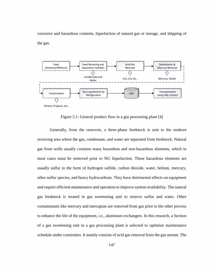
147
corrosive and hazardous contents, liquefaction of natural gas or storage, and shipping of
the gas.
Figure 5.1: General product flow in a gas processing plant [4]
Generally, from the reservoir, a three-phase feedstock is sent to the onshore
receiving area where the gas, condensate, and water are separated from feedstock. Natural
gas from wells usually contains many hazardous and non-hazardous elements, which in
most cases must be removed prior to NG liquefaction. These hazardous elements are
usually sulfur in the form of hydrogen sulfide, carbon dioxide, water, helium, mercury,
other sulfur species, and heavy hydrocarbons. They have detrimental effects on equipment
and require efficient maintenance and operation to improve system availability. The natural
gas feedstock is treated in gas sweetening unit to remove sulfur and water. Other
contaminants like mercury and mercaptan are removed from gas prior to the other process
to enhance the life of the equipment, i.e., aluminum exchangers. In this research, a Section
of a gas sweetening unit in a gas processing plant is selected to optimize maintenance
schedule under constraints. It mainly consists of acid gas removal from the gas stream. The
Feed
(Onshore/Offshore)Feed Receiving and Separation Facilities
Acid Gas Removal
Dehydration & Mercury Removal
FractionationGas Liquefaction by
RefrigerationLNG
Transportationusing LNG Carriers
Condensate and Water
H2S, CO2 etc.. Mercury, Water
Ethane, Propane, etc..

148
absorption unit is very critical for both safety and production as it absorbs hydrogen sulfide
and carbon dioxide. These gases are highly corrosive and will cause severe damage to
cryogenic vessels during the liquefaction process; therefore, it is necessary to remove these
gases and contaminants before they reach the final stages of liquefaction. In the acid gas
absorbers, hydrogen sulfide and carbon dioxide gases are absorbed completely in the
solvent and sweet natural gas is routed to the gas drying Section and liquefaction units.
Since the natural gas sweetening process is very critical in terms of operations and
commitment needed for production, the availability and reliability of all the equipment
remains under focus and operational integrity is monitored closely. For reliable processing
of the gas sweetening unit, all required equipment must be maintained for overall operation
of the plant.
5.1.2 Research Objective and Contributions
While maintenance is one of the important activities in processing facilities; it
should not be taken as an inevitable source of cost savings to ensure continuous and safe
operation. The importance of maintenance management and optimization is reflected in
many publications by researchers, as discussed in Section 5.2 of this Chapter. We have
addressed optimal maintenance scheduling in a gas absorption system of a natural gas
processing plant where maintenance is critical and extremely important due to the risk
posed by high gas pressure, low operating temperatures, and the presence of hazardous
hydrocarbons. We expanded previous work by developing a framework and mathematical
formulation that is applicable to repairable systems using four different maintenance

149
actions of inspection, preventive, corrective, and replacement [5]. Corrective maintenance
action due to equipment breakdown is also considered, which can negatively impact
availability, reliability, and safe work environment. The advantages offered by optimal
maintenance scheduling are two-fold; it minimizes maintenance durations to ensure plant
availability and directs optimum maintenance scheduling actions to keep the maintenance
cost low for a desired level of availability and reliability. This work mainly presents four
major contributions, which are:
1. Developed two single objective optimization models, (1) minimization of
maintenance cost subject to reliability constraints, and (2) maximization of system
reliability subject to availability constraints.
2. Developed a goal programming model that simultaneously considers multiple
criteria; cost, reliability, and availability. This model was applied on a gas
absorption system using different goals and weights to obtain Pareto-optimal
maintenance schedules to demonstrate the formulation applicability to real industry
problems.
3. Maintenance costs, maintenance duration, system reliability, and availability of an
existing gas absorption system were estimated to compare with proposed
formulation results.
4. Introduced the concept of the ERI while handling real plant maintenance
prioritization. The ERI is used to classify equipment criticality, which helps with
prioritizing the maintenance task particularly during a resource or schedule

150
constraint. The effect of the ERI on maintenance schedules is presented in Section
5.3.2.
This work proposes a maintenance scheduling optimization approach that
minimizes maintenance costs subject to desired plant reliability and availability targets.
Section 5.1 provides the introduction of maintenance, maintenance optimization, and a
brief description of a gas absorption system; and Section 5.2 provides the literature survey.
Section 5.3 encompasses the problem formulation and constraint development. In Section
5.4, three optimization models are developed. In Section 5.5, an analysis of the proposed
models is carried out. Section 5.6 presents the results of developed model when applied to
a gas absorption system and maintenance cost comparison is performed using the existing
maintenance practices. Finally, in Section 5.7 the results are summarized in a conclusion.
5.2 Literature Research
Maintenance and reliability optimization have been investigated by many
researchers for the last couple of decades. In general, optimization is a mathematical model
to find the best or optimal solution from all possible solutions. These models have been
developed to optimize different objective functions, including but not limited to, revenues,
maintenance schedules, system availability, and costs in different industries. In this work,
we are focused on maintenance scheduling optimization of a processing facility, and so
some related work is explored. Several optimization techniques in single objective

151
optimization have been introduced, and now researchers are more focused on multi-
objective optimization due to its extensive application and utilization in real life
applications. A single-objective optimization problem in which more than one criterion is
considered simultaneously becomes multi-objective optimization [10]. Maintenance is
important to ensure availability and manage maintenance cost, which makes it an
interesting area of research both from an academia and industry perspective.
In this Section, we have discussed the work performed in the area of maintenance
schedule optimization. Maintenance optimization in hydrocarbon facilities is not explored
extensively, which provides an opportunity to expand in this area. A joint production and
maintenance scheduling model with multiple preventive maintenance services is presented
[11]. To handle this problem, a mixed integer nonlinear programming model is developed
and then a population-based variable neighborhood search algorithm is devised for a
solution method. The simulation outcome shows the outstanding performance of traditional
genetic algorithms and basic variable neighborhood search in terms of both effectiveness
and robustness. A cost minimization objective function with system reliability is presented
to optimize the maintenance schedule [12]. A component-based heuristic algorithm was
developed to solve the optimization model for a real field system while maintaining the
architecture or components in a traction catenary system. A meta-heuristic model is
presented for maintenance scheduling of generators using hybrid improved binary particle
swarm optimization based coordinated deterministic and stochastic approach [13]. The
objective function focuses on reducing the loss of load probability and minimizing the
annual supply reserve ratio deviation for a power system as a measure of power system

152
reliability. The proposed method yields better results by improving search performance and
better convergence characteristics compared to the other optimization methods and
conventional method. A technique based on one of the artificial immune system techniques
known as the clonal selection algorithm to obtain the optimal maintenance schedule outage
of generating units is proposed [14]. It has successfully been used to solve the maintenance
scheduling sub-problem to obtain the optimal maintenance outage of each unit.
Risk is a critical component in decision making processes and plays a vital role in
maintenance optimization. Risk-based optimizations are also gaining momentum to
explore the detrimental effects of equipment breakdowns on the operation of processing
facilities. These effects cover production revenue loss, downtime, environmental, and
safety concerns due to the unavailability of equipment. Many researchers have worked on
risk-based approaches to maintenance optimizations [15-17]. A risk-based optimization
model for system maintenance scheduling problems is proposed, which consists of
optimizing availability and the cost of the system by balancing between system
maintenance risk and failure risk [18]. A genetic algorithm is used to obtain the sequence
of maintenance actions providing a desired level of reliability with minimum system risk.
Results obtained from the modeling approach support the validity of the model in
optimizing maintenance schedules. A new version of the simulated annealing method for
solving the generator maintenance scheduling problem is presented [19]. The model
considered in this paper is formulated as a mixed integer program, with a reliability
optimality criterion, subject to a number of constraints. The proposed simulated annealing
algorithm performs very well compared to other methods on the benchmark test system
153
presented in literature. A preventive maintenance scheduling problem with interval costs
to schedule preventive maintenance of the components is proposed [20]. A study is
performed from a polyhedral and exact solution point of view, as opposed to previously
studied heuristics. As a result, the proposed model can be effectively used as a building
block to model several types of maintenance planning problems possessing deterioration
costs. A hybrid evolutionary algorithm is explored to tackle the reliability based generator
maintenance scheduling problem [21]. Uncertainties in the generating units and the load
variations are included so that a more realistic scheduling is obtained. A new local search
method, which is derived from external optimization and genetic algorithm, is presented to
tackle the problem. This method can be used as a local optimizer to further improve the
potential solutions in the genetic algorithm. An advanced progressive real coded genetic
algorithm is applied to optimize the availability of standby systems with preventive
maintenance scheduling [22]. Results from an emergency system are compared with those
obtained by some standard maintenance policies, and previously published papers.
A modified genetic algorithm approach to long-term generation maintenance
scheduling to enhance the reliability of the units is presented [23]. Maintenance scheduling
establishes the outage time scheduling of units in a particular time horizon. The proposed
methodology is used for finding the optimum preventive maintenance scheduling of
generating units in power system. The objective function is to maintain the utility power
system units as early as possible under constrains such as spinning reserve, duration of
maintenance and maintenance crew are being taken into account. A selection of multiple
maintenance strategy in process equipment is presented [24]. Three maintenance strategies

154
namely, repair maintenance, preventive maintenance, and preventive replacement on
equipment reliability was analyzed. The harmony search algorithm was designed to solve
the model, and the diversity of solutions was ensured by generating the new solution and
the replacement process. A non-dominated sorting genetic algorithm based optimization
approach is presented for an optimum maintenance to improve the average reliability of
ship's operations at sea at minimum cost [25]. The advantages are explored that can accrue
from introducing short maintenance periods for a select group of machinery, within the
constraints of mandatory operational time, over the method of following a common
maintenance interval for all the machinery. An integrated model for the joint determination
of both optimal inspection strategy and optimal repair policy is discussed for a
manufacturing system whose resulting output is subject to system state [26]. In this paper,
an intensity control model adapted to partial information provides an optimal inspection
intensity and repair degree of the system as an optimal control process to yield maximum
revenue. A numerical example is provided to illustrate the behavior of the optimal control
process. An inspection and replacement policy for a protection system is described in
which the inspection process is subject to error, and false positives and false negatives are
possible [27]. Two models are developed, one in which a false positive implies renewal of
the protection system and the other does not implies renewal. The model allows situations
in which maintenance quality differs between alternative maintainers to be investigated.
Reliability is one of the most efficient and important method to study safe operation
probability of hydraulic systems. The reliability of a hydraulic system of four rotary drilling
machines has been analyzed [28]. The data analysis shows that the time between failures
155
of two machines obey the Weibull distribution. Also, the time between failures of two other
machines obey the lognormal distribution. Later, preventive reliability-based maintenance
time intervals for 80% reliability levels for machines are presented.
The problem of determining operations and maintenance schedules for a
containership equipped with various subsystems is studied during its sailing according to
a predetermined navigation schedule [29]. A mixed integer programming model is
developed. Then, due to the complexity of the problem, a heuristic algorithm that
minimizes the sum of earliness and tardiness between the due date and the actual start time
for each maintenance activity is discussed and improvement is reported over the experience
based conventional method. A novel cost-reliability model, which allows the use of a
flexible interval between maintenance interventions, is proposed [30]. It allows a
continuous fitting of the schedules to deal with the changing failure rates of the
components. A single objective optimization model was explored to determine the optimal
maintenance policy by minimizing cost and respecting availability constraint for a series-
parallel system [31]. In [32], an overview and tutorial about multi-objective formulation is
explored. Another work proposed a multi-objective maintenance problem in relation to a
system that needs to operate without interruption between two consecutive stops with a
reliability level not lower than a fixed value. [33]. A multi-objective formulation is
proposed to minimize the cost and maximize the availability of a global system [34]. In
this proposed model, availability allocation to a repairable system at the design level is
considered rather than availability in the operating phase.

156
The complex landscape of maintenance optimization and its huge impact on
industry has received considerable attention among academia and industry to come up with
methods to develop efficient maintenance schedules. In this work, we have explored the
concept of equipment failure risk in maintenance by identifying critical equipment using
risk assessment. Goal programming is an extension of linear programming, which provides
flexibility to handle a decision concerning multiple and conflicting goals [35]. This
approach is extensively applied in optimization research. Due to its handling of multiple
criteria simultaneously, we have used goal programming to solve a model to study the
impact of cost, reliability, and availability based on defined goals and weights. Under
different goals and weights, a developed model was applied to a gas absorption system to
obtain optimized maintenance schedules. To the author’s knowledge, maintenance
scheduling optimization has a great research potential because of the complexity of
equipment failure patterns, resource availability, risk to production and society, etc. All
these constraints, i.e., maintenance factor, reliability, and availability have the potential to
explore and provide a great value to industry by developing maintenance strategies and
optimizing them. As a result, this work is expected to contribute by developing a practical
solution to the industry’s concern for efficient maintenance scheduling.
5.3 Formulation of a Maintenance Optimization Model
Effective maintenance is one of the key functional areas in industry to address plant
uptime, maintenance cost, safety, and availability. To address these objectives,
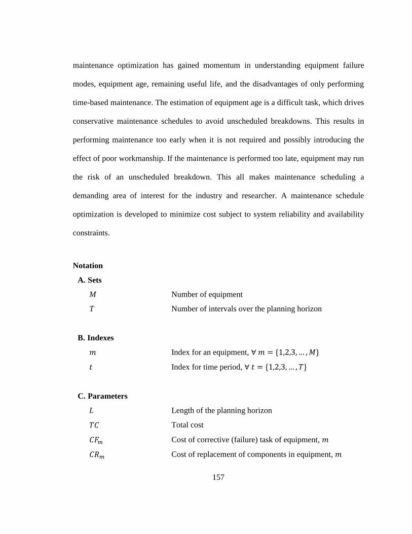
157
maintenance optimization has gained momentum in understanding equipment failure
modes, equipment age, remaining useful life, and the disadvantages of only performing
time-based maintenance. The estimation of equipment age is a difficult task, which drives
conservative maintenance schedules to avoid unscheduled breakdowns. This results in
performing maintenance too early when it is not required and possibly introducing the
effect of poor workmanship. If the maintenance is performed too late, equipment may run
the risk of an unscheduled breakdown. This all makes maintenance scheduling a
demanding area of interest for the industry and researcher. A maintenance schedule
optimization is developed to minimize cost subject to system reliability and availability
constraints.
Notation
A. Sets
M Number of equipment
T Number of intervals over the planning horizon
B. Indexes
𝑚 Index for an equipment, ∀ 𝑚 = {1,2,3, … , 𝑀}
𝑡 Index for time period, ∀ 𝑡 = {1,2,3, … , 𝑇}
C. Parameters
L Length of the planning horizon
𝑇𝐶 Total cost
𝐶𝐹𝑚 Cost of corrective (failure) task of equipment, 𝑚
𝐶𝑅𝑚 Cost of replacement of components in equipment, 𝑚
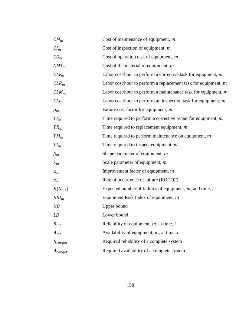
158
𝐶𝑀𝑚 Cost of maintenance of equipment, 𝑚
𝐶𝐼𝑚 Cost of inspection of equipment, 𝑚
𝐶𝑂𝑚 Cost of operation task of equipment, 𝑚
𝐶𝑀𝑇𝑚 Cost of the material of equipment, 𝑚
𝐶𝐿𝐹𝑚 Labor cost/hour to perform a corrective task for equipment, 𝑚
𝐶𝐿𝑅𝑚 Labor cost/hour to perform a replacement task for equipment, 𝑚
𝐶𝐿𝑀𝑚 Labor cost/hour to perform a maintenance task for equipment, 𝑚
𝐶𝐿𝐼𝑚 Labor cost/hour to perform an inspection task for equipment, 𝑚
𝜌𝑚 Failure cost factor for equipment, 𝑚
𝑇𝐹𝑚 Time required to perform a corrective repair for equipment, 𝑚
𝑇𝑅𝑚 Time required to replacement equipment, 𝑚
𝑇𝑀𝑚 Time required to perform maintenance on equipment, 𝑚
𝑇𝐼𝑚 Time required to inspect equipment, 𝑚
𝛽𝑚 Shape parameter of equipment, 𝑚
𝜆𝑚 Scale parameter of equipment, 𝑚
𝛼𝑚 Improvement factor of equipment, 𝑚
𝜈𝑚 Rate of occurrence of failure (ROCOF)
𝐸[𝑁𝑚𝑡] Expected number of failures of equipment, 𝑚, and time, 𝑡
𝐸𝑅𝐼𝑚 Equipment Risk Index of equipment, 𝑚
𝑈𝐵 Upper bound
𝐿𝐵 Lower bound
𝑅𝑚𝑡 Reliability of equipment, 𝑚, at time, 𝑡
𝐴𝑚𝑡 Availability of equipment, 𝑚, at time, 𝑡
𝑅𝑡𝑎𝑟𝑔𝑒𝑡 Required reliability of a complete system
𝐴𝑡𝑎𝑟𝑔𝑒𝑡 Required availability of a complete system

159
D. Decision variables
𝐴𝑆𝑚𝑡 Age of equipment, 𝑚, at the start of period, 𝑡
𝐴𝐸𝑚𝑡 Age of equipment, 𝑚, at the end of period, 𝑡
𝑋𝑚𝑡 {1 𝑀𝑎𝑖𝑛𝑡𝑒𝑛𝑎𝑛𝑐𝑒 𝑡𝑎𝑠𝑘 𝑖𝑠 𝑝𝑒𝑟𝑓𝑜𝑟𝑚𝑒𝑑 𝑓𝑜𝑟 𝑒𝑞𝑢𝑖𝑝𝑚𝑒𝑛𝑡, 𝑚, 𝑎𝑡 𝑝𝑒𝑟𝑖𝑜𝑑, 𝑡0 𝑂𝑡ℎ𝑒𝑟𝑤𝑖𝑠𝑒
𝑌𝑚𝑡 {1 𝑅𝑒𝑝𝑙𝑎𝑐𝑒𝑚𝑒𝑛𝑡 𝑡𝑎𝑠𝑘 𝑖𝑠 𝑝𝑒𝑟𝑓𝑜𝑟𝑚𝑒𝑑 𝑓𝑜𝑟 𝑒𝑞𝑢𝑖𝑝𝑚𝑒𝑛𝑡, 𝑚, 𝑎𝑡 𝑝𝑒𝑟𝑖𝑜𝑑, 𝑡0 𝑂𝑡ℎ𝑒𝑟𝑤𝑖𝑠𝑒
𝑍𝑚𝑡 {1 𝐼𝑛𝑠𝑝𝑒𝑐𝑡𝑖𝑜𝑛 𝑡𝑎𝑠𝑘 𝑖𝑠 𝑝𝑒𝑟𝑓𝑜𝑟𝑚𝑒𝑑 𝑓𝑜𝑟 𝑒𝑞𝑢𝑖𝑝𝑚𝑒𝑛𝑡, 𝑚, 𝑎𝑡 𝑝𝑒𝑟𝑖𝑜𝑑, 𝑡0 𝑂𝑡ℎ𝑒𝑟𝑤𝑖𝑠𝑒
5.3.1 Maintenance Task Description
Many maintenance tasks have been developed to ensure the functionality of
equipment by properly capturing their failure modes and assigning suitable tasks. In this
Section, discussion will be about the mathematical formulation of the maintenance models.
5.3.1.1 Failure Model
In general, manufacturing and chemical processing plants have two types of
equipment; they are classified as repairable and non-repairable. Repairable systems are
subject to repair after a breakdown or failure, whereas non-repairable systems and
components are replaced with similar or improved design upon failure. Weibull
distribution is commonly used to model the time-to-failure of non-repairable systems; but
for repairable systems, the time to failure events are not independent from each other. A
non-homogeneous Poisson process (NHPP) is used to model time-dependent random
failures. The system used for this type of optimization problem includes a repairable system
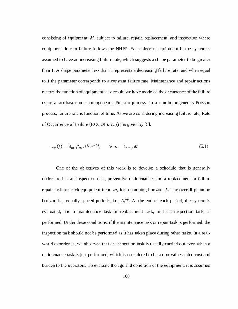
160
consisting of equipment, 𝑀, subject to failure, repair, replacement, and inspection where
equipment time to failure follows the NHPP. Each piece of equipment in the system is
assumed to have an increasing failure rate, which suggests a shape parameter to be greater
than 1. A shape parameter less than 1 represents a decreasing failure rate, and when equal
to 1 the parameter corresponds to a constant failure rate. Maintenance and repair actions
restore the function of equipment; as a result, we have modeled the occurrence of the failure
using a stochastic non-homogeneous Poisson process. In a non-homogeneous Poisson
process, failure rate is function of time. As we are considering increasing failure rate, Rate
of Occurrence of Failure (ROCOF), 𝜈𝑚(𝑡) is given by [5],
𝜈𝑚(𝑡) = 𝜆𝑚. 𝛽𝑚 . 𝑡(𝛽𝑚−1), ∀ 𝑚 = 1, … , 𝑀 (5.1)
One of the objectives of this work is to develop a schedule that is generally
understood as an inspection task, preventive maintenance, and a replacement or failure
repair task for each equipment item, 𝑚, for a planning horizon, 𝐿. The overall planning
horizon has equally spaced periods, i.e., 𝐿/𝑇. At the end of each period, the system is
evaluated, and a maintenance task or replacement task, or least inspection task, is
performed. Under these conditions, if the maintenance task or repair task is performed, the
inspection task should not be performed as it has taken place during other tasks. In a real-
world experience, we observed that an inspection task is usually carried out even when a
maintenance task is just performed, which is considered to be a non-value-added cost and
burden to the operators. To evaluate the age and condition of the equipment, it is assumed
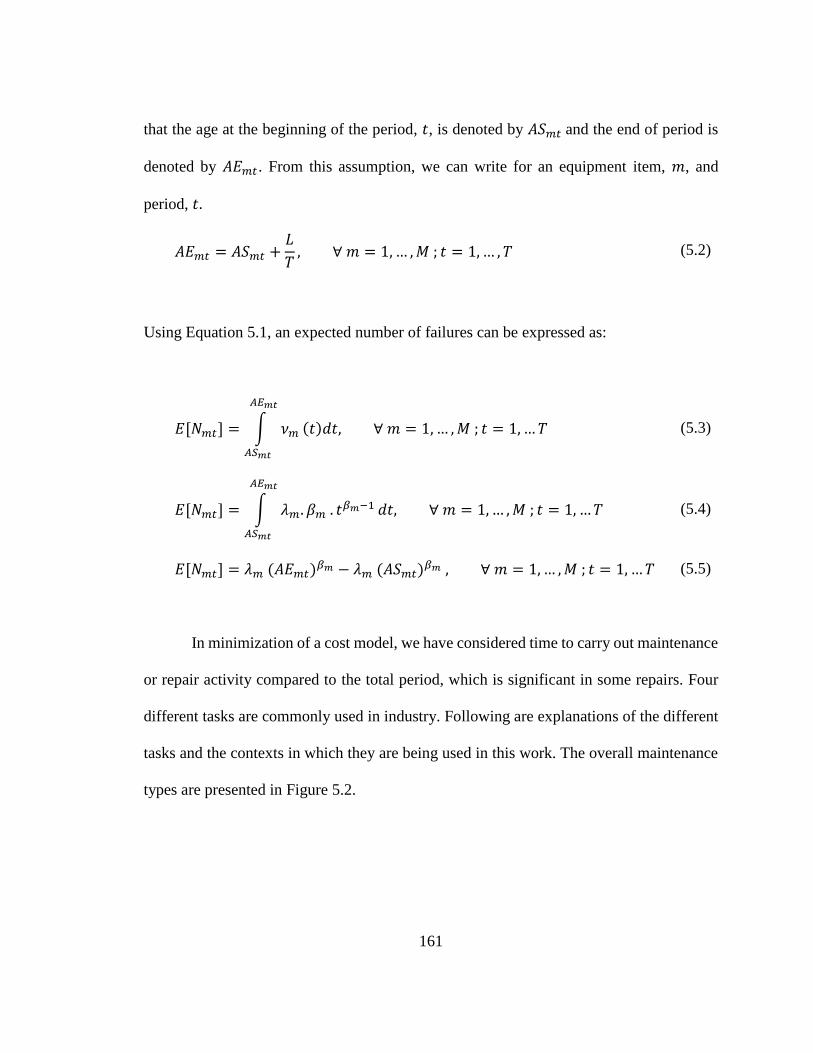
161
that the age at the beginning of the period, 𝑡, is denoted by 𝐴𝑆𝑚𝑡 and the end of period is
denoted by 𝐴𝐸𝑚𝑡. From this assumption, we can write for an equipment item, 𝑚, and
period, 𝑡.
𝐴𝐸𝑚𝑡 = 𝐴𝑆𝑚𝑡 +𝐿
𝑇, ∀ 𝑚 = 1, … , 𝑀 ; 𝑡 = 1, … , 𝑇 (5.2)
Using Equation 5.1, an expected number of failures can be expressed as:
𝐸[𝑁𝑚𝑡] = ∫ 𝜈𝑚
𝐴𝐸𝑚𝑡
𝐴𝑆𝑚𝑡
(𝑡)𝑑𝑡, ∀ 𝑚 = 1, … , 𝑀 ; 𝑡 = 1, … 𝑇 (5.3)
𝐸[𝑁𝑚𝑡] = ∫ 𝜆𝑚. 𝛽𝑚 . 𝑡𝛽𝑚−1
𝐴𝐸𝑚𝑡
𝐴𝑆𝑚𝑡
𝑑𝑡, ∀ 𝑚 = 1, … , 𝑀 ; 𝑡 = 1, … 𝑇 (5.4)
𝐸[𝑁𝑚𝑡] = 𝜆𝑚 (𝐴𝐸𝑚𝑡)𝛽𝑚 − 𝜆𝑚 (𝐴𝑆𝑚𝑡)𝛽𝑚 , ∀ 𝑚 = 1, … , 𝑀 ; 𝑡 = 1, … 𝑇 (5.5)
In minimization of a cost model, we have considered time to carry out maintenance
or repair activity compared to the total period, which is significant in some repairs. Four
different tasks are commonly used in industry. Following are explanations of the different
tasks and the contexts in which they are being used in this work. The overall maintenance
types are presented in Figure 5.2.
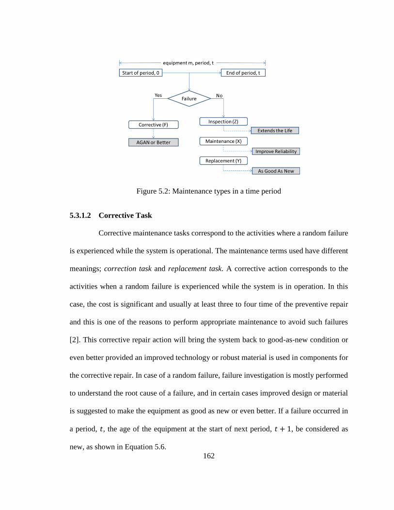
162
Figure 5.2: Maintenance types in a time period
5.3.1.2 Corrective Task
Corrective maintenance tasks correspond to the activities where a random failure
is experienced while the system is operational. The maintenance terms used have different
meanings; correction task and replacement task. A corrective action corresponds to the
activities when a random failure is experienced while the system is in operation. In this
case, the cost is significant and usually at least three to four time of the preventive repair
and this is one of the reasons to perform appropriate maintenance to avoid such failures
[2]. This corrective repair action will bring the system back to good-as-new condition or
even better provided an improved technology or robust material is used in components for
the corrective repair. In case of a random failure, failure investigation is mostly performed
to understand the root cause of a failure, and in certain cases improved design or material
is suggested to make the equipment as good as new or even better. If a failure occurred in
a period, 𝑡, the age of the equipment at the start of next period, 𝑡 + 1, be considered as
new, as shown in Equation 5.6.

163
𝐴𝑆𝑚,𝑡+1 = 0 , ∀ 𝑚 = 1, … , 𝑀 ; 𝑡 = 1, … 𝑇 (5.6)
Corrective cost is a function of repair time, man-hour, material cost and a failure
cost factor, 𝜌𝑚. The failure cost factor (𝜌𝑚) allows for the capture of cost impact due to an
equipment breakdown. In a real plant equipment breakdown situation, we have observed
that the corrective cost is higher than other non-breakdown maintenance events. This
difference in cost is captured in the model by introducing a factor, 𝜌𝑚, which increases the
repair cost and brings it closer to real plant maintenance cost. This factor depends upon
different critical parameters, i.e., equipment history, size, crew usage, and production lost.
We estimated this factor using the above parameters for each piece of equipment. The
difference in 𝜌𝑚 is justified by the variation in different parameters for each equipment
item. Mathematically, this can be written as:
𝐶𝐹𝑚 = 𝜌𝑚 × 𝐶𝑅𝑚, ∀ 𝑚 = 1, … , 𝑀 (5.7)
𝐶𝐹𝑚 = 𝜌𝑚(𝑇𝐹𝑚 × 𝐶𝐿𝐹𝑚 + 𝐶𝑀𝑇𝑚), ∀ 𝑚 = 1, … , 𝑀 (5.8)
As the cost of material does not have an impact on schedule, to make it simple,
material cost is removed from Equation 5.8, which becomes:
𝐶𝐹𝑚 = 𝜌𝑚(𝑇𝐹𝑚 × 𝐶𝐿𝐹𝑚), ∀ 𝑚 = 1, … , 𝑀 (5.9)

164
5.3.1.3 Inspection Task
Inspection task and operator task are synonymously used in industry. It is referred
to the task where plant operators evaluate the condition of the equipment by visual
inspection and take appropriate action during the daily routine rounds. The earlier concept
of a “do-nothing” operator is fading even with the availability of predictive technologies
such as condition monitoring tools. In reality, this maintenance activity provides plant
operations with the confidence that the equipment is running in an acceptable condition.
This task does not significantly improve the condition of equipment but rather helps avoid
faster degradation of the equipment as shown in Figure 5.3. The conceptual background of
this approach is adopted from a similar concept for failure rate by Moghaddam and Usher
[5]. We have extended the concept to reliability under different maintenance actions.
During the inspection phase, a slight change in reliability occurs due to the equipment time
in service. Reliability depends on the time and failure rate, so by performing inspection
and some minor tasks we maintained the equipment condition, although there was a slight
change in reliability due to the effect of aging. In conclusion, inspection helps keep
machines in a reliable running condition over a long time period. For example, if an
operator notices an abnormal sound from equipment, a necessary action will be taken as
soon as possible by the operator, such as topping up the grease in a bearing or tightening a
bolt. Similarly, if an operator sees a slight leak, an action can be taken to avoid machine
failure and degradation caused by insufficient lubrication. There is minimal physical work
performed on the system, but the benefits are considerable both in terms of cost and
equipment life. Due to this reason, most of the companies have added such tasks in operator
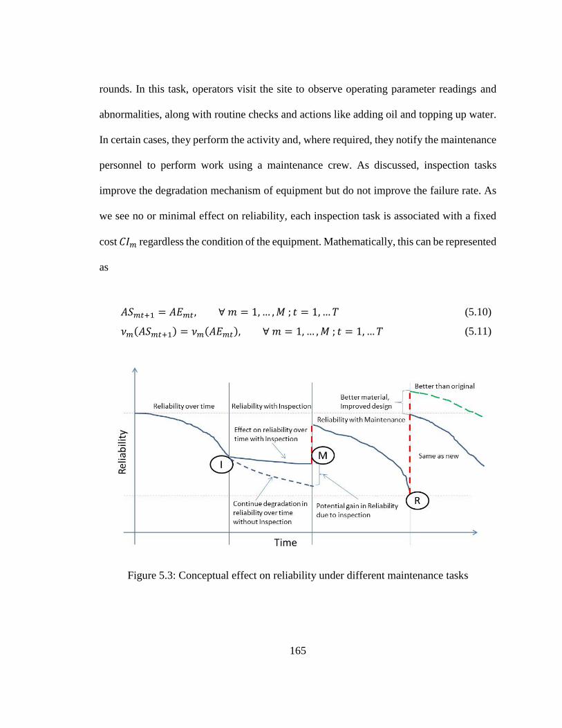
165
rounds. In this task, operators visit the site to observe operating parameter readings and
abnormalities, along with routine checks and actions like adding oil and topping up water.
In certain cases, they perform the activity and, where required, they notify the maintenance
personnel to perform work using a maintenance crew. As discussed, inspection tasks
improve the degradation mechanism of equipment but do not improve the failure rate. As
we see no or minimal effect on reliability, each inspection task is associated with a fixed
cost 𝐶𝐼𝑚 regardless the condition of the equipment. Mathematically, this can be represented
as
𝐴𝑆𝑚𝑡+1 = 𝐴𝐸𝑚𝑡 , ∀ 𝑚 = 1, … , 𝑀 ; 𝑡 = 1, … 𝑇 (5.10)
𝜈𝑚(𝐴𝑆𝑚𝑡+1) = 𝜈𝑚(𝐴𝐸𝑚𝑡), ∀ 𝑚 = 1, … , 𝑀 ; 𝑡 = 1, … 𝑇 (5.11)
Figure 5.3: Conceptual effect on reliability under different maintenance tasks

166
As discussed earlier, an inspection task improves the degradation mechanism of
equipment and extends the useful life of equipment, which can be written mathematically
as follows:
𝐶𝐼𝑚 = (𝑇𝐼𝑚 × 𝐶𝐿𝐼𝑚), ∀ 𝑚 = 1, … , 𝑀 ; 𝑡 = 1, … 𝑇 (5.12)
5.3.1.4 Maintenance Tasks
Under certain conditions, preventive maintenance is required to ensure smooth
operation of equipment to improve the overall availability and reliability of the plant. In
this research, maintenance and preventive maintenance is synonymously used, which helps
to improve the condition for future periods. Preventive maintenance improves conditions,
but it can also negatively influence the condition of equipment because of improper
maintenance. To include the impact of maintenance on the condition of the equipment, a
term 𝛼 is introduced [5]. Maintenance action during a period, 𝑡, improves the failure rate.
The value of 𝛼 ranges from 0 to 1; with 0 indicating that maintenance brought the
equipment back to “good-as-new” condition and 1 indicating that the equipment condition
is as “bad-as-old.” The effect of maintenance tasks on the condition of the equipment can
be written as follows:
𝐴𝑆𝑚𝑡+1 = 𝛼𝑚. 𝐴𝐸𝑚𝑡 , ∀ 𝑚 = 1, … , 𝑀 ; 𝑡 = 1, … 𝑇 (5.13)
The maintenance cost of an activity can be written as follows:

167
𝐶𝑀𝑚 = (𝑇𝑀𝑚 × 𝐶𝐿𝑀𝑚), ∀ 𝑚 = 1, … , 𝑀 ; 𝑡 = 1, … 𝑇 (5.14)
5.3.1.5 Replacement Task
One of the maintenance actions to ensure equipment reliability and availability
throughout the equipment life-cycle is replacement tasks. In a replacement task, the
equipment is refurbished or completely overhauled during a period of time, 𝑡, and the
system is considered as “good-as-new.” This replacement task is required to avoid
catastrophic random failures where the component of equipment is operating in a wear-out
region. All degraded components, like seals, bearings, and other major components are
replaced with new and improved components. The replacement is based on the historical
estimated life of the component or can be identified using condition monitoring techniques,
i.e., lubrication analysis, vibration data analysis, etc. In the real world, this replacement
activity is sometimes performed under the domain of opportunistic maintenance; for
example, if there is a planned shutdown of a processing unit, this task can be performed to
avoid the risk of failure during normal operation based on the condition of equipment. The
replacement task brings the equipment back to new condition or even improves the
condition where existing components have been replaced with new improved design or
material for the next period. For example, if a repair is performed at the end of a period, 𝑡,
the system is considered new for the next period, 𝑡 + 1.
𝐴𝑆𝑚𝑡+1 = 0, ∀ 𝑚 = 1, … , 𝑀 ; 𝑡 = 1, … 𝑇 (5.15)

168
Replacement cost can be estimated using Equation 5.17; while the material cost is
independent of the maintenance schedule so we take it out for schedule optimization, per
the following formula:
𝐶𝑅𝑚 = (𝑇𝑅𝑚 × 𝐶𝐿𝑅𝑚 + 𝐶𝑀𝑇𝑚), ∀ 𝑚 = 1, … , 𝑀 (5.16)
𝐶𝑅𝑚 = (𝑇𝑅𝑚 × 𝐶𝐿𝑅𝑚), ∀ 𝑚 = 1, … , 𝑀 (5.17)
5.3.2 Equipment Risk Index (ERI)
The Equipment Risk Index is a quantitative measure to estimate the importance
or criticality of equipment in an operating plant. Many qualitative and quantitative methods
are available to define and establish risk. The risk in general is the probability of an event
and its consequence as suggested in Equation 5.18. The consequences can be classified
based on different categories, which are considered important in a business such as safety
and health, production lost, and the operating history of the equipment. In this work, the
main objective of risk categorization is to establish an ERI, which can be used as a basis to
prioritize maintenance.
𝐸𝑞𝑢𝑖𝑝𝑚𝑒𝑛𝑡 𝑅𝑖𝑠𝑘 𝐼𝑛𝑑𝑒𝑥 = 𝑃𝑟𝑜𝑏𝑎𝑏𝑖𝑙𝑖𝑡𝑦 𝑜𝑓 𝐹𝑎𝑖𝑙𝑢𝑟𝑒 × 𝐶𝑜𝑛𝑠𝑒𝑞𝑢𝑒𝑛𝑐𝑒 (5.18)
The risk categorization also helps to give due importance to equipment,
prioritization of maintenance work, managing spare parts, and other related activities. A
similar concept has been used in an earlier work [4] to establish equipment risk, but that
was mainly to simplify the system based on equipment criticality. In this work, ERI is more

169
useful in maintenance prioritization. In general, there are three categories of risk, which
are high, medium and low. The ERI can be effectively used to prioritize maintenance based
on the equipment unavailability consequences rather than handling them with some other
criteria.
5.3.3 Formulation of Reliability Constraint
The objective in this formulation is minimizing cost by optimizing the
maintenance schedule and ensuring a certain level of system reliability is achieved. The
system under study is an absorption system in a gas plant and equipment are operating in
series. The system contains the static equipment, i.e., vessels and columns and rotating
machines. The scope of this problem formulation is based on optimization of the
maintenance schedule for rotating equipment and motorized valves. Static equipment is
generally subject to regulatory compliance for inspection where optimization can suggest
violation of regulatory requirements and guidelines. To develop the system reliability
constraint, we have assumed the failure follows increasing failure pattern. As discussed
earlier, the rate of failure of occurrence for repairable a system follows NHPP, so the failure
rate is replaced with ROCOF. The formulation of system reliability is presented as,
𝑅𝑚𝑡 = 𝑒−𝐸[𝑁𝑚𝑡] , ∀ 𝑚 = 1, … , 𝑀 ; 𝑡 = 1, … 𝑇 (5.19)
where, the failure rate is replaced with the ROCOF function,
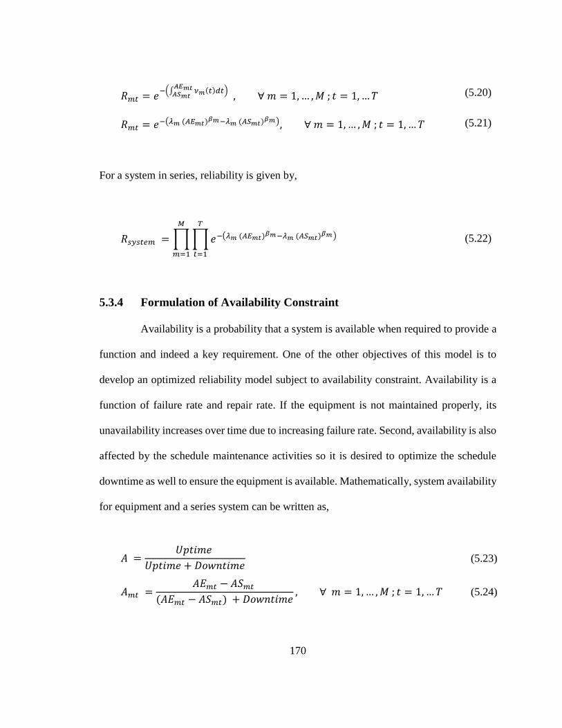
170
𝑅𝑚𝑡 = 𝑒−(∫ 𝜈𝑚
𝐴𝐸𝑚𝑡𝐴𝑆𝑚𝑡
(𝑡)𝑑𝑡) , ∀ 𝑚 = 1, … , 𝑀 ; 𝑡 = 1, … 𝑇 (5.20)
𝑅𝑚𝑡 = 𝑒−(𝜆𝑚 (𝐴𝐸𝑚𝑡)𝛽𝑚−𝜆𝑚 (𝐴𝑆𝑚𝑡)𝛽𝑚), ∀ 𝑚 = 1, … , 𝑀 ; 𝑡 = 1, … 𝑇 (5.21)
For a system in series, reliability is given by,
𝑅𝑠𝑦𝑠𝑡𝑒𝑚 = ∏ ∏ 𝑒−(𝜆𝑚 (𝐴𝐸𝑚𝑡)𝛽𝑚−𝜆𝑚 (𝐴𝑆𝑚𝑡)𝛽𝑚)
𝑇
𝑡=1
𝑀
𝑚=1
(5.22)
5.3.4 Formulation of Availability Constraint
Availability is a probability that a system is available when required to provide a
function and indeed a key requirement. One of the other objectives of this model is to
develop an optimized reliability model subject to availability constraint. Availability is a
function of failure rate and repair rate. If the equipment is not maintained properly, its
unavailability increases over time due to increasing failure rate. Second, availability is also
affected by the schedule maintenance activities so it is desired to optimize the schedule
downtime as well to ensure the equipment is available. Mathematically, system availability
for equipment and a series system can be written as,
𝐴 =𝑈𝑝𝑡𝑖𝑚𝑒
𝑈𝑝𝑡𝑖𝑚𝑒 + 𝐷𝑜𝑤𝑛𝑡𝑖𝑚𝑒 (5.23)
𝐴𝑚𝑡 =𝐴𝐸𝑚𝑡 − 𝐴𝑆𝑚𝑡
(𝐴𝐸𝑚𝑡 − 𝐴𝑆𝑚𝑡) + 𝐷𝑜𝑤𝑛𝑡𝑖𝑚𝑒, ∀ 𝑚 = 1, … , 𝑀 ; 𝑡 = 1, … 𝑇 (5.24)

171
𝐴𝑚𝑡
=𝐴𝐸𝑚𝑡 − 𝐴𝑆𝑚𝑡
(𝐴𝐸𝑚𝑡 − 𝐴𝑆𝑚𝑡) + 𝑇𝐹𝑚[𝜆𝑚 (𝐴𝐸𝑚𝑡)𝛽𝑚 − 𝜆𝑚 (𝐴𝑆𝑚𝑡)𝛽𝑚] + (𝑇𝑀𝑚 . 𝑋𝑚𝑡 + 𝑇𝑅𝑚 . 𝑌𝑚𝑡),
∀ 𝑚 = 1, … , 𝑀 ; 𝑡 = 1, … 𝑇
(5.25)
𝐴𝑠𝑦𝑠𝑡𝑒𝑚
= ∏ ∏ [𝐴𝐸𝑚𝑡 − 𝐴𝑆𝑚𝑡
(𝐴𝐸𝑚𝑡 − 𝐴𝑆𝑚𝑡) + 𝑇𝐹𝑚[𝜆𝑚 (𝐴𝐸𝑚𝑡)𝛽𝑚 − 𝜆𝑚 (𝐴𝑆𝑚𝑡)𝛽𝑚] + (𝑇𝑀𝑚
. 𝑋𝑚𝑡 + 𝑇𝑅𝑚. 𝑌𝑚𝑡)]
𝑇
𝑡=1
𝑀
𝑚=1
(5.26)
5.4 Optimization Models
In this Section, three maintenance scheduling optimization models are developed.
The objective function of the first model is to minimize maintenance cost subject to
reliability constraints. The second model explores the maximization of reliability subject
to system availability constraints. The last model is based on goal programming where the
multiple criteria are used to develop maintenance schedules and the effect of weights under
different goals was observed. All pieces of equipment are in series, and a model is
developed based on the series system as shown in Figure 5.4. Details of each model are
given in the respective Sections.

172
Sweet Gas - To Next Unit
To Slop pit
Absorber
Column
Gas to Flare
Gas to Incinerator
Ant-foam
Injection Pump
Drain Drum
Solvent
Condensate
Sour Feed Gas
Circulation
PumpsHP Flash
DrumLP Flash
Drum
Lean Solvent
Sour GasSour Gas
HP Recontactor LP Recontactor
Pump A
Pump B
Pump A
Pump B
Washing
Column
From Tank
Rich Solvent
Pump A
Skimming Drains
Rich Solvent
Pumps
Pump A
Pump B
Pump A
Pump B
Skim Oil
Pumps
Rich Solvent
To Flare
HP Solvent
Wet Sweet
Gas
To Exchangers
Figure 5.4: Overall Schematic of a Gas Absorption System [4]
5.4.1 Minimize Total Maintenance Cost subject to Reliability Constraints
In this optimization model, the objective is to minimize cost by optimizing the
maintenance schedule based on the condition or age of the equipment and ensure that the
plant meets the required reliability targets. All the equipment items are in series, and the
model is developed based on the series as shown in Figure 5.4. Formulation of the total
cost model is subject to the reliability constraints given below:
𝑀𝑖𝑛𝑖𝑚𝑖𝑧𝑒 𝑇𝑜𝑡𝑎𝑙 𝐶𝑜𝑠𝑡
= ∑ ∑[𝐹𝑎𝑖𝑙𝑢𝑟𝑒 𝐶𝑜𝑠𝑡 + 𝑀𝑎𝑖𝑛𝑡𝑒𝑛𝑎𝑛𝑐𝑒 𝐶𝑜𝑠𝑡]
𝑇
𝑡=1
𝑀
𝑚=1
(5.27)

173
= ∑ ∑[𝐶𝐹𝑚. 𝐸[𝑁𝑚𝑡]+{(𝐶𝑀𝑚. 𝑋𝑚𝑡) + (𝐶𝑅𝑚 . 𝑌𝑚𝑡) + (𝐶𝐼𝑚. 𝑍𝑚𝑡)}]
𝑇
𝑡=1
𝑀
𝑚=1
𝑆𝑢𝑏𝑗𝑒𝑐𝑡 𝑡𝑜:
𝐴𝑆𝑚1 = 0, ∀ 𝑚 = 1, … , 𝑀 (5.28)
𝐴𝑆𝑚𝑡 = (𝐴𝐸𝑚𝑡−1)𝑍𝑚𝑡 + (𝛼𝑚. 𝐴𝐸𝑚𝑡−1). 𝑋𝑚𝑡,
∀ 𝑚 = 1, … , 𝑀 ; 𝑡 = 2, … 𝑇 (5.29)
𝐴𝐸𝑚𝑡 = 𝐴𝑆𝑚𝑡 +𝐿
𝑇, ∀ 𝑚 = 1, … , 𝑀 ; 𝑡 = 1, … 𝑇 (5.30)
∏ ∏ 𝑒−(𝜆𝑚 (𝐴𝐸𝑚𝑡)𝛽𝑚−𝜆𝑚 (𝐴𝑆𝑚𝑡)𝛽𝑚)
𝑇
𝑡=1
𝑀
𝑚=1
≥ 𝑅𝑡𝑎𝑟𝑔𝑒𝑡 (5.31)
𝑋𝑚𝑡 + 𝑌𝑚𝑡 + 𝑍𝑚𝑡 = 1 (5.32)
𝐴𝑆𝑚𝑡, 𝐴𝐸𝑚𝑡 ≥ 0 (5.33)
𝑋𝑚𝑡, 𝑌𝑚𝑡, 𝑍𝑚𝑡 = {0, 1} (5.34)
5.4.2 Maximize System Reliability subject to Availability Constraints
In this optimization model, the objective is to maximize reliability subject to
availability targets. All the equipment items are in series, and the model is developed based
on the series shown in Figure 5.4. Formulation of the maximization of reliability is subject
to the availability constraint given below:
𝑀𝑎𝑥𝑖𝑚𝑖𝑧𝑒 𝑅𝑒𝑙𝑖𝑎𝑏𝑖𝑙𝑖𝑡𝑦 = ∏ ∏ 𝑒−(𝜆𝑚 (𝐴𝐸𝑚𝑡)𝛽𝑚−𝜆𝑚 (𝐴𝑆𝑚𝑡)𝛽𝑚)
𝑇
𝑡=1
𝑀
𝑚=1
(5.35)
𝑆𝑢𝑏𝑗𝑒𝑐𝑡 𝑡𝑜:

174
𝐴𝑆𝑚1 = 0, ∀ 𝑚 = 1, … , 𝑀 (5.36)
𝐴𝑆𝑚𝑡 = (𝐴𝐸𝑚𝑡−1)𝑍𝑚𝑡 + (𝛼𝑚. 𝐴𝐸𝑚𝑡−1). 𝑋𝑚𝑡,
∀ 𝑚 = 1, … , 𝑀 ; 𝑡 = 2, … 𝑇 (5.37)
𝐴𝐸𝑚𝑡 = 𝐴𝑆𝑚𝑡 +𝐿
𝑇, ∀ 𝑚 = 1, … , 𝑀 ; 𝑡 = 1, … 𝑇 (5.38)
∏ ∏ [𝐴𝐸𝑚𝑡 − 𝐴𝑆𝑚𝑡
(𝐴𝐸𝑚𝑡 − 𝐴𝑆𝑚𝑡) + 𝑇𝐹𝑚[𝜆𝑚 (𝐴𝐸𝑚𝑡)𝛽𝑚 − 𝜆𝑚 (𝐴𝑆𝑚𝑡)𝛽𝑚] + (𝑇𝑀𝑚
. 𝑋𝑚𝑡 + 𝑇𝑅𝑚. 𝑌𝑚𝑡)]
𝑇
𝑡=1
𝑀
𝑚=1
≥ 𝐴𝑡𝑎𝑟𝑔𝑒𝑡
(5.39)
𝑋𝑚𝑡 + 𝑌𝑚𝑡 + 𝑍𝑚𝑡 = 1 (5.40)
𝐴𝑆𝑚𝑡, 𝐴𝐸𝑚𝑡 ≥ 0 (5.41)
𝑋𝑚𝑡, 𝑌𝑚𝑡, 𝑍𝑚𝑡 = {0, 1} (5.42)
5.4.3 Minimization of Deviation from Goals using Goal Programming
Goal programming is an effective tool in multi-criteria decision making. It is an
extension of linear programming to handle multiple optimization objectives. It is an
optimization program and works with a given target value and importance to the decision
variables. Deviations are minimized from goals using an achievement function. All three
criteria were used with different goals and weights to come up with strategies. Formulation
of the goal programming objective function, which is minimization of summation of
deviation from designated goals, is given below:
𝑀𝑖𝑛𝑖𝑚𝑖𝑧𝑒 𝑤𝑒𝑖𝑔ℎ𝑡𝑒𝑑 𝑑𝑒𝑣𝑖𝑎𝑡𝑖𝑜𝑛𝑠 = 𝑤1𝑑1+ + 𝑤2𝑑2
−+ 𝑤3𝑑3− (5.43)
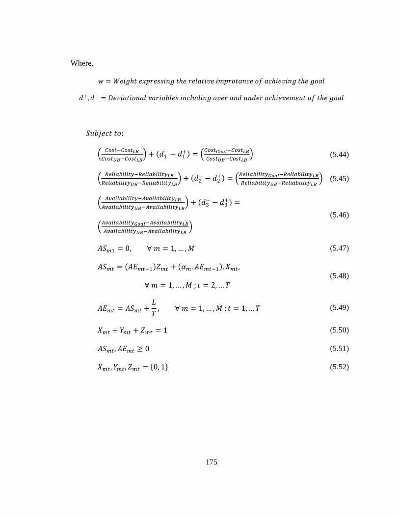
175
Where,
𝑤 = 𝑊𝑒𝑖𝑔ℎ𝑡 𝑒𝑥𝑝𝑟𝑒𝑠𝑠𝑖𝑛𝑔 𝑡ℎ𝑒 𝑟𝑒𝑙𝑎𝑡𝑖𝑣𝑒 𝑖𝑚𝑝𝑟𝑜𝑡𝑎𝑛𝑐𝑒 𝑜𝑓 𝑎𝑐ℎ𝑖𝑒𝑣𝑖𝑛𝑔 𝑡ℎ𝑒 𝑔𝑜𝑎𝑙
𝑑+, 𝑑− = 𝐷𝑒𝑣𝑖𝑎𝑡𝑖𝑜𝑛𝑎𝑙 𝑣𝑎𝑟𝑖𝑎𝑏𝑙𝑒𝑠 𝑖𝑛𝑐𝑙𝑢𝑑𝑖𝑛𝑔 𝑜𝑣𝑒𝑟 𝑎𝑛𝑑 𝑢𝑛𝑑𝑒𝑟 𝑎𝑐ℎ𝑖𝑒𝑣𝑒𝑚𝑒𝑛𝑡 𝑜𝑓 𝑡ℎ𝑒 𝑔𝑜𝑎𝑙
𝑆𝑢𝑏𝑗𝑒𝑐𝑡 𝑡𝑜:
(𝐶𝑜𝑠𝑡−𝐶𝑜𝑠𝑡𝐿𝐵
𝐶𝑜𝑠𝑡𝑈𝐵−𝐶𝑜𝑠𝑡𝐿𝐵) + (𝑑1
− − 𝑑1+) = (
𝐶𝑜𝑠𝑡𝐺𝑜𝑎𝑙−𝐶𝑜𝑠𝑡𝐿𝐵
𝐶𝑜𝑠𝑡𝑈𝐵−𝐶𝑜𝑠𝑡𝐿𝐵) (5.44)
(𝑅𝑒𝑙𝑖𝑎𝑏𝑖𝑙𝑖𝑡𝑦−𝑅𝑒𝑙𝑖𝑎𝑏𝑖𝑙𝑖𝑡𝑦𝐿𝐵
𝑅𝑒𝑙𝑖𝑎𝑏𝑖𝑙𝑖𝑡𝑦𝑈𝐵−𝑅𝑒𝑙𝑖𝑎𝑏𝑖𝑙𝑖𝑡𝑦𝐿𝐵) + (𝑑2
− − 𝑑2+) = (
𝑅𝑒𝑙𝑖𝑎𝑏𝑖𝑙𝑖𝑡𝑦𝐺𝑜𝑎𝑙−𝑅𝑒𝑙𝑖𝑎𝑏𝑖𝑙𝑖𝑡𝑦𝐿𝐵
𝑅𝑒𝑙𝑖𝑎𝑏𝑖𝑙𝑖𝑡𝑦𝑈𝐵−𝑅𝑒𝑙𝑖𝑎𝑏𝑖𝑙𝑖𝑡𝑦𝐿𝐵) (5.45)
(𝐴𝑣𝑎𝑖𝑙𝑎𝑏𝑖𝑙𝑖𝑡𝑦−𝐴𝑣𝑎𝑖𝑙𝑎𝑏𝑖𝑙𝑖𝑡𝑦𝐿𝐵
𝐴𝑣𝑎𝑖𝑙𝑎𝑏𝑖𝑙𝑖𝑡𝑦𝑈𝐵−𝐴𝑣𝑎𝑖𝑙𝑎𝑏𝑖𝑙𝑖𝑡𝑦𝐿𝐵) + (𝑑3
− − 𝑑3+) =
(𝐴𝑣𝑎𝑖𝑙𝑎𝑏𝑖𝑙𝑖𝑡𝑦𝐺𝑜𝑎𝑙−𝐴𝑣𝑎𝑖𝑙𝑎𝑏𝑖𝑙𝑖𝑡𝑦𝐿𝐵
𝐴𝑣𝑎𝑖𝑙𝑎𝑏𝑖𝑙𝑖𝑡𝑦𝑈𝐵−𝐴𝑣𝑎𝑖𝑙𝑎𝑏𝑖𝑙𝑖𝑡𝑦𝐿𝐵)
(5.46)
𝐴𝑆𝑚1 = 0, ∀ 𝑚 = 1, … , 𝑀 (5.47)
𝐴𝑆𝑚𝑡 = (𝐴𝐸𝑚𝑡−1)𝑍𝑚𝑡 + (𝛼𝑚. 𝐴𝐸𝑚𝑡−1). 𝑋𝑚𝑡,
∀ 𝑚 = 1, … , 𝑀 ; 𝑡 = 2, … 𝑇 (5.48)
𝐴𝐸𝑚𝑡 = 𝐴𝑆𝑚𝑡 +𝐿
𝑇, ∀ 𝑚 = 1, … , 𝑀 ; 𝑡 = 1, … 𝑇 (5.49)
𝑋𝑚𝑡 + 𝑌𝑚𝑡 + 𝑍𝑚𝑡 = 1 (5.50)
𝐴𝑆𝑚𝑡, 𝐴𝐸𝑚𝑡 ≥ 0 (5.51)
𝑋𝑚𝑡, 𝑌𝑚𝑡, 𝑍𝑚𝑡 = {0, 1} (5.52)
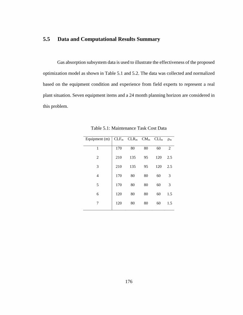
176
5.5 Data and Computational Results Summary
Gas absorption subsystem data is used to illustrate the effectiveness of the proposed
optimization model as shown in Table 5.1 and 5.2. The data was collected and normalized
based on the equipment condition and experience from field experts to represent a real
plant situation. Seven equipment items and a 24 month planning horizon are considered in
this problem.
Table 5.1: Maintenance Task Cost Data
Equipment (m) CLFm CLRm CMm CLIm ρm
1 170 80 80 60 2
2 210 135 95 120 2.5
3 210 135 95 120 2.5
4 170 80 80 60 3
5 170 80 80 60 3
6 120 80 80 60 1.5
7 120 80 80 60 1.5
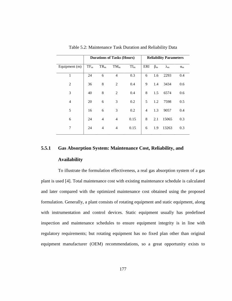
177
Table 5.2: Maintenance Task Duration and Reliability Data
Durations of Tasks (Hours) Reliability Parameters
Equipment (m) TFm TRm TMm TIm ERI βm λm αm
1 24 6 4 0.3 6 1.6 2293 0.4
2 36 8 2 0.4 9 1.4 3434 0.6
3 40 8 2 0.4 8 1.5 6574 0.6
4 20 6 3 0.2 5 1.2 7598 0.5
5 16 6 3 0.2 4 1.3 9057 0.4
6 24 4 4 0.15 8 2.1 15065 0.3
7 24 4 4 0.15 6 1.9 13263 0.3
5.5.1 Gas Absorption System: Maintenance Cost, Reliability, and
Availability
To illustrate the formulation effectiveness, a real gas absorption system of a gas
plant is used [4]. Total maintenance cost with existing maintenance schedule is calculated
and later compared with the optimized maintenance cost obtained using the proposed
formulation. Generally, a plant consists of rotating equipment and static equipment, along
with instrumentation and control devices. Static equipment usually has predefined
inspection and maintenance schedules to ensure equipment integrity is in line with
regulatory requirements; but rotating equipment has no fixed plan other than original
equipment manufacturer (OEM) recommendations, so a great opportunity exists to
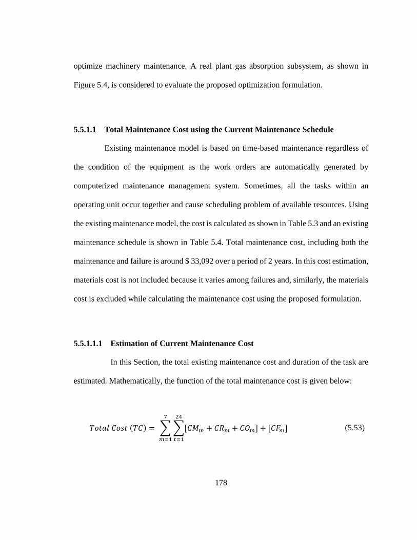
178
optimize machinery maintenance. A real plant gas absorption subsystem, as shown in
Figure 5.4, is considered to evaluate the proposed optimization formulation.
5.5.1.1 Total Maintenance Cost using the Current Maintenance Schedule
Existing maintenance model is based on time-based maintenance regardless of
the condition of the equipment as the work orders are automatically generated by
computerized maintenance management system. Sometimes, all the tasks within an
operating unit occur together and cause scheduling problem of available resources. Using
the existing maintenance model, the cost is calculated as shown in Table 5.3 and an existing
maintenance schedule is shown in Table 5.4. Total maintenance cost, including both the
maintenance and failure is around $ 33,092 over a period of 2 years. In this cost estimation,
materials cost is not included because it varies among failures and, similarly, the materials
cost is excluded while calculating the maintenance cost using the proposed formulation.
5.5.1.1.1 Estimation of Current Maintenance Cost
In this Section, the total existing maintenance cost and duration of the task are
estimated. Mathematically, the function of the total maintenance cost is given below:
𝑇𝑜𝑡𝑎𝑙 𝐶𝑜𝑠𝑡 (𝑇𝐶) = ∑ ∑[𝐶𝑀𝑚
24
𝑡=1
+ 𝐶𝑅𝑚 + 𝐶𝑂𝑚] + [𝐶𝐹𝑚]
7
𝑚=1
(5.53)
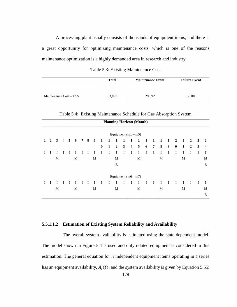
179
A processing plant usually consists of thousands of equipment items, and there is
a great opportunity for optimizing maintenance costs, which is one of the reasons
maintenance optimization is a highly demanded area in research and industry.
Table 5.3: Existing Maintenance Cost
Total Maintenance Event Failure Event
Maintenance Cost – US$ 33,092 29,592 3,500
Table 5.4: Existing Maintenance Schedule for Gas Absorption System
Planning Horizon (Month)
Equipment (m1 – m5)
1 2 3 4 5 6 7 8 9 1
0
1
1
1
2
1
3
1
4
1
5
1
6
1
7
1
8
1
9
2
0
2
1
2
2
2
3
2
4
I I I I I I I I I I I I I I I I I I I I I I I I
M M M M M M M M
R R
Equipment (m6 – m7)
I I I I I I I I I I I I I I I I I I I I I I I I
M M M M M M M M
R
5.5.1.1.2 Estimation of Existing System Reliability and Availability
The overall system availability is estimated using the state dependent model.
The model shown in Figure 5.4 is used and only related equipment is considered in this
estimation. The general equation for 𝑛 independent equipment items operating in a series
has an equipment availability, 𝐴𝑖(𝑡); and the system availability is given by Equation 5.55:

180
𝐴𝑠(𝑡) = ∏ 𝐴𝑖
𝑛
𝑖=1
(𝑡) (5.54)
Where,
𝐴𝑖 = 𝐴𝑣𝑖𝑎𝑙𝑎𝑏𝑖𝑙𝑖𝑡𝑦 𝑜𝑓 𝑠𝑦𝑠𝑡𝑒𝑚 𝑖
In general, availability of a system can be written as,
𝐴𝑖 = ∑ 𝑃𝑖
.
𝑎𝑙𝑙 𝑠𝑢𝑐𝑒𝑠𝑠 𝑠𝑎𝑡𝑒𝑠 𝑖
(5.55)
Where,
𝑃𝑖 = 𝑃𝑟𝑜𝑏𝑎𝑏𝑖𝑙𝑖𝑡𝑦 𝑜𝑓 𝑠𝑦𝑠𝑡𝑒𝑚 𝑖𝑛 𝑠𝑢𝑐𝑐𝑒𝑠𝑠 𝑠𝑡𝑎𝑡𝑒𝑠
Similarly, the system reliability equation for a unit having series system can be written as,
𝑅𝑆(𝑡) = ∏ 𝑅𝑖
𝑛
𝑖=1
(𝑡) (5.56)
Where,
𝑅𝑖 = 𝑅𝑒𝑙𝑖𝑎𝑏𝑖𝑙𝑖𝑡𝑦 𝑜𝑓 𝑒𝑞𝑢𝑖𝑝𝑚𝑒𝑛𝑡 𝑖
The reliability is also estimated using the simplified system as shown in Figure 5.4.
To capture the uncertainty in the failure data, a 2.5% sensitivity factor is used. These values
represent the existing availability ranging from 96.4-98.8%, whereas reliability ranges
from 92.0-94.4%, as shown in Table 5.5.
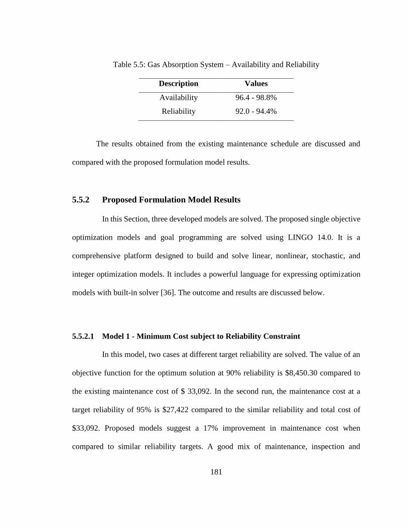
181
Table 5.5: Gas Absorption System – Availability and Reliability
Description Values
Availability 96.4 - 98.8%
Reliability 92.0 - 94.4%
The results obtained from the existing maintenance schedule are discussed and
compared with the proposed formulation model results.
5.5.2 Proposed Formulation Model Results
In this Section, three developed models are solved. The proposed single objective
optimization models and goal programming are solved using LINGO 14.0. It is a
comprehensive platform designed to build and solve linear, nonlinear, stochastic, and
integer optimization models. It includes a powerful language for expressing optimization
models with built-in solver [36]. The outcome and results are discussed below.
5.5.2.1 Model 1 - Minimum Cost subject to Reliability Constraint
In this model, two cases at different target reliability are solved. The value of an
objective function for the optimum solution at 90% reliability is $8,450.30 compared to
the existing maintenance cost of $ 33,092. In the second run, the maintenance cost at a
target reliability of 95% is $27,422 compared to the similar reliability and total cost of
$33,092. Proposed models suggest a 17% improvement in maintenance cost when
compared to similar reliability targets. A good mix of maintenance, inspection and

182
replacement tasks are observed. It can be also be concluded that by increasing the reliability
threshold the number and frequency of replacement actions increases. Tables 5.6 and 5.7
show the schedules of the optimized maintenance activities at given reliability targets.
Table 5.6: Total Maintenance Cost Subject to Reliability Constraints
Total Cost = $8450.3; Reliability = 90.0%
m Planning Horizon (Month)
1 2 3 4 5 6 7 8 9 1
0
1
1
1
2
1
3
1
4
1
5
1
6
1
7
1
8
1
9
2
0
2
1
2
2
2
3
2
4
1 I I I I I I R I I I I R I I I I R I I I I I I I
2 I I I I I I I I I I M I I M I I I I I I I I I I
3 I I I I I I I I I I I M I I I M I I I I I I I I
4 I I I I I I I I I I I I I I I I I I I I I I I I
5 I I I I I I I I I I I I I I I I I I I I I I I I
6 I I I I I I I R I I I I R I I I I R I R I I I I
7 I I I I I I I I I I R I I I I I I I R I I I I I
Table 5.7: Total Maintenance Cost Subject to Reliability Constraints
Total Cost = $ 27,422.1; Reliability = 95.0%
m Planning Horizon (Month)
1 2 3 4 5 6 7 8 9 1
0
1
1
1
2
1
3
1
4
1
5
1
6
1
7
1
8
1
9
2
0
2
1
2
2
2
3
2
4
1 I R R M R M R R R R R R I R M R R R R R R R R R
2 I I I M M M M M M I I R I M M M M M M M M M I I
3 I I I M M M I I R I I M M M M M M M M M M I I I
4 I I I I I I I I I I I I I I I I I I I I I I I I
5 I I I I I R I I I I I I R I I I I I I I I R I I
6 I I R I R I R I R I R I I R I I R I I I I I R I
7 I I I R I R I R I R I R I R I R I I I I I R I I
The ERI can be effectively utilized in the scenarios where multiple tasks are
required to be schedules, as in case of the schedule in Table 5.7. The use of the ERI in such

183
cases makes it useful for field engineers and maintenance planners to plan maintenance on
critical equipment prior to scheduling less critical equipment to avoid consequences posed
by the failure of critical equipment. Table 5.8 shows the impact of equipment criticality on
the maintenance schedule and this becomes very useful during the scheduling of a complete
unit or plant maintenance tasks.
Table 5.8: Effect of ERI on the Maintenance Schedule
Total Cost = $ 27,422.1; Reliability = 95.0%
m ERI Planning Horizon (Month)
1 2 3 4 5 6 7 8 9 1
0
1
1
1
2
1
3
1
4
1
5
1
6
1
7
1
8
1
9
2
0
2
1
2
2
2
3
2
4
2 9 I I I M M M M M M I I R I M M M M M M M M M I I
3 8 I I I M M M I I R I I M M M M M M M M M M I I I
6 8 I I R I R I R I R I R I I R I I R I I I I I R I
1 6 I R R M R M R R R R R R I R M R R R R R R R R R
7 6 I I I R I R I R I R I R I R I R I I I I I R I I
4 5 I I I I I I I I I I I I I I I I I I I I I I I I
5 4 I I I I I R I I I I I I R I I I I I I I I R I I
5.5.2.2 Model 2 - Maximize Reliability subject to Availability Constraint
In this model, two cases at different target availability are solved. The value of
the objective function, reliability, for the optimum solution at 80% availability is 90.2%.
In the second run, the value of the objective function is 89.1% at a target availability of
85%. A mix of maintenance, inspection, and replacement tasks are observed. The results
show that, with the increase in availability threshold, the system is performing more
inspections compared to maintenance and replacement task as evident in the schedules.

184
Table 5.9 and Table 5.10 show the detailed schedules of the optimized maintenance
activities at given availability targets.
Table 5.9: Maximize Reliability Subject to Availability Constraint
Reliability = 90.2%; Availability = 80.0%
m Planning Horizon (Month)
1 2 3 4 5 6 7 8 9 1
0
1
1
1
2
1
3
1
4
1
5
1
6
1
7
1
8
1
9
2
0
2
1
2
2
2
3
2
4
1 I I I I R I I I I I R I I I I I R I I I R I I I
2 I I I I I I I I I I I M I I I I I I I I I I I I
3 I I I I I I I I I I I I I I I I I I I I I I I I
4 I I I I I I I I I I I I I I I I I I I I I I I I
5 I I I I I I I I I I I I I I I I I I I I I I I I
6 I I I I I R I I I I R I I I I I R I I I I I I I
7 I I I I I I R I I I I R I I I I I I I R I I I I
Table 5.10: Maximize Reliability Subject to Availability Constraint
Reliability = 89.1%; Availability = 85.0%
m Planning Horizon (Month)
1 2 3 4 5 6 7 8 9 1
0
1
1
1
2
1
3
1
4
1
5
1
6
1
7
1
8
1
9
2
0
2
1
2
2
2
3
2
4
1 I I I I I I I R I I I I I I R I I I I R I I I I
2 I M I I I I I I I I I I I I I I I I I I I I I I
3 I I I I I I I I I I I I I I I I I I I I I I I I
4 I I I I I I I I I I I I I I I I I I I I I I I I
5 I I I I I I I I I I I I I I I I I I I I I I I I
6 I I I I I I I R I I I I I I I I R I I I I I I I
7 I I I I I I I I I R I I I I I I I I I R I I I I

185
5.5.2.3 Model 3 – Minimization of Deviation from Goals using Goal Programming
In this model, minimization of deviation, as an objective function, is developed
using a goal programming approach. Deviations are minimized from the goal using an
achievement function. All three criteria were used with different goals and weights to come
up with strategies. Table 5.11 shows the different runs with assigned goals and weights.
The goal programming model is flexible as different goals and weights can be assessed in
a dynamic way and schedules can be adjusted on the plant requirements.
Table 5.11: Goals and Weights for Goal Programming
Exp. Total Maintenance Cost Reliability Availability
E - 1 Goal 6000 1 1
Weight 1 0 0
E - 2 Goal 6000 1 1
Weight 0 1 0
E - 3 Goal 6000 1 1
Weight 0 0 1
E - 4 Goal 6000 1 1
Weight 0.5 0.4 0.1
E - 5 Goal 6000 1 1
Weight 0.3 0.6 0.1
Table 5.12 and 5.13 shows the optimized maintenance schedule. Table 5.11 shows
the results in the form of maintenance cost, reliability, and availability under predefined
goal and weights. Many required scenarios can be run by changing the weights and goals.
The maintenance cost of $7,589.5 is estimated with a reliability of 89.0% and availability
of 86.4% subject to cost, reliability, and availability weights of 0.5, 0.4, and 0.1,
respectively. The maintenance cost of $8,749.7 is estimated with a reliability of 90.3% and

186
availability of 80.3% subject to cost, reliability, and availability weights of 0.3, 0.6, and
0.1, respectively. Other scenarios can be developed and evaluated based on the business
requirements to come up with optimized maintenance schedule. The goal programming
model was solved using LINGO software to find out the optimal maintenance policy, and
cost under different weights and goals.
Table 5.12: Schedule – Weights for Cost: 0.5, Reliability: 0.4, and Availability: 0.1
E4: Total Cost = $7,589.5; Reliability = 89.0%; Availability = 86.4%
m Planning Horizon (Month)
1 2 3 4 5 6 7 8 9 1
0
1
1
1
2
1
3
1
4
1
5
1
6
1
7
1
8
1
9
2
0
2
1
2
2
2
3
2
4
1 I I I I I I I R I I I I I I I I R I I I I I I I
2 I I I I I I I I I I I I I I I I I I I I I I I I
3 I I I I I I I I I I I I I I I I I I I I I I I I
4 I I I I I I I I I I I I I I I I I I I I I I I I
5 I I I I I I I I I I I I I I I I I I I I I I I I
6 I I I I I R I I I I I I R I I I I I R I I I I I
7 I I I I I I I R I I I I I R I I I I I I I I I I
Table 5.13: Schedule – Weights for Cost: 0.3, Reliability: 0.6 and Availability: 0.1
E5: Total Cost = $8,749.7; Reliability = 90.3%; Availability = 80.3%
m Planning Horizon (Month)
1 2 3 4 5 6 7 8 9 1
0
1
1
1
2
1
3
1
4
1
5
1
6
1
7
1
8
1
9
2
0
2
1
2
2
2
3
2
4
1 I I I I I I I R I I I R I I I I R I I I I I I I
2 I I I I I I I I I I M I I M I I I I I I I I I I
3 I I I I I I I I I M I I I M I I I I I I I I I I
4 I I I I I I I I I I I I I I I I I I I I I I I I
5 I I I I I I I I I I I I I I I I I I I I I I I I
6 I I I I I I R I I I I I R I I I I I R I I I I I
7 I I I I I R I I I I R I I I I I I I R I I I I I

187
Table 5.14 summarizes the results of the goal programming model with certain
model runs, goals, and weights can be changed to evaluate the other scenarios.
Table 5.14: Summary of Results – Goal Programming
Total Maintenance Cost Reliability Availability
E - 1 5,645.9 0.810 0.977
E - 2 98,038.6 0.970 0.018
E - 3 5,645.9 0.810 0.977
E - 4 7,589.5 0.890 0.864
E - 5 8,749.7 0.903 0.803
5.6 Conclusion
This research work proposes two nonlinear mixed-integer optimization models and
a goal programming model for maintenance scheduling of a complex real plant gas
absorption system of a hydrocarbon facility. These proposed formulation attempts to
minimize cost and maximize reliability, and the goal programing model handles multiple
and conflicting objective to optimize the maintenance schedule. The proposed models have
given promising results and proved to be a useful tool to industry for handling maintenance
scheduling optimization under various constraints. The proposed model successfully
optimized the existing maintenance schedule of a gas absorption system and suggested
17% improvement in maintenance cost when compared to similar system reliability levels.
A huge maintenance cost improvement is expected, once the proposed model is applied to
a complete plant. The goal programming model provides flexibility to engineers and
188
planners to develop maintenance schedules considering different conflicting objectives.
The overall results derived from the proposed optimization models confirm the
applicability of the approach to real-world maintenance optimization problem and its
application to other asset intensive industries where maintenance is important to ensure
safety, availability, and reliability of the facilities.
In future work, the proposed formulation will be extended to solve similar problems
and compare the effectiveness of the results using multi-objective meta- heuristic
techniques.

CHAPTER 6
CONCLUSION, CONTRIBUTIONS AND FUTURE WORK
6.1 Introduction
Availability is an important measure in complex systems and applicable to many
industries, such as refineries, gas plants, power systems, and communication. It is a key
measure to have confidence in the processes used to meet requirements for meeting
production, safety, and financial targets. Availability and reliability are considered, but
both are different. High reliability on its own is not sufficient to ensure system availability.
Quick restoration of equipment back to service, essentially termed as maintainability, is
also important for maximization of availability. Different industries have different
requirements for availability to meet customer expectations. There are many ways to
maximize availability such as optimized and robust design, cost, manpower, skill level of
the maintenance crew, etc. In the communication and power sector, high availability is
obtained through redundant, highly reliable equipment, and schedule maintenance [1].
Power systems are designed for availability close to 100%, using modest reliable design
but highly redundant and perfectly maintained equipment with a sharing option. In the

process industry, availability is achieved by highly reliable equipment with low
maintainability [1]. The significance of availability in different industries makes it an
important topic for research. The need for availability improvement has motivated authors
to contribute by developing some new and novel methods to address this most desired area
of industry interest.
In this research, availability estimation and management is addressed by focusing
on different areas such as risk-based availability estimation; early fault detection; effective
equipment failure investigation; and maintenance scheduling optimization. Based on the
author’s experience, developments in these areas can significantly contribute to addressing
availability.
6.2 Research Contributions
In this thesis, an overall solution is developed to estimate and manage the
availability of complex processing systems and plants. Availability is an important factor
for companies to use to reap real benefits from monitoring and managing equipment. The
benefits of managing availability have many facets, such as high reliability, low
maintainability, optimized plant design, and cost. The need for availability estimation and
management models provides us an opportunity to work on this topic and develop tools
and models that can be used effectively to benefit different organizations and to help them
achieve their objectives. As discussed earlier, availability is a key performance parameter,
which is applicable to many industries. Availability management is a process, if managed
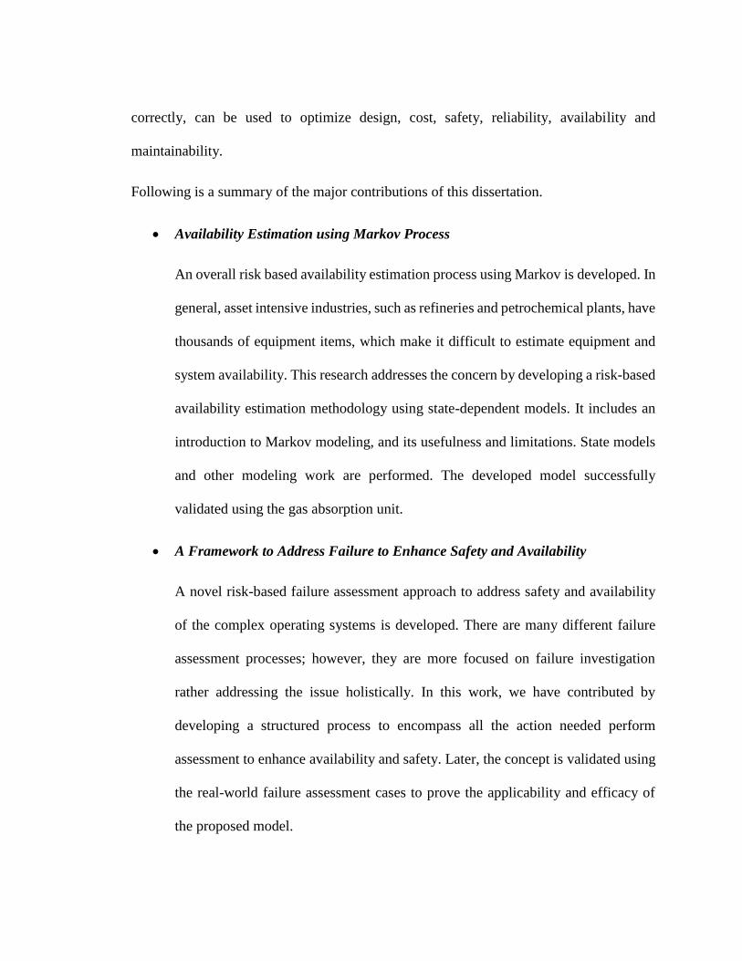
correctly, can be used to optimize design, cost, safety, reliability, availability and
maintainability.
Following is a summary of the major contributions of this dissertation.
Availability Estimation using Markov Process
An overall risk based availability estimation process using Markov is developed. In
general, asset intensive industries, such as refineries and petrochemical plants, have
thousands of equipment items, which make it difficult to estimate equipment and
system availability. This research addresses the concern by developing a risk-based
availability estimation methodology using state-dependent models. It includes an
introduction to Markov modeling, and its usefulness and limitations. State models
and other modeling work are performed. The developed model successfully
validated using the gas absorption unit.
A Framework to Address Failure to Enhance Safety and Availability
A novel risk-based failure assessment approach to address safety and availability
of the complex operating systems is developed. There are many different failure
assessment processes; however, they are more focused on failure investigation
rather addressing the issue holistically. In this work, we have contributed by
developing a structured process to encompass all the action needed perform
assessment to enhance availability and safety. Later, the concept is validated using
the real-world failure assessment cases to prove the applicability and efficacy of
the proposed model.

Fault Detection to Improve Availability using Decision Trees
As discussed earlier, availability encompasses maintainability and reliability. The
novel idea in this work was to develop algorithm using machinery data to detect
early faults prior they became threat to unscheduled downtime. Early fault detection
indeed helps improving reliability and availability, hence, ensure availability. To
detect early faults, a novel fault detection and management model is developed
using decision trees to support system availability and safety improvement.
Decision trees model is developed in MATLAB as a predictive data mining tool to
detect early faults, and their management to improve system availability. To
conclude the effectiveness of the model, the proposed model was successfully
tested to detect faults using real plant machinery vibration data.
Multi-Constrained Maintenance Scheduling Optimization
Maintenance is vital for improving the availability and reliability of the equipment
and facilities. Multi-constrained, multi-objective maintenance scheduling
optimization models are proposed using exact and optimized solutions. The model
was developed in commercial software LINGO to solve optimization problem. The
optimization problem was developed considering the time-dependent equipment
failure rate to optimize maintenance cost at different availability and reliability
levels. Different optimization scenarios were considered, such as minimization of
cost, maximization of availability and reliability etc… These models were applied
on a plant scenario to show the effectiveness of maintenance scheduling
optimization on cost, availability, and reliability.
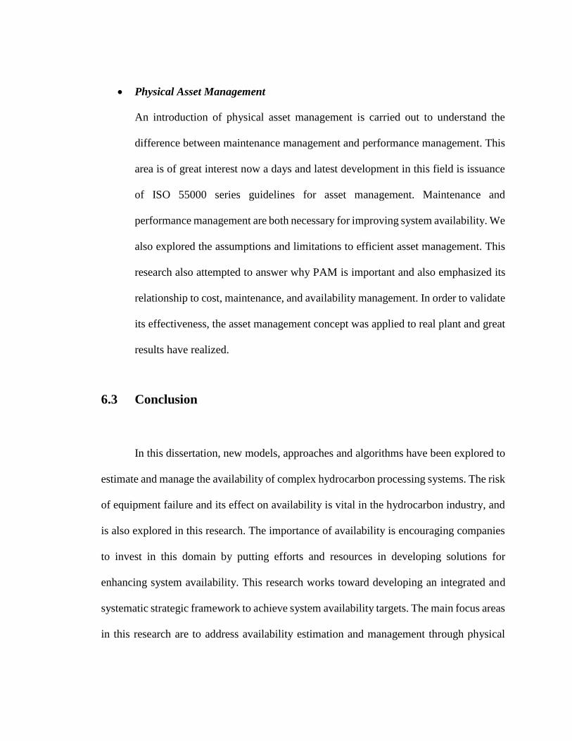
Physical Asset Management
An introduction of physical asset management is carried out to understand the
difference between maintenance management and performance management. This
area is of great interest now a days and latest development in this field is issuance
of ISO 55000 series guidelines for asset management. Maintenance and
performance management are both necessary for improving system availability. We
also explored the assumptions and limitations to efficient asset management. This
research also attempted to answer why PAM is important and also emphasized its
relationship to cost, maintenance, and availability management. In order to validate
its effectiveness, the asset management concept was applied to real plant and great
results have realized.
6.3 Conclusion
In this dissertation, new models, approaches and algorithms have been explored to
estimate and manage the availability of complex hydrocarbon processing systems. The risk
of equipment failure and its effect on availability is vital in the hydrocarbon industry, and
is also explored in this research. The importance of availability is encouraging companies
to invest in this domain by putting efforts and resources in developing solutions for
enhancing system availability. This research works toward developing an integrated and
systematic strategic framework to achieve system availability targets. The main focus areas
in this research are to address availability estimation and management through physical

asset management, risk-based availability estimation strategies, availability and safety
using a failure assessment framework, and availability enhancement using early equipment
fault detection and maintenance scheduling optimization.
In conclusion, this research will contribute to the field by providing a wide range
of solutions to industry in terms of availability estimation and management. The challenges
faced during the research, such as the availability and quality of the equipment historical
data, is dealt by normalizing the data with experience and recommendations from subject
matter experts. The algorithms, models, and solutions developed and presented in this
dissertation are valuable for estimating system availability and management. The proposed
solutions can assist strategic and tactile plant management in making decisions; and to
effectively and efficiently optimize system availability and cost.
6.4 Recommendations for Future Research Work
In this research, along with development of new methods, we have key findings to
enhance or extend the developed work. Some of them are discuss below:
1. A risk-based methodology of availability estimation is proposed. This
methodology assumed a constant failure rate, but work can be extended to develop state-
dependent models with different failure behaviors. The model can be extended to
equipment dominant failure modes. The flexibility of state-dependent models can be very

useful in these circumstances. Not only in regard to failure mode but also for other
constraints such as maintenance manpower, delays related to obtaining spare parts, and
equipment release for maintenance can be included to extend this work.
2. A risk-based failure assessment framework is explored for managing
availability and safety. This work can be extended to develop software tools which provide
users with a graphic user interface to follow the proposed framework. The proposed
framework has four key phases, which require multiple data handling and storage solutions.
A software tool developed based on the proposed framework greatly helps with
streamlining the process. It will also help with storing evidence, photos, and other
documents in a common database. Along with these benefits it will help with the tracking
and implementation of the recommendations.
3. Fault detection is an important aspect of availability enhancement. A
decision tree-based fault detection scheme is proposed in this dissertation, but there are
other algorithms available to detect incipient machinery faults. The work can be extended
to evaluate the performance of other algorithms and filtering techniques in detecting
machinery faults such as neural networks, Kalman filters, real coded genetic algorithms,
wavelet-based algorithms, and other hybrid algorithms. The suggested work extension will
explore the efficiency and suitability of decision trees and other algorithm responses to
detect incipient faults. The work can also be extended to explore other machinery failure
modes such as cracked shafts, rubbing, looseness, etc.
4. Maintenance optimization is an area of research for ensuring the safety,
reliability, and availability of equipment and systems. The exact and Pareto-optimal

solutions for multi-constrained maintenance scheduling optimization are discussed in this
dissertation. This work can be extended to optimize maintenance scheduling to include
other constraints such as maintenance manpower, equipment shutdown opportunity,
seasonal product demand changes, and spare availability. There are optimization
algorithms such as harmony, nature-inspired optimization, simulated annealing, and other
hybrid algorithms that can be explored further to develop maintenance schedules and
compare their optimization efficiency with proposed genetic algorithms.
REFERENCES
References - Chapter 1
[1] British Standard (BS EN 13303: 2001 E), Maintenance Terminology, British
Standard Institute
[2] Ebeling, C. E., (1996), An Introduction to Reliability and Maintainability
Engineering, 2nd edition, McGraw-Hill
[3] Gulati, R., Smith, R., (2009), Maintenance and Reliability Best Practices, 1st
Edition, Industrial Press, Inc.
[4] Military Standard MIL-STD-721C (1981), Definition of term from reliability and
maintainability.
[5] Bloch H., and Fred G., (1994), An introduction to machinery and reliability
assessment. Gulf Publishing company, 2nd edition, ISBN 0-88415-172-7
[6] Rausand, M., Hoyland A., (2004). System Reliability Theory Models, Statistical
Methods and Applications. John Wiley and Sons Inc., Norwegian University of
Science and Technology, 2nd edition, January, ISBN 0-471-47133-X
[7] Rujiroj L., April (2007), Availability Assessment of HVDC Converter
Transformers Using Markov Modeling, XR-EE-ETK 2007:002
[8] Hills, W. P., (2001), Plant Asset Management – PWH28 – CM2001 Oxford June
2001 (www.imamu.edu.sa)
[9] Physical Asset Management Program Brochure, University of Toronto, Canada
[10] Attou, A.K., and Ahmed, Q. (2009), Asset Management Practices at Qatargas,
Proceedings of the 1st Annual Gas Processing Symposium, Elsevier B.V.
[11] James W. Davis, PE, (2004), Creating a Reliability Culture in your Company”, The
Instrumentation Systems and Automation society, presented at the ISA-2004
[12] Kaplan, S., and Garrick, B.S., (1981), On the quantitative definition of risk, Risk
Analysis, Vol 1, pp 11-27
[13] Torhaug, M., (1990), Use of risk analysis in the offshore industry, Proceeding of
International Offshore Mechancis and Arctic Engineering Symposium, Vol. 2, pp
277-282
[14] Keshavarz, G., Thodi, P., Khan F., (2011), Risk-based shutdown management of
LNG units, Journal of Loss Prevention in the Process Industries, Vol. 25, pp 159-
166
[15] Freking, R.F., (1990), Availability model of a high-availability communication
network, Modeling and Simulation, Vol. 21, pp 813-825
[16] Maciejewski H., Caban D., (2008), Estimation of repairable system availability
within fixed time horizon. Reliability Engineering & System Safety, Vol. 93, pp.
100-106
[17] Mohanty, R. P., Singh, R., Availability Estimation for an Iron Ore Production Plant
Using Simulation, IJQRM, Vol 10
[18] Barabady, J., Kumar, U., (2008), Reliability analysis of mining equipment: A case
study of a crushing plant at Jajaram Bauxite mine in Iran. Reliability Engineering
& System Safety, Vol. 93, pp. 647-653

[19] Sonawane, B.U., Ahuja, B.B.,(2009),Modelling for availability of a reliability
based system using montecarlo simulation and markov chain analysis. Journal of
the Institution of Engineers (India), Vol. 90, pp. 36-40
[20] Smati, A., Younsi, K., Zeraibi, N., Zemmour, N.,(2003), LNG Chain availability
using Bayesian estimation of reliability rates. Oil and Gas Science and Technology,
Vol 58, pp 531-549
[21] Yoichi, W., (1987), Errors in Availability estimation by2-state models of 3-state
systems, Reliability Engineering, Vol 18, pp 223-235
[22] Mohanty, R.P., Mohanty, K.K., (1986), Availability estimation of a cement plant
through simulation, Maintenance Management International, Vol 6, pp 167-180
[23] Way, K., (1985), Bayesian Availability using Gamma distribution priors, IIE
Transactions, Vol 17, pp 132-140
[24] Cochran, J.K., Murugan, A., Krishnamurthy, V., (2000), Generic Markov models
for availability estimation and failure-characterization in petroleum refineries,
Computer and Operation Research, Vol. 28, pp 1-12
[25] Sherwin, D.J., (2000), Steady state series availability, IEEE Transaction on
Reliability, Vol 49, pp 131 – 132
[26] Zhao, M., (1994), Availability for repairable components and series systems, IEEE
Transaction on Reliability, Vol 43, pp 329 – 334
[27] Vidojevic, D., Jeremic, B., Babic, M., (2009), Availability management of complex
technical systems, Journal of Mechanical Engineering, Vol. 55

[28] Chae, H.S., Cui, J.F., Park, J.W., Park, J.G., Lee, W. J., (2009), An object-oriented
framework approach to flexible availability management for developing distributed
applications, Journal of Information Science and Engineering, Vol. 25, pp 1021-
1039
[29] Ola, K., (2004), Lifecycle management for improved product and system
availability, ABB Review, pp 36-37
[30] Lundteigen, M.A., Rausand, m., Utne, I.B., (2009), Integrating RAMS engineering
and management with safety life cycle of IEC 61508, Reliability Engineering and
System Safety, Vol. 94, pp 1894-1903
[31] Pil, C. K., Rausand, M., and Vatn, J., (2008), Reliability assessment of re-
liquefaction systems on LNG carriers, Reliability Engineering & System Safety,
Vol. 93, pp. 1345-1353
[32] Vesely E. Q., “(1977), Failure data and Risk Analysis, Proceedings of ‘The Energy
Technology Conference Houston, Texas’
References - Chapter 2
[1] Ebeling, C. E., (1996) “An Introduction to Reliability and Maintainability
Engineering”, 2nd Edition, McGraw-Hill
[2] Chang, D., Rhee, T., Nam, K.., Chang, K., Lee, D., & Jeong, S., (2008), “A study
on availability and safety of new propulsion systems for LNG carriers”, Reliability
Engineering & System Safety, Vol. 93, pp. 1877-1855

[3] Kales P., (1998) “Reliability for Technology, Engineering and Management’,
Prentice-Hall, Inc.
[4] Gulati, R., & Smith, R., (2009) “Maintenance and Reliability Best Practices”, 1st
Edition, Industrial Press, Inc.
[5] Khan, F. I., Haddara, M., & Krishnasamy, L., (2008) “A new methodology of risk-
based availability analysis”, IEEE Transactions on Reliability, Vol. 57, pp. 103-
112
[6] Sonawane, B.U., & Ahuja, B.B., (2009) “Modeling for availability of a reliability
based system using Monte Carlo simulation and Markov chain analysis”, Journal
of the Institution of Engineers (India), Vol. 90, pp. 36-40
[7] Pil, C. K., Rausand, M., & Vatn, J., (2008) “Reliability assessment of re-
liquefaction systems on LNG carriers”, Reliability Engineering & System Safety,
Vol. 93, pp. 1345-1353
[8] Keeter, B., (2003) “Using Reliability Engineering Methods as a Tool for
Continuous Process Improvement”, 18th International Maintenance Conference,
USA
[9] Jacob, D., & Amari, S., (2005) “Analysis of complex repairable systems”, Institute
of Electrical and Electronics Engineers, Vol. 54, pp. 517 - 529
[10] Moore R., (2003) “Making Common Sense Common Practices”, 3rd Edition,
Elsevier Butterworth-Heinemann
[11] Mobley, R., & Smith, R., (2008) “Rules of Thumb from Maintenance and
Reliability Engineers”, 1st Edition, Butterworth-Heinemann
[12] Ouhbi, B., & Limmios, N., (1997) “Reliability Estimation of semi-Markov system:
a case study” Reliability Engineering & System Safety, Vol. 58, pp. 201-204
[13] Cekyay B., & Ozekici, S. (2010) “Mean time to failure and availability of semi-
Markov missions with maximal repair”, European Journal of Operational Research,
Vol. 207, pp. 1442-1454
[14] Csenki, A., (1996) “A new approach to the cumulative operational time for semi-
Markov models of repairable systems”, Reliability Engineering & System Safety,
Vol. 54, pp. 11-21
[15] Smith, J. B., (2011) “Probabilistic availability risk assessments without
simulation”, Proceedings -Reliability and Maintainability Symposium, pp. 1-7
[16] Zhan, S., Grayson, B., (2012) “Optimal Reliability, Availability and Maintenance
(RAM) management for Oil Field Services”, IEEE Prognostics and System Health
Management, pp. 1-7
[17] Brok, J.F.C., (1987) "Availability Assessment of Oil and Gas Production Systems",
International Journal of Quality & Reliability Management, Vol. 4, pp.21 – 36
[18] Castro, H. F., Cavalca, K. L., (2003) "Availability optimization with genetic
algorithm", International Journal of Quality & Reliability Management, Vol. 20,
pp. 847 – 863
[19] Mokhatab, S., Poe, W.A., & Speight, J. G., (2006) “Handbook of Natural Gas
Transmission and Processing”, Gulf Professional Publishing
[20] Modarres, M., (2006) “Risk Analysis in Engineering – Techniques, Tools and
Trends” CRC Press

[21] Crowl, D. A., & Louvar, F. J., (2001) “Chemical Process safety, Fundamental with
application”, 2nd Edition , Prentice-Hall, Inc.
[22] OREDA., (2002) “Offshore Reliability Data Handbook” 4th Edition
References - Chapter 3
[1] Bloch, K., Bertsch, J., Dunmire, D., (2011), “Update your reliability performance
to meet process safety expectations”, published in Hydrocarbon Processing,
presented in 7th Global Congress on Process Safety, Illinois, USA.
[2] Bloch, Heinz P.; Geitner, Fred K. (2012). Machinery Failure Analysis and
Troubleshooting, Volume 2 - Practical Machinery Management for Process Plants
(4th Edition), Elsevier.
[3] ISO 10303:1994 - Industrial Automation Systems and Integration - Product Data
Representation and Exchange.
[4] Define: Fault (technology), http://en.wikipedia.org/wiki/Fault_(technology),
accessed on 7th July 2013
[5] C. Ebeling, (2001) “An Introduction to Reliability and Maintainability
Engineering”, Tata McGraw-Hill, New York, NY, USA,
[6] Márquez, A. C., (2007),”The Maintenance Management Framework: Models and
Methods for Complex Systems Maintenance”, Springer Series in Reliability
Engineering, London, United Kingdom
[7] Bhote, K. R. (1988), “World class quality: Design of experiments made easier,
more cost effective than SPC”. New York: AMA.
[8] Doggett A. M., (2005), “Root Cause Analysis: A Framework for Tool Selection”,
ASQ – Quality Management Journal, Vol. 12
[9] R J Latino and K C Latino, (1999), “Root Cause Analysis – Improving Performance
for Bottom Line Results”, CRC Press, pp 87-88
[10] A. Adamyan and D. He, (2002) “Analysis of sequential failures for assessment of
reliability and safety of manufacturing systems,” Reliability Engineering and
System Safety, vol. 76, pp.227–236.
[11] A. Adamyan and D.He, (2004) “System failure analysis through counters of Petri
net models,” Quality and Reliability Engineering International, vol. 20, pp. 317–
335.
[12] Andrews J.D., Dugan J.B., (1999), “Dependency Modeling using Fault Tree
Analysis”, 17th International Safety System Conference, available at
http://www.fault-tree.net
[13] Houtermans, M., Al-Ghumgham, M., Capelle, T.V., (2008),"Improve industrial
process plant safety & availability via reliability engineering," Computer Systems
and Applications, IEEE/ACS International Conference, Doha, Qatar,
pp.1021,1026.
[14] Baraldi, P., Mangili, F. and Zio, E., (2012) “A Kalman Filter-Based Ensemble
Approach With Application to Turbine Creep Prognostics” IEEE Transactions on
Reliability, Vol. 61, pp. 966-977
[15] Chen Z. S., Yang Y. M. and Hu Z., (2012), “A Technical Framework and Roadmap
of Embedded Diagnostics and Prognostics for Complex Mechanical Systems in
Prognostics and Health Management Systems”, IEEE Transactions on Reliability,
Vol. 61, pp. 314-322
[16] Ma, S. Z. and Krings, W. A., (2011), ”Dynamic Hybrid Fault Modeling and
Extended Evolutionary Game Theory for Reliability, Survivability and Fault
Tolerance Analyses”, IEEE Transactions on Reliability, Vol. 60, pp. 180-196
[17] Khan, F. I., Haddara, M., and Krishnasamy, L., (2008) “A New Methodology for
Risk-Based Availability Analysis”, IEEE Transactions on Reliability, Vol. 57, pp.
103-112
[18] Cassady, C. R., Iyoob, M. I., Schneider, K. and Pohl A. E., “A Generic Model of
Equipment Availability Under Imperfect Maintenance”, IEEE Transactions on
Reliability, Vol. 54, 2005, pp. 564-571
[19] Varvarigou, A. T. and Ahuja, S. C., (1997) “ MOFA: A Model for Fault &
Availability in Complex Services”, IEEE Transactions on Reliability, Vol. 46, pp.
222-232
[20] Campbell D. J., Jardine K. S. A., (2001), “Maintenance Excellence: Optimizing
Equipment Life-Cycle Decisions”, Marcel Dekker, Inc.
[21] Attou, A.K., and Ahmed, Q., (2009), “Asset Management Practices at Qatargas”,
Proceedings of the 1st Annual Gas Processing Symposium, Qatar, Doha, Elsevier
B.V., pp. 286-296
[22] Ahmed. Q., (2011), “RCFA Case Study: Infant Mortality: Lean Solvent Centrifugal
Pump Motor”, The 1st Texas A&M Middle East Turbo-machinery Symposium
(METS), Doha, Qatar
[23] Kales, P., (1998), “Reliability: For Technology, Engineering, and Management”,
Prentice Hall, USA
References - Chapter 4
[1] Andrews, J.D. and Moss, T.R., (1993), “Reliability and Risk Assessment,”
Published by Longman Scientific & Technical, U.K. and John Wiley & Sons Inc.,
USA. First Edition, pp. 152.
[2] Smith, J.S., (1997), “Reliability, Maintainability and Risk,” Published by
Butterworth-Heinemann. Fifth Edition, pp. 9.
[3] Gulati, R., (2012), Maintenance and Reliability Best Practices by Ramesh Gulati
Published by Industrial Press; Second Edition.
[4] Rotating Unbalance, http://en.wikipedia.org/wiki/Rotating_unbalance, accessed on
July 8, 2014.
[5] Precision Maintenance Techniques for Machinery, Machine Installation – Shaft
Alignment, accessed on July 8, 2014, http://www.lifetime-reliability.com/tutorials.
[6] B. Peter, “Using vibration analysis for machinery fault diagnostics,” Article from
www.lifetime-reliability.com accessed on May 1, 2014.
[26] Fathima, A.S., Manimegalai, D. and Hundewale N., (2011), “A Review of Data
Mining Classification Techniques Applied for Diagnosis and Prognosis of the
Arbovirus-Dengue,” IJCSI International Journal of Computer Science Issues, Vol.
8, pp. 322-328.

[8] Brambilla, D., Capisani, L.M., Ferrara, A. and Pisu, P., (2008), “Fault detection for
robot manipulators via second-order sliding modes.” IEEE Trans. Ind. Electron.
Vol. 55, pp 3954-3963.
[9] Cusido J., Romeral, L., Ortega, J.A., Rosero, J.A., Garcia, A.E., (2008), “Fault
detection in induction machines using power spectral density in wavelet
decomposition,” IEEE Trans. Ind. Electron., Vol. 55, pp. 633-643.
[10] Arogeti, S.A., Wang, D., Low, C.B., (2010), “Mode Identification of Hybrid
Systems in the Presence of Fault.” IEEE Trans. Ind. Electron. Vol. 57, pp. 1452-
1467.
[11] Lezana, P., Pou, J., Meynard, T.A., Rodriguez, J., Ceballos, S. and Richardeau, F.
(2010), “Survey on Fault Operation on Multilevel Inverters.” IEEE Trans. Ind.
Electron. Vol. 57, pp. 2207-2218.
[12] Morgan, I., Liu, H., Tormos B. and Sala A., (2010), “Detection and diagnosis of
incipient faults in heavy-duty diesel engines.” IEEE Trans. Ind. Electron. Vol. 57,
pp. 3522-3532.
[13] Poncelas, O., Rosero, J.A., Cusido, J., Ortega J.A. and Romeral L., (2009), “Motor
fault detection using a rogowski sensor without an integra.” IEEE Trans. on Ind.
Electron. Vol. 56, pp. 4062-4070.
[14] Rothenhagen, K. and Fuchs, F.W., (2009), “Current sensor fault detection,
isolation, and reconfiguration for doubly fed induction generator.” IEEE Trans. on
Ind. Electron. Vol. 56, pp. 4239-4245.

[15] Saimurugan, M., Ramachandran, I.K., Sugumaran, V., Sakthivel, R.N., (2011),
“Multi component fault diagnosis of rotational mechanical system based on
decision tree and support vector machine,” Expert Systems with Applications, Vol.
38, pp. 3819-3826.
[16] Amarnath, M., Sugumaran, V., Kumar, H., (2013), “Exploiting sound signals for
fault diagnosis of bearings using decision tree,” Journal of Measurement, Vol. 46,
pp. 1250-1256.
[17] Tran, V.T., Yang, B. and Oh, Myung-S., (2006) “Fault Diagnosis of Induction
Motors using Decision Trees.” KSNVE Annual Autumn Conference, Tongyoung,
Korea.
[18] Ma, S.Z. and Krings, W.A., (2011),”Dynamic Hybrid Fault Modeling and Extended
Evolutionary Game Theory for Reliability, Survivability and Fault Tolerance
Analyses,” IEEE Transactions on Reliability, Vol. 60, pp. 180-196.
[19] Khan, F.I., Haddara, M. and Krishnasamy, L., (2008), “A New Methodology for
Risk-Based Availability Analysis,” IEEE Transactions on Reliability, Vol. 57, pp.
103-112.
[20] Yang, B.S., Park, H.C. and Kim, J.H., (2000) “An Efficient Method of Vibration
Diagnostics for Rotating Machinery using a Decision Tree,” International Journal
of Rotating Machinery, Vol. 6, pp. 19-27.
[21] Sugumaran, V., Jain, D., Amaranath, M. and Kumar, H., (2013), “Fault Diagnosis
of Helical Gear Box using Decision Tree through Vibration Signals,” International
Journal of Performability Engineering, Vol. 9, No. 2, pp.221-233.

[22] Sugumaran, V. and Ramachandran, K.I., (2007), “Automatic rule learning using
decision tree for fuzzy classifier in fault diagnosis of roller bearing,” Mechanical
Systems and Signal Processing, Vol. 21, Issue 5, pp. 2237-2247.
[23] Sun, W., Chen, J., Li, J., (2007), “Decision tree and PCA-based fault diagnosis of
rotating machinery,” Mechanical Systems and Signal Processing, Vol. 21, Issue 3,
April 2007, pages 1300-1317.
[24] Boumahdi, M., Dron, P.J., Rechak, S. and Cousinard, O., (2010), “On the
extraction of rules in the identification of bearing defects in rotating machinery
using decision tree,” Expert Systems with Applications, Vol. 37, Issue 8, pp. 5887-
5894.
[25] Ngoc-Tu, N., Jeong-Min, K. and Hong-Hee L., (2007), “A Study on Machine Fault
Diagnosis using Decision Tree,” Journal of Electrical Engineering & Technology,
Vol. 2, pp. 461-467.
[26] MATLAB “Help” on Optimization Criterion: website accessed on May 6. 2014.
http://www.mathworks.com/help/stats/classificationtree-class.html
[27] Robichaud, M.J., “Report on Vibration limits Reference Standards for Vibration
Monitoring and Analysis,” accessed on May 15, 2014. http://www.bretech.com/.
[28] Equipment Datasheet - RK4 Rotor kit, Bentley Nevada TM Asset Condition
Monitoring.
References - Chapter 5

[1] Wireman, T., (2007), “Preventive Maintenance (Maintenance Strategy Series),
Publisher: Industrial Press, Inc. NY, USA
[2] Gulati, R., Smith, R., (2009), “Maintenance and reliability best practices”. :
Publisher: Industrial Press, Inc. NY, USA
[3] http://en.wikipedia.org/wiki/Predictive_maintenance, accessed on 26th May 2014
[4] Ahmed, Q., Khan, I. F., Raza, A. S., (2014) "A risk-based availability estimation
using Markov method", International Journal of Quality & Reliability
Management, Vol. 31 , pp. 106 – 128.
[5] Moghaddam, S. K., Usher, S. J., (2011), “Preventive maintenance and replacement
scheduling for repairable and maintainable systems using dynamic programming”,
Computers & Industrial Engineering, Vol. 60, pp. 654-665.
[6] Dopazo, J.F., Merrill, H.M., (1975) "Optimal generator maintenance scheduling
using integer programming," Power Apparatus and Systems, IEEE Transactions on
, vol.94, pp. 1537-1545.
[7] Tsai, T. Y., Wang, S. K., Teng, Y. H., (2001), “Optimizing preventive maintenance
for mechanical components using genetic algorithms, Reliability Engineering &
System Safety, Vol. 74, pp. 89-97.
[8] Painton, L.; Campbell, J., (1995), "Genetic algorithms in optimization of system
reliability," Reliability, IEEE Transactions on , Vol. 44, pp. 172-178.
[9] Coit, D.W.; Smith, A.E., (1996), "Reliability optimization of series-parallel
systems using a genetic algorithm," Reliability, IEEE Transactions on , vol.45, pp.
254-266.

[10] Gen, M., Cheng. R., (2000), “Genetic Algorithms and Engineering Optimization”,
John Wiley and Sons.
[11] Hadi, M., , Ashkan, M., & Isa, N. K. A., (2012), “A reliability/availability approach
to joint production and maintenance scheduling with multiple preventive
maintenance services”, International Journal of Production Research, Vol. 50, pp.
5906-5925.
[12] Chen, S. K., Wang, X. D., Bai, Y., Liu, H. D., Mao, B. H., (2013), “Lowest costs-
based optimum maintenance scheduling model for catenaries of railways”, Journal
of the China Railway Society, Vol. 35, pp 37-42.
[13] Suresh, K., Kumarappan, N., (2013) “Hybrid improved binary particle swarm
optimization approach for generation maintenance scheduling problem, Swarm and
Evolutionary Computation”, Vol. 9, pp 69-89
[14] El-Sharkh, M. Y., (2014), “Clonal selection algorithm for power generators
maintenance scheduling”, International Journal of Electrical Power & Energy
Systems, Vol 57, pp. 73-78.
[15] Vatn J., Hokstad P., Bodsberg L., (1996), “An overall model for maintenance
optimization. Reliability Engineering and System Safety, Vol. 51, pp. 241–257.
[16] Clarotti C. A., Lannoy A., Procaccia H., (1997) “Probabilistic risk analysis of
ageing components which fail on demand; a Bayesian model: application to
maintenance optimization of diesel engine linings”. Proceedings of Ageing of
Materials and Methods for the Assessment of Lifetimes of Engineering Plant, Cape
Town, pp. 85–94.
[17] Khan, F. I. and Haddara, M. (2004), Risk-based maintenance (RBM): A new
approach for process plant inspection and maintenance. Proc. Safety Prog., Vol. 23,
pp. 252–265.
[18] Xu, B., Han, X., Wang, Y., Sun, D., (2012), “ Risk-based optimization model for
system maintenance scheduling”, 2012 IEEE International Conference on Power
System Technology, Auckland, New Zealand.
[19] Schlünz, E.B., Van V. J. H., (2013), “An investigation into the effectiveness of
simulated annealing as a solution approach for the generator maintenance
scheduling problem, International Journal of Electrical Power and Energy Systems,
Vol. 53, pp. 166-174.
[20] Gustavsson, E., Patriksson, M., Stromberg, A. B., Wojciechowski, A., Onnheim,
M., (2014), “Preventive maintenance scheduling of multi-component systems with
interval costs”, Computers and Industrial Engineering, Article in Press.
[21] Reihani, E., Sarikhani, A., Davodi, M., Davodi, M., (2012), “Reliability based
generator maintenance scheduling using hybrid evolutionary approach”,
International Journal of Electrical Power & Energy Systems, Vol. 42, pp. 434-439.
[22] Aghaie, M., Norouzi, A., Zolfaghari, A., Minuchehr, A., Mohamadi F. Z., Tumari,
R., (2013), “Advanced progressive real coded genetic algorithm for nuclear system
availability optimization through preventive maintenance scheduling”, Annals of
Nuclear Energy, Vol. 60, pp. 64-72.
[23] Giftson S. G., Christober A. R. C., (2012) “A modified genetic approach to long-
term generation maintenance scheduling to enhance the reliability of the units”,

Proceeding of IEEE-International Conference on Advances in Engineering,
Science and Management, pp. 789-793.
[24] Fu, F., (2013), “Maintenance scheduling optimization for electromechanical
equipment based on reliability” Computer Integrated Manufacturing Systems”,
Vol. 19, pp. 2940-2946
[25] Ajit K. V., Srividya, A., Rana, A., Sanjay K. K., (2012), “Optimization of
maintenance scheduling of ship borne machinery for improved reliability and
reduced cost”, International Journal of Reliability, Quality and Safety Engineering,
Vol. 19
[26] Ahmadi, R., Newby, M., (2011), “Maintenance scheduling of a manufacturing
system subject to deterioration”, Reliability Engineering & System Safety, Vol 96,
pp. 1411-1420.
[27] Berrade, M.D., Cavalcante, A. V. C., Scarf, A. P., (2012), “Maintenance
scheduling of a protection system subject to imperfect inspection and replacement”,
European Journal of Operational Research, Vol. 218, pp. 716-725.
[28] Rahimdel, J. M., Ataei, M., Khalokakaei, R., Hoseinie, H. S., (2013), “Reliability-
based maintenance scheduling of hydraulic system of rotary drilling machines”,
International Journal of Mining Science and Technology, Vol. 23, pp. 771-775.
[29] Go, H., Kim, J. S., Lee, D., (2013), “Operation and preventive maintenance
scheduling for containerships: Mathematical model and solution algorithm,
European Journal of Operational Research, Vol. 229, pp. 626-636.
[30] Lapa F. M. C., Pereira, M. C., Barros, P. M., (2006), “A model for preventive
maintenance planning by genetic algorithms based in cost and reliability”,
Reliability Engineering & System Safety, Vol. 91, pp. 233-240.
[31] Samrout, M., Yalaoui, F., Châtelet, E., Chebbo, N., (2005), “New methods to
minimize the preventive maintenance cost of series–parallel systems using ant
colony optimization”, Reliability Engineering & System Safety, Volume 89, pp.
346-354.
[32] Konak, A., Coit, W. D., Smith, E. A., (2006), “Multi-objective optimization using
genetic algorithms: A tutorial”, Reliability Engineering & System Safety, Volume
91, pp. 992-1007.
[33] Certa, A., Galante, G., Lupo, T., Passannanti, G., (2011), “Determination of Pareto
frontier in multi-objective maintenance optimization”, Reliability Engineering &
System Safety, Volume 96, pp. 861-867.
[34] Bertolini, M., Bevilacqua, M., (2006), “A combined goal programming—AHP
approach to maintenance selection problem”, Reliability Engineering & System
Safety, Vol. 91, pp. 839-848.
[35] Moghaddam S. K., (2013), “Multi-objective preventive maintenance and
replacement scheduling in a manufacturing system using goal programming”,
International Journal of Production Economics, Vol. 146, pp 704-716.
[36] LINGO website: http://www.lindo.com / An Overview of LINGO, accessed on 16th
December 2014.

References - Chapter 6
[1] Reliability, An IEEE Spectrum Compendium, October 2001, USA