Embed Size (px)
Citation preview

Autovetter Planet Candidate Catalog
for Q1-Q17 Data Release 24
KSCI-19091-001
Joseph H. Catanzarite
20 July 2015
NASA Ames Research Center
Moffett Field, CA 94035

KSCI-19091-001: Autovetter Planet Candidate Catalog 7/20/15
1
Prepared by: _________________________________________ Date 7/20/15
Joseph H. Catanzarite, Scientific Programmer
Approved by: ________________________________________ Date 7/20/15
Jon M. Jenkins, Mission Analysis Lead
Approved by: ________________________________________ Date 7/20/15
Natalie M. Batalha, Mission Scientist
Approved by: ________________________________________ Date 7/20/15
Michael R. Haas, Science Office Director
Approved by: ________________________________________ Date 7/20/15
Steve B. Howell, Project Scientist

KSCI-19091-001: Autovetter Planet Candidate Catalog 7/20/15
2
Document Control
Ownership
This document is part of the Kepler Project Documentation that is controlled by the
Kepler Project Office, NASA/Ames Research Center, Moffett Field, California.
Control Level
This document will be controlled under KPO @ Ames Configuration Management
system. Changes to this document shall be controlled.
Physical Location
The physical location of this document will be in the KPO @ Ames Data Center.
Distribution Requests
To be placed on the distribution list for additional revisions of this document, please
address your request to the Kepler Science Office:
Michael R. Haas
Kepler Science Office Director
MS 244-30
NASA Ames Research Center
Moffett Field, CA 94035-1000
or

KSCI-19091-001: Autovetter Planet Candidate Catalog 7/20/15
3
DOCUMENT CHANGE LOG
CHANGE DATE PAGES
AFFECTED CHANGES/NOTES
July 20, 2015 all First issue

KSCI-19091-001: Autovetter Planet Candidate Catalog 7/20/15
4
Table of Contents
1. Introduction............................................................................................................. 5
2. Autovetter Inputs..................................................................................................... 7
3. Autovetter Outputs................................................................................................. 8
4. Decision Trees and the Random Forest.................................................................. 9
5. The Attributes Matrix............................................................................................ 10
6. Building the Training Set...................................................................................... 14
7. Posterior Class Probabilities ................................................................................. 18
8. Autovetter Results for the Q1-Q17 DR24 TCEs................................................... 20
9. References..............................................................................................................33

KSCI-19091-001: Autovetter Planet Candidate Catalog 07/16/2015
5
1. Introduction
The autovetter is a machine learning based classifier that dispositions TCEs into three
classes: PC (Planet Candidate), AFP (Astrophysical False Positive), and NTP (Non-
Transiting Phenomenon), defined as follows:
Class PC contains signals that are consistent with transiting planets, and for which no
known reason exists to rule out that hypothesis.
Class AFP contains signals of astrophysical origin that could mimic planetary transits,
such as detached and contact eclipsing binaries, pulsating stars, starspots, and other
periodic signals for which there is strong evidence to rule out a transiting planet
origin.
Class NTP contains signals that are evidently of instrumental origin, or are noise
artifacts.
This document describes the autovetter, and how it is used to produce a catalog of Planet
Candidates from the Q1-Q17 DR24 TCEs (Threshold Crossing Events) that are identified
in the Kepler SOC (Science Operations Center) pipeline [Jenkins 2010ab] version 9.2
[Seader et al. 2015].
Classification is accomplished by means of a decision tree-based machine learning
technique known as the random forest. The inputs to the autovetter are a training data
set composed of TCEs that have been dispositioned (mostly) by humans into these three
classes, and a set of attributes (scalar statistics) associated with each TCE. From the
training set, the autovetter ‘learns’ a mapping between attributes and predicted class. This
mapping is then applied uniformly and consistently to all TCEs to produce a catalog of
planet candidates.
1.1 Motivation for Another Planet Candidate Catalog
The Kepler project has produced the Q1-Q17 DR24 KOI (Kepler Object of Interest)
activity table, which is hosted by NExScI (NASA Exoplanet Science Institute) and
contains a catalog of planet candidates. This table was produced by the robovetter, an
expert system designed to automatically classify TCEs [Coughlin 2015], and will
henceforth be referred to as the robovetter catalog.
The autovetter produces a different catalog of planet candidates. One might ask: why
offer two catalogs? The autovetter and robovetter followed independent methodology to
arrive at the same goal – automation of the process of human classification of planet
candidates to achieve fast, robust and consistent vetting of the entire population of TCEs.
The ‘machine learning’ approach differs from the ‘expert system’ approach in that the
autovetter’s decision rules are ‘learned’ autonomously from the data, while the robovetter
operates with explicitly constructed decision rules.
The autovetter and robovetter evolved in parallel, learning from each other iteratively.
The process has benefitted both, improving their respective planet catalogs. For example,
early robovetter results indicated that the autovetter was initially misclassifying some
TCEs with secondary eclipses as planet candidates; by adding new attributes we

KSCI-19091-001: Autovetter Planet Candidate Catalog 7/20/15
6
improved the autovetter’s ability to correctly classify secondary eclipses. In the other
direction, autovetter results showed that the robovetter was too strongly rejecting
candidates based on diagnostics indicating a possible centroid offset, which allowed the
robovetter to be tuned to mitigate that problem.
Though the two catalogs have converged over time, they don’t always agree on
classification for individual TCEs, nor would we expect them to, given the distinctly
different origin of the decision rules for the autovetter and robovetter. As an example the
autovetter tends to classify planets that are large enough and bright enough to have
secondary eclipses as AFPs, while the robovetter is tuned to be able to identify them as
PCs.
Another important difference is that while the autovetter has three classifications,
PC/AFP/NTP, the robovetter has four flags: Not Transit-Like, Significant Secondary,
Centroid Offset, and Ephemeris Match. These flags allow various sub-populations (e.g.,
on- and off-target EBs, off-target flux PCs, secondary eclipses) to be selected for further
study.
The most important difference between the catalogs is that in addition to a predicted
classification for each TCE, the autovetter also provides a Bayesian estimate of the
posterior probability that the TCE is a member of each class. For a given TCE, the
posterior probability for the class PC is a measure of the confidence that the TCE is a
planet. Posterior probabilities can be advantageously used in statistical studies such as
occurrence rate calculations to de-weight planet candidates that are at the noisy edges of
the planet catalog.
Finally, we note that the autovetter results, which can be found in the Q1-Q17 DR24 TCE
table at NExScI, change neither the dispositions in any KOI activity table nor the Kepler
planet candidate count.
1.2 Overview of This Document
We describe the autovetter inputs and outputs in sections 2 and 3. In section 4, we
provide some background on decision trees and the random forest. In section 5 we
describe the attributes that are used by the random forest to classify TCEs. In section 6,
we describe how the training set is constructed. In section 7 we describe the computation
and use of posterior class probabilities. In Section 8 we present the autovetter catalog and
give a detailed comparison of its results with those of the robovetter catalog. References
are provided in Section 9.

KSCI-19091-001: Autovetter Planet Candidate Catalog 7/20/15
7
2. Autovetter Inputs
The autovetter requires two inputs: the attributes matrix and the training data set.
Attributes are the scalar parameters and diagnostic statistics that are computed for each
TCE. They include fitted transit parameters (such as period, transit depth, transit epoch),
stellar parameters (such as effective temperature and gravity), as well as signal to noise
and chi-squared from the transit model fits. The attributes matrix has a row for each TCE
and a column for each attribute. A list of attribute names is provided in section 5.
The training data set consists of labels PC (planet candidate), AFP (astrophysical false
positive), and NTP (non-transiting phenomenon) for a subset of several thousand TCEs.
The PC labels in our training set are derived from dispositions originally produced via a
manual vetting process developed by the TCERT (Threshold Crossing Event Review
Team). The AFP and NTP labels come from TCERT dispositions combined with other
diagnostics. For the purpose of training the autovetter, the training set labels are
considered to be ‘ground truth’. The construction of the training data set is discussed in
detail in section 7.

KSCI-19091-001: Autovetter Planet Candidate Catalog 7/20/15
8
3. Autovetter Outputs
The autovetter produces the following outputs for each TCE:
a) Random forest vote fraction, in percent, for each class (PC, AFP, NTP),
b) Uncertainty in random forest vote fraction, in percent, for each class,
c) Posterior class probabilities that the TCE is a member of each of the three classes,
d) An autovetter-determined classification (PC, AFP or NTP), and
e) A training label (PC, AFP, or NTP), if the TCE was in the training set.
Description of the autovetter outputs
av_vf_pc, av_vf_afp, av_vf_ntp (float)
Vote fraction value for classes PC, AFP and NTP, respectively (float, in percent). For
each class, the vote fraction value is the mean class vote fraction for a set of 10 random
forest runs.
av_vf_pc_err, av_vf_afp_err, av_vf_ntp_err (float)
Uncertainty in the vote fraction for classes PC, AFP and NTP, respectively (float, in
percent). For each class, the error in the mean class vote fraction from a set of 10 random
forest runs is the standard deviation in the class vote fraction divided by the square root
of 10.
av_pp_pc, av_pp_afp, av_pp_ntp (float)
Posterior class probabilities for PC, AFP and NTP classifications, respectively (float, in
percent).
av_pred_class (char)
Classifications predicted by the autovetter, which are the optimum MAP (maximum a
posteriori) classifications. Values are ‘PC’, ‘AFP’, or ‘NTP’.
av_training_set (char)
Training labels: if the TCE was included in the training set, the training label encodes
what we believe is the ‘true’ classification, and takes a value of either ‘PC’, ‘AFP’, or
‘NTP’. Training labels are given a value of ‘UNK’ for TCEs that are not included in the
training set.
For details about the determination of posterior probabilities and optimum MAP
classifications see [Jenkins 2015c].

KSCI-19091-001: Autovetter Planet Candidate Catalog 7/20/15
9
4. Decision Trees and the Random Forest
A decision tree is a hierarchical series of one-dimensional inequalities that partitions the
phase space of attributes. At each split, a hyperplane divides a single attribute into a left
branch and a right branch, in which the attribute’s value is less than (left branch) or
greater than (right branch) the value at the split.
A split reduces entropy when it partitions the data into regions in which the class
populations are more sharply differentiated than they were before the split. Which
attribute to split on and the value of that attribute at the split are chosen to maximize the
resulting entropy reduction. Successive splits are carried out according to this entropy-
reduction principle. Each split produces two new branches in the tree. Splitting continues
until no further entropy-reducing splits are available. The terminal split on each branch
produces a pair of leaf nodes, regions of phase space in which the class populations
should be highly differentiated to favor one class. The full set of splits defines the
decision tree classifier, which maps any vector in attributes phase space to the predicted
classification associated with the leaf node in which the vector lies.
The random forest refines the decision tree approach in two ways. The first refinement is
called bootstrap aggregation or bagging. Instead of a single tree, a ‘forest’ of trees is
generated from a set of bootstrap samples of the training data set (also called a bag). A
bootstrap sample is an ensemble of examples drawn with replacement from the training
set, and of the same size as the training set. On average, a bootstrap sample uses about
2/3 of the training set. The remaining 1/3 of the training set are called out-of-bag
samples. Because they are not used in that decision tree, they are available to estimate
classification error without committing the crime of ‘data snooping’. For this reason, the
random forest does not require cross-validation to estimate classification error. Bagging
decreases the variance of the classifier, meaning that it reduces its sensitivity to the
characteristics of a particular training set, thus mitigating the problem of overfitting. The
second refinement is that at every split, the attribute to split on is chosen from a different
small random subset of the attributes, instead of from the entire set of attributes. If the
splitting attribute were always selected from the entire set of attributes, the trees will tend
to look similar, since the strongest attribute will be chosen at each split. Choosing the
splits from small random samples of attributes effectively decorrelates the trees. For
each example, the predicted class is then decided by the majority vote among all the trees
in the random forest.
The two parameters that control the random forest are the number of trees in the forest
and the size of the random subset of attributes to choose from at each split. The number
of trees can be optimized by incrementally increasing it until there is no improvement in
the classification error. We find that good results can be obtained with forests of 10,000
trees. Following standard practice, we took the size of the random subset of attributes that
is used at each split to be the square root of the number of attributes.
For more details about the random forest, see [Breiman 2001] and [James 2013].
Implementation of the random forest in the autovetter is discussed in [McCauliff 2015]
and [Jenkins 2015c].

KSCI-19091-001: Autovetter Planet Candidate Catalog 7/20/15
10
5. The Attributes Matrix
Attributes are scalar quantities that are computed for each TCE. Ideally, attributes capture
characteristics that aid in classification. Unlike classification methods that depend upon
distances between points in attribute phase space, the random forest is robust to missing
attribute values; not all attributes need exist for each example. Because each split must be
chosen from a small random subset of the attributes, the random forest is relatively robust
to correlations in the attributes.
An attribute’s importance is measured by the increase in the overall classification error
rate that would result from randomly scrambling the values of that attribute among all the
out-of-bag examples. Table 1 lists 114 attributes that the autovetter used, sorted in order
of importance. Attributes whose importance fell below an empirically determined
importance threshold of 5x10⁻⁵
were not used and are not listed. Sorted importances for
the 114 attributes are plotted in Figure 1.
Figure 1. Sorted importances for the 114 attributes used by the autovetter.
It is beyond the scope of this document to provide complete descriptions of all the
attributes in Table 1. That said, many of the attribute names are self-descriptive. Most of
the attributes are computed in the DV (Data Validation) section of the Kepler SOC
pipeline [Wu 2010]. It is possible, however, to formulate and compute new attributes post

KSCI-19091-001: Autovetter Planet Candidate Catalog 7/20/15
11
hoc, after the pipeline has completed. We have done this in several cases, which we will
discuss in the next section, where we will identify and describe a few of the most
important attributes and indicate how they are computed. For brief descriptions of more
of the important attributes, see [Jenkins 2015c].
Table 1. Attributes Used by the Autovetter and Their Importances 1. minLongerShorterPeriodSignificance
2. lppStatistic
3. numberOfPlanets
4. planetCandidate.weakSecondaryStruct.maxMes
5. planetCandidate.weakSecondaryStruct.mesMad
6. binaryDiscriminationResults.longerPeriodComparisonStatistic.significance
7. binaryDiscriminationResults.shorterPeriodComparisonStatistic.significance
8. binaryDiscriminationResults.longerPeriodComparisonStatistic.value
9. binaryDiscriminationResults.shorterPeriodComparisonStatistic.value
10. chiSquareGof
11. bootstrap_falseAlarmRate
12. evenTransitsFit_ratioSemiMajorAxisToStarRadius_value
13. oddTransitsFit_ratioSemiMajorAxisToStarRadius_value
14. maxEphemerisCorrelationAllStars
15. minMesMaxMesRatio
16. centroidResults.differenceImageMotionResults.mqKicCentroidOffsets.meanSkyOffset.value
17. edgeStat
18. allTransitsFit_ratioSemiMajorAxisToStarRadius_value
19. centroidResults.differenceImageMotionResults.mqKicCentroidOffsets.meanSkyOffset.significance
20. sesProbability
21. tEquilibrium
22. tBrightness
23. centroidResults.fluxWeightedMotionResults.motionDetectionStatistic.significance
24. allTransitsFit.modelFitSnr
25. allTransitsFit.modelChiSquare
26. centroidResults.fluxWeightedMotionResults.motionDetectionStatistic.value
27. allTransitsFit_orbitalPeriodDays_value
28. planetCandidate.modelChiSquare2
29. numSesInMes
30. evenTransitsFit_orbitalPeriodDays_value
31. centroidResults.differenceImageMotionResults.summaryQualityMetric.fractionOfGoodMetrics
32. oddTransitsFit_ratioSemiMajorAxisToStarRadius_uncertainty
33. evenTransitsFit_ratioSemiMajorAxisToStarRadius_uncertainty
34. evenTransitsFit.modelChiSquare
35. evenTransitsFit.modelFitSnr
36. modelFitSnrToMesRatio
37. centroidResults.differenceImageMotionResults.mqControlCentroidOffsets.meanSkyOffset.value
38. allTransitsFit_planetRadiusEarthRadii_value
39. centroidResults.fluxWeightedMotionResults.sourceOffsetArcSec.value
40. allTransitsFit_ratioSemiMajorAxisToStarRadius_uncertainty
41. effectiveTemp.value
42. centroidResults.differenceImageMotionResults.mqKicCentroidOffsets.meanSkyOffset.uncertainty
43. oddTransitsFit.modelChiSquare.reducedchi
44. oddTransitsFit_planetRadiusEarthRadii_value
45. evenTransitsFit_semiMajorAxisAu_value
46. centroidResults.differenceImageMotionResults.mqControlCentroidOffsets.meanSkyOffset.uncertainty
47. chiSquare7
48. evenTransitsFit_planetRadiusEarthRadii_value
49. allTransitsFit_semiMajorAxisAu_uncertainty

KSCI-19091-001: Autovetter Planet Candidate Catalog 7/20/15
12
50. chiSquare1
51. allTransitsFit_ratioPlanetRadiusToStarRadius_value
52. oddTransitsFit_ratioPlanetRadiusToStarRadius_value
53. allTransitsFit_orbitalPeriodDays_uncertainty
54. radius.value
55. oddTransitsFit_transitDepthPpm_value
56. allTransitsFit_transitDurationHours_uncertainty
57. allTransitsFit_transitIngressTimeHours_value
58. maxEphemerisCorrelationSameStar
59. reducedParameterFits_1.modelChiSquare.delta
60. nPulsesFlaggedAsPlanet
61. evenTransitsFit_transitDepthPpm_value
62. depthStat
63. allTransitsFit_transitDepthPpm_value
64. centroidResults.fluxWeightedMotionResults.sourceOffsetArcSec.uncertainty
65. oddTransitsFit_transitIngressTimeHours_value
66. evenTransitsFit_inclinationDegrees_value
67. binaryDiscriminationResults.oddEvenTransitDepthComparisonStatistic.significance
68. evenTransitsFit_transitIngressTimeHours_value
69. tBrightnessUpperFractionalErrorBar
70. albedo
71. evenTransitsFit_transitDurationHours_value
72. evenTransitsFit_semiMajorAxisAu_uncertainty
73. epochKjd
74. allTransitsFit_inclinationDegrees_value
75. robustStatisticToMesRatio
76. evenTransitsFit_minImpactParameter_uncertainty
77. evenTransitsFit_transitDurationHours_uncertainty
78. allTransitsFit_transitDurationHours_value
79. oddTransitsFit_transitDurationHours_value
80. evenTransitsFit_transitEpochBkjd_uncertainty
81. tBrightnessLowerFractionalErrorBar
82. evenTransitsFit_transitIngressTimeHours_uncertainty
83. keplerMag
84. evenTransitsFit_ratioPlanetRadiusToStarRadius_uncertainty
85. oddTransitsFit_transitEpochBkjd_uncertainty
86. rmsCdpp
87. allTransitsFit_planetRadiusEarthRadii_uncertainty
88. allTransitsFit_transitDepthPpm_uncertainty
89. chiSquareDof10
90. evenTransitsFit_planetRadiusEarthRadii_uncertainty
91. tEquilibriumLowerFractionalErrorBar
92. oddTransitsFit_inclinationDegrees_uncertainty
93. evenTransitsFit_transitDepthPpm_uncertainty
94. cdppSlope
95. normCompSum
96. allTransitsFit_inclinationDegrees_uncertainty
97. binaryDiscriminationResults.oddEvenTransitDepthComparisonStatistic.value
98. allTransitsFit_transitIngressTimeHours_uncertainty
99. mesGrowthStat
100. evenTransitsFit_inclinationDegrees_uncertainty
101. allTransitsFit_minImpactParameter_uncertainty
102. oddTransitsFit_minImpactParameter_value
103. allTransitsFit_ratioPlanetRadiusToStarRadius_uncertainty
104. planetCandidate.weakSecondaryStruct.maxMesPhaseInDays
105. skyGroupId
106. albedoUpperFractionalErrorBar

KSCI-19091-001: Autovetter Planet Candidate Catalog 7/20/15
13
107. allTransitsFit_minImpactParameter_value
108. binaryDiscriminationResults.oddEvenTransitEpochComparisonStatistic.value
109. planetCandidate.weakSecondaryStruct.minMesPhaseInDays
110. diffRatioSemiMajorAxisToStarRadiusV
111. planetCandidate.weakSecondaryStruct.maxMesPhaseInDays.normalized
112. detectedFeatureCount
113. removedFeatureCount
114. planetCandidate.suspectedEclipsingBinary

KSCI-19091-001: Autovetter Planet Candidate Catalog 7/20/15
14
6. Building the Training Set
All supervised machine-learning classifiers require a training set of examples with
known class labels. In this application, the examples are TCEs; there are three classes
with labels PC, AFP, and NTP. In this section, we describe the construction of the
training set that was used to produce the autovetter catalog. The training set contains
3600 PCs, 9596 AFPs and 2541 NTPs, and is available at NExScI as part of the Q1-Q17
DR24 TCE table.
The training set and its attributes are ultimately used to build a random forest classifier
that maps the attributes of any TCE to a predicted class label of either PC, AFP, or NTP.
It is important to have representative examples of each class that span the entire range of
expected characteristics. It is also important to develop and include attributes that can
help identify features characteristic of each of the different classes. In this section we will
see both aspects of this strategy in action.
The autovetter class definitions differ somewhat from those used by the robovetter to
create the KOI (Kepler Object of Interest) catalogs [Batalha 2013], [Borucki 2011a],
[Borucki 2011b], [Burke 2014], [Coughlin 2015], [Mullally 2015], and [Rowe 2015]. The
robovetter identifies TCEs whose light curves lack a transit signature characteristic of a
planet or a non-contact eclipsing binary with a Not Transit Like flag. This can include
TCEs with periodic light curve variations due to contact binaries, starspots, and
pulsations. The remaining TCEs are christened as KOIs, which are then dispositioned as
either PC (planet candidates), or FP (False Positives). The robovetter PC class is almost
the same as that of the autovetter, the only difference being that the autovetter defines a
PC to have radius smaller than 25 REarth in the training set. The FP class contains
predominantly TCEs that have transit-like signals consistent with a transiting planetary or
(non-contacting) stellar companion. The robovetter FP class is a subset of the autovetter
AFP class, in which we have chosen to also include TCEs produced by periodic signals
of astrophysical origin that are due to pulsating stars, contact binaries and starspots; the
robovetter would classify these as Not Transit-Like.
6.1 Training Examples from TCERT
The first step is to include a large number of examples of planet candidates and false
positives, as determined by the TCERT. These came from the cumulative KOI (Kepler
Object of Interest) activity table, downloaded on 13 Feb 2015 from the NExScI archive
after the Q1-Q12 and Q1-Q16 tables were closed as ‘done’. We match the transit
ephemerides (transit epoch, period, and duration) of the KOIs from the cumulative KOI
table to those of the Q1-Q17 TCEs. We label the TCERT planet candidates as PC, and
the false positives as AFP in the training set.
TCERT does not use planet radius to determine whether a TCE should be made a PC. But
the largest known exoplanet is HAT-P-32b with radius of 22.5 Earth radii. If a transiting
object has a radius larger than 25 Earth radii, it is likely to be a star rather than a planet.
We therefore apply a planet radius cut, changing the labels of 135 PC (planet candidate)
KOIs with radii exceeding 25 REarth to AFP (astrophysical false positive).

KSCI-19091-001: Autovetter Planet Candidate Catalog 7/20/15
15
6.2 Multiple TCEs at the Same Period on a Target
Often, the secondary of an eclipsing binary or a residual signal from a primary transit will
generate one or more TCE(s) with similar characteristics. Other cases of astrophysical
origin that might generate multiple TCEs at the same period on a target star include
contact binaries, starspots, and pulsations. To identify this type of TCE, we calculate a
statistic called minLongerShorterPeriodSignficance that tests whether the TCE’s
period is close to that of another TCE on the same target star, and add it to the attributes
matrix. It turns out that minLongerShorterPeriodSignficance is ranked as the most
important attribute (see Table 1). Another way to identify this type of TCE is to calculate
the Pearson’s correlation coefficient between its ephemeris and the ephemerides of each
of the other TCEs on the same star. For each TCE, we calculate the maximum of these
correlation coefficients, maxEphemerisCorrelationSameStar and add this to the
attributes matrix. If the TCE’s ephemeris is highly correlated with that of another TCE
on the same star, it is most likely due to a residual of another TCE. The attribute
maxEphemerisCorrelationSameStar is ranked #58 in importance (see Table 1). By
including in the training set a sufficient number of examples of TCEs with periods close
to those of other TCEs on the same target (these are common among the TCERT false
positives), we trained the autovetter to classify similar TCEs as AFPs.
6.3 Contaminated TCEs
It is possible for a bright star with a periodic signal (such as an eclipsing binary or an RR
Lyrae variable) to contaminate – i.e. imprint its periodic signature on – other targets on
the focal plane. Flux from the PRF (Point Response Function) of a bright star, or flux
from an optical ghost can overlap the PRF of a target star. Optical ghosts are caused by
reflections from the CCD surface to the field-flattening lenses (or the Schmidt corrector
lens) and back to the CCD. The reflection creates an out-of-focus image of the source
star. Flux from an optical ghost can contaminate stars many pixels away from a bright
source on the focal plane. For a detailed study of this phenomenon, see [Coughlin 2014].
We found 1437 TCEs that were ephemeris-matched to eclipsing-binary contaminators;
these were labeled as AFP and added to the training set if they were not already included
among the TCERT false positives.
Another class of contaminated TCEs has a spurious 459-day period, which has been
identified as an instrumental systematic; 265 TCEs whose light curves show this
signature were identified. Since these signals are not astrophysical in origin, we labeled
them as NTP and included them (if they were not already present) in the training set.
210 TCEs were found to be ephemeris-matched to an RR Lyrae contaminator and were
also labeled as NTP and included in the training set. However, to be consistent with our
classification scheme we should have labeled them as AFP (since their periodicity is
astrophysical in origin). We believe that changing the labels of these TCEs to AFP in
future training sets might lead to improvement in the autovetter’s ability to separate the
AFP and NTP classes.

KSCI-19091-001: Autovetter Planet Candidate Catalog 7/20/15
16
A TCE that shows a high correlation with a TCE on another target is most likely to be
contaminated by mechanisms such as the ones discussed above. In order to improve the
autovetter’s sensitivity to contamination, we computed a statistic called
maxEphemerisCorrelationAllStars, which is the maximum of the Pearson’s correlation
coefficient of each TCE’s ephemeris with the ephemerides of all TCEs on other stars. We
appended this column vector to the attributes matrix. Of all the attributes,
maxEphemerisCorrelationAllStars ranks #14 in importance (see Table 1).
6.4 Other types of TCEs that correspond to Non-Transiting Phenomena (NTP)
The LPP (locality preserving projection) statistic has been shown to provide excellent
separation between light curves with and without a transit signal, so it should effectively
distinguish NTPs from AFPs and PCs. We included the LPP statistic as a column in the
attributes matrix, so that the autovetter could learn to make use of it. It is ranked at #2 in
attribute importance (see Table 1). The LPP statistic is presented in [Thompson 2015].
Another tool for identifying TCEs of class NTP is the bootstrap test, which identifies
TCEs whose false alarm probability exceeds some threshold, making them highly likely
to be statistical false alarms. We use the newest, corrected version of the bootstrap
(developed for the 9.3 pipeline release) and applied a false alarm probability threshold of
10-11
. TCEs that failed the bootstrap test at a threshold of 10-11
were labeled as NTP and
included in the training set. For a discussion of the bootstrap, see [Jenkins 2015a] and
[Seader 2015], as well as the Appendix of [Jenkins 2015b].
In the Q1-Q12 catalog generation process, a large number of TCEs were visually
inspected by the TCERT team and classified as ‘not KOIs’. We ephemeris-matched 1790
of these TCEs to the Q1-Q17 TCEs. We labeled as NTP and included in the training set
any of these that were not already included in the training set as AFPs.
Sometimes a TCE is produced by an event that is not physically consistent with a transit.
The MES ratios test computes ratios of the robustStatistic and modelFitSnr to the
maxMES (maximum multiple-event statistic). These three attributes are provided by the
DV (data validation) component of the Kepler pipeline. A low ratio of robustStatistic or
modelFitSnr to the maxMES indicates that the transits are of inconsistent depth, or that
the transit pulse is not well matched to a physically realistic transit waveform. We found
171 TCEs for which both ratios were less than 0.5; these were labeled as NTP and
included in the training set. We note that no PCs from the NExScI catalog failed the MES
ratios test. We included both the ratio of the robustStatistic to the maxMES and the
ratio of the modelFitSnr to the maxMES in the attributes matrix so that the autovetter
can learn to make use of them. These ratios rank at #75 and #36, respectively, in attribute
importance (see Table 1). The MES ratios test is discussed in more detail in [Jenkins
2015c].
Another class of objects that we label as NTP in the training set are KOIs from the
NExScI cumulative table that had the ‘not-transit-like’ flag set to true, and had both

KSCI-19091-001: Autovetter Planet Candidate Catalog 7/20/15
17
‘significant secondary’ flag and ‘centroid offset’ flags set to false, because the NTP class
should logically include these.
6.5 Bad TCEs
Finally, there were 74 TCEs that were determined by TCERT to be ‘bad TCEs’ because
their detections were triggered by residuals of fitted transits; these were excluded from
the training set.

KSCI-19091-001: Autovetter Planet Candidate Catalog 7/20/15
18
7. Posterior Class Probabilities
The output of the random forest classifier depends on the prior class probabilities of the
training data set. If these are different than those of the TCEs we want to classify, then
the classification accuracy may be sub-optimal. For example, if the data to be classified
has a greater proportion of NTPs than the training set, a classifier that is more biased
toward NTPs could have a lower classification error than the current random forest. We
can correct for such biases by re-weighting the vote fractions so that NTP is chosen at a
lower vote threshold. Starting with initial estimates for the priors for the class
probabilities of PC, AFP, and NTP, it is possible to re-weight the random forest vote
fractions so as to minimize the total number of misclassifications across the training set
and estimate the prior class probabilities of the whole TCE population. An iterative
bootstrap approach to accomplish this optimization is outlined in [Jenkins 2015c].
With knowledge of prior class probabilities one can proceed to estimate posterior class
probabilities via Bayes’ Rule. Posterior class probabilities reflect our confidence that the
TCE belongs to the predicted class; they are an internal measure of the reliability of the
classification.
Figures 3 and 4 display the autovetter classification results in the form of a ternary
diagram (Cf. section 8). Vertices of the ternary diagram correspond to each of the three
classes; at a vertex there is a probability of one to be in the associated class, and a
probability of zero to be in any other class. We would expect to have high confidence in
the predicted class of a TCE if it is near a vertex and much lower confidence if it is near a
decision boundary (the lines separating the colored regions). How this intuition can be
quantified to give posterior class probabilities for every TCE is shown in [Jenkins 2015c].
The key is the development of a non-Euclidean distance metric in the phase space of the
ternary diagram, leading to estimates of class posterior probability densities as a function
of the reweighted class votes. With a method to compute posterior probabilities in hand, a
naive Bayes classifier is overlaid on the random forest vote fractions, and the MAP
(maximum a posteriori probability) that gives optimal agreement with the random forest
is determined.
Posterior class probabilities lead to an important refinement of occurrence rate
calculations. Instead of giving equal weight to each PC detection, it is possible to count
each PC detection as a ‘fractional planet’ with the fraction equal to the PC posterior
probability, ranging from zero to one. In this scheme, planet candidates with low
posterior probabilities naturally influence the occurrence rate less than those with high
posterior probabilities. Planet candidates in the critical regimes of low SNR, long period,
and small radius are counted but prevented from severely skewing the occurrence rate, as
would happen if each detection was counted as one planet.
The foregoing discussion naturally leads to a further possibility: abandon votes and
classifications altogether, and instead count every TCE (as a fraction of a planet equal to
its PC posterior probability) in the occurrence rate. For example, suppose a TCE is near a
decision boundary (see Figure 3), with 50% AFP posterior probability, 40% PC posterior
probability, and 10% NTP probability, and is classified as AFP by the optimal weighted

KSCI-19091-001: Autovetter Planet Candidate Catalog 7/20/15
19
votes. This TCE would therefore contribute 40% of a detected planet in an occurrence
rate calculation. Extending this approach to include TCEs near the decision boundaries
might be worthwhile, but including all non-PC TCEs no matter how small the posterior
PC probability could significantly skew the results of an occurrence calculation.

KSCI-19091-001: Autovetter Planet Candidate Catalog 7/20/15
20
8. Autovetter Results for the Q1-Q17 DR24 TCEs
In this section we present a statistical analysis of the autovetter predicted classifications
of both the training set TCEs and the TCEs of UNKNOWN class. Then we turn to a
comparison of the performance of the autovetter vs. the classifications derived from the
robovetter [Coughlin 2015].
8.1 Performance of the Autovetter on the Training Set
The results of applying the autovetter classifier to the training set are expressed in terms
of a confusion matrix in Table 2. Rows 1, 2, and 3 correspond to true class PC, AFP, and
NTP. Columns 1, 2, and 3 correspond to predicted class PC, AFP, and NTP. For example,
in column 1 we see that 107 AFP examples and 5 NTP examples were incorrectly
classified as PC. In row 3 we see that of 2541 (5 + 77 + 2459) TCEs that are members of
the NTP class, 5 were misclassified as PC and 77 were misclassified as AFP. The
diagonal elements show the number of each class that were correctly classified, and the
off-diagonal elements show the misclassifications. For example, the (3,3) element shows
that 2459 TCEs were correctly classified as NTP; the (3,1) element shows that 5 TCEs
that were labeled as members of the class NTP in the training set were incorrectly
predicted to be members of the class PC.
Table 2. Autovetter Confusion Matrix
Predicted class PC Predicted class AFP Predicted class NTP
True class PC 3495 96 9
True class AFP 107 9365 124
True class NTP 5 77 2459
The confusion rate matrix in Table 3 is derived from the confusion matrix by
normalizing each row by the total number of elements in the corresponding true class.
Table 3. Autovetter Confusion Rate Matrix
Predicted class PC Predicted class AFP Predicted class NTP
True class PC 0.971 0.027 0.002
True class AFP 0.011 0.976 0.013
True class NTP 0.002 0.030 0.968
From the confusion rate matrix, we compute the classification error rates, shown in Table
4. The overall error rate is the percentage of the training examples that were incorrectly
classified. The PC, AFP and NTP error rates are the percentages of PC, AFP and NTP
training examples that were incorrectly classified. Because the error rates were obtained
using ‘out-of-bag’ samples, they also predict the ‘generalization error’, which is the
performance that we expect when the autovetter classifier is applied to an ensemble of
TCEs of UNKNOWN class. No cross-validation is necessary. The foregoing is true as
long as the training set contains a representative sample of TCEs of UNKNOWN class.
The PC false alarm rate is the percentage of training examples that were incorrectly
classified as PC; if the UNKNOWN TCEs have class frequencies that are the same as

KSCI-19091-001: Autovetter Planet Candidate Catalog 7/20/15
21
those of the training set, then we’d expect the same PC false alarm rate when the
classifier is applied to the UNKNOWN TCEs.
Table 4. Autovetter Error Rates
Overall error rate 2.7 %
PC error rate 2.9 %
AFP error rate 2.4 %
NTP error rate 3.2 %
PC false alarm error rate 3.1 %
8.2 Classifying the Unknown TCEs
Figure 2 shows the autovetter catalog of 3900 planet candidates represented in planet
radius vs. orbital period phase space. There were a total of 20367 TCEs, of which 15737
were in the training set and 4630 were of UNKNOWN class. From the training set, the
autovetter classified 3495 of the PCs and 112 of the AFPs and NTPs as planet candidates
(see Table 2). 293 of the UNKNOWN TCEs were also classified as planet candidates.
Since the PCs in the training set are from past search activities and generally represent
the ‘low-hanging’ fruit, we expect that on average they should have higher SNR and
larger radii than the PCs found among the UNKNOWN TCEs. Indeed, we find that the
median radius and maximum MES ( a proxy for SNR) are 2.0 Rearth and 22.1 for the
training set PCs, compared to 1.2 Rearth and 8.7 for the 293 newly classified PCs.
If a planet candidate can be validated by external means such as radial velocity detection,
or internal means (transit timing variations) it is given the NExScI classification of
CONFIRMED. It is of interest to check how the autovetter classified these. We find that
of the 972 TCEs classified as CONFIRMED, the autovetter classified 957 (98.46%) as
PC, 14 (1.44%) as AFP, and 1 (0.10%) as NTP.

KSCI-19091-001: Autovetter Planet Candidate Catalog 7/20/15
22
Figure 2. The autovetter catalog of 3900 planet candidates. Green points are
TCEs that are PCs in the training set; blue points are AFPs and NTPs in the
training set. Red points are TCEs that were not in the training set but were
classified as PCs. Open black rings surround points of PCs with radius smaller
than 2.5 Rearth and period longer than 50 days, a range that is of great
interest in the calculation of planetary occurrence rates.

KSCI-19091-001: Autovetter Planet Candidate Catalog 7/20/15
23
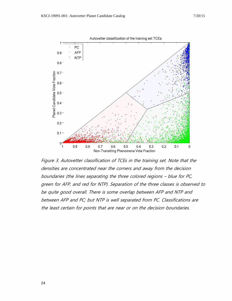
Figures 3 and 4 show ternary diagrams for the TCEs in the training set and TCEs of
previously unknown class. Since the PC, AFP and NTP vote fractions add to one, only
two are independent; we have chosen to display the NTP vote fraction along the abscissa
and the PC vote fraction along the ordinate axis. Perfect PC candidates would be at the
top right corner, perfect AFP candidates at the lower right corner, and perfect NTP
candidates at the lower left corner. The densities are generally concentrated toward the
corners of the triangle, and away from the decision boundaries (lines separating the
colored regions), which is the hallmark of a good classifier. Classifications are the least
certain for points that are near or on the decision boundaries.
KSCI-19091-001: Autovetter Planet Candidate Catalog 7/20/15
24
Figure 3. Autovetter classification of TCEs in the training set. Note that the
densities are concentrated near the corners and away from the decision
boundaries (the lines separating the three colored regions – blue for PC,
green for AFP, and red for NTP). Separation of the three classes is observed to
be quite good overall. There is some overlap between AFP and NTP and
between AFP and PC; but NTP is well separated from PC. Classifications are
the least certain for points that are near or on the decision boundaries.

KSCI-19091-001: Autovetter Planet Candidate Catalog 7/20/15
25
Figure 4. Autovetter classification of TCEs of UNKNOWN class. Again, the
densities are concentrated near the corners of the triangle and away from the
decision boundaries. Classifications are the least certain for points that are
near or on the decision boundaries.

KSCI-19091-001: Autovetter Planet Candidate Catalog 7/20/15
26
Histograms of posterior probability to be in the PC class are shown in Figures 5, 6, and 7
for TCEs that are classified as PC, AFP and NTP, respectively. Evidently, a TCE is
overwhelmingly likely to be a PC if classified as a PC, and overwhelmingly unlikely to
be a PC if not classified as a PC.
Figure 5. PC posterior probability for TCEs classified as PC. Most probabilities
are quite close to 1, though a narrow tail extends downward.

KSCI-19091-001: Autovetter Planet Candidate Catalog 7/20/15
27
Figure 6. PC posterior probability for TCEs classified as AFP. The probabilities
are concentrated near zero, though a narrow tail extends upward.

KSCI-19091-001: Autovetter Planet Candidate Catalog 7/20/15
28
8.3 Comparison of the Autovetter Catalog to the Robovetter Catalog
The robovetter is an expert system designed to automatically classify TCEs based on
heuristics developed by the TCERT team (see [Coughlin 2015]). The robovetter differs
from the autovetter in that its heuristics are (with the exception of the Locality Preserving
Projection) ‘hardwired’ by humans rather than ‘learned’ autonomously from the data. The
robovetter first decides if a TCE is Not Transit Like; these TCEs are excluded from
further consideration. The rest become KOIs, and are classified as either PC (planet
candidate), or FP (false positive). FPs are KOIs with transit-like signatures that analysis
has shown to be due to a star rather than a planet. Classifications by the robovetter have
been delivered to NExScI and can be found in the Q1-Q17 DR24 KOI table. In this
section we compare the autovetter catalog classifications against those of the robovetter
catalog.
8.3.1 Overall TCE Classifications
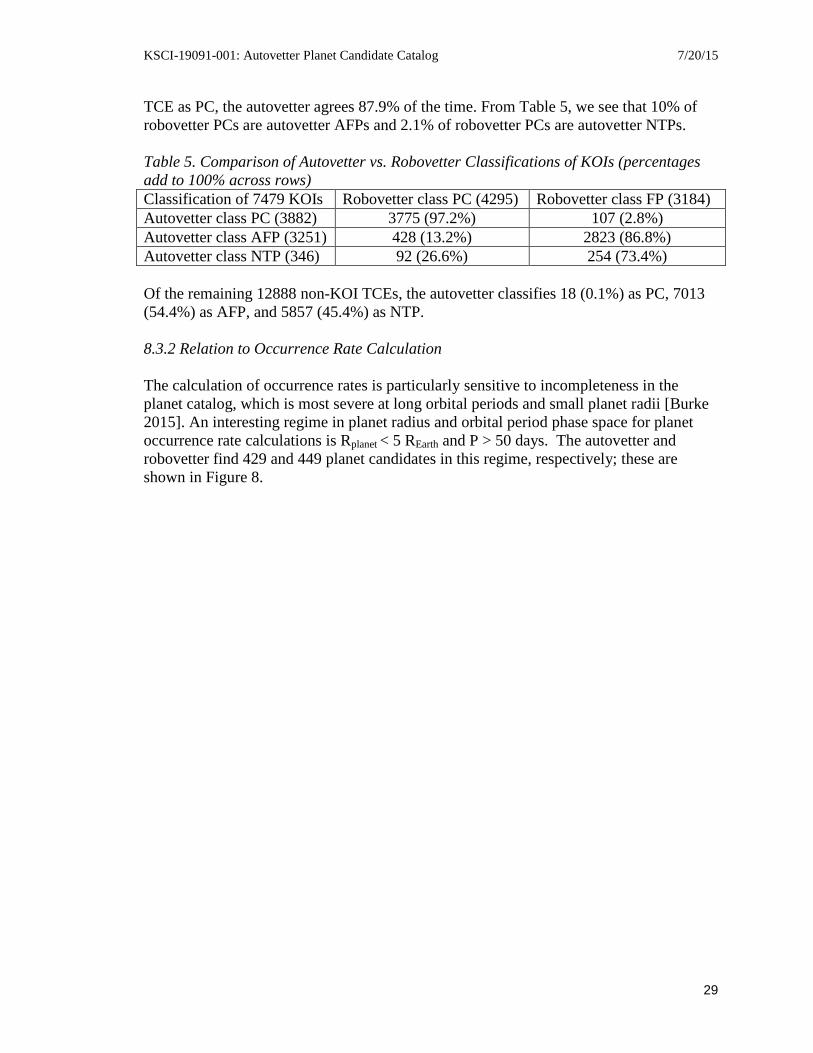
The full comparison for the 7479 KOIs is given in Table 5. When the autovetter classifies
a TCE as PC, the robovetter agrees 97.2% of the time. When the robovetter classifies a
Figure 7. PC posterior probability for TCEs classified as NTP. The probabilities
are concentrated near zero, though a narrow tail extends upward.
KSCI-19091-001: Autovetter Planet Candidate Catalog 7/20/15
29
TCE as PC, the autovetter agrees 87.9% of the time. From Table 5, we see that 10% of
robovetter PCs are autovetter AFPs and 2.1% of robovetter PCs are autovetter NTPs.
Table 5. Comparison of Autovetter vs. Robovetter Classifications of KOIs (percentages
add to 100% across rows)
Classification of 7479 KOIs Robovetter class PC (4295) Robovetter class FP (3184)
Autovetter class PC (3882) 3775 (97.2%) 107 (2.8%)
Autovetter class AFP (3251) 428 (13.2%) 2823 (86.8%)
Autovetter class NTP (346) 92 (26.6%) 254 (73.4%)
Of the remaining 12888 non-KOI TCEs, the autovetter classifies 18 (0.1%) as PC, 7013
(54.4%) as AFP, and 5857 (45.4%) as NTP.
8.3.2 Relation to Occurrence Rate Calculation
The calculation of occurrence rates is particularly sensitive to incompleteness in the
planet catalog, which is most severe at long orbital periods and small planet radii [Burke
2015]. An interesting regime in planet radius and orbital period phase space for planet
occurrence rate calculations is Rplanet < 5 REarth and P > 50 days. The autovetter and
robovetter find 429 and 449 planet candidates in this regime, respectively; these are
shown in Figure 8.

KSCI-19091-001: Autovetter Planet Candidate Catalog 7/20/15
30
Figure 8. Robovetter vs. autovetter planet candidates in a regime that affects
planetary occurrence rates. The robovetter has more candidates in the small
radius and long period region of phase space.
For each TCE, the autovetter provides a posterior probability that it is a member of the
class of PCs, which can be understood as a measure of the confidence, or reliability of the
classification. Figure 9 shows the PC posterior probabilities of the autovetter and
robovetter candidates from Figure 8. We expect that PCs in the low-SNR regime toward
long periods and smaller radii would tend to have smaller PC posterior probabilities than
other PCs; it is evident from Figure 9 that this is indeed the case.

KSCI-19091-001: Autovetter Planet Candidate Catalog 7/20/15
31
Figure 9. PC posterior probabilities for autovetter and robovetter planet
candidates smaller than 5 REarth and with orbit periods longer than 50 days.
Within this range there are 449 robovetter PCs and 429 autovetter PCs. In the
plot, the 416 PCs common to both robovetter and autovetter are represented
by filled squares, the 13 autovetter PCs that are not robovetter PCs are
represented by empty squares, and the 33 robovetter PCs that are not
autovetter PCs are represented by filled diamonds. Among autovetter PCs
(squares), the probabilities tend to be smaller for planets toward the long
period, small radius regime, indicating that these candidates are in general
less reliable than the others. The non-autovetter PCs have very small
autovetter PC posterior probabilities (filled diamonds).
8.3.3 Analysis of Robovetter Flags
The robovetter provides four flags that appear in the NExScI KOI activity tables:

KSCI-19091-001: Autovetter Planet Candidate Catalog 7/20/15
32
a) The Not Transit Like flag (NT) is set for TCEs whose light curves lack a transit
signature characteristic of a planet or detached eclipsing binary. This includes TCEs
with periodic light curve variations due to contact binaries, tidal binaries, starspots,
and pulsations, as well as noise artifacts.
b) The Significant Secondary flag (SS) indicates TCEs whose light curves have a
smaller ‘dip’ in the light curve that is characteristic of a secondary transit – a self-
luminous star (or planet) being occulted by the primary.
c) The Centroid Offset flag (CO) indicates TCEs whose in-transit centroid differs from
the out-of-transit centroid. This indicates that the transit signal originates from a star
other than the target star, such as a background eclipsing binary.
d) The Ephemeris Match flag (EM) is set if the TCE’s period and epoch were matched
to the ephemeris of another TCE, indicating that the putative transit signal is an
artifact induced by contamination.
TCEs whose light curves are periodic but not transit-like (such as sinusoidal variations)
tend to have the Not Transit Like flag (a) set, but the autovetter tends to classify them as
AFP. TCEs with flags (b) and (c) set will generally be classified as AFP by the
autovetter. For TCEs with flag (d) set, all but the ones contaminated with RR Lyrae or the
459-day systematic would tend to be classified as AFP by the autovetter (see discussion
in section 6).
Table 6 breaks out the autovetter classifications for TCEs with each of the robovetter
flags. The autovetter very rarely classifies TCEs with any of these flags as PCs. The
autovetter shows excellent agreement with the robovetter SS flag, classifying TCEs with
the SS flag as AFPs 96.8% of the time.
Table 6. Autovetter Classification of TCEs with Robovetter Flags
Autovetter PC Autovetter AFP Autovetter NTP
CO flag (2177) 42 (1.9%) 1866 (85.7%) 269 (12.4%)
SS flag (3131) 42 (1.3%) 3032 (96.8%) 57 (1.8%)
EM flag (1910) 10 (0.5%) 1336 (70.0%) 564 (29.5%)
NT flag (13258) 45 (0.3%) 7197 (54.3%) 6016 (45.4%)
8.4 Summary: Comparison of the Autovetter and Robovetter in Practice
The autovetter and robovetter have followed two distinct approaches to arrive at the same
goal – automation of the process of human classification of planet candidates to achieve
robust and consistent vetting of the entire population of TCEs. The robovetter is an
expert system that applies a set of explicit rules involving values of a focused set of
attributes to arrive at a classification decision. The rules are tuned and iterated by
knowledgeable experts to approximate a human decision, based on many individual
cases. The autovetter is a supervised machine learning classifier that derives an implicit
mapping between the values of a much broader set of attributes and a classification
decision. The learning is supervised because it relies on a training set of representative

KSCI-19091-001: Autovetter Planet Candidate Catalog 7/20/15
33
TCEs with labels (classifications) that are largely derived from humans and which we are
reasonably confident are true.
There are two chief differences between the resulting catalogs: the autovetter provides an
associated measure of confidence (posterior class probability) with each classification
(which the robovetter does not), and the robovetter provides a specific reason for each
classification (which the autovetter does not).
The posterior class probabilities ultimately derive from the relative votes of the random
forest for each class. Visualizing the votes on a ternary diagram can qualitatively indicate
the degree of confidence we should have in a classification by revealing whether a
particular TCE is well within a decision region or close to a corner (high confidence), or
is close to a decision boundary (lower confidence). The degree of confidence is
quantified in the form of a posterior probability that the TCE is a member of each of the
three classes. Posterior probabilities can be advantageously used in statistical studies such
as occurrence rate calculations to de-weight planet candidates that are at the noisy edges
of the planet catalog.
While the autovetter and robovetter agree on the classification of the vast majority of
PCs, they do not agree in every case. For example the autovetter tends to classify planets
that are large enough and bright enough to have secondary eclipses as AFPs, while the
robovetter is tuned to be able to identify them.
Another important difference is that while the autovetter has three classifications,
PC/AFP/NTP, the robovetter has four flags: Not Transit-Like, Significant Secondary,
Centroid Offset, and Ephemeris Match. These flags allow various sub-populations (e.g.,
on- and off-target EBs, off-target flux PCs, secondary eclipses) to be selected for further
study.

KSCI-19091-001: Autovetter Planet Candidate Catalog 7/20/15
34
9. References
[Batalha 2013] Batalha, N.M. et al. “Planetary Candidates Observed by Kepler III.
Analysis of the First 16 Months of Data”, 2013 ApJS, 204, 24
[Borucki 2011a] Borucki, W.J. et al. “Characteristics of Planetary Candidates Based on
the First Data Set”, 2011 ApJ, 728, 117
[Borucki 2011b] Borucki, W.J. et al. “Characteristics of Planetary Candidates Observed
by Kepler II. Analysis of the First Four Months of Data”, 2011 ApJ, 736, 19
[Breiman 2001] Breiman, L. “Random Forests”, 2001 Machine Learning, 45
[Burke 2014] Burke, C.J. et al. “Planetary Candidates Observed by Kepler IV. Planet
Sample from Q1-Q8 (22 months)”, 2014 ApJS, 210, 19
[Burke 2015] Burke, C.J. et al. “Terrestrial Planet Occurrence Rates for the Kepler GK
Dwarf Sample”, 2015 ApJ, accepted; arXiv:1506.04175
[Coughlin 2014] Coughlin, J. et al. “Contamination in the Kepler Field. Identification of
685 KOIs as false positives via ephemeris-matching based on Q1-Q12 data”, 2014 ApJ
147, 119
[Coughlin 2015] Coughlin, J. et al., “Planetary Candidates Observed by Kepler. VII. The
First Fully Automated Catalog Based on the Entire 48 Month Dataset (Q1-Q17 DR24)”,
2015 ApJ, in preparation.
[James 2013] James, G. et al. An Introduction to Statistical Learning, Springer 2013
[Jenkins 2010a] Jenkins, J. M., Caldwell, D. A., Chandrasekaran, H., et al. 2010,
ApJ, 713, L87
[Jenkins 2010b] Jenkins, J. M., Chandrasekaran, H., McCauliff, S. D., et al.
2010b, in Society of Photo-Optical Instrumentation Engineers (SPIE) Conference Series,
Vol. 7740
[Jenkins 2015a] Jenkins, J.M., Seader, S.E. and Burke, C.J., “Planet Detection Metrics:
Statistical Bootstrap Test”, 2015, KSCI-19086-001
[Jenkins 2015b] Jenkins, J.M. et al. “Discovery and validation of Kepler-7016b: A 1.6
REarth Super Earth Exoplanet in the Habitable Zone of a G2 Star”, 2015 ApJ, accepted.
[Jenkins 2015c] Jenkins, J.M. et al. “Automatic Classification of Kepler Threshold
Crossing Events: 363 New likely Kepler planetary candidates identified in the first 46
months”, 2015 ApJ, in preparation.

KSCI-19091-001: Autovetter Planet Candidate Catalog 7/20/15
35
[McCauliff 2015] McCauliff, S. D. et al. “Automatic Classification of Kepler Planetary
Transit Candidates”, 2015 ApJ 806, 6
[Mullally 2015] Mullally, F. et al. “Planetary Candidates Observed by Kepler VI. Planet
Sample from Q1-Q16 (47 Months)”, 2015 ApJS, 217, 31
[Rowe 2015] Rowe, J.F. et al. “Planetary Candidates Observed by Kepler V. Planet
Sample from Q1-Q12 (36 Months)”, 2015 ApJS, 217, 16
[Seader 2015] Seader, S.E. et al. “Detection of Potential Transit Signals in 17 Quarters of
Kepler Mission Data”, 2015 ApJS, 217, 18
[Thompson 2015] Thompson S. et al. “A Machine Learning Technique to Identify Transit
Shaped Signals”, 2015 ApJ, submitted.
[Wu 2010] Wu, H., Twicken, J. D., Tenenbaum, P., et al. 2010, in Society of Photo-
Optical Instrumentation Engineers (SPIE) Conference Series, Vol. 7740, Society of
Photo-Optical Instrumentation Engineers (SPIE) Conference Series, 19