Embed Size (px)
Citation preview

Autonomus Helicopter Landing on a Mobile Platform
Rasmus HansénNils LandinAxel Ringh
Victoria Svedberg
Supervisors:Xiaoming Hu Johan Markdahl
Degree Project in Engineering Physicsand Vehicle Engineering, SA104X and SA105X
Department of Mathematics, Optimization and Systems TheoryRoyal Institute of Technology
Stockholm, Sweden
Abstract
In this thesis we investigate the problem of landing a helicopter autonomously on a mobileplatform by designing controllers for the attitude- and translational dynamics in parallel. Amathematical model of the helicopter, in form of general 6-degrees-of-freedom rigid-body dy-namics with application-specific actuations, is developed. A linearized model is used in orderto make a landing problem more tractable, which is also rather reasonable under landing con-straints, where small angle- and velocity approximations are valid. The inputs used for theattitude controller are the tail rotor thrust and the tip-path-plane angles. Then, a form ofcascaded control is adopted for the translational dynamics, in which the inputs are the Eulerangles together with the main rotor thrust. The resulting control system is tested by MATLABsimulations against a smooth position reference path, with satisfying results. For the landingscenario, a trajectory planning strategy based on linear model predictive control (MPC) isadopted. The cascaded control system is then used to track the translational reference tra-jectory. The translational reference trajectory is chosen such that the attitude dynamics isadapted to the attitude of the platform at touch-down.
Sammanfattning
Den här uppsatsen undersöker problemet att autonomt landa en modellhelikopter på en mobilplattform genom att använda olika regulatorer för attityd- och translationsdynamiken. Denmatematiska beskrivningen av helikoptern utgår från dynamiken för en stel kropp med 6 fri-hetsgrader. Eftersom landning kan genomföras med låga hastigheter och små vinklar användsen linjär modell för att göra problemet mer lätthanterligt. Insignalerna till systemet är kraftenfrån stjärtrotorn och lutningsvinklarna av huvudrotorns Tip-Path-Plane. En kaskadregulatoranvänds för att styra translationssystemet med eulervinklarna och kraften från huvudrotorn,som insignaler. Regulatorn testas i en MATLAB-simulering mot en glatt referensbana medgodkända resultat. För landingsproceduren används en banplaneringsstrategi som bygger pålinjär prediktiv reglering (PR). Kaskadregulatorn används sedan för att följa translationsre-ferenserna, vilka blir valda så att även attitydsystemet anpassas efter plattformens attityd ilandningsögonblicket.
i
Nomenclature
0n×m The n×m matrix consisting of zeros
iB , jB , kB The body fixed unit vectors
iI , jI , kI The unit vectors in the inertial frame~fB The force affecting the helicopter expressed in the body frame~f I The force affecting the helicopter expressed in the inertial frame
a Angle of main rotor thrust vector, around jB
b Angle of main rotor thrust vector, around iB
g Gravitational acceleration
In×n The n-dimensional identity matrix
Ixx, Iyy, Izz Moments of inertia
Ixy, Ixz, Iyz Products of inertia
L, M , N External moment components in body fixed coordinates
m The mass of the helicopter
p, q, r Angular velocity components in body fixed coordinates
QM Reaction torque from the main rotor
R Rotation matrix from the body fixed frame to the inertial frame
sx, sy, sy The helicopters position
TM The thrust produced by the main rotor
TT The thrust produced by the tail rotor
u, v, w Velocity components in body fixed coordinates
X, Y , Z External force components in body fixed coordinates
xM , yM , zM The position of the main rotor in body fixed coordinates
xT , yT , zT The position of the tail rotor in body fixed coordinates
ii
φ Roll angle
Ψ Matrix relating the angular velocity and Euler angles to the time derivatives ofthe Euler angles
ψ Yaw angle
Θ A vector consisting of φ, θ and ψ
θ Pitch angle
~τB The torque affecting the helicopter expressed in the body frame
~τ I The torque affecting the helicopter expressed in the inertial frame
iii
Contents
1 Introduction 1
2 Mathematical Model of a Helicopter 32.1 Rigid body dynamics . . . . . . . . . . . . . . . . . . . . . . . . . . . . . . . . . . . . 3
2.1.1 Translational motion . . . . . . . . . . . . . . . . . . . . . . . . . . . . . . . . 42.1.2 Rotational motion . . . . . . . . . . . . . . . . . . . . . . . . . . . . . . . . . 42.1.3 Rotation matrix . . . . . . . . . . . . . . . . . . . . . . . . . . . . . . . . . . 52.1.4 Angular velocity . . . . . . . . . . . . . . . . . . . . . . . . . . . . . . . . . . 8
2.2 Forces and torques affecting the helicopter . . . . . . . . . . . . . . . . . . . . . . . . 92.2.1 The forces . . . . . . . . . . . . . . . . . . . . . . . . . . . . . . . . . . . . . . 102.2.2 The torques . . . . . . . . . . . . . . . . . . . . . . . . . . . . . . . . . . . . . 12
2.3 The dynamic equations of the helicopter . . . . . . . . . . . . . . . . . . . . . . . . . 132.3.1 Parameter values . . . . . . . . . . . . . . . . . . . . . . . . . . . . . . . . . . 13
3 Basic Control Theory 143.1 Basic concepts . . . . . . . . . . . . . . . . . . . . . . . . . . . . . . . . . . . . . . . 143.2 Stability . . . . . . . . . . . . . . . . . . . . . . . . . . . . . . . . . . . . . . . . . . . 163.3 State space description . . . . . . . . . . . . . . . . . . . . . . . . . . . . . . . . . . . 163.4 Controllability and observability . . . . . . . . . . . . . . . . . . . . . . . . . . . . . 183.5 State feedback . . . . . . . . . . . . . . . . . . . . . . . . . . . . . . . . . . . . . . . 193.6 MIMO-system . . . . . . . . . . . . . . . . . . . . . . . . . . . . . . . . . . . . . . . . 193.7 Linear quadratic control . . . . . . . . . . . . . . . . . . . . . . . . . . . . . . . . . . 20
4 Control Design 224.1 State space description . . . . . . . . . . . . . . . . . . . . . . . . . . . . . . . . . . . 234.2 Attitude controller . . . . . . . . . . . . . . . . . . . . . . . . . . . . . . . . . . . . . 23
4.2.1 Linearizing the system . . . . . . . . . . . . . . . . . . . . . . . . . . . . . . . 244.2.2 Set point control design . . . . . . . . . . . . . . . . . . . . . . . . . . . . . . 254.2.3 Tracking controller . . . . . . . . . . . . . . . . . . . . . . . . . . . . . . . . . 274.2.4 Simulations of the attitude controller . . . . . . . . . . . . . . . . . . . . . . . 284.2.5 Discussion . . . . . . . . . . . . . . . . . . . . . . . . . . . . . . . . . . . . . . 29
4.3 Translational controller . . . . . . . . . . . . . . . . . . . . . . . . . . . . . . . . . . 334.3.1 Controllability and choice of inputs . . . . . . . . . . . . . . . . . . . . . . . . 334.3.2 Tracking controller . . . . . . . . . . . . . . . . . . . . . . . . . . . . . . . . . 34
iv
CONTENTS
4.3.3 Feedforward control . . . . . . . . . . . . . . . . . . . . . . . . . . . . . . . . 344.3.4 Introducing integral action . . . . . . . . . . . . . . . . . . . . . . . . . . . . 354.3.5 Design of feedback gain . . . . . . . . . . . . . . . . . . . . . . . . . . . . . . 354.3.6 The complete attitude reference vector and differentiation . . . . . . . . . . . 36
4.4 Discussion . . . . . . . . . . . . . . . . . . . . . . . . . . . . . . . . . . . . . . . . . . 374.4.1 Review of model simplifications and exact trimming . . . . . . . . . . . . . . 37
5 Performance and Stability 415.1 Analytical path following . . . . . . . . . . . . . . . . . . . . . . . . . . . . . . . . . 415.2 Stability analysis . . . . . . . . . . . . . . . . . . . . . . . . . . . . . . . . . . . . . . 435.3 Disturbances . . . . . . . . . . . . . . . . . . . . . . . . . . . . . . . . . . . . . . . . 46
6 Landing Scenario 516.1 Landing premises . . . . . . . . . . . . . . . . . . . . . . . . . . . . . . . . . . . . . . 516.2 Trajectory generation . . . . . . . . . . . . . . . . . . . . . . . . . . . . . . . . . . . 52
6.2.1 Introduction to model predictive control (MPC) . . . . . . . . . . . . . . . . 526.2.2 Defining constraints and penalty matrices . . . . . . . . . . . . . . . . . . . . 556.2.3 Landing strategy . . . . . . . . . . . . . . . . . . . . . . . . . . . . . . . . . . 56
6.3 Discussion . . . . . . . . . . . . . . . . . . . . . . . . . . . . . . . . . . . . . . . . . . 576.3.1 Feasibility of the MPC . . . . . . . . . . . . . . . . . . . . . . . . . . . . . . . 576.3.2 Disturbances . . . . . . . . . . . . . . . . . . . . . . . . . . . . . . . . . . . . 586.3.3 Helicopter design and sensitivity to landing conditions . . . . . . . . . . . . . 58
7 Results and Conclusions 607.1 Simulation results . . . . . . . . . . . . . . . . . . . . . . . . . . . . . . . . . . . . . 607.2 Conclusions . . . . . . . . . . . . . . . . . . . . . . . . . . . . . . . . . . . . . . . . . 62
v
Chapter 1
Introduction
Unmanned Aerial Vehicles (UAVs) are flying objects that are being controlled without a pilot onboard. This definition emphasizes two important things about UAVs. First, they may take manydifferent shapes and are thus usable in many different settings. The earliest UAVs were developedfor intelligence gathering during the Gulf war since the traditional satellite spying methods werelimited by the satellite’s orbital period and manned flights were too risky [2]. Today, the militaryuse of UAVs extend to combat as well as intelligence. In a civilian setting UAVs may be usedfor rescue missions. Since UAVs do not need a pilot on board, they can be much smaller thanconventional aerial vehicles. Thus, UAVs may for example be used to stop leakages inside factoriesand small spaces. If the leakage is poisonous the UAV also has the advantage that no human needsto be exposed.
The second thing to observe is that the aerial vechicle is controlled without a pilot on board whichnot necessarily means that the flight is autonomous. Traditionally, radio control has been used tosteer UAVs, but in recent decades the control design of autonomous UAVs has been examined. Theadvantages of autonomous UAVs is that they can operate under conditions where the control signalis weak or at least stabilize themselves instead of crashing in the event of a signal failure. Fullautomation is also a first step to make the flying vehicles intelligent, which may reduce the costs ofpilot training in the future.
Today, the underlying mathematical model of small scale helicopters is well understood. In al-most all cases it is derived from the Newton-Euler equations for rigid body dynamics. A rigorousderivation is given by [13] and the resulting model is a multi-input multi-output (MIMO) non-linearsystem, i.e. a system with more than one input and output signals. Further the system’s parametersare highly coupled, thus making the control design more difficult.
As a concequence of the complexity in the system, linear control design is insufficient in providingstability for all flight envelopes. To solve this problem gain scheduling has been used, but at theexpense of higher computational loads [14]. For the purpose of making the helicopter hover a linearcontroller is sufficient since the helicopter is kept near one point in the state space [3].
Since landing is performed in conditions like those for hover flight, i.e. small velocities and angles,this thesis exploits the possibility to use linear control to land a helicopter. We constrain the
1
helicopter to small velocities and angles and assume that all state variables are measurable, whichresults in a faster and more reliable system. Further, the system’s inputs are the forces producedby the tail and main rotors as well as the tilt angle of the main rotor’s tip-path-plane. Thus, theaeorodynamics correlating the applied forces to the usual control inputs used to steer a helicopterare ignored. The result is again a faster and more reliable system. The platform is simulated tomove in a periodic motion like a ship at sea.
The rest of this report is organized as follows: In chapter 2 a mathematical model of the helicopteris derived from rigid body dynamics. Chapter 3 summarizes fundamental control theory which willbe used in the control design. In chapter 4 the design of the controller is presented. Chapter 5aims at testing the stability and performance properties of the derived controller by flying alonga smooth path as well as applying disturbances. Chapter 6 presents how the landing scenario arecarried out and a model predictive control is derived. The report ends with simulation results ofthe landing and conclusions in chapter 7.
2
Chapter 2
Mathematical Model of a Helicopter
The goal of this chapter is to develop a mathematical model of a small-scale helicopter. A helicopteris mathematically best modeled as a rigid body consisting of two power sources, the main- and tailrotors. This has been done in numerous articels in the field of Helicopter modelling, e.g in [13] and[12]. In the subsequent chapters the most important steps from these texts are reproduced to widenthe readers’ comprehension of the helicopter. First, general rigid body dynamics are presented andsecond these equations are adapted to the dynamics of the helicopter.
2.1 Rigid body dynamics
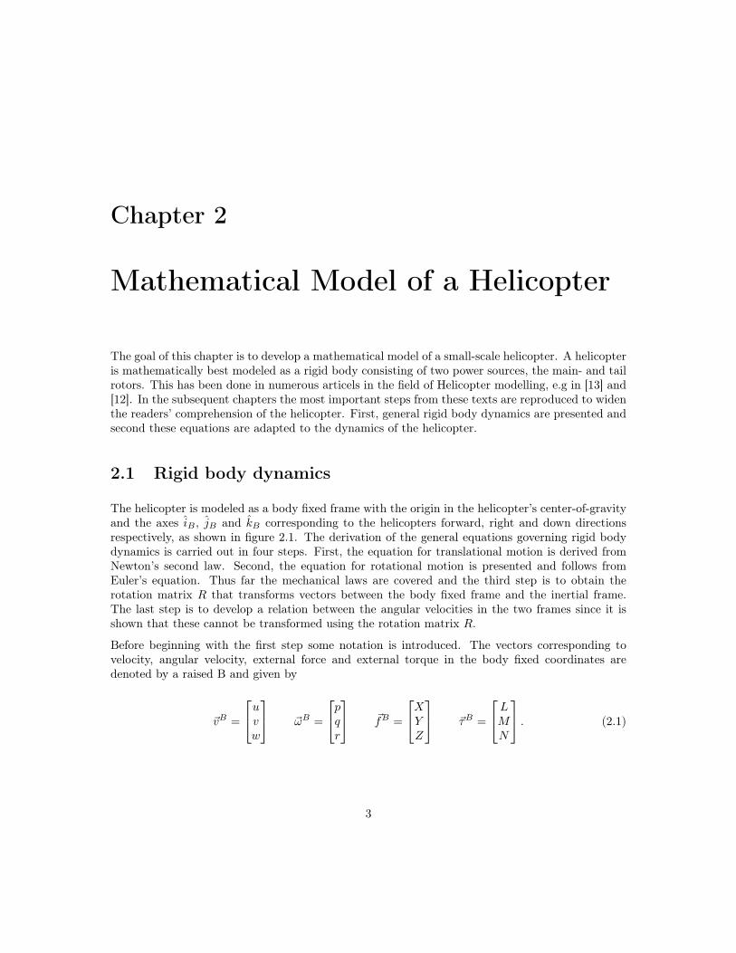
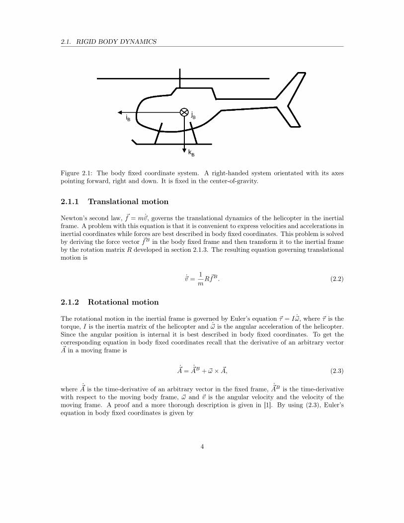
The helicopter is modeled as a body fixed frame with the origin in the helicopter’s center-of-gravityand the axes iB , jB and kB corresponding to the helicopters forward, right and down directionsrespectively, as shown in figure 2.1. The derivation of the general equations governing rigid bodydynamics is carried out in four steps. First, the equation for translational motion is derived fromNewton’s second law. Second, the equation for rotational motion is presented and follows fromEuler’s equation. Thus far the mechanical laws are covered and the third step is to obtain therotation matrix R that transforms vectors between the body fixed frame and the inertial frame.The last step is to develop a relation between the angular velocities in the two frames since it isshown that these cannot be transformed using the rotation matrix R.
Before beginning with the first step some notation is introduced. The vectors corresponding tovelocity, angular velocity, external force and external torque in the body fixed coordinates aredenoted by a raised B and given by
~vB =
uvw
~ωB =
pqr
~fB =
XYZ
~τB =
LMN
. (2.1)
3
2.1. RIGID BODY DYNAMICS
Figure 2.1: The body fixed coordinate system. A right-handed system orientated with its axespointing forward, right and down. It is fixed in the center-of-gravity.
2.1.1 Translational motion
Newton’s second law, ~f = m~v, governs the translational dynamics of the helicopter in the inertialframe. A problem with this equation is that it is convenient to express velocities and accelerations ininertial coordinates while forces are best described in body fixed coordinates. This problem is solvedby deriving the force vector ~fB in the body fixed frame and then transform it to the inertial frameby the rotation matrix R developed in section 2.1.3. The resulting equation governing translationalmotion is
~v =1
mR~fB . (2.2)
2.1.2 Rotational motion
The rotational motion in the inertial frame is governed by Euler’s equation ~τ = I~ω, where ~τ is thetorque, I is the inertia matrix of the helicopter and ~ω is the angular acceleration of the helicopter.Since the angular position is internal it is best described in body fixed coordinates. To get thecorresponding equation in body fixed coordinates recall that the derivative of an arbitrary vector~A in a moving frame is
~A = ~AB + ~ω × ~A, (2.3)
where ~A is the time-derivative of an arbitrary vector in the fixed frame, ~AB is the time-derivativewith respect to the moving body frame, ~ω and ~v is the angular velocity and the velocity of themoving frame. A proof and a more thorough description is given in [1]. By using (2.3), Euler’sequation in body fixed coordinates is given by
4
2.1. RIGID BODY DYNAMICS
~τB = I~ω = I~ωB + ~ωB × I~ωB ⇐⇒ I~ωB = ~τB − ~ωB × I~ωB . (2.4)
To finalize the description of the rotational motion it is assumed that the cross-terms Ixy, Ixz andIyz vanish, i.e. Ixy = Ixz = Iyz = 0. This is motivated by looking at the definitions of these terms:
Ixy =
∫body
xy dm, Iyz =
∫body
yz dm Ixz =
∫body
xz dm. (2.5)
Recall that the jB-direction (corresponding to the y-component in equations (2.5)) points to theright of the helicopter. If the helicopter is imagined as seen from its front, then it is easy to noticethat for each point (x, y, z) of the helicopter there is an identical point (x,−y, z). If the mass isevenly distributed across the helicopter, this motivates why Ixy = 0 and Iyz = 0. The equalityIxz = 0 is effected for simplistic reasons, but it poses no constraints to our model since it is possibleto adjust the weight distribution. This assumption is for example also done in [13], but not in [12].Under the assumption that the cross terms of the inertia matrix are zero, equation (2.4) can beextended to component form as
Ixxp = L− qr(Izz − Iyy),
Iyy q = M − pr(Ixx − Izz), (2.6)Izz r = N − pq(Iyy − Ixx).
2.1.3 Rotation matrix
To continue the development of the mechanical laws governing rigid body dynamics a method tocorrelate the body fixed system with the inertial system is derived. More precisely a tranformationbetween the two vector spaces spanned by {iB , jB , kB} and {iI , jI , kI} are obtained. The positionalrelation is simple since this is done by expressing the coordinates of the origin OB in inertial framecoordinates. The problem is how to relate the direction of vector properties in the two frames, e.g.forces and velocities. The solution is given by Euler’s rotation theorem [10].
Theorem 2.1.1. Any two independent orthonormal coordinate frames may be related by a minimumsequence of rotations (less than four) about coordinate axes, where no two successive rotations maybe about the same axis.
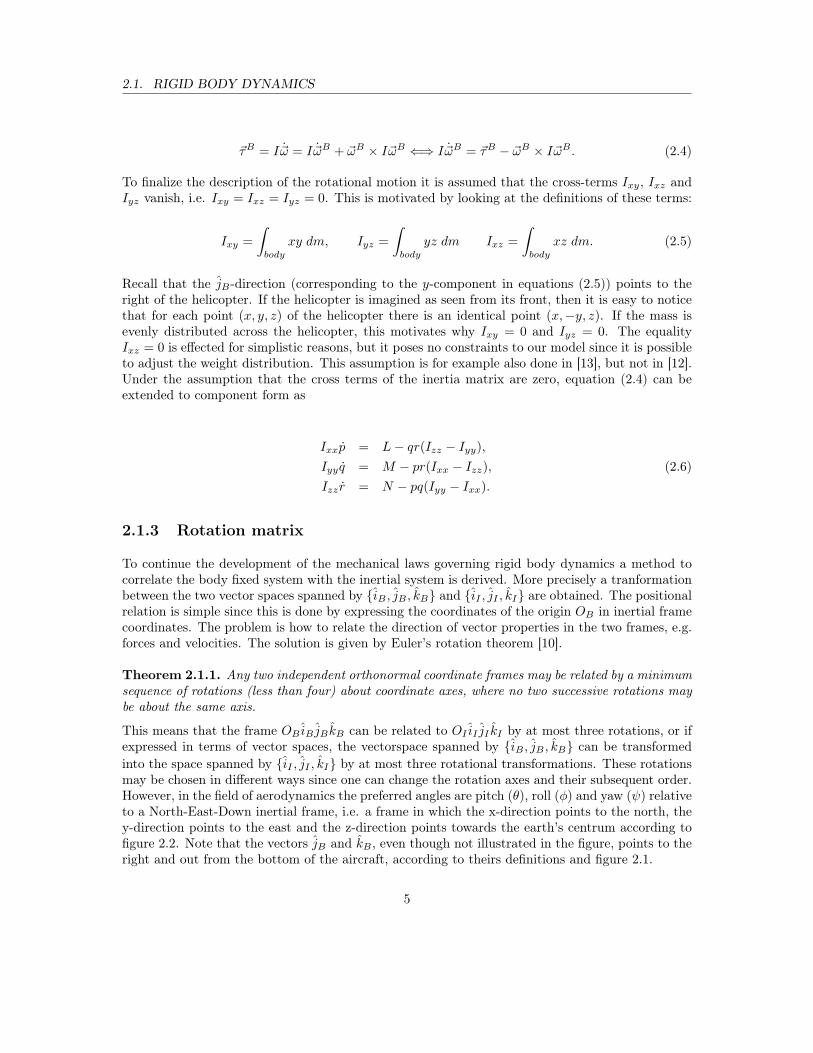
This means that the frame OB iB jB kB can be related to OI iI jI kI by at most three rotations, or ifexpressed in terms of vector spaces, the vectorspace spanned by {iB , jB , kB} can be transformedinto the space spanned by {iI , jI , kI} by at most three rotational transformations. These rotationsmay be chosen in different ways since one can change the rotation axes and their subsequent order.However, in the field of aerodynamics the preferred angles are pitch (θ), roll (φ) and yaw (ψ) relativeto a North-East-Down inertial frame, i.e. a frame in which the x-direction points to the north, they-direction points to the east and the z-direction points towards the earth’s centrum according tofigure 2.2. Note that the vectors jB and kB , even though not illustrated in the figure, points to theright and out from the bottom of the aircraft, according to theirs definitions and figure 2.1.
5
2.1. RIGID BODY DYNAMICS
The transformation between the spaces span{iI , jI , kI} and span{iB , jB , kB} is given by RT :
RT : {iI , jI , kI}Rψ(ψ)T−−−−−→ {a1, a2, a3}
Rθ(θ)T−−−−−→ {b1, b2, b3}Rφ(φ)T−−−−−→ {iB , jB , kB}
where the vector spaces span{a1, a2, a3} and span{b1, b2, b3} are some intermidate spaces andRψ(ψ)T , Rθ(θ)T and Rφ(φ)T correspond to the different rotational transformations as seen infigure 2.2. The transformations are transposed since it is more convenient to express the transfor-mation from the body fixed system to the inertial system by R. It can be proved, though it is notdone here, that RRT = I which implies that R is the desired transformation [13].
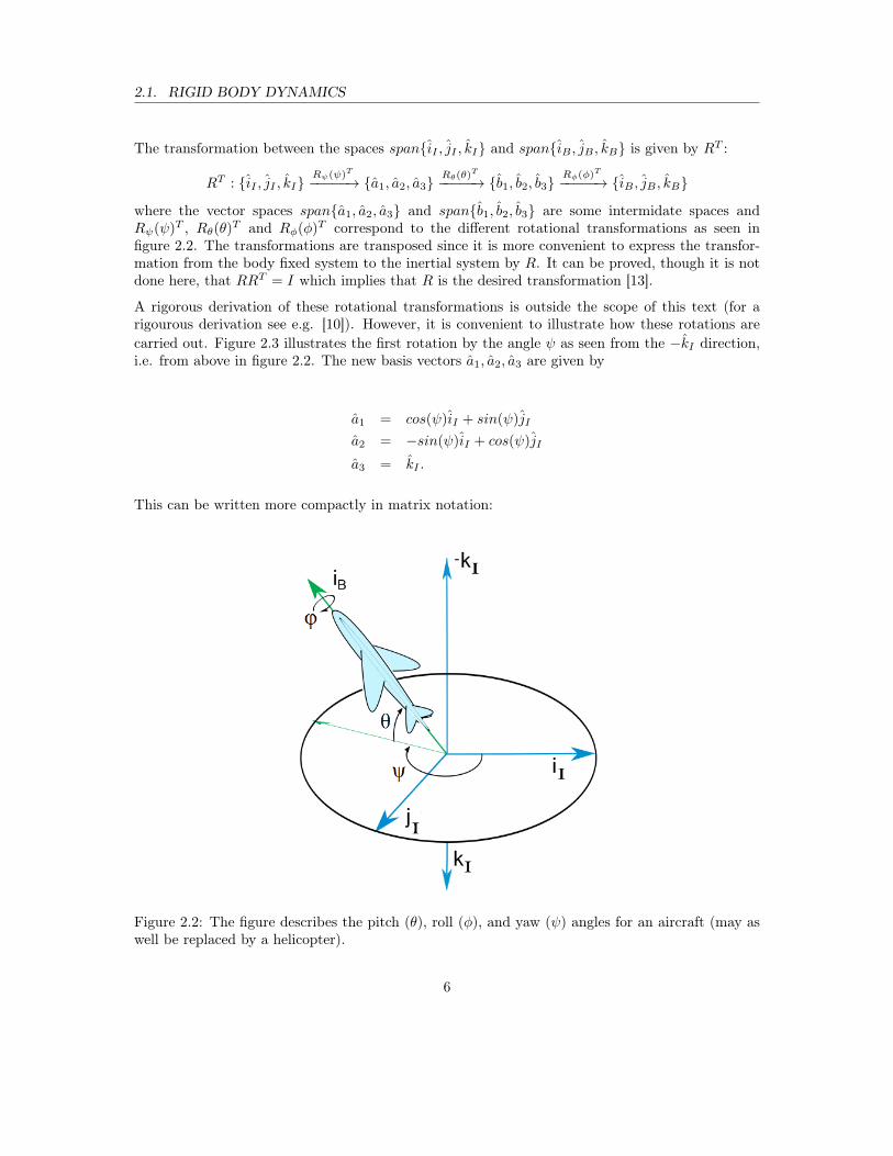
A rigorous derivation of these rotational transformations is outside the scope of this text (for arigourous derivation see e.g. [10]). However, it is convenient to illustrate how these rotations arecarried out. Figure 2.3 illustrates the first rotation by the angle ψ as seen from the −kI direction,i.e. from above in figure 2.2. The new basis vectors a1, a2, a3 are given by
a1 = cos(ψ)iI + sin(ψ)jI
a2 = −sin(ψ)iI + cos(ψ)jI
a3 = kI .
This can be written more compactly in matrix notation:
Figure 2.2: The figure describes the pitch (θ), roll (φ), and yaw (ψ) angles for an aircraft (may aswell be replaced by a helicopter).
6
2.1. RIGID BODY DYNAMICS
Figure 2.3: A rotation by ψ about the −kI axis pointing out of the paper.
a1
a2
a3
=
cos(ψ) sin(ψ) 0−sin(ψ) cos(ψ) 0
0 0 1
iIjIkI
= Rψ(ψ)T
iIjIkI
(2.7)
If the same geometric method are applied to the other two rotations, i.e. for Rθ(θ) and Rφ(φ), theresult is
b1b2b3
=
cos(θ) 0 −sin(θ)0 1 0
sin(θ) 0 cos(θ)
a1
a2
a3
= Rθ(θ)T
a1
a2
a3
(2.8)
and
iBjBkB
=
1 0 00 cos(φ) sin(φ)0 −sin(φ) cos(φ)
b1b2b3
= Rφ(φ)T
b1b2b3
. (2.9)
Finally, it follows that the rotation matrix from the inertial frame to the body fixed frame isRT = R(φ, θ, ψ)T = Rφ(φ)TRθ(θ)
TRψ(ψ)T and
7
2.1. RIGID BODY DYNAMICS
iBjBkB
= RT
iIjIkI
iIjIkI
= R
iBjBkB
(2.10)
2.1.4 Angular velocity
The last step in the derivation of the rigid body dynamics is the development of a relation betweenthe angular velocities in the two different frames. It is shown below that the angular velocity inthe inertial frame is given by ~ω = φiB + θa2 + ψkI . Since the Euler angles correspond to rotationsaround the axes kI , a2 and iB in three different frames, the rotation matrix in (2.10) cannot beused to transform this into the body fixed frame. Instead, the expressions for the angular velocityin the two frames are stated and then equated to get the desired relation. In body fixed coordinatesthe angular velocity is simply
~ω = piB + qjB + rkB =[iB jB kB
] pqr
. (2.11)
To obtain the angular velocity in the inertial frame, consider an infinitesimal change in the threeEuler angles dφ, dθ and dψ during the time dt. According to [13] this can be treated as a vector~h = dφiB+dθa2 +dψkI , where a2 is the basis vector explained in section 2.1.3. The angular velocityis then
~ω =d~h
dt= φiB + θa2 + ψkI =
[iB a2 kI
] φθψ
. (2.12)
By expressing[iB a2 kI
]=[iB jB kB
]Ψ−1 for some matrix Ψ−1, equation (2.12) can be written as
~ω =[iB jB kB
]Ψ−1
φθψ
(2.13)
and by equating the expressions (2.11) and (2.13), it follows that
pqr
= Ψ−1
φθψ
. (2.14)
The columns of the matrix Ψ−1 are the coordinates of iB , a2 and kI expressed in the body fixedframe. Thus, the first column is simply [1 0 0]
T . The second and third columns are derived by usingthe rotational transformations in the previous section. By equations (2.8) and (2.9) it follows that
8
2.2. FORCES AND TORQUES AFFECTING THE HELICOPTER
a1
a2
a3
= Rθ(θ)
b1b2b3
= Rθ(θ)Rφ(φ)
iBjBkB
. (2.15)
Since a2 is the second entry of the vector it can be expressed as the column vector
a2 =[iB jB kB
]Rφ(φ)TRθ(θ)
T
010
. (2.16)
Thus, the second column of Ψ−1 is Rφ(φ)TRθ(θ)T [0 1 0]
T . By the same steps and equation (2.10)it follows that kI can be written as
kI =[iB jB kB
]RT
001
. (2.17)
Thus, the third column of Ψ−1 is RT [0 0 1]T . Now, all the columns of Ψ−1 are derived and if the
multiplications are carried out the result is
Ψ−1 =
1 0 −sin(θ)0 cos(φ) sin(φ)cos(θ)0 −sin(φ) cos(φ)cos(θ)
. (2.18)
To get the derivatives of the Euler angles expressed in p, q and r the matrix Ψ−1 is inverted. Thisgives the relation ~Θ = Ψ~ωB , where ~Θ = [φ θ ψ]
T . Written out this becomes
φ
θ
ψ
=
p+ q sinφ tanθ + r cosφ tanθq cosφ− r sinφq sinφcosθ + r cosφcosθ
. (2.19)
2.2 Forces and torques affecting the helicopter
The equations (2.2) and (2.6), which were derived in the previous sections, constitute a generalmodel of a rigid body. The following section aims at specializing this model to helicopter dynamicsby developing a mathematical description of the force vector, ~fB , and torque vector, ~τB .
9
2.2. FORCES AND TORQUES AFFECTING THE HELICOPTER
2.2.1 The forces
The forces affecting the helicopter can be divided into three parts: thrust generated by the tail rotor,thrust generated by the main rotor and external forces. The thrust of the tail rotor is modeled asfollows. Let TT be the absolute value of the thrust and let ~TBT be the corresponding vector. Sincethe tail rotor is vertical it generates force in the jB-direction. Thus it follows that
~TBT =
0TT0
. (2.20)
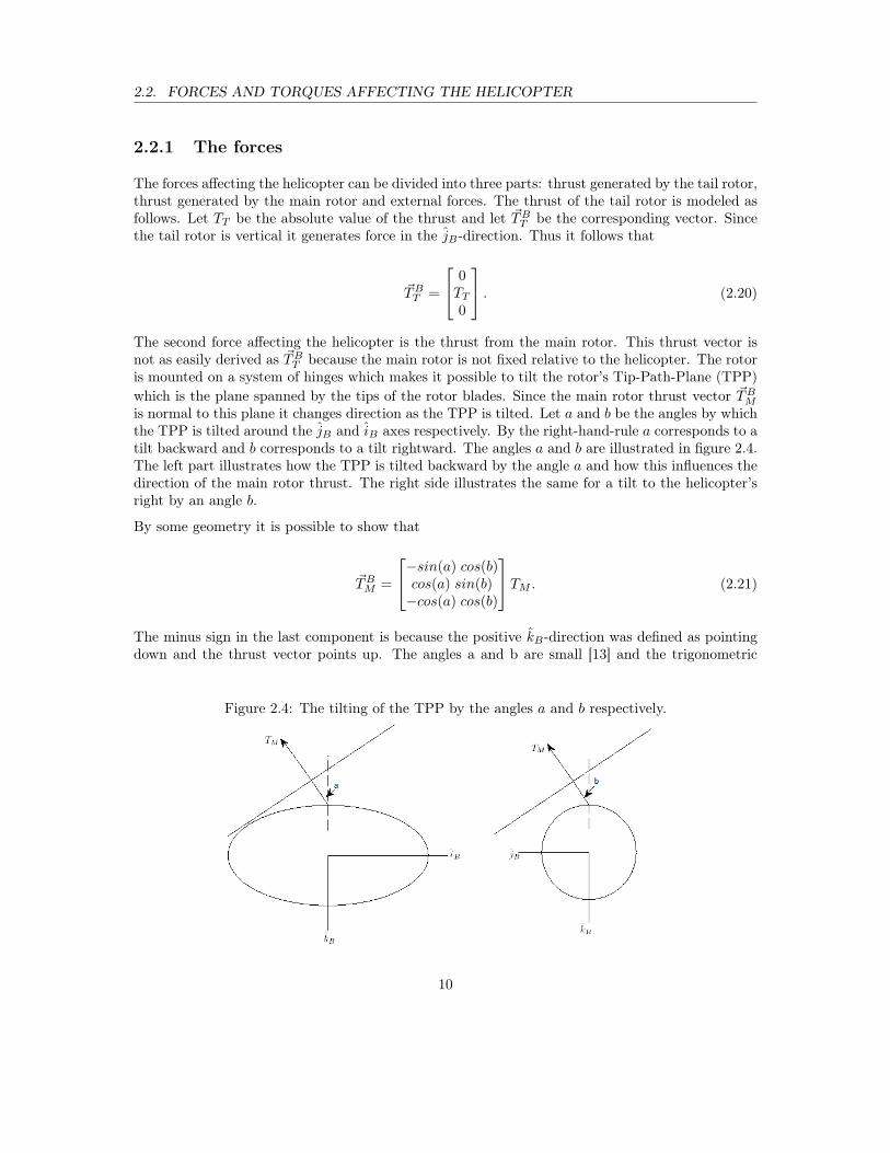
The second force affecting the helicopter is the thrust from the main rotor. This thrust vector isnot as easily derived as ~TBT because the main rotor is not fixed relative to the helicopter. The rotoris mounted on a system of hinges which makes it possible to tilt the rotor’s Tip-Path-Plane (TPP)which is the plane spanned by the tips of the rotor blades. Since the main rotor thrust vector ~TBMis normal to this plane it changes direction as the TPP is tilted. Let a and b be the angles by whichthe TPP is tilted around the jB and iB axes respectively. By the right-hand-rule a corresponds to atilt backward and b corresponds to a tilt rightward. The angles a and b are illustrated in figure 2.4.The left part illustrates how the TPP is tilted backward by the angle a and how this influences thedirection of the main rotor thrust. The right side illustrates the same for a tilt to the helicopter’sright by an angle b.
By some geometry it is possible to show that
~TBM =
−sin(a) cos(b)cos(a) sin(b)−cos(a) cos(b)
TM . (2.21)
The minus sign in the last component is because the positive kB-direction was defined as pointingdown and the thrust vector points up. The angles a and b are small [13] and the trigonometric
Figure 2.4: The tilting of the TPP by the angles a and b respectively.
10
2.2. FORCES AND TORQUES AFFECTING THE HELICOPTER
terms can therefore be approximated by sin(v) = v and cos(v) = 1 for v = a, b. The thrust vector(2.21) is therefore approximated by
~TBM =
−ab−1
TM . (2.22)
The third force affecting the helicopter is the external force which basically consists of three differentforces: gravitation, wind and drag. The gravitational force is always pointing down towards theearth’s centrum, i.e. in the kI -direction. Because the direction of the gravitation is given in inertialcoordinates, it must be transformed into the body fixed frame by using the rotation matrix RT in(2.10). This gives
~fBgrav = RT
00mg
. (2.23)
Wind and drag influence a rigid body in the same way since both are a consecuence of the helicoptersrelative motion to the air mass surrounding it. Of course the velocity of the wind is much morerandom and unforseen, but given a velocity it influences the body in the same way as drag. Ageneral model for the force produced on the body is [7]
D =1
2CDρAv
2 (2.24)
where D is the force on the object, ρ is the density of the air, v is the relative speed between thehelicopter and the air surrounding it, A is the effetctive area of the object facing the relative velocitygradient and CD is the drag coefficient, which depends on the geometric properies of the object.For a sphere CD = 0.47 [7]. For simplicity we will not consider drag in our model. Furthermore,winds will only be modeled as disturbances in the external forces. To be able to determine the sizeof the disturbances in the force, the helicopter will be modeled as a sphere with a radius zM , wherezM is the distance between the main rotor and the origin in the body fixed system (the helicopterscenter of gravity) in the kB-direction, which gives an effective area A = πz2
M . A normal value ofthe desity of air is ρ = 1.22kgm−3.
Now, all the forces (2.20), (2.22) and (2.23) can be put together to a force vector in body fixedcoordinates. It is given by
~fB =
−a TMb TM + TT−TM
+RT
00mg
.In [9] it is suggested that aTM , bTM and TT can be regarded as small compared to TM . With thisassumption it is possible to neglect these terms, which gives the following force vector:
11
2.2. FORCES AND TORQUES AFFECTING THE HELICOPTER
~fB =
00−TM
+RT
00mg
=
−mg sin(θ)mg cos(θ)sin(φ)
−TM +mg cos(θ)cos(φ)
. (2.25)
2.2.2 The torques
There are three sources which give rise to the torque on a helicopter which may be denoted by ~τBM ,~τBT and ~τBQ . The first two are due to the fact that the main and tail rotor thrusts not are alignedwith the center of gravity. The third is the reaction torque generated by the main rotor and atorque which results from the tilting of the TPP. These three sources are treated separatley below.
Let ~pM = [xM , yM , zM ] be the position of the main rotor in the body fixed frame. Then it followsfrom basic mechanics that
~τBM = ~pM × ~TBM =
yM ZM − zM YMzM XM − xM ZMxM YM − yM XM
(2.26)
where XM , YM and ZM are defined as the iB , jB and kB components of TBM respectively.
~τBT is derived in exactly the same way. Let ~pT = [xT , yT , zT ] be the position of the tail rotor inbody fixed coordinates. This gives that
~τBT = ~pM × ~TBT =
−zT TT0xT TT
. (2.27)
Both the reaction torque and the torque resulting from tilting the TPP follows from Newtons action-reaction law. The reaction torque is the reaction to the rotation of the main rotor. From empiricalresults [13] it follows that the value of the reaction torque tend to depend on |T 1.5
M | and is thusmodeled as QM = CM |T 1.5
M | + DM , where CM and DM are helicopter specific parameters whichmust be determined by empirical methods. It acts around the axis orthogonal to the TTP and thusit acts around the same axis as ~TBM , namely [−sin(a) cos(b), cos(a) sin(b),−cos(a) cos(b)]T . Sincethe angles a and b are assumed to be small, this can be approximated with [−a, b,−1]T .
The torque resulting from tilting the TPP is generated because the hinge around which the TPProtates has an internal stiffness. This stiffness tends to rotate the TPP back to its vertical position,thus generating a torque on the rotor. According to Newtons action-reaction law the same torquemust be generated on the helicopter. If the hinge is modeled as a spiral spring with stiffness Kβ ,the torque will be Kβa and Kβb around the axes jB and iB respectively. Combining equations theequations of this section results in the total moment
~τB =
−QMa− zmTMb+Kβb+ ztTT − ymTM−zmTMa+Kβa+QMb+ xmTMymTM a+ xmTMb+ xtTT −QM
. (2.28)
12
2.3. THE DYNAMIC EQUATIONS OF THE HELICOPTER
2.3 The dynamic equations of the helicopter
The expressions for the forces and moments acting on the helicopter that was derived in the previoussection, equations (2.25) and (2.28), can now be put into the general rigid body dynamic equationsfrom section 2.1, equations (2.2) and (2.6). This gives the dynamic equations
~vI =
sxsysz
=
−TMm (sin (φ) sin (ψ) + cos (φ) sin (θ) cos (ψ))TMm (sin (φ) cos (ψ)− cos (φ) sin (θ) sin (ψ))
1m (gm− cos (φ) cos (θ)TM )
(2.29)
and
I~ωB =
IxxpIyy qIzz r
=
−QMa+ (−zmTM +Kβ)b+ ztTT − ymTM − qr(Izz − Iyy)(−zmTM +Kβ)a+QMb+ xmTM − pr(Ixx − Izz)ymTMa+ xmTMb− xtTT −QM − pq(Iyy − Ixx)
. (2.30)
Together with equation (2.19), this constitutes a complete dynamic model of a small scale helicopter.From these equations it is observed that the complete system can be divided into translationaldynamics given by (2.29) and attitude dynamics given by (2.19) and (2.30).
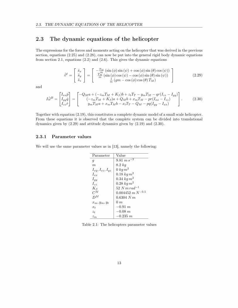
2.3.1 Parameter values
We will use the same parameter values as in [13], namely the following:
Parameter Valueg 9.81 ms−2
m 8.2 kgIxy, Ixz, Iyz 0 kgm2
Ixx 0.18 kgm2
Iyy 0.34 kgm2
Izz 0.28 kgm2
Kβ 52 N mrad−1
CM 0.004452 mN−0.5
DM 0.6304 N mxm, ym, yt 0 mxt −0.91 mzt −0.08 mzm −0.235 m
Table 2.1: The helicopters parameter values
13
Chapter 3
Basic Control Theory
Nowdays, dynamical systems are used to describe a variety of processes that are present in everydaylife. Using control theory we can influence the behavior of these system to act as preferred. Thiscould be the metabolism of a cell, the key rate proposed by a central bank or the software in anindustrial robot. In this chapter, a fundamental knowledge about control systems will be given inorder to fully understand the design of a regulator.
3.1 Basic concepts
Almost all dynamical system can be described, or at least approximated, by a set of differentialequations or difference equations which describes how a system behaves. Depending on how timeis described they are categorized into continuous and discrete systems. To solve these equationsone often applies the Z -transform on discrete systems and the Laplace-transform to a continuoussystems [6]. There are lots of similarities between the discrete and continuous case [5] so further ononly the later are treated.
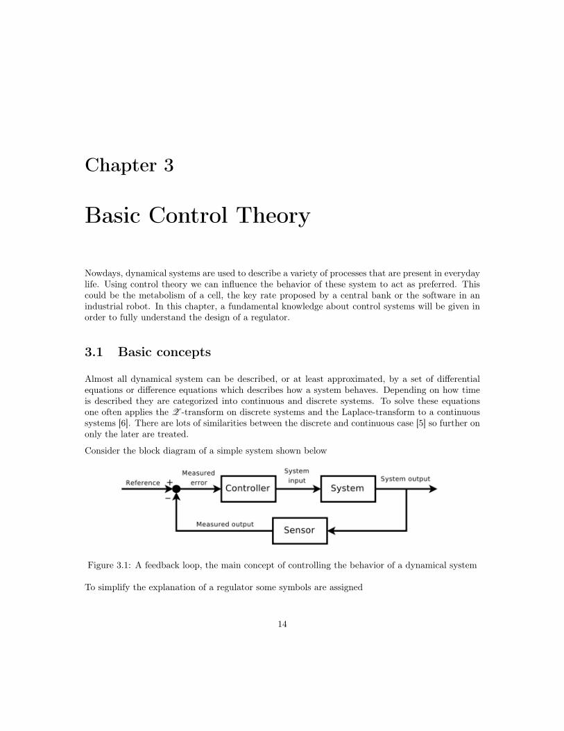
Consider the block diagram of a simple system shown below
Figure 3.1: A feedback loop, the main concept of controlling the behavior of a dynamical system
To simplify the explanation of a regulator some symbols are assigned
14
3.1. BASIC CONCEPTS
yref (t) = referencey(t) = system outpute(t) = yref − y = measured erroru(t) = system inputr(t) = controllerg(t) = weight functionf(t) = sensor
Depending on whether u and y are scalars or vectors, the system is a SISO-system (Single InputSingle Output) or a MIMO-system (Multiple Input Multiple Output). SISO- and MIMO-systemsshare many basic properties so for simplicity we choose to describe only SISO-systems here andlater translate it to a MIMO-system.
Most systems does not only depend on the input right now, but all the input signals the systemhas received since it was started. The system output y(t) is mathematically described as
y(t) =
∫ ∞−∞
g(τ)u(t− τ) dτ (3.1)
where g(t) is the systems weight function. It describes how differnet input signals in different timesare treated by the system.
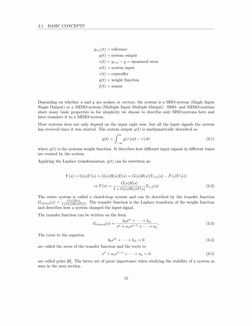
Applying the Laplace transformation, y(t) can be rewritten as:
Y (s) = G(s)U(s) = G(s)R(s)E(s) = G(s)R(s)(Yref (s)− F (s)Y (s))
⇒ Y (s) =G(s)R(s)
1 +G(s)R(s)F (s)Yref (s) (3.2)
The entire system is called a closed-loop system and can be described by the transfer functionGclosed(s) = G(s)R(s)
1+G(s)R(s)F (s) . The transfer function is the Laplace transform of the weight functionand describes how a system changed the input-signal.
The transfer function can be written on the form
Gclosed(s) =b0s
m + · · ·+ bmsn + a1sn−1 + · · ·+ an
, (3.3)
The roots to the equationb0s
m + · · ·+ bm = 0 (3.4)are called the zeros of the transfer function and the roots to
sn + a1sn−1 + · · ·+ an = 0 (3.5)
are called poles [6]. The latter are of great importance when studying the stability of a system asseen in the next section.
15
3.2. STABILITY
3.2 Stability
It is of vital importance to investigate whether the system is stable or not. In an unstable linearsystem, the output signal grows without bounds. This makes it impossible for the system to operateaccording to plan, why unstable linear system dynamics must be avoided. The following theorem arethe most fundamental to use in order to check the stability of a linear system and can be found in [6].
Theorem 3.2.1. A system is input-output stable if and only if the weight function g(t) satisfies∫ ∞0
|g(t)|dt <∞ .
Since the weight function is the inverse Laplace transform of the transfer function,
g(t) = L −1G(s), (3.6)
a criterion on the poles can be made instead [6].
Theorem 3.2.2. A system with the proper transfer function G(s) is input-output stable if andonly if all poles to G(s) have strict negative real parts.
Thus if one has a system where the poles all have negative real parts, the system is stable.
3.3 State space description
A general dynamical system does not only depend on the input at each time instance, but on allprevious input values. This can be seen from (3.1). Hence one can not tell how the system willreact by only looking at the current input signal. Therefore one introduces the term state. Aninformal definition of a systems state is: the information about the system needed to predict theeffect of an applied input signal [6].
A system is most often represented by a set of differential equations. The linear system y(n) +a1y
(n−1)(t) + · · ·+ an−2y(t) + an−1y(t) = bu(t) , where n is an arbitrary integer, can be rewrittenas:
y(n) = −a1y(n−1)(t)− · · · − an−2y(t)− an−1y(t) + bu(t) (3.7)
where y(n−1)(t0), . . . , y(t0), y(t0) and u(t0) are known. Thus we can calculate y(n)(t0) and alsoy(t0 + ∆), y(t0 + ∆), . . . , y(n−1)(t0 + ∆) for a infinitesimal ∆. It is of great convenience to rewritethe system on the form:
x1(t) = y(t)x2(t) = y(t) = x1
...xn(t) = y(n−1)(t)
(3.8)
16

3.3. STATE SPACE DESCRIPTION
xn(t) = y(n)(t) = −a1y(n−1)(t)− · · · − an−2y(t)− an−1y(t) + bu(t)
= −a1xn(t)− · · · − an−2x2(t)− an−1x1(t) + bu(t)
This can be written in matrix form as
x1(t)x2(t)...
xn−1(t)xn(t)
=
0 1 . . . 0 00 0 . . . 0 0...
.... . .
......
0 0 . . . 0 1−an−1 −an−2 . . . −a2 −a1
x1(t)x2(t)...
xn−1(t)xn(t)
+
00...0b
u(t) (3.9)
or short
~x(t) = A~x(t) +Bu(t)y(t) = C~x(t)
(3.10)
where
A =
0 1 . . . 0 00 0 . . . 0 0...
.... . .
......
0 0 . . . 0 1−an−1 −an−2 . . . −a2 −a1
, B =
00...0b
, C =
10...00
.This form is called a state space description of a linear dynamical system. Note that equation (3.10)is not a unique representation of equation (3.7). For any invertible matrix, T , the system inequation (3.11) is also a representation of equation (3.7).
~x = TAT−1~x+ TB~u
~y = CT−1~x+D~u.(3.11)
This non-uniqueness can be realized easiest by performing the following substitutions and compu-tations:
~x = T~x
⇒ ~x = T ~x
⇔ ~x = T (A~x+B~u)
⇔ ~x = T(AT−1~x+B~u
)= TAT−1~x+ TB~u
~y = C~x+D~u = CT−1~x+D~u.
This can be done for any invertible T and so there is an infinite number of representations with thesame input-output behaviour [6].
17
3.4. CONTROLLABILITY AND OBSERVABILITY
3.4 Controllability and observability
Controllability and observability are main issues when analyzing a system prior to deciding the bestcontrol strategy to be applied and it also decides whether it is possible to control or stabilize thesystem. Controllability is related to the possibility of forcing the system into a particular state byusing an appropriate control signal. If a state is not controllable, then no signal will ever be ableto control the state. The following formal definition can be found in [6].
Definition 3.4.1. A statevector ~x∗ is controllable if there exists an input, which takes the statefrom the origin to ~x∗ in a finite time interval. The system S is controllable if all the state vectorsare controllable.
Observability instead is related to the possibility of "observing", through output measurements,the state of a system. If not all states are directly measurable, but the system is observable, anobserver can be used to determine in which state the system is [6]. In our problem we assumethat all state variables are directly measurable and thus we do not need to use observers. Thediscussion of observability is therefore not relevant to the rest of this essay. It is included here forcompleteness.
The formal definition of observability can be found in [6]
Definition 3.4.2. A statevector ~x∗ 6= 0 is not observable if the output is identical zero when theinitial value is ~x∗ and the input identical zero. The system S is observable if all the state vectorsare observable.
If a system is given in state space description there are two nice theorems that determine if thesystem is controllable and observable. From [5] we have the theorem for controllability:
Theorem 3.4.1. The controllable states of a system in state space form, form a linear subspace,viz, the range of the matrix (the controllability matrix)
S (A,B) =[B AB . . . An−1B
]where n is the order of the system. The system is thus controllable if and only if S has full rank.
and the theorem for observability:
Theorem 3.4.2. The unobservable states of a system in state space form constitute a linear sub-space, viz, the null space of the matrix (the observability matrix)
O(A,C) =
CCA...
CAn−1
The system is thus observable if and only if O has full rank.
18
3.5. STATE FEEDBACK
3.5 State feedback
Sometimes it is convenient to let the input be decided by the state of the system, also called statefeedback. This section gives a short description of how this is done. Let the input signal be
u(t) = −L~x(t) + r (3.12)
where L = (l1, l2, ..., ln) and r(t) is a reference signal. If the system is written as
~x(t) = A~x(t) +Bu(t)y(t) = C~x(t)
(3.13)
then the feedback system is described by
~x(t) = (A−BL)~x(t) +Br(t)y(t) = C~x(t).
(3.14)
The poles to a system of the form (3.13) are given by the eigenvalues to the matrix A−BL. Sincethe poles determines if the system is input-output stable according to theorem 3.2.2 the followingtheorem is important [6].
Theorem 3.5.1. Given a closed system
~x(t) = (A−BL)~x(t) +Br(t)y(t) = C~x(t).
(3.15)
If and only if the system, (A,B), is controllable is it possible to choose L such that (A−BL) getsarbitrarily predefined eigenvalues.
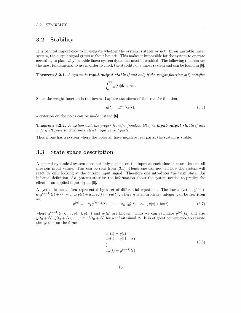
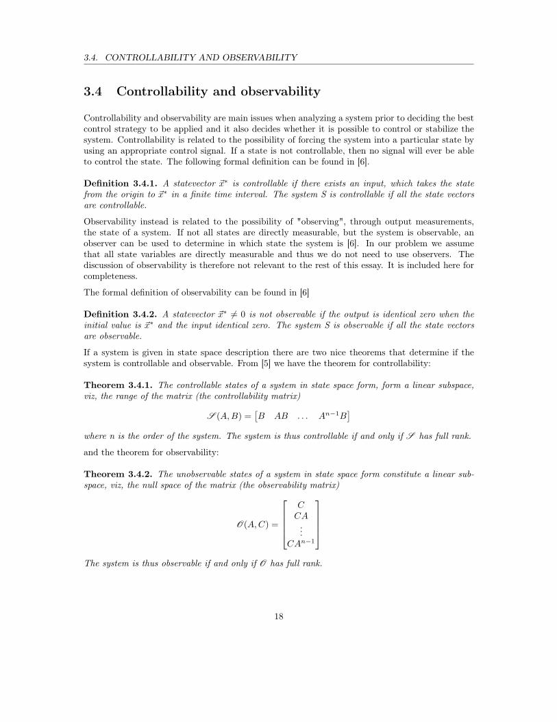
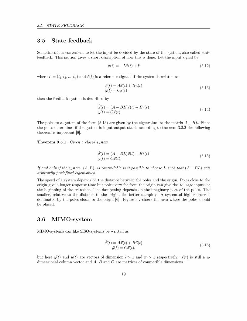
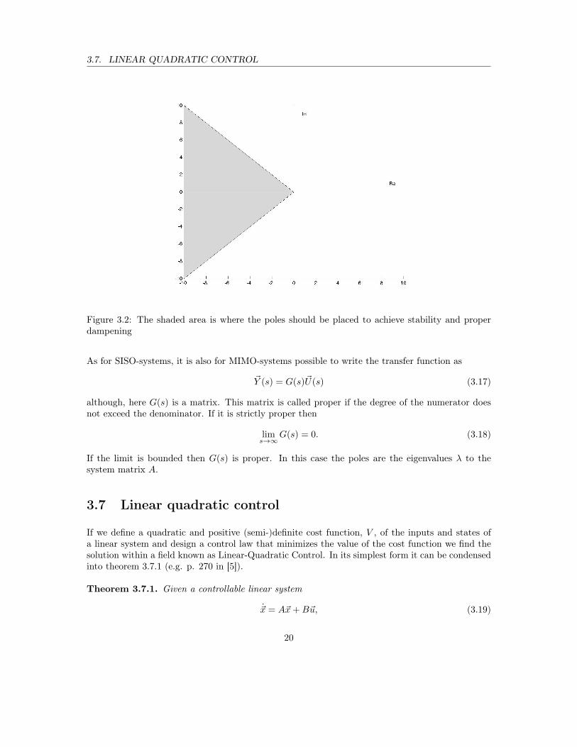
The speed of a system depends on the distance between the poles and the origin. Poles close to theorigin give a longer response time but poles very far from the origin can give rise to large inputs atthe beginning of the transient. The dampening depends on the imaginary part of the poles. Thesmaller, relative to the distance to the origin, the better damping. A system of higher order isdominated by the poles closer to the origin [6]. Figure 3.2 shows the area where the poles shouldbe placed.
3.6 MIMO-system
MIMO-systems can like SISO-systems be written as
~x(t) = A~x(t) +B~u(t)~y(t) = C~x(t),
(3.16)
but here ~y(t) and ~u(t) are vectors of dimension l × 1 and m × 1 respectively. ~x(t) is still a n-dimensional column vector and A, B and C are matrices of compatible dimensions.
19
3.7. LINEAR QUADRATIC CONTROL
Figure 3.2: The shaded area is where the poles should be placed to achieve stability and properdampening
As for SISO-systems, it is also for MIMO-systems possible to write the transfer function as
~Y (s) = G(s)~U(s) (3.17)
although, here G(s) is a matrix. This matrix is called proper if the degree of the numerator doesnot exceed the denominator. If it is strictly proper then
lims→∞
G(s) = 0. (3.18)
If the limit is bounded then G(s) is proper. In this case the poles are the eigenvalues λ to thesystem matrix A.
3.7 Linear quadratic control
If we define a quadratic and positive (semi-)definite cost function, V , of the inputs and states ofa linear system and design a control law that minimizes the value of the cost function we find thesolution within a field known as Linear-Quadratic Control. In its simplest form it can be condensedinto theorem 3.7.1 (e.g. p. 270 in [5]).
Theorem 3.7.1. Given a controllable linear system
~x = A~x+B~u, (3.19)
20
3.7. LINEAR QUADRATIC CONTROL
the feedback that minimizes
V =
∞∫0
(~xT ·Qx · ~x+ ~uT ·Qu · ~u)dt, (3.20)
where Qx � 0 and Qu � 0, is given by~u = −L~x, (3.21)
whereL = Q−1
u BTS (3.22)
and where S is the unique, positive semidefinite solution to
ATS + SA+Qx − SBQ−1u BTS = 0. (3.23)
Note that controllability is not a necessary property of a system for theorem 3.7.1 to apply but itis sufficient and is the system property that will be considered in this thesis. Note that Qu needsto be positive definite while Qx may be positive semi-definite.
21
Chapter 4
Control Design
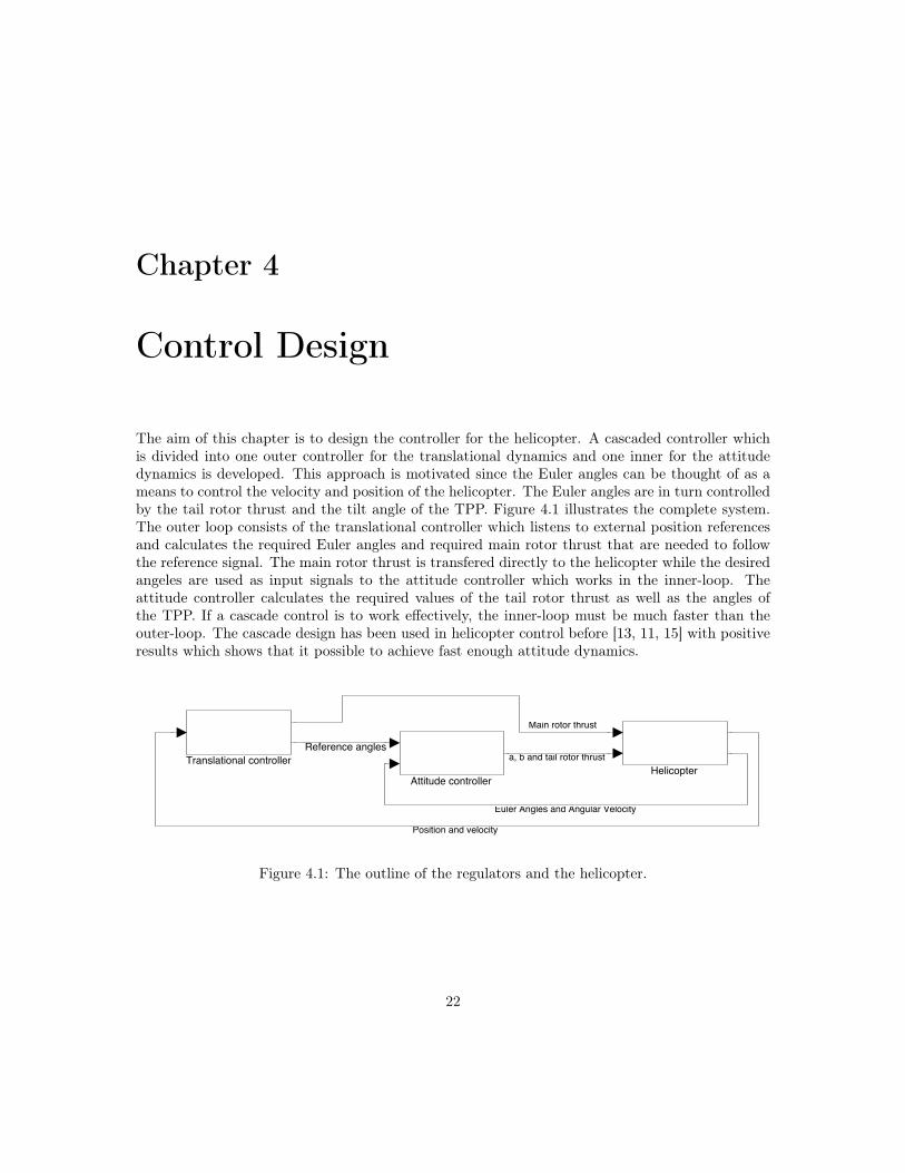
The aim of this chapter is to design the controller for the helicopter. A cascaded controller whichis divided into one outer controller for the translational dynamics and one inner for the attitudedynamics is developed. This approach is motivated since the Euler angles can be thought of as ameans to control the velocity and position of the helicopter. The Euler angles are in turn controlledby the tail rotor thrust and the tilt angle of the TPP. Figure 4.1 illustrates the complete system.The outer loop consists of the translational controller which listens to external position referencesand calculates the required Euler angles and required main rotor thrust that are needed to followthe reference signal. The main rotor thrust is transfered directly to the helicopter while the desiredangeles are used as input signals to the attitude controller which works in the inner-loop. Theattitude controller calculates the required values of the tail rotor thrust as well as the angles ofthe TPP. If a cascade control is to work effectively, the inner-loop must be much faster than theouter-loop. The cascade design has been used in helicopter control before [13, 11, 15] with positiveresults which shows that it possible to achieve fast enough attitude dynamics.
Reference anglesTranslational controller
HelicopterAttitude controller
a, b and tail rotor thrust
Main rotor thrust
Euler Angles and Angular Velocity
Position and velocity
Figure 4.1: The outline of the regulators and the helicopter.
22
4.1. STATE SPACE DESCRIPTION
4.1 State space description
Before the control design can be determined, the state space descriptions of the attitude andtranslational dynamics have to be obtained. The mathematical description of the helicopter wasdeveloped in chapter 2. As explained above, a cascade controller is going to be developed. Thus,separate state space descriptions are used for the translational and attitude dynamics. Accordingto the control design shown in figure 4.1 the following two systems are obtained:
{~xtr = ftr(~xtr, ~utr)~ytr = Ctr~xtr
(4.1){~xatt = fatt(~xatt, ~uatt)~yatt = Catt~xatt.
(4.2)
where the subscripts tr and att refers to translational and attitude respectively. From the divisionmotivated above it follows that the control vectors are given by ~uatt = [a, b, TT ]T and ~utr =[TM , φ, θ, ψ]T . The state space variables of the two different systems are ~xtr = [sx, sy, sz, sx, sy, sz]
T
and ~xatt = [φ, θ, ψ, p, q, r]T . The form of the functions ftr and fatt follows from the dynamicequations of the helicopter, equations (2.19), (2.29) and (2.30).
ftr(~xtr, ~utr) =
sxsysz
−TMm (sin (φ) sin (ψ) + cos (φ) sin (θ) cos (ψ))TMm (sin (φ) cos (ψ)− cos (φ) sin (θ) sin (ψ))
1m (gm− cos (φ) cos (θ)TM )
(4.3)
andfatt(~xatt, ~uatt) = fatt(~xatt) + gatt~uatt = (4.4)
p+ q · sinφ · tanθ + r · cosφ · tanθq · cosφ− r · sinφq ∗ sinφcosθ + r · cosφcosθ−ym·TM−q·r·(Izz−Iyy)
Ixxxm·TM−p·r·(Ixx−Izz)
Iyy−QM−p·q·(Iyy−Ixx)
Izz
+
0 0 00 0 00 0 0−QMIxx
−zm·TM+KβIxx
ztIxx
−zm·TM+KβIyy
QMIyy
0ym·TMIzz
xm·TMIzz
−xtIzz
~uatt.
Note that even though the main rotor thrust TM is part of (4.4), it is not treated as a state variableof the attitude system. Instead it is going to be treated as a scheduling variable.
4.2 Attitude controller
In this section two state feedback control laws for the attitude dynamics are designed. One law forset point control as well as one for tracking control. As shown above, the attitude system can bewritten as
23
4.2. ATTITUDE CONTROLLER
~xatt = fatt(~xatt) + gatt ~uatt. (4.5)
Inserting the parameter values, given in table 2.1, into the expressions gives
fatt(~xatt) =
p+ q sin (φ) tan (θ) + r cos (φ) tan (θ)
q cos (φ)− r sin (φ)
q sin(φ)cos(θ) + r cos(φ)
cos(θ)
13 qr
517 pr
− 257 QM − 4
7 pq
(4.6)
and
gatt =
0 0 0
0 0 0
0 0 0
− 509 QM
49 TM + 2600
9 − 49
4768 TM + 2600
175017 QM 0
0 0 134
. (4.7)
Since it is assumed that all state variables are measurable Catt = I6×6, and hence the output vectoris given by ~yatt = I6×6 ~xatt. The state space description is thus
{~xatt = fatt(~xatt) + gatt ~uatt~yatt = I6×6 ~xatt
(4.8)
4.2.1 Linearizing the system
In order to use linear control design the system (4.8) must be linearized. Since the vector fatt(~xatt)and matrix gatt depend on TM , both directly and indirectly through QM (QM = CM |TM |1.5 +DM ),gain scheduling must be used with TM as scheduling variable. However, as will be shown later, thesystem behaves well in the relevant operation range for TM with only one control law designed forthe case TM = mg.
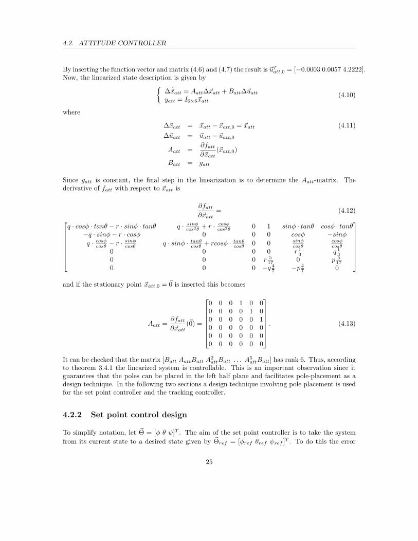
The linearization is done around a stationary point (~xatt,0, ~uatt,0) that is attained by solving theequation ~xatt = ~0. Since this thesis focus on the landing procedure during which the angles φ, θand ψ as well as the angular speeds p, q and r are assumed to be small, a linearization around thepoint ~xatt,0 = ~0 is preferable. With this choice of ~xatt,0 the equation ~xatt = ~0 is
~0 = fatt(~0) + g~uatt,0 ⇐⇒ ~uatt,0 = −g−1attfatt(~0) (4.9)
24
4.2. ATTITUDE CONTROLLER
By inserting the function vector and matrix (4.6) and (4.7) the result is ~uTatt,0 = [−0.0003 0.0057 4.2222].Now, the linearized state description is given by{
∆~xatt = Aatt∆~xatt +Batt∆~uattyatt = I6×6~xatt
(4.10)
where
∆~xatt = ~xatt − ~xatt,0 = ~xatt (4.11)∆~uatt = ~uatt − ~uatt,0
Aatt =∂fatt∂~xatt
(~xatt,0)
Batt = gatt
Since gatt is constant, the final step in the linearization is to determine the Aatt-matrix. Thederivative of fatt with respect to ~xatt is
∂fatt∂~xatt
= (4.12)q · cosφ · tanθ − r · sinφ · tanθ q · sinφcos2θ + r · cosφcos2θ 0 1 sinφ · tanθ cosφ · tanθ
−q · sinφ− r · cosφ 0 0 0 cosφ −sinφq · cosφcosθ − r ·
sinφcosθ q · sinφ · tanθcosθ + rcosφ · tanθcosθ 0 0 sinφ
cosθcosφcosθ
0 0 0 0 r 13 q 1
30 0 0 r 5
17 0 p 517
0 0 0 −q 47 −p 4
7 0
and if the stationary point ~xatt,0 = ~0 is inserted this becomes
Aatt =∂fatt∂~xatt
(~0) =
0 0 0 1 0 00 0 0 0 1 00 0 0 0 0 10 0 0 0 0 00 0 0 0 0 00 0 0 0 0 0
. (4.13)
It can be checked that the matrix [Batt AattBatt A2attBatt . . . A
5attBatt] has rank 6. Thus, according
to theorem 3.4.1 the linearized system is controllable. This is an important observation since itguarantees that the poles can be placed in the left half plane and facilitates pole-placement as adesign technique. In the following two sections a design technique involving pole placement is usedfor the set point controller and the tracking controller.
4.2.2 Set point control design
To simplify notation, let ~Θ = [φ θ ψ]T . The aim of the set point controller is to take the systemfrom its current state to a desired state given by ~Θref = [φref θref ψref ]T . To do this the error
25
4.2. ATTITUDE CONTROLLER
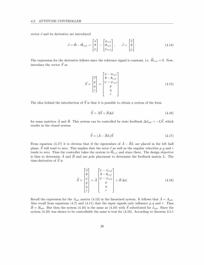
vector ~e and its derivative are introduced
~e = ~Θ− ~Θref =
φθψ
−φrefθrefψref
, ~e =
φθψ
. (4.14)
The expression for the derivative follows since the reference signal is constant, i.e. ~Θref = 0. Now,introduce the vector ~S as
~S =
~epqr
=
φ− φrefθ − θrefψ − ψref
pqr
(4.15)
The idea behind the introduction of ~S is that it is possible to obtain a system of the form
~S = A~S + B∆~u (4.16)
for some matrices A and B. This system can be controlled by state feedback ∆~uatt = −L~S, whichresults in the closed system
~S = (A− BL)~S. (4.17)
From equation (4.17) it is obvious that if the eigenvalues of A − BL are placed in the left halfplane, ~S will tend to zero. This implies that the error ~e as well as the angular velocities p, q and rtends to zero. Thus the controller takes the system to ~Θref and stays there. The design objectiveis thus to determine A and B and use pole placement to determine the feedback matrix L. Thetime-derivative of ~S is
~S =
φ
θ
ψpqr
= A
ψ − ψrefθ − θrefψ − ψref
pqr
+ B∆~u. (4.18)
Recall the expression for the Aatt matrix (4.13) in the linearized system. It follows that A = Aatt.Also recall from equations (4.7) and (4.11) that the input signals only influence p, q and r. ThusB = Batt. But then the system (4.16) is the same as (4.10) with ~S substituted for ~xatt. Since thesystem (4.10) was shown to be controllable the same is true for (4.16). According to theorem 3.5.1
26
4.2. ATTITUDE CONTROLLER
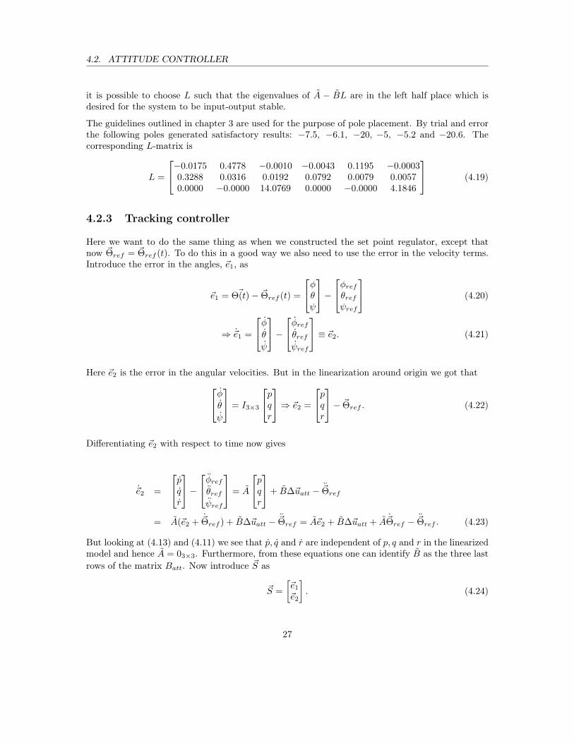
it is possible to choose L such that the eigenvalues of A − BL are in the left half place which isdesired for the system to be input-output stable.
The guidelines outlined in chapter 3 are used for the purpose of pole placement. By trial and errorthe following poles generated satisfactory results: −7.5, −6.1, −20, −5, −5.2 and −20.6. Thecorresponding L-matrix is
L =
−0.0175 0.4778 −0.0010 −0.0043 0.1195 −0.00030.3288 0.0316 0.0192 0.0792 0.0079 0.00570.0000 −0.0000 14.0769 0.0000 −0.0000 4.1846
(4.19)
4.2.3 Tracking controller
Here we want to do the same thing as when we constructed the set point regulator, except thatnow ~Θref = ~Θref (t). To do this in a good way we also need to use the error in the velocity terms.Introduce the error in the angles, ~e1, as
~e1 = ~Θ(t)− ~Θref (t) =
φθψ
−φrefθrefψref
(4.20)
⇒ ~e1 =
φθψ
−φrefθrefψref
≡ ~e2. (4.21)
Here ~e2 is the error in the angular velocities. But in the linearization around origin we got thatφθψ
= I3×3
pqr
⇒ ~e2 =
pqr
− ~Θref . (4.22)
Differentiating ~e2 with respect to time now gives
~e2 =
pqr
−φrefθrefψref
= A
pqr
+ B∆~uatt − ~Θref
= A(~e2 + ~Θref ) + B∆~uatt − ~Θref = A~e2 + B∆~uatt + A~Θref − ~Θref . (4.23)
But looking at (4.13) and (4.11) we see that p, q and r are independent of p, q and r in the linearizedmodel and hence A = 03×3. Furthermore, from these equations one can identify B as the three lastrows of the matrix Batt. Now introduce ~S as
~S =
[~e1
~e2
]. (4.24)
27
4.2. ATTITUDE CONTROLLER
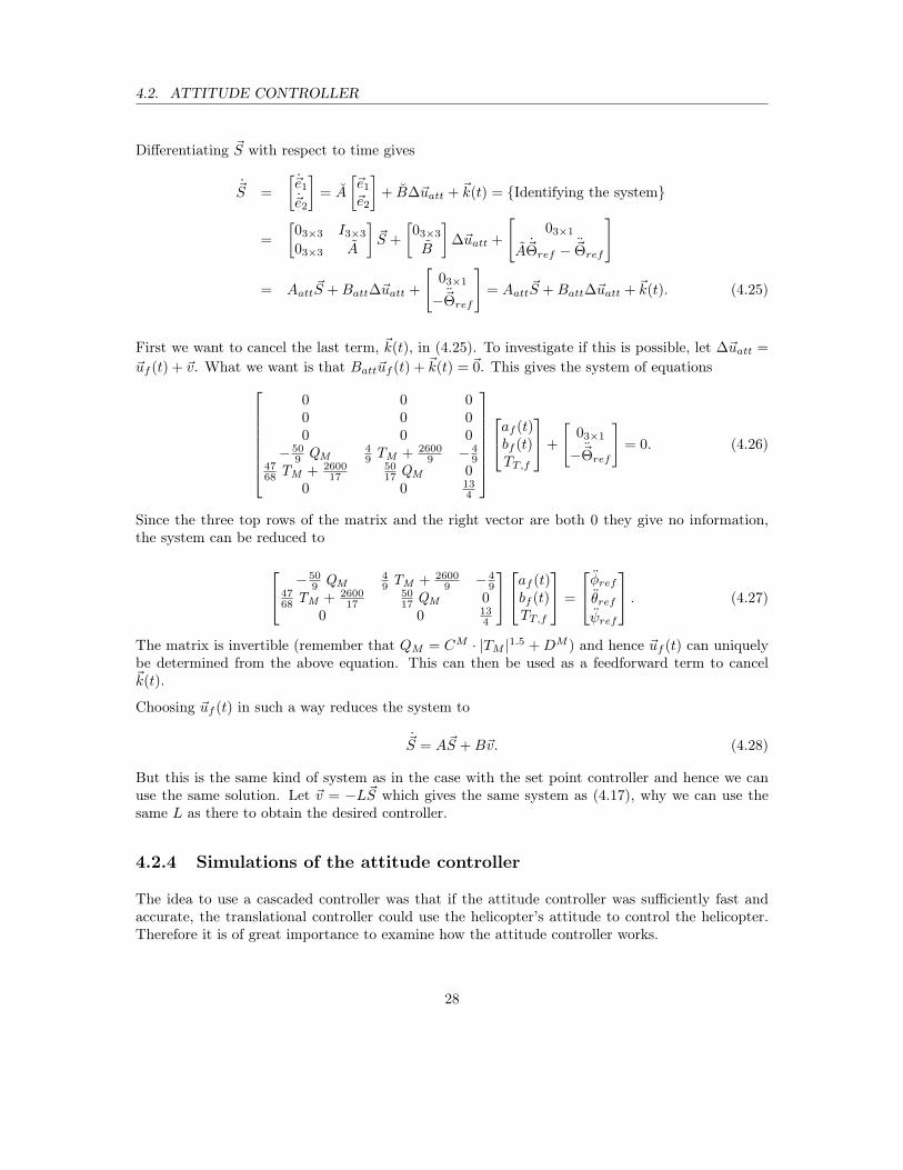
Differentiating ~S with respect to time gives
~S =
[~e1
~e2
]= A
[~e1
~e2
]+ B∆~uatt + ~k(t) = {Identifying the system}
=
[03×3 I3×3
03×3 A
]~S +
[03×3
B
]∆~uatt +
[03×1
A~Θref − ~Θref
]
= Aatt~S +Batt∆~uatt +
[03×1
−~Θref
]= Aatt~S +Batt∆~uatt + ~k(t). (4.25)
First we want to cancel the last term, ~k(t), in (4.25). To investigate if this is possible, let ∆~uatt =
~uf (t) + ~v. What we want is that Batt~uf (t) + ~k(t) = ~0. This gives the system of equations0 0 00 0 00 0 0
− 509 QM
49 TM + 2600
9 − 49
4768 TM + 2600
175017 QM 0
0 0 134
af (t)bf (t)TT,f
+
[03×1
−~Θref
]= 0. (4.26)
Since the three top rows of the matrix and the right vector are both 0 they give no information,the system can be reduced to
− 509 QM
49 TM + 2600
9 − 49
4768 TM + 2600
175017 QM 0
0 0 134
af (t)bf (t)TT,f
=
φrefθrefψref
. (4.27)
The matrix is invertible (remember that QM = CM · |TM |1.5 +DM ) and hence ~uf (t) can uniquelybe determined from the above equation. This can then be used as a feedforward term to cancel~k(t).
Choosing ~uf (t) in such a way reduces the system to
~S = A~S +B~v. (4.28)
But this is the same kind of system as in the case with the set point controller and hence we canuse the same solution. Let ~v = −L~S which gives the same system as (4.17), why we can use thesame L as there to obtain the desired controller.
4.2.4 Simulations of the attitude controller
The idea to use a cascaded controller was that if the attitude controller was sufficiently fast andaccurate, the translational controller could use the helicopter’s attitude to control the helicopter.Therefore it is of great importance to examine how the attitude controller works.
28
4.2. ATTITUDE CONTROLLER
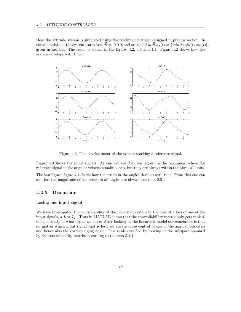
Here the attitude system is simulated using the tracking controller designed in previus section. Inthese simulations the system starts from ~Θ = [0 0 0] and are to follow ~Θref (t) = 1
2 [sin(t) sin(t) sin(t)] ,given in radians. The result is shown in the figures 4.2, 4.3 and 4.4. Figure 4.2 shows how thesystem develops with time.
Figure 4.2: The developtment of the system tracking a reference signal.
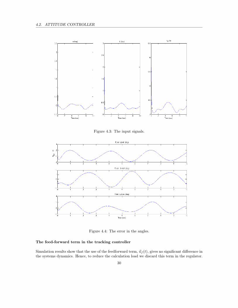
Figure 4.3 shows the input signals. As one can see they are lagrest in the beginning, where thereference signal in the angular velocities make a step, but they are always within the physical limits.
The last figure, figure 4.4 shows how the errors in the angles develop with time. From this one cansee that the magnitude of the errors in all angles are always less than 2.5◦.
4.2.5 Discussion
Losing one input signal
We have investigated the controllability of the linearized system in the case of a loss of one of theinput signals, a, b or TT . Tests in MATLAB shows that the controllabillity matrix only gets rank 4,independently of what signal we loose. After looking at the linearized model our conclusion is thatno matter which input signal that is lost, we always loose control of one of the angular velocitiesand hence also the corresponging angle. This is also verified by looking at the subspace spannedby the controllability matrix, according to theorem 3.4.1.
29
4.2. ATTITUDE CONTROLLER
Figure 4.3: The input signals.
Figure 4.4: The error in the angles.
The feed-forward term in the tracking controller
Simulation results show that the use of the feedforward term, ~uf (t), gives no significant difference inthe systems dynamics. Hence, to reduce the calculation load we discard this term in the regulator.
30
4.2. ATTITUDE CONTROLLER
This almost turns the trackning controller into the set point controller. The only difference is thatthe reference angular velocities are not set to zero.
Gain scheduling
As was noted earlier, the attitude system is depended of TM which is not a state space variable.Gain scheduling is one way of handling this. Expressed in an easy way, in this method you designdifferent regulators for a number of different operating points. Then you use a so called schedulingvarible to determine which controller is to be used [8]. In our case this would mean that we design anumber of regulators for different values of TM and then use TM as scheduling variable to determinewhich one to use.
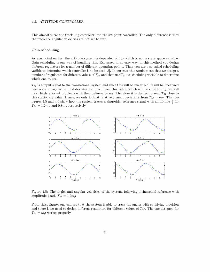
TM is a input signal to the translational system and since this will be linearized, it will be linearizednear a stationary value. If it deviates too much from this value, which will be close to mg, we willmost likely also get problems with the nonlinear terms. Therefore it is desired to keep TM close tothis stationary value. Hence, we only look at relatively small deviations from TM = mg. The twofigures 4.5 and 4.6 show how the system tracks a sinusoidal reference signal with amplitude 1
2 forTM = 1.2mg and 0.8mg respectively.
Figure 4.5: The angles and angular velocities of the system, following a sinusoidal reference withamplitude 1
2 rad. TM = 1.2mg
From these figures one can see that the system is able to track the angles with satisfying precisionand there is no need to design different regulators for different values of TM . The one designed forTM = mg workes properly.
31
4.2. ATTITUDE CONTROLLER
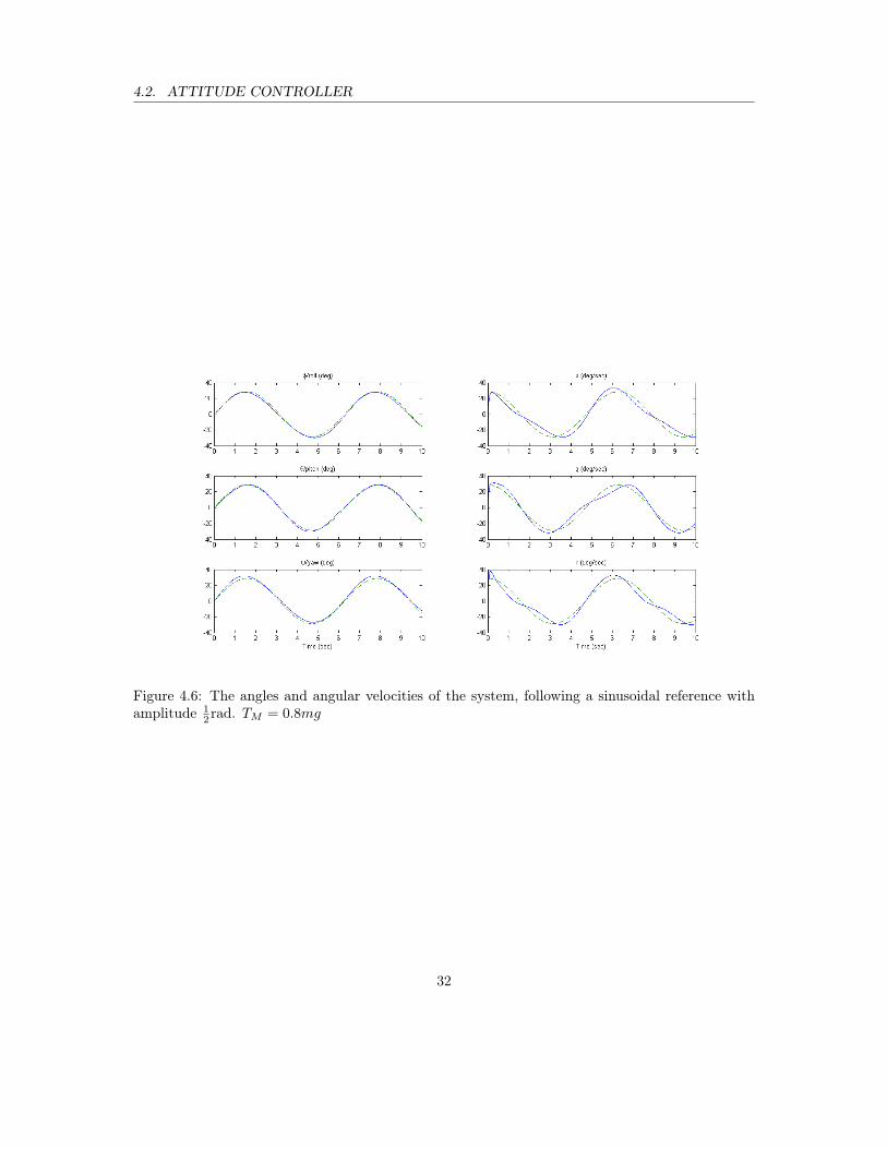
Figure 4.6: The angles and angular velocities of the system, following a sinusoidal reference withamplitude 1
2 rad. TM = 0.8mg
32
4.3. TRANSLATIONAL CONTROLLER
4.3 Translational controller
4.3.1 Controllability and choice of inputs
Ideally the choice to partition the state space in two regions, each to be controlled by a separate con-troller, would yield two controllable subsystems. However, with ~utr = Tm and ~uatt =
[a b Tt
]Twe get the controllability matrix for the translational subsystem to be
Str =
000
2.59 · 10−6
−6.39 · 10−3
−1.22 · 10−1
2.59 · 10−6
−6.39 · 10−3
−1.22 · 10−1
000
06×4
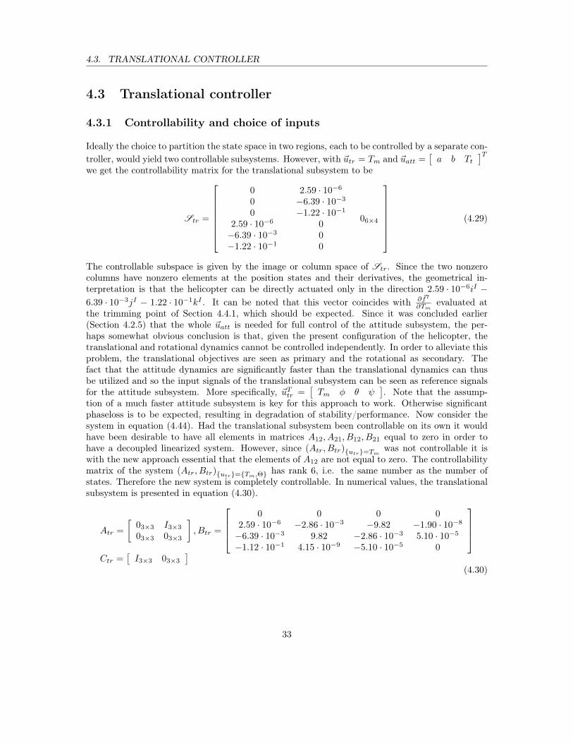
(4.29)
The controllable subspace is given by the image or column space of Str. Since the two nonzerocolumns have nonzero elements at the position states and their derivatives, the geometrical in-terpretation is that the helicopter can be directly actuated only in the direction 2.59 · 10−6iI −6.39 · 10−3jI − 1.22 · 10−1kI . It can be noted that this vector coincides with ∂ ~fI
∂Tmevaluated at
the trimming point of Section 4.4.1, which should be expected. Since it was concluded earlier(Section 4.2.5) that the whole ~uatt is needed for full control of the attitude subsystem, the per-haps somewhat obvious conclusion is that, given the present configuration of the helicopter, thetranslational and rotational dynamics cannot be controlled independently. In order to alleviate thisproblem, the translational objectives are seen as primary and the rotational as secondary. Thefact that the attitude dynamics are significantly faster than the translational dynamics can thusbe utilized and so the input signals of the translational subsystem can be seen as reference signalsfor the attitude subsystem. More specifically, ~uTtr =
[Tm φ θ ψ
]. Note that the assump-
tion of a much faster attitude subsystem is key for this approach to work. Otherwise significantphaseloss is to be expected, resulting in degradation of stability/performance. Now consider thesystem in equation (4.44). Had the translational subsystem been controllable on its own it wouldhave been desirable to have all elements in matrices A12, A21, B12, B21 equal to zero in order tohave a decoupled linearized system. However, since (Atr, Btr){utr}=Tm was not controllable it iswith the new approach essential that the elements of A12 are not equal to zero. The controllabilitymatrix of the system (Atr, Btr){utr}={Tm,Θ} has rank 6, i.e. the same number as the number ofstates. Therefore the new system is completely controllable. In numerical values, the translationalsubsystem is presented in equation (4.30).
Atr =
[03×3 I3×3
03×3 03×3
], Btr =
0 0 0 0
2.59 · 10−6 −2.86 · 10−3 −9.82 −1.90 · 10−8
−6.39 · 10−3 9.82 −2.86 · 10−3 5.10 · 10−5
−1.12 · 10−1 4.15 · 10−9 −5.10 · 10−5 0
Ctr =
[I3×3 03×3
](4.30)
33
4.3. TRANSLATIONAL CONTROLLER
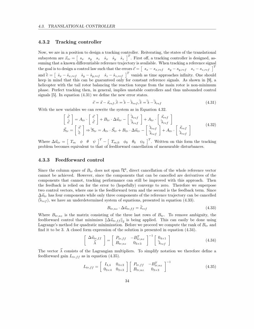
4.3.2 Tracking controller
Now, we are in a position to design a tracking controller. Reiterating, the states of the translationalsubsystem are ~xtr =
[sx sy sz sx sy sz
]T . First off, a tracking controller is designed, as-suming that a known differentiable reference trajectory is available. When tracking a reference signalthe goal is to design a control law such that the errors ~e =
[sx − sx,ref sy − sy,ref sz − sz,ref
]Tand~e =
[sx − sx,ref sy − sy,ref sz − sz,ref
]T vanish as time approaches infinity. One shouldkeep in mind that this can be guaranteed only for constant reference signals. As shown in [9], ahelicopter with the tail rotor balancing the reaction torque from the main rotor is non-minimumphase. Perfect tracking then, in general, implies unstable controllers and thus unbounded controlsignals [5]. In equation (4.31) we define the new error states.
~e = ~s− ~sref ,~e =~s−~sref ,~e =~s−~sref (4.31)
With the new variables we can rewrite the system as in Equation 4.32.[~e
~e
]= Atr ·
[~e
~e
]+Btr ·∆~utr −
[~sref~sref
]+Atr ·
[~sref~sref
]~Str =
[~e
~e
]⇒~Str = Atr · ~Str +Btr ·∆~utr −
[~sref~sref
]+Atr ·
[~sref~sref
] (4.32)
Where ∆~utr =[Tm φ θ ψ
]T − [ Tm,0 φ0 θ0 ψ0
]T . Written on this form the trackingproblem becomes equivalent to that of feedforward cancellation of measurable disturbances.
4.3.3 Feedforward control
Since the column space of Btr does not span R6, direct cancellation of the whole reference vectorcannot be achieved. However, since the components that can be cancelled are derivatives of thecomponents that cannot, tracking performance can still be improved with this approach. Thenthe feedback is relied on for the error to (hopefully) converge to zero. Therefore we superposetwo control vectors, where one is the feedforward term and the second is the feedback term. Since∆~utr has four components while only three components of the reference trajectory can be cancelled(~sref ), we have an underdetermined system of equations, presented in equation (4.33).
Btr,nz ·∆~utr,ff = ~sref (4.33)
Where Btr,nz is the matrix consisting of the three last rows of Btr. To remove ambiguity, thefeedforward control that minimizes ‖∆~utr,ff‖2 is being applied. This can easily be done usingLagrange’s method for quadratic minimization. Before we proceed we compute the rank of Btr andfind it to be 3. A closed form expression of the solution is presented in equation (4.34).[
∆~utr,ff~λ
]=
[Ptr,ff −BTtr,nzBtr,nz 03×3
]−1 [04×1
~sref
](4.34)
The vector ~λ consists of the Lagrangian multipliers. To simplify notation we therefore define afeedforward gain Ltr,ff as in equation (4.35).
Ltr,ff =
[I4,4 04×3
03×4 03×3
] [Ptr,ff −BTtr,nzBtr,nz 03×3
]−1
(4.35)
34
4.3. TRANSLATIONAL CONTROLLER
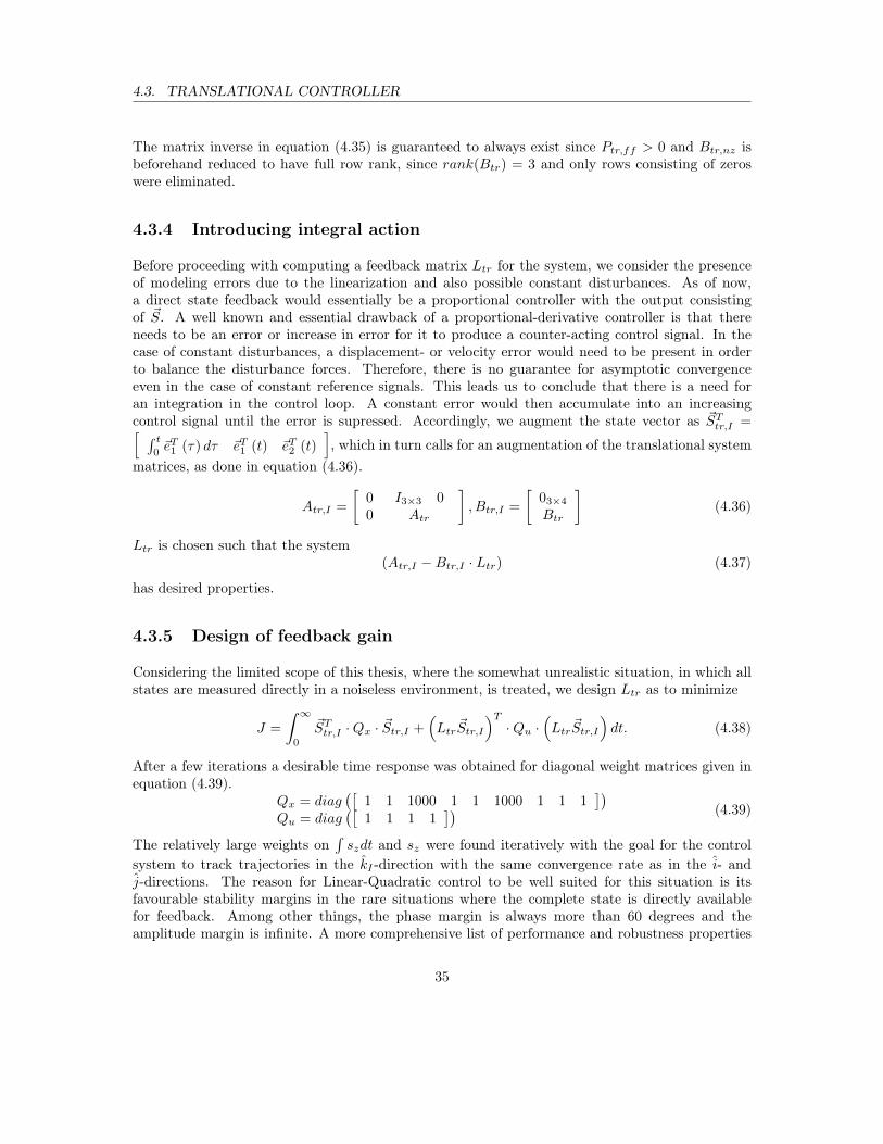
The matrix inverse in equation (4.35) is guaranteed to always exist since Ptr,ff > 0 and Btr,nz isbeforehand reduced to have full row rank, since rank(Btr) = 3 and only rows consisting of zeroswere eliminated.
4.3.4 Introducing integral action
Before proceeding with computing a feedback matrix Ltr for the system, we consider the presenceof modeling errors due to the linearization and also possible constant disturbances. As of now,a direct state feedback would essentially be a proportional controller with the output consistingof ~S. A well known and essential drawback of a proportional-derivative controller is that thereneeds to be an error or increase in error for it to produce a counter-acting control signal. In thecase of constant disturbances, a displacement- or velocity error would need to be present in orderto balance the disturbance forces. Therefore, there is no guarantee for asymptotic convergenceeven in the case of constant reference signals. This leads us to conclude that there is a need foran integration in the control loop. A constant error would then accumulate into an increasingcontrol signal until the error is supressed. Accordingly, we augment the state vector as ~STtr,I =[ ∫ t
0~eT1 (τ) dτ ~eT1 (t) ~eT2 (t)
], which in turn calls for an augmentation of the translational system
matrices, as done in equation (4.36).
Atr,I =
[0 I3×3 00 Atr
], Btr,I =
[03×4
Btr
](4.36)
Ltr is chosen such that the system(Atr,I −Btr,I · Ltr) (4.37)
has desired properties.
4.3.5 Design of feedback gain
Considering the limited scope of this thesis, where the somewhat unrealistic situation, in which allstates are measured directly in a noiseless environment, is treated, we design Ltr as to minimize
J =
∫ ∞0
~STtr,I ·Qx · ~Str,I +(Ltr ~Str,I
)T·Qu ·
(Ltr ~Str,I
)dt. (4.38)
After a few iterations a desirable time response was obtained for diagonal weight matrices given inequation (4.39).
Qx = diag([
1 1 1000 1 1 1000 1 1 1])
Qu = diag([
1 1 1 1]) (4.39)
The relatively large weights on∫szdt and sz were found iteratively with the goal for the control
system to track trajectories in the kI -direction with the same convergence rate as in the i- andj-directions. The reason for Linear-Quadratic control to be well suited for this situation is itsfavourable stability margins in the rare situations where the complete state is directly availablefor feedback. Among other things, the phase margin is always more than 60 degrees and theamplitude margin is infinite. A more comprehensive list of performance and robustness properties
35
4.3. TRANSLATIONAL CONTROLLER
with derivations can be found on p. 289 in [5]. The complete translational control law can then bestated as in equation (4.40)
~utr =[Tm,0 φ0 θ0 ψ0
]T+ Ltr,ff · ~sref − Ltr · ~Str,I (4.40)
The setpoint controller is intentionally overlooked in this section since it is essentially covered by thetracking controller, only by setting the derivatives ~sref , ~sref to zero. Note that this should be doneexplicitly since direct differentiation of a step reference yields a Dirac impulse. For general inputsignals one can apply a lowpass prefilter to the reference signals, since this also would accomodate theuse of reference signals computed in discrete time, essentially making the prefilter a reconstructionfilter.
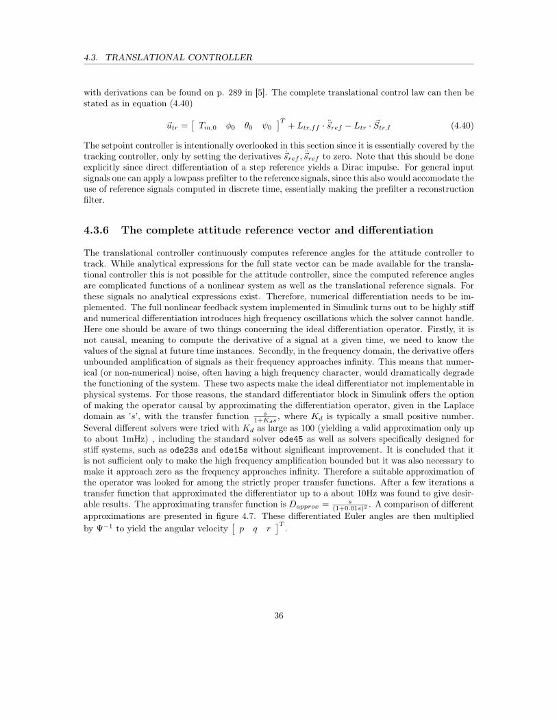
4.3.6 The complete attitude reference vector and differentiation
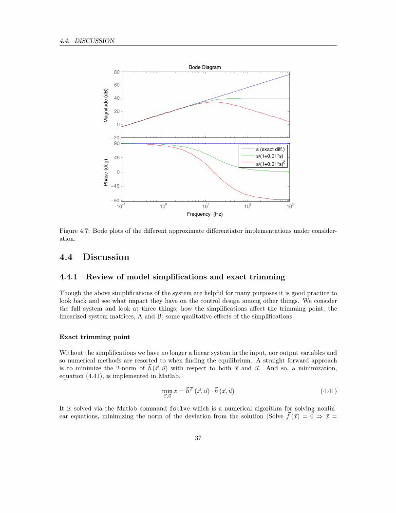
The translational controller continuously computes reference angles for the attitude controller totrack. While analytical expressions for the full state vector can be made available for the transla-tional controller this is not possible for the attitude controller, since the computed reference anglesare complicated functions of a nonlinear system as well as the translational reference signals. Forthese signals no analytical expressions exist. Therefore, numerical differentiation needs to be im-plemented. The full nonlinear feedback system implemented in Simulink turns out to be highly stiffand numerical differentiation introduces high frequency oscillations which the solver cannot handle.Here one should be aware of two things concerning the ideal differentiation operator. Firstly, it isnot causal, meaning to compute the derivative of a signal at a given time, we need to know thevalues of the signal at future time instances. Secondly, in the frequency domain, the derivative offersunbounded amplification of signals as their frequency approaches infinity. This means that numer-ical (or non-numerical) noise, often having a high frequency character, would dramatically degradethe functioning of the system. These two aspects make the ideal differentiator not implementable inphysical systems. For those reasons, the standard differentiator block in Simulink offers the optionof making the operator causal by approximating the differentiation operator, given in the Laplacedomain as ’s’, with the transfer function s
1+Kds, where Kd is typically a small positive number.
Several different solvers were tried with Kd as large as 100 (yielding a valid approximation only upto about 1mHz) , including the standard solver ode45 as well as solvers specifically designed forstiff systems, such as ode23s and ode15s without significant improvement. It is concluded that itis not sufficient only to make the high frequency amplification bounded but it was also necessary tomake it approach zero as the frequency approaches infinity. Therefore a suitable approximation ofthe operator was looked for among the strictly proper transfer functions. After a few iterations atransfer function that approximated the differentiator up to a about 10Hz was found to give desir-able results. The approximating transfer function is Dapprox = s
(1+0.01s)2 . A comparison of differentapproximations are presented in figure 4.7. These differentiated Euler angles are then multipliedby Ψ−1 to yield the angular velocity
[p q r
]T .
36
4.4. DISCUSSION
!"
"
!"
#"
$"
%"
&'()*+,-./0-12
3" 3 3"" 3"3 3"! 3"45"
#6
"
#6
5"
78'9./0-.(2
/
/
1:-./;*'(<'=
><.?,.)@A//0BC2
9/0.D'@+/-*EEF29G03H"F"3I92
9G03H"F"3I92!
Figure 4.7: Bode plots of the different approximate differentiator implementations under consider-ation.
4.4 Discussion
4.4.1 Review of model simplifications and exact trimming
Though the above simplifications of the system are helpful for many purposes it is good practice tolook back and see what impact they have on the control design among other things. We considerthe full system and look at three things; how the simplifications affect the trimming point; thelinearized system matrices, A and B; some qualitative effects of the simplifications.
Exact trimming point
Without the simplifications we have no longer a linear system in the input, nor output variables andso numerical methods are resorted to when finding the equilibrium. A straight forward approachis to minimize the 2-norm of ~h (~x, ~u) with respect to both ~x and ~u. And so, a minimization,equation (4.41), is implemented in Matlab.
min~x,~u
z = ~hT (~x, ~u) · ~h (~x, ~u) (4.41)
It is solved via the Matlab command fsolve which is a numerical algorithm for solving nonlin-ear equations, minimizing the norm of the deviation from the solution (Solve ~f (~x) = ~0 ⇒ ~x =
37
4.4. DISCUSSION
arg min ~f (~x)T · ~f (~x)). The input ~u0 for which at least one equilibrium of the system exists is
presented in equation (4.42).
~uT0 =[a0 b0 Tm,0 Tt,0
]=[−0.000257 0.00475 80.4 4.22
](4.42)
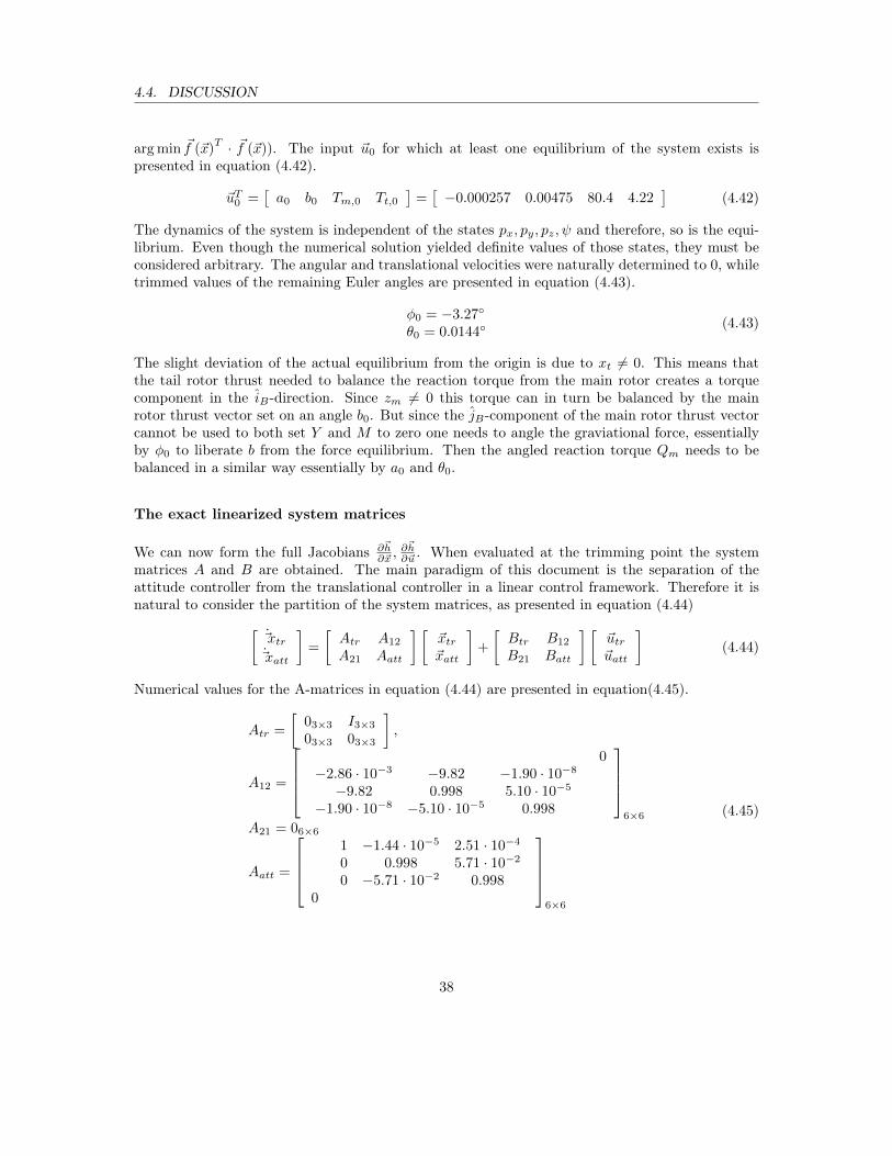
The dynamics of the system is independent of the states px, py, pz, ψ and therefore, so is the equi-librium. Even though the numerical solution yielded definite values of those states, they must beconsidered arbitrary. The angular and translational velocities were naturally determined to 0, whiletrimmed values of the remaining Euler angles are presented in equation (4.43).
φ0 = −3.27◦
θ0 = 0.0144◦(4.43)
The slight deviation of the actual equilibrium from the origin is due to xt 6= 0. This means thatthe tail rotor thrust needed to balance the reaction torque from the main rotor creates a torquecomponent in the iB-direction. Since zm 6= 0 this torque can in turn be balanced by the mainrotor thrust vector set on an angle b0. But since the jB-component of the main rotor thrust vectorcannot be used to both set Y and M to zero one needs to angle the graviational force, essentiallyby φ0 to liberate b from the force equilibrium. Then the angled reaction torque Qm needs to bebalanced in a similar way essentially by a0 and θ0.
The exact linearized system matrices
We can now form the full Jacobians ∂~h∂~x ,
∂~h∂~u . When evaluated at the trimming point the system
matrices A and B are obtained. The main paradigm of this document is the separation of theattitude controller from the translational controller in a linear control framework. Therefore it isnatural to consider the partition of the system matrices, as presented in equation (4.44)[
~xtr~xatt
]=
[Atr A12
A21 Aatt
] [~xtr~xatt
]+
[Btr B12
B21 Batt
] [~utr~uatt
](4.44)
Numerical values for the A-matrices in equation (4.44) are presented in equation(4.45).
Atr =
[03×3 I3×3
03×3 03×3
],
A12 =
0
−2.86 · 10−3 −9.82 −1.90 · 10−8
−9.82 0.998 5.10 · 10−5
−1.90 · 10−8 −5.10 · 10−5 0.998
6×6
A21 = 06×6
Aatt =
1 −1.44 · 10−5 2.51 · 10−4
0 0.998 5.71 · 10−2
0 −5.71 · 10−2 0.9980
6×6
(4.45)
38
4.4. DISCUSSION
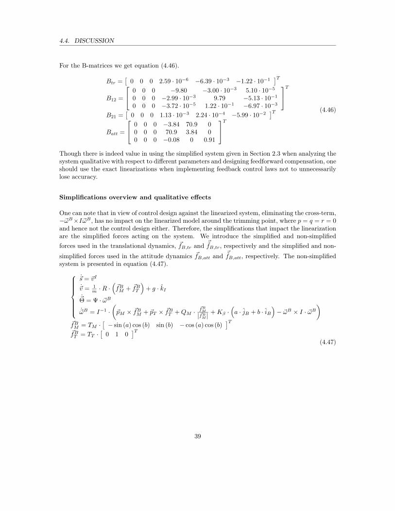
For the B-matrices we get equation (4.46).
Btr =[
0 0 0 2.59 · 10−6 −6.39 · 10−3 −1.22 · 10−1]T
B12 =
0 0 0 −9.80 −3.00 · 10−3 5.10 · 10−5
0 0 0 −2.99 · 10−3 9.79 −5.13 · 10−1
0 0 0 −3.72 · 10−5 1.22 · 10−1 −6.97 · 10−3
TB21 =
[0 0 0 1.13 · 10−3 2.24 · 10−4 −5.99 · 10−2
]TBatt =
0 0 0 −3.84 70.9 00 0 0 70.9 3.84 00 0 0 −0.08 0 0.91
T(4.46)
Though there is indeed value in using the simplified system given in Section 2.3 when analyzing thesystem qualitative with respect to different parameters and designing feedforward compensation, oneshould use the exact linearizations when implementing feedback control laws not to unnecessarilylose accuracy.
Simplifications overview and qualitative effects
One can note that in view of control design against the linearized system, eliminating the cross-term,−~ωB×I~ωB , has no impact on the linearized model around the trimming point, where p = q = r = 0and hence not the control design either. Therefore, the simplifications that impact the linearizationare the simplified forces acting on the system. We introduce the simplified and non-simplifiedforces used in the translational dynamics, ~fB,tr and ~
fB,tr, respectively and the simplified and non-
simplified forces used in the attitude dynamics ~fB,att and~fB,att, respectively. The non-simplified
system is presented in equation (4.47).
~s = ~vI
~v = 1m ·R ·
(~fBM + ~fBT
)+ g · kI
~Θ = Ψ · ~ωB
~ωB = I−1 ·(~pM × ~fBM + ~pT × ~fBT +QM ·
~fBM
|~fBM |+Kβ ·
(a · jB + b · iB
)− ~ωB × I · ~ωB
)~fBM = TM ·
[− sin (a) cos (b) sin (b) − cos (a) cos (b)
]T~fBT = TT ·
[0 1 0
]T(4.47)
39
4.4. DISCUSSION
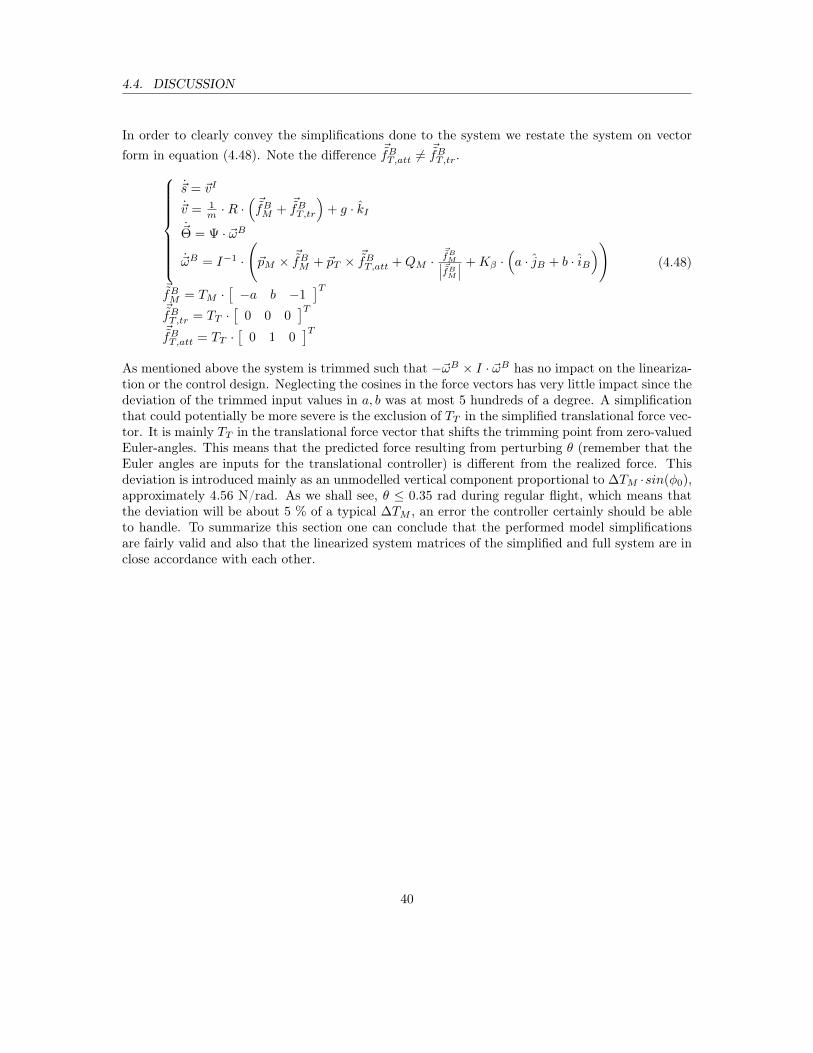
In order to clearly convey the simplifications done to the system we restate the system on vectorform in equation (4.48). Note the difference ~fBT,att 6=
~fBT,tr.
~s = ~vI
~v = 1m ·R ·
(~fBM +
~fBT,tr
)+ g · kI
~Θ = Ψ · ~ωB
~ωB = I−1 ·
(~pM × ~
fBM + ~pT × ~fBT,att +QM ·
~fBM∣∣∣ ~fBM ∣∣∣ +Kβ ·
(a · jB + b · iB
))~fBM = TM ·
[−a b −1
]T~fBT,tr = TT ·
[0 0 0
]T~fBT,att = TT ·
[0 1 0
]T
(4.48)
As mentioned above the system is trimmed such that −~ωB × I · ~ωB has no impact on the lineariza-tion or the control design. Neglecting the cosines in the force vectors has very little impact since thedeviation of the trimmed input values in a, b was at most 5 hundreds of a degree. A simplificationthat could potentially be more severe is the exclusion of TT in the simplified translational force vec-tor. It is mainly TT in the translational force vector that shifts the trimming point from zero-valuedEuler-angles. This means that the predicted force resulting from perturbing θ (remember that theEuler angles are inputs for the translational controller) is different from the realized force. Thisdeviation is introduced mainly as an unmodelled vertical component proportional to ∆TM ·sin(φ0),approximately 4.56 N/rad. As we shall see, θ ≤ 0.35 rad during regular flight, which means thatthe deviation will be about 5 % of a typical ∆TM , an error the controller certainly should be ableto handle. To summarize this section one can conclude that the performed model simplificationsare fairly valid and also that the linearized system matrices of the simplified and full system are inclose accordance with each other.
40
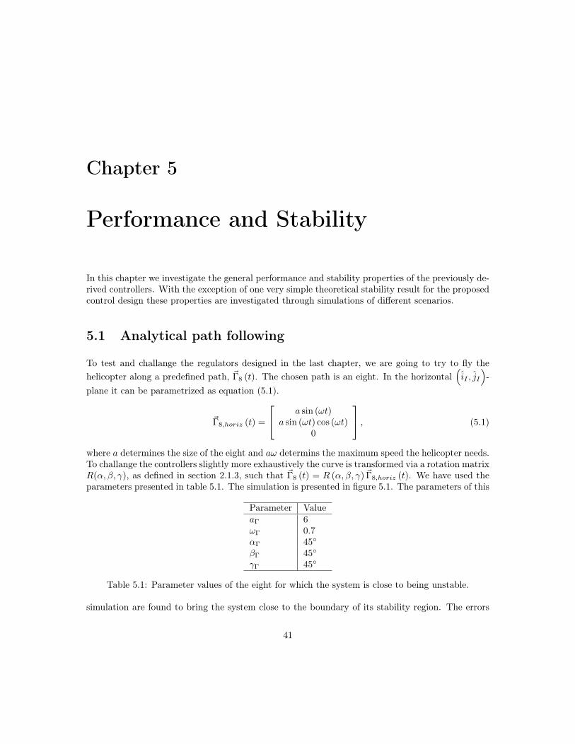
Chapter 5
Performance and Stability
In this chapter we investigate the general performance and stability properties of the previously de-rived controllers. With the exception of one very simple theoretical stability result for the proposedcontrol design these properties are investigated through simulations of different scenarios.
5.1 Analytical path following
To test and challange the regulators designed in the last chapter, we are going to try to fly thehelicopter along a predefined path, ~Γ8 (t). The chosen path is an eight. In the horizontal
(iI , jI
)-
plane it can be parametrized as equation (5.1).
~Γ8,horiz (t) =
a sin (ωt)a sin (ωt) cos (ωt)
0
, (5.1)
where a determines the size of the eight and aω determins the maximum speed the helicopter needs.To challange the controllers slightly more exhaustively the curve is transformed via a rotation matrixR(α, β, γ), as defined in section 2.1.3, such that ~Γ8 (t) = R (α, β, γ) ~Γ8,horiz (t). We have used theparameters presented in table 5.1. The simulation is presented in figure 5.1. The parameters of this
Parameter ValueaΓ 6ωΓ 0.7αΓ 45◦
βΓ 45◦
γΓ 45◦
Table 5.1: Parameter values of the eight for which the system is close to being unstable.
simulation are found to bring the system close to the boundary of its stability region. The errors
41
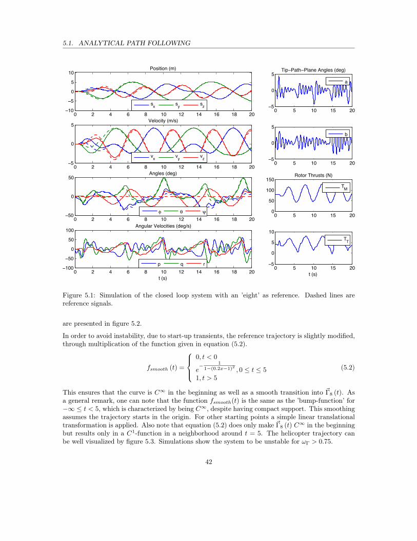
5.1. ANALYTICAL PATH FOLLOWING
! " # $ % &! &" &# &$ &% "!&!
'
!
'
&!()*+,+)-./01
.
.
*2 *3 *4! ' &! &' "!'
!
'5+6 (7,8 (97-:.;-<9:*./=:<1
.
.7
! " # $ % &! &" &# &$ &% "!'
!
'>:9)?+,3./0@*1
.
.
A2 A3 A4! ' &! &' "!'
!
'
.
.B
! " # $ % &! &" &# &$ &% "!'!
!
'!;-<9:*./=:<1
.
.
! ' &! &' "!!
'!
&!!
&'!C),)D.58DE*,*./F1
.
.5G
! " # $ % &! &" &# &$ &% "!&!!
'!
!
'!
&!!
,./*1
;-<E97D.>:9)?+,+:*./=:<@*1
.
.
6 H D! ' &! &' "!'
!
'
&!
,./*1
.
.55
Figure 5.1: Simulation of the closed loop system with an ’eight’ as reference. Dashed lines arereference signals.
are presented in figure 5.2.
In order to avoid instability, due to start-up transients, the reference trajectory is slightly modified,through multiplication of the function given in equation (5.2).
fsmooth (t) =
0, t < 0
e− 1
1−(0.2x−1)2 , 0 ≤ t ≤ 51, t > 5
(5.2)
This ensures that the curve is C∞ in the beginning as well as a smooth transition into ~Γ8 (t). Asa general remark, one can note that the function fsmooth(t) is the same as the ’bump-function’ for−∞ ≤ t < 5, which is characterized by being C∞, despite having compact support. This smoothingassumes the trajectory starts in the origin. For other starting points a simple linear translationaltransformation is applied. Also note that equation (5.2) does only make ~Γ8 (t) C∞ in the beginningbut results only in a C1-function in a neighborhood around t = 5. The helicopter trajectory canbe well visualized by figure 5.3. Simulations show the system to be unstable for ωΓ > 0.75.
42
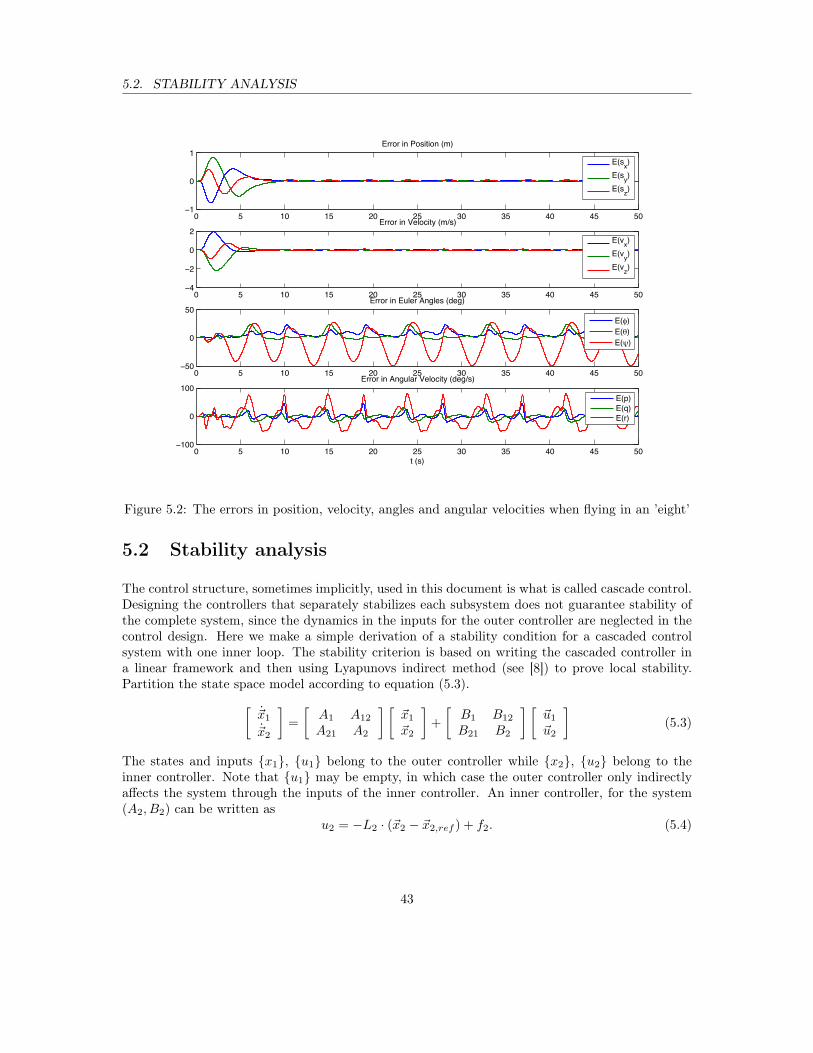
5.2. STABILITY ANALYSIS
0 5 10 15 20 25 30 35 40 45 501
0
1Error in Position (m)
E(sx)E(sy)E(sz)
0 5 10 15 20 25 30 35 40 45 504
2
0
2Error in Velocity (m/s)
E(vx)E(vy)E(vz)
0 5 10 15 20 25 30 35 40 45 5050
0
50Error in Euler Angles (deg)
E( )E( )E( )
0 5 10 15 20 25 30 35 40 45 50100
0
100
t (s)
Error in Angular Velocity (deg/s)
E(p)E(q)E(r)
Figure 5.2: The errors in position, velocity, angles and angular velocities when flying in an ’eight’
5.2 Stability analysis
The control structure, sometimes implicitly, used in this document is what is called cascade control.Designing the controllers that separately stabilizes each subsystem does not guarantee stability ofthe complete system, since the dynamics in the inputs for the outer controller are neglected in thecontrol design. Here we make a simple derivation of a stability condition for a cascaded controlsystem with one inner loop. The stability criterion is based on writing the cascaded controller ina linear framework and then using Lyapunovs indirect method (see [8]) to prove local stability.Partition the state space model according to equation (5.3).[
~x1
~x2
]=
[A1 A12
A21 A2
] [~x1
~x2
]+
[B1 B12
B21 B2
] [~u1
~u2
](5.3)
The states and inputs {x1}, {u1} belong to the outer controller while {x2}, {u2} belong to theinner controller. Note that {u1} may be empty, in which case the outer controller only indirectlyaffects the system through the inputs of the inner controller. An inner controller, for the system(A2, B2) can be written as
u2 = −L2 · (~x2 − ~x2,ref ) + f2. (5.4)
43
5.2. STABILITY ANALYSIS
Figure 5.3: 3D visualization of the system simulated while following the eight-shaped reference withparameter values given in table 5.1
Then, we design an outer controller for the system(A1,
[B1 A12
])as[
~u1
~x2,ref
]= −
[L11
L12
]· (x1 − x1,ref ) +
[f11
f12
]. (5.5)
Introducing the errors ~ei = ~xi − ~xi,ref and substituting equations (5.4), (5.5) into equation (5.3),we obtain equation (5.6).[
~e1
~e2
]= H−1
({A ·H −B ·
[L11 00 L2
]}·[~e1
~e2
]+B ·
[~f11
~f2
]+A ·
[~x1,r
~f12
]−
[~x1,r
~f12
]),
(5.6)
44
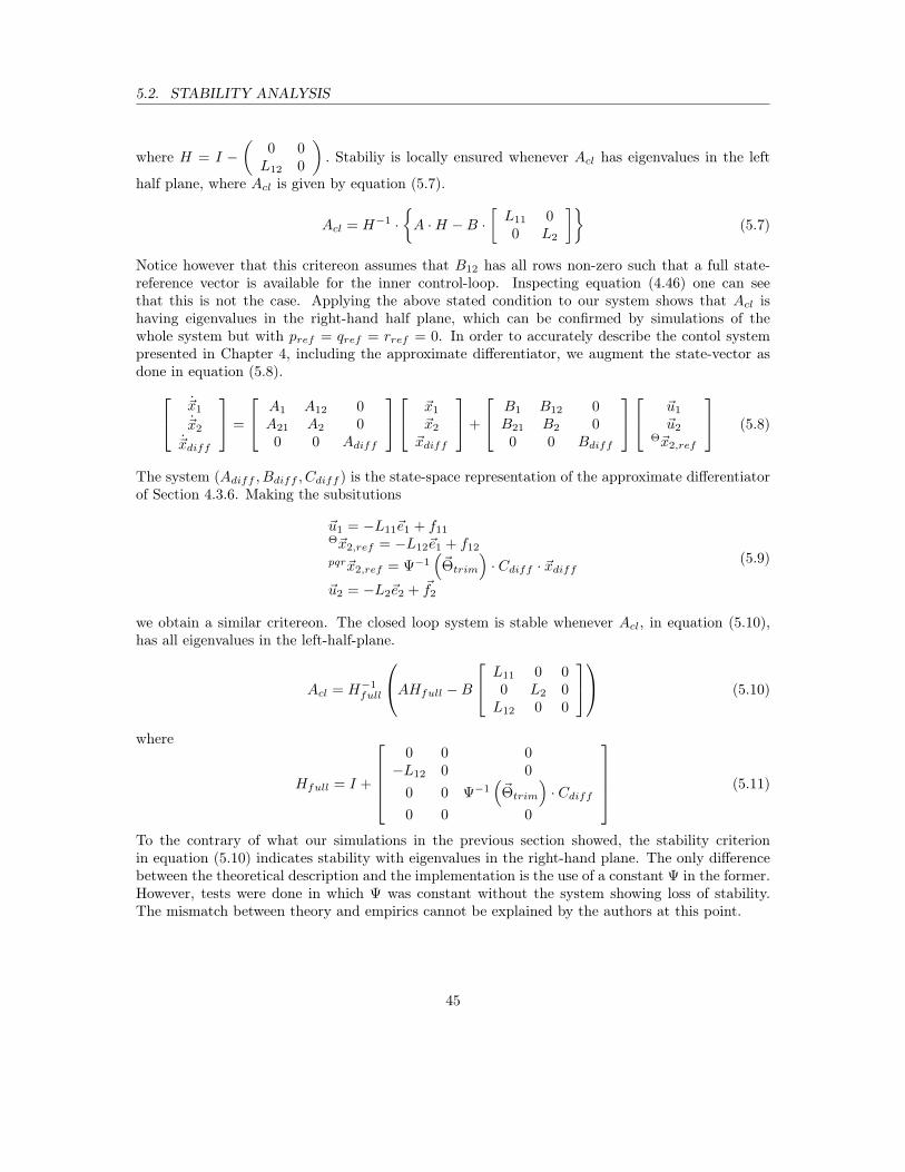
5.2. STABILITY ANALYSIS
where H = I −(
0 0L12 0
). Stabiliy is locally ensured whenever Acl has eigenvalues in the left
half plane, where Acl is given by equation (5.7).
Acl = H−1 ·{A ·H −B ·
[L11 00 L2
]}(5.7)
Notice however that this critereon assumes that B12 has all rows non-zero such that a full state-reference vector is available for the inner control-loop. Inspecting equation (4.46) one can seethat this is not the case. Applying the above stated condition to our system shows that Acl ishaving eigenvalues in the right-hand half plane, which can be confirmed by simulations of thewhole system but with pref = qref = rref = 0. In order to accurately describe the contol systempresented in Chapter 4, including the approximate differentiator, we augment the state-vector asdone in equation (5.8). ~x1
~x2
~xdiff
=
A1 A12 0A21 A2 00 0 Adiff
~x1
~x2
~xdiff
+
B1 B12 0B21 B2 00 0 Bdiff
~u1
~u2Θ~x2,ref
(5.8)
The system (Adiff , Bdiff , Cdiff ) is the state-space representation of the approximate differentiatorof Section 4.3.6. Making the subsitutions
~u1 = −L11~e1 + f11Θ~x2,ref = −L12~e1 + f12
pqr~x2,ref = Ψ−1(~Θtrim
)· Cdiff · ~xdiff
~u2 = −L2~e2 + ~f2
(5.9)
we obtain a similar critereon. The closed loop system is stable whenever Acl, in equation (5.10),has all eigenvalues in the left-half-plane.
Acl = H−1full
AHfull −B
L11 0 00 L2 0L12 0 0
(5.10)
where
Hfull = I +
0 0 0−L12 0 0
0 0 Ψ−1(~Θtrim
)· Cdiff
0 0 0
(5.11)
To the contrary of what our simulations in the previous section showed, the stability criterionin equation (5.10) indicates stability with eigenvalues in the right-hand plane. The only differencebetween the theoretical description and the implementation is the use of a constant Ψ in the former.However, tests were done in which Ψ was constant without the system showing loss of stability.The mismatch between theory and empirics cannot be explained by the authors at this point.
45
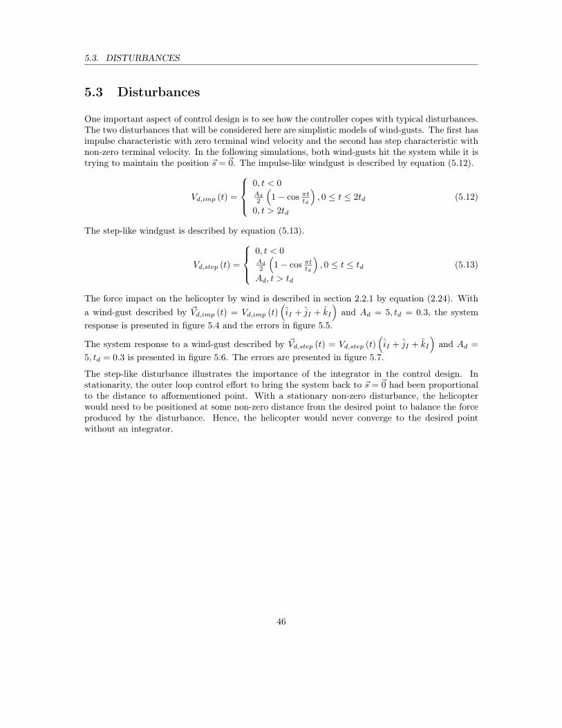
5.3. DISTURBANCES
5.3 Disturbances
One important aspect of control design is to see how the controller copes with typical disturbances.The two disturbances that will be considered here are simplistic models of wind-gusts. The first hasimpulse characteristic with zero terminal wind velocity and the second has step characteristic withnon-zero terminal velocity. In the following simulations, both wind-gusts hit the system while it istrying to maintain the position ~s = ~0. The impulse-like windgust is described by equation (5.12).
Vd,imp (t) =
0, t < 0Ad2
(1− cos πttd
), 0 ≤ t ≤ 2td
0, t > 2td
(5.12)
The step-like windgust is described by equation (5.13).
Vd,step (t) =
0, t < 0Ad2
(1− cos πttd
), 0 ≤ t ≤ td
Ad, t > td
(5.13)
The force impact on the helicopter by wind is described in section 2.2.1 by equation (2.24). Witha wind-gust described by ~Vd,imp (t) = Vd,imp (t)
(iI + jI + kI
)and Ad = 5, td = 0.3, the system
response is presented in figure 5.4 and the errors in figure 5.5.
The system response to a wind-gust described by ~Vd,step (t) = Vd,step (t)(iI + jI + kI
)and Ad =
5, td = 0.3 is presented in figure 5.6. The errors are presented in figure 5.7.
The step-like disturbance illustrates the importance of the integrator in the control design. Instationarity, the outer loop control effort to bring the system back to ~s = ~0 had been proportionalto the distance to afformentioned point. With a stationary non-zero disturbance, the helicopterwould need to be positioned at some non-zero distance from the desired point to balance the forceproduced by the disturbance. Hence, the helicopter would never converge to the desired pointwithout an integrator.
46
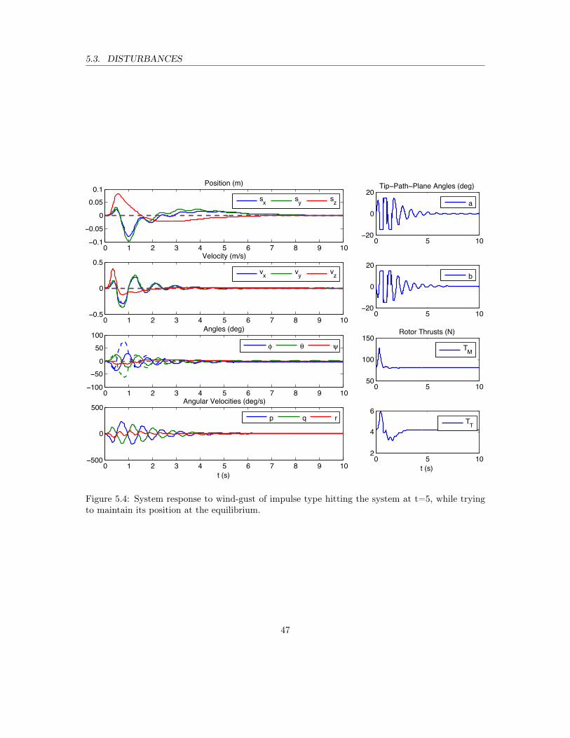
5.3. DISTURBANCES
0 1 2 3 4 5 6 7 8 9 10−0.1
−0.05
0
0.050.1
Position (m)
sx sy sz
0 5 10−20
0
20Tip−Path−Plane Angles (deg)
a
0 1 2 3 4 5 6 7 8 9 10−0.5
0
0.5Velocity (m/s)
vx vy vz
0 5 10−20
0
20
b
0 1 2 3 4 5 6 7 8 9 10−100
−500
50100
Angles (deg)
! " #
0 5 1050
100
150Rotor Thrusts (N)
TM
0 1 2 3 4 5 6 7 8 9 10−500
0
500
t (s)
Angular Velocities (deg/s)
p q r
0 5 102
4
6
t (s)
TT
Figure 5.4: System response to wind-gust of impulse type hitting the system at t=5, while tryingto maintain its position at the equilibrium.
47
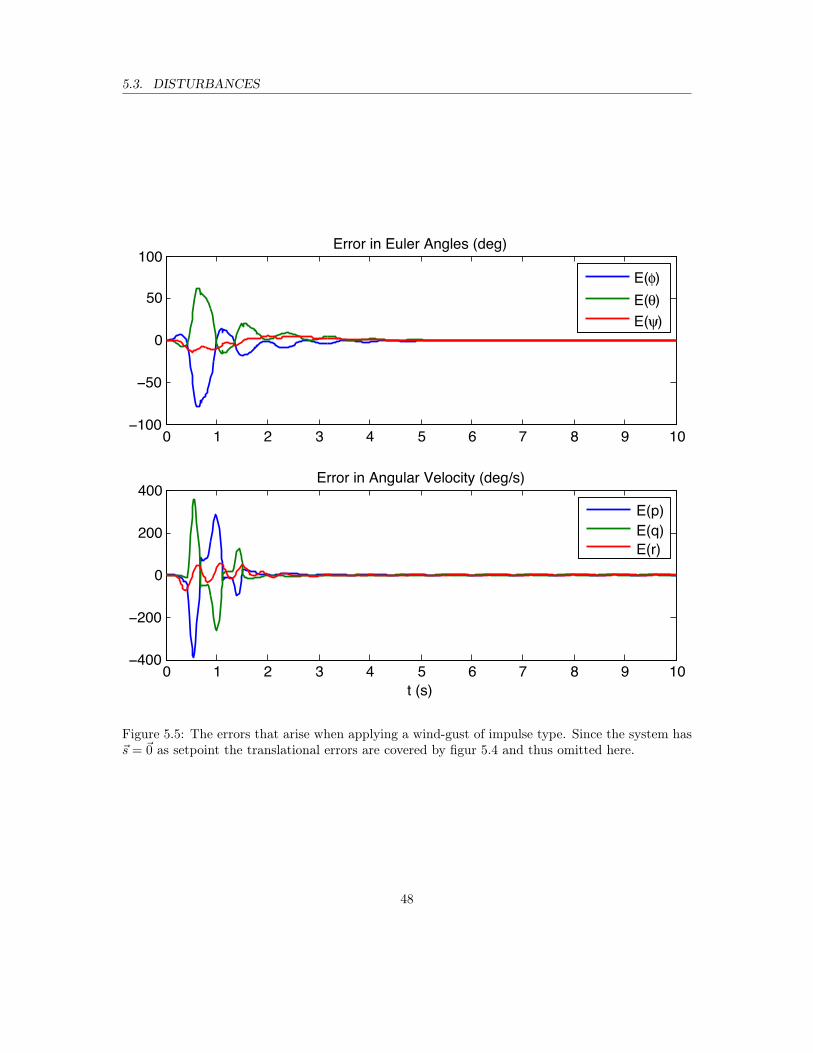
5.3. DISTURBANCES
0 1 2 3 4 5 6 7 8 9 10−100
−50
0
50
100Error in Euler Angles (deg)
E(!)E(")E(#)
0 1 2 3 4 5 6 7 8 9 10−400
−200
0
200
400
t (s)
Error in Angular Velocity (deg/s)
E(p)E(q)E(r)
Figure 5.5: The errors that arise when applying a wind-gust of impulse type. Since the system has~s = ~0 as setpoint the translational errors are covered by figur 5.4 and thus omitted here.
48
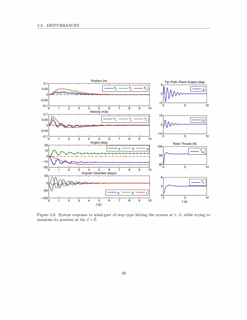
5.3. DISTURBANCES
0 1 2 3 4 5 6 7 8 9 10−0.1
−0.05
0
0.050.1
Position (m)
sx sy sz
0 5 10−5
0
5Tip−Path−Plane Angles (deg)
a
0 1 2 3 4 5 6 7 8 9 10−0.1
−0.050
0.050.1
Velocity (m/s)
vx vy vz
0 5 10−10
0
10
b
0 1 2 3 4 5 6 7 8 9 10−20
−100
1020
Angles (deg)
! " #
0 5 1080
90
100Rotor Thrusts (N)
TM
0 1 2 3 4 5 6 7 8 9 10−100
−50
0
50
t (s)
Angular Velocities (deg/s)
p q r0 5 10
4
5
6
t (s)
TT
Figure 5.6: System response to wind-gust of step type hitting the system at t=5, while trying tomaintain its position at the ~s = ~0.
49
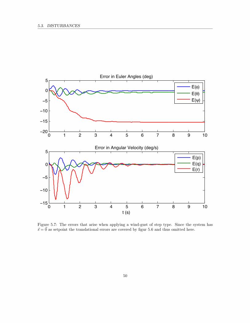
5.3. DISTURBANCES
0 1 2 3 4 5 6 7 8 9 10−20
−15
−10
−5
0
5Error in Euler Angles (deg)
E(!)E(")E(#)
0 1 2 3 4 5 6 7 8 9 10−15
−10
−5
0
5
t (s)
Error in Angular Velocity (deg/s)
E(p)E(q)E(r)
Figure 5.7: The errors that arise when applying a wind-gust of step type. Since the system has~s = ~0 as setpoint the translational errors are covered by figur 5.6 and thus omitted here.
50
Chapter 6
Landing Scenario
Having designed and verified a controller for the helicopter we are now in a position to attack thecore problem of the essay: landing the helicopter on a mobile platform. We start out with definingwhat simplifying premises govern the landing.
6.1 Landing premises
Typical mobile platforms that could come into consideration include the deck of a ship or theflatbed of a truck. Apart from the steady cruising, the motion of a ship can be characterized bythe periodic rocking due to surrounding waves. Methods for predictions of ship motion has beenpresented in [16] with high accuracy with at least four seconds prediction horizons. This leads to thepremise that the ship motion is known at least four seconds into the future. Also, it is reasonableto assume that flying a helicopter is avoided under severe weather conditions which allows us tolimit the amplitudes of the ship motion to a small value. Therefore we, somewhat arbitrarily, limitthe amplitude to half a meter in each direction. The dynamics of the used model for the helicopterdoes not contain ~s and is therefore invariant under Galileo transformations. Thus, the steadycruising does not need to be included in description of the platform motion. Therefore, one can seeequation (6.1) as the deviations from the steady cruising motion. In practice, this motion would bea non-analytical output from some kind of prediction filter so in order to simplify the exposition ofthis chapter we describe the predicted trajectory by a set of simple sinusoids, including the attitudeof the platform, as can be seen in equation (6.1)
~spf (t) =
15 sin (t−∆tpf )sin (t−∆tpf )
14 sin (t−∆tpf )
, ~Θpf (t) =
14 sin (t−∆tpf )12 sin (t−∆tpf )15 sin (t−∆tpf )
(6.1)
The position of the platform is denoted by ~spf and ~Θpf denotes the attitude of the platform, in thesame set of Euler angles describing the attitude of the helicopter. Lastly, we define what constitutesa successful landing. Ideally, the relative velocity between the platform and the helicopter wouldbe zero at touchdown, but due to several imperfections such as model approximations (the main
51
6.2. TRAJECTORY GENERATION
reason in the simulations due to the linear trajectory planning) and disturbances (an importantfactor during a real life landing), this is close to impossible. For a successful landing to take place,we say that the relative speed parallel to the platform at impact must be less than 0.4 m/s and thenormal speed less than 0.47 m/s. Since we do not have access to the geometry of the helicopterin relation to its center of gravity it is hard to estimate what lateral velocities (with requiredretardation) are allowed for the helicopter not to overturn. We simply set it to the same orderof magnitude as the allowed normal impact velocity. The angle between the iB , jB-plane and theplatform should not exceed 10 degrees, not to allow the tail-rotor to hit the platform at touchdown.The allowed normal velocity difference corresponds to a free fall from 0.01 m. We estimate that alight model helicopter is able to withstand such small impacts. The positional error at touchdownmay not exceed 0.2 meters for a reasonably sized platform. In addition to these requirements wehave that the helicopter cannot cross the boundary describing the platform at any time during itsflight. For simplicity the platform is considered to be an infinite plane described by a time-varyingcoordinate, ~spf , and three Euler angles, ~Θpf .
6.2 Trajectory generation
There are several reasons why set point control is not feasible during the task of taking a systemfrom ~x0 to ~xf in the state space. For example, if the distance between the two points in thestate space is large, the inputs to the system may take on too large values, either for the system togenerate, withstand or to remain in the linear region for which the linear control law is designed. Theresult may be damaged actuators, sensors and/or instability. Therefore, when achieving the task ofmoving between the two points, an important part is the trajectory generation or path planning,which preferably traces out a smooth curve in the state space, which remains feasible with respectto the system dynamics and without straining the system. Since the control laws, designed inchapter 4, are based on linearization and the assumption that the system is to remain within thelinear region throughout its trajectory, it is reasonable to also generate the trajectory with respectto the linearized system. This can be achieved by a method known as Model Predictive Control(MPC). An introductory description of MPC is given in the next section. Note that throughoutthis section, the equations will sometimes be expressed in terms of ∆~x,∆~u and sometimes in termsof ~x, ~u, according to what is the most convenient. The two versions are never used interchangablythough.
6.2.1 Introduction to model predictive control (MPC)
Given a system , ~x = f (~x, ~u), with nx states and nu input signals, Taylor expansion around~xtrim, ~utrim yields
~x∣∣∣~x=~xtrim~u=~utrim
≈ ~f (~xtrim, ~utrim) = ∂ ~f(~x,~u)∂~x
∣∣∣~x=~xtrim~u=~utrim
· (~x− ~xtrim) + ∂ ~f(~x,~u)∂~u
∣∣∣~x=~xtrim~u=~utrim
· (~u− ~utrim)
⇔ ∆~x ≈ ~f (~xtrim, ~utrim) +A∆~x+B∆~u(6.2)
52
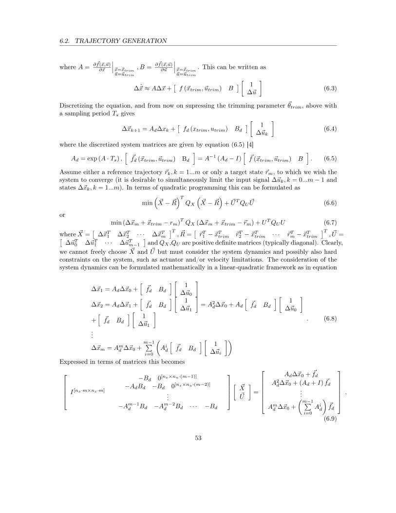
6.2. TRAJECTORY GENERATION
where A = ∂ ~f(~x,~u)∂~x
∣∣∣~x=~xtrim~u=~utrim
, B = ∂ ~f(~x,~u)∂~u
∣∣∣~x=~xtrim~u=~utrim
. This can be written as
∆~x ≈ A∆~x+[f (~xtrim, ~utrim) B
] [ 1∆~u
](6.3)
Discretizing the equation, and from now on supressing the trimming parameter ~θtrim, above witha sampling period Ts gives
∆~xk+1 = Ad∆xk +[fd (xtrim, utrim) Bd
] [ 1∆~uk
](6.4)
where the discretized system matrices are given by equation (6.5) [4]
Ad = exp (A · Ts) ,[~fd (~xtrim, ~utrim) Bd
]= A−1 (Ad − I)
[~f (~xtrim, ~utrim) B
]. (6.5)
Assume either a reference trajectory ~rk, k = 1...m or only a target state ~rm, to which we wish thesystem to converge (it is desirable to simultaneously limit the input signal ∆~uk, k = 0...m− 1 andstates ∆~xk, k = 1...m). In terms of quadratic programming this can be formulated as
min(~X − ~R
)TQX
(~X − ~R
)+ ~UTQU ~U (6.6)
ormin (∆~xm + ~xtrim − rm)
TQX (∆~xm + ~xtrim − ~rm) + UTQUU (6.7)
where ~X =[
∆~xT1 ∆~xT2 · · · ∆~xTm]T, ~R =
[~rT1 − ~xTtrim ~rT2 − ~xTtrim · · · ~rTm − ~xTtrim
]T, ~U =[
∆~uT0 ∆~uT1 · · · ∆~uTm−1
]andQX ,QU are positive definite matrices (typically diagonal). Clearly,
we cannot freely choose ~X and ~U but must consider the system dynamics and possibly also hardconstraints on the system, such as actuator and/or velocity limitations. The consideration of thesystem dynamics can be formulated mathematically in a linear-quadratic framework as in equation
∆~x1 = Ad∆~x0 +[~fd Bd
] [ 1∆~u0
]∆~x2 = Ad∆~x1 +
[~fd Bd
] [1
∆~u1
]= A2
d∆~x0 +Ad
[~fd Bd
] [1
∆~u0
]+[~fd Bd
] [ 1∆~u1
]...
∆~xm = Amd ∆~x0 +m−1∑i=0
(Aid
[~fd Bd
] [1
∆~ui
]). (6.8)
Expressed in terms of matrices this becomes I [nx·m×nx·m]
−Bd 0[nx×nu·(m−1)]
−AdBd −Bd 0[nx×nu·(m−2)]
...−Am−1
d Bd −Am−2d Bd · · · −Bd
[~X~U
]=
Ad∆~x0 + ~fd
A2d∆~x0 + (Ad + I) ~fd
...
Amd ∆~x0 +
(m−1∑i=0
Aid
)~fd
.
(6.9)
53
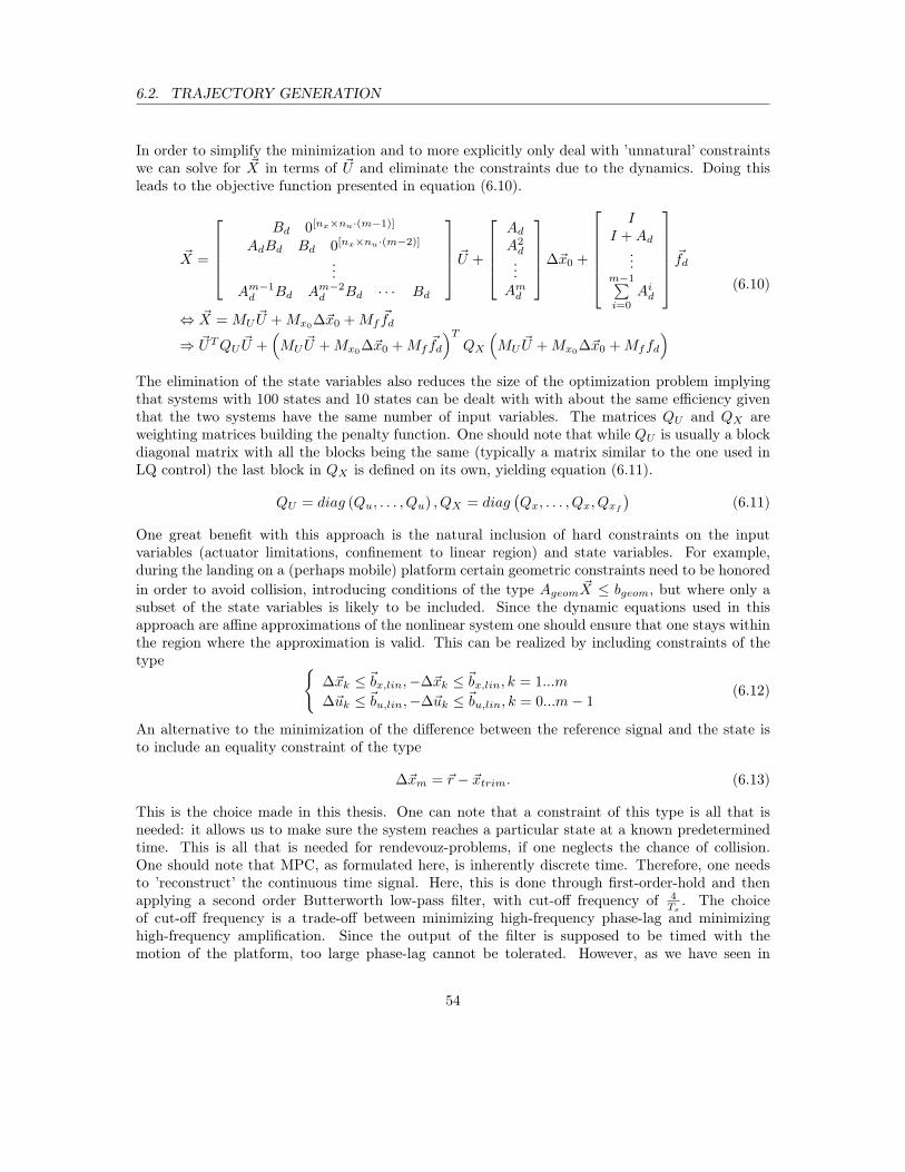
6.2. TRAJECTORY GENERATION
In order to simplify the minimization and to more explicitly only deal with ’unnatural’ constraintswe can solve for ~X in terms of ~U and eliminate the constraints due to the dynamics. Doing thisleads to the objective function presented in equation (6.10).
~X =
Bd 0[nx×nu·(m−1)]
AdBd Bd 0[nx×nu·(m−2)]
...Am−1d Bd Am−2
d Bd · · · Bd
~U +
AdA2d...Amd
∆~x0 +
I
I +Ad...
m−1∑i=0
Aid
~fd⇔ ~X = MU
~U +Mx0∆~x0 +Mf~fd
⇒ ~UTQU ~U +(MU
~U +Mx0∆~x0 +Mf
~fd
)TQX
(MU
~U +Mx0∆~x0 +Mffd
)(6.10)
The elimination of the state variables also reduces the size of the optimization problem implyingthat systems with 100 states and 10 states can be dealt with with about the same efficiency giventhat the two systems have the same number of input variables. The matrices QU and QX areweighting matrices building the penalty function. One should note that while QU is usually a blockdiagonal matrix with all the blocks being the same (typically a matrix similar to the one used inLQ control) the last block in QX is defined on its own, yielding equation (6.11).
QU = diag (Qu, . . . , Qu) , QX = diag(Qx, . . . , Qx, Qxf
)(6.11)
One great benefit with this approach is the natural inclusion of hard constraints on the inputvariables (actuator limitations, confinement to linear region) and state variables. For example,during the landing on a (perhaps mobile) platform certain geometric constraints need to be honoredin order to avoid collision, introducing conditions of the type Ageom ~X ≤ bgeom, but where only asubset of the state variables is likely to be included. Since the dynamic equations used in thisapproach are affine approximations of the nonlinear system one should ensure that one stays withinthe region where the approximation is valid. This can be realized by including constraints of thetype {
∆~xk ≤ ~bx,lin,−∆~xk ≤ ~bx,lin, k = 1...m
∆~uk ≤ ~bu,lin,−∆~uk ≤ ~bu,lin, k = 0...m− 1(6.12)
An alternative to the minimization of the difference between the reference signal and the state isto include an equality constraint of the type
∆~xm = ~r − ~xtrim. (6.13)
This is the choice made in this thesis. One can note that a constraint of this type is all that isneeded: it allows us to make sure the system reaches a particular state at a known predeterminedtime. This is all that is needed for rendevouz-problems, if one neglects the chance of collision.One should note that MPC, as formulated here, is inherently discrete time. Therefore, one needsto ’reconstruct’ the continuous time signal. Here, this is done through first-order-hold and thenapplying a second order Butterworth low-pass filter, with cut-off frequency of 4
Ts. The choice
of cut-off frequency is a trade-off between minimizing high-frequency phase-lag and minimizinghigh-frequency amplification. Since the output of the filter is supposed to be timed with themotion of the platform, too large phase-lag cannot be tolerated. However, as we have seen in
54
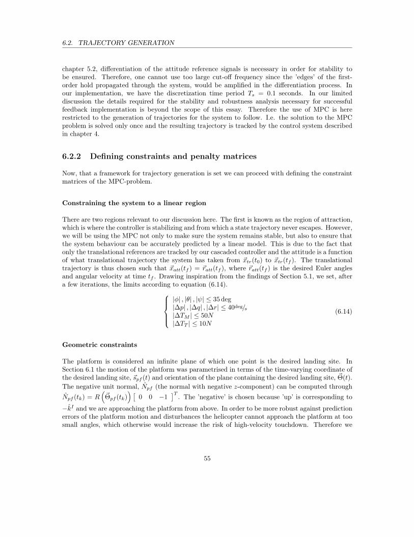
6.2. TRAJECTORY GENERATION
chapter 5.2, differentiation of the attitude reference signals is necessary in order for stability tobe ensured. Therefore, one cannot use too large cut-off frequency since the ’edges’ of the first-order hold propagated through the system, would be amplified in the differentiation process. Inour implementation, we have the discretization time period Ts = 0.1 seconds. In our limiteddiscussion the details required for the stability and robustness analysis necessary for successfulfeedback implementation is beyond the scope of this essay. Therefore the use of MPC is hererestricted to the generation of trajectories for the system to follow. I.e. the solution to the MPCproblem is solved only once and the resulting trajectory is tracked by the control system describedin chapter 4.
6.2.2 Defining constraints and penalty matrices
Now, that a framework for trajectory generation is set we can proceed with defining the constraintmatrices of the MPC-problem.
Constraining the system to a linear region
There are two regions relevant to our discussion here. The first is known as the region of attraction,which is where the controller is stabilizing and from which a state trajectory never escapes. However,we will be using the MPC not only to make sure the system remains stable, but also to ensure thatthe system behaviour can be accurately predicted by a linear model. This is due to the fact thatonly the translational references are tracked by our cascaded controller and the attitude is a functionof what translational trajectory the system has taken from ~xtr(t0) to ~xtr(tf ). The translationaltrajectory is thus chosen such that ~xatt(tf ) = ~ratt(tf ), where ~ratt(tf ) is the desired Euler anglesand angular velocity at time tf . Drawing inspiration from the findings of Section 5.1, we set, aftera few iterations, the limits according to equation (6.14).
|φ| , |θ| , |ψ| ≤ 35 deg|∆p| , |∆q| , |∆r| ≤ 40deg/s|∆TM | ≤ 50N|∆TT | ≤ 10N
(6.14)
Geometric constraints
The platform is considered an infinite plane of which one point is the desired landing site. InSection 6.1 the motion of the platform was parametrised in terms of the time-varying coordinate ofthe desired landing site, ~spf (t) and orientation of the plane containing the desired landing site, ~Θ(t).The negative unit normal, Npf (the normal with negative z-component) can be computed throughNpf (tk) = R
(~Θpf (tk)
) [0 0 −1
]T . The ’negative’ is chosen because ’up’ is corresponding to
−kI and we are approaching the platform from above. In order to be more robust against predictionerrors of the platform motion and disturbances the helicopter cannot approach the platform at toosmall angles, which otherwise would increase the risk of high-velocity touchdown. Therefore we
55
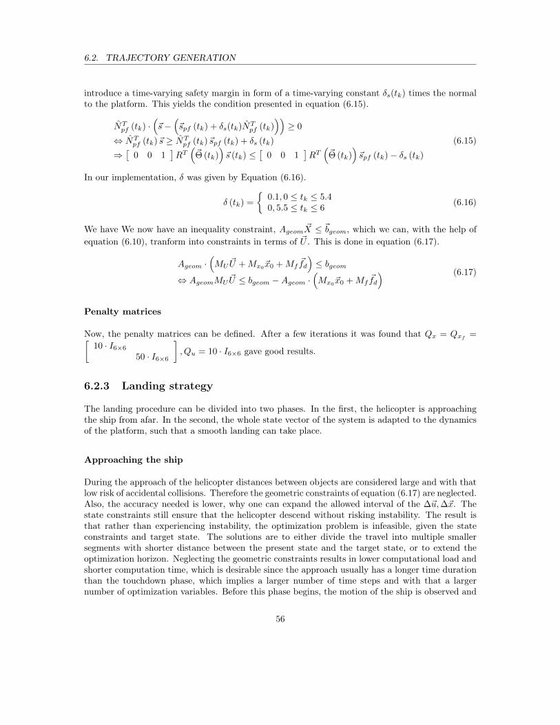
6.2. TRAJECTORY GENERATION
introduce a time-varying safety margin in form of a time-varying constant δs(tk) times the normalto the platform. This yields the condition presented in equation (6.15).
NTpf (tk) ·
(~s−
(~spf (tk) + δs(tk)NT
pf (tk)))≥ 0
⇔ NTpf (tk)~s ≥ NT
pf (tk)~spf (tk) + δs (tk)
⇒[
0 0 1]RT(~Θ (tk)
)~s (tk) ≤
[0 0 1
]RT(~Θ (tk)
)~spf (tk)− δs (tk)
(6.15)
In our implementation, δ was given by Equation (6.16).
δ (tk) =
{0.1, 0 ≤ tk ≤ 5.40, 5.5 ≤ tk ≤ 6
(6.16)
We have We now have an inequality constraint, Ageom ~X ≤ ~bgeom, which we can, with the help ofequation (6.10), tranform into constraints in terms of ~U . This is done in equation (6.17).
Ageom ·(MU
~U +Mx0~x0 +Mf
~fd
)≤ bgeom
⇔ AgeomMU~U ≤ bgeom −Ageom ·
(Mx0
~x0 +Mf~fd
) (6.17)
Penalty matrices
Now, the penalty matrices can be defined. After a few iterations it was found that Qx = Qxf =[10 · I6×6
50 · I6×6
], Qu = 10 · I6×6 gave good results.
6.2.3 Landing strategy
The landing procedure can be divided into two phases. In the first, the helicopter is approachingthe ship from afar. In the second, the whole state vector of the system is adapted to the dynamicsof the platform, such that a smooth landing can take place.
Approaching the ship
During the approach of the helicopter distances between objects are considered large and with thatlow risk of accidental collisions. Therefore the geometric constraints of equation (6.17) are neglected.Also, the accuracy needed is lower, why one can expand the allowed interval of the ∆~u,∆~x. Thestate constraints still ensure that the helicopter descend without risking instability. The result isthat rather than experiencing instability, the optimization problem is infeasible, given the stateconstraints and target state. The solutions are to either divide the travel into multiple smallersegments with shorter distance between the present state and the target state, or to extend theoptimization horizon. Neglecting the geometric constraints results in lower computational load andshorter computation time, which is desirable since the approach usually has a longer time durationthan the touchdown phase, which implies a larger number of time steps and with that a largernumber of optimization variables. Before this phase begins, the motion of the ship is observed and
56
6.3. DISCUSSION
an amplitude of the oscillatory part of the ship motion is estimated. The target state in this phasebelongs to the set of trimming points mentioned in section 4.4.1 (equation (4.43)) and chosen suchthat the helicopter would not touch the ship at any time throughout the ships periodic motion.When the approach is completed the actual touchdown procedure begins.
Touchdown
During this phase an MPC including the geometric constraints is used. The optimization horizonm ·Ts for the MPC determines the time instance the helicopter lands. The position and attitude ofthe ship is estimated up till that that time instance, which allows the generation of the geometricinequality constraints and the target equality constraint. Lastly the final MPC is computed.
6.3 Discussion
6.3.1 Feasibility of the MPC
One of the main issues with this approach is the lack of guarantee of feasibility of the posedoptimization problem. In fact, this problem was encountered under various conditions throughoutthe work. A solace is that this part of the MPC does not need to be computed in a rush. Thehelicopter is hoovering safely above the platform and repeated attempts on computing a feasibletrajectory can be made. Once this is done successfully, the touchdown phase can be initiated. Ifthe feasible set is empty for several attempts, this may be an indication of e.g. weather conditionsin which it is not advisable to attempt a landing, at least with the linear controller implemented inthis essay. However, as will be shown in section 7.1, the translational reference trajectory will betracked with relatively high accuracy. This means that for a platform only somewhat larger thanthe helicopter, we need not land in its center to ensure a successful landning. Instead of the targetequality equation (6.13), one could then expand the feasible region of the optimization problem byconstraining the target state to fulfill the equation of the platform plane, i.e.
Npf (tm) · (~s (tm)− ~spf (tm)) = 0,
together with additional inequality constraints
Apf~xm ≤ ~bpf . (6.18)
Equation (6.18) is chosen such that{~s (tm) : Apf~s (tm) ≤ ~bpf
}∩{~s (tm) : NT
pf · ~s (tm) = 0}
is a closed curve which defines the boundary of the allowed region of the platform in which thehelicopter can safely land. An expansion of the feasible region generally allows for a lower value ofthe objective function and/or increases the chance of feasibility of the optimization problem.
57
6.3. DISCUSSION
6.3.2 Disturbances
Even though the MPC-based trajectory is followed in a closed loop fashion the trajectory is staticand does not respond to prediction errors in the motion of the platform or in the motion of thehelicopter. In order to make the landing procedure more robust, one should therefore introduce afeedback involving the actual recorded motion of the platform and either the static trajectory orthe helicopters present state. If the helicopter is subjected to disturbances the trajectory mightstill take the helicopter to the desired position but with angular states different from the desired.Therefore the angular states must obviously be monitored continuously and checked against theplatform. Again, since the helicopter is underactuated, chances of recovery, without restarting thewhole touchdown procedure with an updated reference trajectory, are limited. Since there is atranslational safety margin, δs in the trajectory planning the helicopter should be relatively robustagainst bumping into the platform due to disturbances. However, a repelling potential could beincluded of the type in equation (6.19).
fpot
(~spf,c,~spf,c, ~s,~s
)= −kpot
Npf ·~srel|~srel|3
·(
2
πtan−1 (ksat [~s− ~sm])
)4
(6.19)
The vector ~srel denotes the vector from the helicopter to the closest point on the platform. Then,we augment the reference vector, ~sref (from section 4.3.2) to equation (6.20).
~s∗ref = ~sref + fpotNpf (6.20)
The appropriate modifications should then be carried out for the rest of the translational statereference vector (differentiaton and integration of equation (6.20)). The seemingly complicatedexpression in equation (6.19) can be explained in words as “unless you’re close to the target position,velocities directed against the platform together with small distances from the platform should resultin a reference position farther away from the platform”. However, the limited time did not allowus to implement such a potential, nor to investigate any properties of it. Again, if the potential(like the disturbance) affected the system for long enough time, the trajectory would again not leadto desired angular state at touchdown. Thus, the potential would rather be a means to avoid anunsuccessful landing rather then aiding a successful one. The effect of the potential would be samein the case of prediction errors of the platform.
6.3.3 Helicopter design and sensitivity to landing conditions
Another point worth noting is that since the main rotor is the main force generator, it is is notas much the Euler angles as the direction of kI that determines the acceleration of the helicopter.This means that the Euler angles may very well deviate considerably from the state trajectory ofEuler angles the MPC generates, even though kI is directed correctly as to produce the desiredaccelerations. For a successful landing to take place, it is only the vector kI that needs to be alignedwith the normal of the plane, as far as the attitude is concerned. In connection to the attitudecondition for a successful landing, stated in section 6.1, one can realize that the helicopter designis a trade-off between several different goals.
1. A decoupling of the dynamics in p, q from that in r would require zt = 0. This would in turnresult in a small distance between the tail-rotor and the platform at touchdown.
58
6.3. DISCUSSION
2. A mitigatation of the non-minimum phase property of the system would require minimizingthe tail-rotor thrust. For the required balancing of the reaction torque from the main rotor,this would in turn require an increase in |xt|. A large |xt| would then lead to a very smallallowed error in Θ, again not to damage the tail-rotor during touchdown.
59
Chapter 7
Results and Conclusions
7.1 Simulation results
In this chapter simulations of a landing is presented. To evaluate the degree of success of thelandings, a few error parameters are introduced, relating the state of the helicopter to the desiredtarget state at touchdown. The speeds normal and parallel to the platform is denoted by vnormand vpar, respectively. The distance from the desired to the actual touchdown position is denotedby se. Lastly, the angle between −kB and Npf at touchdown is denoted by αe.
The results from 14 different simulations are presented in table 7.1. In each simulation the initialposition is set to ~s =
[3 3 −8
]T and the touch-down phase is initiated at sz = −2. The worstcases for each error parameter is marked in bold. These are vnorm,max = 0.42 m/s, vpar,max = 0.40m/s, se,max = 5.0 cm and αe,max = 9.4◦.
To illustrate the entire landing procedure, simulations of approach and landing for the case ∆tpf = 0is depicted by figures 7.1, 7.3 and 7.2. Notice the discontinuity in the TPP-angles a and b infigure 7.1. It is likely due to a slight translational error between the final position of the approachtrajectory and the actual position of the helicopter, when the translational reference signal fromthe touchdown trajectory is set out. The helicopter is converging to the final reference positon ofthe approach trajectory when the first point of the new trajectory coincides with the present stateof the helicopter. In short, the helicopter must jam the brakes.
Figure 7.2 needs an explanation. It shows that the shortest distance between the platform and thehelicopter never subseeds 0 while having large velocities. Thus the helicopter never crashes intothe platform. The figure also shows that after approximately 6 seconds the landing occurs withtolerable impact velocities. Finally, figure 7.3 is a 3D visualization of the whole landing procedure.
60
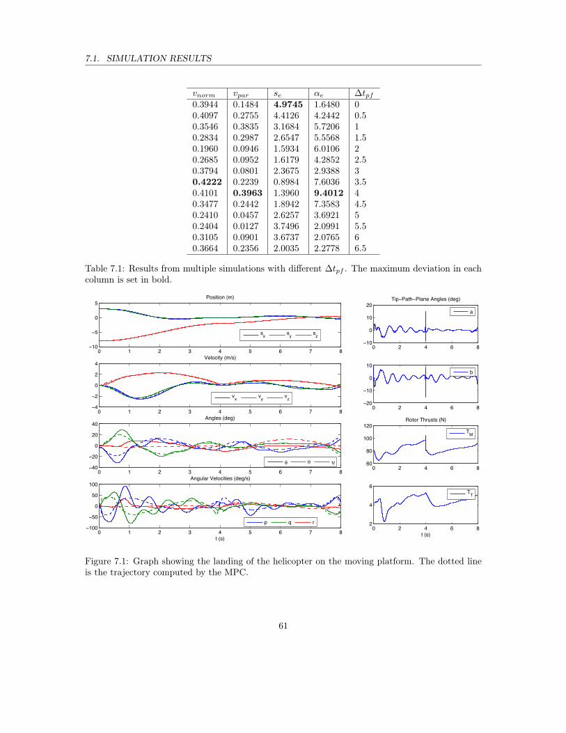
7.1. SIMULATION RESULTS
vnorm vpar se αe ∆tpf0.3944 0.1484 4.9745 1.6480 00.4097 0.2755 4.4126 4.2442 0.50.3546 0.3835 3.1684 5.7206 10.2834 0.2987 2.6547 5.5568 1.50.1960 0.0946 1.5934 6.0106 20.2685 0.0952 1.6179 4.2852 2.50.3794 0.0801 2.3675 2.9388 30.4222 0.2239 0.8984 7.6036 3.50.4101 0.3963 1.3960 9.4012 40.3477 0.2442 1.8942 7.3583 4.50.2410 0.0457 2.6257 3.6921 50.2404 0.0127 3.7496 2.0991 5.50.3105 0.0901 3.6737 2.0765 60.3664 0.2356 2.0035 2.2778 6.5
Table 7.1: Results from multiple simulations with different ∆tpf . The maximum deviation in eachcolumn is set in bold.
0 1 2 3 4 5 6 7 810
5
0
5Position (m)
sx sy sz
0 2 4 6 810
0
10
20Tip Path Plane Angles (deg)
a
0 1 2 3 4 5 6 7 84
2
0
2
4Velocity (m/s)
vx vy vz
0 2 4 6 820
10
0
10
b
0 1 2 3 4 5 6 7 840
20
0
20
40Angles (deg)
0 2 4 6 860
80
100
120Rotor Thrusts (N)
TM
0 1 2 3 4 5 6 7 8100
50
0
50
100
t (s)
Angular Velocities (deg/s)
p q r0 2 4 6 8
2
4
6
t (s)
TT
Figure 7.1: Graph showing the landing of the helicopter on the moving platform. The dotted lineis the trajectory computed by the MPC.
61
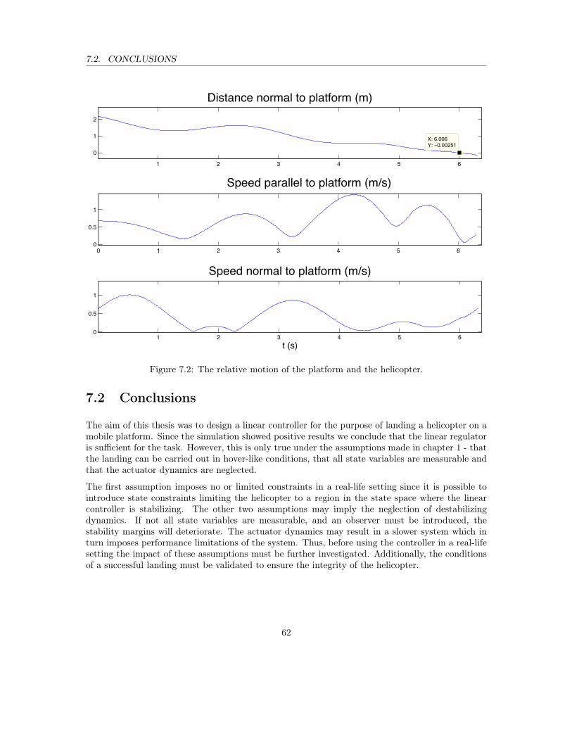
7.2. CONCLUSIONS
1 2 3 4 5 6
0
1
2
X: 6.006Y: 0.00251
Distance normal to platform (m)
0 1 2 3 4 5 60
0.5
1
Speed parallel to platform (m/s)
1 2 3 4 5 60
0.5
1
Speed normal to platform (m/s)
t (s)
Figure 7.2: The relative motion of the platform and the helicopter.
7.2 Conclusions
The aim of this thesis was to design a linear controller for the purpose of landing a helicopter on amobile platform. Since the simulation showed positive results we conclude that the linear regulatoris sufficient for the task. However, this is only true under the assumptions made in chapter 1 - thatthe landing can be carried out in hover-like conditions, that all state variables are measurable andthat the actuator dynamics are neglected.
The first assumption imposes no or limited constraints in a real-life setting since it is possible tointroduce state constraints limiting the helicopter to a region in the state space where the linearcontroller is stabilizing. The other two assumptions may imply the neglection of destabilizingdynamics. If not all state variables are measurable, and an observer must be introduced, thestability margins will deteriorate. The actuator dynamics may result in a slower system which inturn imposes performance limitations of the system. Thus, before using the controller in a real-lifesetting the impact of these assumptions must be further investigated. Additionally, the conditionsof a successful landing must be validated to ensure the integrity of the helicopter.
62
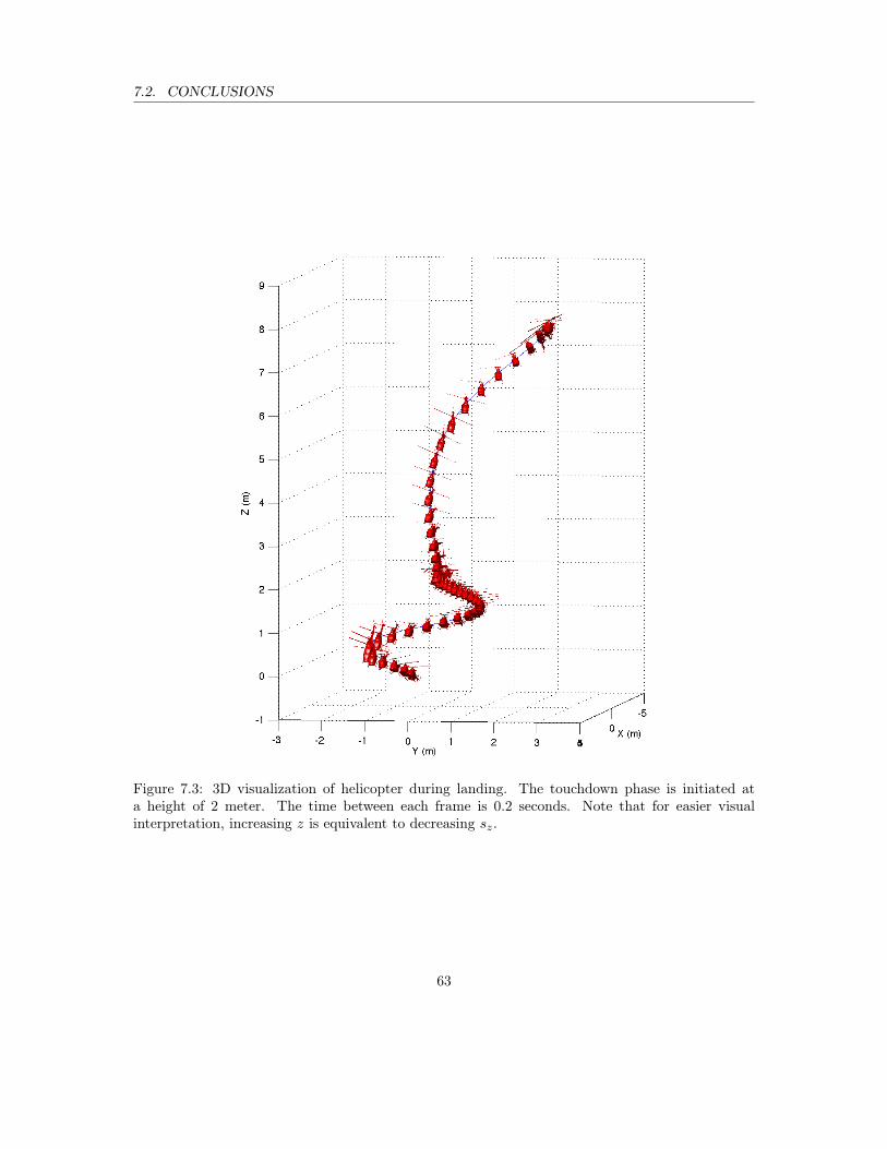
7.2. CONCLUSIONS
Figure 7.3: 3D visualization of helicopter during landing. The touchdown phase is initiated ata height of 2 meter. The time between each frame is 0.2 seconds. Note that for easier visualinterpretation, increasing z is equivalent to decreasing sz.
63

Bibliography
[1] N. Apazidis. Rigid body and analytical mechanics. Institutionen för mekanik, KTH, 2009.
[2] J. I. Askelin. UAV är dagens militära modeord. FOA-tidningen, 3, 1996.
[3] K. Byeongil, C. Yushin, K. Joongeup, H. Heegwon, and L. Manhyung. Design of 6-dof attitudecontroller of hovering model helicopter. In Industrial Electronics Society, 2004. IECON 2004.30th Annual Conference of IEEE, volume 1, pages 104 – 110, 2004.
[4] C.T. Chen. Linear System Theory and Design. Oxford University Press, 1999.
[5] T. Glad and L. Ljung. Reglerteori - flervariabla och olinjära metoder. Studentlitteratur, 1997.
[6] T. Glad and L. Ljung. Reglerteknik - grundläggande teori. Studentlitteratur, fourth edition,2006.
[7] J.C. Hunsaker and B.G Rightmire. Engineering applications of fluid mechanics. McGraw-Hill,1947.
[8] K.H. Khalil. Nonlinear systems. Prentice Hall, third edition, 2002.
[9] T. J. Koo and S. Sastry. Output tracking control design of a helicopter model based on approx-imate linearization. In Decision and Control, 1998. Proceedings of the 37th IEEE Conferenceon, volume 4, pages 3635–3640, 1998.
[10] J.B. Kuipers. Quaternions and rotation sequences. In Proceedings of the International Con-ference on Geometry, Integrability and Quantization, volume 1, pages 127–143. Coral Press,2000.
[11] S.R. Oh, K. Pathak, S.K. Agrawal, H.R. Pota, and M. Garratt. Approaches for a tether-guidedlanding of an autonomous helicopter. Robotics, IEEE Transactions on, 22(3):536 – 544, 2006.
[12] G.D. Padfield. Helicopter flight dynamics. Blackwell Science Ltd., 1996.
[13] I. A. Raptis and K. P. Valavanis. Linear and Nonlinear Control of Small-Scale UnmannedHelicopters. Springer, 2011.
[14] J. W. C. Robinson. Block backstepping for nonlinear flight control law design. In NonlinearAnalysis and Synthesis Techniques for Aircraft Control, volume 365 of Lecture Notes in Controland Information Sciences, pages 231–257. Springer, 2007.
64

BIBLIOGRAPHY
[15] J. Shin, K. Nonami, D. Fujiwara, and K. Hazawa. Model-based optimal attitude and positioningcontrol of small-scale unmanned helicopter. Robotica, 23(01):51–63, 2005.
[16] X. Yang, H. Pota, M. Garratt, and V. Ugrinovskii. Heave motion prediction for maritimeoperations of uavs. In Launch and Recovery (LARS) 2008 Proceedings, 2008.
65