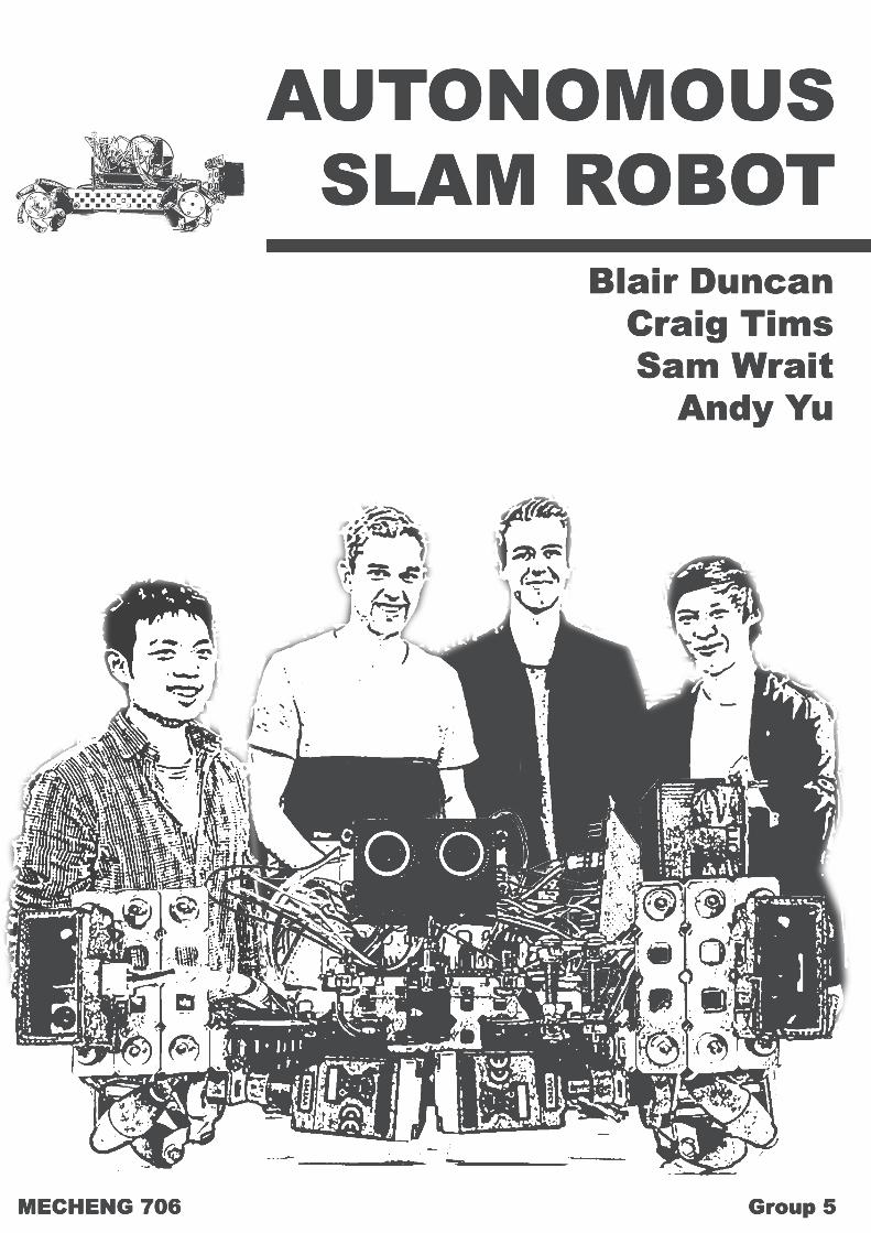
AUTONOMOUSSLAM ROBOT

Blair DuncanCraig TimsSam Wrait

Andy Yu

Group 5MECHENG 706

Executive Summary

Simultaneous Localisation and Mapping (SLAM) is a di�cult problem to solve. This isbecause of the cross dependency of both aspects of the problem: mapping and localisation.The aim of the project is to design autonomous robot system that incorporates the SLAMalgorithm to cover a room for the purpose of vacuum cleaning. This project involved manyaspects of the Mechatronics discipline; Mechanical design, hardware calibration and softwareintelligence. These aspects were simultaneously integrated throughout the whole project.

The hardware included four infrared(IR) ranging sensors, one ultrasonic ranging module,one motion processing unit (MPU), a servomotor, a bluetooth module and a partially builtrobot with 4 Mecanum wheels. These are used in combination to create sensory perceptionfor decision making processes and the resulting motion generated by the autonomous robot.

This report contains the methodologies and ideas behind finding a solution for the assignedproblem, including the thinking behind the path taken by the robot, obstacle detection andavoidance and mapping method.

Ultimately the demonstration run achieved perfect obstacle avoidance with a relatively quickrun. The coverage of the room was an issue however, as the robot lost its reference after amisalignment, resulting in only about 50% coverage. As such, there are aspects for improve-ment. The utilisation of the provided servomotor would help improve the robots ability todistinguish between obstacle and walls. More accurate and tolerant sensor signal processingcould help with reliability and reduce misalignment. Finally the application of full SLAM,where the created map if used to avoid with navigation and path optimisation would greatlyimprove the performance of the robot in a variety of courses.

ii

Contents

1 Introduction . . . . . . . . . . . . . . . . . . . . . . . . . . . . . . . . . . . . 12 Problem Description . . . . . . . . . . . . . . . . . . . . . . . . . . . . . . . 23 System Overview . . . . . . . . . . . . . . . . . . . . . . . . . . . . . . . . . 2

3.1 Robot Path . . . . . . . . . . . . . . . . . . . . . . . . . . . . . . . . 23.2 Sensor Placement . . . . . . . . . . . . . . . . . . . . . . . . . . . . . 23.3 Software & Hardware Integration . . . . . . . . . . . . . . . . . . . . 4

4 Hardware . . . . . . . . . . . . . . . . . . . . . . . . . . . . . . . . . . . . . 44.1 Short Range IR Sensors . . . . . . . . . . . . . . . . . . . . . . . . . 44.2 Long Range IR Sensors . . . . . . . . . . . . . . . . . . . . . . . . . . 54.3 Analogue Filter for IR Sensors . . . . . . . . . . . . . . . . . . . . . . 64.4 Sonar . . . . . . . . . . . . . . . . . . . . . . . . . . . . . . . . . . . 64.5 Motion Processing Unit . . . . . . . . . . . . . . . . . . . . . . . . . 74.6 Servomotor . . . . . . . . . . . . . . . . . . . . . . . . . . . . . . . . 8

5 Software . . . . . . . . . . . . . . . . . . . . . . . . . . . . . . . . . . . . . . 95.1 Sub-Functions . . . . . . . . . . . . . . . . . . . . . . . . . . . . . . . 95.2 Main States . . . . . . . . . . . . . . . . . . . . . . . . . . . . . . . . 115.3 Debugging Methods . . . . . . . . . . . . . . . . . . . . . . . . . . . 17

6 Localisation & Mapping . . . . . . . . . . . . . . . . . . . . . . . . . . . . . 186.1 LabVIEW . . . . . . . . . . . . . . . . . . . . . . . . . . . . . . . . . 186.2 Localisation . . . . . . . . . . . . . . . . . . . . . . . . . . . . . . . . 196.3 Mapping . . . . . . . . . . . . . . . . . . . . . . . . . . . . . . . . . . 22

7 Results . . . . . . . . . . . . . . . . . . . . . . . . . . . . . . . . . . . . . . . 258 Discussion . . . . . . . . . . . . . . . . . . . . . . . . . . . . . . . . . . . . . 26

8.1 Improvements . . . . . . . . . . . . . . . . . . . . . . . . . . . . . . . 269 Conclusion . . . . . . . . . . . . . . . . . . . . . . . . . . . . . . . . . . . . . 28References . . . . . . . . . . . . . . . . . . . . . . . . . . . . . . . . . . . . . . . . 29Appendices . . . . . . . . . . . . . . . . . . . . . . . . . . . . . . . . . . . . . . . 30

Software code . . . . . . . . . . . . . . . . . . . . . . . . . . . . . . . . . . . 30Drawings . . . . . . . . . . . . . . . . . . . . . . . . . . . . . . . . . . . . . . 41

iii

List of Figures

1 Conceptual Diagram of the SLAM Problem - involving information about the robot

state (s), odometry (u), sensor measurements (z), landmark positions (r) and environment

map (m) [1] . . . . . . . . . . . . . . . . . . . . . . . . . . . . . . . . . . . . . 12 Predetermined Inwards Spiral Path . . . . . . . . . . . . . . . . . . . . . . . 23 Sensor Placement . . . . . . . . . . . . . . . . . . . . . . . . . . . . . . . . . 34 Short Range IR Sensor Calibration . . . . . . . . . . . . . . . . . . . . . . . 45 Rectangular Casing for IR Sensors . . . . . . . . . . . . . . . . . . . . . . . . 56 Long Range IR Sensor Calibration . . . . . . . . . . . . . . . . . . . . . . . 57 A Low Pass Filter Implemented on Veroboard . . . . . . . . . . . . . . . . . 68 HC-SR04 Ultrasonic Sonar Sensor . . . . . . . . . . . . . . . . . . . . . . . . 69 Sonar Sensor Casing . . . . . . . . . . . . . . . . . . . . . . . . . . . . . . . 710 MPU-9150 Breakout Board . . . . . . . . . . . . . . . . . . . . . . . . . . . 711 MPU Case . . . . . . . . . . . . . . . . . . . . . . . . . . . . . . . . . . . . . 712 Servomotor Mount . . . . . . . . . . . . . . . . . . . . . . . . . . . . . . . . 813 IR Aligning (Red) vs. Yaw Aligning (Green) . . . . . . . . . . . . . . . . . . 1014 State Diagram . . . . . . . . . . . . . . . . . . . . . . . . . . . . . . . . . . . 1215 Wall Alignment . . . . . . . . . . . . . . . . . . . . . . . . . . . . . . . . . . 1316 Finding the Second Wall . . . . . . . . . . . . . . . . . . . . . . . . . . . . . 1317 Ideal Spiral Path with No Obstacles . . . . . . . . . . . . . . . . . . . . . . . 1418 Di↵erent Cases for Obstacle Detection . . . . . . . . . . . . . . . . . . . . . 1519 Robot Counting Four Large Changes in Long Range IR Sensor Readings . . 1620 Example Output being Read with TerminalBT . . . . . . . . . . . . . . . . . 1721 Reading Data from the Bluetooth Receiver in LabVIEW . . . . . . . . . . . 1822 Section of Code Sending Sensor Data to the LabVIEW Program . . . . . . . 1923 Layout of Sensor Readings in LabVIEW . . . . . . . . . . . . . . . . . . . . 1924 Formula Node Implementing the Kalman Filter . . . . . . . . . . . . . . . . 2225 Mapping cases . . . . . . . . . . . . . . . . . . . . . . . . . . . . . . . . . . . 2326 Corner Determination . . . . . . . . . . . . . . . . . . . . . . . . . . . . . . 2327 Combining Arrays to Produce the Map . . . . . . . . . . . . . . . . . . . . . 2428 An example map of a successful run . . . . . . . . . . . . . . . . . . . . . . . 2429 Demonstration Run Result . . . . . . . . . . . . . . . . . . . . . . . . . . . . 2530 State Diagram . . . . . . . . . . . . . . . . . . . . . . . . . . . . . . . . . . . 2731 Code to Run the Ultrasonic Sonar Sensor . . . . . . . . . . . . . . . . . . . . 3032 The ’Rotate’ Function. Used to Rotate 90� . . . . . . . . . . . . . . . . . . . 3033 The ’forward straight’ Function Uses the MPU . . . . . . . . . . . . . . . . . 3134 The ’strafe straight’ Function . . . . . . . . . . . . . . . . . . . . . . . . . . 32

iv

35 The ’check straight’ Function. Uses the Long Range IR Sensors . . . . . . . 3236 The ’avoid left’ Function . . . . . . . . . . . . . . . . . . . . . . . . . . . . . 3337 The ’align wall’ Function . . . . . . . . . . . . . . . . . . . . . . . . . . . . . 3438 The ’find yaw’ Function . . . . . . . . . . . . . . . . . . . . . . . . . . . . . 3439 The First Half of ’find corner’ Function . . . . . . . . . . . . . . . . . . . . . 3540 The Second Half of ’find corner’ Function . . . . . . . . . . . . . . . . . . . . 3641 The First Part of the ’spiraling’ Function . . . . . . . . . . . . . . . . . . . . 3742 The Second Part of the ’spiraling’ Function . . . . . . . . . . . . . . . . . . . 3843 The Third Part of the ’spiraling’ Function . . . . . . . . . . . . . . . . . . . 3944 The Fourth Part of the ’spiraling’ Function . . . . . . . . . . . . . . . . . . . 4045 LabView Code - I/O and String Splitting . . . . . . . . . . . . . . . . . . . . 4146 LabView Code - Kalman Filter and Map Plotting . . . . . . . . . . . . . . . 41

v

1 Introduction

Simultaneous Localisation and Mapping (SLAM) involves finding the location of a movingobject in an unknown environment while at the same time creating a map of it. The aimof this project is to create an autonomous robot capable of performing SLAM to ‘vacuumclean’ a small, controlled environment. An Arduino controlled, omnidirectional robot and asmall range of sensors are provided to achieve this aim. In order to function as a vacuumcleaner, the robot has three main goals. It must cover as much of the room as possible, whileavoiding any obstacles. This coverage should be completed in as short a time as possible.

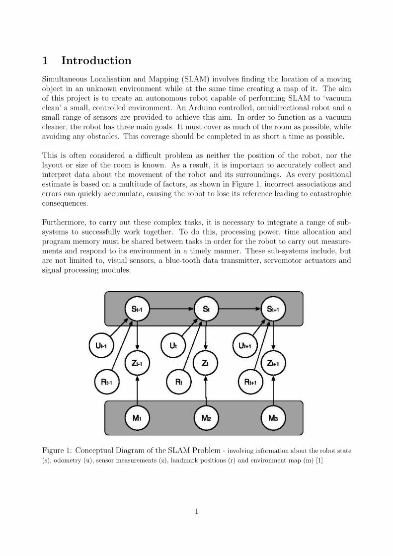
This is often considered a di�cult problem as neither the position of the robot, nor thelayout or size of the room is known. As a result, it is important to accurately collect andinterpret data about the movement of the robot and its surroundings. As every positionalestimate is based on a multitude of factors, as shown in Figure 1, incorrect associations anderrors can quickly accumulate, causing the robot to lose its reference leading to catastrophicconsequences.

Furthermore, to carry out these complex tasks, it is necessary to integrate a range of sub-systems to successfully work together. To do this, processing power, time allocation andprogram memory must be shared between tasks in order for the robot to carry out measure-ments and respond to its environment in a timely manner. These sub-systems include, butare not limited to, visual sensors, a blue-tooth data transmitter, servomotor actuators andsignal processing modules.

Figure 1: Conceptual Diagram of the SLAM Problem - involving information about the robot state

(s), odometry (u), sensor measurements (z), landmark positions (r) and environment map (m) [1]

1

2 Problem Description

The main requirement of this project is to design and build an autonomous robot capableof Simultaneous Localisation and Mapping (SLAM) to vacuum clean a rectangular room.The robot must avoid making contact with any obstacles or walls it comes across. A par-tially completed mechanical design comprising of a chassis, four motors drivers attached toMecanum wheels, a power supply and an Arduino Mega. To complete this project a seriesof sensors were mounted and software was written to carry out the required task. Limita-tions on hardware included no more than four infrared (IR) sensors, one ultrasonic sonar, aservomotor, a Motion Processing Unit (MPU) and a blue-tooth module for communicationwith a computer or phone.

3 System Overview

3.1 Robot Path

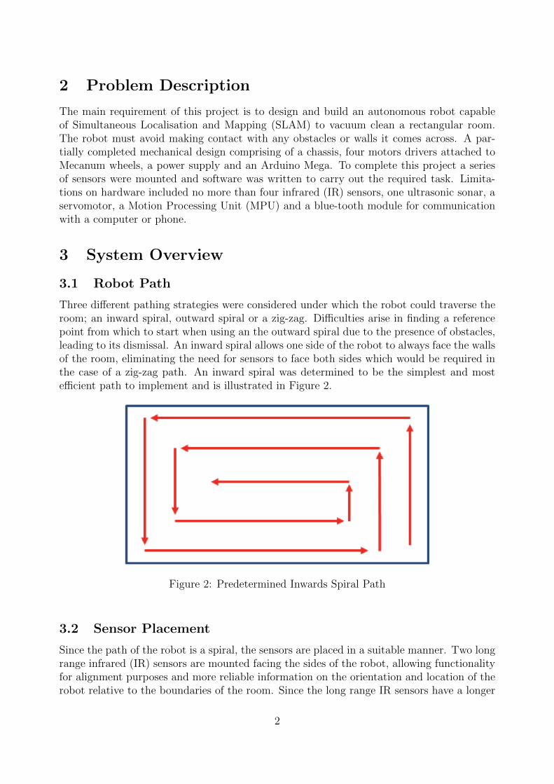
Three di↵erent pathing strategies were considered under which the robot could traverse theroom; an inward spiral, outward spiral or a zig-zag. Di�culties arise in finding a referencepoint from which to start when using an the outward spiral due to the presence of obstacles,leading to its dismissal. An inward spiral allows one side of the robot to always face the wallsof the room, eliminating the need for sensors to face both sides which would be required inthe case of a zig-zag path. An inward spiral was determined to be the simplest and moste�cient path to implement and is illustrated in Figure 2.

Figure 2: Predetermined Inwards Spiral Path

3.2 Sensor Placement

Since the path of the robot is a spiral, the sensors are placed in a suitable manner. Two longrange infrared (IR) sensors are mounted facing the sides of the robot, allowing functionalityfor alignment purposes and more reliable information on the orientation and location of therobot relative to the boundaries of the room. Since the long range IR sensors have a longer

2

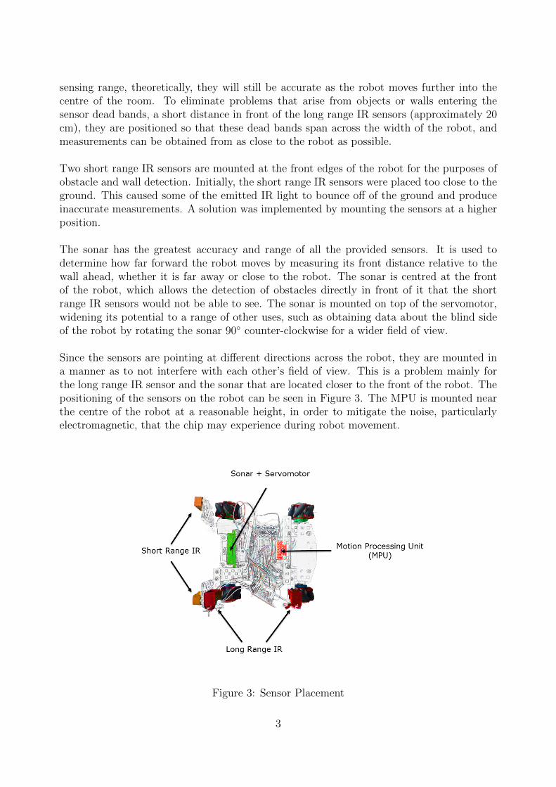
sensing range, theoretically, they will still be accurate as the robot moves further into thecentre of the room. To eliminate problems that arise from objects or walls entering thesensor dead bands, a short distance in front of the long range IR sensors (approximately 20cm), they are positioned so that these dead bands span across the width of the robot, andmeasurements can be obtained from as close to the robot as possible.

Two short range IR sensors are mounted at the front edges of the robot for the purposes ofobstacle and wall detection. Initially, the short range IR sensors were placed too close to theground. This caused some of the emitted IR light to bounce o↵ of the ground and produceinaccurate measurements. A solution was implemented by mounting the sensors at a higherposition.

The sonar has the greatest accuracy and range of all the provided sensors. It is used todetermine how far forward the robot moves by measuring its front distance relative to thewall ahead, whether it is far away or close to the robot. The sonar is centred at the frontof the robot, which allows the detection of obstacles directly in front of it that the shortrange IR sensors would not be able to see. The sonar is mounted on top of the servomotor,widening its potential to a range of other uses, such as obtaining data about the blind sideof the robot by rotating the sonar 90� counter-clockwise for a wider field of view.

Since the sensors are pointing at di↵erent directions across the robot, they are mounted ina manner as to not interfere with each other’s field of view. This is a problem mainly forthe long range IR sensor and the sonar that are located closer to the front of the robot. Thepositioning of the sensors on the robot can be seen in Figure 3. The MPU is mounted nearthe centre of the robot at a reasonable height, in order to mitigate the noise, particularlyelectromagnetic, that the chip may experience during robot movement.

Figure 3: Sensor Placement

3

3.3 Software & Hardware Integration

The software for the processing of the sensor signals and the actuation of the robot shouldaccommodate for how the sensors are mounted. This is done by adding o↵sets, obtainingbest fit equations and limiting the allowable ranges of the sensed signals using saturationlevels.

4 Hardware

4.1 Short Range IR Sensors

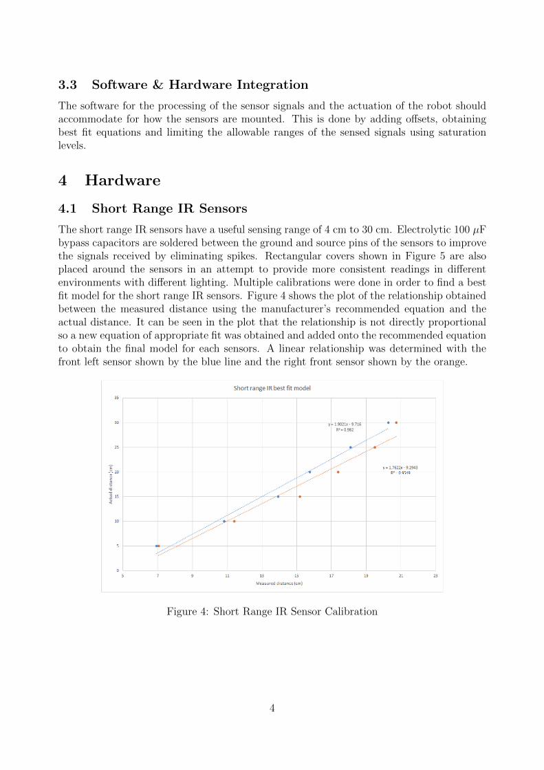
The short range IR sensors have a useful sensing range of 4 cm to 30 cm. Electrolytic 100 µFbypass capacitors are soldered between the ground and source pins of the sensors to improvethe signals received by eliminating spikes. Rectangular covers shown in Figure 5 are alsoplaced around the sensors in an attempt to provide more consistent readings in di↵erentenvironments with di↵erent lighting. Multiple calibrations were done in order to find a bestfit model for the short range IR sensors. Figure 4 shows the plot of the relationship obtainedbetween the measured distance using the manufacturer’s recommended equation and theactual distance. It can be seen in the plot that the relationship is not directly proportionalso a new equation of appropriate fit was obtained and added onto the recommended equationto obtain the final model for each sensors. A linear relationship was determined with thefront left sensor shown by the blue line and the right front sensor shown by the orange.

Figure 4: Short Range IR Sensor Calibration

4

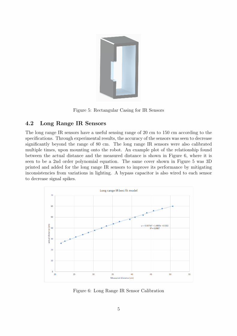
Figure 5: Rectangular Casing for IR Sensors

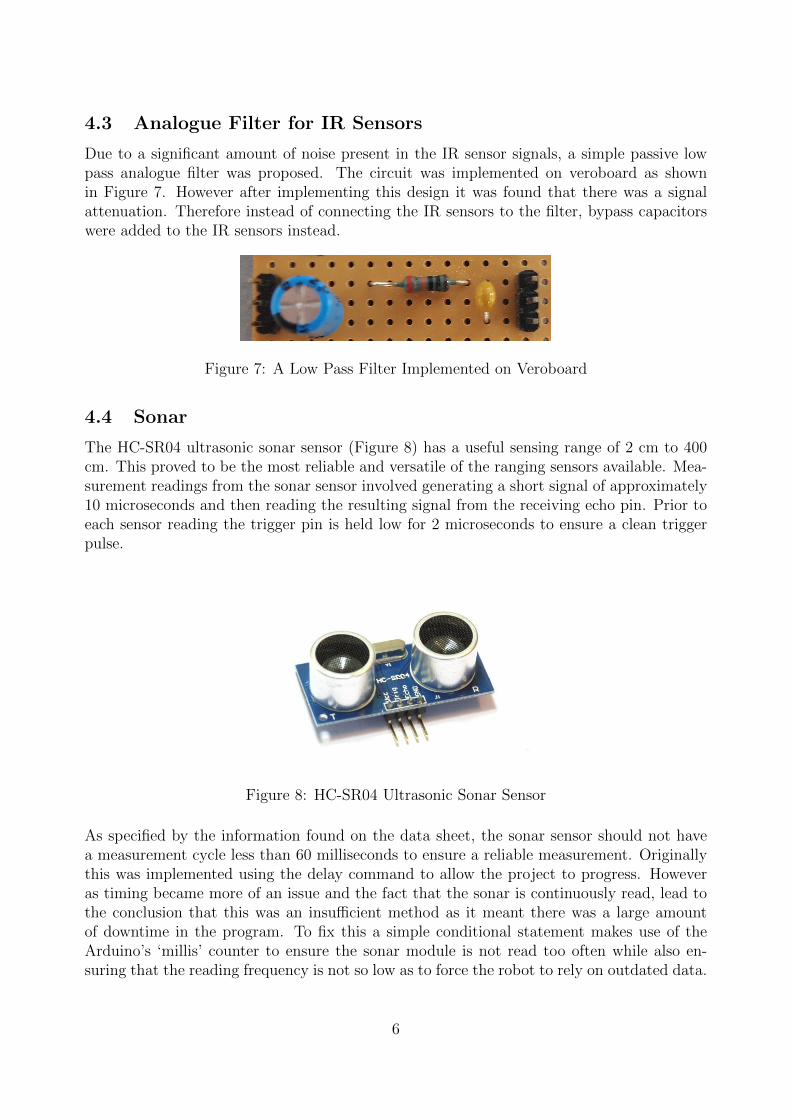
4.2 Long Range IR Sensors

The long range IR sensors have a useful sensing range of 20 cm to 150 cm according to thespecifications. Through experimental results, the accuracy of the sensors was seen to decreasesignificantly beyond the range of 80 cm. The long range IR sensors were also calibratedmultiple times, upon mounting onto the robot. An example plot of the relationship foundbetween the actual distance and the measured distance is shown in Figure 6, where it isseen to be a 2nd order polynomial equation. The same cover shown in Figure 5 was 3Dprinted and added for the long range IR sensors to improve its performance by mitigatinginconsistencies from variations in lighting. A bypass capacitor is also wired to each sensorto decrease signal spikes.

Figure 6: Long Range IR Sensor Calibration

5

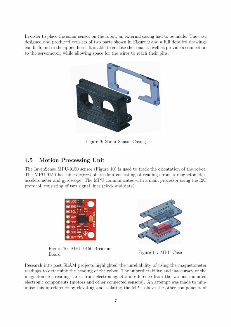
4.3 Analogue Filter for IR Sensors

Due to a significant amount of noise present in the IR sensor signals, a simple passive lowpass analogue filter was proposed. The circuit was implemented on veroboard as shownin Figure 7. However after implementing this design it was found that there was a signalattenuation. Therefore instead of connecting the IR sensors to the filter, bypass capacitorswere added to the IR sensors instead.

Figure 7: A Low Pass Filter Implemented on Veroboard

4.4 Sonar

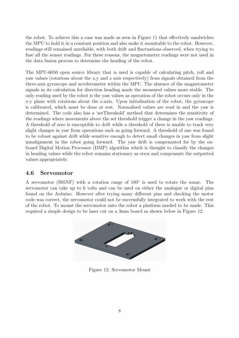
The HC-SR04 ultrasonic sonar sensor (Figure 8) has a useful sensing range of 2 cm to 400cm. This proved to be the most reliable and versatile of the ranging sensors available. Mea-surement readings from the sonar sensor involved generating a short signal of approximately10 microseconds and then reading the resulting signal from the receiving echo pin. Prior toeach sensor reading the trigger pin is held low for 2 microseconds to ensure a clean triggerpulse.

Figure 8: HC-SR04 Ultrasonic Sonar Sensor

As specified by the information found on the data sheet, the sonar sensor should not havea measurement cycle less than 60 milliseconds to ensure a reliable measurement. Originallythis was implemented using the delay command to allow the project to progress. Howeveras timing became more of an issue and the fact that the sonar is continuously read, lead tothe conclusion that this was an insu�cient method as it meant there was a large amountof downtime in the program. To fix this a simple conditional statement makes use of theArduino’s ‘millis’ counter to ensure the sonar module is not read too often while also en-suring that the reading frequency is not so low as to force the robot to rely on outdated data.

6

In order to place the sonar sensor on the robot, an external casing had to be made. The casedesigned and produced consists of two parts shown in Figure 9 and a full detailed drawingscan be found in the appendices. It is able to enclose the sonar as well as provide a connectionto the servomotor, while allowing space for the wires to reach their pins.

Figure 9: Sonar Sensor Casing

4.5 Motion Processing Unit

The InvenSense MPU-9150 sensor (Figure 10) is used to track the orientation of the robot.The MPU-9150 has nine-degrees of freedom consisting of readings from a magnetometer,accelerometer and gyroscope. The MPU communicates with a main processor using the I2Cprotocol, consisting of two signal lines (clock and data).

Figure 10: MPU-9150 BreakoutBoard Figure 11: MPU Case

Research into past SLAM projects highlighted the unreliability of using the magnetometerreadings to determine the heading of the robot. The unpredictability and inaccuracy of themagnetometer readings arise from electromagnetic interference from the various mountedelectronic components (motors and other connected sensors). An attempt was made to min-imise this interference by elevating and isolating the MPU above the other components of

7

the robot. To achieve this a case was made as seen in Figure 11 that e↵ectively sandwichesthe MPU to hold it in a constant position and also make it mountable to the robot. However,readings still remained unreliable, with both drift and fluctuations observed, when trying tofuse all the sensor readings. For these reasons, the magnetometer readings were not used inthe data fusion process to determine the heading of the robot.

The MPU-6050 open source library that is used is capable of calculating pitch, roll andyaw values (rotations about the x,y and z axis respectively) from signals obtained from thethree-axis gyroscope and accelerometer within the MPU. The absence of the magnetometersignals in its calculation for direction heading made the measured values more stable. Theonly reading used by the robot is the yaw values as operation of the robot occurs only in thex-y plane with rotations about the z-axis. Upon initialisation of the robot, the gyroscopeis calibrated, which must be done at rest. Normalised values are read in and the yaw isdetermined. The code also has a ‘setThreshold’ method that determines the sensitivity ofthe readings where movements above the set threshold trigger a change in the yaw readings.A threshold of zero is susceptible to drift while a threshold of three is unable to track veryslight changes in yaw from operations such as going forward. A threshold of one was foundto be robust against drift while sensitive enough to detect small changes in yaw from slightmisalignment in the robot going forward. The yaw drift is compensated for by the on-board Digital Motion Processor (DMP) algorithm which is thought to classify the changesin heading values while the robot remains stationary as error and compensate the outputtedvalues appropriately.

4.6 Servomotor

A servomotor (S05NF) with a rotation range of 180� is used to rotate the sonar. Theservomotor can take up to 6 volts and can be used on either the analogue or digital pinsfound on the Arduino. However after trying many di↵erent pins and checking the motorcode was correct, the servomotor could not be successfully integrated to work with the restof the robot. To mount the servomotor onto the robot a platform needed to be made. Thisrequired a simple design to be laser cut on a 3mm board as shown below in Figure 12.

Figure 12: Servomotor Mount

8

5 Software

5.1 Sub-Functions

Sub-functions were written for robot to produce simple motions that would allow it to nav-igate its way through the room. This includes going forward, rotating, strafing and aligningagainst the wall. These functions utilise simple closed loop control with proportional gainsto prevent drift due to unequal friction in the wheels and inconsistencies of the servomotors.All code mentioned in this section can be found in the appendices.

Forward Straight

The robot had di�culty maintaining a straight line when moving forward due to the variablefriction between the Mecanum wheels and the room floor as well within the motors them-selves. A forward straight function then had to be determined that would allow the robotto maintain a straight path. The function utilises a proportional controller to maintain theyaw value of the robot within a certain range.

Yaw AligningUtilisation of the MPU’s yaw values meant that continuous tracking of the robot direc-tion could be achieved and any deviations from the set direction could be adjusted for bya controller that would determine an appropriate response. A proportional controller wasdeveloped that measured the error as the di↵erence between the measured yaw value andreference yaw value given. The reference yaw value is placed in a dead band to preventunstable oscillations from continuous minor changes around the reference value. The deadband is defined as the reference yaw value +/- 2� and the error is measured from the edgesof this band. The controller response involves a rotation of the robot proportional to theerror in order to correct the heading of the robot. Use of the yaw for a straight line howeveris not always reliable when incorporated with the other functions as the reference yaw givenis not always at a parallel heading to the wall.

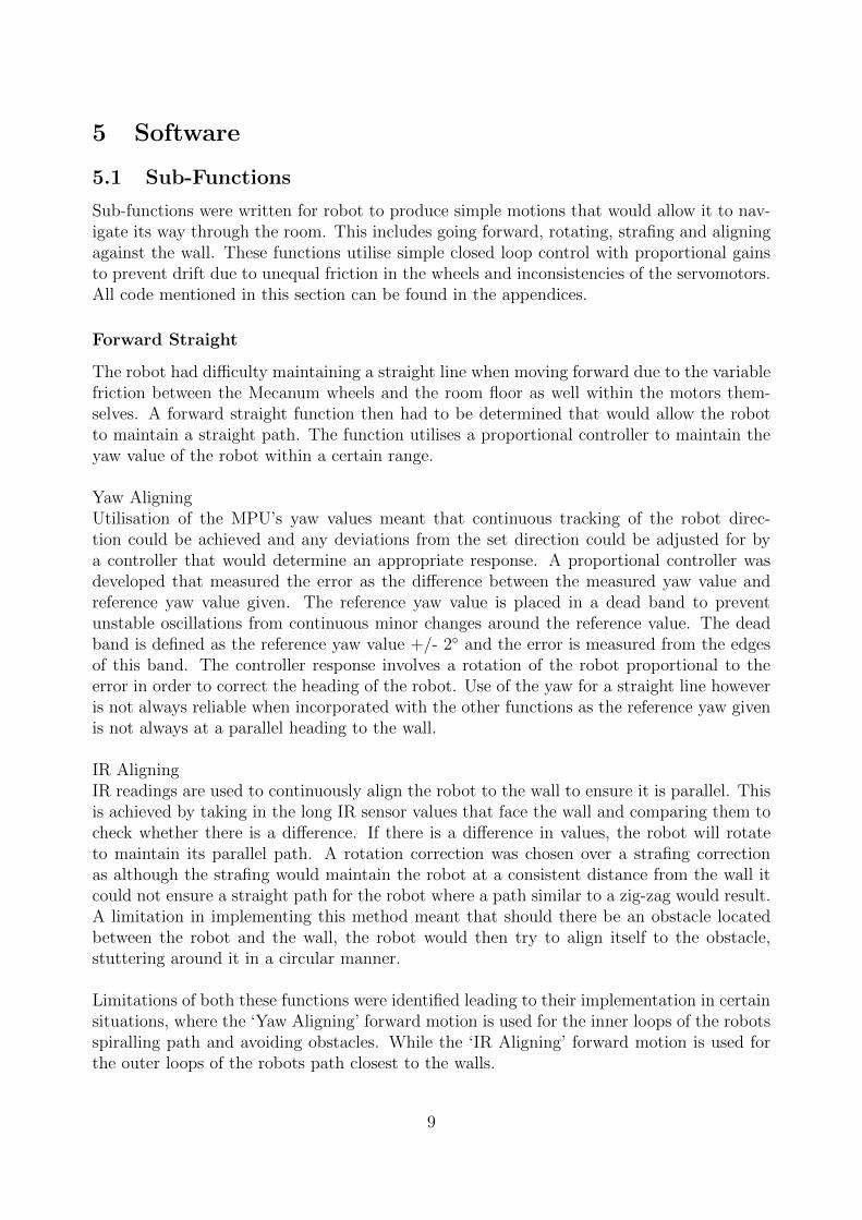
IR AligningIR readings are used to continuously align the robot to the wall to ensure it is parallel. Thisis achieved by taking in the long IR sensor values that face the wall and comparing them tocheck whether there is a di↵erence. If there is a di↵erence in values, the robot will rotateto maintain its parallel path. A rotation correction was chosen over a strafing correctionas although the strafing would maintain the robot at a consistent distance from the wall itcould not ensure a straight path for the robot where a path similar to a zig-zag would result.A limitation in implementing this method meant that should there be an obstacle locatedbetween the robot and the wall, the robot would then try to align itself to the obstacle,stuttering around it in a circular manner.

Limitations of both these functions were identified leading to their implementation in certainsituations, where the ‘Yaw Aligning’ forward motion is used for the inner loops of the robotsspiralling path and avoiding obstacles. While the ‘IR Aligning’ forward motion is used forthe outer loops of the robots path closest to the walls.

9

Figure 13: IR Aligning (Red) vs. Yaw Aligning (Green)

Strafe Straight

Similar to the problems faced in maintaining a straight line moving forward, the robot alsostruggled to strafe in a consistent direction. The inaccuracy of the strafe movement impactedon the performance of the forward straight function mentioned earlier as the reference yawpassed to it was inaccurate. A function is implemented that takes in a reference yaw anda strafe direction to maintain a constant heading of the car parallel to the wall. Althoughthe strafe can still result in a diagonal since the robot is still facing forward the impact onthe proceeding forward straights with yaw will be less impacted and achieve a better path.Yaw is used instead of IR readings to keep the robot parallel to the wall during a strafedue to it being a simpler calculation where only deviations from the reference yaw need tobe accounted for as opposed to measuring a consistent rate of change between the two IRsensors.

Rotate

The rotate function utilises a proportional control and sensor feedback from the MPU toproduce a controlled turn of the robot. This is done by continuously calculating the di↵er-ence between the robot’s current yaw value and the yaw value it is meant to be moving too.This di↵erence is then multiplied by a proportional gain. As this function is solely used torotate through 90� turns on corners, it was tuned for this use. It was found that a smallgain of 6.5 was ideal for a 90� turn. Since the rotate function can not handle overshoot,a secondary check was added after each time the rotate function was called to ensure thatrotate function hadn’t over or under turned. As the MPU isn’t perfectly accurate, the robotneeds to align to the wall after calling the rotate function.

This method above is our final and most successful rotation method however it is not the firstmethod attempted. The first method involved rotating the robot for a set amount of time(1.5 seconds) before aligning it to the wall. This method proved to be relatively successful,however other methods were explored that tried to improve upon this.

10

The second method that was attempted was unsuccessful. This method used the for-ward straight function to turn 90� and then in the same function move forward. Howeverdue to inaccuracies with the MPU, there was far too much error even when the robot aligneditself before turning. This method could have potentially worked if the program incorporateda strafe function to move either closer or further away from the wall when needed.

Wall Alignment

Unreliability of the rotate function due to the insensitivity of the MPU meant that after therotate function has been run the robot is not always reliably aligned with the wall. Thismisalignment causes problems for the forward straight yaw aligning function where it willmaintain the misalignment during the whole length of its straight path and never correct toalign with the wall. The wall alignment function is implemented to remove this problem,aligning the robot against the wall after a rotation using both wall facing long range IRsensors.

The readings from these sensors are passed into the alignment function, and the di↵erencebetween them designated as the error. Proportional control is then implemented to turn therobot clockwise or counterclockwise, until the sensor readings are within 0.5 cm. The gain ofthe proportional control was tuned to minimise overshoot, and an upper limit is also placedon the control value sent to the servos. Once this 0.5 cm condition is reached, the functionoutputs a true boolean indicating it has aligned.

Testing indicated that as the readings had a tendency to fluctuate, upon occasion the sensorvalues would briefly come between 0.5 cm , even when the robot didn’t align. As a result, a100 ms delay was implemented to check, after which the readings were checked for alignmentagain. If they were no longer within 0.5 cm, the alignment code was run again. The wholeprocess has a timeout of 1 second to stop the robot oscillating endlessly in an e↵ort to align.This function can be seen as ’align wall’ in the appendices.

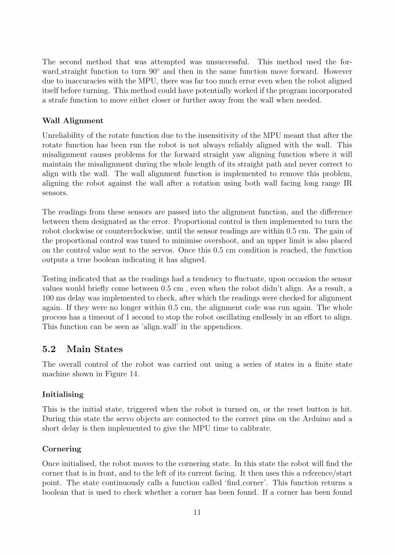
5.2 Main States

The overall control of the robot was carried out using a series of states in a finite statemachine shown in Figure 14.

Initialising

This is the initial state, triggered when the robot is turned on, or the reset button is hit.During this state the servo objects are connected to the correct pins on the Arduino and ashort delay is then implemented to give the MPU time to calibrate.

Cornering

Once initialised, the robot moves to the cornering state. In this state the robot will find thecorner that is in front, and to the left of its current facing. It then uses this a reference/startpoint. The state continuously calls a function called ‘find corner’. This function returns aboolean that is used to check whether a corner has been found. If a corner has been found

11

Figure 14: State Diagram

the program exits the ‘cornering’ state and enters ‘spiraling’.

Find corner works by first looking for a wall. To do this it will move forward while contin-uously monitoring the two from IR (short range) sensors. Once one of the front IR sensorsreads a value below a threshold value (10 cm) the robot will align itself to the wall using thefrom IR sensors.

To align itself to the wall, the robot continues to read the front IR sensors. It compares thesevalues using the align wall function mentioned in section 5.1. However after testing this codemultiple times it was found the robot could not su�ciently align to the wall leading to asecondary alignment check being implemented This check compares the two front IR sensorsand ensures the di↵erence between them is no more than 0.5 cm. If the di↵erence is notbelow 0.5 cm the program will call align wall again. Due to the reasonably low proportionalgain used in align wall, the robot struggles to make adjustments when the di↵erence betweenthe two IR’s are low. This means the robot would sometimes get stuck trying to align toa wall because it couldn’t supply a large enough voltage to the motors to overcome theirstarting torque. To counter this, Arduino’s ’millis()’ counter was used to ensure the robotdid not spent more than 0.75 seconds to align to the wall. If the robot took too long or wassu�ciently aligned, it would break out of this alignment loop.

To find a corner, the robot needs to find a second wall. To achieve this it first rotates 90� by

12

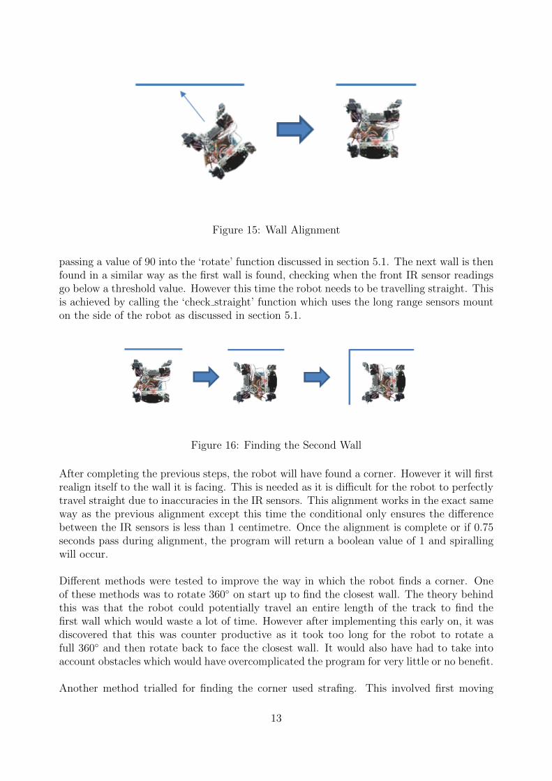
Figure 15: Wall Alignment

passing a value of 90 into the ‘rotate’ function discussed in section 5.1. The next wall is thenfound in a similar way as the first wall is found, checking when the front IR sensor readingsgo below a threshold value. However this time the robot needs to be travelling straight. Thisis achieved by calling the ‘check straight’ function which uses the long range sensors mounton the side of the robot as discussed in section 5.1.

Figure 16: Finding the Second Wall

After completing the previous steps, the robot will have found a corner. However it will firstrealign itself to the wall it is facing. This is needed as it is di�cult for the robot to perfectlytravel straight due to inaccuracies in the IR sensors. This alignment works in the exact sameway as the previous alignment except this time the conditional only ensures the di↵erencebetween the IR sensors is less than 1 centimetre. Once the alignment is complete or if 0.75seconds pass during alignment, the program will return a boolean value of 1 and spirallingwill occur.

Di↵erent methods were tested to improve the way in which the robot finds a corner. Oneof these methods was to rotate 360� on start up to find the closest wall. The theory behindthis was that the robot could potentially travel an entire length of the track to find thefirst wall which would waste a lot of time. However after implementing this early on, it wasdiscovered that this was counter productive as it took too long for the robot to rotate afull 360� and then rotate back to face the closest wall. It would also have had to take intoaccount obstacles which would have overcomplicated the program for very little or no benefit.

Another method trialled for finding the corner used strafing. This involved first moving

13

forward until a wall is found, aligning to this wall and then strafing to the right until thesecond wall is found. The theory behind this was the robot would require one less turn andalignment, saving a small amount of time. However strafing is slower than moving forwardwhich counteracted the time saved. It also had the problem of colliding with obstacles placedon walls as it had no way of detecting obstacles with the two side IR sensors.

Spiralling

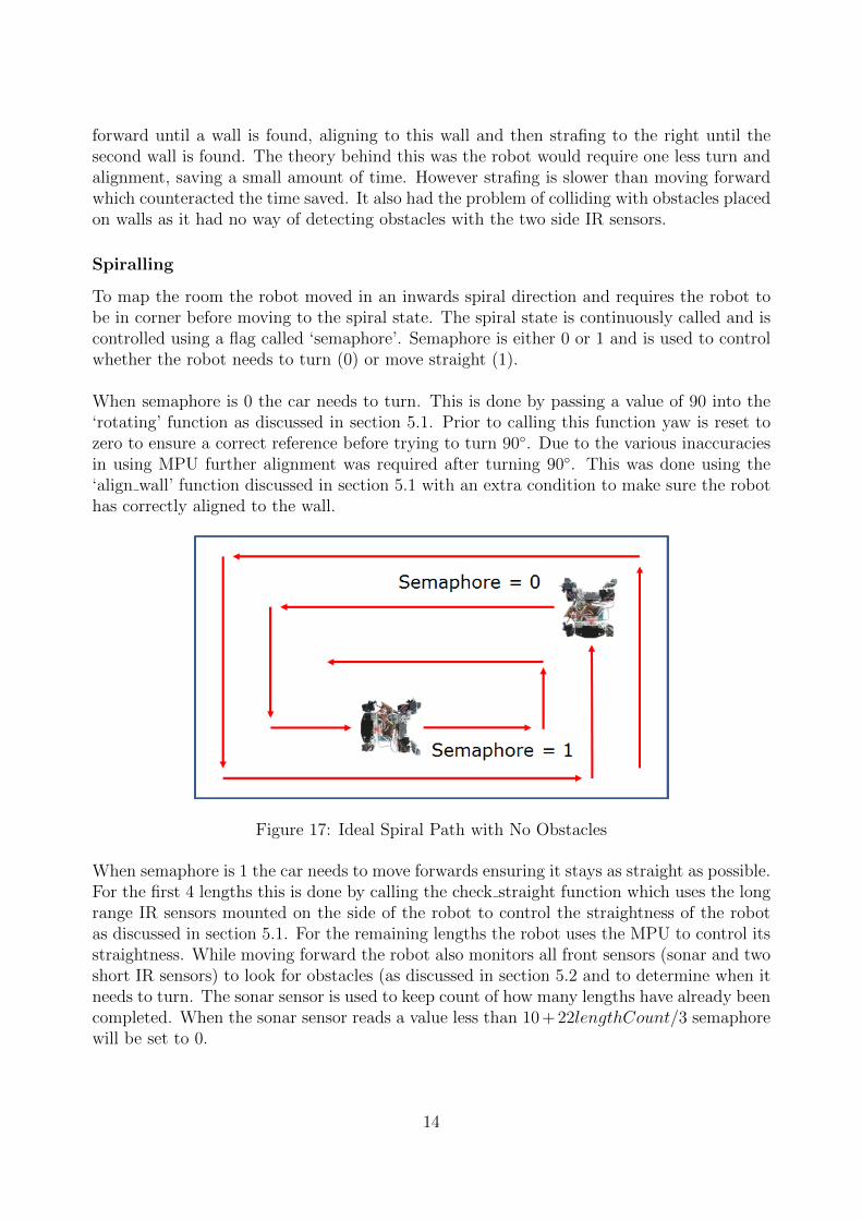
To map the room the robot moved in an inwards spiral direction and requires the robot tobe in corner before moving to the spiral state. The spiral state is continuously called and iscontrolled using a flag called ‘semaphore’. Semaphore is either 0 or 1 and is used to controlwhether the robot needs to turn (0) or move straight (1).

When semaphore is 0 the car needs to turn. This is done by passing a value of 90 into the‘rotating’ function as discussed in section 5.1. Prior to calling this function yaw is reset tozero to ensure a correct reference before trying to turn 90�. Due to the various inaccuraciesin using MPU further alignment was required after turning 90�. This was done using the‘align wall’ function discussed in section 5.1 with an extra condition to make sure the robothas correctly aligned to the wall.

Figure 17: Ideal Spiral Path with No Obstacles

When semaphore is 1 the car needs to move forwards ensuring it stays as straight as possible.For the first 4 lengths this is done by calling the check straight function which uses the longrange IR sensors mounted on the side of the robot to control the straightness of the robotas discussed in section 5.1. For the remaining lengths the robot uses the MPU to control itsstraightness. While moving forward the robot also monitors all front sensors (sonar and twoshort IR sensors) to look for obstacles (as discussed in section 5.2 and to determine when itneeds to turn. The sonar sensor is used to keep count of how many lengths have already beencompleted. When the sonar sensor reads a value less than 10+22lengthCount/3 semaphorewill be set to 0.

14

Obstacle Detection

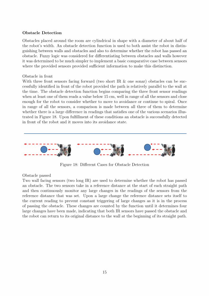
Obstacles placed around the room are cylindrical in shape with a diameter of about half ofthe robot’s width. An obstacle detection function is used to both assist the robot in distin-guishing between walls and obstacles and also to determine whether the robot has passed anobstacle. Fuzzy logic was considered for di↵erentiating between obstacles and walls howeverit was determined to be much simpler to implement a basic comparative case between sensorswhere the provided sensors provided su�cient information to make this distinction.

Obstacle in frontWith three front sensors facing forward (two short IR & one sonar) obstacles can be suc-cessfully identified in front of the robot provided the path is relatively parallel to the wall atthe time. The obstacle detection function begins comparing the three front sensor readingswhen at least one of them reads a value below 15 cm, well in range of all the sensors and closeenough for the robot to consider whether to move to avoidance or continue to spiral. Oncein range of all the sensors, a comparison is made between all three of them to determinewhether there is a large di↵erence in readings that satisfies one of the various scenarios illus-trated in Figure 18. Upon fulfillment of these conditions an obstacle is successfully detectedin front of the robot and it moves into its avoidance state.

Figure 18: Di↵erent Cases for Obstacle Detection

Obstacle passedTwo wall facing sensors (two long IR) are used to determine whether the robot has passedan obstacle. The two sensors take in a reference distance at the start of each straight pathand then continuously monitor any large changes in the readings of the sensors from thereference distance that was set. Upon a large change the reference distance sets itself tothe current reading to prevent constant triggering of large changes as it is in the processof passing the obstacle. These changes are counted by the function until it determines fourlarge changes have been made, indicating that both IR sensors have passed the obstacle andthe robot can return to its original distance to the wall at the beginning of its straight path.

15

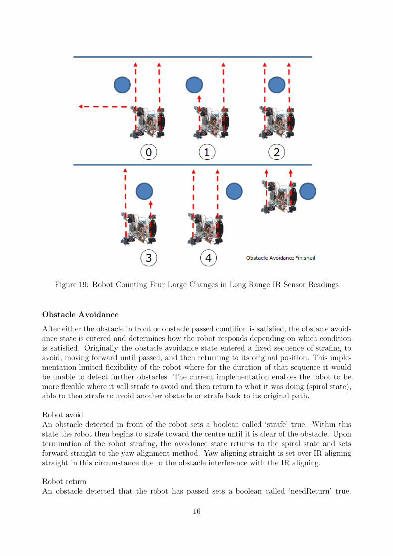
Figure 19: Robot Counting Four Large Changes in Long Range IR Sensor Readings

Obstacle Avoidance

After either the obstacle in front or obstacle passed condition is satisfied, the obstacle avoid-ance state is entered and determines how the robot responds depending on which conditionis satisfied. Originally the obstacle avoidance state entered a fixed sequence of strafing toavoid, moving forward until passed, and then returning to its original position. This imple-mentation limited flexibility of the robot where for the duration of that sequence it wouldbe unable to detect further obstacles. The current implementation enables the robot to bemore flexible where it will strafe to avoid and then return to what it was doing (spiral state),able to then strafe to avoid another obstacle or strafe back to its original path.

Robot avoidAn obstacle detected in front of the robot sets a boolean called ‘strafe’ true. Within thisstate the robot then begins to strafe toward the centre until it is clear of the obstacle. Upontermination of the robot strafing, the avoidance state returns to the spiral state and setsforward straight to the yaw alignment method. Yaw aligning straight is set over IR aligningstraight in this circumstance due to the obstacle interference with the IR aligning.

Robot returnAn obstacle detected that the robot has passed sets a boolean called ‘needReturn’ true.

16

Within this state the robot then begins to strafe toward the wall until the wall facing sensorsread values around the range of the starting reference. Upon satisfying this condition therobot has returned to its original distance for the spiral and returns to its spiral state.

Stopped

During spiraling, the length of the arena is measured, and the number of lengths requiredto cover the arena is calculated. Once this amount is reached, the robot stops - its run iscompleted.

5.3 Debugging Methods

For a project of this scale, testing is very important. As the Arduino environment doesn’thave very advanced debugging capabilities, the serial monitor and bluetooth were utilised.However the initial bluetooth receiver supplied was found to be faulty. This lead to relianceon bluetooth applications found on the Android app store. A large number of these appswere downloaded and tested, however the preferred application is ‘TerminalBT’, the userinterface for the app is shown in Figure 20. This meant that sensor readings and state in-formation of interest could be read out, allowing for easier identification of the source of aproblem.

Figure 20: Example Output being Read with TerminalBT

In the program written for this project there is a testing state where sections of code couldbe tested without running the entire program. This proved to be very useful for sensorcalibration/testing. Testing logic was a little more di�cult and usually required two stages.The first stage involves finding out where in the program an error is occurring. This is doneby printing lines that correspond to di↵erent stages in the code and sending them to thebluetooth module. The second stage involves working out why that particular section of codeisn’t working by sending all related sensor data to the bluetooth device, providing enoughinformation to work out what was going wrong.

17

6 Localisation & Mapping

6.1 LabVIEW

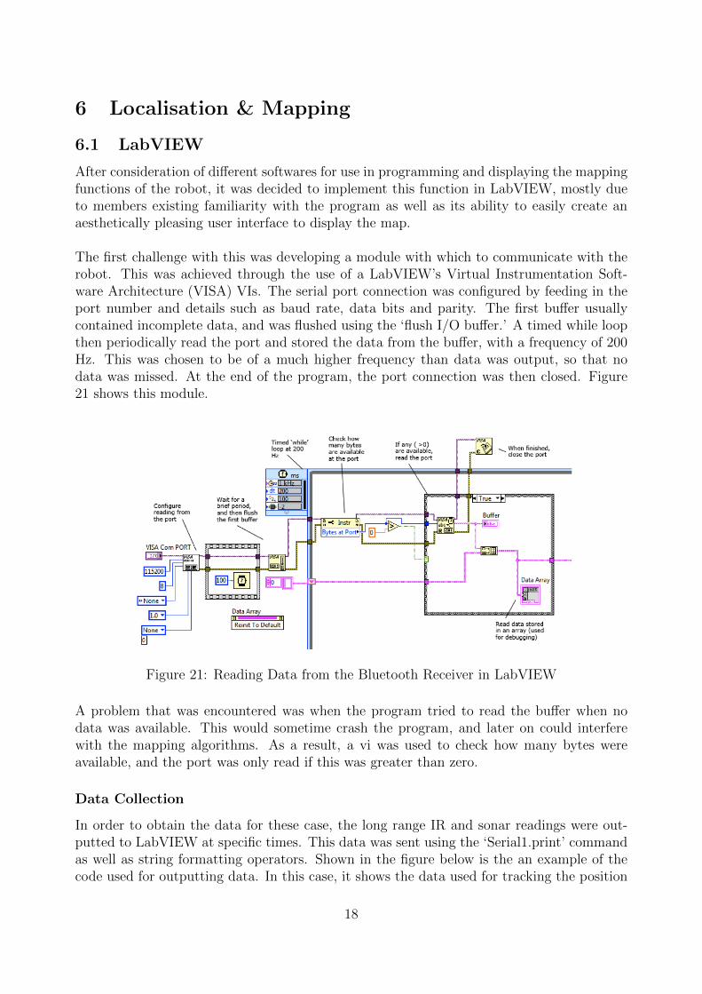
After consideration of di↵erent softwares for use in programming and displaying the mappingfunctions of the robot, it was decided to implement this function in LabVIEW, mostly dueto members existing familiarity with the program as well as its ability to easily create anaesthetically pleasing user interface to display the map.

The first challenge with this was developing a module with which to communicate with therobot. This was achieved through the use of a LabVIEW’s Virtual Instrumentation Soft-ware Architecture (VISA) VIs. The serial port connection was configured by feeding in theport number and details such as baud rate, data bits and parity. The first bu↵er usuallycontained incomplete data, and was flushed using the ‘flush I/O bu↵er.’ A timed while loopthen periodically read the port and stored the data from the bu↵er, with a frequency of 200Hz. This was chosen to be of a much higher frequency than data was output, so that nodata was missed. At the end of the program, the port connection was then closed. Figure21 shows this module.

Figure 21: Reading Data from the Bluetooth Receiver in LabVIEW

A problem that was encountered was when the program tried to read the bu↵er when nodata was available. This would sometime crash the program, and later on could interferewith the mapping algorithms. As a result, a vi was used to check how many bytes wereavailable, and the port was only read if this was greater than zero.

Data Collection

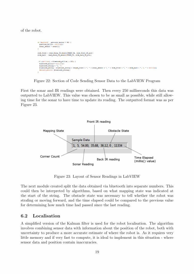
In order to obtain the data for these case, the long range IR and sonar readings were out-putted to LabVIEW at specific times. This data was sent using the ‘Serial1.print’ commandas well as string formatting operators. Shown in the figure below is the an example of thecode used for outputting data. In this case, it shows the data used for tracking the position

18

of the robot.

Figure 22: Section of Code Sending Sensor Data to the LabVIEW Program

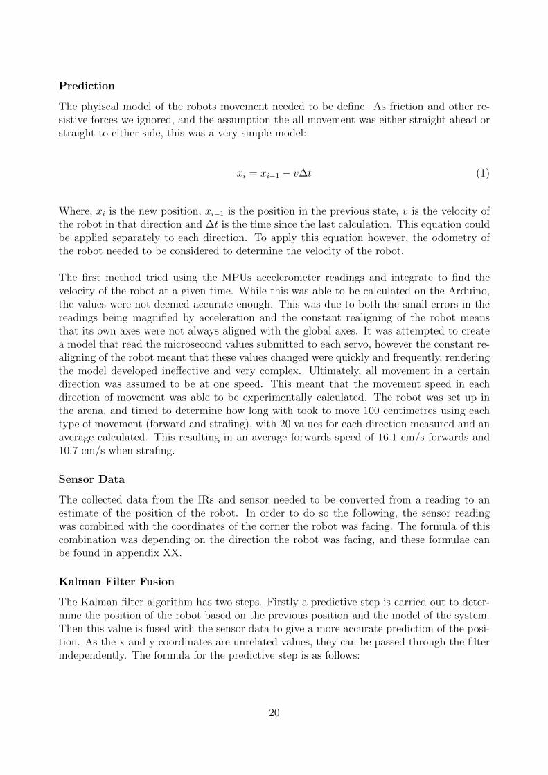
First the sonar and IR readings were obtained. Then every 250 milliseconds this data wasoutputted to LabVIEW. This value was chosen to be as small as possible, while still allow-ing time for the sonar to have time to update its reading. The outputted format was as perFigure 23.

Figure 23: Layout of Sensor Readings in LabVIEW

The next module created split the data obtained via bluetooth into separate numbers. Thiscould then be interpreted by algorithms, based on what mapping state was indicated atthe start of the string. The obstacle state was necessary to tell whether the robot wasstrafing or moving forward, and the time elapsed could be compared to the previous valuefor determining how much time had passed since the last reading.

6.2 Localisation

A simplified version of the Kalman filter is used for the robot localisation. The algorithminvolves combining sensor data with information about the position of the robot, both withuncertainty to produce a more accurate estimate of where the robot is. As it requires verylittle memory and if very fast to compute, it is ideal to implement in this situation - wheresensor data and position contain inaccuracies.

19

Prediction

The phyiscal model of the robots movement needed to be define. As friction and other re-sistive forces we ignored, and the assumption the all movement was either straight ahead orstraight to either side, this was a very simple model:

xi = xi�1 � v�t (1)

Where, xi is the new position, xi�1 is the position in the previous state, v is the velocity ofthe robot in that direction and �t is the time since the last calculation. This equation couldbe applied separately to each direction. To apply this equation however, the odometry ofthe robot needed to be considered to determine the velocity of the robot.

The first method tried using the MPUs accelerometer readings and integrate to find thevelocity of the robot at a given time. While this was able to be calculated on the Arduino,the values were not deemed accurate enough. This was due to both the small errors in thereadings being magnified by acceleration and the constant realigning of the robot meansthat its own axes were not always aligned with the global axes. It was attempted to createa model that read the microsecond values submitted to each servo, however the constant re-aligning of the robot meant that these values changed were quickly and frequently, renderingthe model developed ine↵ective and very complex. Ultimately, all movement in a certaindirection was assumed to be at one speed. This meant that the movement speed in eachdirection of movement was able to be experimentally calculated. The robot was set up inthe arena, and timed to determine how long with took to move 100 centimetres using eachtype of movement (forward and strafing), with 20 values for each direction measured and anaverage calculated. This resulting in an average forwards speed of 16.1 cm/s forwards and10.7 cm/s when strafing.

Sensor Data

The collected data from the IRs and sensor needed to be converted from a reading to anestimate of the position of the robot. In order to do so the following, the sensor readingwas combined with the coordinates of the corner the robot was facing. The formula of thiscombination was depending on the direction the robot was facing, and these formulae canbe found in appendix XX.

Kalman Filter Fusion

The Kalman filter algorithm has two steps. Firstly a predictive step is carried out to deter-mine the position of the robot based on the previous position and the model of the system.Then this value is fused with the sensor data to give a more accurate prediction of the posi-tion. As the x and y coordinates are unrelated values, they can be passed through the filterindependently. The formula for the predictive step is as follows:

20

yt|t�1 = Ftyt�1|t�1 +Btut (2)

Where y is the predicted y coordinate of position, t is the current time, t� 1 is the previoustime, Ft is the physical model to map the previous position to the new position, ut is thecontrol input and Bt is the conversion to map how this input a↵ects position. In this case,the filter is interested only in position, so all values are scalar. Taking the physical modelcalculated in equation 1, Ft is one, ut is v�t and Bt is also one, resulting in:

yt|t�1 = yt�1|t�1 + v�t (3)

The Kalman filter also estimates the uncertainty in the position estimate using a statevariance variable, P , which is also updated in the predictive state. The initial value of Pdepends on the accuracy of the system and was tuned to find an optimal value, in this casedetermined to be 0.5. The formula for calculating subsequent values is:

Pt|t�1 = FtPt�1|t�1FTt +Qt (4)

Qt represents the uncertainty in the system, due to uncontrolled external factors such aswind. In this case, it was assumed these factors had no e↵ect, as the car was inside andsheltered, allowing the formula to simplify to:

Pt|t�1 = Pt�1|t�1 (5)

The next step is to fuse in the values from the sensor using the following formula:

yt|t = yt|t�1 +Kt(Zt �Htyt|t�1) (6)

In this case Kt is the Kalman gain. This can be calculated using further formula, shownin equation 8. Zt is the sensor measurement, Ht is a value to map the predicted value tothe same scale as the measurements, in this case, one as both values are in centimetres andy is the value taken from the predicted step. The state variance is also updated from itspredicted value using the formula:

Pt|t = Pt|t�1 �KtHtPt|t�1 (7)

Finally the Kalman gain is calculated:

Kt = Pt|t�1HTt (HtPt|t�1H

Tt +Rt)

�1 (8)

21

Rt is the uncertainty associated with the measurement readings. This was also tuned ex-perimentally, and found to be zero for sonar readings and 0.4 for the long range IR sensors.These five formulae are continuously updated for both x and y at a frequency of 200 Hz totrack and calculate the robots path.

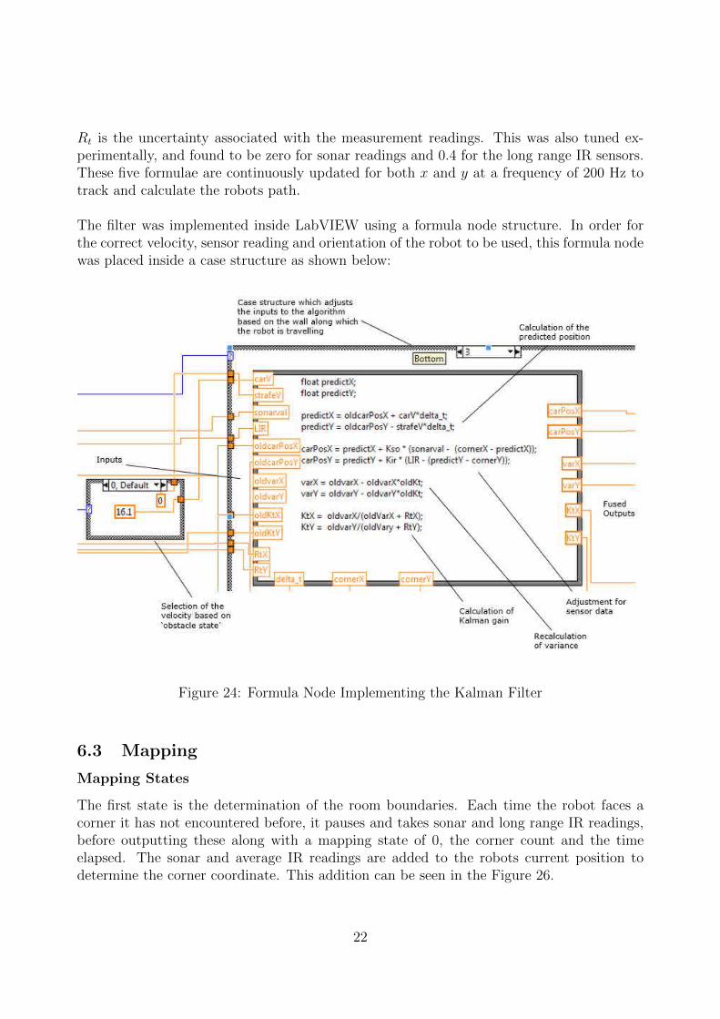
The filter was implemented inside LabVIEW using a formula node structure. In order forthe correct velocity, sensor reading and orientation of the robot to be used, this formula nodewas placed inside a case structure as shown below:

Figure 24: Formula Node Implementing the Kalman Filter

6.3 Mapping

Mapping States

The first state is the determination of the room boundaries. Each time the robot faces acorner it has not encountered before, it pauses and takes sonar and long range IR readings,before outputting these along with a mapping state of 0, the corner count and the timeelapsed. The sonar and average IR readings are added to the robots current position todetermine the corner coordinate. This addition can be seen in the Figure 26.

22

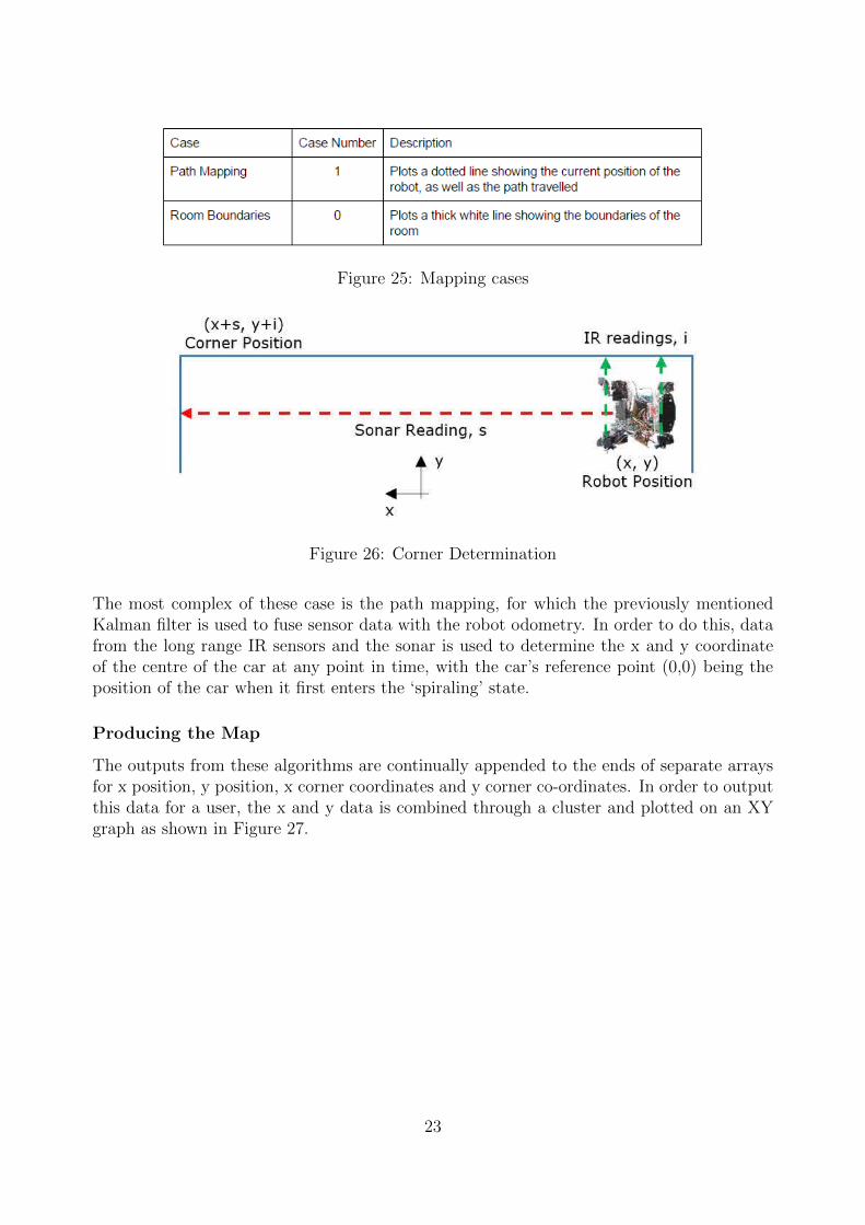
Figure 25: Mapping cases

Figure 26: Corner Determination

The most complex of these case is the path mapping, for which the previously mentionedKalman filter is used to fuse sensor data with the robot odometry. In order to do this, datafrom the long range IR sensors and the sonar is used to determine the x and y coordinateof the centre of the car at any point in time, with the car’s reference point (0,0) being theposition of the car when it first enters the ‘spiraling’ state.

Producing the Map

The outputs from these algorithms are continually appended to the ends of separate arraysfor x position, y position, x corner coordinates and y corner co-ordinates. In order to outputthis data for a user, the x and y data is combined through a cluster and plotted on an XYgraph as shown in Figure 27.

23

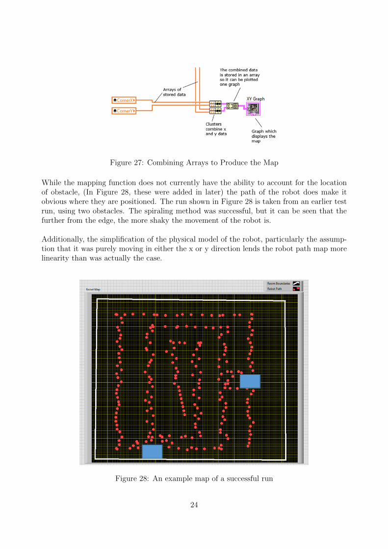
Figure 27: Combining Arrays to Produce the Map

While the mapping function does not currently have the ability to account for the locationof obstacle, (In Figure 28, these were added in later) the path of the robot does make itobvious where they are positioned. The run shown in Figure 28 is taken from an earlier testrun, using two obstacles. The spiraling method was successful, but it can be seen that thefurther from the edge, the more shaky the movement of the robot is.

Additionally, the simplification of the physical model of the robot, particularly the assump-tion that it was purely moving in either the x or y direction lends the robot path map morelinearity than was actually the case.

Figure 28: An example map of a successful run

24

Overall the map produced is successful at defining the boundaries of the room, as well asproviding a reasonably accurate live portrayal of the path it is taking. Additionally the liveplotting nature of the map meant that with some further work, interpretation of the mapcould have been used to send information back to the robot, allowing for full SLAM to beperformed.

7 Results

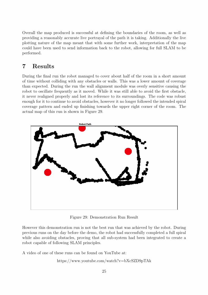
During the final run the robot managed to cover about half of the room in a short amountof time without colliding with any obstacles or walls. This was a lower amount of coveragethan expected. During the run the wall alignment module was overly sensitive causing therobot to oscillate frequently as it moved. While it was still able to avoid the first obstacle,it never realigned properly and lost its reference to its surroundings. The code was robustenough for it to continue to avoid obstacles, however it no longer followed the intended spiralcoverage pattern and ended up finishing towards the upper right corner of the room. Theactual map of this run is shown in Figure 29.

Figure 29: Demonstration Run Result

However this demonstration run is not the best run that was achieved by the robot. Duringprevious runs on the day before the demo, the robot had successfully completed a full spiralwhile also avoiding obstacles, proving that all sub-system had been integrated to create arobot capable of following SLAM principles.

A video of one of these runs can be found on YouTube at:

https://www.youtube.com/watch?v=bXcSZD9pTAk

25

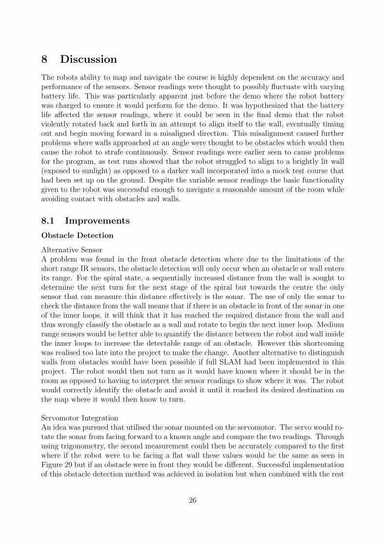
8 Discussion

The robots ability to map and navigate the course is highly dependent on the accuracy andperformance of the sensors. Sensor readings were thought to possibly fluctuate with varyingbattery life. This was particularly apparent just before the demo where the robot batterywas charged to ensure it would perform for the demo. It was hypothesized that the batterylife a↵ected the sensor readings, where it could be seen in the final demo that the robotviolently rotated back and forth in an attempt to align itself to the wall, eventually timingout and begin moving forward in a misaligned direction. This misalignment caused furtherproblems where walls approached at an angle were thought to be obstacles which would thencause the robot to strafe continuously. Sensor readings were earlier seen to cause problemsfor the program, as test runs showed that the robot struggled to align to a brightly lit wall(exposed to sunlight) as opposed to a darker wall incorporated into a mock test course thathad been set up on the ground. Despite the variable sensor readings the basic functionalitygiven to the robot was successful enough to navigate a reasonable amount of the room whileavoiding contact with obstacles and walls.

8.1 Improvements

Obstacle Detection

Alternative SensorA problem was found in the front obstacle detection where due to the limitations of theshort range IR sensors, the obstacle detection will only occur when an obstacle or wall entersits range. For the spiral state, a sequentially increased distance from the wall is sought todetermine the next turn for the next stage of the spiral but towards the centre the onlysensor that can measure this distance e↵ectively is the sonar. The use of only the sonar tocheck the distance from the wall means that if there is an obstacle in front of the sonar in oneof the inner loops, it will think that it has reached the required distance from the wall andthus wrongly classify the obstacle as a wall and rotate to begin the next inner loop. Mediumrange sensors would be better able to quantify the distance between the robot and wall insidethe inner loops to increase the detectable range of an obstacle. However this shortcomingwas realised too late into the project to make the change. Another alternative to distinguishwalls from obstacles would have been possible if full SLAM had been implemented in thisproject. The robot would then not turn as it would have known where it should be in theroom as opposed to having to interpret the sensor readings to show where it was. The robotwould correctly identify the obstacle and avoid it until it reached its desired destination onthe map where it would then know to turn.

Servomotor IntegrationAn idea was pursued that utilised the sonar mounted on the servomotor. The servo would ro-tate the sonar from facing forward to a known angle and compare the two readings. Throughusing trigonometry, the second measurement could then be accurately compared to the firstwhere if the robot were to be facing a flat wall these values would be the same as seen inFigure 29 but if an obstacle were in front they would be di↵erent. Successful implementationof this obstacle detection method was achieved in isolation but when combined with the rest

26

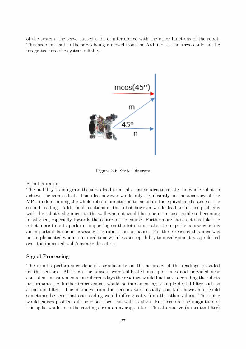
of the system, the servo caused a lot of interference with the other functions of the robot.This problem lead to the servo being removed from the Arduino, as the servo could not beintegrated into the system reliably.

Figure 30: State Diagram

Robot RotationThe inability to integrate the servo lead to an alternative idea to rotate the whole robot toachieve the same e↵ect. This idea however would rely significantly on the accuracy of theMPU in determining the whole robot’s orientation to calculate the equivalent distance of thesecond reading. Additional rotations of the robot however would lead to further problemswith the robot’s alignment to the wall where it would become more susceptible to becomingmisaligned, especially towards the centre of the course. Furthermore these actions take therobot more time to perform, impacting on the total time taken to map the course which isan important factor in assessing the robot’s performance. For these reasons this idea wasnot implemented where a reduced time with less susceptibility to misalignment was preferredover the improved wall/obstacle detection.

Signal Processing

The robot’s performance depends significantly on the accuracy of the readings providedby the sensors. Although the sensors were calibrated multiple times and provided nearconsistent measurements, on di↵erent days the readings would fluctuate, degrading the robotsperformance. A further improvement would be implementing a simple digital filter such asa median filter. The readings from the sensors were usually constant however it couldsometimes be seen that one reading would di↵er greatly from the other values. This spikewould causes problems if the robot used this wall to align. Furthermore the magnitude ofthis spike would bias the readings from an average filter. The alternative (a median filter)

27

would be far more e�cient in reducing this problem and the implementation of a digitalfilter would have produced a more consistent performance.

9 Conclusion

The solution presented in this report is an e↵ective implementation of SLAM principleswhich would allow the system to be used for an autonomous vacuum cleaner. The finalresult integrates four calibrated infra-sensors, two short range and two long range, an ultra-sonic ranging module and an MPU-9150, of which 6 degrees of freedom were used. Thisdesign enables proportional control of alignment with the wall regardless of facing, as wellas precise rotation control. These are combined to enable the robot to spiral inwards whilecovering the room. The short ranged IRs and the sonar also combined for complete coverageof the front of the robot, resulting in a obstacle collision rate of zero. Accurate live mappingis also a feature, with a LabVIEW implemented Kalman filter using sonar and long rangeIR readings to plot the robots path.

Improvements are still possible however, particularly with respect to the di↵erentiation ofobstacles and wall and a more comprehensive tuning method for the control system usedto align with walls. Further work on improving the reliability of the sensors for di↵eringamounts of ambient lights and battery levels would be particularly beneficial to improvingthe resilience of the design.

Ultimately, an autonomous robot capable of navigating the room and producing a satisfac-tory map has been created. During demonstration all obstacle were successfully avoided,with an approximate time of one and a half minutes. The coverage achieved was disappoint-ing however, mainly as a result of the robots inability to properly align to the wall and thusmaintain a consistent heading.

28

References

[1] Lemus R., Diaz S., Gutierrez C., Rodriguez D., Escobar F. (2014) SLAM-R Algorithm ofSimultaneous Localization and Mapping Using RFID for Obstacle Location and Recognition.Journal of Applied Research and Technology, Vol. 12 (3), p. 551 - 559

29

Appendices

Software Code

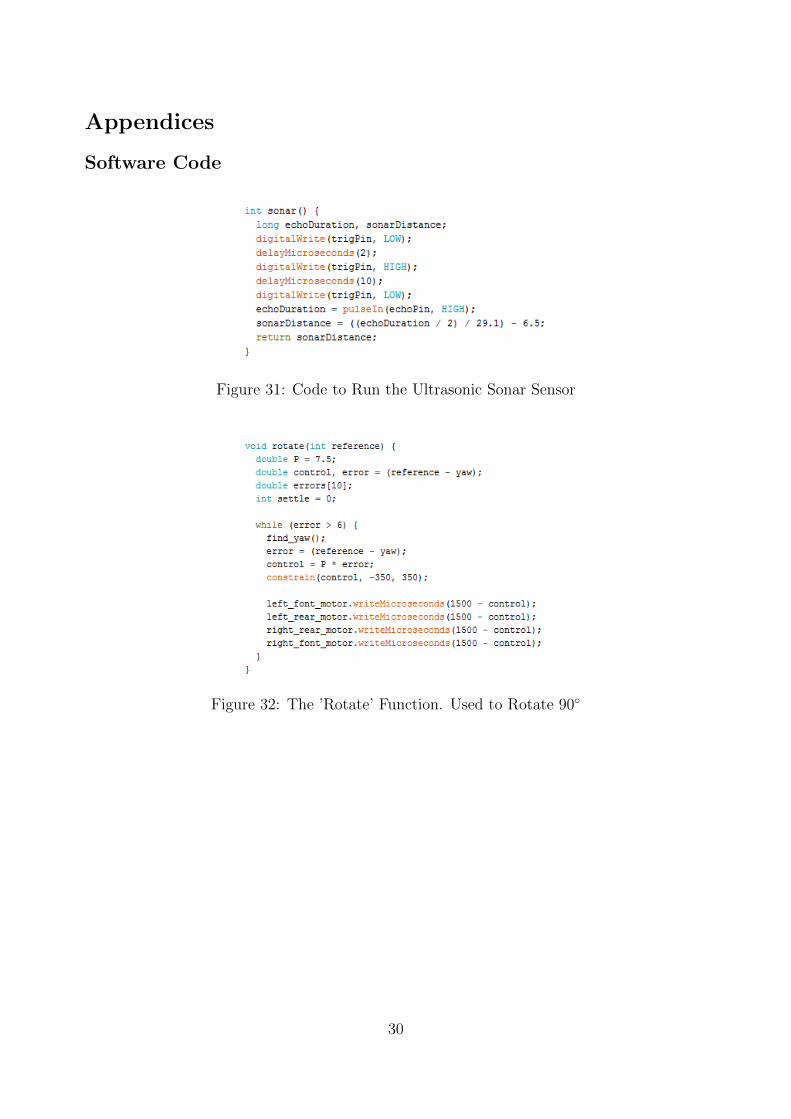
Figure 31: Code to Run the Ultrasonic Sonar Sensor

Figure 32: The ’Rotate’ Function. Used to Rotate 90�

30

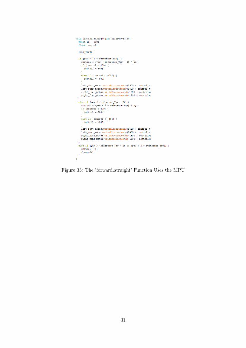
Figure 33: The ’forward straight’ Function Uses the MPU

31

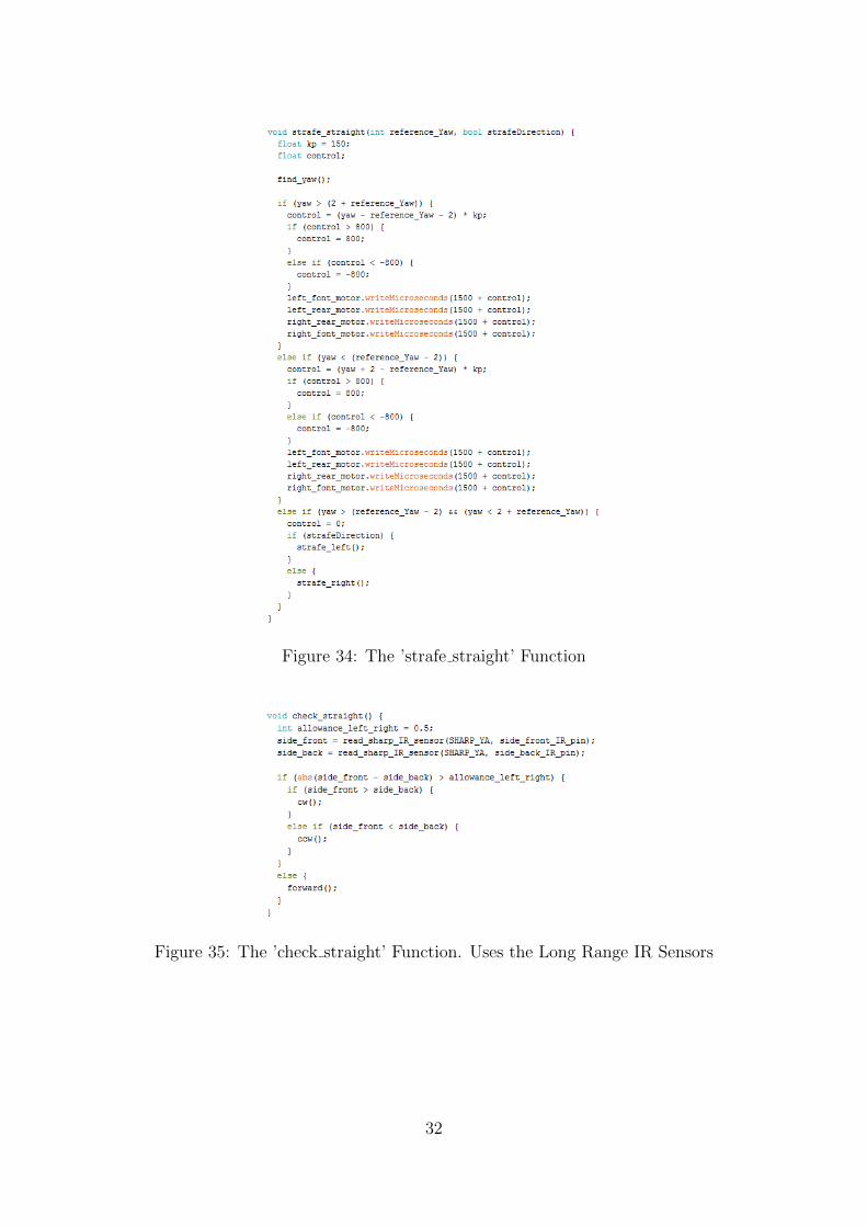
Figure 34: The ’strafe straight’ Function

Figure 35: The ’check straight’ Function. Uses the Long Range IR Sensors

32

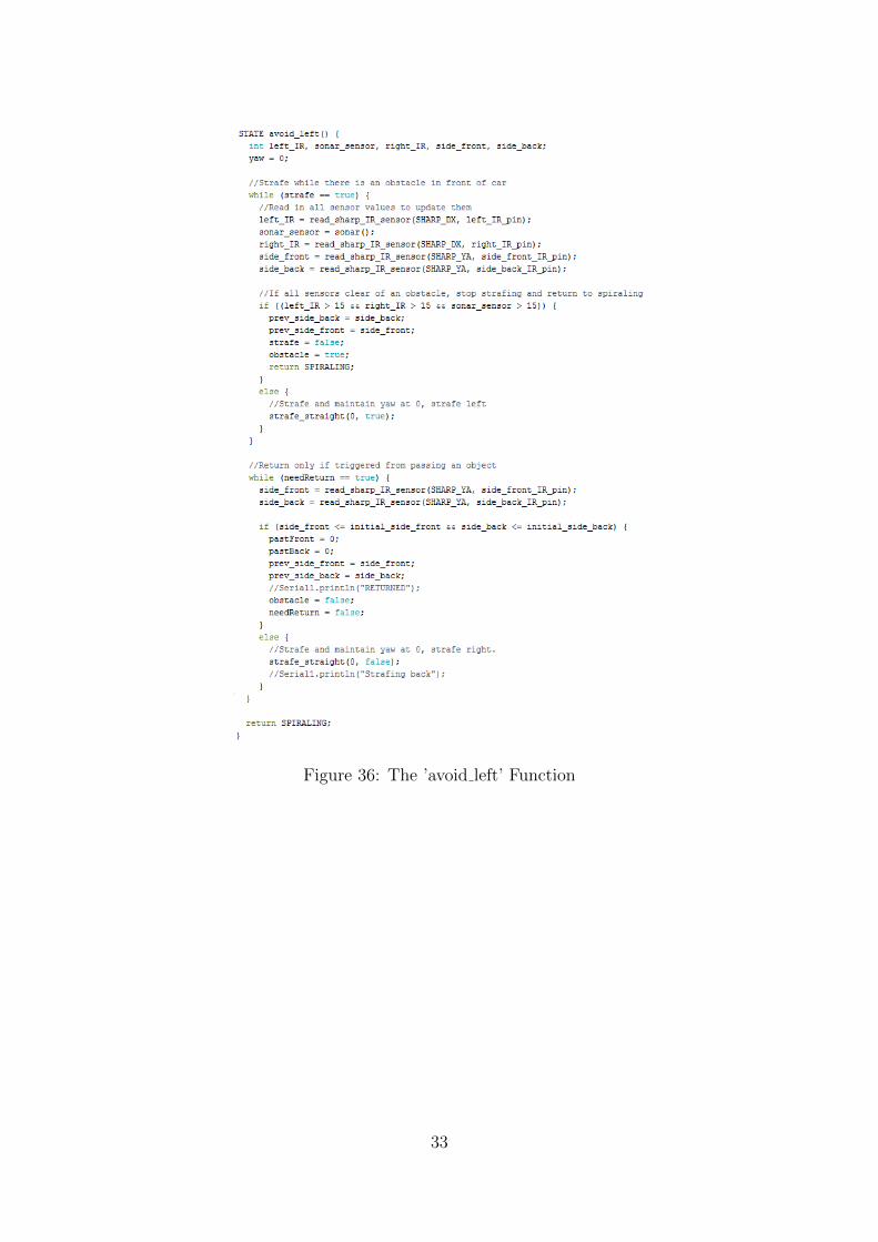
Figure 36: The ’avoid left’ Function

33

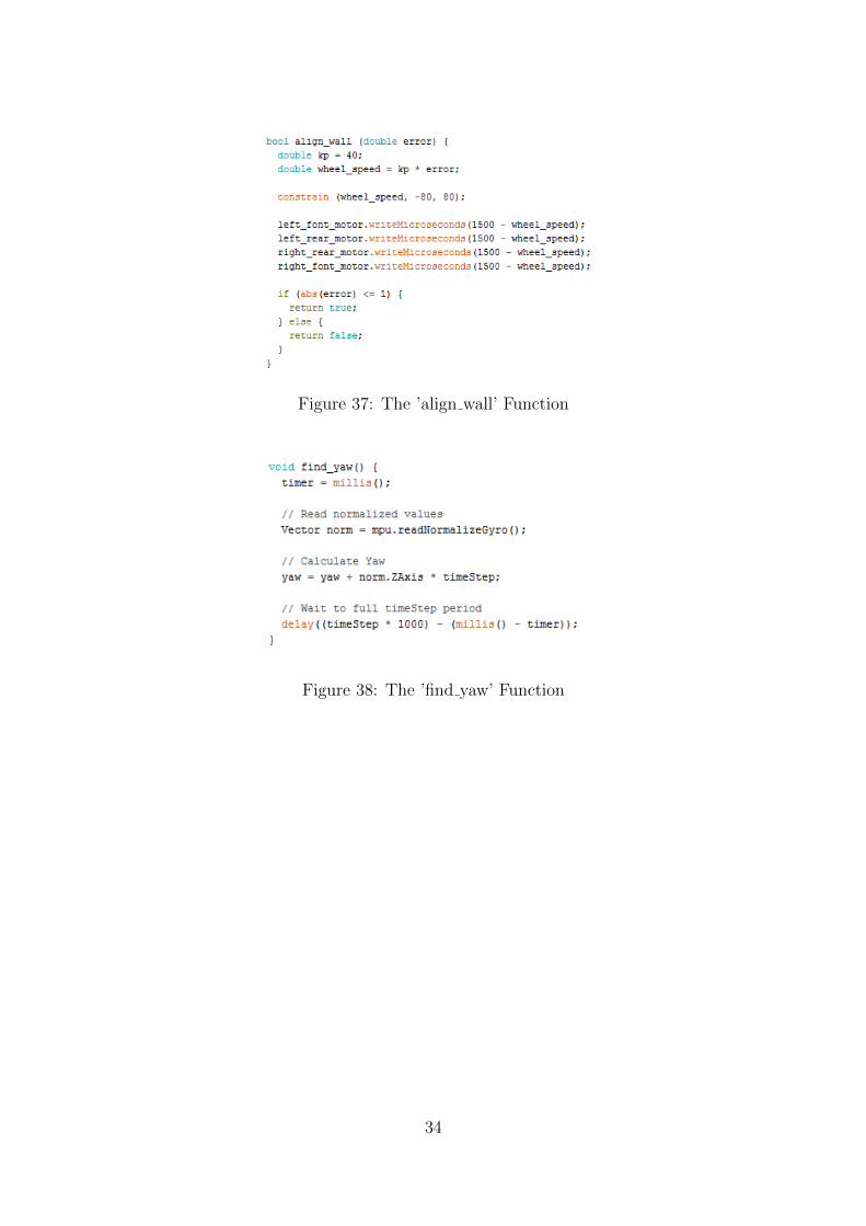
Figure 37: The ’align wall’ Function

Figure 38: The ’find yaw’ Function

34

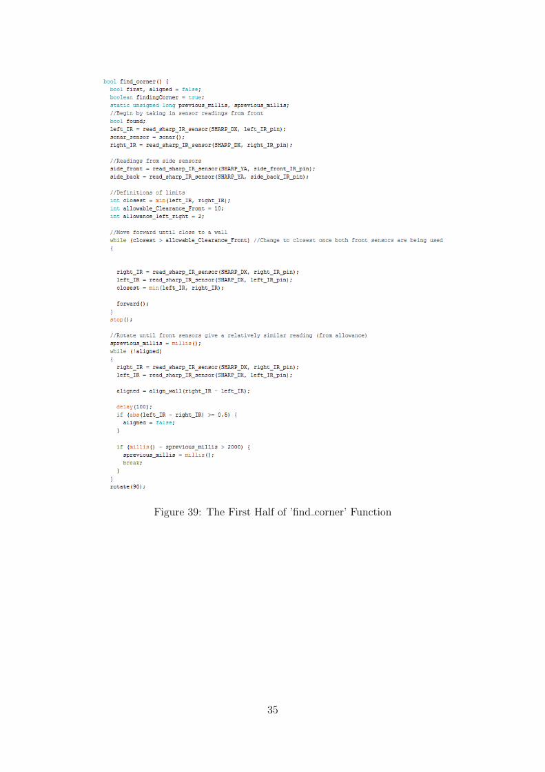
Figure 39: The First Half of ’find corner’ Function

35

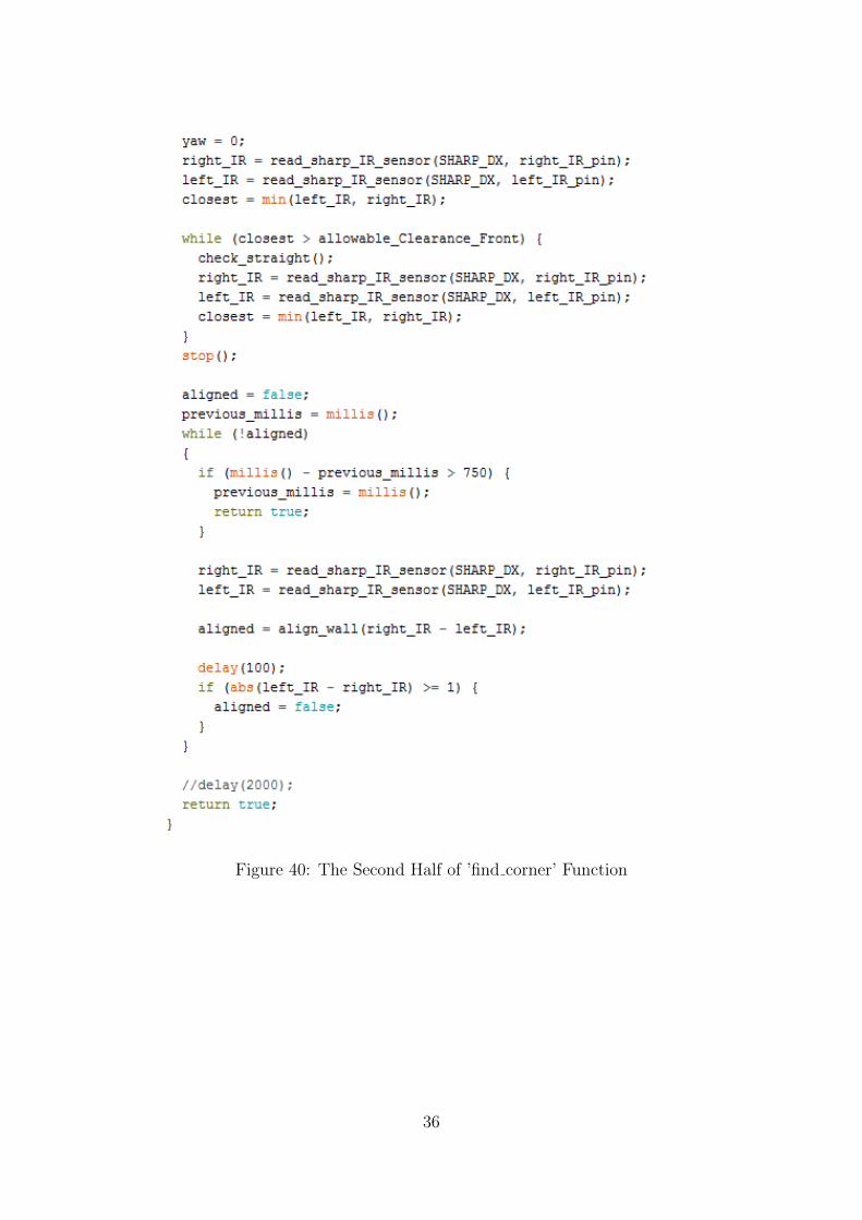
Figure 40: The Second Half of ’find corner’ Function

36

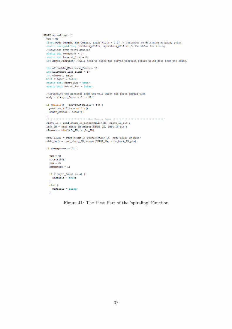
Figure 41: The First Part of the ’spiraling’ Function

37

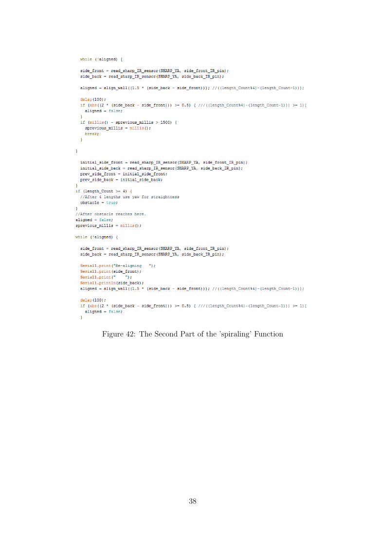
Figure 42: The Second Part of the ’spiraling’ Function

38

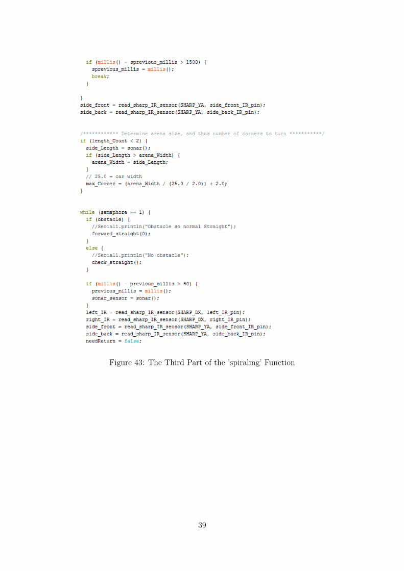
Figure 43: The Third Part of the ’spiraling’ Function

39

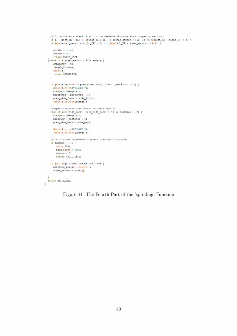
Figure 44: The Fourth Part of the ’spiraling’ Function

40

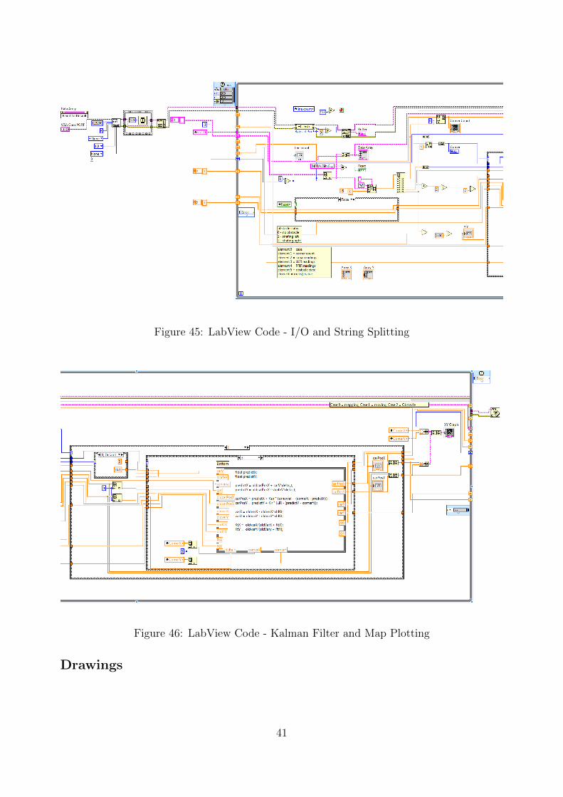
Figure 45: LabView Code - I/O and String Splitting

Figure 46: LabView Code - Kalman Filter and Map Plotting

Drawings

41

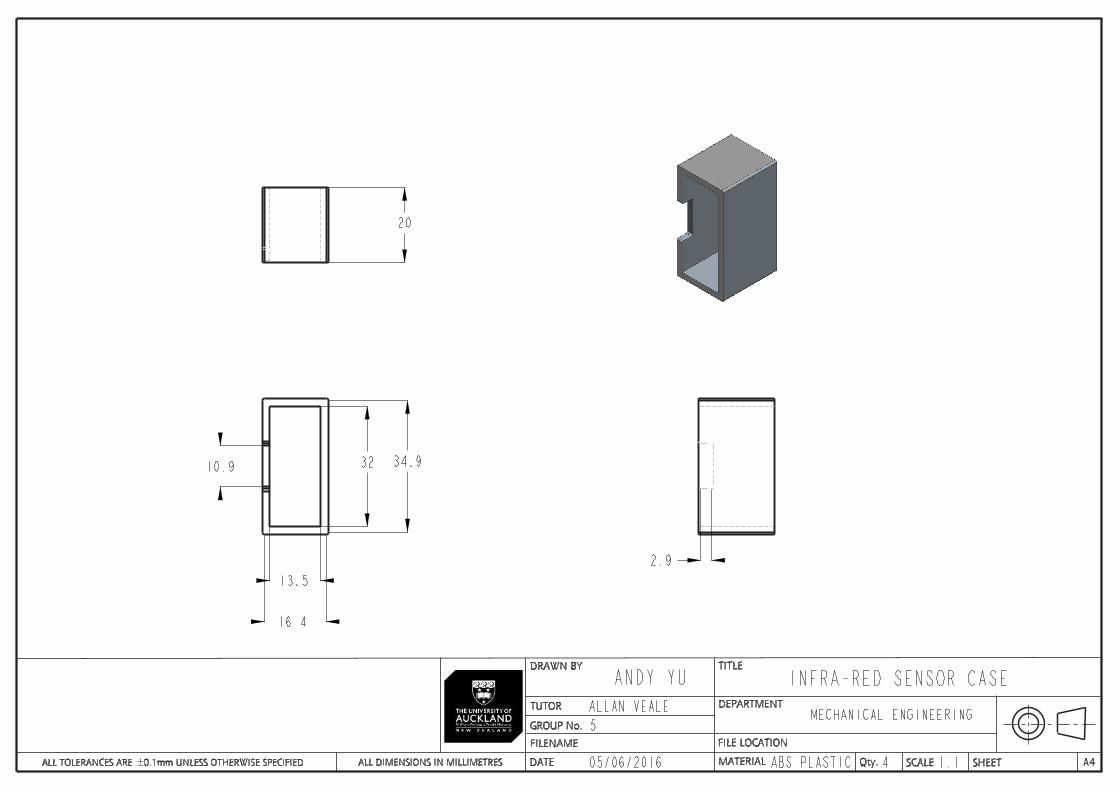
DRAWN BY

TUTOR

DATE SCALEALL DIMENSIONS IN MILLIMETRES

TITLE

A4SHEETQty.

GROUP No.

ALL TOLERANCES ARE 0.1mm UNLESS OTHERWISE SPECIFIED MATERIAL

DEPARTMENT

FILE LOCATIONFILENAME

13.5

16.4

34.93210.9

20

2.9

ANDY YU INFRA-RED SENSOR CASE

MECHANICAL ENGINEERINGALLAN VEALE5

05/06/2016 ABS PLASTIC 4 1:1

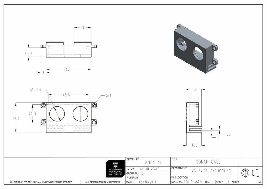
DRAWN BY

TUTOR

DATE SCALEALL DIMENSIONS IN MILLIMETRES

TITLE

A4SHEETQty.

GROUP No.

ALL TOLERANCES ARE 0.1mm UNLESS OTHERWISE SPECIFIED MATERIAL

DEPARTMENT

FILE LOCATIONFILENAME

50

19

10.5

6

16.5

4

33.5

1.51

13

16.5

20.5

45.5

ANDY YU SONAR CASE

MECHANICAL ENGINEERING

05/06/2016

5ALLAN VEALE

ABS PLASTIC 1 1:!

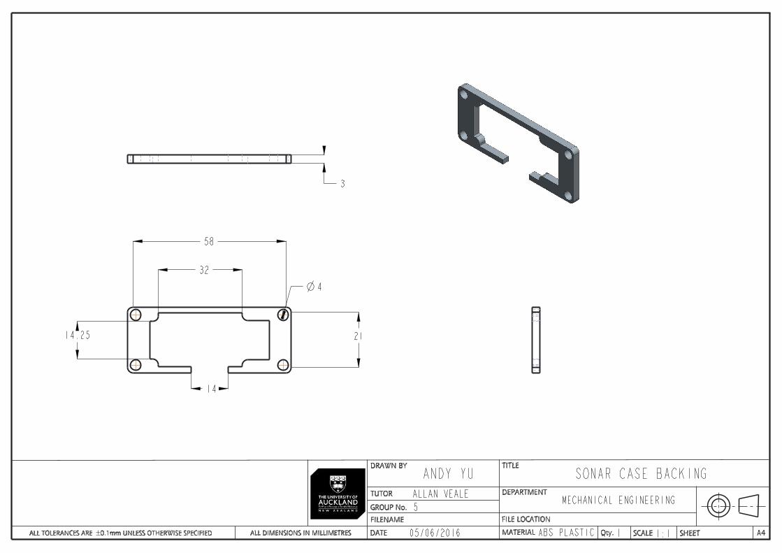
DRAWN BY

TUTOR

DATE SCALEALL DIMENSIONS IN MILLIMETRES

TITLE

A4SHEETQty.

GROUP No.

ALL TOLERANCES ARE 0.1mm UNLESS OTHERWISE SPECIFIED MATERIAL

DEPARTMENT

FILE LOCATIONFILENAME

4

21

58

14.25

14

3

32

SONAR CASE BACKINGANDY YUALLAN VEALE5

05/06/2016 ABS PLASTIC 1 1:1

MECHANICAL ENGINEERING

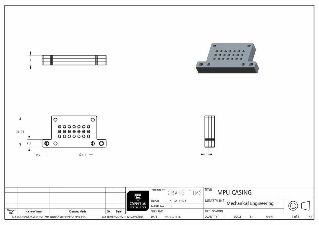
DRAWN BY

TUTOR

DATE SCALEALL DIMENSIONS IN MILLIMETRES

TITLE

A4SHEETQUANTITY

GROUP No.

ALL TOLERANCES ARE 0.1mm UNLESS OTHERWISE SPECIFIED

DEPARTMENT

FILE LOCATIONFILENAME

29.24

7.1

9

33.14

Change No. Name of Item Changes Made OK Date

MPU CASING

Mechanical Engineering

1 1 : 1 1 of 1

CRAIG TIMSALLAN VEALE

5

05/06/2016