Embed Size (px)
Citation preview
Autonomous Mobile RobotsCPE 470/670
Lecture 6
Instructor: Monica Nicolescu
CPE 470/670 - Lecture 6 2
Review
Sensors
• Reflective optosensors
• Infrared sensors
• Break-Beam sensors
• Shaft encoders
• Ultrasonic sensors
• Laser sensing
• Visual sensing
CPE 470/670 - Lecture 6 3
Vision from Motion
• Take advantage of motion to facilitate vision
• Static system can detect moving objects
– Subtract two consecutive images from each other the
movement between frames
• Moving system can detect static objects
– At consecutive time steps continuous objects move as one
– Exact movement of the camera should be known
• Robots are typically moving themselves
– Need to consider the movement of the robot
CPE 470/670 - Lecture 6 4
Stereo Vision
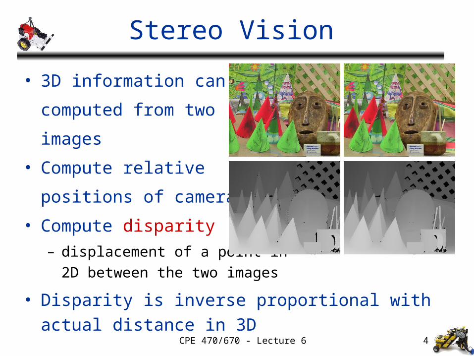
• 3D information can be
computed from two
images
• Compute relative
positions of cameras
• Compute disparity
– displacement of a point in
2D between the two images
• Disparity is inverse proportional with actual distance
in 3D
CPE 470/670 - Lecture 6 5
Biological Vision
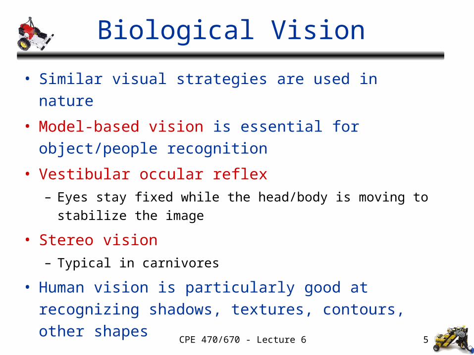
• Similar visual strategies are used in nature
• Model-based vision is essential for object/people
recognition
• Vestibular occular reflex– Eyes stay fixed while the head/body is moving to stabilize
the image
• Stereo vision– Typical in carnivores
• Human vision is particularly good at recognizing
shadows, textures, contours, other shapes
CPE 470/670 - Lecture 6 6
Vision for Robots
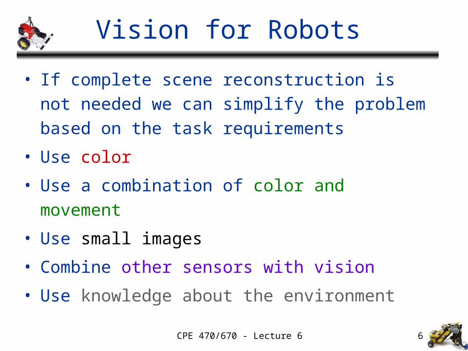
• If complete scene reconstruction is not needed we
can simplify the problem based on the task
requirements
• Use color
• Use a combination of color and movement
• Use small images
• Combine other sensors with vision
• Use knowledge about the environment
CPE 470/670 - Lecture 6 7
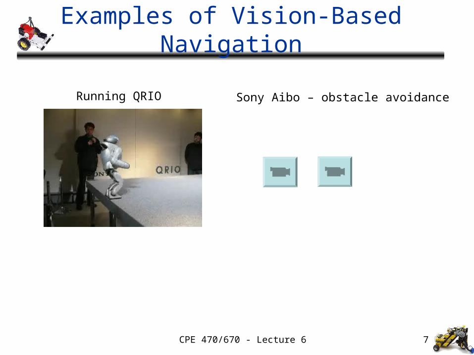
Examples of Vision-Based Navigation
Running QRIO Sony Aibo – obstacle avoidance
CPE 470/670 - Lecture 6 8
Feedback Control
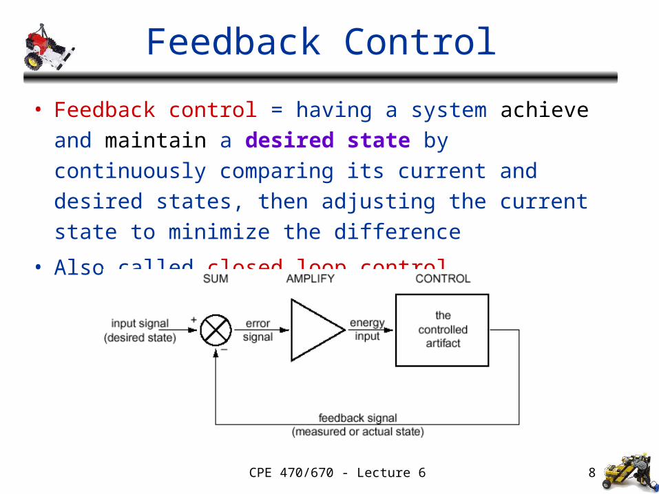
• Feedback control = having a system achieve and
maintain a desired state by continuously
comparing its current and desired states, then
adjusting the current state to minimize the difference
• Also called closed loop control
CPE 470/670 - Lecture 6 9
Goal State
• Goal driven behavior is used in both control theory
and in AI
• Goals in AI
– Achievement goals: states that the system is trying to
reach
– Maintenance goals: states that need to be maintained
• Control theory: mostly focused on maintenance goals
• Goal states can be:
– Internal: monitor battery power level
– External: get to a particular location in the environment
– Combinations of both: balance a pole
CPE 470/670 - Lecture 6 10
Error
• Error = the difference in the current state and desired state of
the system
• The controller has to minimize the error at all times
• Zero/non-zero error:
– Tells whether there is an error or not
– The least information we could have
• Magnitude of error:
– The distance to the goal state
• Direction of error:
– Which way to go to minimize the error
• Control is much easier if we know both magnitude and direction
CPE 470/670 - Lecture 6 11
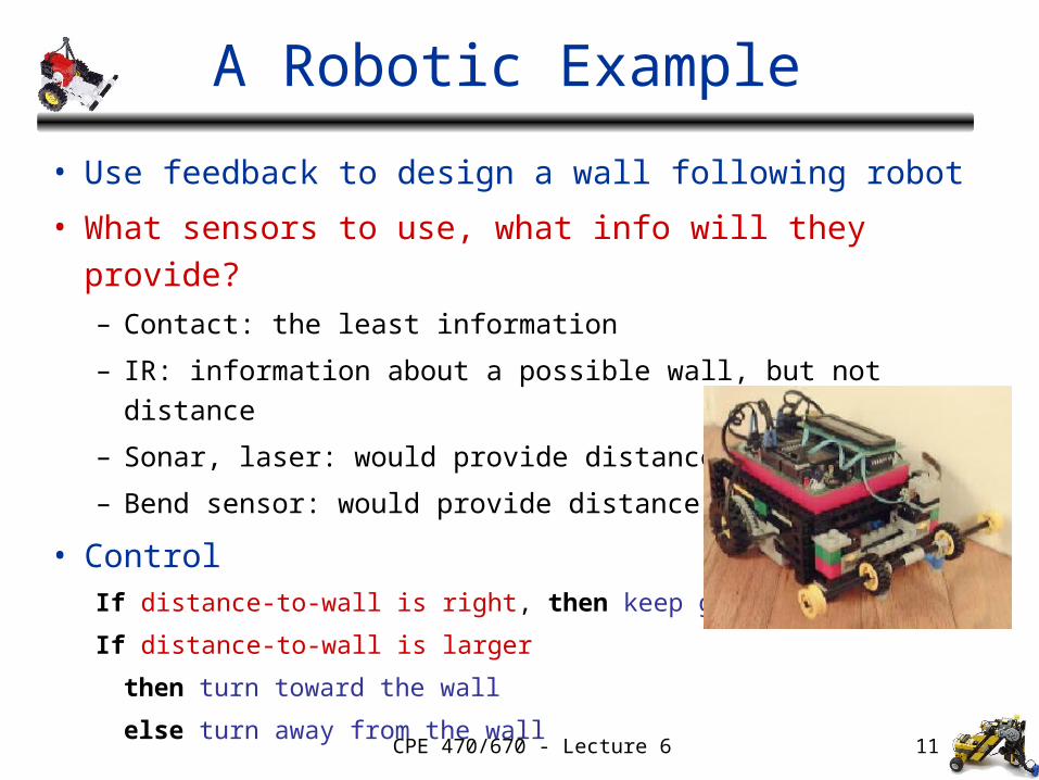
A Robotic Example
• Use feedback to design a wall following robot
• What sensors to use, what info will they provide?– Contact: the least information
– IR: information about a possible wall, but not distance
– Sonar, laser: would provide distance
– Bend sensor: would provide distance
• ControlIf distance-to-wall is right, then keep going
If distance-to-wall is larger
then turn toward the wall
else turn away from the wall
CPE 470/670 - Lecture 6 12
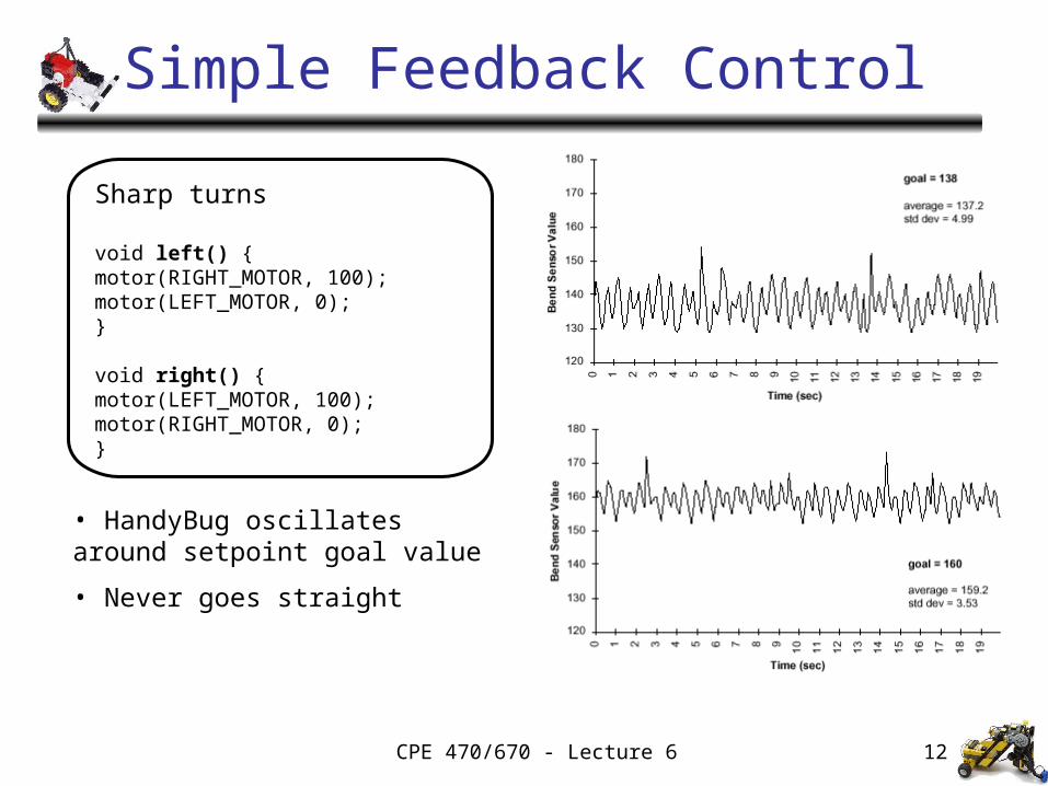
Simple Feedback Control
• HandyBug oscillates around setpoint goal value
• Never goes straight
Sharp turns
void left() {motor(RIGHT_MOTOR, 100);motor(LEFT_MOTOR, 0);}
void right() {motor(LEFT_MOTOR, 100);motor(RIGHT_MOTOR, 0);}
CPE 470/670 - Lecture 6 13
Overshoot
• The system goes beyond its setpoint changes
direction before stabilizing on it
• For this example overshoot is not a critical problem
• Other situations are more critical
– A robot arm moving to a particular position
– Going beyond the goal position could have collided with
some object just beyond the setpoint position
CPE 470/670 - Lecture 6 14
Oscillations
• The robot oscillates around the optimal distance
from the wall, getting either too close or too far
• In general, the behavior of a feedback system
oscillates around the desired state
• Decreasing oscillations
– Adjust the turning angle
– Use a range instead of a fixed distance as the goal state
CPE 470/670 - Lecture 6 15
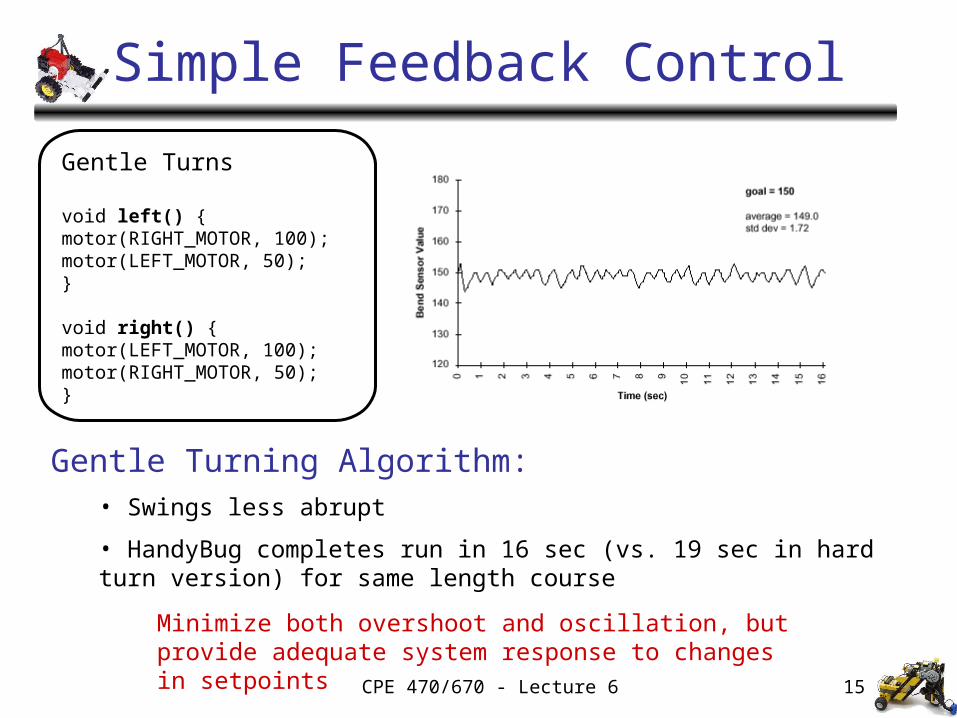
Simple Feedback Control
Gentle Turning Algorithm:• Swings less abrupt
• HandyBug completes run in 16 sec (vs. 19 sec in hard turn version) for same length course
Gentle Turns
void left() {motor(RIGHT_MOTOR, 100);motor(LEFT_MOTOR, 50);}
void right() {motor(LEFT_MOTOR, 100);motor(RIGHT_MOTOR, 50);}
Minimize both overshoot and oscillation, but provide adequate system response to changes in setpoints
CPE 470/670 - Lecture 6 16
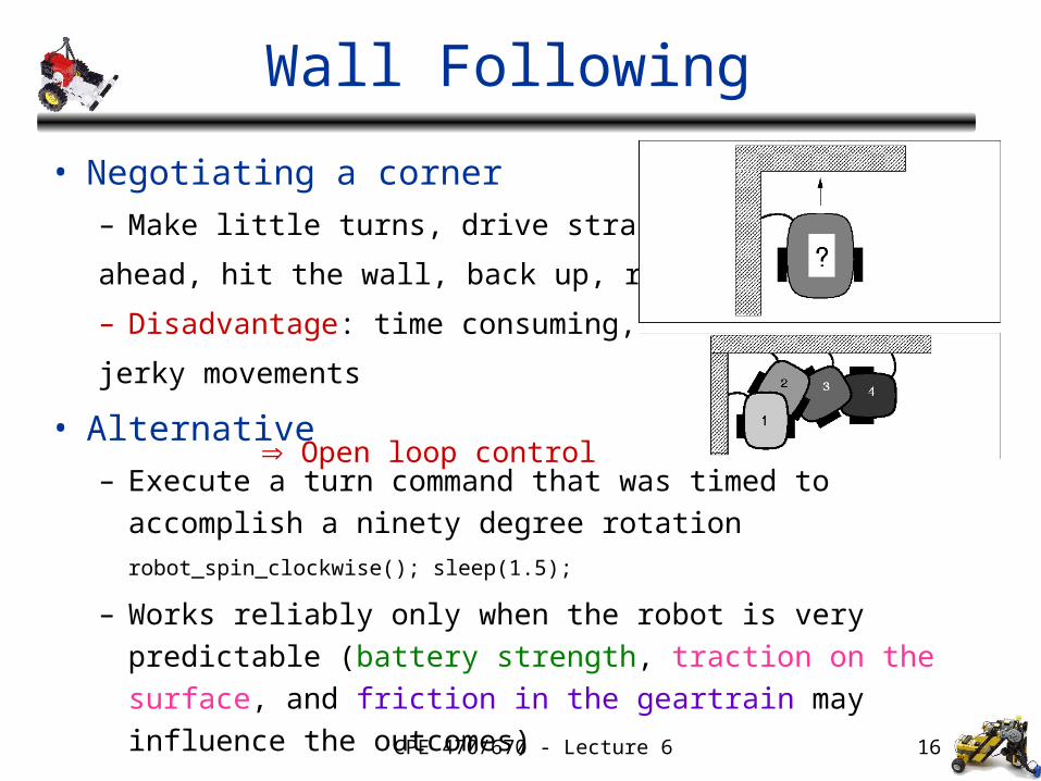
Wall Following
• Negotiating a corner
– Make little turns, drive straight
ahead, hit the wall, back up, repeat
– Disadvantage: time consuming,
jerky movements
• Alternative
– Execute a turn command that was timed to accomplish a
ninety degree rotation robot_spin_clockwise(); sleep(1.5);
– Works reliably only when the robot is very predictable
(battery strength, traction on the surface, and friction in the
geartrain may influence the outcomes)
Open loop control
CPE 470/670 - Lecture 6 17
Open Loop Control
• Does not use sensory feedback, and state is not fed back into the system
• Feed-forward control– The command signal is a function of some parameters
measured in advance
– E.g.: battery strength measurement could be used to "predict" how much time is needed for the turn
– Still open loop control, but a computation is made to make the control more accurate
• Feed-forward systems are effective only if– They are well calibrated
– The environment is predictable & does not change such as to affect their performance
CPE 470/670 - Lecture 6 18
Uses of Open Loop Control
• Repetitive, state independent tasks
– Switch microwave on to defrost for 2 minutes
– Program a toy robot to walk in a certain direction
– Switch a sprinkler system on to water the garden at set
times
– Conveyor belt machines

CPE 470/670 - Lecture 6 19
Types of Feedback Control
There are three types of basic feedback controllers
• P: proportional control
• PD: proportional derivative control
• PID: proportional integral derivative control
CPE 470/670 - Lecture 6 20
Proportional Control
• The response of the system is proportional to the amount of the error
• The output o is proportional to the input i:
o = Kp i
• Kp is a proportionality constant (gain)
• Control generates a stronger response the farther away the system is from the goal state
• Turn sharply toward the wall sharply if far from it,
• Turn gently toward the wall if slightly farther from it
CPE 470/670 - Lecture 6 21
Determining Gains
• How do we determine the gains?
• Empirically (trial and error):
– require that the system be tested extensively
• Analytically (mathematics):
– require that the system be well understood and
characterized mathematically
• Automatically
– by trying different values at run-time
CPE 470/670 - Lecture 6 22
Gains
• The gains (Kp) are specific to the particular control
system
– The physical properties of the system directly affect the
gain values
– E.g.: the velocity profile of a motor (how fast it can
accelerate and decelerate), the backlash and friction in the
gears, the friction on the surface, in the air, etc.
– All of these influence what the system actually does in
response to a command
CPE 470/670 - Lecture 6 23
Gains and Oscillations
• Incorrect gains will cause the system to undershoot or
overshoot the desired state oscillations
• Gain values determine if:
– The system will keep oscillating (possibly increasing
oscillations)
– The system will stabilize
• Damping: process of systematically decreasing oscillations
• A system is properly damped if it does not oscillate
out of control (decreasing oscillations, or no oscillations at
all)
CPE 470/670 - Lecture 6 24
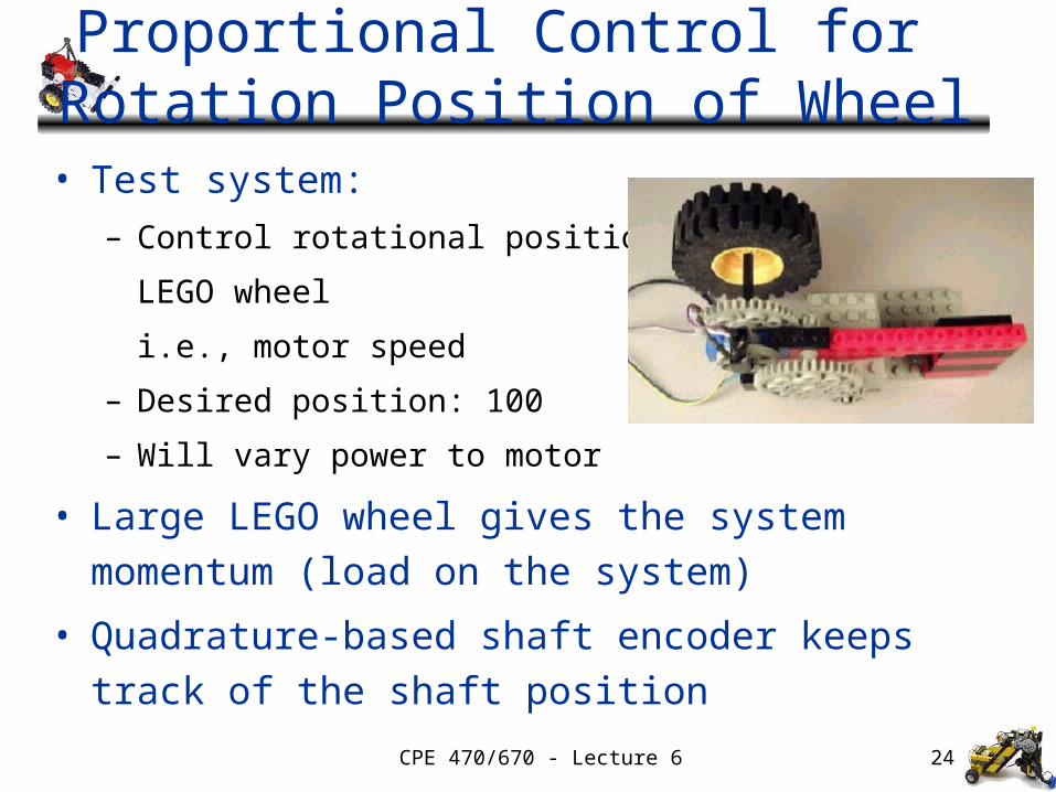
Proportional Control for Rotation Position of Wheel
• Test system:
– Control rotational position of
LEGO wheel
i.e., motor speed
– Desired position: 100
– Will vary power to motor
• Large LEGO wheel gives the system momentum
(load on the system)
• Quadrature-based shaft encoder keeps track of the
shaft position
CPE 470/670 - Lecture 6 25
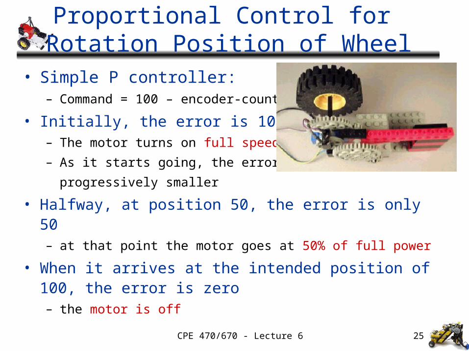
Proportional Control for Rotation Position of Wheel
• Simple P controller:– Command = 100 – encoder-counts
• Initially, the error is 100– The motor turns on full speed
– As it starts going, the error becomes
progressively smaller
• Halfway, at position 50, the error is only 50– at that point the motor goes at 50% of full power
• When it arrives at the intended position of 100, the error is zero– the motor is off
CPE 470/670 - Lecture 6 26
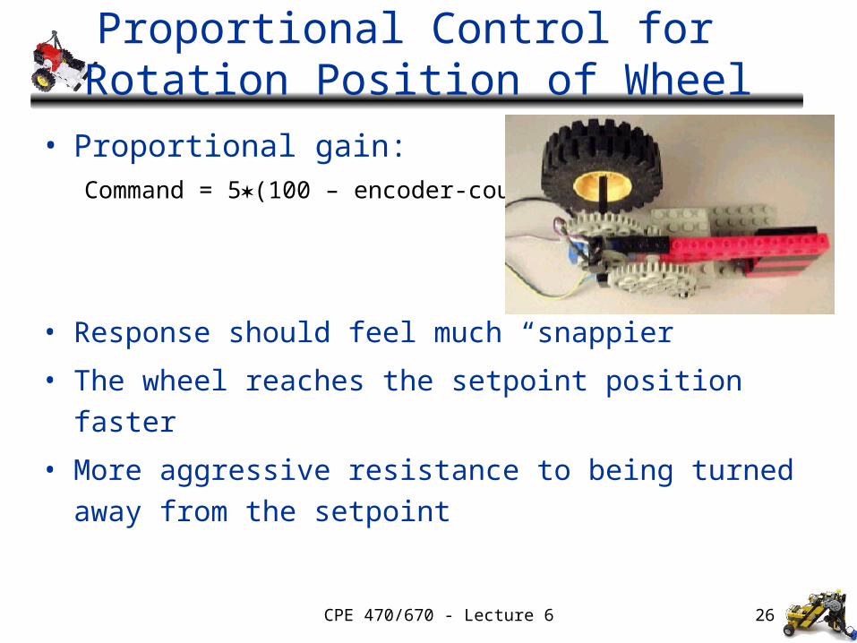
Proportional Control for Rotation Position of Wheel
• Proportional gain:Command = 5(100 – encoder-counts)
• Response should feel much “snappier”
• The wheel reaches the setpoint position faster
• More aggressive resistance to being turned away from
the setpoint
CPE 470/670 - Lecture 6 27
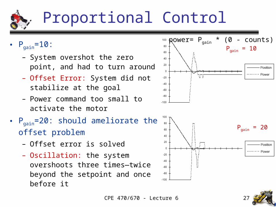
Proportional Control
• Pgain=10:
– System overshot the zero point, and had to turn around
– Offset Error: System did not stabilize at the goal
– Power command too small to activate the motor
• Pgain=20: should ameliorate the offset
problem– Offset error is solved
– Oscillation: the system overshoots three times—twice beyond the setpoint and once before it
Pgain = 10
Pgain = 20
power= Pgain * (0 - counts)
CPE 470/670 - Lecture 6 28
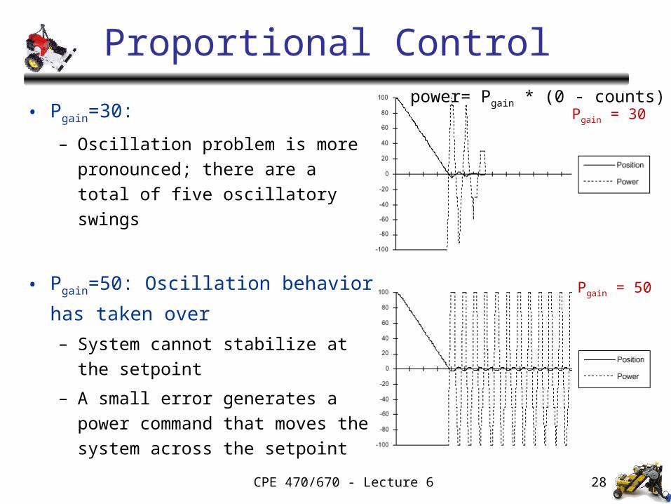
Proportional Control
• Pgain=30:
– Oscillation problem is more
pronounced; there are a total of five
oscillatory swings
• Pgain=50: Oscillation behavior has
taken over
– System cannot stabilize at the
setpoint
– A small error generates a power
command that moves the system
across the setpoint
Pgain = 30
Pgain = 50
power= Pgain * (0 - counts)
CPE 470/670 - Lecture 6 29
Derivative Control
• Setting gains is difficult, and simply increasing the
gains does not remove oscillations
• The system needs to be controlled differently
when it is close to the desired state and when it is far
from it
• The momentum of the correction carries the system
beyond the desired state, and causes oscillations
Momentum = mass velocity
• Solution: correct the momentum as the system
approaches the desired state
CPE 470/670 - Lecture 6 30
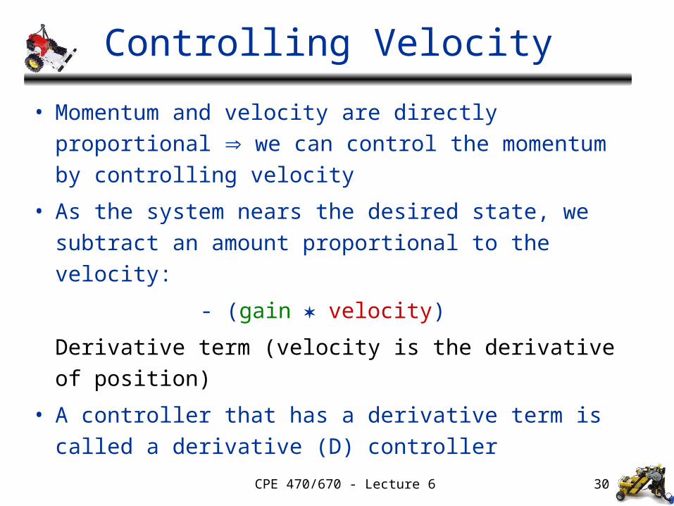
Controlling Velocity
• Momentum and velocity are directly proportional
we can control the momentum by controlling velocity
• As the system nears the desired state, we subtract
an amount proportional to the velocity:
- (gain velocity)
Derivative term (velocity is the derivative of position)
• A controller that has a derivative term is called a
derivative (D) controller
CPE 470/670 - Lecture 6 31
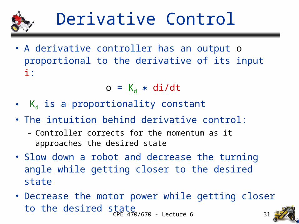
Derivative Control
• A derivative controller has an output o proportional to the derivative of its input i:
o = Kd di/dt
• Kd is a proportionality constant
• The intuition behind derivative control: – Controller corrects for the momentum as it approaches the
desired state
• Slow down a robot and decrease the turning angle while getting closer to the desired state
• Decrease the motor power while getting closer to the desired state
CPE 470/670 - Lecture 6 32
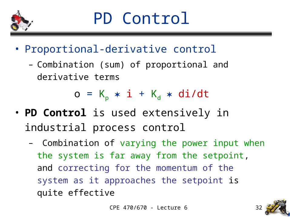
PD Control
• Proportional-derivative control
– Combination (sum) of proportional and derivative terms
o = Kp i + Kd di/dt
• PD Control is used extensively in industrial process
control
– Combination of varying the power input when the system is far away from the setpoint, and correcting for the momentum of the system as it approaches the setpoint is quite effective
CPE 470/670 - Lecture 6 33
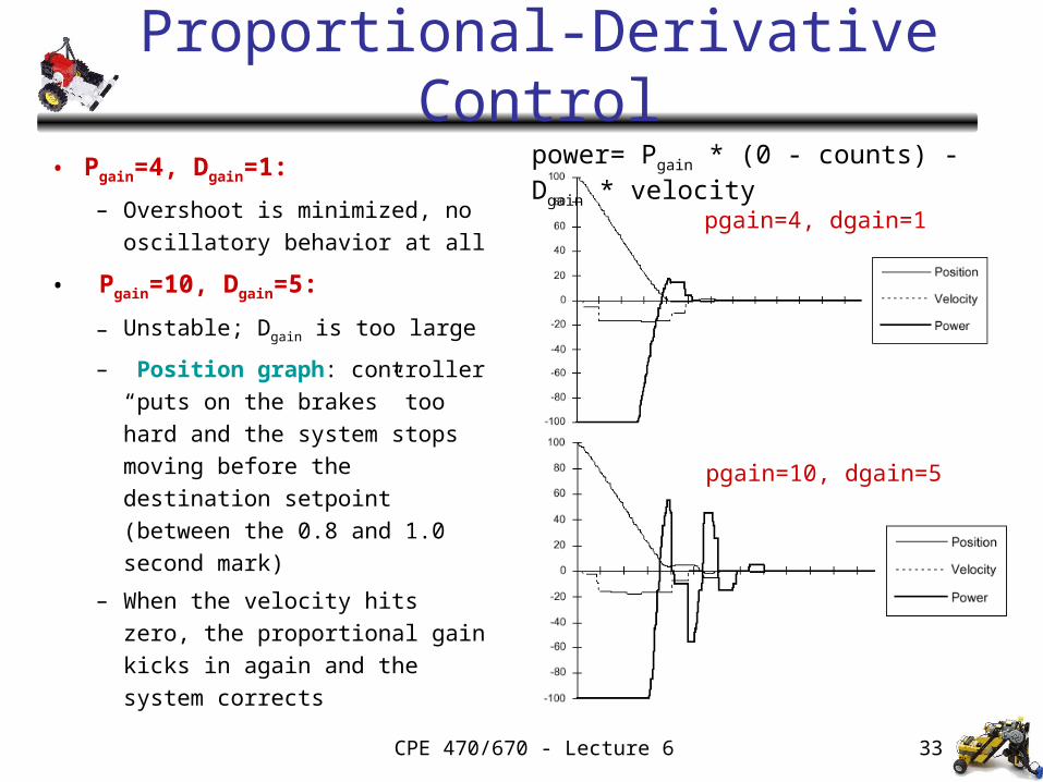
Proportional-Derivative Control
• Pgain=4, Dgain=1:
– Overshoot is minimized, no
oscillatory behavior at all
• Pgain=10, Dgain=5:
– Unstable; Dgain is too large
– Position graph: controller
“puts on the brakes” too hard
and the system stops moving
before the destination setpoint
(between the 0.8 and 1.0
second mark)
– When the velocity hits zero,
the proportional gain kicks in
again and the system corrects
pgain=4, dgain=1
pgain=10, dgain=5
power= Pgain * (0 - counts) - Dgain * velocity
CPE 470/670 - Lecture 6 34
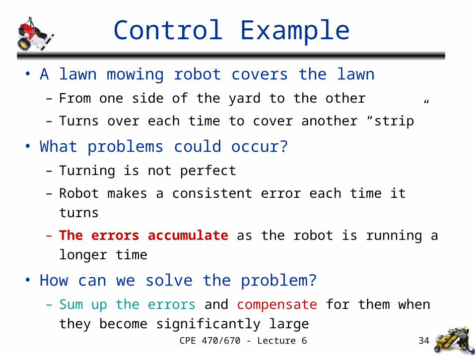
Control Example
• A lawn mowing robot covers the lawn
– From one side of the yard to the other
– Turns over each time to cover another “strip”
• What problems could occur?
– Turning is not perfect
– Robot makes a consistent error each time it turns
– The errors accumulate as the robot is running a
longer time
• How can we solve the problem?
– Sum up the errors and compensate for them when
they become significantly large

CPE 470/670 - Lecture 6 35
Integral Control
• Control system can be improved by introducing an
integral term
o = Kf i(t)dt
• Kf = proportionality constant
• Intuition:
– System keeps track of its repeatable, steady state errors
– These errors are integrated (summed up) over time
– When they reach a threshold, the system compensates for
them
CPE 470/670 - Lecture 6 36
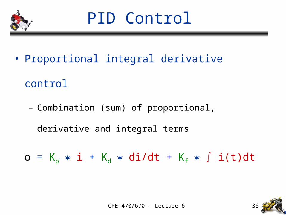
PID Control
• Proportional integral derivative control
– Combination (sum) of proportional, derivative and integral
terms
o = Kp i + Kd di/dt + Kf i(t)dt
CPE 470/670 - Lecture 6 37
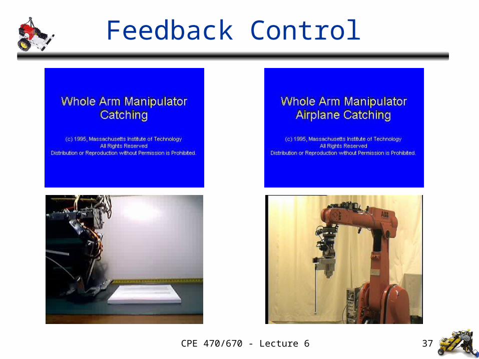
Feedback Control
CPE 470/670 - Lecture 6 38
Readings
• F. Martin: Chapter 5
• M. Matarić: Chapter 10