The Robotics InstituteCarnegie Mellon University

5000 Forbes AvenuePittsburgh, PA 15213

January 1999

©1999 Carnegie Mellon University

Autonomous Cross-Country Navigation UsingStereo Vision

Sanjiv Singh and Bruce Digney

CMU-RI-TR-99-03

This work was sponsored by the Defence Research Establishment, Suffield, Canada under contract W7702-6-R577/001 "Performance Improvements for Autonomous Cross-Country Navigation".

ii

iii

Abstract

This paper reports on an autonomous robot designed for operation in unchartedoutdoor environments. To accomplish this we have developed a robot vehicleequipped with wide field-of-view stereo vision and high accuracy inertial naviga-tion. The software resident onboard the vehicle uses binoculor cameras, mountedin a novel configuration, to produce dense range maps of the environment. Thisdata is used to guide the vehicle around obstacles and the incremental map that isdeveloped from range data taken from the moving vehicle is used to dynamicallyalter the route to the final destination. Additionally, we have investigated the pos-sibility of merging range data from scanning lasers and stereo vision in order toachieve high performance and high bandwidth.

iv

page iii

iii

Table of Contents

1. Introduction 5

2. Camera Calibration and Rectification 7

2.1 Camera Configuration: Vertical vs. Horizontal Baseline 72.2 Calibration 10

2.2.1 Method of Calibration 102.2.2 Calibration using Moravec's Method 102.2.3 Calibration of WFOV camera/lenses using Tsai's method 16

2.3 Rectification 182.3.1 Method of Rectification 192.3.2 Determination of the Rectification Matrix 192.3.3 Rectification Procedure 21

3. Stereo Range Processing 27

3.1 Performance 273.1.1 Setup 273.1.2 Number of Disparities Searched. 293.1.3 Resolution 313.1.4 Clipping 32

3.2 Summary 37

4. Local Navigation 39

4.1 Experiments with Ranger 434.1.1 Steep Wall 434.1.2 Sand Pile 44

4.2 Path tracking with Ranger 464.2.1 Waypoint Navigation 464.2.2 Repeating Closed Path 48

4.3 Summary 49

5. Global Navigation 51

5.1 Map Representation 525.1.1 Regular Grids 525.1.2 Quadtrees 535.1.3 Framed Quadtrees 53

5.2 Incremental Planning 535.3 Simulation Results 55

5.3.1 Traverse Length 565.3.2 Memory Usage 575.3.3 Execution Time 57

5.4 Test Results on Autonomous Vehicle 595.5 Summary 61

iv

6. Laser and Stereo Merging 63

6.1 Laser range finder 636.2 Comparison of Laser and Stereo range finders 636.3 Performance of Z+F Laser Scanner 646.4 Combining Laser and Stereo Range Information 656.5 Merging of range information 656.6 Summary 66

7. References 73

5

1. Introduction

While it is clear that autonomous navigation in natural terrains would be desirable it is also clear

that it is a very difficult problem. Autonomous navigation in indoor environments is almost com-

mon place, but these robots have the benefit of a priori knowledge of the environment structure

and sometimes even installed navigation aids and infrastructure. For outdoor navigation in

unstructured environments the amount of information that can be assumed is considerable less

and the placement of artificial navigation aids is impractical. Therefore autonomous outdoor nav-

igation requires considerably more information be perceived and that more complex decisions be

made using that information.

Unmanned outdoor vehicles cannot assume that the terrain is uniformly flat and that all obstacles

are discrete and that control decisions are of a binary nature (passable or not passable). For out-

door vehicles the terrain is not uniform and in addition to discrete obstacles the terrain is repre-

sented by varying degrees of passablity. That is the terrain and potential paths through that terrain

would be ranked by the amount of roll and pitch that would result. For different vehicles different

amounts of roll and pitch would be acceptable. It is the purpose of the perception system to view

the terrain that can be crossed by the vehicle and it is the purpose of the navigation control system

to make decisions about which path, when weighed with the desired destination of the vehicle, to

take.

This document reports on improvements to a basic autonomous cross country vehicle that was

developed for an earlier program [20]. The previous program developed navigation and collision

avoidance using stereo vision and precise inertial positioning. In the current program we have

investigated three major improvements:

• Wider Field of View.One deficiency noted in the previous system was that the field ofview produced by the stereo vision system was too narrow. Hence, we have developed anewer system with a wider field of view.

• Incorporation of Global Planning.While local navigation is able to generally maintain acourse towards a goal while avoiding obstacles, it cannot deal with situations in whichthe robot must backtrack or choose an action which is suboptimal in the short term butwill provide long term benefit. On-line global planning produces an altered route for anautonomous vehicle as the environment is discovered.

• Combination of Stereo Vision and Laser Ranging. To date most autonomous systemshave used a single mode (stereo vision or laser ranging) of building a three dimensional

6

description of the world. In this report we discuss experiments aimed at evaluating thecombination of these two modalities.

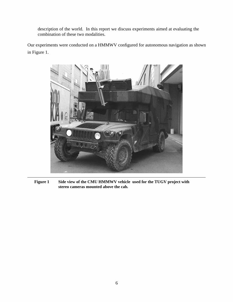
Our experiments were conducted on a HMMWV configured for autonomous navigation as shown

in Figure 1.

Figure 1 Side view of the CMU HMMWV vehicle used for the TUGV project withstereo cameras mounted above the cab.

7

2. Camera Calibration and Rectification

Autonomous vehicles operating in off-road conditions must perceive the shape of the surrounding

terrain in order to navigate safely through obstacles. Perception must be both fast and accurate. In

addition, we have found from past experience that for practical reasons of speed and scale, a sin-

gle view that the vehicle has of the world must be large. In earlier work we developed a stereo

vision system with a narrower field of view (approximately 50 degrees) that was ported to an

autonomous HMMWV (Highly Mobile Multi-Wheeled Vehicle) [20].

Although successful within the initial scope of the project, it was clear that a wider field of view

would substantially improve performance. The narrow FOV cameras that were used resulted in a

control situation that was analogous to driving with tunnel vision. Since the vehicle could only

turn onto terrain that it observed as safe (having no obstacles, dangerous slopes or drop-offs),

maneuverability of the vehicle was severely restricted and the it could not operate to its full abil-

ity. In response to these limitations we have developed a stereo system with a wide field of view.

Unfortunately, the optics required to produce the necessary field of view produce significant dis-

tortion and must be corrected before the images can used by the stereo vision processing.

This section summarizes procedures we have developed to correct the lens distortion. In addition,

we discuss a process called “rectification” that compensates for non-parallel optical axes. In some

cases this effect is due to misaligned CCD arrays, but it is also common to get some error due to

mechanical misalignment of the cameras.

2.1. Camera Configuration: Vertical vs. Horizontal Baseline

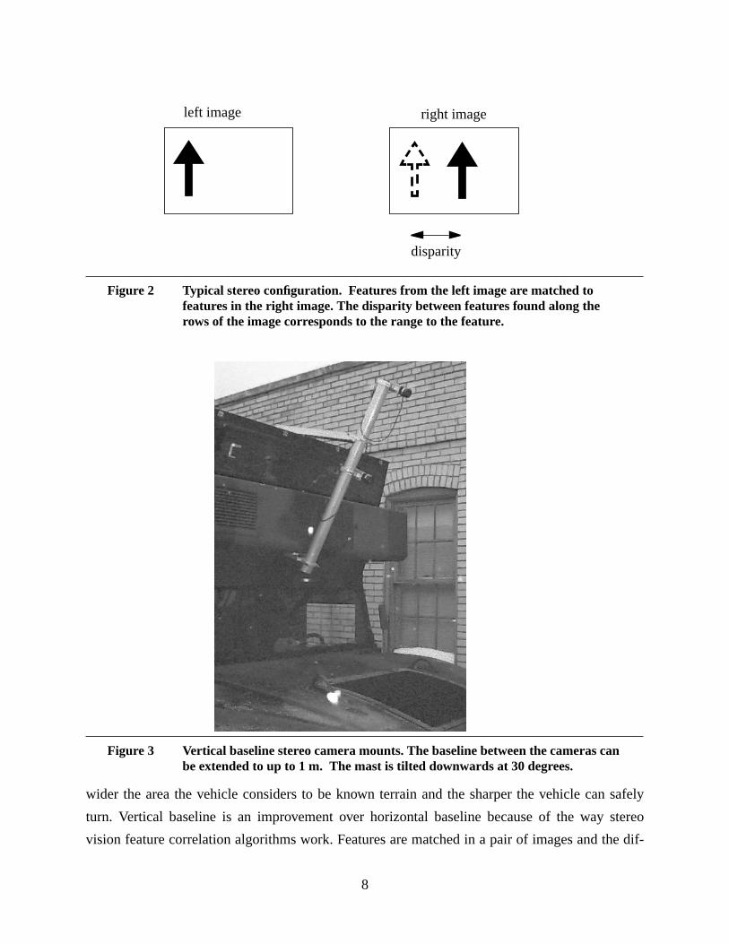
Typically, stereo vision systems use cameras that are horizontally aligned. That is, cameras are

placed at the same elevation. The process of stereo vision is then typically defined as finding a

match between features in left and right images as shown in Figure 2.

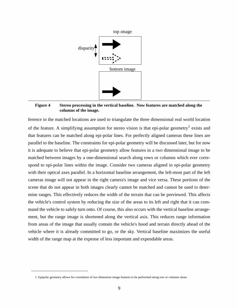
Our stereo system uses a vertical baseline (Figure 3) where the cameras are placed one on top of

the other on a mast that is tilted downwards. In this case, the process of stereo vision consists of

finding match between top and bottom images as shown in Figure 4.

The advantage of vertical baseline stereo is that it maximizes usable range information in the hor-

izontal direction to the front of the vehicle. Range information is then used to generate2 1/2 D

terrain maps from which the steering decisions are made. The wider that the terrain map is the

8

wider the area the vehicle considers to be known terrain and the sharper the vehicle can safely

turn. Vertical baseline is an improvement over horizontal baseline because of the way stereo

vision feature correlation algorithms work. Features are matched in a pair of images and the dif-

Figure 2 Typical stereo configuration. Features from the left image are matched tofeatures in the right image. The disparity between features found along therows of the image corresponds to the range to the feature.

Figure 3 Vertical baseline stereo camera mounts. The baseline between the cameras canbe extended to up to 1 m. The mast is tilted downwards at 30 degrees.

left image right image

disparity

9

ference in the matched locations are used to triangulate the three dimensional real world location

of the feature. A simplifying assumption for stereo vision is that epi-polar geometry1 exists and

that features can be matched along epi-polar lines. For perfectly aligned cameras these lines are

parallel to the baseline. The constraints for epi-polar geometry will be discussed later, but for now

it is adequate to believe that epi-polar geometry allow features in a two dimensional image to be

matched between images by a one-dimensional search along rows or columns which ever corre-

spond to epi-polar lines within the image. Consider two cameras aligned in epi-polar geometry

with their optical axes parallel. In a horizontal baseline arrangement, the left-most part of the left

cameras image will not appear in the right camera's image and vice versa. These portions of the

scene that do not appear in both images clearly cannot be matched and cannot be used to deter-

mine ranges. This effectively reduces the width of the terrain that can be previewed. This affects

the vehicle's control system by reducing the size of the areas to its left and right that it can com-

mand the vehicle to safely turn onto. Of course, this also occurs with the vertical baseline arrange-

ment, but the range image is shortened along the vertical axis. This reduces range information

from areas of the image that usually contain the vehicle's hood and terrain directly ahead of the

vehicle where it is already committed to go, or the sky. Vertical baseline maximizes the useful

width of the range map at the expense of less important and expendable areas.

Figure 4 Stereo processing in the vertical baseline. Now features are matched along thecolumns of the image.

1. Epipolar geometry allows for correlation of two dimension image features to be performed along row or columns alone.

top image

bottom image

disparity

10

2.2. Calibration

In order for stereo correlation techniques to work properly and for the range results that they yield

to be accurate and representative of the real world, the effects of the camera/lens distortion must

often be accounted for. In previous work with smaller FOV camera/lenses the distortion effects

were found to be negligible, but with the WFOV used in this study the effects were significant and

would have to be considered.

The process of camera calibration is generally performed by first assuming a simplified model for

both the camera and the distortion of resulting images and then statistically, usually using a Least

Mean Squares (LMS) technique, fitting the distortion model to the observed distortion. Once the

distortion has been modeled, it can be applied to the distorted image to correct it. An idealized pin

hole camera model and radially symmetric lenses distortion are the usual modeling assumptions.

Many calibration techniques also take into account distortion created by the digitization effects of

CCD cameras. These effects are modeled along with the optical distortion and together account

for the overall distortion observed in the acquired digital image.

Once a model of the camera and distortion have been chosen they are fit to the real camera/lens by

comparing where points of accurately know real world coordinates appear in the image and where

they would appear if there was no distortion. The error is minimized over as many points as is rea-

sonable to fit distortion correction function to the distortion observed in the test scene. This distor-

tion correction function, when applied to a raw image, reduces the distortion and what appears as

a straight line in the real world appears as a straight line in the image.

2.2.1. Method of Calibration

Two calibration techniques were tried: A method developed by Tsai [1] and a second method

developed by Moravec [2]. The major difference was that the implementation Tsai's method

assumed that the center of the radially symmetric distortion is the center of the image, while

Moravec's method performs an initial search for the center of the distortion. Given the high degree

of distortion and the that the distortion was not centered within the image resulting from the

WFOV cameras used, Moravec's method gave much better results.

2.2.2. Calibration using Moravec's Method

To calibrate the camera/lenses, a single image of a target scene is captured. The target scene is an

accurately laid out rectangular grid of three inch diameter dark colored spots with three inch spac-

11

ing between them on a white board. The camera is aligned normal to the image plane and adjusted

to get as much of the spot grid within its field of view as possible. The camera is aimed at the cen-

ter of the grid which is roughly marked with an extra spot. Once that the image is captured, the

extra spot will be used by the spot matching/spot locating algorithm as the center of reference of

the grid. When the center spot of the spot grid has been determined, each additional detected spot

can be identified relative to the center spot and accurately known spatial coordinates can be used

to generate an ideal image location (pin-hole camera model) of the spot to be compared with the

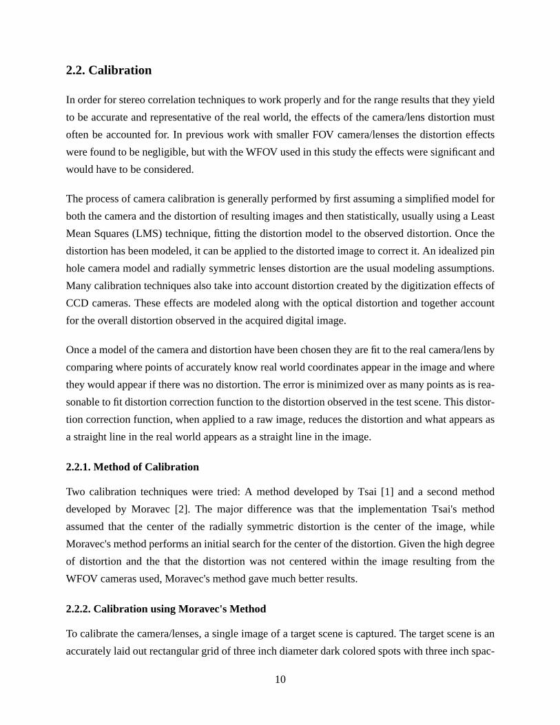
actual spot position (affected by distortion) in the image. Shown in Figure 5 is the distorted image

of the regularly spaced rectangular grid of spots obtained through the 110 degree FOV camera/

lens.

Notice the severe bowing of what should be straight lines of spots in a rectangular grid. Although

it is difficult to detect careful examination shows that the distortion is not centered in the image.

The first step of the calibration procedure (implemented in the programflatfish.c ) is to auto-

matically detect the spots and spot locations from the raw image. This is done with a template

matching technique using circular shaped templates. These circular templates worked very well

for less distorted images and in the center of more severely distorted images, but missed many

Figure 5 Raw image of a regular rectangular grid of three inch diameter spots.

12

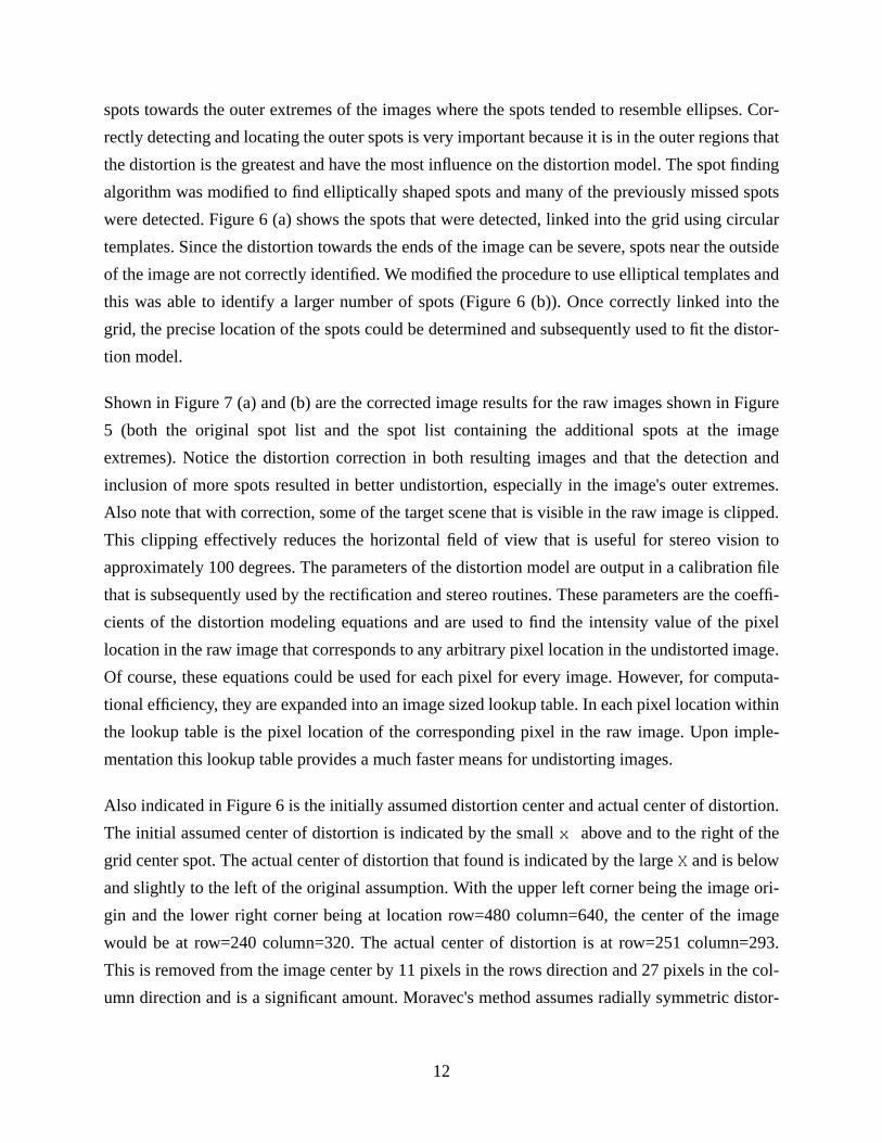
spots towards the outer extremes of the images where the spots tended to resemble ellipses. Cor-

rectly detecting and locating the outer spots is very important because it is in the outer regions that

the distortion is the greatest and have the most influence on the distortion model. The spot finding

algorithm was modified to find elliptically shaped spots and many of the previously missed spots

were detected. Figure 6 (a) shows the spots that were detected, linked into the grid using circular

templates. Since the distortion towards the ends of the image can be severe, spots near the outside

of the image are not correctly identified. We modified the procedure to use elliptical templates and

this was able to identify a larger number of spots (Figure 6 (b)). Once correctly linked into the

grid, the precise location of the spots could be determined and subsequently used to fit the distor-

tion model.

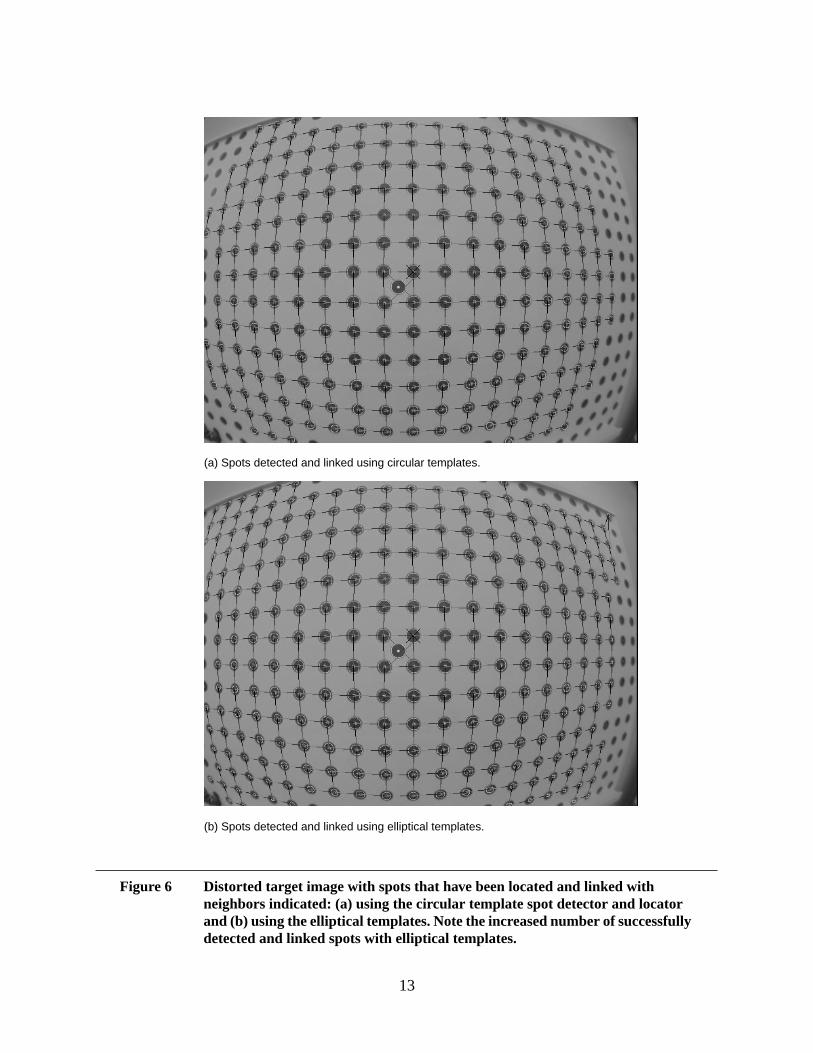
Shown in Figure 7 (a) and (b) are the corrected image results for the raw images shown in Figure

5 (both the original spot list and the spot list containing the additional spots at the image

extremes). Notice the distortion correction in both resulting images and that the detection and

inclusion of more spots resulted in better undistortion, especially in the image's outer extremes.

Also note that with correction, some of the target scene that is visible in the raw image is clipped.

This clipping effectively reduces the horizontal field of view that is useful for stereo vision to

approximately 100 degrees. The parameters of the distortion model are output in a calibration file

that is subsequently used by the rectification and stereo routines. These parameters are the coeffi-

cients of the distortion modeling equations and are used to find the intensity value of the pixel

location in the raw image that corresponds to any arbitrary pixel location in the undistorted image.

Of course, these equations could be used for each pixel for every image. However, for computa-

tional efficiency, they are expanded into an image sized lookup table. In each pixel location within

the lookup table is the pixel location of the corresponding pixel in the raw image. Upon imple-

mentation this lookup table provides a much faster means for undistorting images.

Also indicated in Figure 6 is the initially assumed distortion center and actual center of distortion.

The initial assumed center of distortion is indicated by the smallx above and to the right of the

grid center spot. The actual center of distortion that found is indicated by the largeX and is below

and slightly to the left of the original assumption. With the upper left corner being the image ori-

gin and the lower right corner being at location row=480 column=640, the center of the image

would be at row=240 column=320. The actual center of distortion is at row=251 column=293.

This is removed from the image center by 11 pixels in the rows direction and 27 pixels in the col-

umn direction and is a significant amount. Moravec's method assumes radially symmetric distor-

13

Figure 6 Distorted target image with spots that have been located and linked withneighbors indicated: (a) using the circular template spot detector and locatorand (b) using the elliptical templates. Note the increased number of successfullydetected and linked spots with elliptical templates.

(a) Spots detected and linked using circular templates.

(b) Spots detected and linked using elliptical templates.

14

Figure 7 Corrected target image: (a) using the calibration points provided by thecircular template spot detector and locator and (b) including the additionalcalibration points provided from the elliptical templates.

(a) Corrected image using circular templates.

(a)

(b)

15

tion and that the distortion can be modeled by an order polynomial. The center of

distortion is located by searching the center area of the image and determining which location

yields the most consistent radially symmetric distortion. Once the center of distortion is found, the

polynomial (whose order is specified by the user) relating the distorted radius, , to the cor-

rected radius, :

is fit to the image and spot data.

One can think of the process of distortion correction as an operation of finding the corresponding

pixel in the raw image for each pixel in the corrected image. This is done by first finding the radial

distance away from the center of distortion for the corrected image pixel location in question. The

radius in the corrected image can then be stretched using the distortion function to find the corre-

sponding distorted radius length. This radial length can then be used to find the pixel location in

the raw image that corresponds to the pixel location in the corrected image. Once this is known,

the pixel value (or intensity) in the corrected image is set to the value of its corresponding pixel in

the raw image.

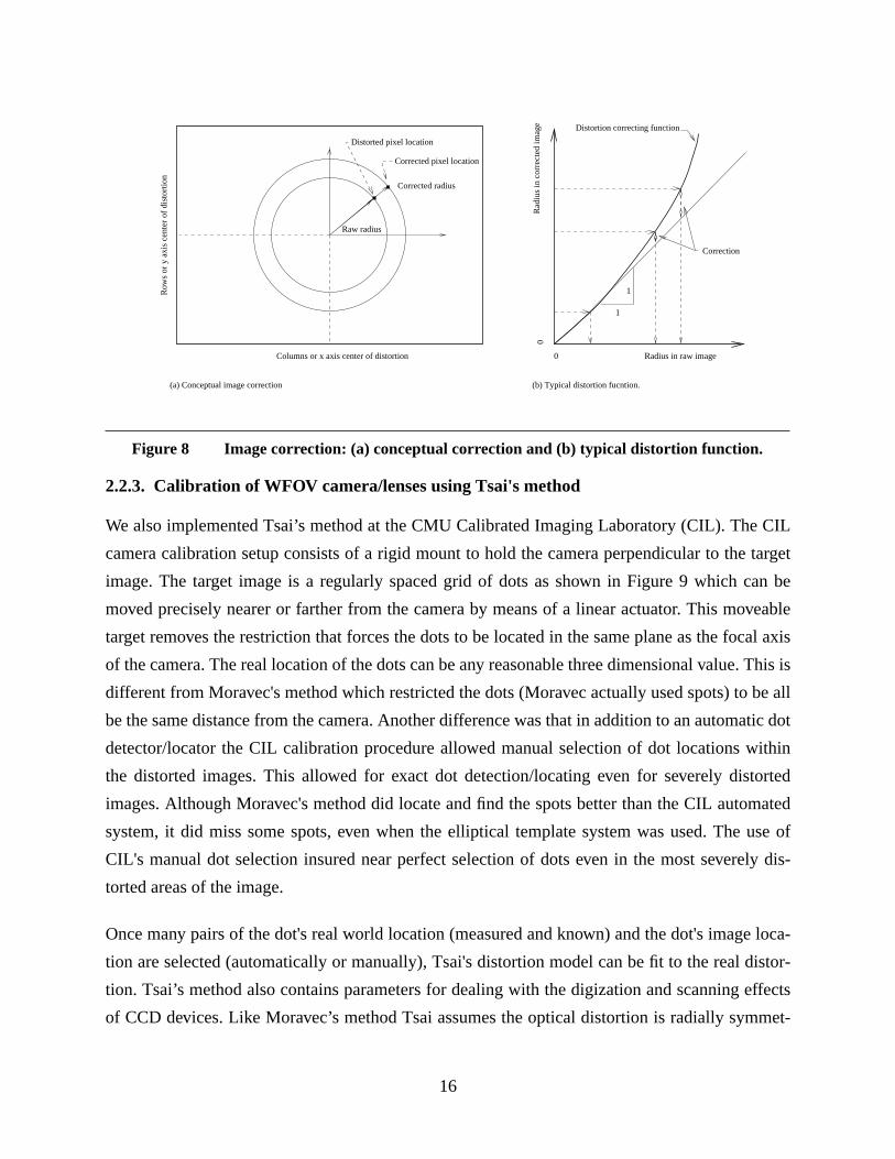
Figure 8(a) conceptually shows this radial correction process and Figure 8 (b) shows a typical dis-

tortion correction function. Note in Figure 8 (b) the increasing distortion towards away from the

distortion center and towards the edge of the image. For comparison a unity slope line is added.

This line represents what the distortion correction function would be if there was no distortion.

From this it can be concluded that in order to correct the imaged the raw image must be stretched

an ever increasing amount the farther one gets from the distortion center. This results in the clip-

ping of some of the target scene in the corrected image. This makes sense because all of the target

scene fits in the raw image only because of the compressive effects of the distortion. Clipping

results in a reduction of field of view useful for stereo vision that is nonlinear with distance from

the center. That is, the degree to which the horizontal field of view is clipped is greater than that of

the vertical field of view because the field of view is wider than it is high and hence the horizontal

axis is affected more.

(1)

nth

rdis

r cor

rdis ko k1r cor k2r2cor … knr

ncor+ + + +=

16

2.2.3. Calibration of WFOV camera/lenses using Tsai's method

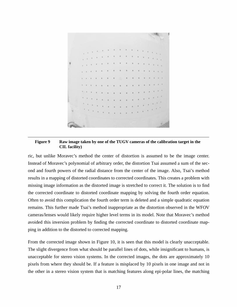
We also implemented Tsai’s method at the CMU Calibrated Imaging Laboratory (CIL). The CIL

camera calibration setup consists of a rigid mount to hold the camera perpendicular to the target

image. The target image is a regularly spaced grid of dots as shown in Figure 9 which can be

moved precisely nearer or farther from the camera by means of a linear actuator. This moveable

target removes the restriction that forces the dots to be located in the same plane as the focal axis

of the camera. The real location of the dots can be any reasonable three dimensional value. This is

different from Moravec's method which restricted the dots (Moravec actually used spots) to be all

be the same distance from the camera. Another difference was that in addition to an automatic dot

detector/locator the CIL calibration procedure allowed manual selection of dot locations within

the distorted images. This allowed for exact dot detection/locating even for severely distorted

images. Although Moravec's method did locate and find the spots better than the CIL automated

system, it did miss some spots, even when the elliptical template system was used. The use of

CIL's manual dot selection insured near perfect selection of dots even in the most severely dis-

torted areas of the image.

Once many pairs of the dot's real world location (measured and known) and the dot's image loca-

tion are selected (automatically or manually), Tsai's distortion model can be fit to the real distor-

tion. Tsai’s method also contains parameters for dealing with the digization and scanning effects

of CCD devices. Like Moravec’s method Tsai assumes the optical distortion is radially symmet-

Figure 8 Image correction: (a) conceptual correction and (b) typical distortion function.

(b) Typical distortion fucntion.

Distorted pixel location

Corrected pixel locationR

ows

or y

axi

s ce

nter

of

dist

ortio

n

Columns or x axis center of distortion

Raw radius

Rad

ius

in c

orre

cted

imag

e

Radius in raw image

1

1

Correction

0

0

Corrected radius

(a) Conceptual image correction

Distortion correcting function

17

ric, but unlike Moravec’s method the center of distortion is assumed to be the image center.

Instead of Moravec’s polynomial of arbitrary order, the distortion Tsai assumed a sum of the sec-

ond and fourth powers of the radial distance from the center of the image. Also, Tsai’s method

results in a mapping of distorted coordinates to corrected coordinates. This creates a problem with

missing image information as the distorted image is stretched to correct it. The solution is to find

the corrected coordinate to distorted coordinate mapping by solving the fourth order equation.

Often to avoid this complication the fourth order term is deleted and a simple quadratic equation

remains. This further made Tsai’s method inappropriate as the distortion observed in the WFOV

cameras/lenses would likely require higher level terms in its model. Note that Moravec’s method

avoided this inversion problem by finding the corrected coordinate to distorted coordinate map-

ping in addition to the distorted to corrected mapping.

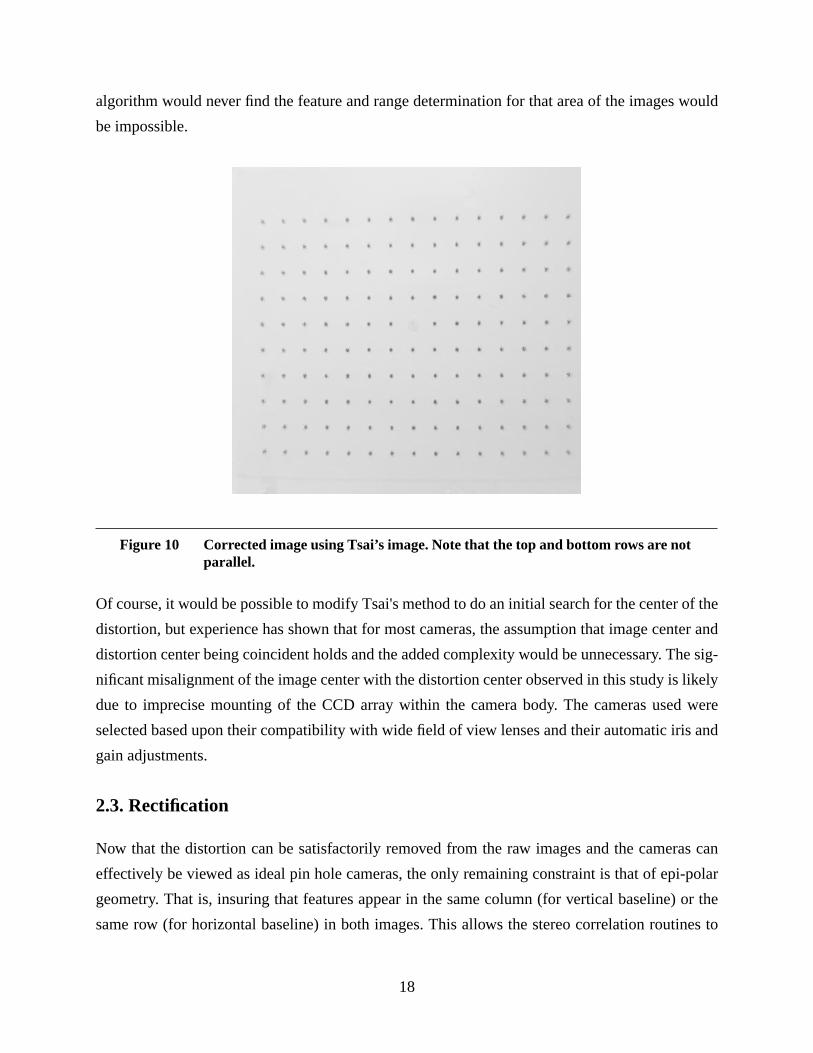
From the corrected image shown in Figure 10, it is seen that this model is clearly unacceptable.

The slight divergence from what should be parallel lines of dots, while insignificant to humans, is

unacceptable for stereo vision systems. In the corrected images, the dots are approximately 10

pixels from where they should be. If a feature is misplaced by 10 pixels in one image and not in

the other in a stereo vision system that is matching features along epi-polar lines, the matching

Figure 9 Raw image taken by one of the TUGV cameras of the calibration target in theCIL facility)

18

algorithm would never find the feature and range determination for that area of the images would

be impossible.

Of course, it would be possible to modify Tsai's method to do an initial search for the center of the

distortion, but experience has shown that for most cameras, the assumption that image center and

distortion center being coincident holds and the added complexity would be unnecessary. The sig-

nificant misalignment of the image center with the distortion center observed in this study is likely

due to imprecise mounting of the CCD array within the camera body. The cameras used were

selected based upon their compatibility with wide field of view lenses and their automatic iris and

gain adjustments.

2.3. Rectification

Now that the distortion can be satisfactorily removed from the raw images and the cameras can

effectively be viewed as ideal pin hole cameras, the only remaining constraint is that of epi-polar

geometry. That is, insuring that features appear in the same column (for vertical baseline) or the

same row (for horizontal baseline) in both images. This allows the stereo correlation routines to

Figure 10 Corrected image using Tsai’s image. Note that the top and bottom rows are notparallel.

19

search in one-dimension rather than two. In this study a vertical baseline was chosen to give the

widest possible terrain map in front of the vehicle. With vertical baseline one camera is mounted

above the other and the stereo correlation is performed between the corresponding columns of the

two images. It is impossible to insure sufficiently precise mechanical alignment of the cameras so

a software alignment is used. Effectively, a transition matrix is determined and applied to one

image to bring it into epi-polar alignment with the other. This process is called rectification and

should be performed whenever the cameras are mounted or whenever the camera alignment is

otherwise suspect.

2.3.1. Method of Rectification

Rectification is performed by hand selecting matching features in a pair of images. Two types of

features are selected; First are the features that are effectively at infinite range (disparity is less

than one pixel width) and should have zero disparity. These features should occupy the same loca-

tion, both column and row coordinates, in both images. Selected second are the features that

should have a non-zero disparity and are within the working range of the stereo correlation algo-

rithms. For vertical baseline stereo these features should be in the same column, but different row,

and for horizontal baseline they should be in the same row but different column. Once some num-

ber of features have been selected (the more the better), an LMS fit yields the transformation

matrix that will translate and rotate one image to bring it into epi-polar geometry with the other.

Note that the rectification program produces two matrices, one for each image. However, one is

simply an identity matrix, while the other does the meaningful transformation. Again, in the pur-

suit of computational efficiency, the rectification transformations are represented by two image

sized lookup tables.

2.3.2. Determination of the Rectification Matrix

The aim of stereo rectification is to warp the second (bottom) image, so that the pair satisfies the

epi-polar geometry and infinity range constraints.

Image rectification can be done by using;

(2)c'

r '

1

H3 3×

c

r

1

=

20

where is the original image coordinate and is the rectified image coordinate. The

objective is to find which warps the second image to suit the epipolar geometry and the

infinity range constraints.

This can be done by hand picking a number of matching features in the two images to find a leastsquare solution.

1. To find , pick i-matching features from the top & bottom image. We use columns (c1i) fromthe top image and the associated columns & rows (c2i, r2i) from the bottom image to solve for

;

(3)

Which takes the form of;

(4)

To solve for using Pseudo-Inverse;

(5)

Which actually looks like;

(6)

2. Using the same method, can be solved using rows (r1i) from the top image andthe associated columns & rows (c2i, r2i) from the bottom image that have matching features atinfinite range. The equation is;

(7)

3. With H00, H01, H02, H10, H11, andH12, the rectification matrix is solved;

c r 1T

c' r ' 1T

H3 3×

H0 j

H00 H01 H02, ,

c10

c11

…c1i

c20 r20 1

c21 r21 1

… … …c2i r2i 1

H00

H01

H02

=

y Ax=

x

x AT

A( )1–A

T( )y=

H00

H01

H02

c20 r20 1

c21 r21 1

… … …c2i r2i 1

Tc20 r20 1

c21 r21 1

… … …c2i r2i 1

1–

c20 r20 1

c21 r21 1

… … …c2i r2i 1

T

=

c10

c11

…c1i

H10 H11 H12, ,

H10

H11

H12

c20 r20 1

c21 r21 1

… … …c2i r2i 1

Tc20 r20 1

c21 r21 1

… … …c2i r2i 1

1–

c20 r20 1

c21 r21 1

… … …c2i r2i 1

T

=

r10

r11

…r1i

21

(8)

2.3.3. Rectification Procedure

A scene in which some of the image contains features at infinity and many clear features within

the expected working range of the stereo algorithm is required. Rectification is performed by the

programeasyrect . This program takes the two raw images, the camera calibration parameter

files and outputs the rectificationH matrices. Upon runningeasyrect , two undistorted images

for the left and right (or top and bottom) cameras are displayed. By following the instructions that

are also displayed, features can be selected alternately in one image and then in the other image.

Features that should share both coordinates are selected by positioning the pointer of the mouse

over the feature and hitting “b” for both. Likewise, for features that should share the column coor-

dinate by hitting “c” for column and for features that should share the row coordinate by hitting

“r” for row. Also, by depressing the appropriate mouse button the windows will zoom in and out

allowing precise selection of the exact pixel that best represents a particular feature.

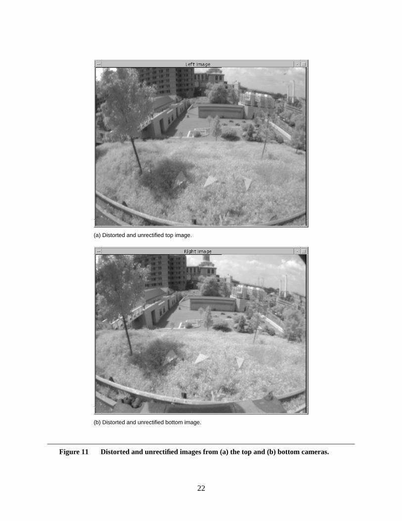
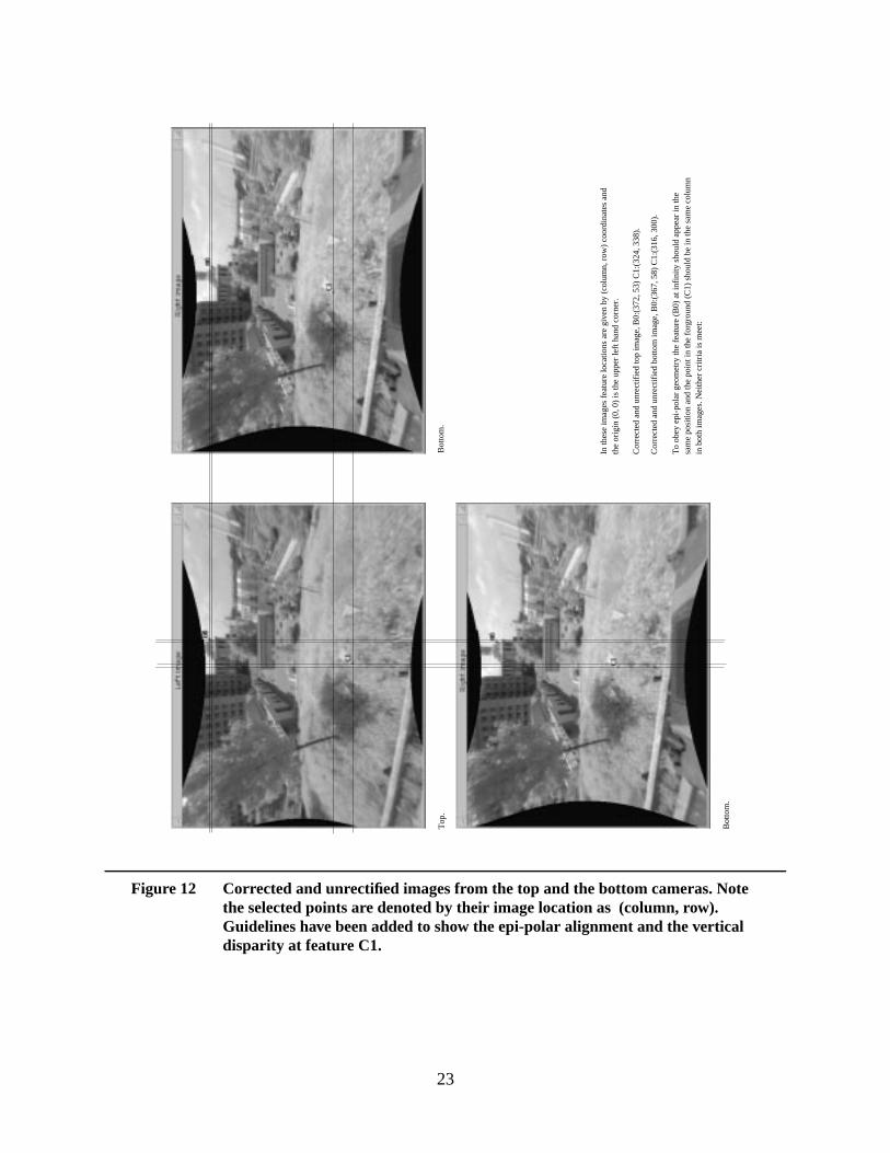
The raw images for the top and bottom cameras are shown in Figure 11. Notice that the effects of

distortion are seen as bowing of what should be straight lines. Figure 12 shows the unrectified (but

corrected) images of a test scene. Note that neither of the epi-polar constraints are met.

Disparity at infinity is not zero. From these images it is seen that the featureB0 selected on the

tower (for our purposes at infinity) does not occupy the same location in the top and bottom

images. Its top location is column 372 and row 53, while in the bottom image its location is col-

umn 367 and row 58, a difference of 5 pixels in each axis. It is also seen that the featureC1,

selected in the foreground, is not located in the same column (remember this is vertical baseline

stereo). Its top location is column 324 and row 338, while in the bottom image its location is col-

umn 316 and row 300, a difference of 8 pixels along the column axis. In this case, the difference

along the row axis would be the disparity and will eventually be used to determine the range.

After further selection of features and application of the resulting transformation matrices, the

images are aligned to epi-polar geometry as shown in Figure 13. The featureB0 at infinity is

aligned within 1 pixel width along each axis and the featureC1 is aligned within 1 pixel along the

column axis. The difference in location along the row axis is 338-305=33 pixels, which is the dis-

parity for the feature.

H3 3×

H00 H01 H02

H10 H11 H12

0 0 1

=

22

Figure 11 Distorted and unrectified images from (a) the top and (b) bottom cameras.

(a) Distorted and unrectified top image.

(b) Distorted and unrectified bottom image.

23

Figure 12 Corrected and unrectified images from the top and the bottom cameras. Notethe selected points are denoted by their image location as (column, row).Guidelines have been added to show the epi-polar alignment and the verticaldisparity at feature C1.

Bot

tom

.

Top

.B

otto

m.

In th

ese

imag

es f

eatu

re lo

catio

ns a

re g

iven

by

(col

umn,

row

) co

ordi

nate

s an

dth

e or

igin

(0,

0)

is th

e up

per

left

han

d co

rner

.

To

obey

epi

-pol

ar g

eom

etry

the

feat

ure

(B0)

at i

nfin

ity s

houl

d ap

pear

in th

esa

me

posi

tion

and

the

poin

t in

the

forg

roun

d (C

1) s

houl

d be

in th

e sa

me

colu

mn

in b

oth

imag

es. N

eith

er c

ritr

ia is

mee

t:

Cor

rect

ed a

nd u

nrec

tifie

d to

p im

age,

B0:

(372

, 53)

C1:

(324

, 338

).

Cor

rect

ed a

nd u

nrec

tifie

d bo

ttom

imag

e, B

0:(3

67, 5

8) C

1:(3

16, 3

00).

24

Figure 13 Corrected and rectified images from the top and the bottom cameras. Note theselected points are denoted by their image location as (column, row).Guidelines have been added to show the epi-polar miss-alignment.

The

top

and

botto

m im

ages

now

obe

y th

e ep

i-po

lar

cons

trai

nts.

The

dif

fere

nce

in th

e ve

rica

l pos

ition

of

C1

is th

e di

spar

ity a

ndis

use

d to

det

erm

ine

the

rang

e of

that

fea

ture

.

Bot

tom

.

Top

.B

otto

m.

In th

ese

imag

es f

eatu

re lo

catio

ns a

re g

iven

by

(col

umn,

row

) co

ordi

nate

s an

dth

e or

igin

(0,

0)

is th

e up

per

left

han

d co

rner

.

Cor

rect

ed a

nd r

ectif

ied

top

imag

e, B

0:(3

73, 5

3) C

1:(3

25, 3

38).

Cor

rect

ed a

nd r

ectif

ied

botto

m im

age,

B0:

(374

, 54)

C1:

(326

, 305

).

25

2.4. Summary

We have implemented methods of compensating for lens distortion from short focal length lenses

and the misalignment of optical axes. These methods are now a part of our stereo vision system

and are regularly in use. We have tested the corrected images with stereo vision programs as a

means of verification. The complete stereo system currently is used regularly in navigation exper-

iments with our HMMWV vehicles.

26

27

3. Stereo Range Processing

As discussed previously a vertical baseline stereo (VERBS) system has many advantages over

horizontal baseline system for vehicle navigation. The VERBS system developed for the TUGV

project utilized two cameras with a 110 degree horizontal field of view mounted with a 0.5 meter

baseline and pitched downward at 30 degrees. Stereo processing was performed on a dedicated

200MHz dual pentium pro processor and the resulting disparity (from which range is determined)

were sent via inter process communications to navigation modules running on a SPARC 20 pro-

cessor. In this section typical results from the VERBS system will be presented and various trade-

offs between the quality of the information and the speed of the processing will be discussed.

3.1 Performance

The VERBS vision system has many internal parameters that can be adjusted to make it better

suited to some applications and usually less suited to others. In this section some of these trade-

offs will be discussed and quantified. For the control and navigation of moving vehicles, the rate

at which the new range information is available and the quality if that information are both impor-

tant. These two criteria are pitted against each other and some compromise between quality of

data and speed must be reached. In the following subsections parameters that effect the speed and

quality of the range information produced by the TUGV’s VERBS system will be investigated.

3.1.1 Setup

To test some of the speed vs. quality trade-offs the stereo vision system was set viewing a scene

was of an area that is used to stockpile rubble. The terrain around the stock pile was basically flat

with some minor ruts and potholes. Dump trucks would backup to the face of the pile and dump

loads of bricks, soil and various debris leaving naturally slumped mounds of rubble against the

face of the stockpile. The test scene chosen was of the face of the stockpile with two distinct

mounds within the field of view of the cameras. The TUGV was parked facing the mounds, stereo

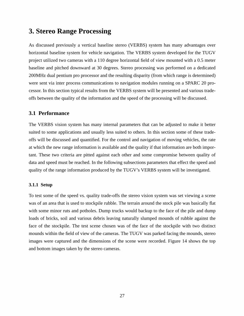
images were captured and the dimensions of the scene were recorded. Figure 14 shows the top

and bottom images taken by the stereo cameras.

28

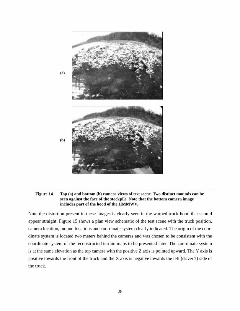
Note the distortion present in these images is clearly seen in the warped truck hood that should

appear straight. Figure 15 shows a plan view schematic of the test scene with the truck position,

camera location, mound locations and coordinate system clearly indicated. The origin of the coor-

dinate system is located two meters behind the cameras and was chosen to be consistent with the

coordinate system of the reconstructed terrain maps to be presented later. The coordinate system

is at the same elevation as the top camera with the positive Z axis is pointed upward. The Y axis is

positive towards the front of the truck and the X axis is negative towards the left (driver’s) side of

the truck.

Figure 14 Top (a) and bottom (b) camera views of test scene. Two distinct mounds can beseen against the face of the stockpile. Note that the bottom camera imageincludes part of the hood of the HMMWV.

(a)

(b)

29

3.1.2 Number of Disparities Searched.

It is unreasonable to search all locations in the image for some particular feature. In addition to

the epi-polar geometry, that reduces the search to a single column within the image, it can also be

assumed that a correct match for the current feature of interest in one image is going to be close to

the location where it appears in the other image(s). Alternately, if we have bounds on the distances

to the features we can limit out search to a smaller set of disparity values. This means testing only

a limited number disparities in the search. The choice of which disparities are used in the search

will depend upon the particular geometry of the camera setup and the expected terrain profiles.

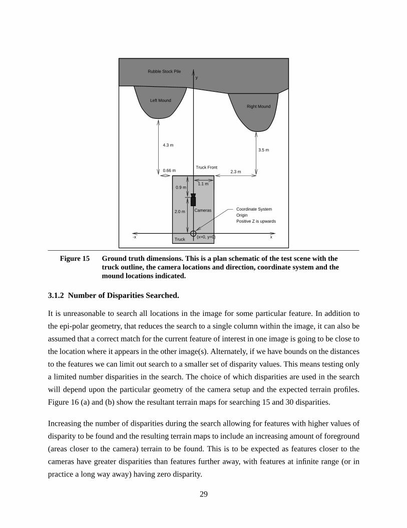
Figure 16 (a) and (b) show the resultant terrain maps for searching 15 and 30 disparities.

Increasing the number of disparities during the search allowing for features with higher values of

disparity to be found and the resulting terrain maps to include an increasing amount of foreground

(areas closer to the camera) terrain to be found. This is to be expected as features closer to the

cameras have greater disparities than features further away, with features at infinite range (or in

practice a long way away) having zero disparity.

Figure 15 Ground truth dimensions. This is a plan schematic of the test scene with thetruck outline, the camera locations and direction, coordinate system and themound locations indicated.

4.3 m

0.66 m 2.3 m

3.5 m

(x=0, y=0)-x x

1.1 m

Rubble Stock Piley

Left MoundRight Mound

Cameras

0.9 m

2.0 m

Truck

Coordinate SystemOrigin Positive Z is upwards

Truck Front

30

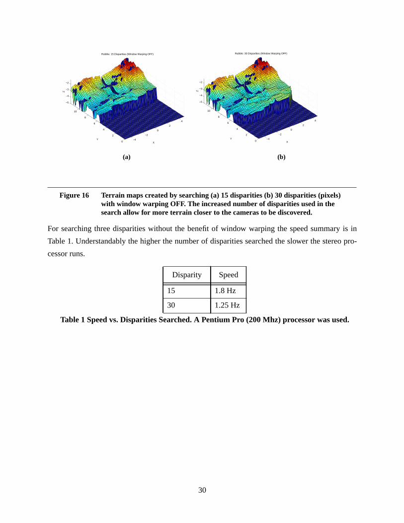
For searching three disparities without the benefit of window warping the speed summary is in

Table 1. Understandably the higher the number of disparities searched the slower the stereo pro-

cessor runs.

Figure 16 Terrain maps created by searching (a) 15 disparities (b) 30 disparities (pixels)with window warping OFF. The increased number of disparities used in thesearch allow for more terrain closer to the cameras to be discovered.

Disparity Speed

15 1.8 Hz

30 1.25 Hz

Table 1 Speed vs. Disparities Searched. A Pentium Pro (200 Mhz) processor was used.

(a) (b)

−4

−2

0

2

4

0

2

4

6

8

10

−5

−4

−3

−2

X

Rubble: 15 Disparities (Window Warping OFF)

Y

Z

−4

−2

0

2

4

0

2

4

6

8

10

−5

−4

−3

−2

X

Rubble: 30 Disparities (Window Warping OFF)

Y

Z

31

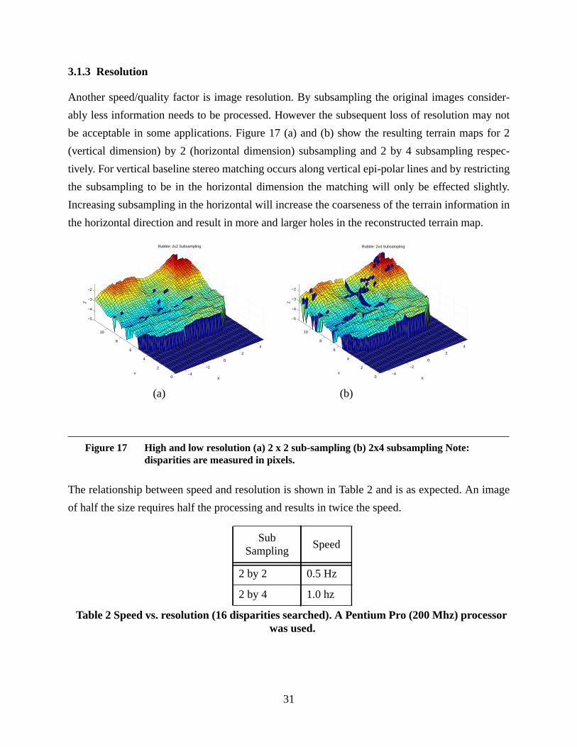
3.1.3 Resolution

Another speed/quality factor is image resolution. By subsampling the original images consider-

ably less information needs to be processed. However the subsequent loss of resolution may not

be acceptable in some applications. Figure 17 (a) and (b) show the resulting terrain maps for 2

(vertical dimension) by 2 (horizontal dimension) subsampling and 2 by 4 subsampling respec-

tively. For vertical baseline stereo matching occurs along vertical epi-polar lines and by restricting

the subsampling to be in the horizontal dimension the matching will only be effected slightly.

Increasing subsampling in the horizontal will increase the coarseness of the terrain information in

the horizontal direction and result in more and larger holes in the reconstructed terrain map.

The relationship between speed and resolution is shown in Table 2 and is as expected. An image

of half the size requires half the processing and results in twice the speed.

Figure 17 High and low resolution (a) 2 x 2 sub-sampling (b) 2x4 subsampling Note:disparities are measured in pixels.

SubSampling

Speed

2 by 2 0.5 Hz

2 by 4 1.0 hz

Table 2 Speed vs. resolution (16 disparities searched). A Pentium Pro (200 Mhz) processorwas used.

−4

−2

0

2

4

0

2

4

6

8

10

−5

−4

−3

−2

X

Rubble: 2x2 Subsampling

Y

Z

−4

−2

0

2

4

0

2

4

6

8

10

−5

−4

−3

−2

X

Rubble: 2x4 Subsampling

Y

Z

(a) (b)

32

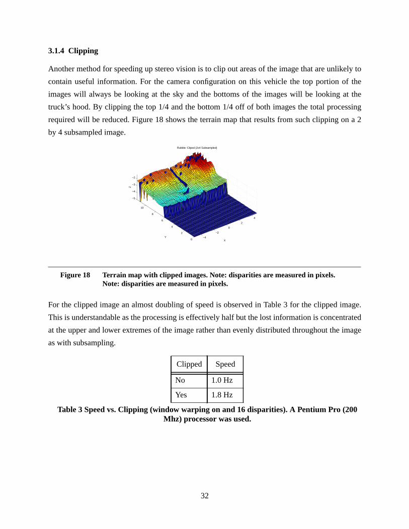
3.1.4 Clipping

Another method for speeding up stereo vision is to clip out areas of the image that are unlikely to

contain useful information. For the camera configuration on this vehicle the top portion of the

images will always be looking at the sky and the bottoms of the images will be looking at the

truck’s hood. By clipping the top 1/4 and the bottom 1/4 off of both images the total processing

required will be reduced. Figure 18 shows the terrain map that results from such clipping on a 2

by 4 subsampled image.

For the clipped image an almost doubling of speed is observed in Table 3 for the clipped image.

This is understandable as the processing is effectively half but the lost information is concentrated

at the upper and lower extremes of the image rather than evenly distributed throughout the image

as with subsampling.

Figure 18 Terrain map with clipped images. Note: disparities are measured in pixels.Note: disparities are measured in pixels.

Clipped Speed

No 1.0 Hz

Yes 1.8 Hz

Table 3 Speed vs. Clipping (window warping on and 16 disparities). A Pentium Pro (200Mhz) processor was used.

−4

−2

0

2

4

0

2

4

6

8

10

−5

−4

−3

−2

X

Rubble: Cliped (2x4 Subsampled)

Y

Z

33

3.1.5. Evaluation of Data

The ground truth for the stereo vision system was tested in two ways. Firstly a real world scene

with distances to distinguishable features at known locations was used. The known locations of

features were compared with those observed in the terrain maps. Secondly a terrain mock-up was

constructed. This terrain was approximately 5 meters by 8 meters and had a known elevation on a

0.66 meter grid. When viewed with the stereo vision system the resulting terrain map could be

compared with the known elevations at each point in the grid.

Rubble Pile. The naturally occurring scene of two mounds of rubble that were dumped on flat

ground was used to test the accuracy of the stereo system. The X and Y locations of the two

mound extremities could easily be recognized in the reconstructed terrain map were compared

with those measurements from the real terrain. From Figure 15 the locations of the tip if the right

mound are X= 3.4m and Y= 6.4m and the locations of the left mound are X = -1.7m and Y =

7.2m. These dimensions are in meters and are in the same coordinate system as the schematic of

Figure 15. The scene was viewed with the stereo vision system was set to the configuration of

window warping ON and using 16 disparities in its search. From the terrain map of Figure 16(a)

the stereo vision system yields a left mound location of X = -2.0 m and Y =7.5m and a right

mound position of X = 3.5m and Y = 7.0m. Although it is difficult to accurately resolve the loca-

tion of mounds it still can be concluded that the piles appear where they should and that the ranges

returned by stereo are accurate to about 0.3m when observing terrain in the order of 6 meters

away. Of course, just as with human vision, the accuracy of a stereo vision system improves as the

distance over which it is operating is reduced.

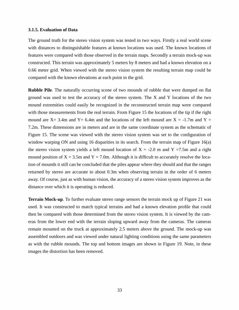
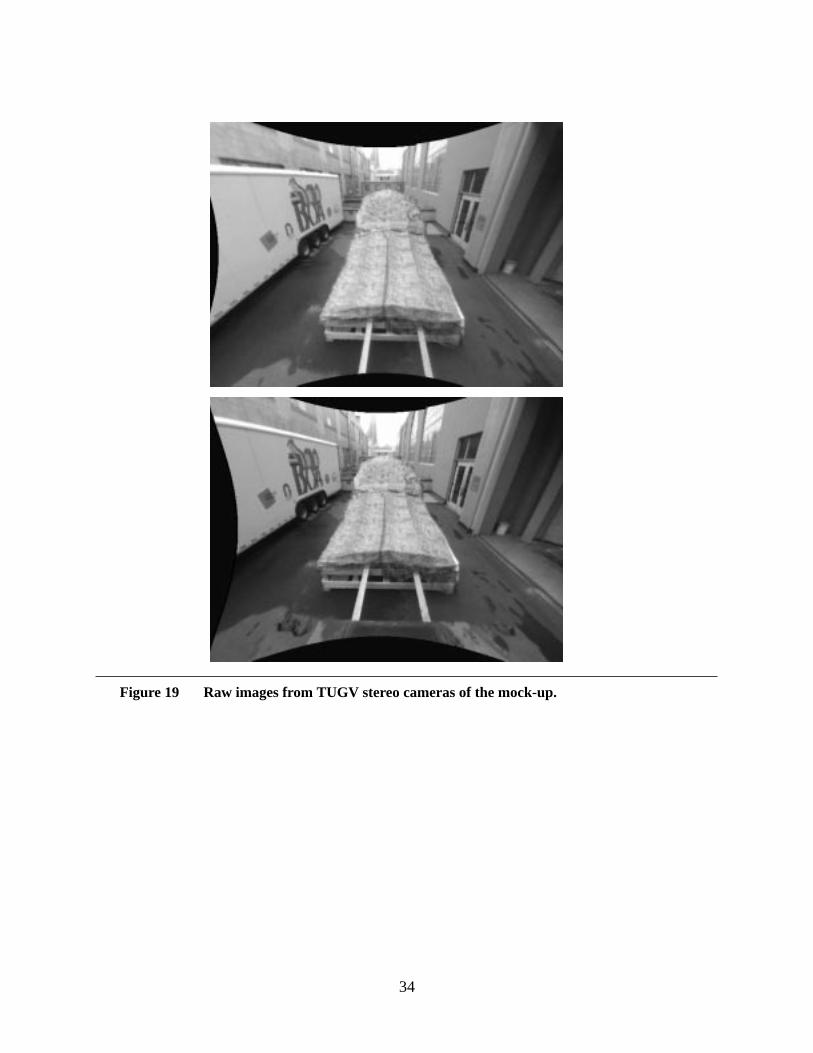
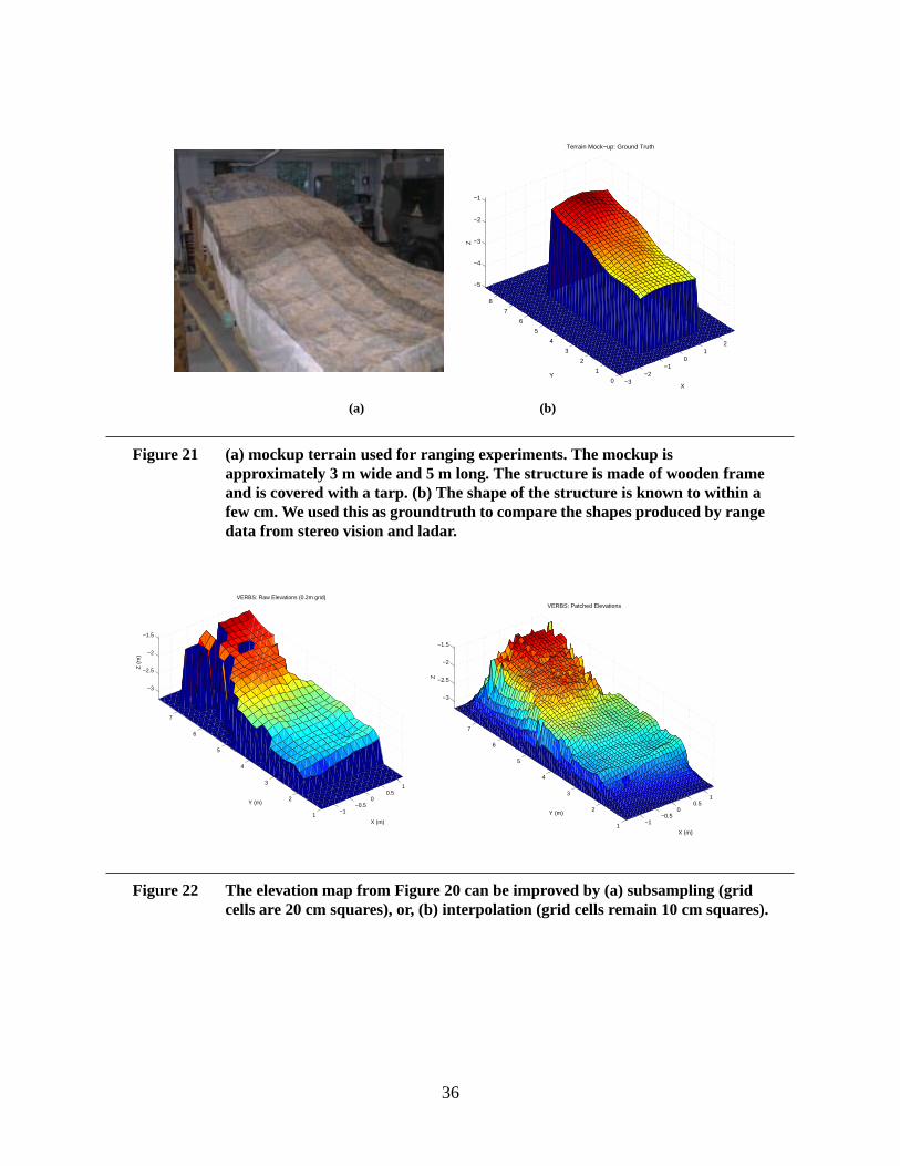
Terrain Mock-up . To further evaluate stereo range sensors the terrain mock up of Figure 21 was

used. It was constructed to match typical terrains and had a known elevation profile that could

then be compared with those determined from the stereo vision system. It is viewed by the cam-

eras from the lower end with the terrain sloping upward away from the cameras. The cameras

remain mounted on the truck at approximately 2.5 meters above the ground. The mock-up was

assembled outdoors and was viewed under natural lighting conditions using the same parameters

as with the rubble mounds. The top and bottom images are shown in Figure 19. Note, in these

images the distortion has been removed.

34

Figure 19 Raw images from TUGV stereo cameras of the mock-up.

35

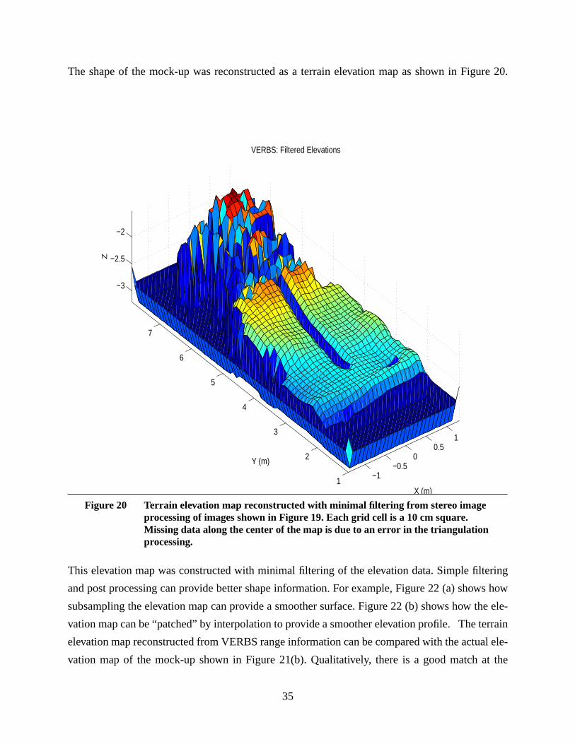
The shape of the mock-up was reconstructed as a terrain elevation map as shown in Figure 20.

This elevation map was constructed with minimal filtering of the elevation data. Simple filtering

and post processing can provide better shape information. For example, Figure 22 (a) shows how

subsampling the elevation map can provide a smoother surface. Figure 22 (b) shows how the ele-

vation map can be “patched” by interpolation to provide a smoother elevation profile. The terrain

elevation map reconstructed from VERBS range information can be compared with the actual ele-

vation map of the mock-up shown in Figure 21(b). Qualitatively, there is a good match at the

Figure 20 Terrain elevation map reconstructed with minimal filtering from stereo imageprocessing of images shown in Figure 19. Each grid cell is a 10 cm square.Missing data along the center of the map is due to an error in the triangulationprocessing.

−1−0.5

00.5

1

1

2

3

4

5

6

7

−3

−2.5

−2

X (m)

VERBS: Filtered Elevations

Y (m)

Z

36

Figure 21 (a) mockup terrain used for ranging experiments. The mockup isapproximately 3 m wide and 5 m long. The structure is made of wooden frameand is covered with a tarp. (b) The shape of the structure is known to within afew cm. We used this as groundtruth to compare the shapes produced by rangedata from stereo vision and ladar.

Figure 22 The elevation map from Figure 20 can be improved by (a) subsampling (gridcells are 20 cm squares), or, (b) interpolation (grid cells remain 10 cm squares).

−3−2

−10

12

0

1

2

3

4

5

6

7

8

−5

−4

−3

−2

−1

X

Terrain Mock−up: Ground Truth

Y

Z

(a) (b)

−1−0.5

00.5

1

1

2

3

4

5

6

7

−3

−2.5

−2

−1.5

X (m)

VERBS: Raw Elevations (0.2m grid)

Y (m)

Z (

m)

−1−0.5

00.5

1

1

2

3

4

5

6

7

−3

−2.5

−2

−1.5

X (m)

VERBS: Patched Elevations

Y (m)

Z

37

lower end of the mock-up (the end closest to the camera) but it degrades towards the higher end

which was furthest from the cameras. Within VERBS any ranges that are determined as unreason-

able are marked as invalid and no range is returned. This missing data is observed in the top left

hand corner of the reconstructed elevation map of Figure 20. The return of no information is bet-

ter than returning grossly inaccurate range information.

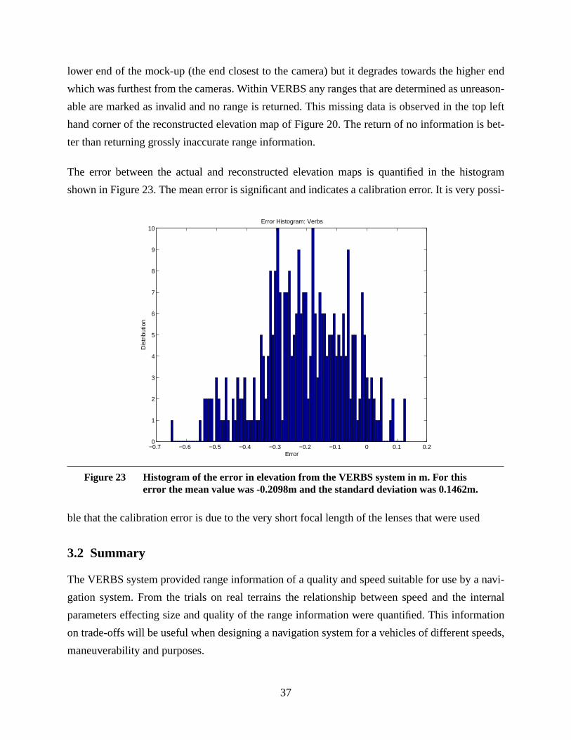
The error between the actual and reconstructed elevation maps is quantified in the histogram

shown in Figure 23. The mean error is significant and indicates a calibration error. It is very possi-

ble that the calibration error is due to the very short focal length of the lenses that were used

3.2 Summary

The VERBS system provided range information of a quality and speed suitable for use by a navi-

gation system. From the trials on real terrains the relationship between speed and the internal

parameters effecting size and quality of the range information were quantified. This information

on trade-offs will be useful when designing a navigation system for a vehicles of different speeds,

maneuverability and purposes.

Figure 23 Histogram of the error in elevation from the VERBS system in m. For thiserror the mean value was -0.2098m and the standard deviation was 0.1462m.

−0.7 −0.6 −0.5 −0.4 −0.3 −0.2 −0.1 0 0.1 0.20

1

2

3

4

5

6

7

8

9

10

Dis

trib

utio

n

Error

Error Histogram: Verbs

38

39

4. Local Navigation

In the course of travelling from one point to another an autonomous vehicle must be able to follow

some global plan and avoid obstacles that were not accounted for in the global plan. That is, the

vehicle must be able to navigate in both a global and local sense. Global navigation is concerned

with the larger movements of the vehicle and local navigation concerned with the details that are

encountered along the way. Often global paths are specified by users as intermediate waypoints

using some apriori but perhaps incomplete and sometimes incorrect information. It is the local

navigation system that must deal with any details that are too small for the global plan to account

for or are unknown. Sometimes global path planning and local navigation are both automatic and

take place at the same time. As the local navigation system discovers obstacles that information is

given to the global path planner that replans taking the new discovery into consideration.

4.1. Overview of Ranger

RANGER is an acronym for Real Time Autonomous Navigator with a Geometric Engine. The

system is an autonomous vehicle control system which specializes in high speed driving in rugged

cross country environments. It has evolved from earlier work on the same problem at CMU and

from the original work on the Autonomous Land Vehicle at CMU and at Hughes Aircraft Corp a

decade ago. Ranger has navigated over distances of 15 autonomous kilometers, moving continu-

ously, and has at times reached speeds of 15 km/hr. The system has been used successfully on a

converted U.S. Army HMMWV and on a specialized Lunar Rover vehicle.

4.1.1. Operational Modes

The system can autonomously seek a predefined goal or it can be configured to supervise remote

or in-situ human drivers. The predefined goal may be a series of points to visit, a continuous path

to follow, a compass heading or a path curvature to follow.

4.1.2. Goal-Seeking

The system can follow a predefined path while avoiding any dangerous hazards along the way or

it can seek a sequence of positions or a particular compass heading. In survival mode, seeking no

particular goal, it will follow the natural contours of the surrounding terrain.

40

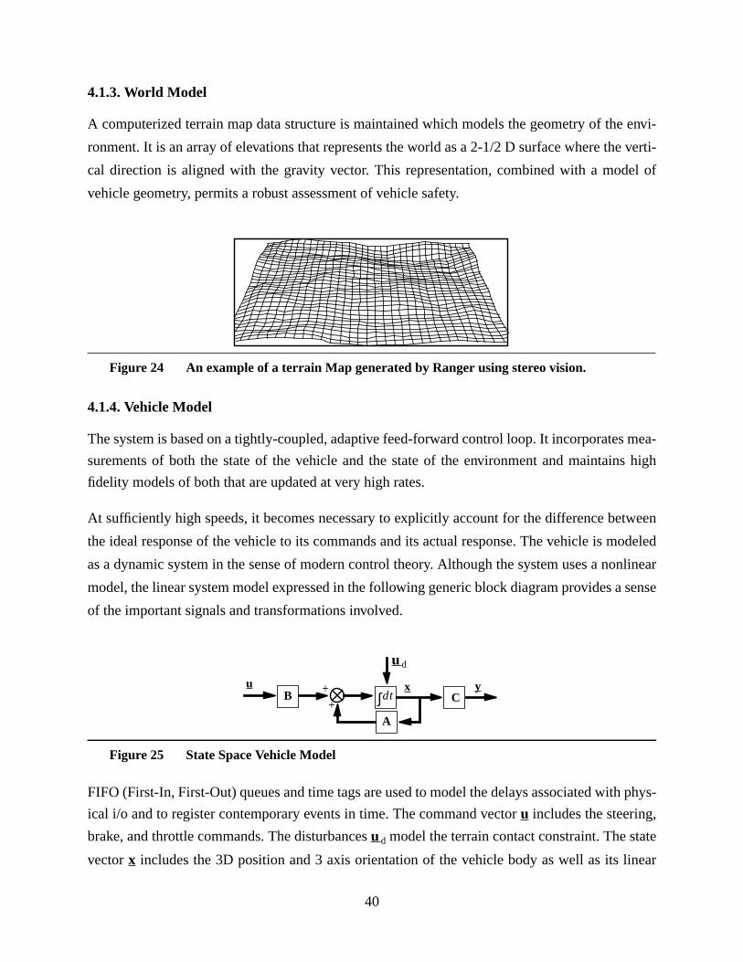
4.1.3. World Model

A computerized terrain map data structure is maintained which models the geometry of the envi-

ronment. It is an array of elevations that represents the world as a 2-1/2 D surface where the verti-

cal direction is aligned with the gravity vector. This representation, combined with a model of

vehicle geometry, permits a robust assessment of vehicle safety.

4.1.4. Vehicle Model

The system is based on a tightly-coupled, adaptive feed-forward control loop. It incorporates mea-

surements of both the state of the vehicle and the state of the environment and maintains high

fidelity models of both that are updated at very high rates.

At sufficiently high speeds, it becomes necessary to explicitly account for the difference between

the ideal response of the vehicle to its commands and its actual response. The vehicle is modeled

as a dynamic system in the sense of modern control theory. Although the system uses a nonlinear

model, the linear system model expressed in the following generic block diagram provides a sense

of the important signals and transformations involved.

FIFO (First-In, First-Out) queues and time tags are used to model the delays associated with phys-

ical i/o and to register contemporary events in time. The command vectoru includes the steering,

brake, and throttle commands. The disturbancesud model the terrain contact constraint. The state

vectorx includes the 3D position and 3 axis orientation of the vehicle body as well as its linear

Figure 24 An example of a terrain Map generated by Ranger using stereo vision.

Figure 25 State Space Vehicle Model

uB

x

++

dt∫A

ud

Cy

41

and angular velocity. The system dynamics matrixA propagates the state of the vehicle forward in

time. The output vectory is a time continuous expression of predicted hazards where each ele-

ment of the vector is a different hazard.

4.1.5. Hazard Assessment

Hazards include regions of unknown terrain, hills that would cause a tip-over, holes and cliffs that

would cause a fall, and small obstacles that would collide with the vehicle wheels or body.

The process of predicting hazardous conditions involves the numerical solution of the equations

of motion while enforcing the constraint that the vehicle remain in contact with the terrain. This

process is a feed-forward process where the current vehicle state furnishes the initial conditions

for numerical integration. The feed-forward approach to hazard assessment imparts high-speed

stability to both goal-seeking and hazard avoidance behaviors.

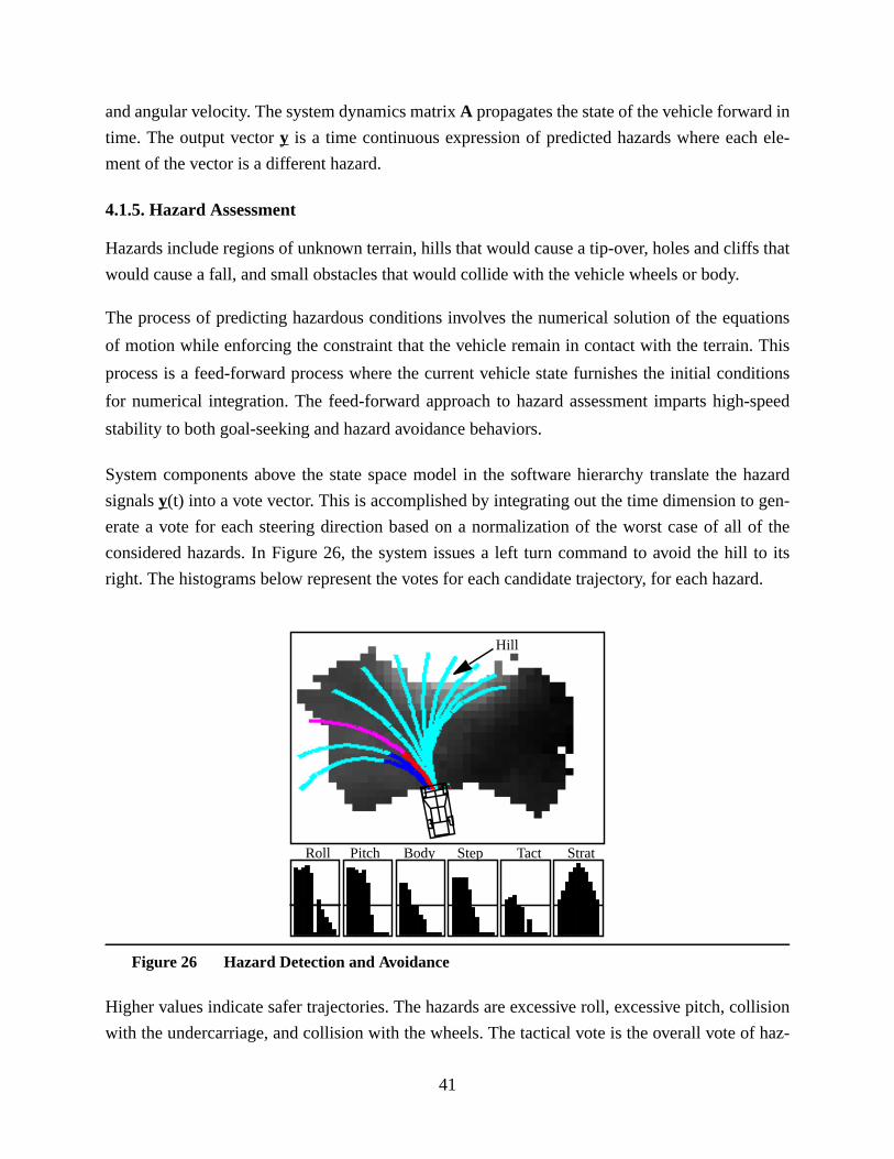
System components above the state space model in the software hierarchy translate the hazard

signalsy(t) into a vote vector. This is accomplished by integrating out the time dimension to gen-

erate a vote for each steering direction based on a normalization of the worst case of all of the

considered hazards. In Figure 26, the system issues a left turn command to avoid the hill to its

right. The histograms below represent the votes for each candidate trajectory, for each hazard.

Higher values indicate safer trajectories. The hazards are excessive roll, excessive pitch, collision

with the undercarriage, and collision with the wheels. The tactical vote is the overall vote of haz-

Figure 26 Hazard Detection and Avoidance

Roll Pitch Body Step Tact Strat

Hill

42

ard avoidance. It wants to turn left. The strategic vote is the goal-seeking vote. Here it votes for

straight ahead.

4.1.6. Arbitration

At times, goal-seeking may cause collision with obstacles because, for example, the goal may be

behind an obstacle. The system incorporates an arbiter which permits obstacle avoidance and

goal-seeking to coexist and to simultaneously influence the behavior of the host vehicle. The arbi-

ter can also integrate the commands of a human driver with the autonomous system.

For the TUGV project three modes of navigation using VERBS were evaluated: (1)Ranger local

navigation, (2)Ranger intermediate navigation using specified waypints and (3)intermediate plan-

ning navigation using a framed quad tree methods. The Ranger system uses a continuous repre-

sentation of world around it. It then calculates the projected roll and pitch for some number of

possible paths. It then compares the relative safety of each potential path as well as the specified

path from the intermediate navigation system. Hopefully the specified path is also a safe path, if

not an arbitration system chooses the path that is the best compromise between the specified path

and maintains an acceptable amount of safety. For navigation using framed quad trees a different

local navigation system called Smarty (cite martial) is used. Smarty uses a discrete view of the

world by dividing the surrounding world up into grid cells, detecting if each of those grid cells is

either occupied or not and then using that grid to plan local paths. The global planner (using

framed quad trees) uses this information to replan its paths and provide smarty with more appro-

priate commands.

The first results presented are for Ranger in local navigation mode alone. In the absence of direc-

tion from a intermediate planner Ranger’s local navigation system attempts to command the vehi-

cle to move straight ahead and, of course, avoiding any obstacles in its way. Next a path is

specified to ranger that will take the vehicle from a starting point, to one intermediate way point

and to a final goal location. To demonstrate ranger’s local navigation capabilities more clearly this

path was purposely chosen to take the vehicle through two obstacles. For demonstrating the inter-

mediate navigation planning system the vehicle started from a point a considerable distance from

the goal. It was unaware of all obstacles and was required to constantly replan its route to the goal.

43

4.2 Experiments with Ranger

For demonstrating the local navigation capabilities alone the vehicle was pointed at various obsta-

cles and in the absence of a desired heading its default heading was straight ahead and directly at

the obstacle. As the vehicle moved close enough for the obstacle to be seen by VERBS ranger’s

local navigation foresees the hazard and the system must alter the path so as to safely avoid the

obstacle. Two types of obstacle were used, the side of a steep wall and a sand pile.

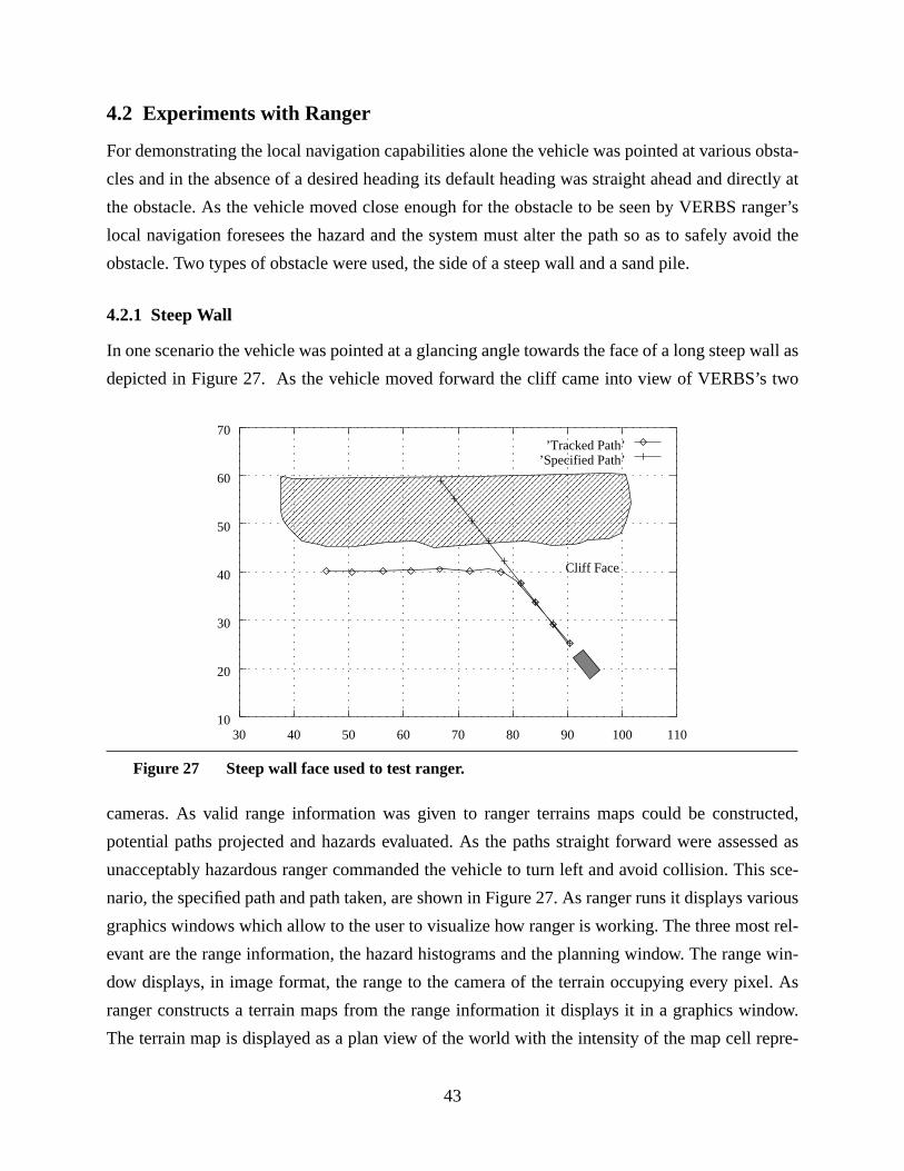
4.2.1 Steep Wall

In one scenario the vehicle was pointed at a glancing angle towards the face of a long steep wall as

depicted in Figure 27. As the vehicle moved forward the cliff came into view of VERBS’s two

cameras. As valid range information was given to ranger terrains maps could be constructed,

potential paths projected and hazards evaluated. As the paths straight forward were assessed as

unacceptably hazardous ranger commanded the vehicle to turn left and avoid collision. This sce-

nario, the specified path and path taken, are shown in Figure 27. As ranger runs it displays various

graphics windows which allow to the user to visualize how ranger is working. The three most rel-

evant are the range information, the hazard histograms and the planning window. The range win-

dow displays, in image format, the range to the camera of the terrain occupying every pixel. As

ranger constructs a terrain maps from the range information it displays it in a graphics window.

The terrain map is displayed as a plan view of the world with the intensity of the map cell repre-

Figure 27 Steep wall face used to test ranger.

�������������������������������������������������������������������������������������

�������������������������������������������������������������������������������������’Specified Path’

’Tracked Path’

10

20

30

40

50

60

70

30 40 50 60 70 80 90 100 110

Cliff Face

44

senting that cell’s elevation. The vehicle’s location as well as the selected path are also shown in

the terrain map window. The hazard histograms display the safety of each possible path. For each

criteria (roll, pitch and unknown terrain) the center histogram bar represents the straight ahead

path and the bars to the left and right of the center represent paths to the left and right for the vehi-

cle. Each path is evaluated by projecting the vehicle state along each path in the terrain map.

Excessive vehicle roll, pitch or traversal across unknown terrain represent unsafe situations. The

higher the histogram bar value the safer the path. The horizontal line represents the safety thresh-

old below which no path is considered safe.

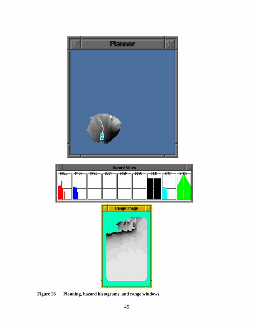
For this cliff face scenario the high elevation of the portion of the cliff face that is in view is seen

in both the range image (cliff face is forward and to the right of the vehicle) and the terrain map of

Figure 28. The hazard histograms indicate excessive roll and pitch would occur for paths directly

forward and to the right while paths turning to the left are shown as safe. The path taken by the

vehicle is superimposed upon the terrain map in front of the wire frame model of the vehicle. The

vehicle moved forward along this path until the cliff face was no longer in front and it could safely

follow its default specified path (straight ahead). The specified and actual paths resembled those

shown in Figure 27.

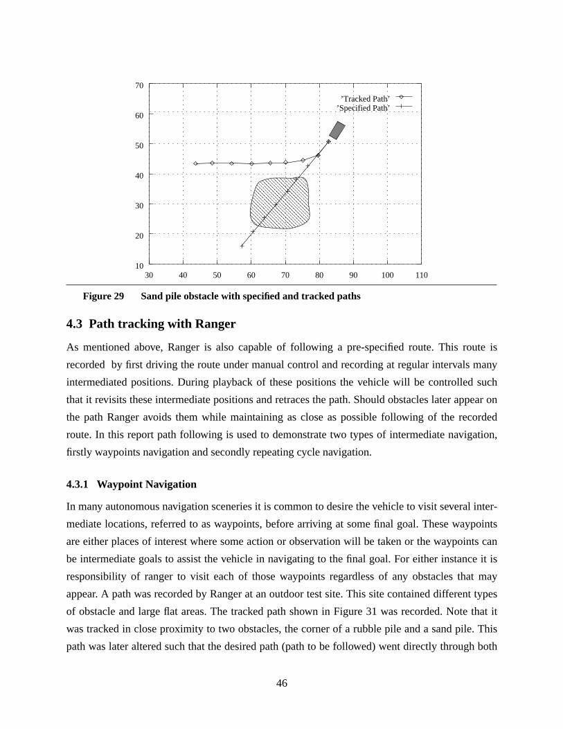
4.2.2 Sand Pile

In the next scenario the vehicle was set pointing directly at a pile of sand that was about 12 feet in

diameter and about 7 feet in height. The vehicle position, sand pile and specified and actual paths

resembled those shown in Figure 29.

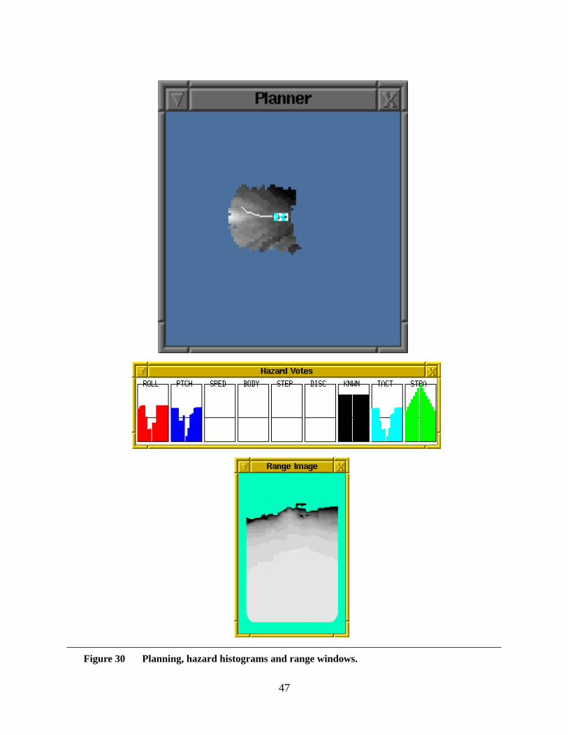
The hazard votes histograms shown in Figure 30 display the safety with regard to roll, pitch and

the amount of unknown terrain that would be crossed for each of the vehicles potential paths.

These histograms indicate that excessive roll and pitch will occur for paths that are projected

thought the sand pile including the default desired path. Safe paths are indicated as those that

avoid the pile by turning to the left or to the right. The safest path as chosen by ranger is superim-

posed on the terrain map of Figure 30. As the vehicle moved its desired path and actual paths

resembled those shown inFigure 29. Once the vehicle avoided the sand pile it resumed its desired

heading (straight ahead).

45

Figure 28 Planning, hazard histograms, and range windows.

46

4.3 Path tracking with Ranger

As mentioned above, Ranger is also capable of following a pre-specified route. This route is

recorded by first driving the route under manual control and recording at regular intervals many

intermediated positions. During playback of these positions the vehicle will be controlled such

that it revisits these intermediate positions and retraces the path. Should obstacles later appear on

the path Ranger avoids them while maintaining as close as possible following of the recorded

route. In this report path following is used to demonstrate two types of intermediate navigation,

firstly waypoints navigation and secondly repeating cycle navigation.

4.3.1 Waypoint Navigation

In many autonomous navigation sceneries it is common to desire the vehicle to visit several inter-

mediate locations, referred to as waypoints, before arriving at some final goal. These waypoints

are either places of interest where some action or observation will be taken or the waypoints can

be intermediate goals to assist the vehicle in navigating to the final goal. For either instance it is

responsibility of ranger to visit each of those waypoints regardless of any obstacles that may

appear. A path was recorded by Ranger at an outdoor test site. This site contained different types

of obstacle and large flat areas. The tracked path shown in Figure 31 was recorded. Note that it

was tracked in close proximity to two obstacles, the corner of a rubble pile and a sand pile. This

path was later altered such that the desired path (path to be followed) went directly through both

Figure 29 Sand pile obstacle with specified and tracked paths

������������������������������

������������������������������

10

20

30

40

50

60

70

30 40 50 60 70 80 90 100 110

’Tracked Path’’Specified Path’

47

Figure 30 Planning, hazard histograms and range windows.

48

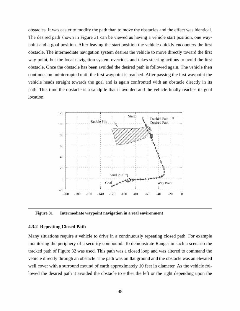
obstacles. It was easier to modify the path than to move the obstacles and the effect was identical.

The desired path shown in Figure 31 can be viewed as having a vehicle start position, one way-

point and a goal position. After leaving the start position the vehicle quickly encounters the first

obstacle. The intermediate navigation system desires the vehicle to move directly toward the first

way point, but the local navigation system overrides and takes steering actions to avoid the first

obstacle. Once the obstacle has been avoided the desired path is followed again. The vehicle then

continues on uninterrupted until the first waypoint is reached. After passing the first waypoint the

vehicle heads straight towards the goal and is again confronted with an obstacle directly in its

path. This time the obstacle is a sandpile that is avoided and the vehicle finally reaches its goal

location.

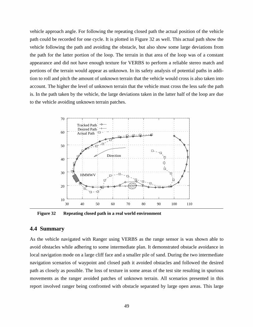
4.3.2 Repeating Closed Path

Many situations require a vehicle to drive in a continuously repeating closed path. For example

monitoring the periphery of a security compound. To demonstrate Ranger in such a scenario the

tracked path of Figure 32 was used. This path was a closed loop and was altered to command the

vehicle directly through an obstacle. The path was on flat ground and the obstacle was an elevated

well cover with a surround mound of earth approximately 10 feet in diameter. As the vehicle fol-

lowed the desired path it avoided the obstacle to either the left or the right depending upon the

Figure 31 Intermediate waypoint navigation in a real environment

�����������������������������������

�����������������������������������

��������

-20

0

20

40

60

80

100

120

-200 -180 -160 -140 -120 -100 -80 -60 -40 -20 0

Tracked PathDesired Path

Start

Goal Way Point

Sand Pile

Rubble Pile

49

vehicle approach angle. For following the repeating closed path the actual position of the vehicle

path could be recorded for one cycle. It is plotted in Figure 32 as well. This actual path show the

vehicle following the path and avoiding the obstacle, but also show some large deviations from

the path for the latter portion of the loop. The terrain in that area of the loop was of a constant

appearance and did not have enough texture for VERBS to perform a reliable stereo match and

portions of the terrain would appear as unknown. In its safety analysis of potential paths in addi-

tion to roll and pitch the amount of unknown terrain that the vehicle would cross is also taken into

account. The higher the level of unknown terrain that the vehicle must cross the less safe the path

is. In the path taken by the vehicle, the large deviations taken in the latter half of the loop are due

to the vehicle avoiding unknown terrain patches.

4.4 Summary

As the vehicle navigated with Ranger using VERBS as the range sensor is was shown able to

avoid obstacles while adhering to some intermediate plan. It demonstrated obstacle avoidance in

local navigation mode on a large cliff face and a smaller pile of sand. During the two intermediate

navigation scenarios of waypoint and closed path it avoided obstacles and followed the desired

path as closely as possible. The loss of texture in some areas of the test site resulting in spurious

movements as the ranger avoided patches of unknown terrain. All scenarios presented in this

report involved ranger being confronted with obstacle separated by large open areas. This large

Figure 32 Repeating closed path in a real world environment

������������

������������

Actual Path

Tracked PathDesired Path

10

20

30

40

50

60

70

30 40 50 60 70 80 90 100 110

Direction

HMMWV

50

distance between obstacles prevented the avoidance movements from previous obstacles com-

pounding the difficulty of the movements required to avoid the next obstacle. Difficulties in navi-

gating areas with a high obstacle density were noticed.

51

5. Global Navigation

Path planning for a mobile is typically stated as getting from one place to another. The robot must

successfully navigate around obstacles, reach its goal and do so efficiently. Outdoor environments

pose special challenges over the structured world that is often found indoors. Not only must a

robot avoid colliding with an obstacle such as a rock, it must also avoid falling into a pit or ravine

and avoid travel on terrain that would cause it to tip over. Vast areas have their own associated

issues. Such areas typically have large open areas where a robot might travel freely and are

sparsely populated with obstacles. However, the range of obstacles that can interfere with the

robot’s passage is large— the robot must still avoid a rock as well as go around a mountain. Vast

areas are unlikely to be mapped at high resolution a priori and hence the robot must explore as it

goes, incorporating newly discovered information into its database. Hence, the solution must be

incrementalby necessity. Another challenge is dealing with a large amount of information and a

complex model (our autonomous vehicle is a three degree of freedom, non-linear, non-holonomic

system). Taken as a single problem, so much information must be processed to determine the

robot’s next action that it is not possible for the robot to perform at any reasonable rate. We deal

with this issue by using alayered approach to navigation.

As mentioned earlier, we have adopted the approach of decomposing navigation into two levels—

local and global. The job of local planning is to avoid obstacles, reacting to sensory data as

quickly as possible while driving towards a subgoal [7][8]. A more deliberative process, operating

at a coarser resolution of information is used to decide how best select the subgoals such that the

goal can be reached. This approach has been used successfully in the past in several systems at

Carnegie Mellon [7][15]. In this paper we concentrate the discussion on global planning.

Approaches to path planning for mobile robots can be broadly classified into two categories—

those that use exact representations of the world (e.g. [17]), and those that use a discretized repre-

sentation (e.g. [6][9]). The main advantage of discretization is that the computational complexity

of path planning can be controlled by adjusting the cell size. In contrast, the computational com-

plexity of exact methods is a function of the number of obstacles and/or the number of obstacle

facets, which we cannot normally control. Even with discretized worlds path planning can be

computationally expensive and on-line performance is typically achieved by use of specialized

computing hardware as in [6][9]. By comparison the proposed method requires general purpose

computing only. This is made possible by precomputing an optimal path off-line given whatever a

52

priori map is available, and then optimally modifying the path as new map information becomes

available, on-line.

Methods that use uniform grid representations must allocate large amounts of memory for regions

that may never be traversed, or contain any obstacles. Efficiency in map representation can be

obtained by the use of quadtrees, but at a cost of optimality. Recently, a new data structure called

a framed quadtreehas been suggested as means to overcome some of the issues related to the use

of quadtrees[5]. We have used this data structure to extend an existing path planner that has in the

past used uniform (regular) grid cells to represent terrain. This path planner, D* [13][14] has been

shown to be optimal in cases where the environment is incrementally discovered.

In this paper we discuss the advantages and implications of using framed quadtrees with D*. We

present results of the path planner operating in simulated fractal worlds and results from imple-

mentation on an autonomous jeep.

5.1 Map Representation

Apart from the fact that discretization of space allows for control over the complexity of path

planning, it also provides a flexible representation for obstacles and cost maps, and eases imple-

mentation. One method of cell decomposition is to tessellate space into equal sized cells each of

which is connected to its neighbors with four or eight arcs. This method, however, has two draw-

backs: resulting paths can be suboptimal and memory requirements high. Quadtrees address the

latter problem, while framed quadtrees address both problems, especially in sparse environments.

5.1.1 Regular Grids

Regular grids represent space inefficiently. Natural terrains are usually sparsely populated and are

often not completely known in advance. In the absence of map information unknown environ-

ments are encoded sparsely during initial exploration and many areas remain sparsely populated

even during execution. Many equally sized cells are needed to encode these empty areas making

search expensive since more cells are processed than actually needed. Moreover, regular grids

allow only eight angles for direction, resulting in abrupt changes in path direction and an inability,

in some cases, to generate a straight path through empty areas (Figure 33a). It is possible to

smooth such jagged paths, but there is no guarantee that the smoothed path will converge to the

truly optimal path.

53

5.1.2 Quadtrees

One way to reduce memory requirements is to use a quadtree instead of a regular grid. A quadtree

[11][12] is based on the successive subdivision of region into four equally sized quadrants. A

region is recursively subdivided until either a subregion free of obstacles is found or the smallest

grid cell is reached. Quadtrees allow efficient partitioning of the environment since single cells

can be used to encode large empty regions. However, paths generated by quadtrees are suboptimal

because they are constrained to segments between the centers of the cells. Figure 33b shows an

example path generated using a quadtree.

5.1.3 Framed Quadtrees

To remedy the above problem, we have used a modified data structure in which cells of the high-

est resolution are added around the perimeter of each quadtree region. This augmented representa-

tion is called aframed quadtree. A path generated using this representation is shown in Figure

33c. The small grey rectangles around the cells are the border cells of each quadrant. This repre-

sentation permits many angles of direction, instead of just eight angles as in the case of regular

grids. A path can be constructed between two border cells lying far away from each other. Most

importantly, the paths generated more closely approximate optimal paths.

The drawback of using framed quadtrees is that they can require more memory than regular grids

in uniformly, highly cluttered environments because of the overhead involved in the book-keep-

ing.

5.2 Incremental Planning

Unstructured outdoor environments are often not only sparse but also typically only partial maps

are available. If complete and accurate maps were available, it would be sufficient to use A* [10]

once to search the map and produce a path. The robot could simply follow this path during its

traverse. Furthermore, errors in control and perception often introduce erroneous and changing

information. Ideally, the robot should gather new information about the environment, and effi-

ciently replan new paths based on this new information. In these partially known environments, a

traverse can be achieved by incrementally incorporating information as it becomes available.

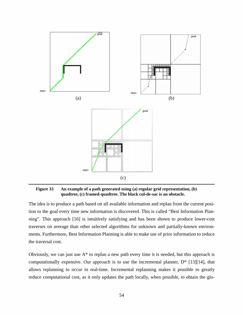
54

The idea is to produce a path based on all available information and replan from the current posi-

tion to the goal every time new information is discovered. This is called “Best Information Plan-

ning”. This approach [16] is intuitively satisfying and has been shown to produce lower-cost

traverses on average than other selected algorithms for unknown and partially-known environ-

ments. Furthermore, Best Information Planning is able to make use of prior information to reduce

the traversal cost.

Obviously, we can just use A* to replan a new path every time it is needed, but this approach is

computationally expensive. Our approach is to use the incremental planner, D* [13][14], that

allows replanning to occur in real-time. Incremental replanning makes it possible to greatly

reduce computational cost, as it only updates the path locally, when possible, to obtain the glo-

Figure 33 An example of a path generated using (a) regular grid representation, (b)quadtree, (c) framed-quadtree. The black cul-de-sac is an obstacle.

start

goal

start

goal

start

goal

(a) (b)

(c)

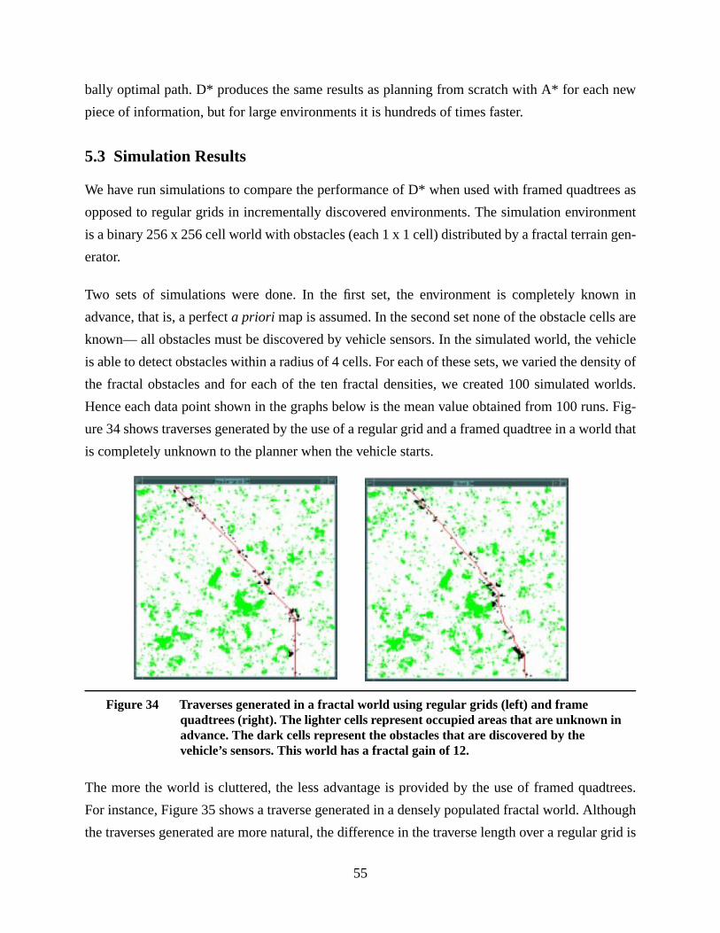
55

bally optimal path. D* produces the same results as planning from scratch with A* for each new

piece of information, but for large environments it is hundreds of times faster.

5.3 Simulation Results

We have run simulations to compare the performance of D* when used with framed quadtrees as

opposed to regular grids in incrementally discovered environments. The simulation environment

is a binary 256 x 256 cell world with obstacles (each 1 x 1cell) distributed by a fractal terrain gen-

erator.

Two sets of simulations were done. In the first set, the environment is completely known in

advance, that is, a perfecta priori map is assumed. In the second set none of the obstacle cells are

known— all obstacles must be discovered by vehicle sensors. In the simulated world, the vehicle

is able to detect obstacles within a radius of 4 cells. For each of these sets, we varied the density of

the fractal obstacles and for each of the ten fractal densities, we created 100 simulated worlds.

Hence each data point shown in the graphs below is the mean value obtained from 100 runs. Fig-

ure 34 shows traverses generated by the use of a regular grid and a framed quadtree in a world that

is completely unknown to the planner when the vehicle starts.

The more the world is cluttered, the less advantage is provided by the use of framed quadtrees.

For instance, Figure 35 shows a traverse generated in a densely populated fractal world. Although

the traverses generated are more natural, the difference in the traverse length over a regular grid is

Figure 34 Traverses generated in a fractal world using regular grids (left) and framequadtrees (right). The lighter cells represent occupied areas that are unknown inadvance. The dark cells represent the obstacles that are discovered by thevehicle’s sensors. This world has a fractal gain of 12.

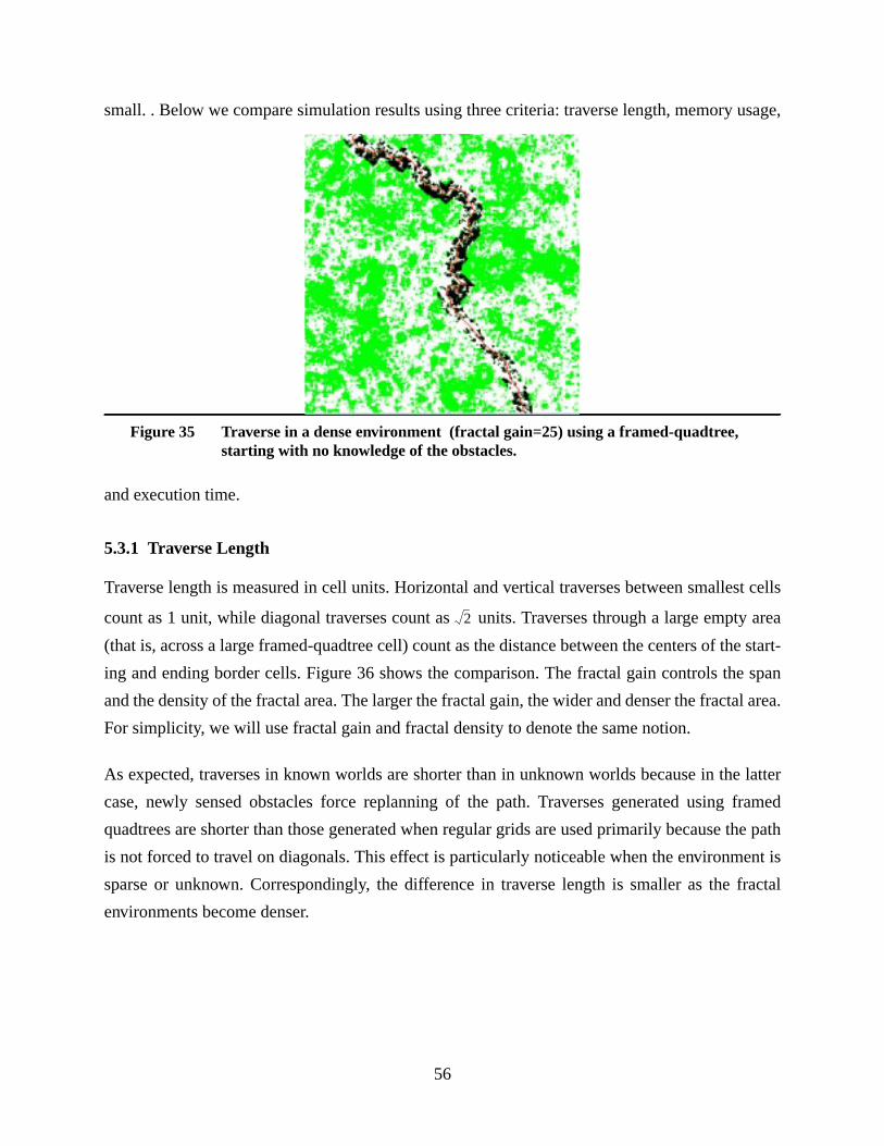
56

small. . Below we compare simulation results using three criteria: traverse length, memory usage,

and execution time.

5.3.1 Traverse Length

Traverse length is measured in cell units. Horizontal and vertical traverses between smallest cells

count as 1 unit, while diagonal traverses count as units. Traverses through a large empty area

(that is, across a large framed-quadtree cell) count as the distance between the centers of the start-

ing and ending border cells. Figure 36 shows the comparison. The fractal gain controls the span

and the density of the fractal area. The larger the fractal gain, the wider and denser the fractal area.

For simplicity, we will use fractal gain and fractal density to denote the same notion.

As expected, traverses in known worlds are shorter than in unknown worlds because in the latter

case, newly sensed obstacles force replanning of the path. Traverses generated using framed

quadtrees are shorter than those generated when regular grids are used primarily because the path

is not forced to travel on diagonals. This effect is particularly noticeable when the environment is

sparse or unknown. Correspondingly, the difference in traverse length is smaller as the fractal

environments become denser.

Figure 35 Traverse in a dense environment (fractal gain=25) using a framed-quadtree,starting with no knowledge of the obstacles.

2

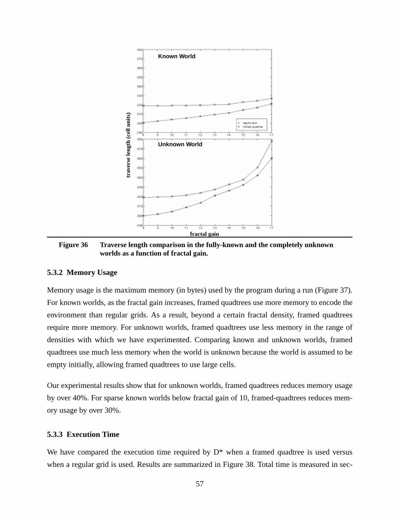
57

5.3.2 Memory Usage

Memory usage is the maximum memory (in bytes) used by the program during a run (Figure 37).

For known worlds, as the fractal gain increases, framed quadtrees use more memory to encode the

environment than regular grids. As a result, beyond a certain fractal density, framed quadtrees

require more memory. For unknown worlds, framed quadtrees use less memory in the range of

densities with which we have experimented. Comparing known and unknown worlds, framed

quadtrees use much less memory when the world is unknown because the world is assumed to be

empty initially, allowing framed quadtrees to use large cells.

Our experimental results show that for unknown worlds, framed quadtrees reduces memory usage

by over 40%. For sparse known worlds below fractal gain of 10, framed-quadtrees reduces mem-

ory usage by over 30%.

5.3.3 Execution Time

We have compared the execution time required by D* when a framed quadtree is used versus

when a regular grid is used. Results are summarized in Figure 38. Total time is measured in sec-

Figure 36 Traverse length comparison in the fully-known and the completely unknownworlds as a function of fractal gain.

trav

erse

leng

th (

cell

units

)

fractal gain

Known World

Unknown World

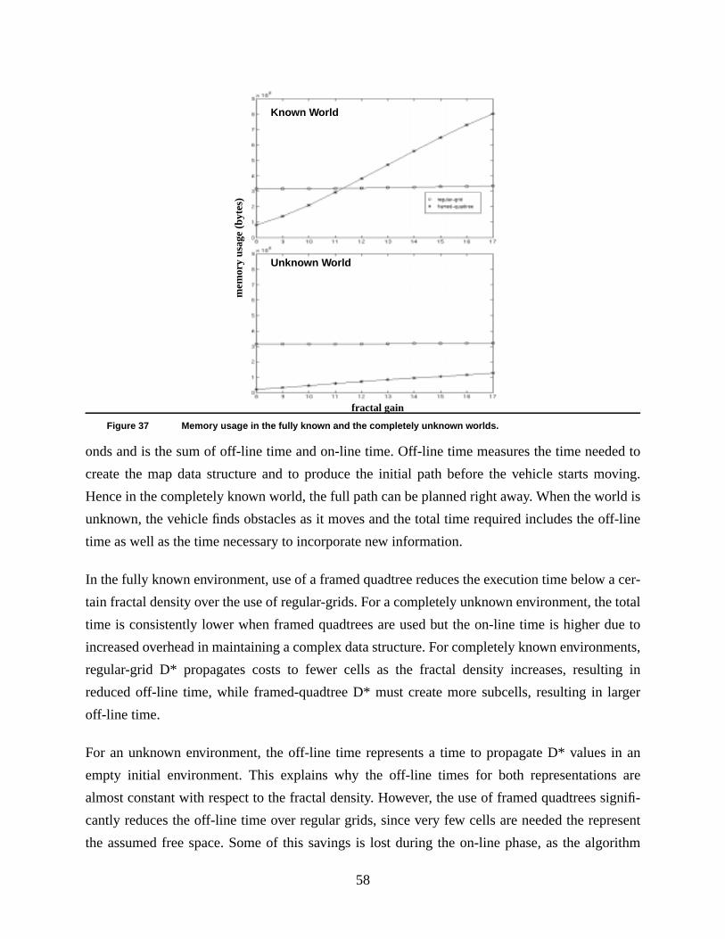
58

onds and is the sum of off-line time and on-line time. Off-line time measures the time needed to

create the map data structure and to produce the initial path before the vehicle starts moving.

Hence in the completely known world, the full path can be planned right away. When the world is

unknown, the vehicle finds obstacles as it moves and the total time required includes the off-line

time as well as the time necessary to incorporate new information.

In the fully known environment, use of a framed quadtree reduces the execution time below a cer-

tain fractal density over the use of regular-grids. For a completely unknown environment, the total

time is consistently lower when framed quadtrees are used but the on-line time is higher due to

increased overhead in maintaining a complex data structure. For completely known environments,

regular-grid D* propagates costs to fewer cells as the fractal density increases, resulting in

reduced off-line time, while framed-quadtree D* must create more subcells, resulting in larger

off-line time.

For an unknown environment, the off-line time represents a time to propagate D* values in an

empty initial environment. This explains why the off-line times for both representations are

almost constant with respect to the fractal density. However, the use of framed quadtrees signifi-

cantly reduces the off-line time over regular grids, since very few cells are needed the represent

the assumed free space. Some of this savings is lost during the on-line phase, as the algorithm

Figure 37 Memory usage in the fully known and the completely unknown worlds.

mem

ory

usag

e (b

ytes

)

Known World

Unknown World

fractal gain

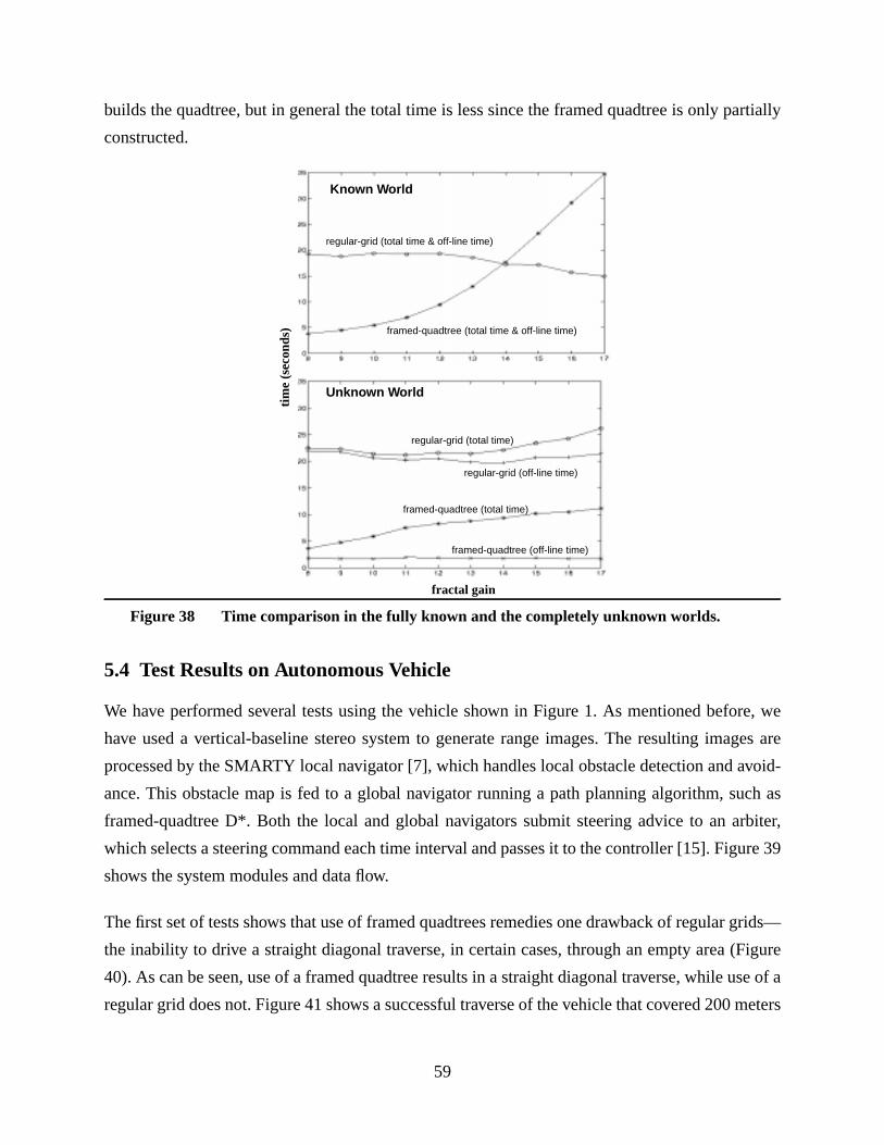
59

builds the quadtree, but in general the total time is less since the framed quadtree is only partially

constructed.

5.4 Test Results on Autonomous Vehicle

We have performed several tests using the vehicle shown in Figure 1. As mentioned before, we

have used a vertical-baseline stereo system to generate range images. The resulting images are

processed by the SMARTY local navigator [7], which handles local obstacle detection and avoid-

ance. This obstacle map is fed to a global navigator running a path planning algorithm, such as

framed-quadtree D*. Both the local and global navigators submit steering advice to an arbiter,

which selects a steering command each time interval and passes it to the controller [15]. Figure 39

shows the system modules and data flow.

The first set of tests shows that use of framed quadtrees remedies one drawback of regular grids—

the inability to drive a straight diagonal traverse, in certain cases, through an empty area (Figure

40). As can be seen, use of a framed quadtree results in a straight diagonal traverse, while use of a

regular grid does not. Figure 41 shows a successful traverse of the vehicle that covered 200 meters

Figure 38 Time comparison in the fully known and the completely unknown worlds.

time

(sec

onds

)

fractal gain

Known World

Unknown World

regular-grid (total time)

regular-grid (off-line time)

framed-quadtree (total time)

framed-quadtree (off-line time)

regular-grid (total time & off-line time)

framed-quadtree (total time & off-line time)

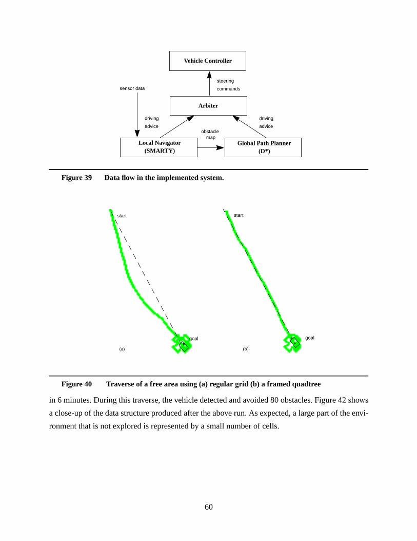
60

in 6 minutes. During this traverse, the vehicle detected and avoided 80 obstacles. Figure 42 shows

a close-up of the data structure produced after the above run. As expected, a large part of the envi-

ronment that is not explored is represented by a small number of cells.

Figure 39 Data flow in the implemented system.

Figure 40 Traverse of a free area using (a) regular grid (b) a framed quadtree

Vehicle Controller

Arbiter

Local Navigator Global Path Planner(SMARTY) (D*)

steering

commands

driving

advice

driving

advice

sensor data

obstacle map

start

goal

start

goal

(b)(a)

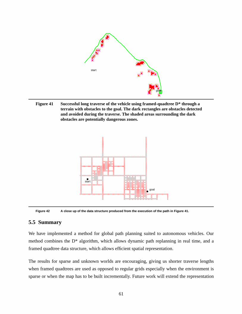
61

5.5 Summary

We have implemented a method for global path planning suited to autonomous vehicles. Our

method combines the D* algorithm, which allows dynamic path replanning in real time, and a

framed quadtree data structure, which allows efficient spatial representation.

The results for sparse and unknown worlds are encouraging, giving us shorter traverse lengths

when framed quadtrees are used as opposed to regular grids especially when the environment is

sparse or when the map has to be built incrementally. Future work will extend the representation

Figure 41 Successful long traverse of the vehicle using framed-quadtree D* through aterrain with obstacles to the goal. The dark rectangles are obstacles detectedand avoided during the traverse. The shaded areas surrounding the darkobstacles are potentially dangerous zones.

Figure 42 A close up of the data structure produced from the execution of the path in Figure 41.

start

goal

goal

start

62

to continuously varying worlds as opposed to the binary worlds considered to date. Additionally,

we will show the utility of this method in partially known environments, that is where maps exist

but at a coarser scale.

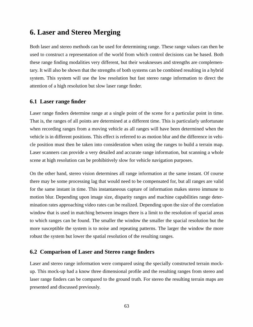
63

6. Laser and Stereo Merging

Both laser and stereo methods can be used for determining range. These range values can then be

used to construct a representation of the world from which control decisions can be based. Both

these range finding modalities very different, but their weaknesses and strengths are complemen-

tary. It will also be shown that the strengths of both systems can be combined resulting in a hybrid

system. This system will use the low resolution but fast stereo range information to direct the

attention of a high resolution but slow laser range finder.

6.1 Laser range finder

Laser range finders determine range at a single point of the scene for a particular point in time.

That is, the ranges of all points are determined at a different time. This is particularly unfortunate

when recording ranges from a moving vehicle as all ranges will have been determined when the

vehicle is in different positions. This effect is referred to as motion blur and the difference in vehi-

cle position must then be taken into consideration when using the ranges to build a terrain map.

Laser scanners can provide a very detailed and accurate range information, but scanning a whole

scene at high resolution can be prohibitively slow for vehicle navigation purposes.

On the other hand, stereo vision determines all range information at the same instant. Of course

there may be some processing lag that would need to be compensated for, but all ranges are valid

for the same instant in time. This instantaneous capture of information makes stereo immune to

motion blur. Depending upon image size, disparity ranges and machine capabilities range deter-

mination rates approaching video rates can be realized. Depending upon the size of the correlation

window that is used in matching between images there is a limit to the resolution of spacial areas

to which ranges can be found. The smaller the window the smaller the spacial resolution but the

more susceptible the system is to noise and repeating patterns. The larger the window the more

robust the system but lower the spatial resolution of the resulting ranges.

6.2 Comparison of Laser and Stereo range finders

Laser and stereo range information were compared using the specially constructed terrain mock-

up. This mock-up had a know three dimensional profile and the resulting ranges from stereo and

laser range finders can be compared to the ground truth. For stereo the resulting terrain maps are

presented and discussed previously.

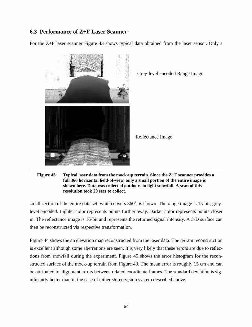
64

6.3 Performance of Z+F Laser Scanner

For the Z+F laser scanner Figure 43 shows typical data obtained from the laser sensor. Only a

small section of the entire data set, which covers 360˚, is shown. The range image is 15-bit, grey-

level encoded. Lighter color represents points further away. Darker color represents points closer

in. The reflectance image is 16-bit and represents the returned signal intensity. A 3-D surface can

then be reconstructed via respective transformation.

Figure 44 shows the an elevation map reconstructed from the laser data. The terrain reconstruction

is excellent although some aberrations are seen. It is very likely that these errors are due to reflec-

tions from snowfall during the experiment. Figure 45 shows the error histogram for the recon-

structed surface of the mock-up terrain from Figure 43. The mean error is roughly 15 cm and can

be attributed to alignment errors between related coordinate frames. The standard deviation is sig-

nificantly better than in the case of either stereo vision system described above.

Figure 43 Typical laser data from the mock-up terrain. Since the Z+F scanner provides afull 360 horizontal field-of-view, only a small portion of the entire image isshown here. Data was collected outdoors in light snowfall. A scan of thisresolution took 20 secs to collect.

Grey-level encoded Range Image

Reflectance Image

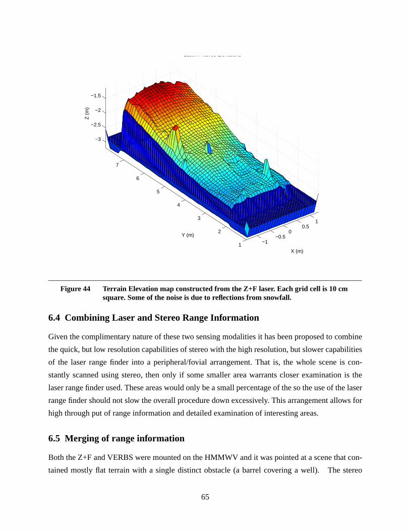
65

6.4 Combining Laser and Stereo Range Information

Given the complimentary nature of these two sensing modalities it has been proposed to combine

the quick, but low resolution capabilities of stereo with the high resolution, but slower capabilities

of the laser range finder into a peripheral/fovial arrangement. That is, the whole scene is con-

stantly scanned using stereo, then only if some smaller area warrants closer examination is the

laser range finder used. These areas would only be a small percentage of the so the use of the laser

range finder should not slow the overall procedure down excessively. This arrangement allows for

high through put of range information and detailed examination of interesting areas.

6.5 Merging of range information

Both the Z+F and VERBS were mounted on the HMMWV and it was pointed at a scene that con-

tained mostly flat terrain with a single distinct obstacle (a barrel covering a well). The stereo

Figure 44 Terrain Elevation map constructed from the Z+F laser. Each grid cell is 10 cmsquare. Some of the noise is due to reflections from snowfall.

−1−0.5

00.5

1

1

2

3

4

5

6

7

−3

−2.5

−2

−1.5

X (m)

Laser: Filtered Elevations

Y (m)

Z (

m)

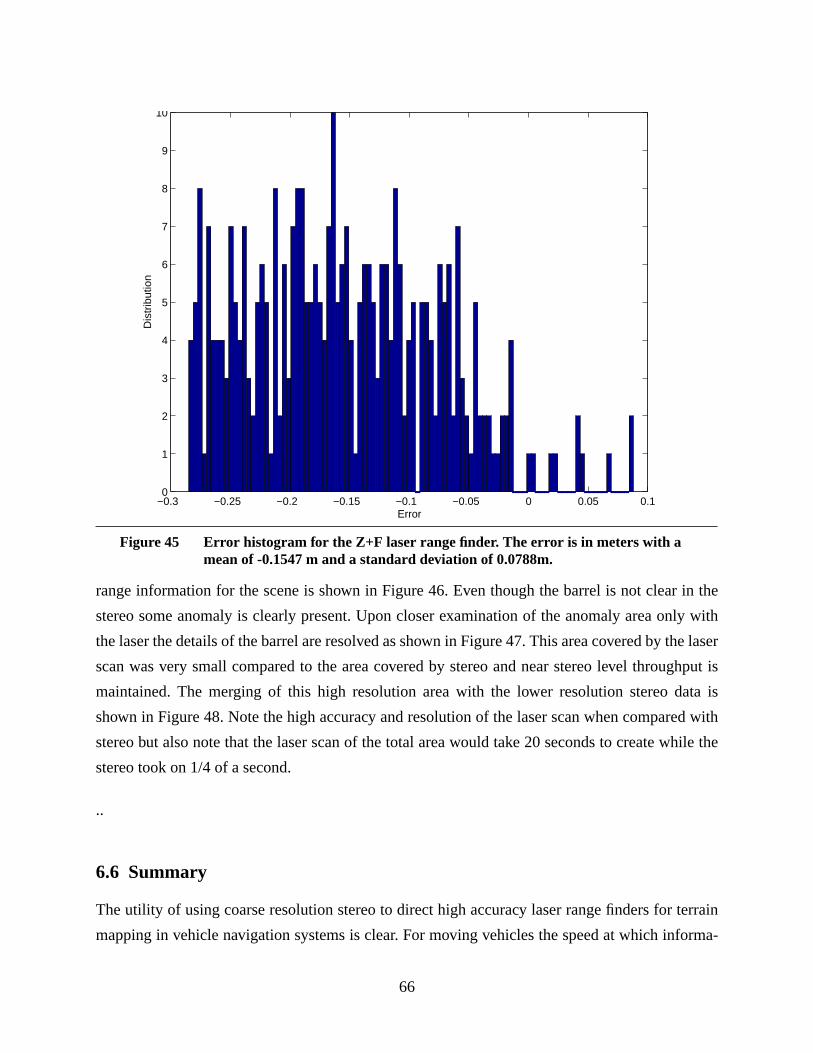
66

range information for the scene is shown in Figure 46. Even though the barrel is not clear in the

stereo some anomaly is clearly present. Upon closer examination of the anomaly area only with

the laser the details of the barrel are resolved as shown in Figure 47. This area covered by the laser

scan was very small compared to the area covered by stereo and near stereo level throughput is

maintained. The merging of this high resolution area with the lower resolution stereo data is

shown in Figure 48. Note the high accuracy and resolution of the laser scan when compared with

stereo but also note that the laser scan of the total area would take 20 seconds to create while the

stereo took on 1/4 of a second.

..

6.6 Summary

The utility of using coarse resolution stereo to direct high accuracy laser range finders for terrain

mapping in vehicle navigation systems is clear. For moving vehicles the speed at which informa-

Figure 45 Error histogram for the Z+F laser range finder. The error is in meters with amean of -0.1547 m and a standard deviation of 0.0788m.

−0.3 −0.25 −0.2 −0.15 −0.1 −0.05 0 0.05 0.10

1

2

3

4

5

6

7

8

9

10

Dis

trib

utio

n

Error

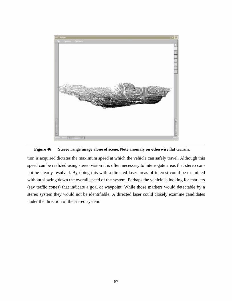
67

tion is acquired dictates the maximum speed at which the vehicle can safely travel. Although this

speed can be realized using stereo vision it is often necessary to interrogate areas that stereo can-

not be clearly resolved. By doing this with a directed laser areas of interest could be examined

without slowing down the overall speed of the system. Perhaps the vehicle is looking for markers

(say traffic cones) that indicate a goal or waypoint. While those markers would detectable by a

stereo system they would not be identifiable. A directed laser could closely examine candidates

under the direction of the stereo system.

Figure 46 Stereo range image alone of scene. Note anomaly on otherwise flat terrain.

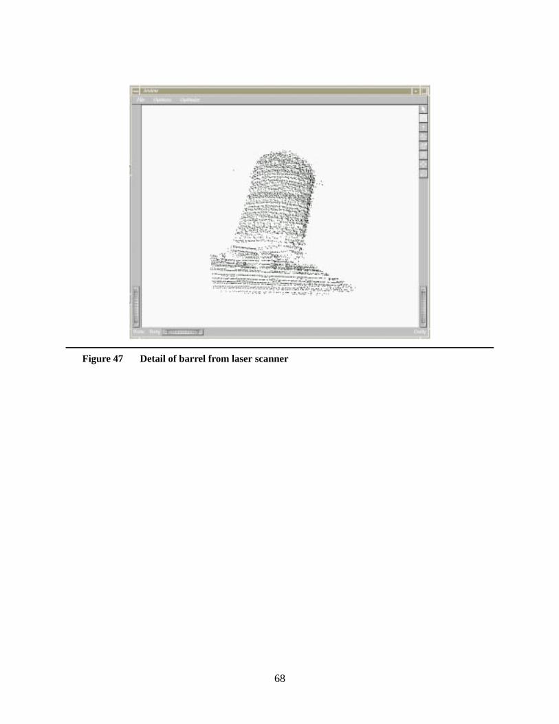
68

Figure 47 Detail of barrel from laser scanner

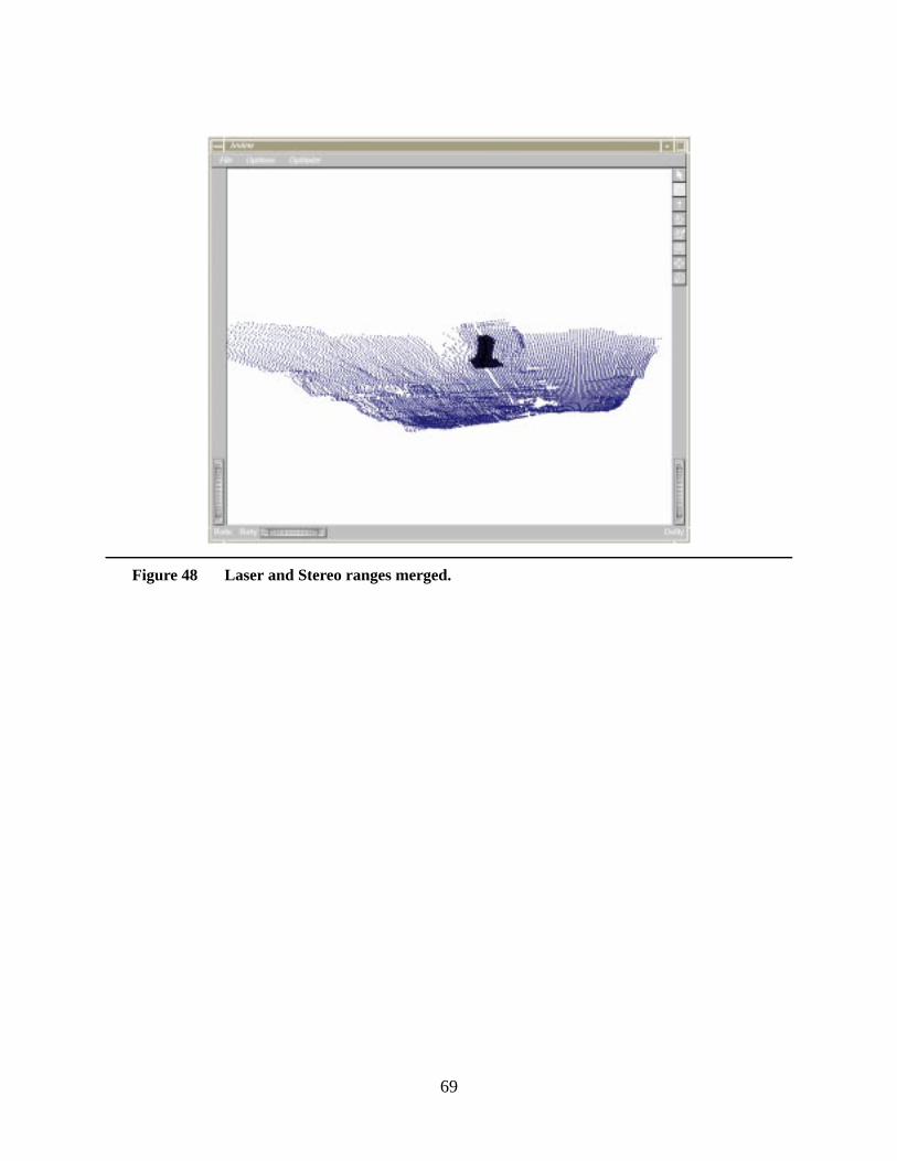
69

Figure 48 Laser and Stereo ranges merged.

70

71

7. Conclusion

In this report the complete system for navigation of a HMMWV in natural outdoor terrains over

long distances in unknown territory has been developed and presented. The system was able to

perceive the terrain in front of the vehicle using a wide field of view vertical baseline stereo vision

system. The calibration and rectification procedures that were developed successful removed the

barrel distortion and misalignment from the images. The VERBS system provided was able to

provide very good range information and allowed for autonomous vehicle navigation. The trade-

offs between quality and speed of range information were also studied. Once the range informa-

tion was acquired the RANGER navigation system was able to construct a two and a half dimen-

sional terrain map from which to plan local maneuvers. Path tracking coupled with collision

avoidance was demonstrated in a real environment in which obstacles were deliberately placed in

the way of the vehicle. These obstacles were avoided and the HMMWV was able to continue to

arrive at its intermediate goal. Global navigation using Framed Quadtree D* was demonstrated in

real and simulated environments with incomplete information. Given a desired global location

and unknown terrain in-between the HMMWV was able to generate an initial plan and then

update that plan as new information about obstacles and impassable areas was discovered using

the VERBS system. Lastly a comparison between two range sensing modalities was presented.

The capabilities of the VERBS system and a developmental scanning laser range finder were

compared. It was shown that the capabilities of both systems were complimentary. A hybrid sys-

tem that combines the strengths of both systems was presented using a real world scene.

72

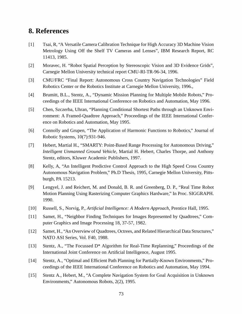
73

8. References

[1] Tsai, R, “A Versatile Camera Calibration Technique for High Accuracy 3D Machine VisionMetrology Using Off the Shelf TV Cameras and Lenses”, IBM Research Report, RC11413, 1985.

[2] Moravec, H. “Robot Spatial Perception by Stereoscopic Vision and 3D Evidence Grids”,Carnegie Mellon University technical report CMU-RI-TR-96-34, 1996.

[3] CMU/FRC “Final Report: Autonomous Cross Country Navigation Technologies” FieldRobotics Center or the Robotics Institute at Carnegie Mellon University, 1996.,

[4] Brumitt, B.L., Stentz, A., “Dynamic Mission Planning for Multiple Mobile Robots,” Pro-ceedings of the IEEE International Conference on Robotics and Automation, May 1996.

[5] Chen, Szczerba, Uhran, “Planning Conditional Shortest Paths through an Unknown Envi-ronment: A Framed-Quadtree Approach,” Proceedings of the IEEE International Confer-ence on Robotics and Automation, May 1995.

[6] Connolly and Grupen, “The Application of Harmonic Functions to Robotics,” Journal ofRobotic Systems, 10(7):931-946.

[7] Hebert, Martial H., “SMARTY: Point-Based Range Processing for Autonomous Driving,”Intelligent Unmanned Ground Vehicle, Martial H. Hebert, Charles Thorpe, and AnthonyStentz, editors, Kluwer Academic Publishers, 1997.

[8] Kelly, A, “An Intelligent Predictive Control Approach to the High Speed Cross CountryAutonomous Navigation Problem,” Ph.D Thesis, 1995, Carnegie Mellon University, Pitts-burgh, PA 15213.

[9] Lengyel, J. and Reichert, M. and Donald, B. R. and Greenberg, D. P., “Real Time RobotMotion Planning Using Rasterizing Computer Graphics Hardware,” In Proc. SIGGRAPH.1990.

[10] Russell, S., Norvig, P.,Artificial Intelligence: A Modern Approach, Prentice Hall, 1995.

[11] Samet, H., “Neighbor Finding Techniques for Images Represented by Quadtrees,” Com-puter Graphics and Image Processing 18, 37-57, 1982.

[12] Samet, H., “An Overview of Quadtrees, Octrees, and Related Hierarchical Data Structures,”NATO ASI Series, Vol. F40, 1988.

[13] Stentz, A., “The Focussed D* Algorithm for Real-Time Replanning,” Proceedings of theInternational Joint Conference on Artificial Intelligence, August 1995.

[14] Stentz, A., “Optimal and Efficient Path Planning for Partially-Known Environments,” Pro-ceedings of the IEEE International Conference on Robotics and Automation, May 1994.

[15] Stentz A., Hebert, M., “A Complete Navigation System for Goal Acquisition in UnknownEnvironments,” Autonomous Robots, 2(2), 1995.

74

[16] Stentz, A., “Best Information Planning for Unknown, Uncertain, and Changing Domains,”AAAI-97 Workshop on On-line-Search.

[17] Whitcomb, L. L. and Koditschek, D. E. “Automatic Assembly Planning and Control viaPotential Functions,” In Proc. IEEE/RSJ International Workshop on Intelligent Robots andSystems. 1991.

[18] Tsai, R, “A Versatile Camera Calibration Technique for High Accuracy 3D Machine VisionMetrology Using Off the Shelf TV Cameras and Lenses”, IBM Research Report, RC11413, 1985.

[19] Moravec, H. “Robot Spatial Perception by Stereoscopic Vision and 3D Evidence Grids”,Carnegie Mellon University technical report CMU-RI-TR-96-34, 1996.

[20] CMU/FRC “Final Report: Autonomous Cross Country Navigation Technologies” FieldRobotics Center or the Robotics Institute at Carnegie Mellon University, 1996.,