Embed Size (px)
Citation preview

Autonomous Bicycle Project
Team Final Report by:Sung Won An, Rannie Dong, Eric Huang, Jason Hwang,
Olav Imsdahl, Weier Mi, Arundathi Sharma, Rhett Wampler, Xiangyun (Joyce) Xu
Professor Andy RuinaBiorobotics and Locomotion Lab
Mechanical and Aerospace Engineering, Cornell University
Fall 2015

Abstract
We are developing a robotic bicycle that we hope can balance better than any previous
robotic two-wheeler (single-track vehicle). Many have tried using a variety of balance
strategies, including gyroscopes and reaction wheels. Our bicycle will use only steering
for balance, much like a human does. The mathematical model we use to develop
our controller uses a point-mass model of the bicycle and bicycle rider. We also use
simplified bicycle geometry with a vertical fork and no offset. The equations of such a
bike are more manageable than the non-linear equations of a full bicycle. The eventual
goal is to use massive computer optimization to find a steering strategy that maximizes
the disturbances from which the bike can right itself. In the meantime we will see how
well we can balance the bicycle using a steering angle rate (controlled by a motor) that
is a linear function of the instantaneous steer angle, the bike lean angle, and the bike
falling rate. When all put together, we hope to demonstrate the bike riding around
Cornell campus on its own.
i

Contents
Abstract i
Contents v
List of Figures vii
Acknowledgement viii
Nomenclature viii
1 Review of Other Robotic Bicycles 1
1.1 Introduction . . . . . . . . . . . . . . . . . . . . . . . . . . . . . . . . . . 1
1.2 Balance by Gyroscope . . . . . . . . . . . . . . . . . . . . . . . . . . . . 3
1.2.1 Bicycle Robot . . . . . . . . . . . . . . . . . . . . . . . . . . . . . 3
1.2.2 JyroBike . . . . . . . . . . . . . . . . . . . . . . . . . . . . . . . . 4
1.2.3 2012 BicyRobo Thailand Competition Runner-Up . . . . . . . . 5
1.2.4 Lit Motors . . . . . . . . . . . . . . . . . . . . . . . . . . . . . . 5
1.2.5 Why Don’t We Use Gyroscopes? . . . . . . . . . . . . . . . . . . 6
1.3 Balance by Reaction Wheel . . . . . . . . . . . . . . . . . . . . . . . . . 7
1.3.1 Auto Balanced Robotic Bicycle (ABRB) . . . . . . . . . . . . . . 7
1.3.2 One Track Vehicle . . . . . . . . . . . . . . . . . . . . . . . . . . 8
1.3.3 Why Don’t we Use Reaction Wheels . . . . . . . . . . . . . . . . 9
1.4 Balance by Steering . . . . . . . . . . . . . . . . . . . . . . . . . . . . . 9
1.4.1 RoboRealm Robotic Bicycle . . . . . . . . . . . . . . . . . . . . . 10
1.4.2 Micro Robot Bicycle . . . . . . . . . . . . . . . . . . . . . . . . . 10
1.4.3 RoboBiker . . . . . . . . . . . . . . . . . . . . . . . . . . . . . . . 11
1.4.4 Self Stabilizing Electric Bicycle . . . . . . . . . . . . . . . . . . . 11
1.4.5 Ghostrider . . . . . . . . . . . . . . . . . . . . . . . . . . . . . . 12
1.4.6 NXTBike-GS . . . . . . . . . . . . . . . . . . . . . . . . . . . . . 13
1.5 Goals . . . . . . . . . . . . . . . . . . . . . . . . . . . . . . . . . . . . . 13
2 Bicycle Dynamics and Development of a Controller for Stability and
ii

a State Observer 15
2.1 Dynamics: Deriving a Linearized Equation of Motion . . . . . . . . . . . 15
2.1.1 Point Mass Model . . . . . . . . . . . . . . . . . . . . . . . . . . 15
2.1.2 Deriving and Linearizing the Equation of Motion . . . . . . . . . 16
2.2 Developing a Controller . . . . . . . . . . . . . . . . . . . . . . . . . . . 17
2.2.1 Controller for Stability . . . . . . . . . . . . . . . . . . . . . . . . 18
2.2.2 Observer-based Controller for Reference Tracking . . . . . . . . . 20
2.3 References . . . . . . . . . . . . . . . . . . . . . . . . . . . . . . . . . . . 21
2.4 Binding and lettering . . . . . . . . . . . . . . . . . . . . . . . . . . . . . 21
2.5 Abstract . . . . . . . . . . . . . . . . . . . . . . . . . . . . . . . . . . . . 22
2.6 Paper . . . . . . . . . . . . . . . . . . . . . . . . . . . . . . . . . . . . . 22
2.7 Page numbers . . . . . . . . . . . . . . . . . . . . . . . . . . . . . . . . . 23
2.8 Footnotes . . . . . . . . . . . . . . . . . . . . . . . . . . . . . . . . . . . 23
2.9 Further advice . . . . . . . . . . . . . . . . . . . . . . . . . . . . . . . . 23
2.9.1 For Humanities and Social Sciences . . . . . . . . . . . . . . . . . 23
2.9.2 For Sciences, Engineering and Medicine . . . . . . . . . . . . . . 23
2.9.3 For all candidates . . . . . . . . . . . . . . . . . . . . . . . . . . 24
3 Inertial Measurement Unit 25
3.1 Background . . . . . . . . . . . . . . . . . . . . . . . . . . . . . . . . . . 25
3.1.1 Six Degrees of Freedom . . . . . . . . . . . . . . . . . . . . . . . 25
3.1.2 Euler Angles and Angular Rates . . . . . . . . . . . . . . . . . . 26
3.1.3 Drift . . . . . . . . . . . . . . . . . . . . . . . . . . . . . . . . . . 27
3.1.4 GyroBias Correction . . . . . . . . . . . . . . . . . . . . . . . . . 27
3.2 Code . . . . . . . . . . . . . . . . . . . . . . . . . . . . . . . . . . . . . . 27
3.2.1 Testing . . . . . . . . . . . . . . . . . . . . . . . . . . . . . . . . 27
3.2.2 BeagleBone Black Code . . . . . . . . . . . . . . . . . . . . . . . 27
3.2.3 IMU to PC . . . . . . . . . . . . . . . . . . . . . . . . . . . . . . 29
3.3 Results . . . . . . . . . . . . . . . . . . . . . . . . . . . . . . . . . . . . . 29
3.3.1 Without GyroBias . . . . . . . . . . . . . . . . . . . . . . . . . . 29
3.3.2 With GyroBias . . . . . . . . . . . . . . . . . . . . . . . . . . . . 35
3.3.3 Noise . . . . . . . . . . . . . . . . . . . . . . . . . . . . . . . . . 36
3.3.4 GyroBias Data . . . . . . . . . . . . . . . . . . . . . . . . . . . . 38
3.4 Implementation . . . . . . . . . . . . . . . . . . . . . . . . . . . . . . . . 42
3.4.1 Accessories . . . . . . . . . . . . . . . . . . . . . . . . . . . . . . 42
3.4.2 BeagleBone Black Setup . . . . . . . . . . . . . . . . . . . . . . . 43
3.4.3 Pre-run Procedures . . . . . . . . . . . . . . . . . . . . . . . . . . 45
4 Rotary Encoder 46
4.1 Overview . . . . . . . . . . . . . . . . . . . . . . . . . . . . . . . . . . . 46
iii

4.2 Basics . . . . . . . . . . . . . . . . . . . . . . . . . . . . . . . . . . . . . 47
4.3 Working Mechanism . . . . . . . . . . . . . . . . . . . . . . . . . . . . . 48
4.3.1 Opti-laser based Incremental Encoders . . . . . . . . . . . . . . . 48
4.3.2 Magnetic based Incremental Encoders . . . . . . . . . . . . . . . 48
4.4 Encoder Properties . . . . . . . . . . . . . . . . . . . . . . . . . . . . . . 49
4.5 Encoder Outputs . . . . . . . . . . . . . . . . . . . . . . . . . . . . . . . 51
4.5.1 Quadrature Output . . . . . . . . . . . . . . . . . . . . . . . . . 51
4.5.2 Counting on the edges . . . . . . . . . . . . . . . . . . . . . . . . 51
4.6 Angular Speed Calculation . . . . . . . . . . . . . . . . . . . . . . . . . 52
4.7 Encoder Functionality Test . . . . . . . . . . . . . . . . . . . . . . . . . 53
4.8 Encoder Circuit . . . . . . . . . . . . . . . . . . . . . . . . . . . . . . . . 54
4.8.1 Differential Line Receiver . . . . . . . . . . . . . . . . . . . . . . 54
4.8.2 Opto-isolator . . . . . . . . . . . . . . . . . . . . . . . . . . . . . 54
4.9 Connection to the Beaglebone Black . . . . . . . . . . . . . . . . . . . . 56
4.10 Alternatives . . . . . . . . . . . . . . . . . . . . . . . . . . . . . . . . . . 56
4.10.1 Potentiometer . . . . . . . . . . . . . . . . . . . . . . . . . . . . . 56
4.10.2 Encoder vs Potentiometer . . . . . . . . . . . . . . . . . . . . . . 57
5 Code 59
5.1 Overview . . . . . . . . . . . . . . . . . . . . . . . . . . . . . . . . . . . 59
5.2 Control Code . . . . . . . . . . . . . . . . . . . . . . . . . . . . . . . . . 60
5.3 System Code . . . . . . . . . . . . . . . . . . . . . . . . . . . . . . . . . 62
5.3.1 eQEP driver . . . . . . . . . . . . . . . . . . . . . . . . . . . . . 62
5.3.2 UART Interface . . . . . . . . . . . . . . . . . . . . . . . . . . . 64
5.3.3 ADAfruit BBIO . . . . . . . . . . . . . . . . . . . . . . . . . . . 64
6 Front steering and Mechanical Design 66
6.1 Overview . . . . . . . . . . . . . . . . . . . . . . . . . . . . . . . . . . . 66
6.2 Front Steering . . . . . . . . . . . . . . . . . . . . . . . . . . . . . . . . . 67
6.2.1 Fork Insert . . . . . . . . . . . . . . . . . . . . . . . . . . . . . . 68
6.2.2 Orthogonal plate . . . . . . . . . . . . . . . . . . . . . . . . . . . 69
6.2.3 Coupling . . . . . . . . . . . . . . . . . . . . . . . . . . . . . . . 70
6.2.4 Encoder on the back . . . . . . . . . . . . . . . . . . . . . . . . . 71
6.3 Inertial Measurement Unit mount . . . . . . . . . . . . . . . . . . . . . . 72
6.4 Foldable starting and landing gear . . . . . . . . . . . . . . . . . . . . . 73
7 Printed Circuit Board Design 76
7.1 Overview . . . . . . . . . . . . . . . . . . . . . . . . . . . . . . . . . . . 76
7.1.1 Printed Circuit Board . . . . . . . . . . . . . . . . . . . . . . . . 76
7.1.2 Through-hole versus Surface-mounting . . . . . . . . . . . . . . . 77
iv

7.2 Design Software . . . . . . . . . . . . . . . . . . . . . . . . . . . . . . . . 78
7.2.1 Introduction . . . . . . . . . . . . . . . . . . . . . . . . . . . . . 78
7.2.2 Project . . . . . . . . . . . . . . . . . . . . . . . . . . . . . . . . 79
7.2.3 Schematic . . . . . . . . . . . . . . . . . . . . . . . . . . . . . . . 79
7.2.4 Board . . . . . . . . . . . . . . . . . . . . . . . . . . . . . . . . . 80
7.2.5 Library . . . . . . . . . . . . . . . . . . . . . . . . . . . . . . . . 81
7.3 Printed Circuit Board Components . . . . . . . . . . . . . . . . . . . . . 84
7.3.1 Delta DC/DC Converter . . . . . . . . . . . . . . . . . . . . . . . 84
7.3.2 Opto-isolator . . . . . . . . . . . . . . . . . . . . . . . . . . . . . 84
7.3.3 Differential Line Receiver . . . . . . . . . . . . . . . . . . . . . . 87
7.3.4 Operational Amplifier (Op-amp) . . . . . . . . . . . . . . . . . . 88
7.3.5 Connectors . . . . . . . . . . . . . . . . . . . . . . . . . . . . . . 88
7.4 Major Adjustments from Our Previous Design . . . . . . . . . . . . . . . 90
7.4.1 Pololu Motor Controller . . . . . . . . . . . . . . . . . . . . . . . 90
7.4.2 Decoupling Capacitors . . . . . . . . . . . . . . . . . . . . . . . . 91
A Example Appendix 92
Bibliography 93
Index 93
v

List of Figures
1.1 Two-wheeled self-balancing automobile concept described in 2 Boys in a
GyroCar.1 . . . . . . . . . . . . . . . . . . . . . . . . . . . . . . . . . . . 2
1.2 The Shilosky Gyrocar.2 . . . . . . . . . . . . . . . . . . . . . . . . . . . 2
1.3 Bicycle Robot.3 . . . . . . . . . . . . . . . . . . . . . . . . . . . . . . . . 4
1.4 JyroBike.4 . . . . . . . . . . . . . . . . . . . . . . . . . . . . . . . . . . . 5
1.5 C-1 electric motorcycle by Lit Motors.5 . . . . . . . . . . . . . . . . . . 6
1.6 ABRB completed design.6 . . . . . . . . . . . . . . . . . . . . . . . . . . 8
1.7 ABRB schematic design.7 . . . . . . . . . . . . . . . . . . . . . . . . . . 8
1.8 One Track Vehicle.8 . . . . . . . . . . . . . . . . . . . . . . . . . . . . . 9
1.9 RoboRealm Robotic Bicycle.9 . . . . . . . . . . . . . . . . . . . . . . . . 10
1.10 RoboBiker.10 . . . . . . . . . . . . . . . . . . . . . . . . . . . . . . . . . 11
1.11 Self Stabilizing Electric Bicycle.11 . . . . . . . . . . . . . . . . . . . . . . 12
1.12 Ghostrider.12 . . . . . . . . . . . . . . . . . . . . . . . . . . . . . . . . . 12
1.13 NXTBike-GS (Legos).13 . . . . . . . . . . . . . . . . . . . . . . . . . . . 13
26
3.2 Flat-Roll-Flat:Fast . . . . . . . . . . . . . . . . . . . . . . . . . . . . . . 30
3.3 Flat-Roll-Flat:Medium . . . . . . . . . . . . . . . . . . . . . . . . . . . . 31
3.4 Flat-Roll-Flat:Slow . . . . . . . . . . . . . . . . . . . . . . . . . . . . . . 31
3.5 Rotated about Yaw - Fast . . . . . . . . . . . . . . . . . . . . . . . . . . 33
3.6 Rotated about Yaw - Medium . . . . . . . . . . . . . . . . . . . . . . . . 33
3.7 Rotated about Yaw - Slow . . . . . . . . . . . . . . . . . . . . . . . . . . 34
3.8 Yaw vs Roll with Correction . . . . . . . . . . . . . . . . . . . . . . . . . 35
3.9 Initial Angles when Flat . . . . . . . . . . . . . . . . . . . . . . . . . . . 37
3.10 Flat for 30 Minutes . . . . . . . . . . . . . . . . . . . . . . . . . . . . . . 38
47
50
50
51
55
57
vi
6.1 front steering overview . . . . . . . . . . . . . . . . . . . . . . . . . . . . 67
6.2 front wheel with fork insert and coupling . . . . . . . . . . . . . . . . . . 68
6.3 plate connected to steel on the bottom and holding the 4 long rods . . . 69
6.4 the coupling between the motor (top) and the encoder (bottom) . . . . 70
6.5 the encoder (black box) sits on the end of the motor . . . . . . . . . . . 71
6.6 the IMU mount is clamped to the bike frame (blue) . . . . . . . . . . . 72
6.7 wheels, gear and motor connected to bike . . . . . . . . . . . . . . . . . 73
6.8 reverse side with end-stops . . . . . . . . . . . . . . . . . . . . . . . . . . 74
6.9 circuit with end-stops . . . . . . . . . . . . . . . . . . . . . . . . . . . . 75
7.1 Printed Circuit Board.14 . . . . . . . . . . . . . . . . . . . . . . . . . . . 77
7.2 Breadboard.15 . . . . . . . . . . . . . . . . . . . . . . . . . . . . . . . . . 77
7.3 Through-hole resistor.16 . . . . . . . . . . . . . . . . . . . . . . . . . . . 78
7.4 Surface-mount capacitor.17 . . . . . . . . . . . . . . . . . . . . . . . . . 78
7.5 The Project Interface. . . . . . . . . . . . . . . . . . . . . . . . . . . . . 79
7.6 The Schematic Interface. . . . . . . . . . . . . . . . . . . . . . . . . . . . 80
7.7 The Board Interface. . . . . . . . . . . . . . . . . . . . . . . . . . . . . . 81
7.8 The Library Interface. . . . . . . . . . . . . . . . . . . . . . . . . . . . . 82
7.9 A built package of Pololu Motor Controller. . . . . . . . . . . . . . . . . 83
7.10 A built Symbol of Pololu Motor Controller. . . . . . . . . . . . . . . . . 83
7.11 A built Device and pin connections of Pololu Motor Controller. . . . . . 83
7.12 The overall schematic. . . . . . . . . . . . . . . . . . . . . . . . . . . . . 85
7.13 Delta DC/DC Converter in the Schematics. . . . . . . . . . . . . . . . . 86
7.14 An opto-isolator in the Schematics. . . . . . . . . . . . . . . . . . . . . . 87
7.15 Line-receiver in the Schematics. . . . . . . . . . . . . . . . . . . . . . . . 88
7.16 Op-amp circuit in the Schematics. . . . . . . . . . . . . . . . . . . . . . 89
7.17 The connector that’s supposed to connect to the Beaglebone Black in
the Schematics. . . . . . . . . . . . . . . . . . . . . . . . . . . . . . . . . 90
vii

Acknowledgement
The author wishes to thank the University of Liverpool Computing Services Department
for the development of this LATEX thesis template.
viii

Chapter 1
Review of Other RoboticBicycles
Contributor: Sung Won An
1.1 Introduction
The concept of self-balancing two-wheeled vehicles dates back to 1911, in a work of
fiction by Kenneth Brown titled, "Two Boys in a GyroCar", as shown in Fig.1.1. Since
then, there have been numerous attempts to build a self-stabilizing two-wheeled vehicle.
In 1912, Pyotr Shilovsky, a member of the Russian royal family, commissioned the
Shilovski Gyrocar. The Wolseley Tool and Motorcar Company manufactured the design
in Fig.1.2 in 1914, which weighed 2.75 tons and had a large turning radius. Since the
20th century, we have come much closer to realizing this goal. Today, there are a large
variety of self-stabilizing bicycles and motorcycles that have been explored. These
vehicles range from commercial bicycles that are available on the market to simple
concepts that have never been built.
1

Figure 1.1: Two-wheeled self-balancing automobile concept described in 2 Boys in aGyroCar.1
All self-stabilizing two-wheeled vehicles can be grouped into three categories based on
the specific method by which the vehicle achieves balance. These categories are: balance
by gyroscope, balance by reaction wheel, and balance by steering. Many advances have
already been made towards building highly stable vehicles that balance by gyroscope
or by a reaction wheel. However, in the context of human interaction with a bicycle
or motorcycle, gyroscopes and reaction wheels tend to be irrelevant. Our research
group is interested in studying balance by steering to gain a better understanding the
mechanisms by which we balance on bicycles. In this final category, the problem yet
remains in building a sufficiently stable bicycle.
Figure 1.2: The Shilosky Gyrocar.2
1Kenneth Brown. Two Boys in a GyroCar. Digital image. Amazon. Web. 30 October 2015.
2

1.2 Balance by Gyroscope
The gyroscope category consists of vehicles that use a massive wheel that spins at
high speeds in order to keep stable. This method exploits gyroscopic effects and the
conservation of angular momentum. In simpler terms, a massive spinning object, in
an effort to maintain its angular momentum, will provide forces opposing those which
make the bicycle unstable. As long as the object has enough mass and rotates at a high
enough speed, the forces are enough to prevent tipping over. Within this category, two
different orientations are most common. Recall that the angular momentum vector of a
spinning object is parallel to the axis about which it spins. In Fig. ??, a spinning top has
its angular momentum vector either pointing straight up or straight down, depending
on if it spins clockwise or counterclockwise. Additionally, a spinning wheel, shown in
Fig. ??, of a bicycle has its angular momentum vector pointing perpendicularly out
from the bicycle. The spinning top and wheel orientations are most common for the
gyroscope. As one can see, in order for the gyroscope to be effective, the angular
momentum vector must be perpendicular to the direction of motion. In the following
sections, we will give an overview of each gyroscopic bicycle that we have been able to
find in existence.
1.2.1 Bicycle Robot
Shown in Fig. 1.3, this bicycle uses a large gyroscope in a top orientation attached above
the rear wheel to balance. It was built by Bui Trung Thanh at the Asian Institute of
Technology. It is remote controlled and can balance while motionless, as well as in
motion. There are motors on the front wheel to control steering direction and the back
wheel to drive the bicycle. The robot was programmed using C on the ATMEGA128
micro-controller.
2Pyotr Shilovsky. Shilovski Gyrocar. Digital image. Wikipedia. Web. 30 October 2015.
3

Figure 1.3: Bicycle Robot.3
1.2.2 JyroBike
The JyroBike is one of the only commercially-available self-stabilizing bicycles. The
bicycle is shown in Fig. 1.4. It balances by using a flywheel, which is simply a gyro-
scope in its wheel orientation. The flywheel is placed inside the front wheel and spins
separately from the wheel itself. The JyroBike product is available as both the entire
bicycle or the standalone front wheel with the flywheel. As a commercial product, it
includes many features not found in other gyroscopic bicycles, such as a power button,
flywheel speed control, and a rechargeable battery.
3Bui Trung Thanh. Bicycle Robot. Digital image. Youtube. Web. 30 October 2015.
4

Figure 1.4: JyroBike.4
1.2.3 2012 BicyRobo Thailand Competition Runner-Up
A team from King Mongkut’s University of Technology created a self-balancing robotic
bicycle using gyroscopes. This bicycle was created to compete in the 2012 BicyRobo
Thailand Competition, which is a competition for self-stabilizing bicycles hosted by the
Asian Institute of Technology in Thailand. It uses two gyroscopes in the top orientation,
one on either side of the bicycle. As the bicycle tips to one side, the platforms that
the gyroscopes are placed on tip forwards and backwards to balance the bicycle. This
entails the use of sensors to detect tilt, such as an IMU or an accelerometer.
1.2.4 Lit Motors
Lit Motors is another company that seeks to commercially market their self-stabilizing
vehicle. Their main product, the C-1, is a fully electric two-wheeled self-balancing
motorcycle. As you can see in Fig. 1.7, the vehicle has doors, headlights, brake lights,
and windows like a car, but has only two wheels. The C-1 is still in development,
but some basic information about its design is available online. It balances using two
4JyroBike LTD. JyroBike. Digital image. KickStarter. Web. 30 October 2015.
5

gyroscopes and is powered by lithium iron phosphate batteries. The gyroscopes enable
the motorcycle to lean in and out of turns, as a non-stabilizing motorcycle would. It
weighs 800 lbs and can ride up to 200 miles on one charge. By comparison, most electric
motorcycles weigh downwards of 500 lbs and can ride up to similar distances on a single
charge.
Figure 1.5: C-1 electric motorcycle by Lit Motors.5
1.2.5 Why Don’t We Use Gyroscopes?
Although gyroscopes are highly stable, the use of a gyroscope requires a very compli-
cated design with high weight and cost. This is because the wheel needs to be massive
enough and needs to be spinning continuously in order for the bicycle to remain stable.
This entails an incredible drain in energy and is not sustainable. As mentioned above,
the weight ratio between the C-1 electric balancing motorcycle and regular electric mo-
torcycles is close to 1.6. Additionally, a gyroscope often resists turns as a consequence
of its high stability. Riding a gyroscopic bicycle is analogous to riding a tricycle. A tri-
cycle, as we all know, provides stability to a bicycle with the addition of training wheels
on either side. However, this provides too much stability since the rider is unable to
lean into a turn as he or she would on a regular bicycle. The two training wheels pre-
vent any tilt in the bicycles motion; to turn, the rider is forced to lean in the opposite
direction. Gyroscopic bicycles are similar in that they are counterproductive in both
teaching how to ride a bicycle and learning how humans balance on bicycles.
5Lit Motors. C-1 Electric Motorcycle. Digital image. Lit Motors. Web. 30 October 2015.
6

1.3 Balance by Reaction Wheel
The reaction wheel category consists of bicycles that again use a massive wheel with
a high moment of inertia. However, instead of having a continuously spinning wheel,
the reaction wheel only spins when necessary, to provide sufficient torque to counteract
gravity and keep the bicycle from falling. This is also possible through the conservation
of angular momentum; as the reaction wheel spins in one direction, it applies a torque
on the bicycle in the opposite direction. Since the amount of torque is proportional to
how fast the reaction wheel spins, it can be calculated very precisely to keep the bicycle
very stable. The reaction wheel also differs from a gyroscope in that it is generally
placed perpendicular to the axis of the bike and the ground, similar to the orientation
of a steering wheel. Of the reaction-wheel-balanced bicycles found in research, none
exhibited the ability to turn. Most either follow a straight path or only stay upright.
Although the reaction wheel is also a very stable method, it is not suitable for our
purposes, as shown in the following sections.
1.3.1 Auto Balanced Robotic Bicycle (ABRB)
Students at George Mason University built a two-inline-wheel robot capable of self-
balancing using a reaction wheel. See Fig. ?? for a detailed schematic and Fig. ??
for the completed product. The design is fairly simple: a low-riding scooter with fixed
wheels. The wheels were 12-inch bicycle wheels and the reaction wheel was placed
roughly in the middle of the robot with a diameter of 8 inches. In order to attain a
high moment of inertia while limiting the overall mass, the reaction wheel was custom
machined out of steel to have its mass concentrated on the outer edge. The ABRB has
been tested to perform well when driving forwards, backwards, and stopping. It also
performed well under conditions when small disturbances were introduced.
The ABRB balancing system used a Motorola M68HC11 microcontroller and two sen-
sors to read tilt angle: the ADIS16209 inclinometer and the ADXRS401 gyroscope. The
redundancy in these devices was used to correct for gyrscopic drift. The ABRB drive
system used two different microcontrollers: the AVR ATmega32 from Atmel and an
AVR ATtiny25 also from Atmel. The first was used for the more complex drive control
logic and the latter was used to receive signals from a hand-held remote control. The
drive motor used was a Pittman 8712 brushed DC motor.
7

Figure 1.6: ABRB completed design.6
Figure 1.7: ABRB schematic design.7
1.3.2 One Track Vehicle
A researcher by the name of Gunnar Schmidt created a similar robot at the Technical
University of Berlin. He started his design incrementally by first building a robot to
balance an inverted pendulum with small disturbances using the CHR-6DOF IMU to
detect tilt angles. The final reaction wheel used was a 12 inch bicycle wheel with metal
plates around its edge to give it a larger moment of inertia. Unlike above, this bicycle
was only tested to maintain balance while motionless. The final specifications were 25.2
kg for the bicycle with 7.4 kg attributed to the reaction wheel. The motor used was
a Faulhaber DC motor. This bicycle was less of a success than that of above, since it
was seen to exhibit oscillations under certain condiditons, which can be attributed to
flaws in the controller feedback loop. The bicycle can be found below in Fig. ??.
6George Mason University. Auto Balanced Robotic Bicycle. Digital image. George Mason Univer-sity. Web. 30 October 2015.
7George Mason University. Auto Balanced Robotic Bicycle. Digital image. George Mason Univer-sity. Web. 30 October 2015.
8

Figure 1.8: One Track Vehicle.8
1.3.3 Why Don’t we Use Reaction Wheels
Reaction wheels exhibit the same major flaw as gyroscopes: they must be heavy enough!
This limits the weight for other components on the vehicle since a bicycle is largely
thought to be light enough to carry, if needed. Additionally, both bicycles shown
above have no means of turning. That is not to say that turning would be impossible
to accomplish with a reaction-wheel-balanced bicycle, it just has not been done yet.
Additionally, imagine how difficult it would be to ride a bicycle that would jerk upright
every time it began to tilt. For the interest of studying human balance on bicycles and
the goal of completing a safer, ride-able, learning bicycle, the reaction wheel design
entails many characteristics that are ultimately unhelpful.
1.4 Balance by Steering
The last category is the one our team is interested in: balance by steering. This category
consists of bicycles that simply steer to correct tilt angle and keep the bicycle stable.
This method is most akin to how humans generally ride bicycles and is most suitable
for our goals. The method itself does not entail many design constraints other than an
extra motor to control steering, which is akin to the extra motor for the two categories
8Gunnar Schmidt. One Track Vehicle. Digital image. Technical University of Berlin. Web. 30October 2015.
9

previously. However, with balance by steering unlike the previous category, there is
no longer the weight constraint. Despite this apparent advantage, a common trend
appeared amongst bicycles that use steering to balance. Bicycles that used steering
for balance were either highly unstable or were only stable at moderately high speeds.
These bicycles were seen to be very wobbly, even when undisturbed.
1.4.1 RoboRealm Robotic Bicycle
The Science and Technology Research Institute (STRI) Robotics Team built an auto-
balanced, auto-steering, ride-able robotic bicycle, shown in Fig. 1.9 to enter in the
BicycRobo Thailand Competition in 2010. The bicycle can only balance while moving
at moderately high speeds and is can be controlled either remotely or via image process-
ing. It uses a combination of encoders, potentiometers, gyroscopes, and accelerometers
for sensor data, as well as a webcam for image processing. It is only moderately stable,
as it experiences slight jitters due to either over or under-compensation by the steering
wheel.
Figure 1.9: RoboRealm Robotic Bicycle.9
1.4.2 Micro Robot Bicycle
The Micro Robot Team from the Mahanakorn University of Technology built a bicycle
similar to the one above that balances by steering for the same competition. It uses a
compass for navigation as well as some form of image processing. This bike, similar to
the one above, also seems to have trouble riding in a straight line without veering off
course. Additionally, it is unable to maintain stability at zero speed.
9STRI Robot Team. RoboRealm. Digital image. Science and Technology Research Institute. Web.30 October 2015.
10
1.4.3 RoboBiker
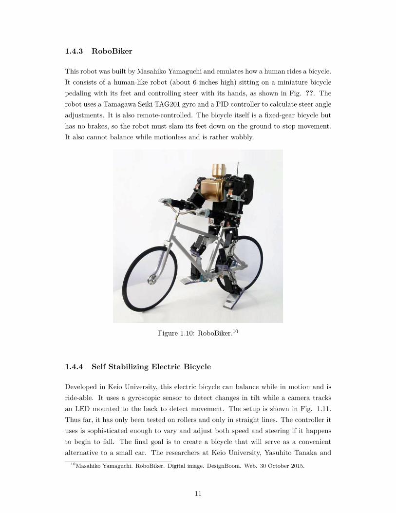
This robot was built by Masahiko Yamaguchi and emulates how a human rides a bicycle.
It consists of a human-like robot (about 6 inches high) sitting on a miniature bicycle
pedaling with its feet and controlling steer with its hands, as shown in Fig. ??. The
robot uses a Tamagawa Seiki TAG201 gyro and a PID controller to calculate steer angle
adjustments. It is also remote-controlled. The bicycle itself is a fixed-gear bicycle but
has no brakes, so the robot must slam its feet down on the ground to stop movement.
It also cannot balance while motionless and is rather wobbly.
Figure 1.10: RoboBiker.10
1.4.4 Self Stabilizing Electric Bicycle
Developed in Keio University, this electric bicycle can balance while in motion and is
ride-able. It uses a gyroscopic sensor to detect changes in tilt while a camera tracks
an LED mounted to the back to detect movement. The setup is shown in Fig. 1.11.
Thus far, it has only been tested on rollers and only in straight lines. The controller it
uses is sophisticated enough to vary and adjust both speed and steering if it happens
to begin to fall. The final goal is to create a bicycle that will serve as a convenient
alternative to a small car. The researchers at Keio University, Yasuhito Tanaka and
10Masahiko Yamaguchi. RoboBiker. Digital image. DesignBoom. Web. 30 October 2015.
11

Tohsiyuki Murakami, aim to be able to stabilize the bicycle at zero speed, implying
that it does not yet exhibit the ability to do that.
Figure 1.11: Self Stabilizing Electric Bicycle.11
1.4.5 Ghostrider
Shown in Fig. 1.12, the Ghostrider was built to enter in the DARPA Grand Challenge
by a team at the University of California, Berkeley. In building the robotic motorcycle,
the team also built a custom Inertial Angle Sensor, capable of 100KHz baud rate
and 0.02 degrees resolution. Despite this custom sensor, the motorcycle itself is very
wobbly and cannot balance while motionless. It uses both GPS and image processing
to navigate past obstacles.
Figure 1.12: Ghostrider.12
11Keio University. Self Stabilizing Electric Bicycle. Digital image. Phys.org. Web. 30 October 2015.
12

1.4.6 NXTBike-GS
Built at the Delft University of Technology, this robot, as seen in Fig. 1.13, was built
out of Lego pieces and programmed using a Lego Mindstorms NXT. The robot also uses
a rotary encoder for steering the front wheel and a Hitechnics Gyro Sensor to detect
tilt. Another DC motor was used to drive the back wheel. Although the robot is small,
it still exhibits some wobble in its path. Unlike its less successful counterparts, it is able
to turn and balance while turning, though it cannot balance while motionless.
Figure 1.13: NXTBike-GS (Legos).13
1.5 Goals
As shown in the preceding sections, a steering bicycle with the ability to balance while
motionless has yet to be built. Even amongst the bicycles/motorcycles already built
that use balance by steering, none exhibit high stability and high recoverability. Our
goals include building an autonomous bicycle that falls in the third category that not
12University of California at Berkeley. Ghostrider. Digital image. WeMakeMoneyNotArts. Web. 30October 2015.
13Delft University of Technology. NXTBike-GS. Digital image. Mathworks. Web. 30 October 2015.
13

only is highly stable at low/zero speeds but can also easily recover from external distur-
bances. We also aim to have the bicycle navigationally autonomous, by using GPS and
image processing. Very few existing bikes were found to have the ability to navigate
autonomously and those that did, were not meant to leave a pre-designated track with
clear lanes.
14

Chapter 2
Bicycle Dynamics andDevelopment of a Controller forStability and a State Observer
Contributors: Arundathi Sharma
This chapter is a synthesis of the Autonomous Bicycle Project’s Fall 2014 and Spring
2015 Dynamics and Controls Paper, by Shihao Wang, Joong Gon Yim, Alex Abrams,
and Binghan He
In this section, we present the mathematical model of the bicycle that we are using and
derive the equations of motion for such a bicycle. We also review the derivation of a
stabilizing controller that should keep the bicycle upright, and the development of an
observer, which will estimate the state of the bicycle.
2.1 Dynamics: Deriving a Linearized Equation of Mo-tion
2.1.1 Point Mass Model
[INCLUDE PICTURE OF DIAGRAM WITH LABELED ANGLES]
From the figure above, we define geometry as follows:
G = center of mass
AD =front fork
BG=b
l = wheelbase AB
φ = lean angle
ψ = yaw angle (heading)
15

δ = steer angle
α = angle between front wheel and CD
xG = x-position of the center of mass
yG = y-position of the center of mass
zG = z-position of the center of mass
v = forward velocity of bicycle (assumed constant)
C = the contact point between the rear wheel and ground
D = the contact point between the front wheel and ground
2.1.2 Deriving and Linearizing the Equation of Motion
We use the physical model of the bicycle outlined above to find an equation describing
the motion of the bicycle’s center of mass. Refer to Shihao Wang’s Fall 2014 report in
the appendix for a detailed kinematic derivation. The resultant equation is:
(2.1)~aG = (v − h cos (φ) ˙(φ)ψ − h sin (φ)ψ − h cos (φ)φψ − bφ2)λ+
+(bψ − h sin (φ)φ+ vψ − h sin (φ)ψ2)n− (h cos (φ)φ2 + h sin (φ)φ)k
where λ runs parallel to the bicycle’s direction of motion, n is normal to λ in the ground
plane, and k points opposite to earth’s gravity.
This equation is useful, but we want to use this equation to control a bicycle. What
parameters are out of our control? We cannot control ψ, ψ, and α. Note: α is distinct
from δ because for a given steer angle, the angle α changes as the bicycle leans.
Again, see the appendix for a fully detailed derivation, the results of which are:
ψ =v tanα
l
and
tanα =tan δ
cosφ
Putting these two expressions together, and then taking a derivative to obtain ψ, we
can substitute into the original equation to describe the acceleration of the bicycle’s
center of mass using only lean and steer angle terms. We can measure lean and steer
angles, and can control steer angle, so this equation is what we want.
Now, we use our information about the motion of the center of mass to obtain a
differential equation. (See appendix for full derivation). This is done by performing
16

an angular momentum balance about point C (rear wheel contact point with ground).
Taking forward velocity v to be constant, we obtain an equation that contains the
most important parameters: lean angle, angular velocity, and acceleration, and steer
angle and angular velocity. Since we want to work with a first-order linear differential
equation, we linearize the equation that we just found by using standard small-angle
approximations for sin θ, tan θ, and cos θ. Although the bicycle is a nonlinear system
(which we see in our non-linear equation of motion), we approximate its motion in a
small region about the desired equilibrium point (φ = 0, for straight riding) as linear.
Note that if we deviate too much from a particular small region about equilibrium,
our controller may not be able to recover from a perturbation because the bicycle’s
behavior will no longer be linear. Eventually, (see appendix for algebra) we obtain a
linearized expression that looks like:
v2δ + bvδ = hlφ− glφ
. Rearranging for the relevant term:
φ =g
hφ−
v2
hlδ −
bv
hlδ
2.2 Developing a Controller
From the above differential form, we can put our equation into state space form, which
is a useful form for developing a controller. It looks like:
φ
φ
δ
=
0 1 0gh
0 −v2
hl
0 0 0
φ
φδ
+
0
−bvhl
1
δ
Observe that if we evaluate the right-hand side of the above equation, we will obtain
a set of three differential equations that apply to our system. We call x =
φ
φδ
our
state, which fully defines our system, the bicycle. If we know these three parameters,
we have fully defined the state of the bicycle at a moment in time. In a general sense,
the equation above is the same as:
x = Ax+Bu,
where the matrices A and B are properties of our system. A describes the extent to
which the state of the system is affected by itself i.e., how do the values of φ, φ, δ at a
point in time affect how those values change in time (φ, φ, δ). You might also call this
17

the natural behavior of the system. The eigenvalues of A would give us the solution
to the differential equations that we used to produce this state space equation. B
describes the extent to which our control input signal, u = −Kx (δ for the bicycle),
affects the state. We want to develop a controller, represented by a matrix K, such
that the above generalized equation can be rewritten as:
x = (A−BK)x,
We also define an output y = Cx, which represents our control variable:
y =[
1 0 0]
φ
φδ
As you can see, it outputs a value φ. Ideally, we want our input and output to eventu-
ally be equal values.
To design the controller, we need to consider some Ades, which represents the de-
sired behavior of the system, as it is affected by its own, controlled state (analogous to
A in x = Ax + Bu. Just as the eigenvalues of matrix A would describe the solutions
to the differential equation that we used to derive the original behavior of the system,
the eigenvalues of Ades represent the solutions to the differential equation describing
our desired behavior. So we use this fact to solve for a suitable K.
2.2.1 Controller for Stability
We find K according to our design requirements for the controlled behavior of the
bicycle. In our case, we want the bicycle to stabilize itself in a short amount of time,
say under 0.1s. We also want to prevent the bicycle from oscillating about φ = 0 at
high frequency. To do this, we assign a desired overshoot to our control response to be
less than 5%. <-CHECK THIS
We can employ a number of different methods to actually develop a controller that
meets these requirements. You can see what these methods are and how they were
employed to obtain a controller in the appendix section. The important thing is that
we went on to develop such a controller for a point-mass bicycle stabilization:
K =[
−843.1298 −119.7419 8.2379]
When this was put into a basic MATLAB simulation, these were the plots we obtained,
to describe the behavior of the bicycle.
18

[INSERT PICTURES OF PLOTS FROM SHIHAO’S REPORT]
Based on these plots, the theoretical bicycle stabilizes within the desired time frame
from a initial displacement lean angle φ = π4. Furthermore, the bicycle trajectory be-
haves as we expect it to for this situation, so this controller can, at least in theory,
successfully balance a bicycle modeled as a point-mass.
What of the actual bicycle? The controller above was derived using guessed values
for certain parts of the bicycle geometry. But since we are trying to develop a con-
troller for our own bicycle, we can customize. We can pretend the real bicycle is a
point-mass by finding its center of mass, and then plugging in relevant parameters in
order to find a controller that will work specifically for our bicycle. Quoting the Spring
2015 Controls report:
"In order to design a controller for the bicycle, we should know the value of the ge-
ometric parameters of the real bicycle. Mass doesn’t appear in the A or B matrices,
and g is a constant. Therefore, we only need to measure the position of the center of
mass (COM) relative to the rear wheel contact point C. We can find the center of mass
of an irregular object quite easily. If we let it hang freely, the center of mass is directly
below where we hang it from. If we then hang the object from a couple of other points and
draw the lines that go vertically downwards, the center of mass is where the lines meet."
INSERT PICTURE OF BICYCLE
Here are the parameters that were measured off the real bicycle:
• l = 0.9144m, wheel base distance
• b = 0.331m, horizontal distance between COM and rear wheel contact point
• d = 0.5834
• h = 0.3445m, height of COM
• v = 3.57m/s, forward speed
• g = 9.81 ms2 , gravity constant
Now, using these values for the real bicycle and implementing them in the same way as
we did before, we obtain a new, perhaps more applicable controller than the one where
we assumed arbitrary values for those numbers:
K =[
−3.4215 −0.8439 4.3345]
With an initial lean of π/6, this controller also appears to stabilize a bicycle in a simple
MATLAB ode45 simulation:
19

INSERT PLOTS
The three big problems that we could encounter with this controller are:
• Since the real bicycle is a nonlinear system, the nonlinear terms in the equation of
motion will dominate its motion when our linearization approximation becomes
invalid outside a certain range
• The controller may or may not be able to account for inaccuracies in the measured
or calculated parameters for the bicycle
• The method used to construct this controller is subjective (see: pole placement
method)
• Our control variable is δ. Ideally, we want to make the most out of the output
torque from our steering motor, so we should design our controller such that
the maximum steer angular velocity required to turn the handlebars at any time
would be 400rpm (the rating for our 24V 80W Maxon F 2260 motor).
So, we can work off our initial controller to optimize it further and ensure it is robust
enough to balance our bicycle. This is done by an algorithm called Linear-quadratic
Regulator (LQR), which is a more systematic way of finding a controller. This makes
it suitable for automation. MATLAB has a command that performs this optimization,
and gives us the following:
K =[
−38.3748 −4.1949 9.5922]
Again, we perform a simulation, and from an initial lean angle φ = π3
and obtain the
following plots, showing that the bike stabilizes:
INSERT PLOTS
2.2.2 Observer-based Controller for Reference Tracking
We developed the controller in the previous subsection under the assumption that we
knew all the state variables. However, in real life, that may not be the case. So, we
create an observer-based controller. A state observer will estimate our state variables
based on measurements that we make of the control variable (lean angle, in our case)
and other output variables. The observer has the same mathematical form as the
system itself, because it is trying to estimate the state. Meanwhile, the controller is
trying to achieve the desired state (whatever that may be–it may be different from
φ = 0 in case we have a different reference trajectory, e.g., when the bicycle is turning).
The observer looks like:
˙x = AΛx+Bu+H(y − CΛx),
20

where u = −KΛx, Λx is our estimate of the state, y is the output, and x is the actual state.
We are interested in the accuracy of our estimate, so we define an error, e = x− x, so
that our equation above can be more usefully expressed as:
e = (A−HC)e
Just as we previously wanted some matrix Ades such that the bicycle would behave a
certain way, we want to find A − HC such that the observer behaves a certain way;
specifically, we want our error, e, to become zero as quickly as possible. Again, we
can find a matrix H that makes this possible, just as we found K previously. The
methods for doing this are very similar to those used to find the stability controller,
and are detailed in the appendix. What we ultimately come up with is a value for H
as follows:
H =
782028
−11137
Putting the assembled controller with observer, we hope to see how our controller’s
step response. In MATLAB, this is what we see:
INCLUDE PLOT
This shows good behavior (convergence to 1), and a rise time under 0.1s, making the
controller suitable for our purposes, at least as a starting point.
It is important to point out that we actually have access to all of our state variables,
so it may not appear that the state observer is actually necessary. However, this will
become more useful in the future, when we may implement GPS control. If we are
trying to find our universal position (Earth’s reference frame), we will need to know
our yaw and yaw angular velocity (ψ, ψ). In that situation, the state observer will
become more useful, as we try to have the bicycle navigate a closed course.
2.3 References
References to published work should be given consistently in a format that is currently
accepted in the field of work covered by the thesis. If in doubt, candidates should
consult their supervisors about the best method.
2.4 Binding and lettering
Theses may be presented for examination in either permanent or temporary bind-
ings.
21

Permanent binding The thesis to be bound in book form in a strong cloth of any
suitable colour. Maximum thickness 65 mm (2.5"): if of greater thickness, two
or more volumes per copy will be required. The binding of all volumes must
be identical. The thesis should be bound in such a way that it can be opened
fully for ease of microfilming. Final hardbinding is undertaken off university
campus by SRJ Ltd in Liverpool (phone: 0151 709 1354). Visit their website:
http://www.srjservices.co.uk/. Lettering on permanent bindings to be in gold.
Front cover: title of thesis. Spine: Top: degree. Middle: surname and initials.
Bottom: year of submission.
Temporary binding The thesis should be presented in such a way that the pages
cannot be readily removed. The use of ring binders is therefore not permitted.
The candidate’s surname, initials, the date (month and year) and the degree to
be shown on the outside front cover. Softbinding of initial submission can be
undertaken by the university print unit. After the thesis has been approved by
the Examiners, two copies must be permanently bound as above and deposited
with the Dean of the candidate’s Faculty before arrangements for the conferment
of the degree can be made.
2.5 Abstract
Each copy of the thesis must be accompanied by a separate copy of the Abstract
indicating the aims of the investigation and the results achieved. For microfilming
purposes it must:
• Be typed or printed although good photocopies are acceptable;
• be not longer than can be accomplished by single-spaced type on one side of an
A4 sheet (about 450 words);
• show the author and title of the thesis in the form of a heading.
2.6 Paper
A4 white bond paper of 70 to 100 g/m2 weight must be used for both originals and
photocopies, except for any endpapers which carry no text. If both sides of the paper
are used for text, then:
• Both sides must be used in both copies which are to be permanently bound;
• there must be little or no ‘show-through’ - paper lighter than 80 g/m2 should not
be used;
22

• the full binding margin of 40 mm must be allowed on the left side of odd pages
and the right side of even pages - other margins must be 25mm minimum.
Margins and line spacing 11
2spacing is advised, but at least double line spacing should
be used for text that contains many subscripts and superscripts. Quotations may be
indented. Authors should check the text carefully for ‘widows and orphans’ and make
full use of all error-checking facilities.
2.7 Page numbers
Pages should be numbered consecutively and the position of page numbers (candidate’s
choice or as advised by the supervisor) should be consistent throughout.
2.8 Footnotes
Footnotes should be inserted at the foot of the relevant page in single line spacing.
Smaller type may be used, if available. A line should be ruled between footnotes and
the text. Footnotes should be numbered consecutively throughout the thesis.
2.9 Further advice
The following publications, which can be consulted in the University Libraries, give
advice on the preparation of theses and methods of bibliographical reference. Students
are advised to purchase their own copies of their chosen manual.
2.9.1 For Humanities and Social Sciences
MHRA Style Book, Modern Humanities Research Association, London. MLA Style
Sheet, Modern Language Association of America, Baltimore.
Watson, G: Writing a thesis: A guide to long essays and dissertations. Longman,
1987. Turabian, K L: A manual for writers of term papers, theses and dissertations.
University of Chicago Press, Chicago, 1987.
2.9.2 For Sciences, Engineering and Medicine
Barrass, R: Scientists must write: A guide to better writing for scientists, engineers
and students. Science Paperbacks, Chapman & Hall, 1978.
23

Booth, V: Communicating in science: Writing and speaking. Cambridge University
Press.
Lindsay, D: Guide to scientific writing — a manual for students and research work-
ers. Longman, London, 1990.
Lock, S: Thorne’s better medical writing. Pitman, London, 1977. O’Connor, M and
Woodford, F P: Writing scientific papers in English: An Else-Ciba Foundation guide
for authors. Elsevier, Amsterdam, 1976.
2.9.3 For all candidates
Stanisstreet, M: Writing your thesis: Suggestions for planning and writing theses and
dissertations in science-based disciplines. University of Liverpool Research Sub-Committee,
1988.
Stanisstreet, M: Preparing for your viva: Suggestions for preparing for postgraduate
vivas in science-based disciplines. University of Liverpool Research Sub-Committee,
1988.
These booklets were written by a scientist with scientists principally in mind, but
much of the advice therein will benefit those in other disciplines. Copies are normally
issued automatically to research students in science- based departments. They may
also be obtained on request, free of charge, from Faculty Offices and the Student &
Examinations Division, Senate House.
24

Chapter 3
Inertial Measurement Unit
Contributors: Jason Hwang & Sung Won An
3.1 Background
The focus of this chapter will be on the Inertial Measurement Unit (IMU). IMUs are
orientation sensors which use a combination of gyroscopes and accelerometers to pro-
vide information regarding the sensor’s position and angular rates.
The specific IMU used for the autonomous bike is the Microstrain Inertia-Link. The
purpose of using an IMU for the bike is to provide information regarding the bike’s roll
angle and angular roll rate. The roll angle tells us how much the bike is leaning to its
side, and the angular roll rate tells us how quickly it is falling. Using the two values will
allow the control system to correct the bike’s lean position so that it balances.
3.1.1 Six Degrees of Freedom
The IMU is capable of reading its position in three dimensional space by using six
sensors. Each of the sensors within corresponds to a certain direction of motion; there
are three sensors for the XYZ directions and three sensors for the roll, pitch, and yaw
directions. The IMU uses a triaxial accelerometer to determine the changes in acceler-
ation in the XYZ direction and gyroscopes to measure roll, pitch, and yaw.
A tiny object of known mass lies in each sensor and the acceleration is found by deter-
mining how much the object moves. Similarly, the IMU uses the triaxial angular rate
gyros to determine how the IMU moves in the roll, pitch, and yaw directions. From the
sensors, the IMU can predict how the IMU is positioned in regards to the roll, pitch
and yaw angles (further details are described below).
25

Figure 3.1: Six Degrees of Freedom1
3.1.2 Euler Angles and Angular Rates
The roll, pitch, and yaw directions are also known as Euler angles. The IMU derives the
Euler angles in radians from a 3x3 rotation matrix. The elements in the 3x3 rotation
matrix describe the relation between the Earth’s fixed coordinate system and the IMU’s
own local coordinate system. Thus, the IMU determines its position by comparing its
own location relative to the fixed Earth coordinate system.
The angular rates describe how fast the Euler angles are changing with respect to
time. These values are determined directly from the angular rate gyro sensors.
The Euler angles which describe the position of the IMU are mathematically obtained
by integrating the angular rates, after conversion to the proper coordinate frame is
done. One property of Euler angles is that the pitch is incorrect when the pitch is
greater than ±90◦. This issue isn’t relevant to the bike as the bike would always be
flat on the ground.
1https://en.wikipedia.org/wiki/Six_degrees_of_freedom/media/File:6DOF_en.jpg
26

3.1.3 Drift
One disadvantage of IMUs is that they accumulate error over time. As all IMUs have
a certain amount of noise, they tend to drift in accuracy over time. Each new value
(which contains noise) is added to previously found values (which also contain noise)
and all traces of past errors becomes accumulated. The amount of noise specified for the
Inertia-Link Microstrain IMU is ±0.5◦ when still and ±2.0◦ when in motion. However,
noise was determined to be small enough to be insignificant as concluded from tests
detailed in later sections.
3.1.4 GyroBias Correction
GyroBias correction can be used to compensate for any bias errors in the angular rate
gyros in terms of the x, y, and z components. Each XYZ value corresponds to an angular
rate sensor: X-Roll, Y-Pitch, Z-Yaw. For example, the roll is determined when the IMU
is rotated about the x-axis when all other angles are fixed. The GyroBias values are
stored in a vector with units radsec and each value is applied to all subsequent values
in the angular rate vector. The GyroBias is in terms of the IMU’s local coordinate
system. Upon start up, the GyroBias vector is initially [0, 0, 0].
3.2 Code
All programs for the IMU are written in Python, since Python is used on the BeagleBone
Black. Using the same programming language allows the IMU to work seamlessly with
the other bike components.
3.2.1 Testing
Testing was done to determine the accuracy and reliability of the IMU. Tests were
done through a computer-to-IMU connection to allow quicker debugging and easier
data collection. The primary focus of the tests were geared towards determining the
accuracy of the roll angle. This is because it is easier to determine the accuracy of the
roll angle than the roll angular rate. Since the Euler angles and angular rates correlate
to each other, theoretically if one is accurate, so is the other.
3.2.2 BeagleBone Black Code
There is a single module for interaction with the IMU, deservedly named imu.py. Within
this module, there are 5 functions. The first two, bit_check() and imu_convert(), are
27

used to read data from the IMU. Bit_check() takes in a string of bytes read from
the IMU and converts them into a byte representation that Python recognizes. The
precondition for the input parameter is that it must be a string representing a hex-
adecimal number. The imu_convert() function converts a hexadecimal number into a
floating point number and is often called immediately following the call to bit_check().
It takes in a parameter in the Python representation of hexadecimal numbers, which is
why bit_check() must first be called to convert the data into the Python representa-
tion.
The next function is a parametrized valid_checksum() function that takes in raw data
read from the IMU, the length of the data, and the original command written to the
IMU. The IMU works as a poll and response device. When the user or system wants
data from the IMU, a command byte must first be sent to the IMU so it knows what
type of data to return. The valid_checksum() function adheres to the Data Commu-
nications Protocol used by the IMU and is used to ensure that the data received has
not been corrupted in any way. The checksum works by summing together all but the
last two bytes in the return message and comparing it against the last two bytes. If the
two numbers match, then the checksum is valid. An issue that was discovered during
testing was that there can often be an overflow issue with summing together multiple
bytes is succession. To account for this, the sum modulo 65536 is used for comparison.
The number 65536 represents the upper bound of an int in Python, before overflow
occurs.
The last two functions are used to interact with the IMU. These functions, get_roll_angle_ang_rate()
and correct_bias(), are used to retrieve the current state of the IMU and correct the gy-
roscopic bias of the IMU, respectively. The get_roll_angle_ang_rate() is a misnomer,
since the command written to the IMU asks for not just the roll angle but pitch and
yaw as well as all three angular rates. However, since the only value we are interested in
is the roll angle and its rate of change, it only returns those two. The function prompts
the IMU to return its current state, waits until all response bytes are ready, verifies the
checksum, and returns the corresponding values. If the checksum is invalid, the function
continues looping until it finds uncorrupted data. This may prove to be an issue in the
future, since the microcontroller can stall in this function if the IMU becomes damaged.
The correct_bias() function prompts the IMU to run its internal Gyro Bias Correction
protocol. The IMU can be prompted to run this protocol for anywhere between 10 and
30 seconds, with the latter resulting in a more accurate correction. During this time
the IMU must remain completely still, but can be in any orientation. Otherwise, the
Gyro Bias Correction may not be as effective. As this function was meant to be run
upon startup, it is currently set to run for 30 seconds each iteration and loops until
28

the roll angle read is less than 0.5 degrees, which is the precision the IMU is rated for
while motionless. Additionally, this assumes that the IMU is both completely still and
parallel to the ground at 0 degrees. Since it is cumbersome to have to delay for 30
seconds during each startup, progress is being made to hard-code a Gyro Bias Correc-
tion matrix by taking an average over many calls to the function under a variety of
situations and environments.
3.2.3 IMU to PC
While testing, it may be cumbersome to have to use the BeagleBone Black to commu-
nicate with the IMU, especially since we only have one microcontroller for the whole
project. Instead, there is a module developed by former members of the Autonomous
Bicycle Team that can interface directly to the IMU from any personal computer. This
module was developed because the software that came with the IMU only runs on
Windows and it doesn’t allow the user to save data read from the IMU. This module,
named RollAngle.py, takes advantage of the IMU USB connector and interacts with it
serially. It uses UART to output values to the user and maintains much of the same
functionality as found in the imu.py module. However, since we no longer have an inter-
mediate microcontroller to buffer data through, the module implements its own Queue
and Packet data structures. These data structures help maintain a circular buffer that
continuously refreshes and overwrites old and useless data as more streams in. Using
this module, we were able to read the state of the IMU and thanks to progress we’ve
made this semester, we are now able to correct gyro bias as well. In addition, there is
another version of this module that can plot values read from the IMU to a graph that
we can store. This version was used to generate the plots from the multiple tests that
were run on the IMU.
3.3 Results
The results from testing mainly addressed the accuracy and reliability of the IMU.
From the collected results, we were able to determine what problems the IMU were
encountering and how to address the issues. After implementing potential solutions,
we would retest the IMU and observe if it provided more accurate data.
3.3.1 Without GyroBias
The initial tests were done without implementing GyroBias correction since not much
about the IMU was understood at the time. The main goals were to see if the IMU
29

still worked from previous semesters and whether it was accurate enough for the bike.
Different testing procedures were performed to examine how the IMU performed under
different scenarios.
Flat-Roll-Flat
The purpose of the flat-roll-flat tests was to see how well the IMU performed when it
was in motion and how it responded when returning to a specific angle. The initial
position was chosen to be when the IMU laid flat on the table since that’s when the
roll angle should always be 0◦. The accuracy of the IMU can then be determined by
comparing the IMU’s reported angle with the true angle of 0◦.
The test was performed by first laying the IMU flat, rolling it in both the positive
and negative directions, then laying it flat on the table again. The roll speed (ie. roll
rate) was varied to see how the IMU performed under extreme (and at times unrealis-
tic) conditions.
Figure 3.2: Flat-Roll-Flat:Fast
30

Figure 3.3: Flat-Roll-Flat:Medium
Figure 3.4: Flat-Roll-Flat:Slow
Observations
1. The roll angle is offset by 14◦. When the IMU is flat, it should ideally read a
31

value of 0◦ yet it reads 14◦ and all subsequent readings are offset by that value. How-
ever, the roll angles reflect the ideal readings and are positive when the IMU is rolled
to the positive direction and negative when rolled to the negative direction. The offset
issue was addressed later on when performing a yaw vs roll test.
2. IMU is most accurate when rotated at a slower pace. When the IMU
is rotated too quickly about the roll direction, the IMU is off by 7◦ after being placed
back (flat position) when compared to its original starting angle of 14◦. The IMU then
takes 20 seconds to return back to its original reading. In terms of the bike, 20 seconds
is too long for the bike to wait for an accurate reading.
When rotated at a slower pace, the IMU is accurate throughout the entire test. The
roll angle returns back to its initial reading instantly and there is no time delay. The
plot also follows a more sinusoidal shape, which agrees with how the IMU was rolled
(alternating between positive and negative roll directions).
Realistically, the IMU is designed to roll at a slower pace. A slight change in roll angle
on a large rigid body (ie. an aircraft) is equivalent to a large motion. For the bike,
the IMU should not be rotating too quickly, even when the bike is leaning rapidly.
Although the bike itself may be leaning quickly, the IMU is rolling at a moderate pace
and should not exceed ±50◦.
Rotated about Yaw Axis
The purpose of the yaw vs roll test was to see how the roll angle was affected by chang-
ing the yaw angle. Ideally, the roll angle should remain constant as the yaw should not
affect the roll. It was important to test the yaw angle since the bike would constantly
be changing directions in the yaw direction.
The test was performed by laying the IMU flat on the table and rotating the IMU
360◦ at different speeds.
32

Figure 3.5: Rotated about Yaw - Fast
Figure 3.6: Rotated about Yaw - Medium
33

Figure 3.7: Rotated about Yaw - Slow
Observations
1. The yaw angle affects the roll angle. From all three graphs, it is clear that there
is a direct relation between the yaw angle and the roll angle. The plotted roll angles
decreased by 20◦ then increased again as the IMU completes one full rotation in the
yaw direction. Unlike the flat-roll-flat tests where the faster the rolling speed the more
the results became affected, the speed in the yaw tests affected all three graphs similarly.
2. The IMU itself is offset and needs to be reoriented. After determining
that the IMU is not accurate and is affected by the yaw (which is detrimental to the
bike as the yaw angle is constantly changing), a solution needed to be found.
Using the software that came with the IMU, a 3D simulation of the IMU was dis-
played. It was discovered that when the IMU is placed flat, the IMU is slanted and
thinks it is actually at 14◦ (explaining the offset from the flat-roll-flat tests). When
you rotate a slanted object about the yaw axis, the roll axis would shift as well. Think
about holding a cube slanted at 45◦ and twisting it about the yaw axis. The top and
bottom face of the cube would rotate as well, showing that the roll angle changes when
the yaw changes. A method of reorienting the IMU was needed so that the IMU reads
0◦ when flat.
34

3.3.2 With GyroBias
It was soon discovered that the IMU came equipped with a function called GyroBias
correction. The GyroBias compensates for any bias in the angular rate sensors by off-
setting each XYZ component of the angular rate vector. To perform GyroBias, the
IMU has to be still for 10-30 seconds and can be positioned in any way (doesn’t have to
be flat). Two methods of performing GyroBias is either through "Capture Gyro Bias"
or "Write Gyro Bias Correction".
"Capture Gyro Bias" requires the IMU being still for a duration of time after which it
automatically writes the GyroBias to the GyroBias vector. "Write Gyro Bias Correc-
tion" allows the user to manually enter GyroBias values and writes it directly to the
vector.
Yaw vs Roll with GyroBias Correction
Figure 3.8: Yaw vs Roll with Correction
Observations
GyroBias Correction is successful. After the yaw vs roll angle test was performed
again with GyroBias correction, it was concluded that GyroBias correction fixed both
35

issues the IMU was facing (flat-roll-flat test also provided accurate results, although
not shown here). The results matched with what the expected outcome should have
been. The roll angle correctly read 0◦ when the IMU was flat, therefore resolving the
offset issue.
When the IMU was rotated about the yaw axis, a slight bump was noted in the plotted
roll angles. The bump is a much better result than the graphs from the original yaw
vs roll tests without GyroBias. Unlike the original tests where the roll angles dropped
by 20◦, the roll angles with the GyroBias had an offset of only 1◦. The roll angle also
returned back to 0◦ instantly and there was no time delay. Ideally, the graph should
be a flat line as yaw doesn’t affect roll. However, errors arising from the GyroBias not
being perfect or the test being run on a table that is not exactly 0◦ may give rise to
the bump observed. The errors are small enough that they are not significant and the
IMU can be considered accurate and reliable for the bike.
3.3.3 Noise
The IMU was tested to see how greatly it was affected by noise and how ’randomly
dispersed’ its readings were.
Initial Angles when Flat
36

Figure 3.9: Initial Angles when Flat
The test was performed to determine how much the noise affected the roll angles. The
eight angles the IMU reported when placed flat all agreed with the manufacturer’s
specifications of ±0.5◦ when the IMU is at rest. An error of 0.5◦ is small enough for
the IMU to be considered accurate and the ’randomness’ to be insignificant. The roll
angles were around 14◦ since the test was performed without GyroBias correction.
Flat for 30 Minutes
37

Figure 3.10: Flat for 30 Minutes
When the IMU was laid flat for 30 minutes, the resulting roll angles agreed with the
manufacturer’s specifications that there should be noise of around ±0.5◦. Even after
operating for 30 minutes, the IMU still reported angles that were close to its original
angle of 14◦ (test was done without GyroBias correction). The angles are accurate even
after 30 minutes because the IMU automatically compensates for the temperature of
the sensors.
3.3.4 GyroBias Data
GyroBias with same Initial Parameters
To test the variability of performing GyroBias, four GyroBias corrections were done in
a row and their XYZ component offsets were noted. Doing so allowed the GyroBias
to have the same initial conditions (ie. temperature) and any differences noted were a
result of the noise.
38

Observations
GyroBias offsets are consistent. The resulting XYZ offsets determined by the Gy-
roBias correction are very close to each other. Therefore it is concluded that the ’noise’
of performing GyroBias is negligible.
GyroBias vs Sensor Temperature
This test was performed to observe how the GyroBias was impacted when the IMU
had been running for a duration of time. Since the sensors heat up as the IMU is
powered for a length of time, GyroBias was performed every five minutes to evaluate
the resulting GyroBias values.
39

Observations
GyroBias value changes with respect to IMU run time. Observing the plots,
we see that as the IMU runs longer, the xBias and zBias values increase. Therefore,
setting a constant GyroBias would not work as one single GyroBias would not work
for the varying temperatures and would result in inaccurate data. After the IMU had
been on for over an hour and was warm to the touch, manual GyroBias was performed
using Time(0) results. The roll angle was off by 1◦− 2◦ when the IMU was laid flat,
showing that there is slight inaccuracies when using GyroBias values from a different
time with a different temperature.
40

GyroBias vs Capture Time
Using "Capture GyroBias" requires the IMU to be still for a recommended 10-30 sec-
onds. Intuitively, it would seem 30 seconds provides more accurate GyroBias results
than for 10 seconds. However, running GyroBias for 30 seconds and having the bike be
still for that long before each run is not practical. A test comparing GyroBias results
vs capture time was performed to determine if there was a correlation.
41
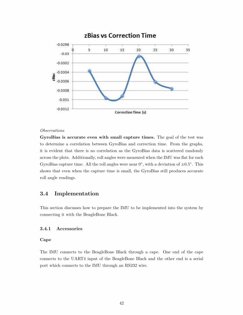
Observations
GyroBias is accurate even with small capture times. The goal of the test was
to determine a correlation between GyroBias and correction time. From the graphs,
it is evident that there is no correlation as the GyroBias data is scattered randomly
across the plots. Additionally, roll angles were measured when the IMU was flat for each
GyroBias capture time. All the roll angles were near 0◦, with a deviation of ±0.5◦. This
shows that even when the capture time is small, the GyroBias still produces accurate
roll angle readings.
3.4 Implementation
This section discusses how to prepare the IMU to be implemented into the system by
connecting it with the BeagleBone Black.
3.4.1 Accessories
Cape
The IMU connects to the BeagleBone Black through a cape. One end of the cape
connects to the UART4 input of the BeagleBone Black and the other end is a serial
port which connects to the IMU through an RS232 wire.
42

RS232
For the IMU to connect to the cape, a serial connection is required as the BeagleBone
Black uses serial communication. An RS232 cable has a serial port on one end which
connects to the BeagleBone Black cape and a Micro-D9 port on the other end which
connects to the IMU. The RS232 cable also provides 5V of power to the IMU through
a transformer. To connect the IMU to a computer using a USB connection, the serial
connection side of the RS232 cable can be interchanged with a USB cable.
3.4.2 BeagleBone Black Setup
The IMU provides information to the bike through the BeagleBone Black. It is neces-
sary to prepare the BeagleBone Black properly before communication with the IMU is
established. Detailed instructions using Unix commands are located in section "Unix
Commands".
Boot File
The IMU is connected to the BeagleBone Black through the UART4 input on the Bea-
gleBone Black. When the BeagleBone Black starts up, the UART4 input is initially
off and must be enabled to turn on automatically. To do so, the uEnv.txt boot file on
the BeagleBone Black must be configured to enable the UART4 input when the Bea-
gleBone Black is powered on. The following command must be added to the uEnv.txt
file located in /boot.
’optargs=quiet drm.debug=7 capemgr.enable_partno=BB-UART4’
Python Libraries
Since the IMU communicates with the BeagleBone Black using serial commands, the
Python serial library must first be installed on the BeagleBone Black. The library is
called ’pyserial’ and can be downloaded from
https://pypi.python.org/pypi/pyserial
Unix Commands
The following Unix commands are used to connect and navigate around the BeagleBone
Black when connected to a Mac or any computer that uses Unix.
43

IP Address of BBB: 192.168.7.2
Copy files/folders from Mac to BBB:
’scp -r pyserial-2.7 [email protected]:’
*adding -r allows to copy folders
ssh to BBB:
sudo ssh [email protected]
Adding RSA keys (middle man attack alert):
ssh to BBB
’ssh-keyscan -t rsa server_ip’
copy starting from “server_ip ssh-rsa. . . ”
‘exit’
navigate to /.ssh on Mac
‘nano known_hosts’
paste rsa key under original key
Editing files in terminal:
‘nano file_name’
Running python program in terminal:
‘python file_name’
Installing pyserial-2.7 on BBB:
downloaded and extracted pyserial-2.7.tar.gz file
navigate to Desktop on Mac
‘scp -r pyserial-2.7 [email protected]:’
ssh to BBB
‘cd pyserial-2.7’
‘sudo python setup.py install’
Removing directories on BBB:
‘rm -r pyserial-2.7’
Check enabled Serial Ports for BBB:
’ls -l /dev/ttyO*’
44

Enable Serial Ports on BBB:
Manually:
’echo BB-UART4 > /sys/devices/bone_capemgr.*/slots’
Automatically On Startup:
Add command to end of uEnv.txt file in /boot
’optargs=quiet drm.debug=7 capemgr.enable_partno=BB-UART4’
3.4.3 Pre-run Procedures
Before each test run, the best procedure would be to run ’Capture GyroBias’ for 10
seconds and have the bike lay still. It was concluded that running ’Capture Gyro-
Bias’ each time would be preferred over manually inputting GyroBias values. Running
GyroBias at the beginning of each run provides the most up to date GyroBias values
since the values are adjusted to the temperature of the sensors. An issue arising with
manual GyroBias was that although the bias was applied instantly and roll angles were
reported immediately, the roll angles took 30 seconds to decrease from 14◦ to the ideal
0◦ when the IMU was placed on a flat surface. Using ’Capture GyroBias’ only requires
10 seconds and provided accurate roll angles and roll rates immediately after ’Capture
GyroBias’ was performed.
45

Chapter 4
Rotary Encoder
Contributors: Eric Huang, Xiangyun (Joyce) Xu, & Rhett Wampler
4.1 Overview
Control of the autonomous bike requires monitoring of the front wheel’s angular motion
and position. The tool chosen for this task is the rotary encoder. A rotary encoder is
an electro-mechanical device which measures the angular motion or position of an axle
and outputs signals (more explained in section 4.2). Once these signals are received, the
front wheel’s position and motion speed can be calculated (more explained in section
4.6).
There are two types of encoders: absolute and incremental. Absolute encoders maintain
the exact position data of what it’s measuring even after powered off, and incremental
encoders express changes in position by tracking movement from an initial starting
point. Both types of encoders can be used with our front wheel motor, but the incre-
mental encoder is a more practical choice since it is easier to measure velocity due to
its nature of measuring changes in movement to determine position. Not only that, but
there is code online that works with incremental encoders, making a baseline design of
the bike more viable with incremental encoders.
In this section, we will review our encoders, the rationale behind our choices in en-
coder, some general useful information about encoders and how they work, how we
used encoders to calculate the position and velocity of the wheel, how to use our hard-
ware, and how to interface with the BeagleBone Black, our microcontrollers.
46

4.2 Basics
As mentioned in the overview section, we decided to use incremental encoders for track-
ing the front wheel due to its inherent property of keeping track of change in movement,
useful for both velocity and position calculations. We use two incremental encoders for
the autonomous bicycle. The first encoder is the HEDR-55L2-BY09 incremental opti-
cal encoder, which is attached to the axle of the front steering motor, and the other
encoder is the Encoder Products Company Model 260 encoder that will be attached
to the bicycle’s front fork. The selection and specifications of these two encoder are
discussed in section 4.4.
The reason for two encoders is that there will be slight slack between the front motor
and its gearbox, meaning that there will be a need to measure the shaft rotations at
the motor and at the gearbox since the gearbox’s rotation might be slightly behind the
motor’s rotation.
Figure 4.1 shows a common form of an encoder and encoder disk. The shaft of a
motor can fit through the hole in the middle, and the silver disc will spin with the
encoder. That disc is the most important part of that typical style of encoder. That
disc has small slits spread evenly throughout, giving us the distance between each slit
(e.g., 4096 slits spread throughout means that each slit is 0.087 degrees apart) . When
the disk spins, the encoder counts the notches as they come by, thus allowing us to
know our position and even velocity (as explained later in section 4.6).
Figure 4.1: Common form of an encoder (left) and an encoder disk (right)1
We chose to use incremental encoders because the BeagleBone Black (BBB) features in-
1Image obtained from http://www.directindustry.com/prod/honest-sensor/product-125247-1568418.html
47

tegrated eQEP module. eQEP, which stands for Enhanced Quadrature Encoder Pulse,
is a translation scheme which allows the BeagleBone Black to interpret the encoder’s
output signals as a change in the encoder’s angle. High quality incremental encoders
(that is, reliable, and providing enough resolution) can be acquired cheaply, so it made
economic sense to utilize the BBB’s eQEP feature.
Both encoders measure the front wheel in order to maximize the accuracy of angu-
lar measurements. Since the bike is balanced entirely by steering action, the increase in
accuracy is worth the additional cost. The encoders have been placed on the steering
motor axle and the front fork because the site of greatest possible error is the interface
between the axle and the fork.
Another way of thinking about this is as follows: the encoder attached to the mo-
tor is for controlling the bike, whereas the one attached directly to the bicycle fork is
for measurement of the bicycle’s state.
4.3 Working Mechanism
Our encoders are incremental rotary encoders that all use the notched discs to count
changes in position, but there are different types of encoders that use a variety of
methods to count these notches in the disc as it rotates. The two kinds of incremental
rotary encoders that use different mechanisms to count the slits in the disc are optical
and magnetic.
4.3.1 Opti-laser based Incremental Encoders
Optical incremental encoders are the most widely used type of rotary encoder. An
optical encoder consists of an LED light source, a light detector, the disk and a signal
processor. As the disk spins, the light shines through the slits on the disk, allowing the
detector to count how many of those slits have passed by (the term used for amount
of slits that passed by is called counts). The encoder’s circuitry then translates the
pattern of light into signals that can be accessed via the Beaglebone Black to obtain
the position information.
4.3.2 Magnetic based Incremental Encoders
Magnetic based incremental encoders are similar to optical incremental encoders, but
the difference is that instead of a light source and a light detector to count the disc
rotating, its disc is magnetized over magneto-resistive sensors that detects the magnetic
48

fields that the spinning disc will generate. When the disc spins, the notches will have
no magnetic fields, so when the notches spin over the magneto-resistive sensors, the
sensors will sense the drop in magnetic field.
Both of the encoders also have an additional output named Index, or "I" channel.
This channel emits a pulse only when a particular point on the disc, called the index
position, passes the detector.
4.4 Encoder Properties
For our purposes, we are concerned with a few properties of the incremental encoders
we are using. They include:
• Resolution, measured in Counts Per Revolution (CPR), which represents how
many transparent slits are on the code disc. A higher CPR corresponds to
greater measurement accuracy because as discussed before, having more slits
spread throughout gives a smaller angle in between each slit, giving us more
accuracy in our positioning since we can detect smaller changes in angle.
• Supply Voltage, which determines both the power source required for the encoder,
as well as the voltage of the output signals. However, encoders available for the
public are usually offered at the 5 volts level.
• Shaft Diameter, which should match or be greater than the diameter of the axle
whose rotation is being measured.
• Differential Outputs allows filtering for noises. Let’s say an encoder has one
output. With differential outputs, it will be the primary output and a complement
output. These two outputs will be subtracted from each other to filter out the
noise that the primary output may be picking up.
For our chosen encoders, these properties are as follows:
HEDR-55L2-BY09 on motor
3600 CPR
5V Supply
8mm Shaft Diameter
optional non-differential or differential output
49

Figure 4.2: Image and of the HEDR encoder with dimensions2
E.P.C. Model 260 on fork
4096 CPR
5V Supply
15mm Shaft Diameter
differential output
Figure 4.3: Image of the Model 260 encoder3
Our team for the Fall 2015 semester chose the second encoder for the fork (the first
encoder was already purchased by previous teams). We chose the 15mm shaft diameter
because the gearbox’s shaft at the fork was that size. We also chose differential output
to filter out noise and make calculations easier later on. We chose 4096 CPR because
it’s enough cycles to give us one hundredth of a degree measurement (more on that
later) and it is also a power of 2 number that is within a reasonable price range. We
chose the model 260 because the company offered a 50 % discount while offering the
above options.
2Image obtained from http://www.avagotech.com/docs/AV02-3823EN3Image obtained from http://encoder.com/products/incremental-thru-bore-motor-mount-
encoders/model-260/
50

4.5 Encoder Outputs
The two optical encoders used in this project have three output channels. They are
the index (Z), channel A (A), and channel B (B). Index is a certain notch on the disc
that defines the 0 ◦ of the encoder, which sends out one signal per revolution. When
encoders have an index, you have to turn the encoder all the way to or past the index in
order to get the encoder to start counting the notches from its relative position.
4.5.1 Quadrature Output
The most common type of incremental encoders use two channels to sense position.
Channel A and channel B are outputs that counts the transparent slits that rotate
by. The reason for for two channels is to determine what direction that the encoder is
rotating in. As seen in figure 4.4, channel A and channel B are 90 ◦ out of phase in the
output of their signals. If A leads B, for instance, the encoder rotates in a clockwise
direction. On the contrary, if B leads A, the encoder rotates in a counter-clockwise
direction.
Figure 4.4: Sample output waveform of channel A an channel B 4
However, having two channels is also beneficial for measurement accuracy. In our Model
260 encoder, we can get 4096 counters per revolution. That’s for one channel, so we
can actually get 8192 counts per revolution.
4.5.2 Counting on the edges
The encoder will send its signals when the Beaglebone polls the encoder for the data.
The Beaglebone will poll the encoder periodically (set by the control code) on its in-
ternal clock. On every clock pulse, the encoder will send the data. One thing to note is
that there is the initial session of the Beaglebone polling the encoder, and there is also
4Image obtained from http://www.ni.com/white-paper/4763/en/
51

the ending session when the Beaglebone is finishing its pulse. These are called rising
edge and falling edge respectively. Encoders can send their data on both edges, thus
doubling the amount of counts it can measure.
That means in our Model 260 encoder example, we found that it can get 8192 counts
per revolution. With the inclusion of both rising edge and falling edge, it can now
count up to 8192 · 2 counts per revolution, or 16384 counts per revolution.
4.6 Angular Speed Calculation
The resolution of encoder heavily influences the accuracy of the speed measurements.
As discussed in the previous sections, having more counts per revolution allows us to
measure smaller degrees per counts, thus giving us a higher accuracy on position mea-
surement and even velocity measurement (discussed soon).
Applying the calculations in the Encoder Outputs section, the HEDR-55L2-BY09 en-
coder used in this project has a resolution of 3,600 CPR. With a four-fold increase in
the resolution provided by the quadrature output, we get 14,400 counts per revolution.
Applying the same method to the Model 260 encoder gives us 16,384 counts per revo-
lution. Therefore, the minimum angle of rotation that can be detected by the HEDR
encoder is 360 ◦ divided by 14,400 counts or 0.025 ◦ per count. For the Model 260
encoder, it’s 0.0219 ◦ per count.
Measuring the velocity and position via the encoder is straightforward after getting
the counts. Using the Model 260 encoder as an example, we know that it’s 0.219 ◦ per
count. If we poll the encoder and find that in the last 0.5 s since we last polled, we
went from + 4100 counts to + 4110 counts (relative to index), then we know that we
went from 4100 · 0.0219 ◦ (89.79 ◦) to 4110 · 0.0219 ◦ (90.009 ◦). We can also determine
velocity by taking the difference (90.009 ◦ - 89.79 ◦ = 0.0219 ◦) in half a second. That
means the angular velocity was 0.0219 ◦
0.5s= 0.438 ◦/s.
The classical and probably the simplest method to approximate the angular speed
of the encoder is to directly measure the frequency of the encoder pulses by counting
the number of pulses in a constant period of time, which will output a discrete mean
angular speed in each polling period. The mathematical representation of this method
is shown below:
ω =dθ
dt≈
∆θ
∆t=
60 · 2π · ∆N
Tpolling ·Np
[rpm]
52

where Tpolling is the polling period of the Beaglebone black set by the code, ∆N is the
number of pulses detected in one polling period and Np is the number of pulses per
revolution (four-fold increase in resolution after quadrature decoding).Therefore, if the
polling period is set to 0.01 s, the minimum motor speed that can be detected by the
HEDR encoder using this method is 2.62 rpm, and the Model 260 encoder can detect
a minimum angular speed of 2.30 rpm. While the theoretically detectable minimum
angle of rotation is 1
Np
, the detection of only 1 pulse ,which approaches the limit of the
capability of the encoder, is usually inaccurate. Usually, measurements larger than 10
pulses in one polling period can be considered accurate. Therefore, the actual reliable
minimum speed that can be detected using this method (with a 0.01 s polling period)
is 26.2 rpm by the HEDR encoder, and 23 rpm by the Model 260 encoder. When
dealing with low-speed rotation, a commonly adopted way to improve the accuracy
is to increase the polling period, for example, to 0.1 s, but this method reduces the
bandwidth of the Beaglebone black.
An alternative method to reduce the measurement errors at a certain level of of low
speed is to measure the time elapsed between successive encoder pulse count. The
speed calculation is shown below:
ω =dθ
dt≈
∆θ
∆t=
2π · 60
Np · ·∆t[rpm]
The accuracy of this method suffers from the opposite limitation, as does the first
method. A combination of a possibly high motor speed and high resolutions of the
two sensors used in this project, the time elapsed between two successive encoder pulse
counts, ∆T , is expected to be very small, which greatly relies on the resolution of
the internal timer in the Beaglebone black.For example, if both encoders used in this
project rotate at 5 rpm, the time elapsed between two pulses is about 0.5 ms. For
accuracy time measurements, the resolution of the internal timer must be higher than
0.05 ms.
4.7 Encoder Functionality Test
The functionality of an encoder can be tested with an adjustable voltage supply and
an oscilloscope. The fowling method is the simplest to determine if the hardware of the
encoder work correctly. Both encoders used in this project require a 5 V voltage supply.
Therefore the +5 V and GND connection points of the encoder should be connected to
the voltage supply. Then channel A and channel B of the encoder should be connected
to channel 1 and channel 2 of the oscilloscope. Once the encoder is powered on and
53

rotating, the two channels of the oscilloscope will displace two square waveforms 90 ◦
out of phase. The output frequency will also be displayed on the oscilloscope.
4.8 Encoder Circuit
Wiring the encoder to the Beaglebone will require some additional hardware. One of
the main reasons is that the encoder runs at the industry standard’s 5 volts while the
Beaglebone’s ports for the encoder run at 3.3 volts. Not only that, but since one of
our encoders come with differential lines (output line and its complement), we will also
need some hardware that will subtract the two to filter the noise out for us. The two
hardware we will need will be the differential line receiver model ST26c32AB and the
optoisolator 5V to 3.3V IL711, both found on digikey.
4.8.1 Differential Line Receiver
A differential line receiver takes in two signal lines and subtract the two to filter out
noise. This is beneficial for the primary line when it’s getting background noise. It will
get a huge spike to represent that it picked up when its designed function happened
(push of a button, etc.). The secondary line is designed to simply get the background
noise of the primary line too. By subtracting the two, the output data should ideally be
all zeroes and then that value when the spike occurs. As seen in figure 4.5, we use the
differential line receiver (the ST26c32AB). It has ports for 4 sets of lines, and because
only our fork encoder has the differential line option, we only use up 3 sets of them
(channel A, channel B, and index).
4.8.2 Opto-isolator
In electrical circuits, you cannot mix different voltage items with each other because
they can break (it’s like trying to force a 5 inch object into a 3 inch slot). As mentioned
before, the encoder runs at 5V lines. However, the Beaglebone sensor ports are slated
for 3.3V. In order to solve this issue, we use an opto-isolator which transfers a signal
between elements of the circuit while keeping them electrically isolated from each other.
With this opto-isolator, we can feed in a 5V encoder signal line into, and we can then
get the 3.3V signal line that can then go into the Beaglebone. The opto-isolator chips
we ordered can only take in two lines per chip, so we use three separate chips for both
encoders (each encoder has 3 signal lines each that need to be converted to 3.3V).
The opto-isolators are shown in figure 4.5 when the channel A, channel B, and index
lines from both encoders are fed in, isolated for 3.3V lines, and then connected to the
Beaglebone.
54

Figure 4.5: Wiring schematic for both encoders to Beaglebone using differential linereceiver and optoisolators5
55

4.9 Connection to the Beaglebone Black
Each encoder has five connection points to the BeagleBone Black: 5V and GND, chan-
nels A and B, and channel I. Each of BeagleBone Black’s three eQEP modules, each
of which corresponds to a set of input pins (for channels A, B, and I), while 5V and
GND are general purpose output pins that can be found from the BeagleBone Black’s
general pinout diagram. The three eQEP modules have four available pinouts, which,
in the eQEP driver code, are referred to as eQEP0, eQEP1, and eQEP2 and eQEP2b,
both of which connect to the same eQEP module.
Under our current configuration, the HEDR encoder uses eQEP0, which corresponds to
P9_42 for channel A, P9_27 for channel B, and P9_41 for channel I. The BeagleBone
Black’s UART interface occupies the odd pins between P9_1 and P9_15, and so the
E.P.C. Model 260 will have to be attached using eQEP2 or eQEP2b, which both use
pins on P8. The pins for each particular layout can be found and modified in the eQEP
driver code, which will be explained in the eQEP section under Code.
4.10 Alternatives
It is important to note that there are other methods of measuring the position of the
handlebar, and one of the main alternatives is using a potentiometer.
4.10.1 Potentiometer
The potentiometer is an adjustable resistor that can give us varied voltages. In the
classic equation where Voltage (V) is Current (I) times Resistance (R), or V = I * R,
our bike is set up to provide a constant current thanks to our power supply. With I
constant, that means that our Voltage will be directly proportional to our Resistance.
By adjusting our potentiometer and knowing how much we adjusted it by, we can see
how much the voltage has changed by too. The contra-positive also works too; if we
know how much the voltage has changed, then we know how much the potentiometer
has changed.
How Potentiometer Works
The previous team used a potentiometer to measure the position of their encoder. The
potentiometer they used was a turn-based potentiometer where turning the knob on
5Self created image5https://en.wikipedia.org/wiki/Six_degrees_of_freedom/media/File:6DOF_en.jpg
56
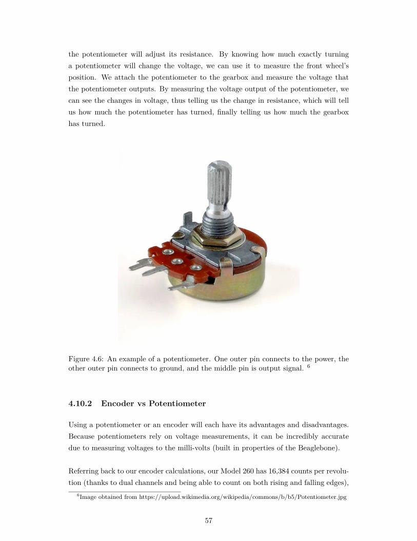
the potentiometer will adjust its resistance. By knowing how much exactly turning
a potentiometer will change the voltage, we can use it to measure the front wheel’s
position. We attach the potentiometer to the gearbox and measure the voltage that
the potentiometer outputs. By measuring the voltage output of the potentiometer, we
can see the changes in voltage, thus telling us the change in resistance, which will tell
us how much the potentiometer has turned, finally telling us how much the gearbox
has turned.
Figure 4.6: An example of a potentiometer. One outer pin connects to the power, theother outer pin connects to ground, and the middle pin is output signal. 6
4.10.2 Encoder vs Potentiometer
Using a potentiometer or an encoder will each have its advantages and disadvantages.
Because potentiometers rely on voltage measurements, it can be incredibly accurate
due to measuring voltages to the milli-volts (built in properties of the Beaglebone).
Referring back to our encoder calculations, our Model 260 has 16,384 counts per revolu-
tion (thanks to dual channels and being able to count on both rising and falling edges),
6Image obtained from https://upload.wikimedia.org/wikipedia/commons/b/b5/Potentiometer.jpg
57

making each count cover 0.0219 degrees per count. The accuracy of the encoder is a
magnitude of ten worse than the potentiometer. However, the encoder is easier to work
with.
As described earlier, there are already coding libraries online that allow us to work
with the encoder easily. We simply have to get the counts from the encoder and plug it
into our equation to get the position. Not only that, but the encoder is already being
used by the previous team for the motor. Attaching an encoder to the fork would be
more convenient than using a potentiometer because we could use the same circuit as
the motor’s encoder and also use the same code to read off of the new encoder.
58

Chapter 5
Code
Contributors: Eric Huang & Rhett Wampler
5.1 Overview
Our BeagleBone Black runs on a version of the Debian OS that has been adapted for
multiple BeagleBone products. The default BeagleBone Black OS is the Angstrom
package, but it was replaced during the effort to fix an issue with the eQEP encoder
driver. The code for our project is fairly high-level, so both operating systems should
serve equally well. However, we currently have chosen to run on Debian, since Debian
possesses a greater amount of online literature.
When logging into the BeagleBone Black, the Autonomous Bike Team uses the "root"
username. Thus far, programming has occurred in two distinct areas: control code
and system code. Control code, as the name implies, refers to those programs, written
entirely by the team, that carry out control functions for the bike; in short, receiving
and interpreting sensor data, decision-making, and outputting signals to the motors.
System code represents modifications made to the vanilla Debian system in order to
meet the needs of our control code. All control code is written in Python and can
be found in the "/ABT/" directory under the "root" user’s home directory. System
code has been implemented for three areas so far: the eQEP driver, the UART-to-IMU
connection, and a set of programs called ADAfruit_BBIO, all of which will be further
explained in the "System Code" section.
59

5.2 Control Code
The main control file for the BeagleBone Black is the "sensor monitor.py" file. It de-
pends upon the files "pid.py", "eqep.py", "imu.py", and "openLoop.py", and also upon
the Adafruit_BBIO libraries. The other files are throwaway test files written to de-
velop and troubleshoot individual sections of the bicycle’s circuitry. The main control
program works in a loop: first it pulls information from the encoders and the IMU,
then it uses a linear equation to calculate in which direction and how fast the front
steering motor should turn in order to keep the bike stable.
There is also a separate part of the control program which monitors the sensors and
kills power to the bike if any of the sensors go haywire. When ensuring that the en-
coders are working properly, the monitor looks at both encoders at once. It checks the
differences in the output between the two encoders, and if the difference is greater than
the threshold set by the user, then it kills the bike. The second part of the monitor is
ensuring the IMU is working properly. The monitor will kill the bike if the bike’s lean
angle is ever past the threshold because at that point, it’s almost impossible for the
bike to recover. In our case, we set the lean angle max to 45 degrees (as suggested by
Professor Ruina).
The following flowchart shows the full structure of "sensor monitor.py", which is the
most recent version of the control code.
60

The "imu.py" program translates raw data coming from the IMU into recognizable
values, such as roll angle and rate, which "sensor monitor.py" can then use in its cal-
culations.
61

The "openLoop.py" program initializes and maintains power to the front steering motor.
It contains code which converts the target angular velocity of the steering motor, which
is periodically calculated by the main body of the control code, into a duty cycle output.
The "eqep.py" program streamlines the interface with the eQEP drivers, and allows
the control code to treat each instance of eQEP as an object containing encoder values
and operating modes that can be both viewed and modified.
The function "calculate()" is defined in the main body of the control code. "calcu-
late()" takes in the bike’s lean angle, lean velocity, and current steering angle, and uses
a linear equation to output the velocity at which the steering motor should turn in order
to stabilize the bicycle. The linear equation uses three coefficients, labeled k1, k2, and
k3, which are the result of testing and modeling by the previous semester’s team. Note
that the coefficients were specifically developed for bike stabilization, rather than nav-
igation. In the future, when the control code begins to include navigation (purposeful
changes in direction) as well as stabilization, new coefficients will have to be developed
in order to stabilize cases such as a deliberate right or left turn.
The "pid.py" program represents the original control framework, the functions of which
have since been divided up between the other control programs. Currently, no part of
"pid.py" is used by the control code, although parts of it could be helpful for future
development.
The Adafruit_BBIO libraries will be explained in the next section on System Code.
5.3 System Code
Thus far, system coding has taken place for the eQEP driver, the UART/IMU connec-
tion, and for a set of programs called the ADAfruit_BBIO libraries.
5.3.1 eQEP driver
The eQEP module is the decoding unit to get position and direction information from
the incremental encoders. The built-in eQEP Linux kernel in the Beaglebone Black
is from Texas Instruments (TI). The eQEP driver used on our BeagleBone Black was
developed primarily by Nathaniel R. Lewis, whose Github username is Teknoman117.
Specific instructions for acquiring the driver can be found in the "Code" folder of the
Autonomous Bike Team’s Google Drive, but we will note here that the BeagleBone
Black, having loaded a driver during one active session, will not necessarily remember
62

to keep the driver active from that point onward. In order to have a driver become
active whenever the BeagleBone Black is turned on, a startup script must be added
to the "/boot/uEnv.txt" file. Again, specific instructions can be found in the Google
Drive’s "Code" folder.
The eQEP driver assigns a set of pins to one of the BeagleBone Black’s eQEP mod-
ules. When channels A, B, and I of an encoder are connected to the corresponding
BeagleBone Black pins, the eQEP module and driver translate the incoming signals
into an increase or decrease of a variable that represents the angular position of the
encoder. For example, depending on the configuration of channels A and B, an in-
crease in the variable could represent counterclockwise motion, while a decrease in the
variable represents clockwise motion. Since there are two encoders, whichever direction-
to-variable-change relationship is chosen should be kept consistent in order to simplify
future coding.
Channel I, by default, resets the variable to zero whenever the encoder’s index po-
sition is passed. Ideally, the encoder would be placed such that the index position
corresponds to the front wheel being perfectly in line with the bike. In reality, while we
can place the encoder into position as carefully as possible, there will always be a small
offset between the encoder’s index position and the front wheel’s zero position. The
way to remedy this is to measure the offset manually, then modify the eQEP driver
so that the channel I input sets the front wheel’s position variable to the offset angle
rather than zero.
It is important to note that since both encoders are incremental, the position vari-
ables will automatically regard as zero the position the encoders were in when the
BeagleBone Black is turned on. Therefore, each time the autonomous bike is turned
on, the front wheel must pass the index position of the encoders before the position
variables will reflect the actual position of the front wheel.
The eQEP driver has a list of commands that make it easy to use the encoder to
control the motors. In the control code, after creating a certain eQEP encoder, you get
access to the encoder’s properties such as its period and position. Simply calling on
functions such as get_period() or get_position() will get the values from the encoder.
The entire function list can be found on Teknoman117’s github account in his encoder
API folder.
63

5.3.2 UART Interface
The Inertial Measurement Unit connects to the BeagleBone Black via a UART inter-
face. The BeagleBone Black does not have a specific UART port, but it does have
a ready-made driver which assumes control of the odd-numbered pins between P9_1
and P9_15. The process to activate this connection whenever the BeagleBone Black is
turned on is similar to the process for activating eQEP. In the "/boot/uEnv.txt" file,
there are many commented lines of code which, when un-commented, activate major
functions of the BeagleBone Black’s "capes", which is another name for pin configura-
tions designed to handle certain interface types. One such line of code activates the
UART cape; simply un-comment the line in order to activate UART (however, make
sure to un-comment the line that pertains only to UART, as activating other capes can
cause pin allocation issues with the eQEP drivers.
After the pins have been allocated, an Adafruit_BBIO function (described in the
next section) for UART simplifies integration of the UART connection into our control
code.
5.3.3 ADAfruit BBIO
The ADAfruit_BBIO libraries, also referred to as the IO Python Libraries, are code
designed to simplify usage of the BeagleBone Black’s IO pins (as the name "BBIO" im-
plies). The libraries are broad, and feature many useful expansions of the BeagleBone
Black’s capabilities. A full listing of the ADAfruit_BBIO library can be found online,
as well as thorough installation instructions.
We utilize the ADAfruit_BBIO PWM program in our control code in order to output
variable duty cycle square pulses to the bicycle’s motors. The square wave signals,
emitted at high frequency, allow the BeagleBone Black to simulate an analog, variable
voltage output, which the motors use to control power.
Adafruit_BBIO ADC allows the BeagleBone Black to read the DC voltage of a speci-
fied pin. This function helps to interpret the input from analog voltage output sensors.
Since the potentiometer has been phased out of the autonomous bicycle’s design, ADC
does not currently play a role in bicycle control. Nonetheless, it is a helpful feature.
The Adafruit_BBIO UART package allows information from the BeagleBone Black’s
UART cape to be easily usable in a Java environment. The program is used by the
control code to quickly pull information from the Inertial Measurement Unit.
64

The setup is very simple; once the ADAfruit_BBIO libraries have been installed on
top of the BeagleBone Black’s vanilla Debian OS, control programs can be written with
headers that load up whichever ADAfruit_BBIO utilities are required. Then, the con-
trol program can call new programs and functions, such as PWM() or ADC, which can
simplify any program that uses pins (which is most of them). Other ADAfruit_BBIO
utilities could prove useful in the future, but for now we use a very limited number.
Any use of the libraries is signaled at the head of a control code, by the line:
"import Adafruit_BBIO.name as name"
65
Chapter 6
Front steering and MechanicalDesign
Contributors: Olav Imsdahl & Rannie Dong
6.1 Overview
The front steering needs to be sturdy and reliable in both the mechanical and sensor
aspects. We want the sensors to accurately read the steering angle and also the motor to
turn the wheel without much error. There were many problems that the front steering
mechanism had that had to be fixed. The fork insert was not fitted tightly so it wiggled
a little bit. The steel plate that is connected to the bike is not welded orthogonal to
the steering axis making the rods that hold the motor and encoders not sit perfectly
aligned with the steering axis. In addition, the distance between the rod holes on the
steel plate and the holes on the circular discs that slide onto the rods have different
distances. We also ordered a new encoder which should sit below the coupling around
the shaft leading from the fork.
Other than the problems with the front steering, we had to move the IMU sensor from
inside the ammo can at the back to a sturdier position on the bike frame. It was also
recommended to design and attach a start-and landing-gear to the bike so that it can
start and stop without crashing. These fold-able wheels should keep the bike upright
when it is not moving and fold up when we are testing the bike. There is also the
option of making the bike not fall over when it is brought to a controlled stop.
66

6.2 Front Steering
Figure 6.1: front steering overview
One of the most important parts of the bike is the front steering in that it is vital to
keeping the bike upright. It is important to know the accurate position of the front
wheel and to be able to control it well. The front wheel is controlled by a motor which
is in line with the steering axis. It is connected by a coupling and has two encoders
measuring the angle of the wheel. There is one below the coupling which should not
have much of an error as it is directly connected to the wheel. The other encoder on
67

the back of the motor is connected through gears and the coupling to the wheel which
could account for some error.
6.2.1 Fork Insert
Figure 6.2: front wheel with fork insert and coupling
The bottom most part connects the fork to the encoder and fits into the bottom half
of the coupling. It sits tightly inside the fork tube and is kept from rotating by a bolt
68

that passes through at the bottom near the top of the wheel. The top end of the insert
is 15mm in diameter and fits through the encoder into coupling.
6.2.2 Orthogonal plate
Figure 6.3: plate connected to steel on the bottom and holding the 4 long rods
The plate above the steel ring (which is brazed to the bike) accounts for the offset of
the steel part. it can be levelled by changing the lengths of the 4 bolts. This ring is the
base of the whole steering mount and should align all of the long 1/4-20 rods. The 4
69

bolts holding the ring have a distance of 2.5in and the distance between the long rods
is 2.25in.
6.2.3 Coupling
Figure 6.4: the coupling between the motor (top) and the encoder (bottom)
The coupling connects the wheel and encoder part with the top half which includes the
motor and the back-encoder. The Nylon piece between both coupling parts can account
for an off-set between the bottom and top half in the horizontal direction. It doesn’t
70

account for any off-set angle between the wheel axis and the motor axis. That’s why
it is important that the individual plates along the 4 rods are parallel to the bottom
plate.
6.2.4 Encoder on the back
Figure 6.5: the encoder (black box) sits on the end of the motor
The back encoder was difficult to mount and adjust because the screws connecting the
plate to the back of the motor were in the way of the encoder to sit on the rear pin
71

correctly. It is important to have plate on the back centered with the motor to keep
the sensor from rubbing. To solve this problem I had to counter-sink the screws to be
able to attach the encoder.
6.3 Inertial Measurement Unit mount
Figure 6.6: the IMU mount is clamped to the bike frame (blue)
Originally the IMU sensor was placed inside the ammo can at the back of the bike, which
introduced many possible factors for inaccurate readings. Not only would it have to
be mounted securely inside the can, but the can itself would have to be constrained
to minimal movement with respect to the bike frame. Another complication was that
any dynamical modeling would have to consider that the angle and angular rate data
created during tests of the bike were taken from said unknown and unstable point at
the back of the bike. For these reasons, the sensor had to be connected to the bike
frame itself to let us measure the angle and rotation of the bike. It had to be placed
in a spot where it would most accurately measure the changes in angle and angular
rate and still be protected during a crash. Also necessary was a horizontal position for
measurements that correspond to what the IMU code expects, so that we ensure the
correct angles are taken in by the controller code. A suitable place was found right in
front of the bike seat on the top tube, where the tube splits into a fork. This allowed
for attaching a plate horizontally to the ground as well as preventing movement in the
lean and yaw angles. Most satisfactorily, the positioning is now closer to the center of
the bike and centered along the bike’s lengthwise axis.
The design for the mount consists of two machined plates that clamp onto the bike (by
72

way of long screws) and sandwich the fork of the top tube between them. Threaded
holes in the top plate allow us to screw the sensor into place. The IMU is easily
removable by removing the screws and the port for the connector cable is accessible
on the back facing side. A notable feature of the mount are the grooves running front
to back which are concentric with the tubes. They ensure that the plates do not slide
with respect to the tubes given that the screws are tightened properly.
6.4 Foldable starting and landing gear
Figure 6.7: wheels, gear and motor connected to bike
73

Figure 6.8: reverse side with end-stops
This feature is not critical to the success of the bike but is an added feature that will
help facilitate testing. Wheels on the side of the bike help to keep the bike steady at
the beginning of testing. However we don’t want them keeping the bike upright during
testing so they must be folded upwards during this time. It would also be useful if
they can be folded down again so the bike can be brought to a stop without having to
crash-land or be caught every time. One important feature is that there is no sensor
to give feedback when the wheels are fully folded up. Instead there are end-stops that
turn off the power supply when it has reached it’s ends. By connecting diodes to the
74

end-stops the current will only flow through one of the end-stops which is then turned
off once the motor reaches the end.
Figure 6.9: circuit with end-stops
Once one of the end-stops is triggered the current can only flow through the other one
to turn it in the other way.
75

Chapter 7
Printed Circuit Board Design
Contributor: Weier Mi Editor: Eric Huang
7.1 Overview
7.1.1 Printed Circuit Board
The printed circuit board (PCB) is a customizable circuit board that allows us to
organize and manage many of the electronic components on the autonomous bike. It
gives us the capability to dictate how to bunch components together for easier and
cleaner wire management, power distribution, and signal management. We could treat
a PCB as a blackbox; we don’t have to know anything about what is happening within
the PCB when it is working, as we don’t know about what’s going on within the
Beaglebone Black (BBB) when it is running our program. We only need to plug wires
from various components, such as encoders and the BBB, to the PCB.
Although the PCB seems to be a good approach for our circuit board, you might
ask: why not use a introductory breadboard with lots of holes for easier removal and
additions of electronic components? What is the point of the extra work on designing
a more integrated circuit board? There are a few reasons. Firstly, the connections on
the breadboard are not as secure as those on a PCB. Wires and pins of components
on the breadboard are exposed to the outside, making them vulnerable to external
forces, such as vibrations from the bike shaking them loose. Also, the wires could age
and crack, even pop out of sockets, causing the circuit board to malfunction and fry
components. Moreover, the breadboard could take up more space than a PCB does due
to the exposed wires and the breadboard being physically larger. Another disadvantage
of the breadboard is that it is more difficult to distinguish between wire connections.
If multiple wires pop out at the same time, we might spend a lot of time on finding the
76

Figure 7.1: Printed Circuit Board.1 Figure 7.2: Breadboard.2
origins and destinations of the wires.
A PCB solves all these problems with its soldered connections to prevent any exposed or
loose wires. By using solder to fuse wires onto our PCB (hence soldering), our wires will
not be prone to shaking loose or folding and breaking. The relatively small size of the
PCB is also an advantage, since the space available on the bike is limited. Additionally,
PCB is fully customazible in area, dimensions, etc. meaning that we will not have to
worry about mistaking wires and ports due to poor organization. Because PCBs are
customizable, we can label the names of ports and components on the top surface of the
PCB, preventing any mistakes when connecting wires to their proper places. Naturally,
the PCB becomes the best solution to this project’s circuit section.
7.1.2 Through-hole versus Surface-mounting
On the PCB, we are using two technologies that components are built with: the
through-hole technology and the surface-mount technology (SMT). These technolo-
gies define how components are built and how they are supposed to be installed on the
circuit board. Components built with the through-hole technology are very common
because it’s a bigger size and is more traditional: all the pads (places to solder the
pins) are meant to be drilled vertically throughout the board. This means that when
connecting through-hole components, we simply fit it all the way through until the
pins clear the hole, and we simply solder those pins onto the board. Not only that, but
through-hole components can simply be attached onto breadboards.
The SMT, however, are not as common as the through-hole because components made
with SMT are so small that they don’t fit on common breadboards. The SMT tech-
nology is a more modern and aggressive approach. It utilizes only less than half the
2"MOS6581 chtaube061229" by Christian Taube - Own work. Licensed under CC BY-SA 2.5 viaCommons - https://commons.wikimedia.org/wiki/File:MOS6581_chtaube061229.jpg#/media/File:MOS6581_chtaube061229.jpg
2"Breadboard" by en:User:LukeSurl - en:Image:Breadboard.JPG. Licensed under CC BY-SA 3.0 viaCommons - https://commons.wikimedia.org/wiki/File:Breadboard.JPG#/media/File:Breadboard.JPG
77

Figure 7.3: Through-hole resistor.3
Figure 7.4: Surface-mount capacitor.4
thickness of the board, and thus allows us to solder components on both sides of the
PCB, although increases the difficulty to solder them. The major advantage of ap-
plying SMT is that devices built with it could be incredibly small, and we could save
a lot more space on the circuit board than if we used through-hole components. For
this project, we will mix up both technologies. We already own most of the parts that
are built with through-hole technology, and we purchased line receivers that are built
with SMT. We believe that by mixing components with components already owned
and purchased ones, we can develop a baseline design to prove that our concept works
before working on improving size and efficiency of the PCB.
7.2 Design Software
7.2.1 Introduction
We decided to use Eagle CAD as the tool to design our printed circuit board. We chose
it because it is very widely used across the world, and we are likely to find libraries that
contain electronic components we want online. If we want to add a certain component
with specific pins and layouts, we would more likely find it in Eagle CAD’s library (due
to its popularity) and simply import and place it in our file. Not only that, but Eagle
CAD is also well-designed and easy for beginners to learn and use. For example, it has
built-in command lines which help us access to the commands we need quickly such as
cloning components. For the board layout design, it also has a tool (Autorouter) that
wires the connections automatically.
Eagle CAD mainly has four interfaces that we used for this project: Project, Schematic,
4"Resistors (1)" by Original uploader was Cyp at en.wikipedia - Trans-ferred from en.wikipedia; transferred to Commons by User:Sfan00_IMG us-ing CommonsHelper.. Licensed under CC BY-SA 3.0 via Commons -https://commons.wikimedia.org/wiki/File:Resistors_(1).jpg#/media/File:Resistors_(1).jpg
4"SMD capacitor" by Alex Khimich - Own work. Licensed under CC BY-SA 3.0 via Commons -https://commons.wikimedia.org/wiki/File:SMD_capacitor.jpg#/media/File:SMD_capacitor.jpg
78
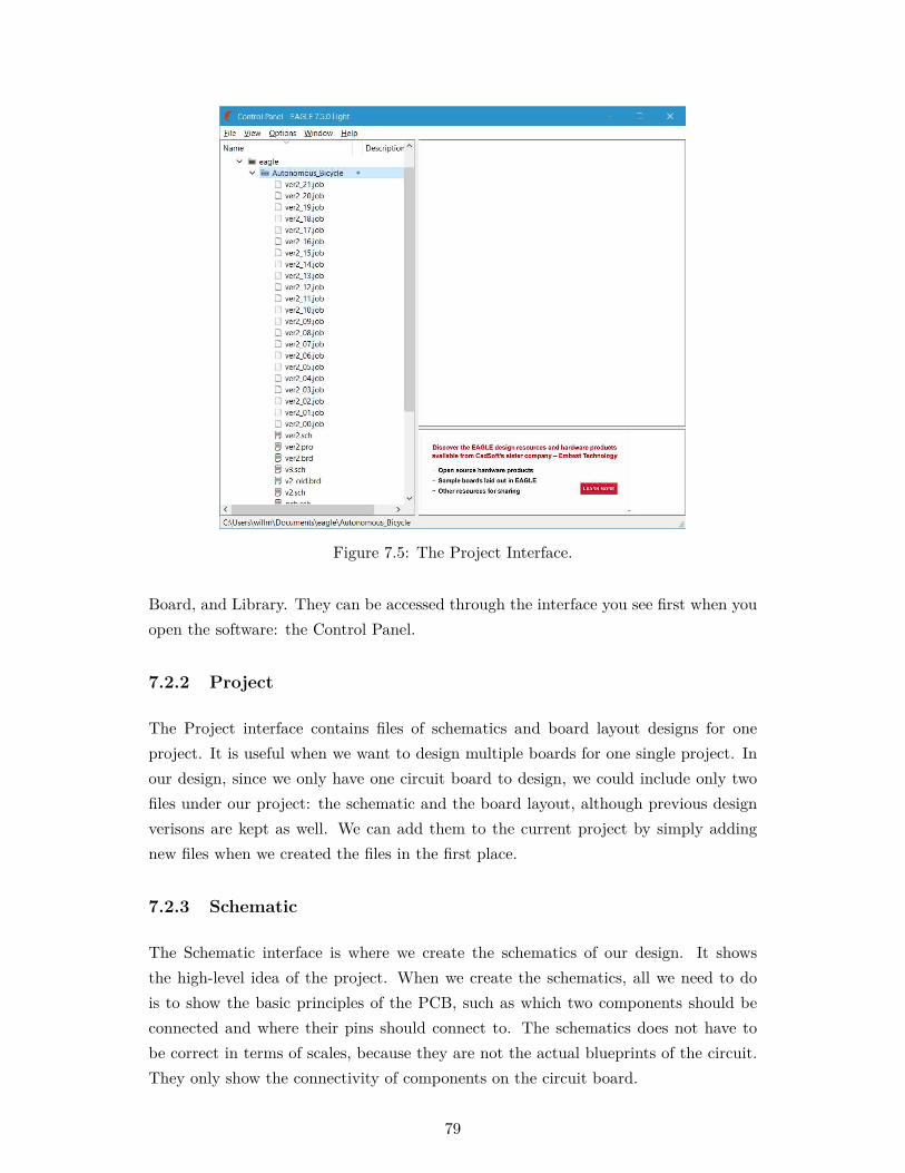
Figure 7.5: The Project Interface.
Board, and Library. They can be accessed through the interface you see first when you
open the software: the Control Panel.
7.2.2 Project
The Project interface contains files of schematics and board layout designs for one
project. It is useful when we want to design multiple boards for one single project. In
our design, since we only have one circuit board to design, we could include only two
files under our project: the schematic and the board layout, although previous design
verisons are kept as well. We can add them to the current project by simply adding
new files when we created the files in the first place.
7.2.3 Schematic
The Schematic interface is where we create the schematics of our design. It shows
the high-level idea of the project. When we create the schematics, all we need to do
is to show the basic principles of the PCB, such as which two components should be
connected and where their pins should connect to. The schematics does not have to
be correct in terms of scales, because they are not the actual blueprints of the circuit.
They only show the connectivity of components on the circuit board.
79

Figure 7.6: The Schematic Interface.
7.2.4 Board
The Board interface is where we deal directly with the board itself. It is completely in
scale, which means the area a component takes on the grid of the board layout is the
same as the area a real component would take on a real PCB, unlike the schematics. In
this interface, we are able to place components anywhere we wish on the board, and we
can connect them by placing wires between designated pins. In the real PCB, the wires
should be internally built. However, there is one thing that we need to keep an eye on:
we should minimize the occurrences of jumper wires; we should try our best to clear
them out. A jumper wire is still a wire that connects two pins, but it is placed outside
the board. It appears when the design fails to arrange a normal internal wire to connect
the pins. Jumpers should be eliminated, because they are exposed to the outside and
they are not as secure as internal wires. It is also feasible for us to eliminate the jumper
wires, because we actually have two layers in the PCB, a top layer and a bottom layer
that enable two wires to cross, but placed in two layers vertically. If we manage the
design carefully enough, there should be a layout solution that does not include any
jumper wire. A built-in tool, named Autorouter, could help us build up a number of
layout solutions while following all the preset design rules, such as not having un-wired
ports or un-determined values for components like capacitors. We could simply pick
one of the solutions, although it could include some jumper wires that are possible
to be fixed manually. In our board layout, we made sure that all jumper wires were
80

Figure 7.7: The Board Interface.
eliminated.
7.2.5 Library
The Library interface enables us to create or edit a library. A library in Eagle CAD
contains one or multiple components, each with different sub-models and technologies,
such as through-hole and surface-mount technology (SMT). Those components have
three sub-interfaces: Package, Symbol, and Device. Package is the part that displays
the actual, in-scale component model. For a component, what we see in Package is the
same as what we deal with in the board layout design. Symbol, on the other hand, is
the part that is not necessarily in-scale, and when we create schematics we place the
Symbols of components. Device is the part that combines Package and Symbol – it
connects pins defined in Package to pins declared in Symbol. We don’t interact with
Device when we create the schematics or board layouts, but we do when we create a
custom component in a library. For some of the components that we are using, such
as the line receiver and the connectors, we can simply utilize existing libraries that are
either built-in in the Eagle CAD or somewhere online. Although Eagle CAD already
comes with hundreds of components, it also happens that the component we want to
use is not included. In that case, we will have to build our own libraries.
To build our own libraries, we could either start with building the Package or the Sym-
81

Figure 7.8: The Library Interface.
bol. Building the Package requires carefully reading the datasheet of the component
that we desire to build, especially the mechanical data that contains information on
the component’s dimensions and pin locations. Since it is exactly in-scale, if we make
a mistake here, the actual component might not fit in the printed board.
We can be a little more casual about building the symbol, because it only displays some
high-level information of the component, which is what pins it has and what compo-
nents these pins are connected to. We can set a random size and random pin locations
of the component, but we should make sure that all pins we could use are included in
the symbol.
After building the Package and Symbol, we combine them in Device by connecting
individual pins defined in the previous two parts, since they are actually independent
to each other. Symbol and Package both point to the same component, so each pin in
the symbol should be directly related to a pin in package. Connecting pins that are
supposed to be the same wraps up this step.
Then, in the Schematic interface, we can access to the component by “using” (it means
importing; in the software click “USE”) and “adding” (click “ADD”) the library and
select the component. We should be able to get the Symbol we just built. After finish-
ing the Schematics we will want to go to Board to start working on the board layout,
and packages of components that we have should appear automatically.
82

Figure 7.9: A built package of Pololu MotorController.
Figure 7.10: A built Symbol of Pololu Mo-tor Controller.
Figure 7.11: A built Device and pin connections of Pololu Motor Controller.
83

7.3 Printed Circuit Board Components
After independent researching, discussing with teammates, studying works from the
previous team, and getting the many valuable suggestions and help from Jason, we
have decided to include the following components in our PCB design:
7.3.1 Delta DC/DC Converter
We are using a battery pack that provides a 24V direct current (DC) power supply to
the entire bike. As a result, we would want to have a voltage converter that transforms
the power output from the battery to a lower voltage since many electronic components,
such as the encoders and many components on the PCB, take a 5 V DC voltage input.
This converter provides a regulated, isolated power supply to the delicate electronic
components that may function wrongly if the input voltage changes dramatically.
We chose this Delta DC/DC Converter (DH06S2405A) because its input voltage is
ranged from 18 to 36 V, with a mean of 24 V, which is the same as our battery’s
output voltage level. Its output voltage level is 5 V, which meets other components’
power supply requirements. Also, it has functions such as short-circuit protection and
overload protection that could make the entire system more secure. Short-circuit pro-
tection would prevent current overflowing and flooding the components while overload
protection would protect too much voltage from accidentally going to the components
and frying them. This converter comes highly recommended by usage of the previous
team and also from one of our mentors, Jason.
The DH06S2405A takes a high voltage input (in our case 24V) and produces a constant
5V voltage output that is isolated from the high voltage. Encoders, the Beaglebone,
and other components that are slated for 5V will use this converter.
7.3.2 Opto-isolator
The Beaglebone pins are 3.3V, but the encoder and other electronical components are
5V. In order to allow the encoder and other components to feed into the Beaglebone
without breaking due to voltage mismatch, we use an opto-isolate circuit. The opto-
isolator circuit works as a physical signal barrier which isolates some components to
others by protecting components from voltage surges. In our bike project, we would
want to use opto-isolators in the middle of transmissions between the Beaglebone Black
(BBB) and sensors or motor controllers. Each of the signals is transferred with a low
voltage level (3.3 V), and the isolator circuits could protect the signal receivers from
voltage surges. But the main function of the opto-isolators is actually transforming
the signals’ voltage level from 5 V to 3.3 V, which matches the requirement of the
84

Figure 7.12: The overall schematic.
85

Figure 7.13: Delta DC/DC Converter in the Schematics.
BBB’s pins’ voltage level. According to the Beaglebone website, any input voltage
greater than 3.3V could damage the processor, and that is the last thing we want to
see while the bike is running. The opto-isolator circuit is a great component that not
only transforms the input voltage level but also protects components connected to it
from surging.
In our PCB design, we want to use five IL711 dual-channel opto-isolator circuits. Two
of them take the output signals that control the motors (PWM for the propulsion
motor, PWMH and DIR for the steering motor) from the BBB, and send them to the
corresponding motor controllers. The other three isolators take the output signals from
the two encoders (A, B, and I from both the steering and propulsion encoder), and send
them to the BBB as sensor inputs. We chose the model IL711 because it is capable
of transmitting signals fast, they’re cheap, and we had a few chips in the lab. Since
our bike relies on real-time feedbacks from sensors (such as encoders) and real-time
controls from the BBB so that it could balance itself, we cannot afford any significant
delays during the transmission of those signals. The IL711 has a high transmission
speed of 150 Mb/s (mega-bits per second), and it has a channel-to-channel skew of 2
ns (nano-seconds) and a typical propagation delay of 10 ns while many isolators in the
market have those parameters of a few micro-seconds. Jason suggested us using the
IL711 instead of the IL205t that the previous team used because of the superior speed
advantage of the IL711.
Additionally, the way the isolator circuit works is fascinating and worth noting. At
the input part, it takes the input signal and transforms it into a beam of light, then
the light is absorbed by the output end of the isolator and transformed into the useful
signal again. Therefore, the isolator circuit forms a solid barrier that separates and
protects the delicate components from the potential surges.
The IL711 opto-isolator has two signal inputs (IN1, IN2) since it’s a dual-channel design.
It also takes 5V power supplies. It produces two output signals (OUT1, OUT2), each
corresponding to the input signals.
86

Figure 7.14: An opto-isolator in the Schematics.
7.3.3 Differential Line Receiver
The differential line receiver handles differential signals, and outputs the processed
single-end signals. A pair of differential signals contains two signals in the form of X+
and X-, assuming X being any signal. X+ and X- are actually complementary signals;
X- is basically negative X+. A line receiver produces an X, which should ideally be the
same as X+, as the output.
The reason of using the differential signaling method is that it lowers the noises in the
transmission of the signals. The wires we desire to use to connect a sensor to the BBB
could be long, meaning more room for disturbances and background noise. As a result,
external electromagnetic field sources, such as radio frequency signals and electronic
components, could have noticeable influences on the signals being transferred through
wires, and we recognize these influences as noises. Noises are very harmful to our
project, since the bike needs accurate sensor signals to keep itself balanced. Therefore,
we have to find a way to cancel the noises. The idea of differential signaling is that
we only utilize the difference between the two signals, X+ and X-, although they were
produced by the differential signaling driver (in this case, the steering encoder). Since
X+ and X- come from the same sensor, it is fair to assume that they would be affected
by noises by the same amount. As a result, if we take the difference between them, the
influences of noises could be ideally cancelled out completely. The line receiver would
then restore the original signal, and send it out.
We choose the ST26C32AB as the line receiver because it works very quickly and also
has four channels. Since we have three pairs of differential signals, one of these line
receivers would suffice, resulting in a smaller circuit board comparing to using multiple
line receivers. Also, it is available in surface-mounting so that it could be small in the
size, and consequently we can reduce the size of the circuit board even more. Jason
87

Figure 7.15: Line-receiver in the Schematics.
recommended this component to us. Based on his experience, this line receiver could
reduce sufficient noises from the encoder signals so that the bike’s balance would not
be affected by them.
The ST26C32AB has four pairs of differential signals as inputs, while for this project
we only use three of them. It also uses a 5V power supply. Although it has a pair of
enable signals, we are not using them, because we want to collect data from the encoder
all the time, and there’s no point disabling the line receiver.
7.3.4 Operational Amplifier (Op-amp)
We use an op-amp (MCP6041) to process the propulsion motor control signal. The op-
amp, along with resistors and capacitors that work with it, transforms the Beaglebone
Black’s original square wave signals into sinusoidal wave signals. The reason behind is
that the motor controller only recognizes sinusoidal signals, and it would not function
properly if we connect it directly to the BBB.
The op-amp has two signal inputs (Vin+, Vin-) and uses a power supply of 5V. It
produces an output (Vout), which is the amplified signal. It is a differential amplifier
that amplifies the difference between Vin+ and Vin-, but the two differential signals
are not necessarily complementary as the line receiver’s inputs.
The reason of choosing this op-amp model and utilizing it in this way is mainly because
the previous team used this. Rhett has tested their circuit (including this op-amp) and
it worked fine. Therefore, we decided to maintain this op-amp along with components
working with it in our design.
7.3.5 Connectors
In our design, we plan to use five connectors to collect the inputs and outputs of the
entire printed circuit board. Each connector interact with one external component,
88
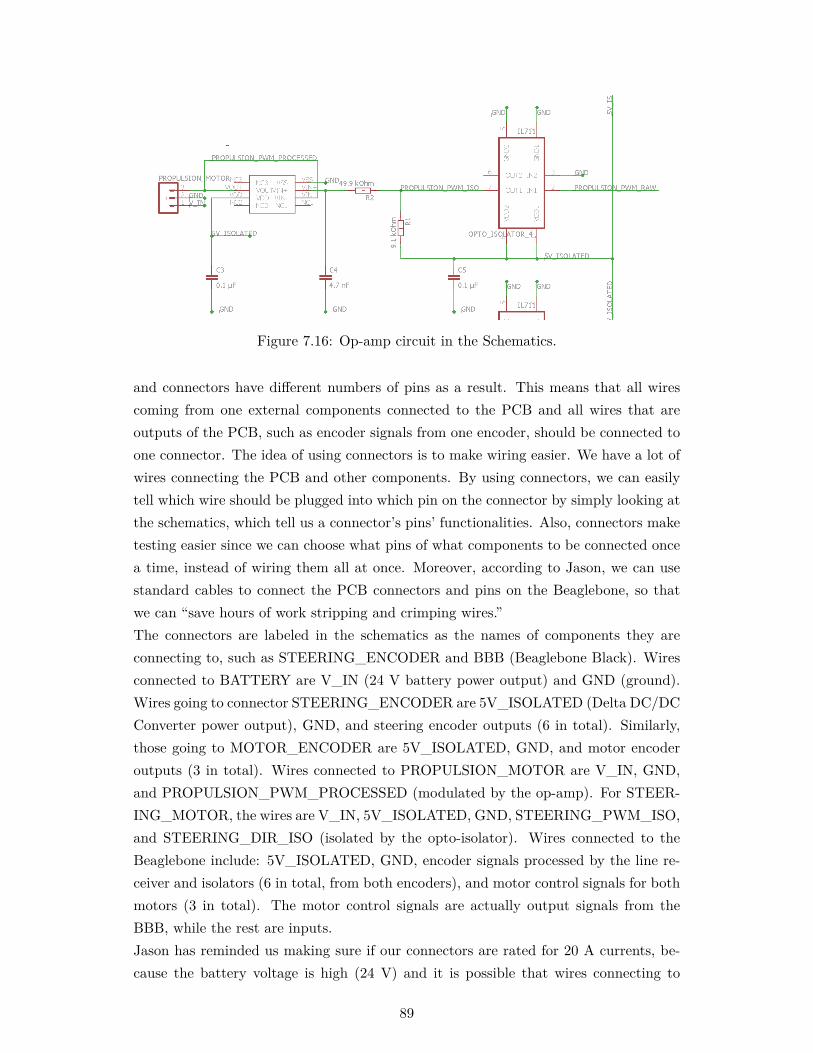
Figure 7.16: Op-amp circuit in the Schematics.
and connectors have different numbers of pins as a result. This means that all wires
coming from one external components connected to the PCB and all wires that are
outputs of the PCB, such as encoder signals from one encoder, should be connected to
one connector. The idea of using connectors is to make wiring easier. We have a lot of
wires connecting the PCB and other components. By using connectors, we can easily
tell which wire should be plugged into which pin on the connector by simply looking at
the schematics, which tell us a connector’s pins’ functionalities. Also, connectors make
testing easier since we can choose what pins of what components to be connected once
a time, instead of wiring them all at once. Moreover, according to Jason, we can use
standard cables to connect the PCB connectors and pins on the Beaglebone, so that
we can “save hours of work stripping and crimping wires.”
The connectors are labeled in the schematics as the names of components they are
connecting to, such as STEERING_ENCODER and BBB (Beaglebone Black). Wires
connected to BATTERY are V_IN (24 V battery power output) and GND (ground).
Wires going to connector STEERING_ENCODER are 5V_ISOLATED (Delta DC/DC
Converter power output), GND, and steering encoder outputs (6 in total). Similarly,
those going to MOTOR_ENCODER are 5V_ISOLATED, GND, and motor encoder
outputs (3 in total). Wires connected to PROPULSION_MOTOR are V_IN, GND,
and PROPULSION_PWM_PROCESSED (modulated by the op-amp). For STEER-
ING_MOTOR, the wires are V_IN, 5V_ISOLATED, GND, STEERING_PWM_ISO,
and STEERING_DIR_ISO (isolated by the opto-isolator). Wires connected to the
Beaglebone include: 5V_ISOLATED, GND, encoder signals processed by the line re-
ceiver and isolators (6 in total, from both encoders), and motor control signals for both
motors (3 in total). The motor control signals are actually output signals from the
BBB, while the rest are inputs.
Jason has reminded us making sure if our connectors are rated for 20 A currents, be-
cause the battery voltage is high (24 V) and it is possible that wires connecting to
89

Figure 7.17: The connector that’s supposed to connect to the Beaglebone Black in theSchematics.
V_IN and components such as the Pololu could convey a large current. If the con-
nector cannot handle the current, it could heat up and even burn a fire, eventually
damaging our circuit board.
7.4 Major Adjustments from Our Previous Design
After finishing the version 2 PCB design (version 1 was a draft that was finished before
the midterm report), Professor Ruina suggested me to give the design to Jason to have
a look, so that Jason could offer us some advice. Jason then gave us a lot of detailed
suggestions to make the design useful and correct. Some major adjustments that he
advised but were not discussed above include:
7.4.1 Pololu Motor Controller
The Pololu Motor Controller is able to drive the steering motor which uses 24V power
supply. The main reason that we choose the Pololu is that there are plenty of them
available in the lab, and since they work well with our steering motor, we don’t have
to purchase new models.
The Pololu takes two control signal inputs (PWMH and DIR), the battery 24V power
supply for the motor, and the 5V isolated power supply for the controller. Its outputs
are OUTA and OUTB, which are control signals transmitted to the motor.
90

After looking at our design, Jason suggested us to remove the Pololu from the circuit
board, because it takes a high voltage power input and a big current could be passing
it. If we were installing the Pololu on the PCB, we need to make sure first that wires
in the PCB could tolerant the large current, thus increasing difficulties of designing
the board. After thinking about this problem, we decided to exclude the Pololu from
the PCB. We are still using it, of course, but it is not a part of the PCB anymore.
The connector that we initially designed to transfer signals to the steering motor would
transfer signals to the Pololu instead, so that the Pololu could transfer the processed
control signals to the steering motor. Removing the Pololu motor controller actually
brings another benefit to our design: making the size of the circuit board smaller. A
smaller PCB could actually cost less for manufacturing. Additionally, based on the
design of the Pololu’s PCB, if we were installing it in our PCB, holes have to be drilled
on the PCB, increasing manufacturing cost as well as design and installing difficulties.
Therefore, we decided not having the Pololu in the PCB design.
7.4.2 Decoupling Capacitors
After presenting the version 2 design of the circuit board to Jason, he pointed out that
we did not include decoupling capacitors in our design. Adding decoupling capacitors
to the circuit board could help us reduce the noises created by electronic components.
Just like the long wires, electronic components installed on the circuit could produce
electromagnetic field, which generates harmful noises and could influence nearby com-
ponents. To solve this problem, we can simply add a capacitor in parallel to each
component’s power supply wire.
The capacitance of a decoupling capacitor should usually be 0.1 µF (micro-farad) or 1
µF, according to Jason. We will use capacitors available in the lab.
91

Appendix A
Example Appendix
Appendices are usually labelled with letters separate to ordinary chapters.
92

Bibliography
93