Embed Size (px)
Citation preview

Automation & Robotics Research Institute The University of Texas at Arlington
F.L. LewisMoncrief-O’Donnell Endowed Chair
Head, Controls & Sensors Group
Talk available online athttp://ARRI.uta.edu/acs
Wireless Sensor Networks

Invited by I-Ming Chen
Wireless Sensor Networks2006 Conferences on Cybernetics & Intelligent Systems (CIS)
and Robotics, Automation, & Mechatronics (RAM)
Bangkok
K.C. TanAbdullah Al Mamun
IEEE Thailand Section
Ivan Boo
First CIS-RAM Singapore 2004IEEE SMC ChapterIEEE R&A ChapterNUS / NTU / SIMTECH
Sam GeK.C. TanDanwei Wangand team
2008 ?

Papers Due 15 Nov

Bhumibol Adulyadej- Rama IX, 1946
SILVER JUBILEE – 60 years

Kingdoms of Thailand
454 Emerald Buddha found in Chiang Rai1279 Sukhotai Kingdom1351 Ayutthaya Kingdom - U Thong1767 Thonburi – Taksin
Emerald Buddha brought to Bangkok1782 Bangkok – Chakri – Rama I1868 Chulalongkorn – Rama V1946 Bhumibol Adulyadej – Rama IX
PDA
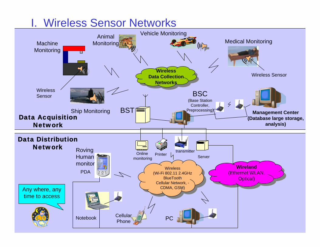
BSC(Base Station
Controller, Preprocessing)BST
WirelessSensor
Machine Monitoring
Medical Monitoring
Wireless SensorWireless
Data Collection Networks
Wireless(Wi-Fi 802.11 2.4GHz
BlueToothCellular Network, -
CDMA, GSM)
Printer
Wireland(Ethernet WLAN,
Optical)
Animal Monitoring
Vehicle Monitoring
Onlinemonitoring Server
transmitter
Any where, any time to access
Notebook Cellular Phone PC
Ship Monitoring
I. Wireless Sensor Networks
RovingHumanmonitor
Data Distribution Network
Management Center(Database large storage,
analysis)Data Acquisition
Network
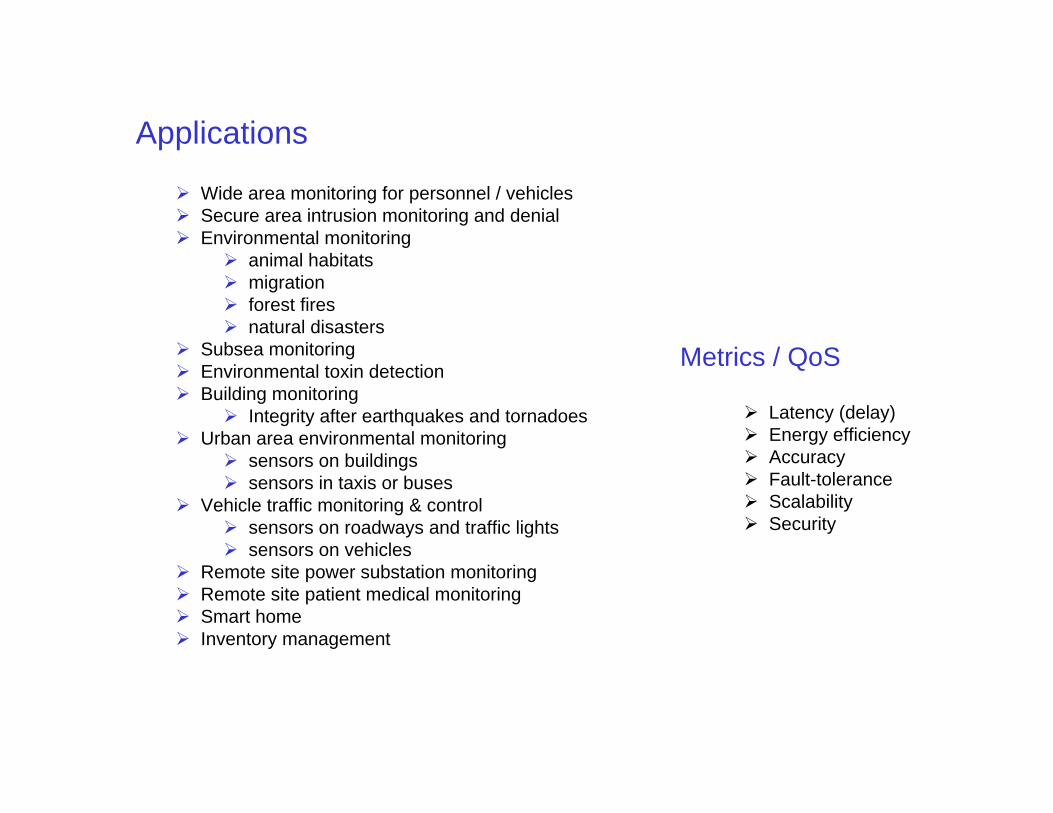
Applications
Wide area monitoring for personnel / vehiclesSecure area intrusion monitoring and denialEnvironmental monitoring
animal habitatsmigrationforest firesnatural disasters
Subsea monitoringEnvironmental toxin detectionBuilding monitoring
Integrity after earthquakes and tornadoesUrban area environmental monitoring
sensors on buildingssensors in taxis or buses
Vehicle traffic monitoring & controlsensors on roadways and traffic lightssensors on vehicles
Remote site power substation monitoringRemote site patient medical monitoringSmart homeInventory management
Latency (delay)Energy efficiencyAccuracyFault-toleranceScalabilitySecurity
Metrics / QoS
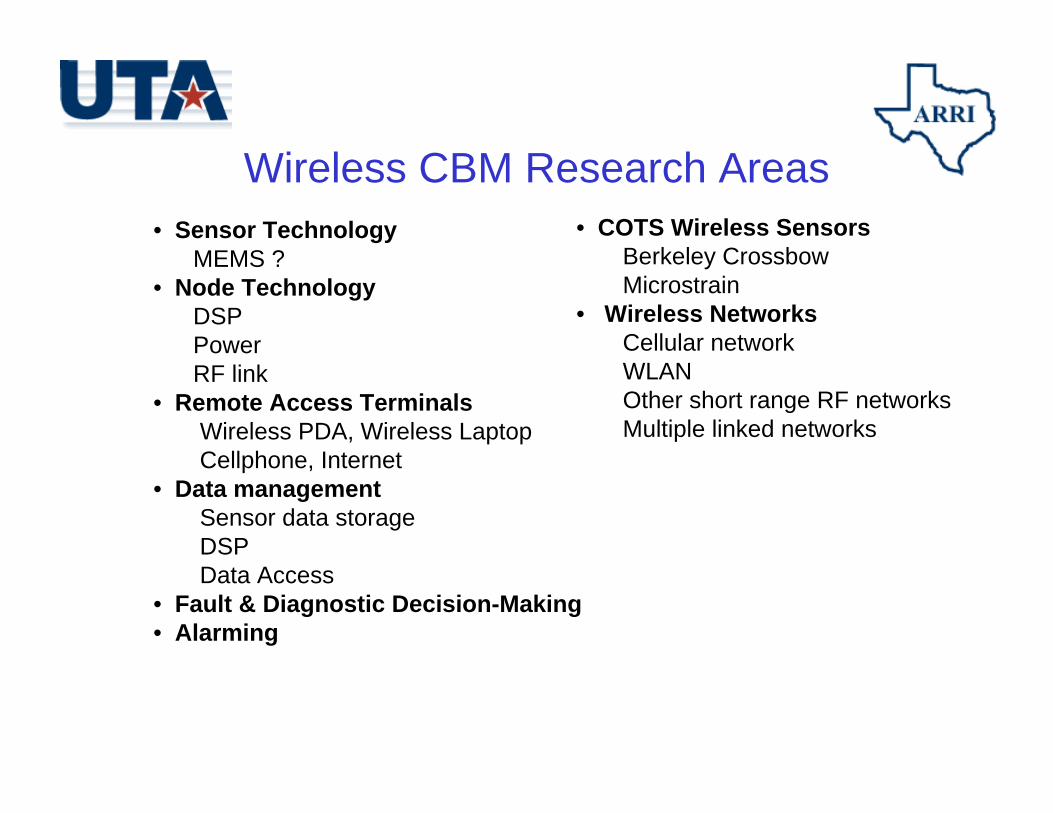
• COTS Wireless SensorsBerkeley CrossbowMicrostrain
• Wireless NetworksCellular networkWLANOther short range RF networksMultiple linked networks
Wireless CBM Research Areas• Sensor Technology
MEMS ?• Node Technology
DSPPowerRF link
• Remote Access TerminalsWireless PDA, Wireless LaptopCellphone, Internet
• Data managementSensor data storageDSPData Access
• Fault & Diagnostic Decision-Making• Alarming
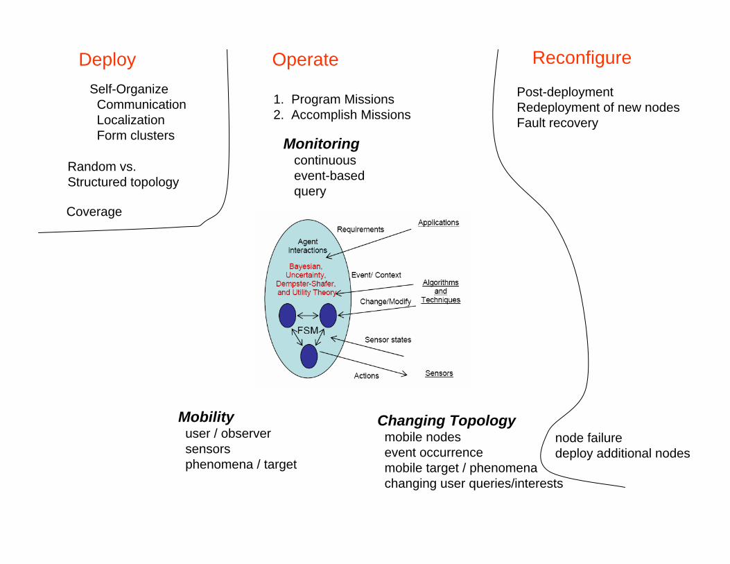
Self-OrganizeCommunicationLocalizationForm clusters Monitoring
continuousevent-basedquery
Random vs. Structured topology
Post-deploymentRedeployment of new nodesFault recovery
Deploy Operate Reconfigure
1. Program Missions2. Accomplish Missions
Mobilityuser / observersensorsphenomena / target
Changing Topologymobile nodesevent occurrencemobile target / phenomenachanging user queries/interests
node failuredeploy additional nodes
Coverage

Research TopicsDeploy
Self-organizationComms. wakeupLocalization
Sensing
Event detectionInterpret data
Responsive actionUser broadcast interestRespond to queries
CooperationDynamic Clustering
CommunicationsDynamically reconfigurableEvent-based routing
Data TransmissionEvent-basedData aggregationSensor Data fusionInformation fusionDecision fusion
Fault tolerancenode failurelink failure
Security
Programmable WSNProgram missions quickly
Task schedulingDynamic resource assignment
Scalability- NP complexityDistributed local algorithms vs. global
Meet QoS requirementsCommunicationsSensing High priority data
Decision-making & control
Use Mobility toLocalize nodesMaintain connectivityOptimize comms.Optimize sensor coverageReduce measurement uncertainty Lack of testbeds
Energy conservation
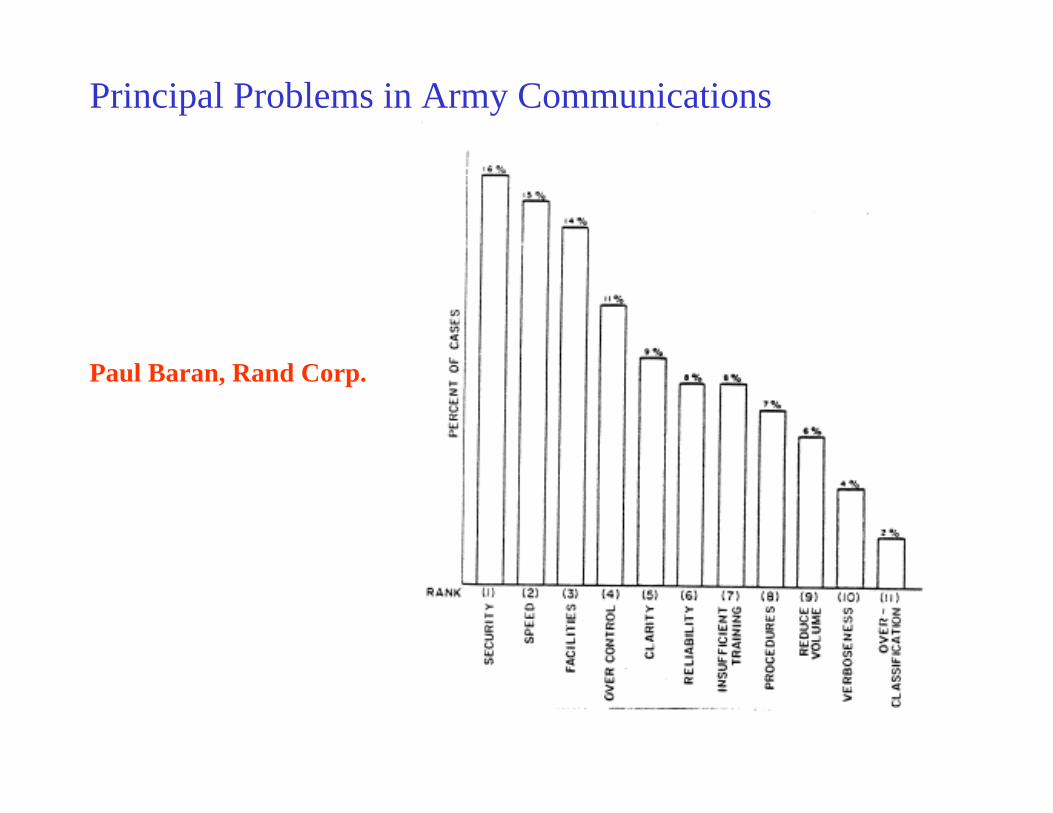
Principal Problems in Army Communications
Paul Baran, Rand Corp.
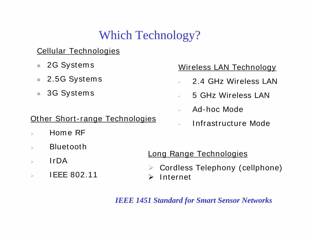
Cellular Technologies
2G Systems
2.5G Systems
3G Systems
Other Short-range Technologies
Home RF
Bluetooth
IrDA
IEEE 802.11
Wireless LAN Technology
• 2.4 GHz Wireless LAN
• 5 GHz Wireless LAN
• Ad-hoc Mode
• Infrastructure Mode
Which Technology?
IEEE 1451 Standard for Smart Sensor Networks
Long Range Technologies
Cordless Telephony (cellphone)Internet
Frequency Bands for WSN
The Industrial, Scientific and medical (ISM) radio bands were originallyreserved internationally for non-commercial use of RF EM fields forindustrial, scientific and medical purposes. In recent years they have beenused for license free communications applications such as sensor networksand bluetooth.
The bands generally used for WSN in ISM are:
433MHz933 MHz2.4 GHz5.8 GHz
http://www.pctechguide.com/29network.htm
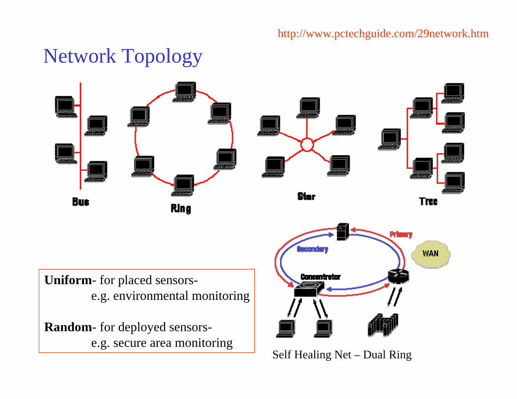
Network Topology
Self Healing Net – Dual Ring
Uniform- for placed sensors-e.g. environmental monitoring
Random- for deployed sensors-e.g. secure area monitoring

Paul Baran, Rand Corp.The Spider Web Net

Paul Baran, Rand Corp.
Centralized, Decentralized, Distributed
Neighbor Connectivity and RedundancyNetwork Topology

Paul Baran, Rand Corp.Connectivity and Number of Links
Number of links increases exponentially

The Problem of Complexity
Communication Protocols in a network must be restricted and organized to avoid Complexity problems
e.g. in ManufacturingThe general Job Shop allows part flows between all machinesThe Flow Line allows part flows only along specific Paths
We have shown that the job shop is NP-complete
but the reentrant flow line is of polynomial complexity
Lewis, Horne, Abdallah, 2000
Think of the military chain of command

Ethernet. The Ethernet was developed in the mid 1970’s by Xerox, DEC, and Intel, and was standardized in 1979. The Institute of Electrical and Electronics Engineers (IEEE) released the official Ethernet standard IEEE 802.3 in 1983. The Fast Ethernet operates at ten times the speed of the regular Ethernet, and was officially adopted in 1995. It introduces new features such as full-duplex operation and auto-negotiation. Both these standards use IEEE 802.3 variable-length frames having between 64 and 1514-byte packets.
Token Ring. In 1984 IBM introduced the 4Mbit/s token ring network. The system was of high quality and robust, but its cost caused it to fall behind the Ethernet in popularity. IEEE standardized the token ring with the IEEE 802.5 specification. The Fiber Distributed Data Interface (FDDI) specifies a 100Mbit/s token-passing, dual-ring LAN that uses fiber optic cable. It was developed by the American National Standards Institute (ANSI) in the mid 1980s, and its speed far exceeded current capabilities of both Ethernet and IEEE 802.5.
Gigabit Ethernet. The Gigabit Ethernet Alliance was founded in 1996, and the Gigabit Ethernet standards were ratified in 1999, specifying a physical layer that uses a mixture of technologies from the original Ethernet and fiber optic cable technologies from FDDI.
Historical Development and Standards
http://www.pctechguide.com/29network.htm

Client-Server networks became popular in the late 1980’s with the replacement of large mainframe computers by networks of personal computers. Application programs for distributed computing environments are essentially divided into two parts: the client or front end, and the server or back end. The user’s PC is the client and more powerful server machines interface to the network..
Peer-to-Peer networking architectures have all machines with equivalent capabilities and responsibilities. There is no server, and computers connect to each other, usually using a bus topology, to share files, printers, Internet access, and other resources.
Peer-to-Peer Computing is a significant next evolutionary step over P2P networking. Here, computing tasks are split between multiple computers, with the result being assembled for further consumption. P2P computing has sparked a revolution for the Internet Age and has obtained considerable success in a very short time. The Napster MP3 music file sharing application went live in September 1999, and attracted more than 20 million users by mid 2000.
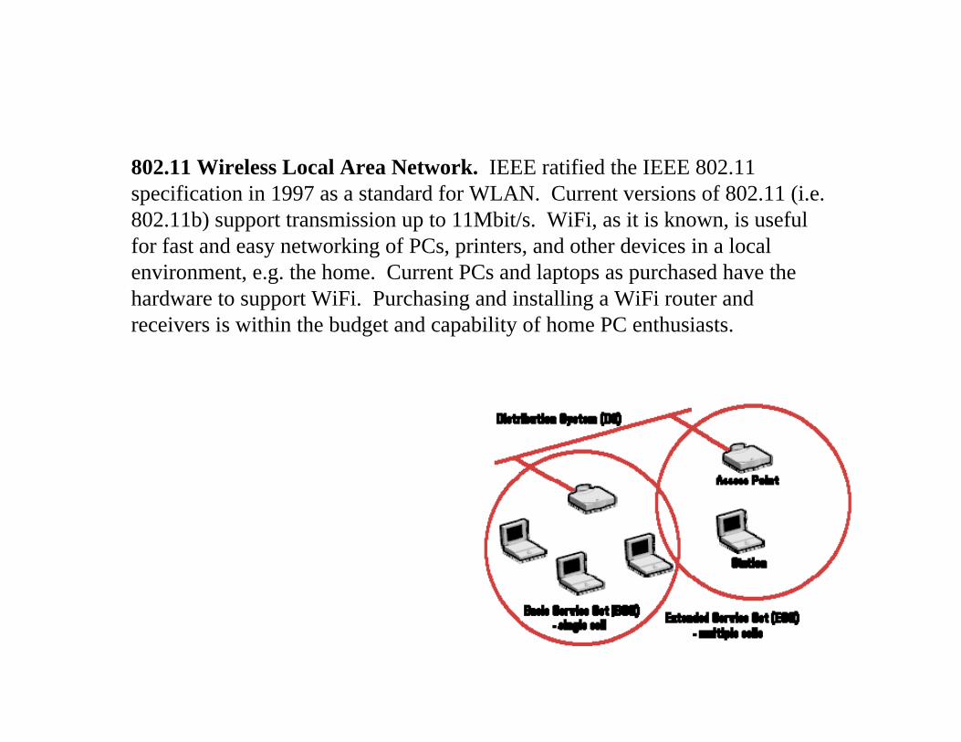
802.11 Wireless Local Area Network. IEEE ratified the IEEE 802.11 specification in 1997 as a standard for WLAN. Current versions of 802.11 (i.e. 802.11b) support transmission up to 11Mbit/s. WiFi, as it is known, is useful for fast and easy networking of PCs, printers, and other devices in a local environment, e.g. the home. Current PCs and laptops as purchased have the hardware to support WiFi. Purchasing and installing a WiFi router and receivers is within the budget and capability of home PC enthusiasts.
Bluetooth was initiated in 1998 and standardized by the IEEE as Wireless Personal Area Network (WPAN) specification IEEE 802.15. Bluetooth is a short range RF technology aimed at facilitating communication of electronic devices between each other and with the Internet, allowing for data synchronization that is transparent to the user. Supported devices include PCs, laptops, printers, joysticks, keyboards, mice, cell phones, PDAs, and consumer products. Mobile devices are also supported. Discovery protocols allow new devices to be hooked up easily to the network. Bluetooth uses the unlicensed 2.4 GHz band and can transmit data up to 1Mbit/s, can penetrate solid non-metal barriers, and has a nominal range of 10m that can be extended to 100m. A master station can service up to 7 simultaneous slave links. Forming a network of these networks, e.g. a piconet, can allow one master to service up to 200 slaves.
Currently, Bluetooth development kits can be purchased from a variety of suppliers, but the systems generally require a great deal of time, effort, and knowledge for programming and debugging. Forming piconets has not yet been streamlined and is unduly difficult.
Home RF was initiated in 1998 and has similar goals to Bluetooth for WPAN. Its goal is shared data/voice transmission. It interfaces with the Internet as well as the Public Switched Telephone Network. It uses the 2.4 GHz band and has a range of 50 m, suitable for home and yard. A maximum of 127 nodes can be accommodated in a single network. IrDA is a WPAN technology that has a short-range, narrow-transmission-angle beam suitable for aiming and selective reception of signals.
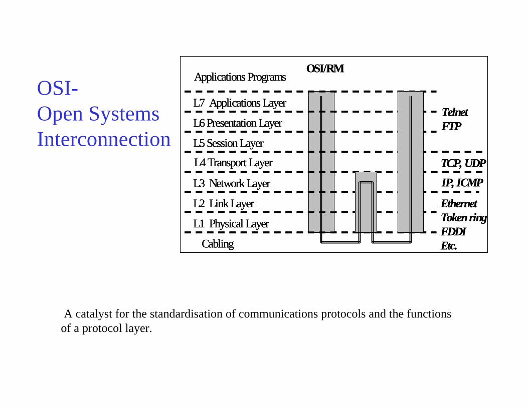
A catalyst for the standardisation of communications protocols and the functions of a protocol layer.
OSI-Open Systems Interconnection
Cabling
L1 Physical Layer
L2 Link Layer
L3 Network Layer
L4 Transport Layer
L5 Session Layer
L6 Presentation Layer
L7 Applications Layer
Applications Programs
TelnetFTP
TCP, UDP
IP, ICMP
EthernetToken ringFDDIEtc.
OSI/RM
Cabling
L1 Physical Layer
L2 Link Layer
L3 Network Layer
L4 Transport Layer
L5 Session Layer
L6 Presentation Layer
L7 Applications Layer
Applications Programs
TelnetFTP
TCP, UDP
IP, ICMP
EthernetToken ringFDDIEtc.
OSI/RM

L1 Physical Layer
L2 Link Layer
L3 Network Layer
L4 Transport Layer
L5 Session Layer
L6 Presentation Layer
L7 Applications Layer
Communicationsinfrastructure
L1 Physical Layer
L2 Link Layer
L3 Network Layer
L4 Transport Layer
L5 Session Layer
L6 Presentation Layer
L7 Applications Layer
Sensingapplication
Akyildiniz, Su, et al. 2002
Cross-layer design
ConfigureMaintainOptimize
e.g. Integrate navigation, communication, congestion control, and sensing

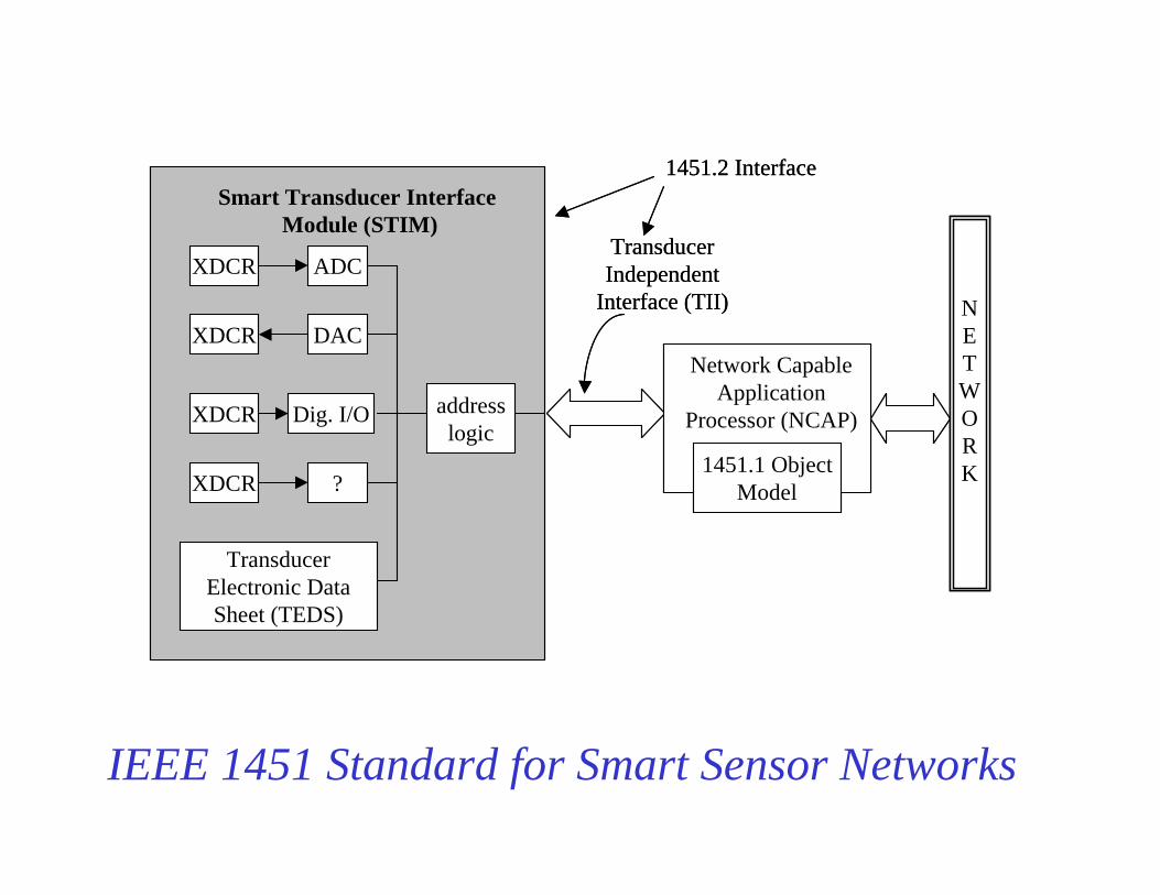
http://ieee1451.nist.gov/intro.htm
Objective of IEEE 1451 - Smart Transducer Interface Standard.To make it easier for transducer manufacturers to develop smart devices and to
interface those devices to networks, systems, and instruments by incorporating existing and emerging sensor- and networking technologies.
IEEE 1451 Standard for Smart Sensor Networks
History of IEEE-1451In September 1993, the National Institute of Standards and Technology (NIST) and the Institute of Electrical and Electronics Engineers (IEEE)'s Technical Committee on Sensor Technology of the Instrumentation and Measurement Society co-sponsored a meeting and set up four working groups -
P1451.1 Defining a common object model for smart transducers along with interface specifications for the components of the model.
P1451.2 Defining a smart transducer interface module (STIM), a transducer electronic data sheet (TEDS), and a digital interface to access the data.
P1451.3 working group aims at defining a digital communication interface for distributed multidrop systems.
P1451.4 Defining a mixed-mode communication protocol for smart transducers. The working groups created the concept of smart sensors to control networks
interoperability and to ease the connectivity of sensors and actuators into a device or field network.
sensor signalconditioning
DSP
local userinterface
applicationalgorithms
data storage
communicationanalog-to-
digitalconversion
NETWORK
hardwareinterface
Network SpecificNetwork Independent
Virtual Sensor
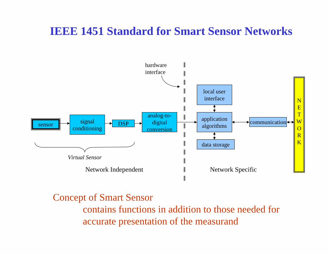
IEEE 1451 Standard for Smart Sensor Networks
Concept of Smart Sensorcontains functions in addition to those needed foraccurate presentation of the measurand
IEEE 1451 Standard for Smart Sensor Networks
XDCR ADC
XDCR DAC
XDCR Dig. I/O
XDCR ?
TransducerElectronic DataSheet (TEDS)
addresslogic
Smart Transducer Interface Module (STIM)
NETWORK
Network CapableApplication
Processor (NCAP)
1451.1 ObjectModel
TransducerIndependent
Interface (TII)
1451.2 Interface
XDCR ADC
XDCR DAC
XDCR Dig. I/O
XDCR ?
TransducerElectronic DataSheet (TEDS)
addresslogic
Smart Transducer Interface Module (STIM)
NETWORK
Network CapableApplication
Processor (NCAP)
1451.1 ObjectModel
TransducerIndependent
Interface (TII)
1451.2 Interface

Sensors &Transducers
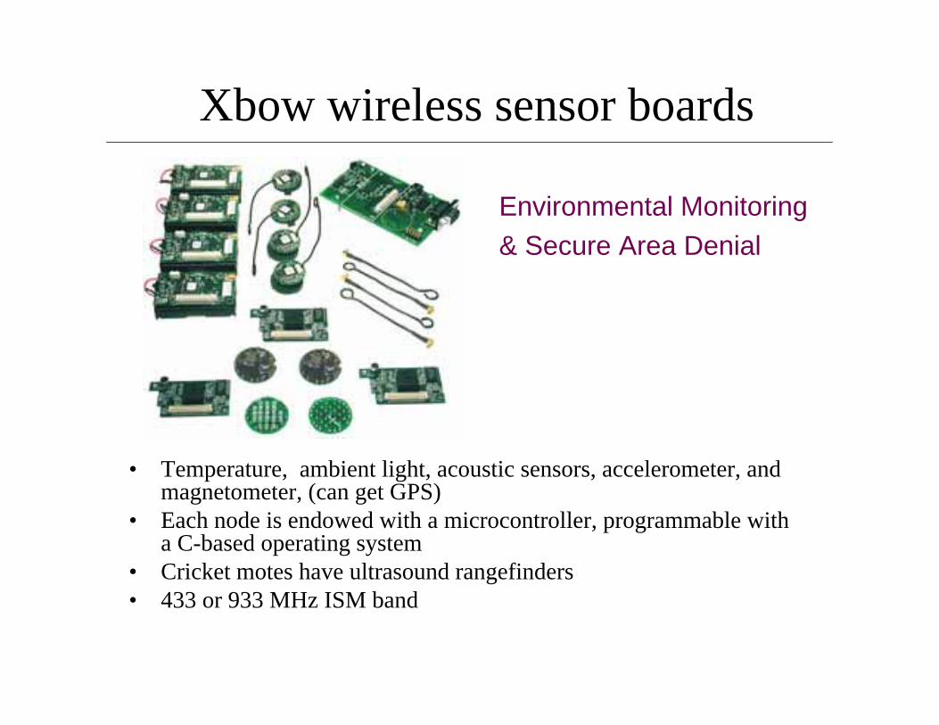
Xbow wireless sensor boards
• Temperature, ambient light, acoustic sensors, accelerometer, and magnetometer, (can get GPS)
• Each node is endowed with a microcontroller, programmable with a C-based operating system
• Cricket motes have ultrasound rangefinders• 433 or 933 MHz ISM band
Environmental Monitoring & Secure Area Denial
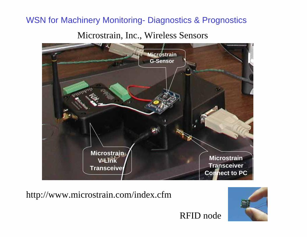
Microstrain V-Link
Transceiver
MicrostrainTransceiver
Connect to PC
MicrostrainG-Sensor
Microstrain, Inc., Wireless Sensors
RFID node
http://www.microstrain.com/index.cfm
MicrostrainG-Sensor
MicrostrainTransceiver
Connect to PC
Microstrain V-Link
Transceiver
WSN for Machinery Monitoring- Diagnostics & Prognostics

Signal ConditioningTemperature compensation
Low pass filter for noise rejection
V1 V2
R1 R2
C
V1 V2
R1 R2
CAnalog LPF
asaksH+
=)( kk szzKsα−+
=1ˆ
Digital LPF
)(ˆ 11 kkkk ssKss ++= ++ αDifference equation
Filtered velocity )( 11 kkkk ssKvv −+= ++ α
R1 R2
R3 R4
Vref
Vo
R1 R2
R3 R4
Vref
Vo
Wheatstone BridgeChanges in R converted to changes in VImproved sensitivity
DSP- Kalman Filter
kkkk AKzBuxKHIAx ++−=+ ˆ)(ˆ 1
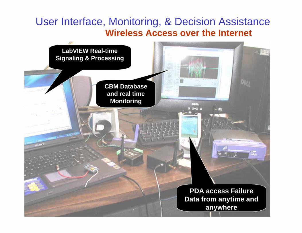
LabVIEW Real-time Signaling & Processing
CBM Database and real time Monitoring
PDA access Failure Data from anytime and
anywhere
User Interface, Monitoring, & Decision AssistanceWireless Access over the Internet
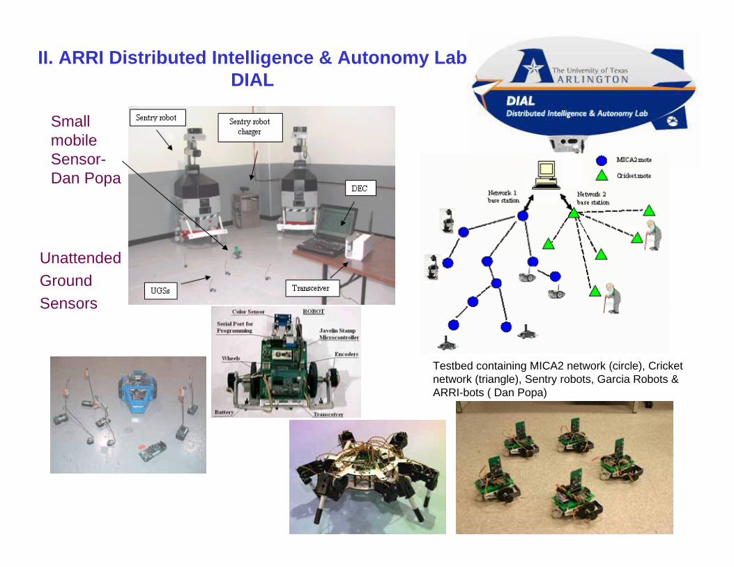
II. ARRI Distributed Intelligence & Autonomy LabDIAL
UnattendedGroundSensors
SmallmobileSensor-Dan Popa
Testbed containing MICA2 network (circle), Cricket network (triangle), Sentry robots, Garcia Robots & ARRI-bots ( Dan Popa)
!
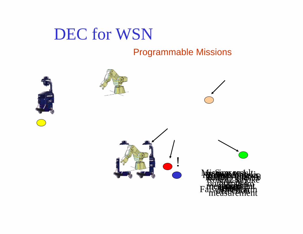
DEC for WSN
Mission result:
False fire alarmRobot1 goes to
sensor 2Sensor 1
output:alarmRobot 1 picks
sensor 2Robot2 follows
robot1Sensor 3
measurementSensor 4
measurementRobot1 places
sensor 2Sensor2
measurement
Robot1 goes to sensor1
Robot2 smoke detection
Programmable Missions

Table I- Mission1-Task sequence
Mission 1 completedy1output
S2 takes measurementS2m1Task 11
R1 takes measurementR1m1Task 10
R1 deploys UGS2R1dS21Task 9
R2 takes measurementR2m1Task 8
R1 gores to UGS1R1gS11Task 7
R1 listens for interruptsR1lis1Task 6
R1 retrieves UGS2R1rS21Task 5
R2 goes to location AR2gA1Task 4
R1 goes to UGS2R1gS21Task 3
UGS5 takes measurementS5m1Task 2
UGS4 takes measurementS4m1Task 1
UGS1 launches chemical alertu1Input 1
Descriptionnotationmission1
Table II- Mission 2-Task sequence
Mission 2 completedy2output
R1 docks the chargerR1dC2Task 5
UGS3 takes measurementS3m2Task 4
R1 charges UGS3R1cS32Task 3
R1 goes to UGS3R1g S32Task 2
UGS1 takes measurementS1m2Task 1
UGS3 batteries are lowu2input
DescriptionnotationMission2
Fast Programming of Missions
Multiple Missions
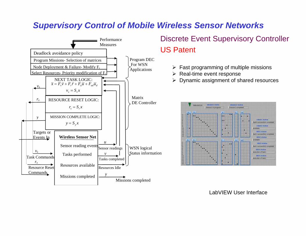
Node Deployment & Failure- Modify Fr
RESOURCE RESET LOGIC:
MISSION COMPLETE LOGIC:
Wireless Sensor Net
Sensor reading events
Tasks performed
Resources available
PerformanceMeasures
Targets or Events In
Matrix DE Controller
u
v
y
vs
rs
vs
dudurv uFuFrFvFx +++=xSv vs =
xSr rs =
xSy y=
Program DEC For WSN Applications
Program Missions- Selection of matrices
Select Resources- Priority modification of Fr NEXT TASK LOGIC:
Missions completed
Sensor readings
Tasks completed
Resources Idle
Missions completed
Task Commands
Resource Reset Commands
WSN logical Status information
y
Node Deployment & Failure- Modify Fr
RESOURCE RESET LOGIC:
xSr rs =
rs
Deadlock avoidance policy
Discrete Event Supervisory ControllerUS Patent
Supervisory Control of Mobile Wireless Sensor Networks
LabVIEW User Interface
Fast programming of multiple missionsReal-time event responseDynamic assignment of shared resources

NetEntry-inviteresponseponter
StartupNodeID nr.
Neighborinfo
I R P
Dist.toNeigh-bors
Comm link mesh info Position grid info
(x,y) coords.and OriginNode ID
Hier.routingnr.
extra
T frame
repeat nextTDMA frame
NetEntry-inviteresponseponter
StartupNodeID nr.
Neighborinfo
I R P
Dist.toNeigh-bors
Comm link mesh info Position grid info
(x,y) coords.and OriginNode ID
Hier.routingnr.
extra
T frame
repeat nextTDMA frame
TDMA frame for both communication protocols and relative positioning
Node Relative Positioning & LocalizationAd hoc network- scattered nodes
Nodes must self organize
Calibrated network-Each node knows its relative position

1 2d12 x
a. Two nodes- define x & y axes
y
b. 3 node closed kinematic chain-compute (x3, y3)
O 1 2d12 x
d23d13
3
y
x3
y3
θ213 θx23O1 2d12 x1 2d12 x
a. Two nodes- define x & y axes
y
b. 3 node closed kinematic chain-compute (x3, y3)
O 1 2d12 x
d23d13
3
y
x3
y3
θ213 θx23O 1 2d12 x
d23d13
3
y
x3
y3
θ213 θx23O
Integrating new nodes into relative positioning grid
1 2A12 x’
A23
A13
3
y’
O’
x
y
O
TOO’
A14
A34
A24
4
1 2A12 x’
A23
A13
3
y’
O’
x
y
O
TOO’
A14
A34
A24
4
Recursive closed-kinematic chain procedure for integrating new nodes
⎥⎦
⎤⎢⎣
⎡=
10ii
i
pRA
One can write the relative location in frame O of the new point 3 in two ways. The triangle shown in the figure is a closed kinematic chain of the sort studied in [Liu and Lewis 1993, 1994]. The solution is obtained by requiring that the two maps T13and T123 be exact at point 3.
Kinematicstransformation
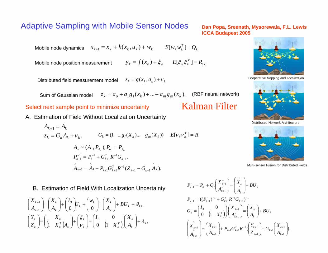
Adaptive Sampling with Mobile Sensor Nodes Dan Popa, Sreenath, Mysorewala, F.L. LewisICCA Budapest 2005
kkkkk wuxhxx ++=+ ),(1
kkk xfy ξ+= )(
kkkk axgz ν+= ),(
kTkk QwwE =][
kTkk RE 1][ =ξξ
).(...)(11 kmmkok xgaxgaaz +++=
Mobile node dynamics
Mobile node position measurement
Distributed field measurement model
Sum of Gaussian model (RBF neural network)
,1
kkkk
kk
AGzAA
ν+==+
))()...(...1( kmkik XgXgG = RE Tkk =][ νν
).(
,
),,(~
^
111
11
^
1
^1
11
111
_
0
kkkTkkkk
kTkkk
AoAoo
AGZRGPAA
GRGPP
PPPAAo
++−
+++
+−
+−−
+
−+=
+=
=
A. Estimation of Field Without Localization Uncertainty
B. Estimation of Field With Localization Uncertainty
( ) ( ) ,10
01
,00
3
3
1
1
kk
kTkk
k
kTk
k
k
k
kkk
kkk
k
k
k
k
AX
XI
AXX
ZY
BUAXw
UI
AX
AX
λνξ
ϑ
+⎟⎟⎠
⎞⎜⎜⎝
⎛⎟⎟⎠
⎞⎜⎜⎝
⎛=⎟⎟
⎠
⎞⎜⎜⎝
⎛+⎟⎟
⎠
⎞⎜⎜⎝
⎛=⎟⎟
⎠
⎞⎜⎜⎝
⎛
++⎟⎟⎠
⎞⎜⎜⎝
⎛=⎟⎟
⎠
⎞⎜⎜⎝
⎛+⎟⎟
⎠
⎞⎜⎜⎝
⎛+⎟⎟
⎠
⎞⎜⎜⎝
⎛=⎟⎟
⎠
⎞⎜⎜⎝
⎛
+
+
( )
).(
,10
0
))((
,
1
11
1
1111
1
1^
1
^
1
1
13
11
11
111
^
^
1
11
⎟⎟⎠
⎞⎜⎜⎝
⎛−⎟⎟
⎠
⎞⎜⎜⎝
⎛+⎟⎟
⎠
⎞⎜⎜⎝
⎛=⎟
⎟
⎠
⎞
⎜⎜
⎝
⎛
+⎟⎟⎠
⎞⎜⎜⎝
⎛=⎟⎟
⎠
⎞⎜⎜⎝
⎛⎟⎟⎠
⎞⎜⎜⎝
⎛=
+=
+⎟⎟
⎠
⎞
⎜⎜
⎝
⎛=⎟⎟
⎠
⎞⎜⎜⎝
⎛+=
−+
−+
+−+
+−++−
+
−+
+
+
−+
−+
−+
−+
−−++
−+
−+−
+
k
kk
k
kTkk
k
k
k
k
kk
k
k
kTk
k
kTkkk
k
k
k
k
kkk
AX
GZY
RGPAX
A
X
BUAX
AX
XI
G
GRGPP
BUA
XAX
QPP
Cooperative Mapping and Localization
Distributed Network Architecture
Multi-sensor Fusion for Distributed Fields
Select next sample point to minimize uncertainty Kalman Filter
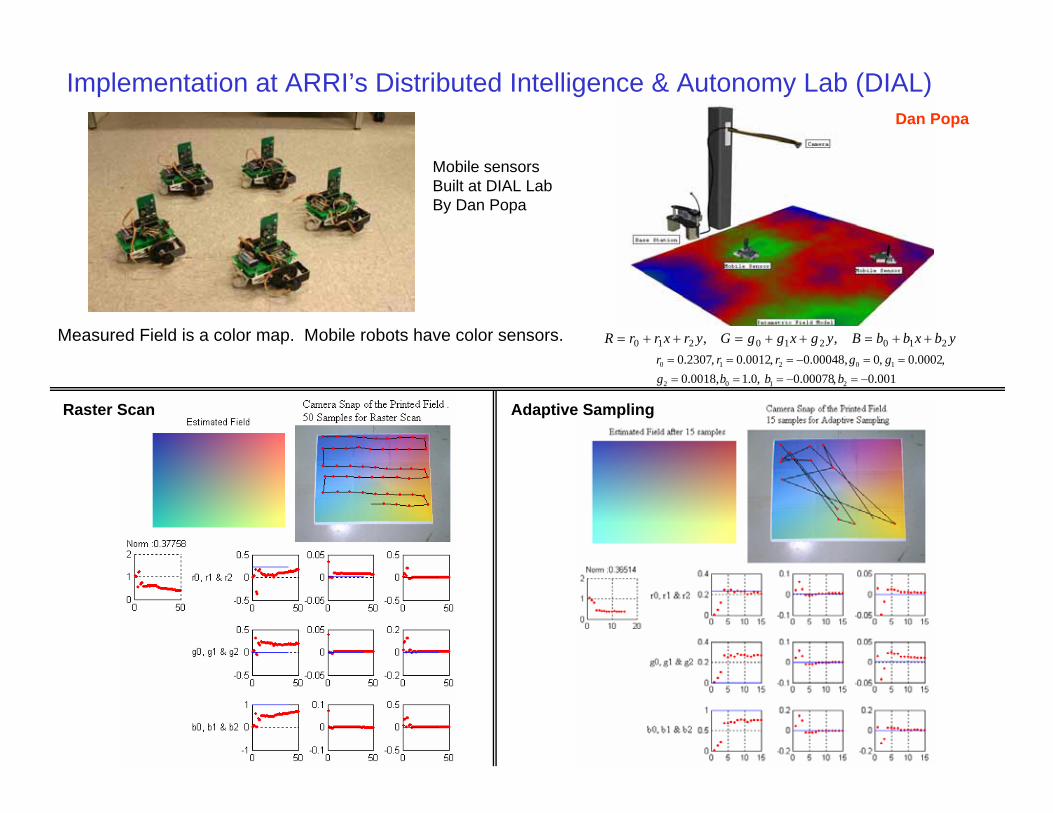
Implementation at ARRI’s Distributed Intelligence & Autonomy Lab (DIAL)
Measured Field is a color map. Mobile robots have color sensors. ybxbbBygxggGyrxrrR 210210210 ,, ++=++=++=
0.001,0.00078,0.10.0018,,0.0002,00.00048,,0.0012,0.2307
2102
10210
−=−=====−===
bbbgggrrr
Mobile sensorsBuilt at DIAL LabBy Dan Popa
Raster Scan Adaptive Sampling
Dan Popa
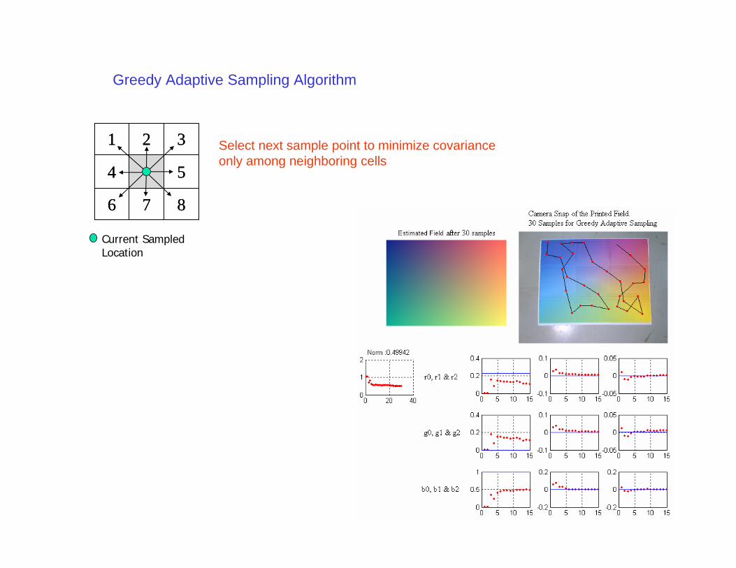
Greedy Adaptive Sampling Algorithm
876
54
321
876
54
321
Current Sampled Location
Select next sample point to minimize covarianceonly among neighboring cells

Cross-Layer Navigation Using Potential Fields Dan Popa
)(rU r−∇=F attractive forces to the goals, repulsive forces among the robots and obstacles
)(),( ijijrestore uji rrF −= Restoring force to avoid getting out of communication range
iiiii vm Frr =+ &&& Mobile node eqs. of motion
⎟⎟⎠
⎞⎜⎜⎝
⎛+= αd
PWN
KWC t
o
1log2Shannon Link communication capacity
with internode distance d
rrPk
∂∂
−=||))((||
infF )(rPk is the adaptive sampling error covariance calculated via the EKF
∫=+=t
o
iiiiioi dtEtEkt τττνν ν )()()()),(1()( rF & Conserve energy by making damping increase withmotion energy expended
Information potential
)ˆ()ˆ(ˆ111 kk
Tkkk XXWXXM −−= −
+−++ Work to go to next predicted state for adaptive sampling
CFc −∇=
Energy cons.
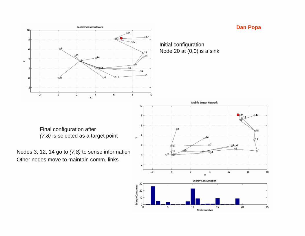
Initial configurationNode 20 at (0,0) is a sink
Final configuration after(7,8) is selected as a target point
Nodes 3, 12, 14 go to (7,8) to sense informationOther nodes move to maintain comm. links
Dan Popa

Dynamic Localization of Mobile WSN Dang, F. Lewis, D. Popa
[ ]Tiii yxX =
⎥⎥⎦
⎤
⎢⎢⎣
⎡⎥⎦
⎤⎢⎣
⎡+⎥
⎦
⎤⎢⎣
⎡⎥⎦
⎤⎢⎣
⎡=⎥
⎦
⎤⎢⎣
⎡y
i
xi
i
i
i
i
ff
IO
XX
OOIO
XX
2
2
22
22&&&
&
Node position
Estimator for position
∑∑=
≠=
−=N
i
N
jij
ijijijugs rrKV1 1
2)(21
iv
N
j ji
jiijijiji XK
XX
XXrrKf &
r−
−
−−−= ∑
=1
)()(
∑=
+=N
ii
Tiugs XXVL
1 21 &&
Potential fn.
Theorem. Let virtual force be given by
Then the position estimates reach steady-state values that provide optimal estimates of the actual relative localization of the nodes in the sense that is minimized
Proof:
1. Relative Localization
mpX aip
,...,2,1; =
∑∑∑== =
+−=m
p
ai
ai
m
p
N
j
aji
aji
ajiuav ppppp
eKrrKV1
2
1 1
2
21)(
21 [ ] 2
122 )()( a
ia
ia
ia
ia
i pppppyxxxe −+−=
∑ ∑
∑∑∑
+= =
= ==
−+
−+=
N
mp
N
jjijiji
m
p
N
j
aji
aji
aji
m
p
ai
aip
ppp
ppppp
rrK
rrKeKV
1 1
2
1 1
2
1
2
)(21
)(21
21
p
p
p
pppp iv
N
j ji
jijijijii XK
XX
XXrrKf &−
−
−−=∑
=1
)()(
ai
av
N
j ja
i
ja
iaji
aji
aji
ai
ai
ai
ai p
p
p
pppppppXK
XX
XXrrKXXKf &−
−
−−−−−= ∑
=1
)()()(
2. Absolute Localizationm nodes with GPS
abs. loc. pot. fn. with
Theorem. Let virtual force be given by
nodes with no GPS
nodes with GPS
Proof:
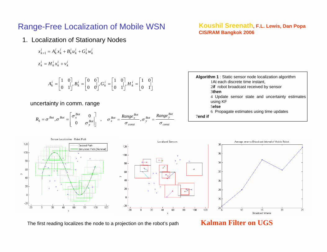
Range-Free Localization of Mobile WSN Koushil Sreenath, F.L. Lewis, Dan PopaCIS/RAM Bangkok 2006
ik
ik
ik
ik
ik
ik
ik wGuBxAx ++=+1
ik
ik
ik
ik vxHz +=
⎥⎦
⎤⎢⎣
⎡=⎥
⎦
⎤⎢⎣
⎡=⎥
⎦
⎤⎢⎣
⎡=⎥
⎦
⎤⎢⎣
⎡=
1001
,1001
,0000
,1001 i
kik
ik
ik HGBA
,0
0,
⎥⎥⎦
⎤
⎢⎢⎣
⎡== Bot
y
BotxBotBot
kRσ
σσσ
const
BotyBot
yconst
BotxBot
xRangeRangeσ
σσ
σ == ,
Algorithm 1 : Static sensor node localization algorithm1At each discrete time instant,2if robot broadcast received by sensor3then4 Update sensor state and uncertainty estimates using KF5else6 Propagate estimates using time updates
7end if
1. Localization of Stationary Nodes
uncertainty in comm. range
The first reading localizes the node to a projection on the robot’s path Kalman Filter on UGS
( ) ( )wtGtuXaX += ,,&
[ ] gpskk
gpsgpsk vktXhZ += ),(
( ) ( )⎥⎥⎥⎥
⎦
⎤
⎢⎢⎢⎢
⎣
⎡
=
⎥⎥⎥⎥⎥
⎦
⎤
⎢⎢⎢⎢⎢
⎣
⎡
=
⎥⎥⎥⎥
⎦
⎤
⎢⎢⎢⎢
⎣
⎡
=
0000000000100001
,sin
sincoscoscos
, tGL
vvv
yx
tXat
t
t
αωα
φαφα
αφ&
&&
&
[ ] [ ] ⎥⎦
⎤⎢⎣
⎡=⎥
⎦
⎤⎢⎣
⎡=
yx
ktXhyx
ktXh kugs
kgps ),(,),(
const
iyi
yconst
ixi
x
iy
ixiiiugs
k
RangeRange
PR
σσ
σσ
σσ
σσ
==
⎥⎥⎦
⎤
⎢⎢⎣
⎡=⎥⎦
⎤⎢⎣⎡ +=
,
00
,22
Includes uncertainty in position and in comm. range
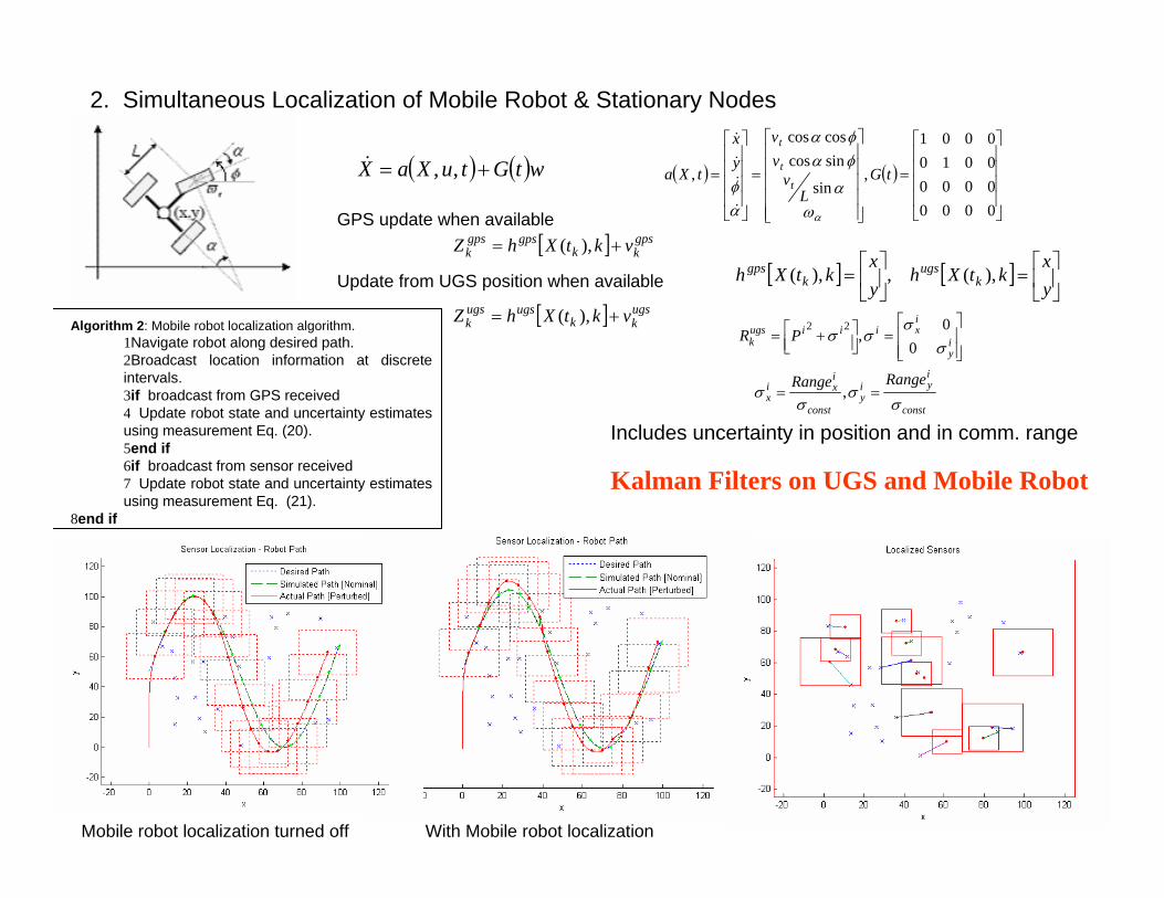
Algorithm 2: Mobile robot localization algorithm.1Navigate robot along desired path.2Broadcast location information at discrete intervals.3if broadcast from GPS received4 Update robot state and uncertainty estimates using measurement Eq. (20).5end if6if broadcast from sensor received7 Update robot state and uncertainty estimates using measurement Eq. (21).
8end if
2. Simultaneous Localization of Mobile Robot & Stationary Nodes
GPS update when available
Update from UGS position when available
[ ] ugskk
ugsugsk vktXhZ += ),(
Mobile robot localization turned off With Mobile robot localization
Kalman Filters on UGS and Mobile Robot
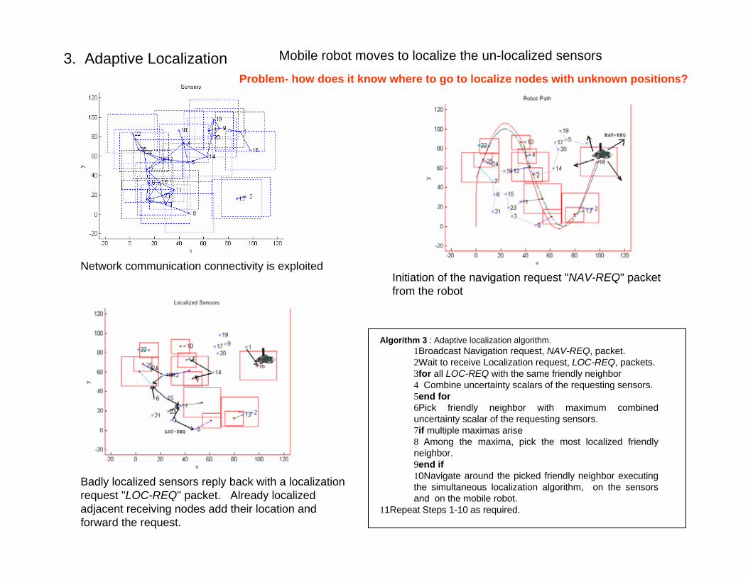
3. Adaptive Localization Mobile robot moves to localize the un-localized sensors
Network communication connectivity is exploitedInitiation of the navigation request "NAV-REQ" packet from the robot
Badly localized sensors reply back with a localization request "LOC-REQ" packet. Already localized adjacent receiving nodes add their location and forward the request.
Algorithm 3 : Adaptive localization algorithm.1Broadcast Navigation request, NAV-REQ, packet.2Wait to receive Localization request, LOC-REQ, packets.3for all LOC-REQ with the same friendly neighbor4 Combine uncertainty scalars of the requesting sensors.5end for6Pick friendly neighbor with maximum combined uncertainty scalar of the requesting sensors.7if multiple maximas arise8 Among the maxima, pick the most localized friendly neighbor.9end if10Navigate around the picked friendly neighbor executing the simultaneous localization algorithm, on the sensors and on the mobile robot.
11Repeat Steps 1-10 as required.
Problem- how does it know where to go to localize nodes with unknown positions?

Network layer
Sensor Protocols for Information via Negotiation
RoutingData fusion
SPIN protocol
Directed diffusion
Interest disseminationResponsive actionEvent detection
publish / subscribe
advertise interest
Akyildiniz, Su, et al. 2002
RoutingMinimum energyMinimum hopMax. min power available
usersensor
User/
III. Issues and Tools in WSN
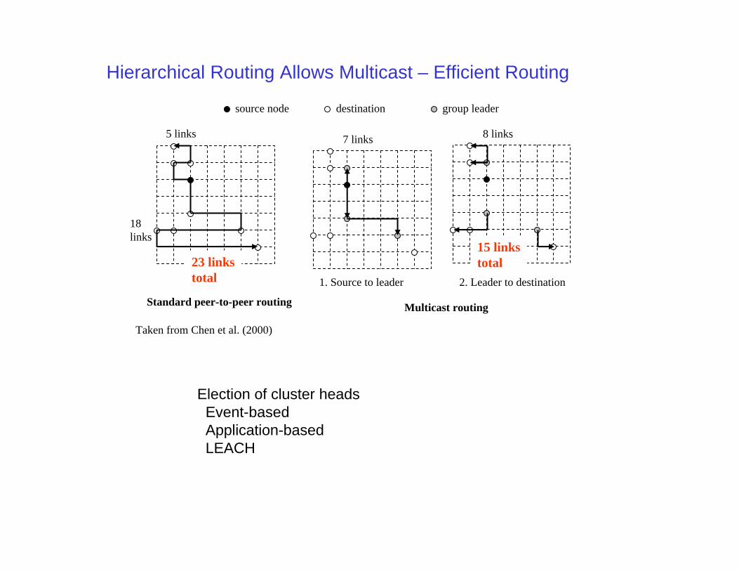
Election of cluster headsEvent-basedApplication-basedLEACH
Hierarchical Routing Allows Multicast – Efficient Routing
5 links
18links
source node destination
Standard peer-to-peer routing Multicast routing
1. Source to leader 2. Leader to destination
Taken from Chen et al. (2000)
group leader
15 linkstotal
7 links
23 linkstotal
8 links
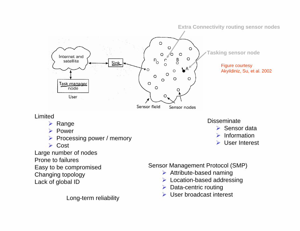
LimitedRangePowerProcessing power / memoryCost
Large number of nodesProne to failuresEasy to be compromisedChanging topologyLack of global ID
Sensor Management Protocol (SMP)Attribute-based namingLocation-based addressingData-centric routingUser broadcast interest
DisseminateSensor dataInformationUser Interest
Long-term reliability
Figure courtesyAkyildiniz, Su, et al. 2002
Tasking sensor node
Extra Connectivity routing sensor nodes

Sensor Placement and Lifetime EstimationJain and Qilian Liang, 2005
Failure of two nodes causesloss of sensor coverage
Square grid
Hex grid
Reliability TheorySurvivor Function = prob. that a unit is still functioning at time t
s(t)= 1- cdf
Reliability block diagram of square grid
32
)1)(1(1
sss
ssss cbablock
−+=
−−−=
Nblocknet ss )(=
Reliability block diagram of hex grid
)1)(1(1 3sssblock −−−=2/)( N
blocknet ss =

∑−
=ii
thresholdinitnode Pw
EET
Node lifetime
power consumed in mode i
fraction of time spent in mode i
Assume only 2 modes, then binomial pdf xTxx ppcxwP −−== )1(}{ 1
Pr node is idle
Pr node is active (defined by net protocol)
Finding node lifetime pdf
Results T= nr. of time units
Can predict net lifeMore accurately thanNode life
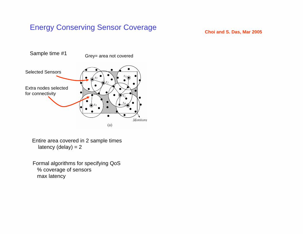
Energy Conserving Sensor Coverage
Sample time #1 Sample time #2
Selected Sensors
Extra nodes selectedfor connectivity
Selected Sensors
Extra nodes selectedfor connectivity
Grey= area not covered
Entire area covered in 2 sample timeslatency (delay) = 2
Formal algorithms for specifying QoS% coverage of sensorsmax latency
Choi and S. Das, Mar 2005
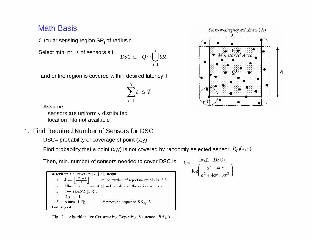
Math Basis
Select min. nr. K of sensors s.t.U
k
iiSRQDSC
1=
∩⊂
Circular sensing region SRi of radius r
and entire region is covered within desired latency T
TtN
ii ≤∑
=1Assume:
sensors are uniformly distributedlocation info not available
Find probability that a point (x,y) is not covered by randomly selected sensor ),( yxqPq
Then, min. number of sensors needed to cover DSC is
⎟⎟⎠
⎞⎜⎜⎝
⎛
+++
−=
22
2
44log
)1log(
raraara
DSCk
π
a
DSC= probability of coverage of point (x,y)1. Find Required Number of Sensors for DSC

2. Add Extra Routing Nodes for Comm. Connectivity
Test probable connectivity of k sensors in k-1 steps, adding nodes when needed
3. Construct Data Gathering Tree (DGT)For routing and sensor scheduling
Data sink sends flood messageEach sensor keeps a forwarding record
with best upstream candidateSensors broadcast join request setup msgs.
Localized sensor scheduling algorithm
Λ= /inodeofrangeradioPis
iterationnumber
Connectedset
Other nodes
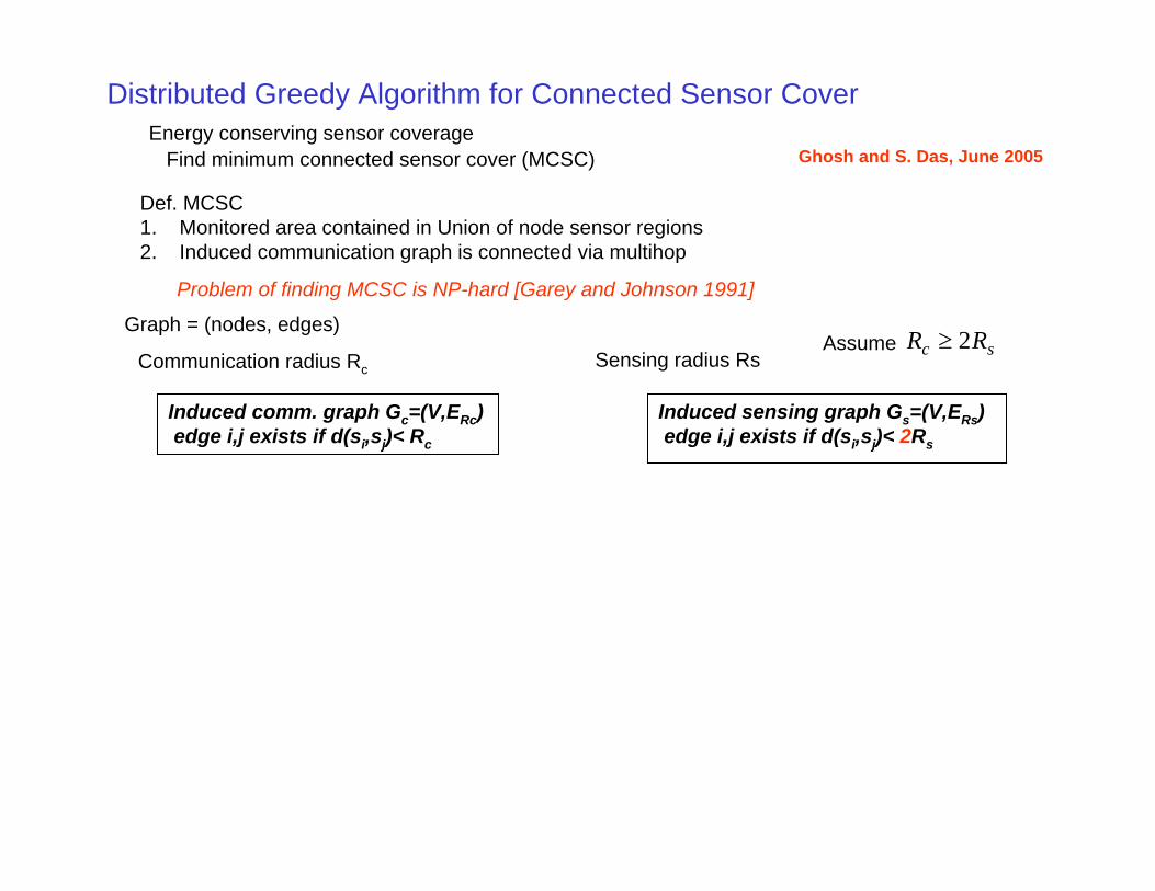
Distributed Greedy Algorithm for Connected Sensor Cover
Find minimum connected sensor cover (MCSC)
Def. MCSC1. Monitored area contained in Union of node sensor regions2. Induced communication graph is connected via multihop
Energy conserving sensor coverage
Problem of finding MCSC is NP-hard [Garey and Johnson 1991]
Ghosh and S. Das, June 2005
Communication radius Rc
Induced comm. graph Gc=(V,ERc)edge i,j exists if d(si,sj)< Rc
Induced sensing graph Gs=(V,ERs)edge i,j exists if d(si,sj)< 2Rs
Graph = (nodes, edges)
Sensing radius RsAssume sc RR 2≥

Def. Independent SetA subset of vertices such that no two vertices has an edge in G.
Def. MISAn IS that is not contained in any other IS
Finding MIS for a general graph is NP-hard
Phase 1 – Find Maximal Independent Set (MIS)

Phase 1 – Find Maximal Independent Set (MIS)
Use greedy approach looking only at 1-hop nearest neighbors
Def. Eligible next node given node si1. sj not yet included in the connected MIS2. sj a one-hop neighbor of si3. sensing circle of sj does not overlap any selected sensing circles
Suboptimal MCSC using greedy approach
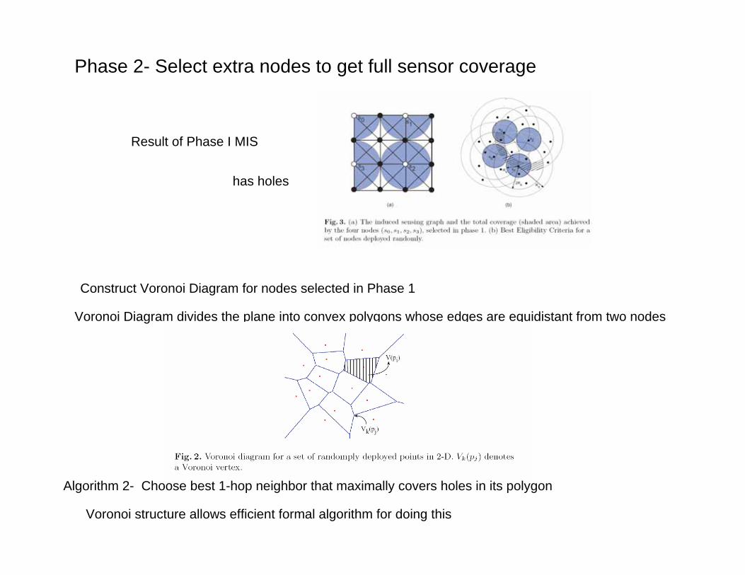
Phase 2- Select extra nodes to get full sensor coverage
Construct Voronoi Diagram for nodes selected in Phase 1
Voronoi Diagram divides the plane into convex polygons whose edges are equidistant from two nodes
Algorithm 2- Choose best 1-hop neighbor that maximally covers holes in its polygon
Voronoi structure allows efficient formal algorithm for doing this
Result of Phase I MIS
has holes
Time complexity of first algorithm is
Time complexity of second algorithm is
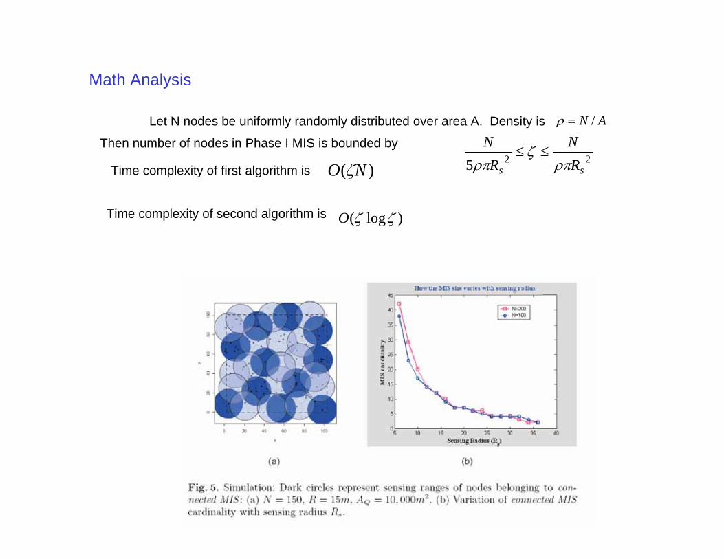
Math Analysis
Let N nodes be uniformly randomly distributed over area A. Density is
Then number of nodes in Phase I MIS is bounded by 225 ss R
NR
Nρπ
ζρπ
≤≤
AN /=ρ
)( NO ζ
)log( ζζO

Network SecurityGroup Key Distribution via Local Collaboration
Chadha, Y. Liu, and S. Das, Sept. 2005
1. (n,t) Threshold cryptography via polynomials
Random secret polynomial 1110)( −−++= t
t xaxaaxf where secret key is D= f(0)
f(x) Can be reconstructed from t points from the set {f(1), f(2), …, f(n)}, with n= number of nodes
Select masking polynomial h(x) and securely predeploy personal secrets h(i) on each node i.
The Sink broadcasts w(x)= f(x)g(x)+h(x)
Where revocation polynomial is ))...()(()( 21 wrxrxrxxg −−−=
with the set of compromised nodes },...,{ 1 wrr
Then each node i can evaluate its personal key)(
)()()(ig
ihiwif −=
Compromised nodes have g(i)=0 and cannot find personal key
Now, t nodes can collaborate to exchange personal keys f(i) and so compute f(x), and hence find the secret group key D= f(0)
Since h(i) is securely predeployed and f(x) is random, the scheme can be shown to be unconditionally secure
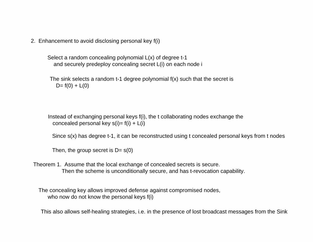
2. Enhancement to avoid disclosing personal key f(i)
Select a random concealing polynomial L(x) of degree t-1 and securely predeploy concealing secret L(i) on each node i
Instead of exchanging personal keys f(i), the t collaborating nodes exchange the concealed personal key s(i)= f(i) + L(i)
Since s(x) has degree t-1, it can be reconstructed using t concealed personal keys from t nodes
Then, the group secret is D= s(0)
The sink selects a random t-1 degree polynomial f(x) such that the secret isD= f(0) + L(0)
The concealing key allows improved defense against compromised nodes, who now do not know the personal keys f(i)
This also allows self-healing strategies, i.e. in the presence of lost broadcast messages from the Sink
Theorem 1. Assume that the local exchange of concealed secrets is secure.Then the scheme is unconditionally secure, and has t-revocation capability.
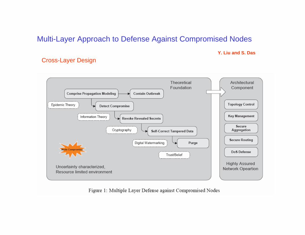
Multi-Layer Approach to Defense Against Compromised Nodes
Y. Liu and S. DasCross-Layer Design
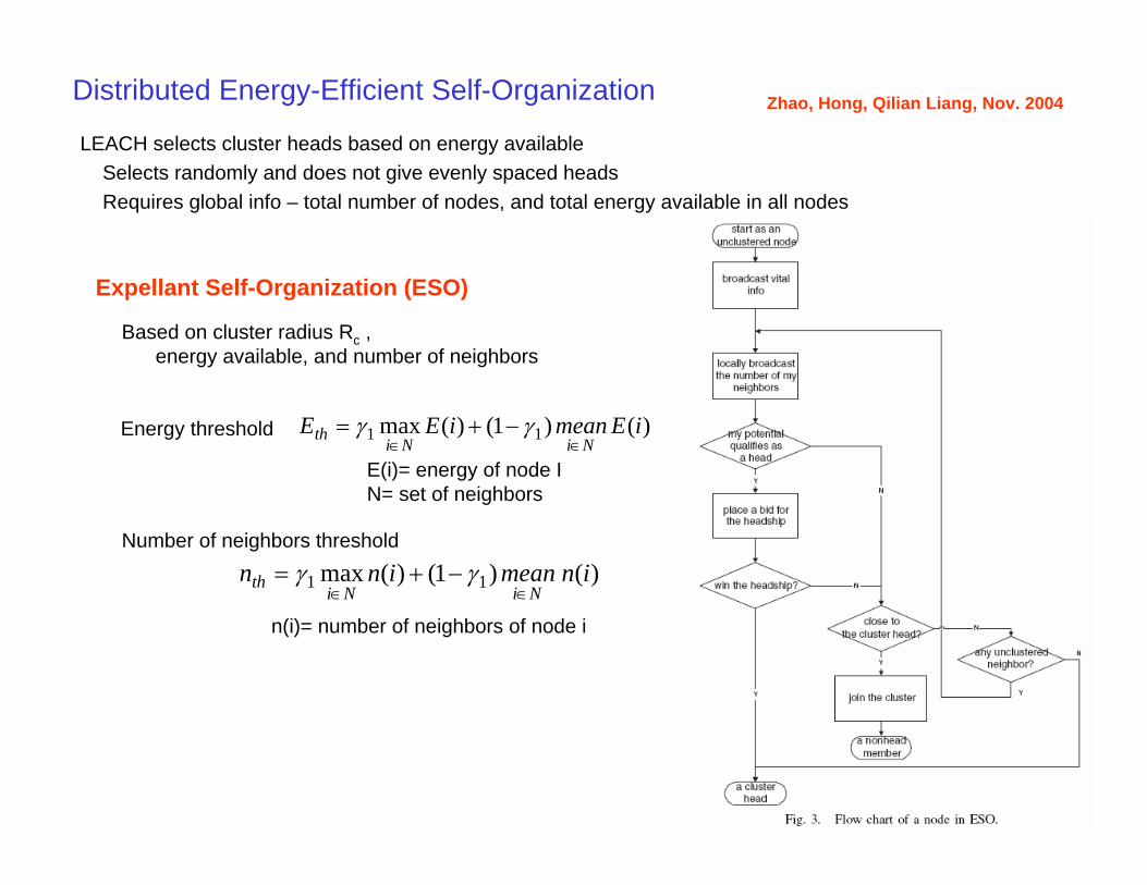
Distributed Energy-Efficient Self-Organization Zhao, Hong, Qilian Liang, Nov. 2004
LEACH selects cluster heads based on energy availableSelects randomly and does not give evenly spaced headsRequires global info – total number of nodes, and total energy available in all nodes
Expellant Self-Organization (ESO)
Based on cluster radius Rc ,energy available, and number of neighbors
)()1()(max 11 iEmeaniEENiNi
th∈∈
−+= γγ
)()1()(max 11 inmeaninnNiNi
th∈∈
−+= γγ
Energy threshold
E(i)= energy of node IN= set of neighbors
Number of neighbors threshold
n(i)= number of neighbors of node i
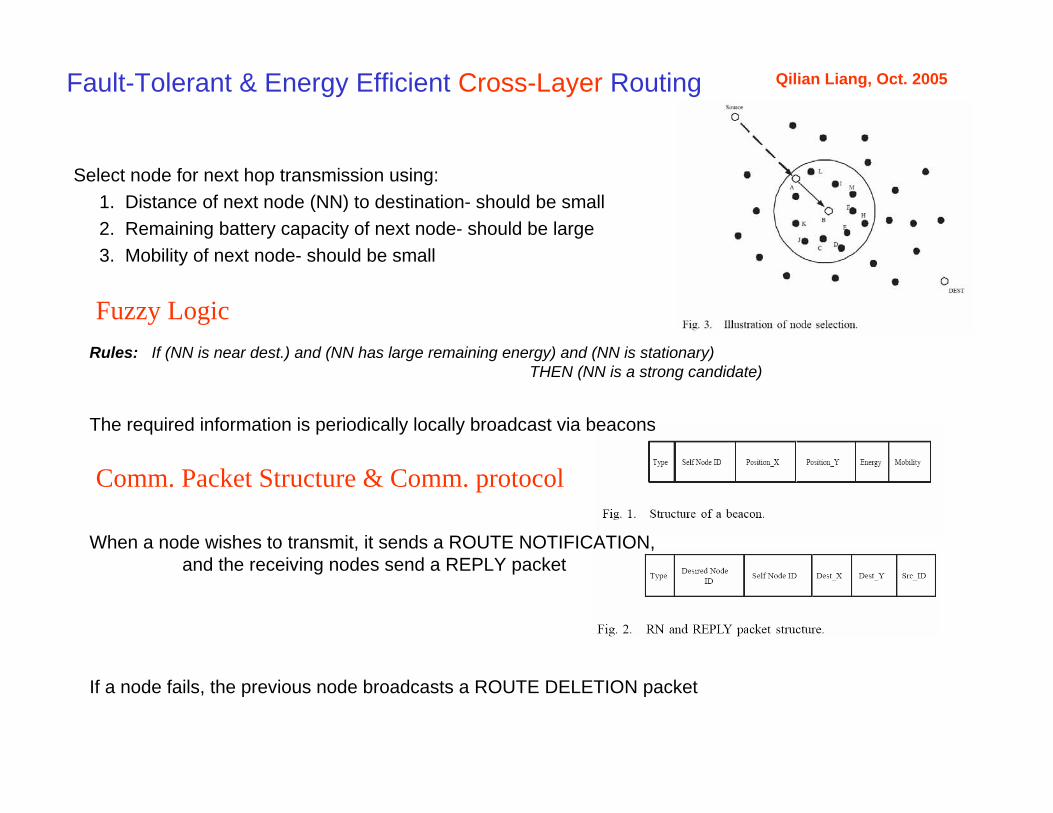
Fault-Tolerant & Energy Efficient Cross-Layer Routing Qilian Liang, Oct. 2005
Select node for next hop transmission using: 1. Distance of next node (NN) to destination- should be small 2. Remaining battery capacity of next node- should be large3. Mobility of next node- should be small
Fuzzy Logic
The required information is periodically locally broadcast via beacons
Rules: If (NN is near dest.) and (NN has large remaining energy) and (NN is stationary)THEN (NN is a strong candidate)
When a node wishes to transmit, it sends a ROUTE NOTIFICATION, and the receiving nodes send a REPLY packet
If a node fails, the previous node broadcasts a ROUTE DELETION packet
Comm. Packet Structure & Comm. protocol

Cross-Layer Routing in Sensor Networks
Luo, Yonghe Liu, Sajal Das, 2006
Transmission cost t(e)= w(e) c(e), e= an edge
Graph (nodes, edges) G= (V,E) Find Data Gathering Tree
w(e)= amount of datac(e)= transmission cost – congestion, distance, latency, energy used
Fusion cost f(e)
Fusion Cost for L bits = 2L x 5 nano Joulesthe resulting data has L(1+η) bits
re αη −−=1r = node separation, good for field measurements
Data correlation model
Maximize the cost with link cost factors given as
remaining energy at next node
(delay to reach next node) X (dist. from next node to destination )
Fonda, Zawodniok, S. Jagannathan, ISIC Munich 06
Dijkstra’s Algorithm can be used
Define cross-layer cost
Minimize the Total Cost ∑∈
+routee
etef )]()([

Transmission Costs
Transmission cost per hop 42, ≤≤∝ γγd
Total energy per packet using N hops
∑+=hops
idNE γβα
Trans. costSetup cost

Sensor / Data Fusion Luo, Lin, Scherp 1988
)}}({{),( 121 LCEfPPd =x1 x2 x
P1= P1(x/x1) P2= P2(x/x2)
)/()/()(
22
11
xxPxxPxL =
General distance measure
J-divergence
}log)1{(),( 121 LLEPPJ −=
Likelihood ratio
2/12121 })1{({),( −= LEPPd
Matsusita distance
For data representing the same property:
)1log(),( 221 dPPB −−=
Bhattacharyya’s distance
f(.) an increasing fn.C(.) a convex fn.

AdxxPxxPdj
i
x
xiiiiij 2)()/(2 == ∫
BdxxPxxPdi
j
x
xjjjjji 2)()/(2 == ∫
Distance is not symmetric
Confidence distance measures
For multiple sensors, use matrix
⎥⎥⎥⎥
⎦
⎤
⎢⎢⎢⎢
⎣
⎡
=
mmm
m
dd
ddddd
D
1
2221
11211
OM
L
Draw a digraph having edge (i,j) if
thresholddij ≤
1 2
34
Sensor 2 supportsSensor 3
Outlier-Correct or discard
Luo, Lin, Scherp 1988

Information Fusion & Sensor Selection in WSN “MIDFUSION,” Alex, Mohan Kumar, Behrooz Shirazi
Select the best set of sensors that meet the goals of the applications with guaranteed QoS
Middleware for customized services and resource assignment
Expected utility given evidence
∑=i
ninnin SGUSSGPSUE }))({(})/{})({(})({
})({ ni SG is the goal state reached as a result of the selected sensor set }{ nS
Utility of sensors can be written }{})({( nni uSGU =
Where utility factor for sensor sn is)(cost
1)1(n
nn sDu αα −+=
and Dn is a measure of the definitiveness or accuracy of sensor sn
Use Bayesian Networksgiven by user constructed by
middlewaregoal
Internal states
observables
sensors

Security Threat Example
BN showing conditional probabilities
Utility is maximized by using sensor set {RFID2, Video3}This gives 70% threshold
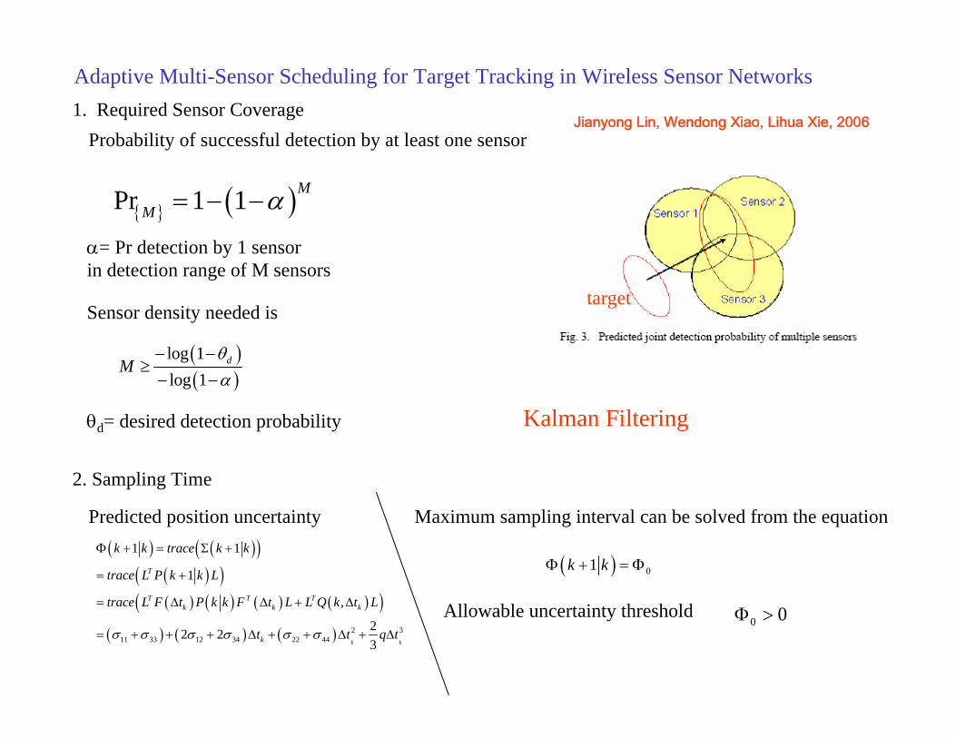
Jianyong Lin, Wendong Xiao, Lihua Xie, 2006
Adaptive Multi-Sensor Scheduling for Target Tracking in Wireless Sensor Networks
{ } ( )Pr 1 1 MM α= − −
Probability of successful detection by at least one sensor
α= Pr detection by 1 sensorin detection range of M sensors
( )( )
log 1log 1
dMθα
− −≥− −
1. Required Sensor Coverage
Sensor density needed is
θd= desired detection probability Kalman Filtering
2. Sampling Time
( ) ( )( )( )( )( ) ( ) ( ) ( )( )
( ) ( ) ( ) 2 311 33 12 34 22 44
1 1
1
,
22 23k k
T
T T Tk k k
k
k k trace k k
trace L P k k L
trace L F t P k k F t L L Q k t L
t t q tσ σ σ σ σ σ
Φ + = Σ +
= +
= Δ Δ + Δ
= + + + Δ + + Δ + Δ
Predicted position uncertainty
( ) 01k kΦ + = Φ
Maximum sampling interval can be solved from the equation
0 0Φ >Allowable uncertainty threshold
target
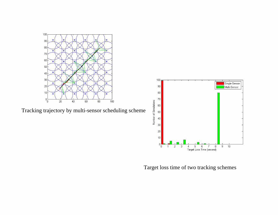
Tracking trajectory by multi-sensor scheduling scheme
Target loss time of two tracking schemes
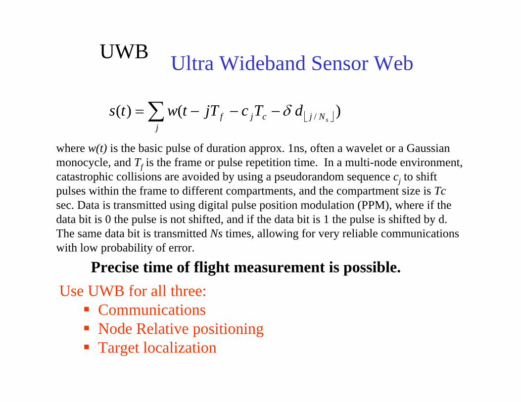
⎣ ⎦∑ −−−=j
Njcjf sdTcjTtwts )()( /δ
where w(t) is the basic pulse of duration approx. 1ns, often a wavelet or a Gaussian monocycle, and Tf is the frame or pulse repetition time. In a multi-node environment, catastrophic collisions are avoided by using a pseudorandom sequence cj to shift pulses within the frame to different compartments, and the compartment size is Tcsec. Data is transmitted using digital pulse position modulation (PPM), where if the data bit is 0 the pulse is not shifted, and if the data bit is 1 the pulse is shifted by d. The same data bit is transmitted Ns times, allowing for very reliable communications with low probability of error.
Ultra Wideband Sensor WebUWB
Precise time of flight measurement is possible.Use UWB for all three:
CommunicationsNode Relative positioningTarget localization
1 2
3
T
d d2
d3
x
y y
1 2
3
T
d d2
d3
x
x’y’
θ213
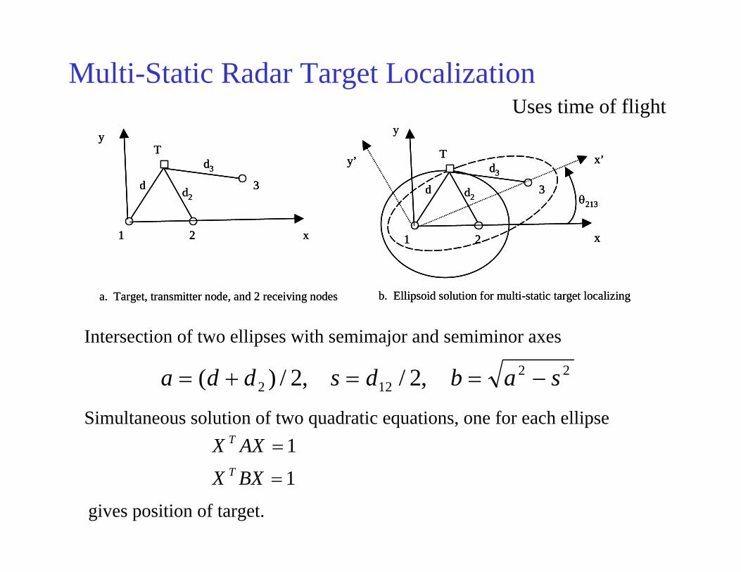
a. Target, transmitter node, and 2 receiving nodes b. Ellipsoid solution for multi-static target localizing
1 2
3
T
d d2
d3
x
y
1 2
3
T
d d2
d3
x
y y
1 2
3
T
d d2
d3
x
x’y’
θ213
1 2
3
T
d d2
d3
x
x’y’
θ213
a. Target, transmitter node, and 2 receiving nodes b. Ellipsoid solution for multi-static target localizing
Multi-Static Radar Target Localization
22122 ,2/,2/)( sabdsdda −==+=
Intersection of two ellipses with semimajor and semiminor axes
Simultaneous solution of two quadratic equations, one for each ellipse
11
=
=
BXXAXX
T
T
Uses time of flight
gives position of target.
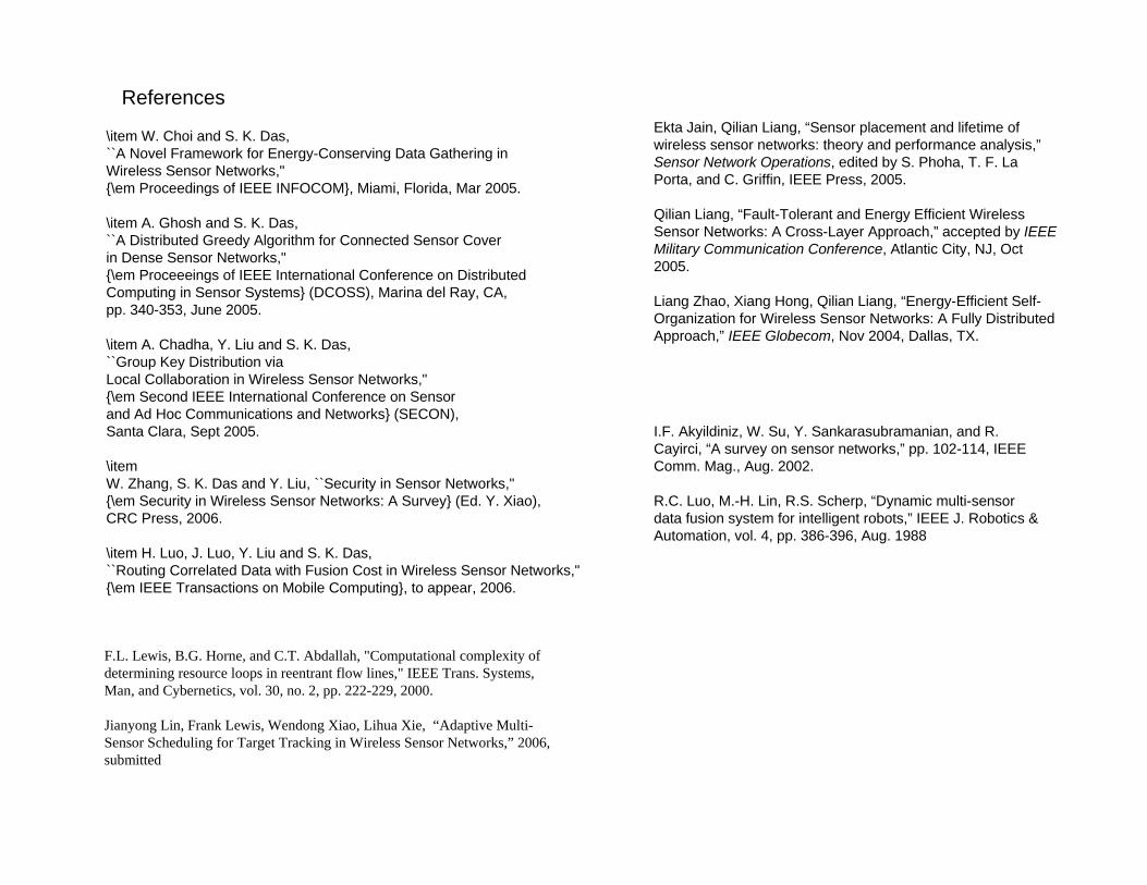
References
\item W. Choi and S. K. Das,``A Novel Framework for Energy-Conserving Data Gathering inWireless Sensor Networks,"{\em Proceedings of IEEE INFOCOM}, Miami, Florida, Mar 2005.
\item A. Ghosh and S. K. Das,``A Distributed Greedy Algorithm for Connected Sensor Coverin Dense Sensor Networks,"{\em Proceeeings of IEEE International Conference on DistributedComputing in Sensor Systems} (DCOSS), Marina del Ray, CA,pp. 340-353, June 2005.
\item A. Chadha, Y. Liu and S. K. Das,``Group Key Distribution viaLocal Collaboration in Wireless Sensor Networks,"{\em Second IEEE International Conference on Sensorand Ad Hoc Communications and Networks} (SECON),Santa Clara, Sept 2005.
\itemW. Zhang, S. K. Das and Y. Liu, ``Security in Sensor Networks,"{\em Security in Wireless Sensor Networks: A Survey} (Ed. Y. Xiao), CRC Press, 2006.
\item H. Luo, J. Luo, Y. Liu and S. K. Das,``Routing Correlated Data with Fusion Cost in Wireless Sensor Networks,"{\em IEEE Transactions on Mobile Computing}, to appear, 2006.
Ekta Jain, Qilian Liang, “Sensor placement and lifetime of wireless sensor networks: theory and performance analysis,”Sensor Network Operations, edited by S. Phoha, T. F. La Porta, and C. Griffin, IEEE Press, 2005.
Qilian Liang, “Fault-Tolerant and Energy Efficient Wireless Sensor Networks: A Cross-Layer Approach,” accepted by IEEE Military Communication Conference, Atlantic City, NJ, Oct 2005.
Liang Zhao, Xiang Hong, Qilian Liang, “Energy-Efficient Self-Organization for Wireless Sensor Networks: A Fully Distributed Approach,” IEEE Globecom, Nov 2004, Dallas, TX.
I.F. Akyildiniz, W. Su, Y. Sankarasubramanian, and R. Cayirci, “A survey on sensor networks,” pp. 102-114, IEEE Comm. Mag., Aug. 2002.
R.C. Luo, M.-H. Lin, R.S. Scherp, “Dynamic multi-sensor data fusion system for intelligent robots,” IEEE J. Robotics & Automation, vol. 4, pp. 386-396, Aug. 1988
F.L. Lewis, B.G. Horne, and C.T. Abdallah, "Computational complexity of determining resource loops in reentrant flow lines," IEEE Trans. Systems, Man, and Cybernetics, vol. 30, no. 2, pp. 222-229, 2000.
Jianyong Lin, Frank Lewis, Wendong Xiao, Lihua Xie, “Adaptive Multi-Sensor Scheduling for Target Tracking in Wireless Sensor Networks,” 2006, submitted

1.G. Vachtsevanos, F.L. Lewis, M. Roemer, A. Hess, B. Wu, Intelligent Fault Diagnosis and Prognosis for Engineering Systems, John Wiley, New York, 2006, to appear.
2.J. Mireles, F.L. Lewis, A. Gurel, and S. Bogdan, “Deadlock Avoidance Algorithms and Implementation, a Matrix-Based Approach,” in Deadlock Resolution in Computer-Integrated Systems, chapter 7, ed. Mengchu Zhou, Marcel Dekker, New York, 2004.
3.F.L. Lewis, “Wireless Sensor Networks,” in Smart Environments: Technologies, Protocols, Applications, ed. D.J. Cook and S.K. Das, Wiley, New York, 2004.
4.V. Giordano, F.L. Lewis, P. Ballal, and B. Turchiano, “Supervisory control for task assignment and resource dispatching in mobile wireless sensor networks,” in Cutting Edge Robotics, ed. V. Kordic, p. 133-152, 2005.
5.D.O. Popa and F.L. Lewis, “Algorithms for robotic deployment of WSN in adaptive sampling applications,” in Wireless Sensor Networks and Applications, ed. Y. Li, M. Thai, and W. Wu, Springer-Verlag, Berlin, 2005.
6.N. Swamy, O. Kuljaca, and F.L. Lewis, “Internet-based educational control systems lab using NetMeeting,” IEEE Trans. Education, vol. 45, no. 2, pp. 145-151, May 2002.
7.V. Giordano, P.Ballal, F.L. Lewis, B. Turchiano, J.B. Zhang, “Supervisory control of mobile sensor networks: Matrix formulation, simulation and implementation,” IEEE Trans. Systems, Man, Cybernetics, Part B, to appear, 2006.
8.B. Harris, D. Cook, and F.L. Lewis, "Automatically generating plans for manufacturing," J. Intelligent Systems, vol. 10, no. 3, pp. 279-319, 2000.
9.N. Swamy and F.L. Lewis, “Routing algorithms in a novel hierarchical mesh network,” Proc. IEEE 12th Symp. Mobile Computing, Bangalore, Nov. 2003.
10.A. Tiwari, F.L. Lewis, and S.S. Ge, “Wireless Sensor Networks for Machine Condition Based Monitoring,” Proc. Int. Conf. Control, Automation, Robotics, and Vision, pp. 461-467, invited paper, Kunming, China, Dec 2004.
11.V. Giordano, F.L. Lewis, J. Mireles, B. Turchiano, “Coordination control policy for mobile sensor networks with shared heterogeneous resources,” Proc. Int. Conf. Control & Automation, pp. 191-196, Budapest, June, 2005.
12.V. Giordano, F.L. Lewis, B. Turchaino, P. Ballal, V. Yeshala, “Matrix computational framework for discrete event control of wireless sensor networks with some mobile agents,” Proc. Mediterranean Conf. Control & Automation, Limassol, Cyprus, June 2005. This paper won an award at MED 05.
13.O. Kuljaca, N. Swamy, J. Gadewadikar, F.L. Lewis, “Transfer Function Illustration With Simple Electronic Circuits”, Proc. XXVII Int. Meeting MIPRO 2005, CE, Conference on Computers in Education, 2005.
14.D.O. Popa, K. Sreenath, and F.L. Lewis, “Robotic deployment for environmental sampling applications,” Proc. Int. Conf. Control and Applics., pp. 197-202, Budapest, June 2005.
Automation & Robotics Research Institute The University of Texas at Arlington
F.L. LewisMoncrief-O’Donnell Endowed Chair
Head, Controls & Sensors Group
Talk available online athttp://ARRI.uta.edu/acs
Wireless Sensor Networks