Embed Size (px)
Citation preview
Automating Feature Extraction with the ArcGIS SpatialAnalyst Extension
Author: Michael Hewett
Paper Abstract
LIDAR data can be overwhelming to use for manual feature extraction, and specialized
feature extraction software can be expensive to purchase. ArcGIS provides tools that can
be utilized to help get more out of LIDAR first, last and intensity returns through
automated processes. By following a few basic principles, it is possible to extract some
common features such as vegetation, stream banks, some buildings, etc. This session is
aimed at general ArcGIS users who wish to start making better use of their LIDAR
datasets by automating extraction of features with the ArcGIS Spatial Analyst extension.
Scope
Automated feature extraction is a challenge that continues to be heavily researched
throughout the GIS industry, and has still to be perfected. The purpose of this paper is to
provide understanding of some extraction techniques already available to LIDAR data
owners through the use of ArcGIS with the Spatial Analyst extension, and to stimulate
them to think more widely about their data. The approaches outlined in this paper in
most cases, will not provide the high quality feature outlines provided by some dedicated
feature extraction software or manual compilation, nor does this paper claim to provide
any new research into extraction techniques.
Untapped Wealth
Many organizations own or have access to LIDAR data. However, many of those
organizations only use their data in the form it was provided to them by the vendor and
for the one or two specific purposes for which it was acquired. LIDAR is a significant
investment by any organization, and it therefore makes sense to get the best use out of
that investment possible.
LIDAR data owners may not be tapping the potential of their data for a number of
reasons. The volumes of data can be overwhelming, especially for large areas. It can
appear difficult to extract meaningful data without specialist training and tools.
Specialist software can be expensive, especially if there is no specific project budgeted.
Data owners may not realize the potential of their data. For these reasons, and many
more, there are vast stores of current and historic LIDAR data that are being
underutilized.
However, if you have ArcGIS and the Spatial Analyst extension, you have the ability to
start getting more out of your data for yourself and your clients.

Why consider automated extraction.
Having stated that the results of approaches outlined in this paper are likely to be of a
lower quality those of dedicated feature extraction software or manual compilation, why
should you consider the approaches outlined below.
The answers are:
Cost:
The approaches below will only cost you a few man hours and some processor time to
explore if you have access to the Spatial Analyst extension. They will also allow you to
make low cost assessments of the value of larger investments in extraction technology or
projects.
Flexibility:
You can focus your methods to your goals, your data and your expertise. Once you start
to build your corporate knowledge in the processes you will quickly be able to add or
combine processes to meet new goals or needs, and you will be able modify the
parameters of the process to suit your production and data environment.
Speed:
Automated processes are generally faster than manual processes. At the very least, they
can reduce a series of manual interactions to one simple command. In some cases, you
can convert manual processes and assessments to fully automated processes.
Control:
You will be able develop processes specifically tailored to your data, and have the ability
to make changes to processing procedures as needed to meet the challenges of your
particular situation. You will also have the ability to take processes you have developed
and use them as modules of larger and more complex processes. Another aspect of
control is the ability to apply the same settings to processes repeatedly without the
possibility of typographic or other human error introducing inconsistencies between
datasets.
This paper will provide you with a starting point.
The quality issue
Before starting the exploration of your data, it is important to understand the level of
results you can expect. Some features will extract more cleanly than others. For
example, if you are extracting rural dams, you are likely to get fairly good results. If you
are trying to extract building outlines in a heavily treed suburban area, you results are
likely to be less clean. You should still be able to identify most buildings, but the
building outlines will usually not match the exact building shape. If you need that level
of quality in your results, then there are other options that better suit your needs. As a
general rule of thumb, the more homogenous you can make the feature you are trying to
extract, or the more you can make it stand out from the background data, the better your
results are likely to be.
The Basic Steps
Assess the available data.

LIDAR data comes in many forms. The data you hold will depend on the delivery
contract signed with the vendor. LIDAR usually has elevation and intensity components.
The elevation is the calculated elevation of the point from which the return was reflected.
Intensity it the brilliance of the return. Some surfaces absorb or scatter the laser more
than others, resulting in varying amounts of the laser being reflected back to the sensor.
LIDAR data also often contains First and Last return values. These are datasets with
returns from the first point the laser strikes and the last point the laser strikes. On solid
surfaces such as concrete, the first and last returns are often virtually the same. However,
in vegetated areas or with powelines, there is often a significant difference between the
first and last returns. This difference can be key information in identifying some features.
You may also have a Bare Earth dataset. This is a dataset filtered to remove as much
noise (vegetation, buildings, false returns, etc) as possible so as to display the data as if
the LIDAR was being taken of the ground surface only.
There are other forms of LIDAR available that are less common, and you may also have
other datasets you would wish to use to enhance your feature extraction such as imagery,
multi-spectral datasets, or radar, to name a few, but these will not be discussed in this
paper.
LIDAR First Z return of sample area (6ft Res)
LIDAR Last Z return of sample area (6ft Res)
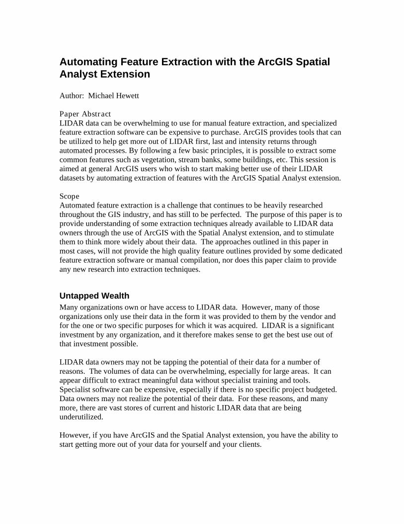
LIDAR Intensity Image of sample area (0.5ft Res)
Identify
Identify what makes the feature you want to extract different from the rest of the data in
your dataset. In some cases this will be easy, in others it will be harder. You don’t
necessarily have to think in terms of lines and points initially, but you will eventually

have to figure out a way to extract them from the data. For example, buildings are
usually higher than the surrounding area, lakes and dams are usually flat when they have
water in them. Powerlines are usually above the surrounding ground and form a
relatively straight line. Vegetation is usually not solid or at an even level.
Converting those observations to extraction terms is fairly simple, and the exraction
process for each will be outlined in more detail later in this paper.
Convert Data to a usable form.
In order to effectively process the data, you need to ensure it is in a form that you can
use. Spatial Analyst generally operates on rasters, so the best format for the LIDAR data
in this instance is raster format. ESRI provides a number of tools to convert XYZ tables
to points, and to convert points to raster, so you should be able to process your data into a
useable form fairly easily. It will depend on your data and your goals as to whether you
create floating point or integer rasters. Use a resolution that is appropriate to both your
LIDAR resolution and your extraction goal. You should try to pick a cell size that means
at least one LIDAR point will fall into each cell.
Enhance
Data enhancement will allow better extraction of specific features. It allows emphasis of
the characteristics that separate the sought after features from the surrounding data.
There are many options available to enhance the data. Layers may be combined, scaled
or converted in format. Mathematical calculations can be conducted, or other processes
such as a fill can be applied. Some examples are outlined in the examples below, but the
range of tools available in the Spatial Analyst toolbox will allow many other approaches.
Simplify the Data
After enhancing the data, it is useful to simplify the results. This will allow the results to
be more easily converted to lines or polygons. Thinning, grouping and conditional
extractions are just a few of the available options. The goal is to ensure each feature to
be extracted contains a common value within the field to be used as the extraction
criteria. During the extraction process, each unbroken grouping of identical values will
be converted to a feature.
Extract
Once the data is simplified it can be extracted to line or polygon features. The
Conversion toolbox contains tools to convert rasters to line, points or polygons. It is this
process that generates the final features.
Cleanup
While these processes allow the automated generation of features, it also may result in
the extraction of additional, undesired features. Automated and/or manual processes can
be applied to remove the additional unwanted features. For example, if buildings are
extracted from an elevation source, then there will be polygons representing the buildings
and the surrounding vegetation and land areas. By calculating the areas of the polygons
and removing, for example, those less than100sq feet or greater than 10000 sq feet, the
majority of the remaining polygons will be buildings. There still may be some additional

manual deletion required, but this should be simple and far quicker to achieve than the
manual compilation of the buildings.
Examples
Rapid Assessment:
Rapid assessments situations often require information that provides a general overview
of a situation without the specific detail that is generally expected in normal situations.
Example: You wish to assess the extent of damage to structures in the region after a
major storm. You had pre storm data and contracted a LIDAR Data provider to provide a
rapid response post storm dataset.
Extract buildings from both sets of data using the same process.
Building Extraction
Assess Data
Data Source: LIDAR First, last and intensity returns and Bare Earth.
Identify
In general, buildings are at least 6-8 feet above the immediately surrounding land. They
typically have vertical walls. Problems: They may be completely or partially under
overhanging vegetation. Surrounding land probably slopes, meaning buildings may start
and end at any elevation. There is little we can do about overhanging vegetation. It is
possible to identify the vegetation, but very difficult to identify which returns, if any, are
from the building under the vegetation.
Convert Data to Usable Form
If data is not in raster form, convert it to a raster. Cell size of one or two meters will
usually suffice. Additionally, integer rasters will be simpler and faster to process in this
case.
Enhance
Chose a standard value to be assumed as one story, then choose a number slightly less
than the one storey value. For this example, lets use 8 feet.
Use the Spatial Analyst/Math/Divide tool to divide the Last return elevation raster by 8,
ensuring the result is an integer. This will provide a raster that is approximate stories.
We used a value of slightly less than 1 storey to ensure that we didn’t lose any buildings
into the surrounding elevation data level.

Simplify
Use the Spatial Analyst/Math/Int tool to remove decimals from the divide result. You
should now have ‘regions’ of cells grouped by their ‘storey’ above sea level.
Extract
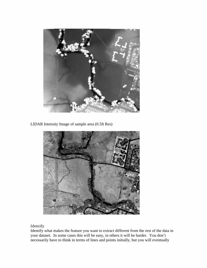
Use the Conversion Tools/From Raster/To Polygon tool to convert the results of the
Region Group process to polygons. You will now have polygons representing every
‘Storey group’ feature, land and buildings.
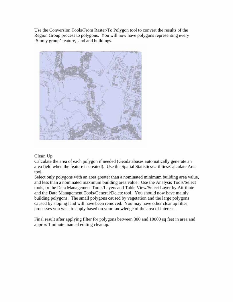
Clean Up
Calculate the area of each polygon if needed (Geodatabases automatically generate an
area field when the feature is created). Use the Spatial Statistics/Utilities/Calculate Area
tool.
Select only polygons with an area greater than a nominated minimum building area value,
and less than a nominated maximum building area value. Use the Analysis Tools/Select
tools, or the Data Management Tools/Layers and Table View/Select Layer by Attribute
and the Data Management Tools/General/Delete tool. You should now have mainly
building polygons. The small polygons caused by vegetation and the large polygons
caused by sloping land will have been removed. You may have other cleanup filter
processes you wish to apply based on your knowledge of the area of interest.
Final result after applying filter for polygons between 300 and 10000 sq feet in area and
approx 1 minute manual editing cleanup.
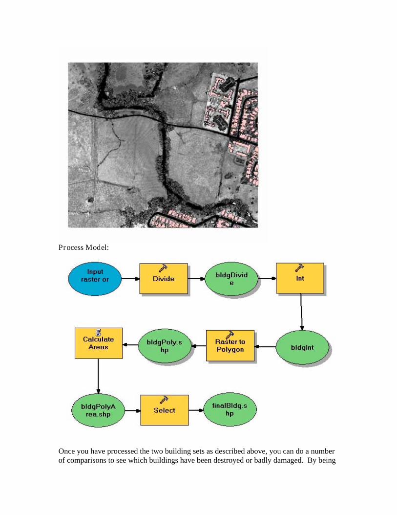
Process Model:
Once you have processed the two building sets as described above, you can do a number
of comparisons to see which buildings have been destroyed or badly damaged. By being

able to do the rough assessment in house through an automated process, you can expect
to have initial results faster than if you had to contract a company to do it for you or than
if you had to manually process the data. You could also use a combination of first and
last data from before the storm to identify likely vegetation overhang areas, and thus
enable special treatment of these areas if needed.
Change Assessment:
The example above could also be classified as change assessment. Alternatively, you
may wish to assess the density and area change to a vegetation tract over time by
comparing LIDAR clouds.
Example:
You wish to assess the change in coverage of trees over 30 feet tall in a forest region over
time.
Treed Area Extraction
Assess Data
Data Source: LIDAR First and Last for two or more epochs.
Identify
Trees are not a solid object. In most cases (extremely dense vegetation being the
exception) a first return will be off the top of the tree, while a last return will be off lower
parts of the tree or the ground. Therefore, by identifying areas where the first and last
returns are 30 feet or more apart it is possible to identify where trees over 30 feet are
growing. There are two approaches to this problem. If you have paired first and last
datasets (ie you can identify and pair the first and last returns of individual pulses) then
you can use the difference of the first and last pulse returns as your base data. This is
probably the preferred approach, but you must remember to allow for any slope in the ray
path when calculating the height. The second approach is to use the first and last points
to create unpaired elevation datasets. This means that unrelated pulses may interact to
generate a height difference for a particular cell. Unless data holders have structured
their LIDAR storage in such a manner as to maintain pulse correlations, then this is the
option that will have to be used, so will be the option outlined here.
Covert Data to usable form.
Convert the first and last returns for each epoch to raster format. Carefully consider your
cell size based on vegetation variation, ground elevation changes and the detail resolution
required by your results. If applicable, also consider the best method for converting
points to raster (min, max, mean, etc).
Enhance
For each epoch, divide the first return by the height of the trees you wish to examine.

Next, convert the results of the last step to integers:
In order to identify which polygons are tree polygons that meet your criteria, you now
need to find the areas where there are 30 foot differences between first and last returns.

Subtract the last returns from the first returns.
Next, convert the values to absolutes using Spatial Analyst/Math/Abs.

This is necessary because this process deals with grouped cell values containing multiple
disassociated ray values rather than first and last on a ray.
Simplify
Use Spatial Analyst/Conditional/Con to extract cells where the calculated elevation
difference is greater than 30 feet.
Extract
Convert the integer results of the first return divide into polygons.
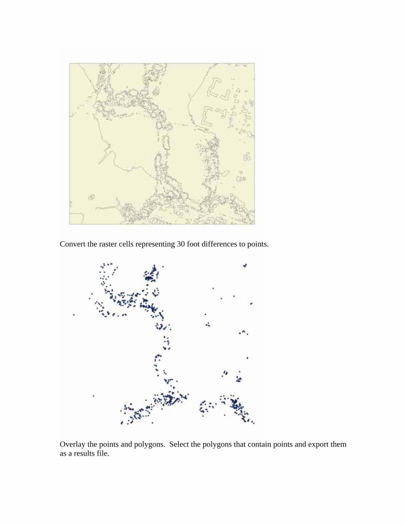
Convert the raster cells representing 30 foot differences to points.
Overlay the points and polygons. Select the polygons that contain points and export them
as a results file.
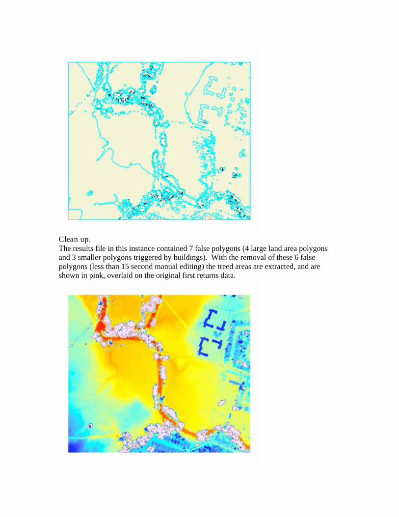
Clean up.
The results file in this instance contained 7 false polygons (4 large land area polygons
and 3 smaller polygons triggered by buildings). With the removal of these 6 false
polygons (less than 15 second manual editing) the treed areas are extracted, and are
shown in pink, overlaid on the original first returns data.
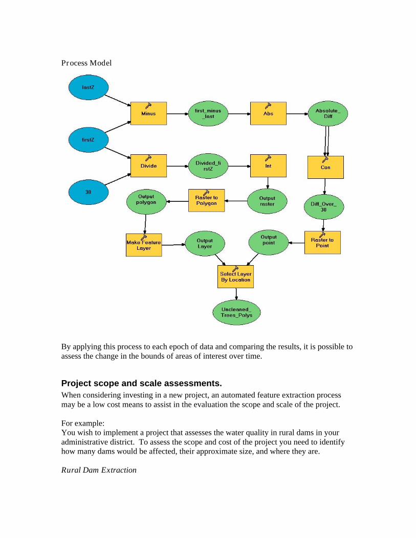
Process Model
By applying this process to each epoch of data and comparing the results, it is possible to
assess the change in the bounds of areas of interest over time.
Project scope and scale assessments.
When considering investing in a new project, an automated feature extraction process
may be a low cost means to assist in the evaluation the scope and scale of the project.
For example:
You wish to implement a project that assesses the water quality in rural dams in your
administrative district. To assess the scope and cost of the project you need to identify
how many dams would be affected, their approximate size, and where they are.
Rural Dam Extraction

Assess Data
Data Source: LIDAR First, last and intensity returns and Bare Earth.
Identify
A rural dam, when full, will have no slope due to a flat water surface, while the
surrounding land will have some slope component. Dams should have a raised dam wall.
Possible problems: Dams are not always full, LIDAR in water can have uneven Z
readings due to different turbidity and surface wave properties, there may be other flat
areas such as flat rooftops or road sections, dry dams may not be visible on the intensity
image.
Convert Data to Usable Form
If data is not in raster form, convert it to a raster. Cell size of several feet will usually
suffice.
The image below is an elevation raster of a section of rural land at 1m pixel resolution.
Enhance
Use the Spatial Analyst/Hydrology/Fill tool to fill in dips in the ground. By choosing the
settings that will fill until the overflow level, all dams and other depressions will have
their Z value raised to the lowest overflow level of the dam/hollow. Raised roads,
bridges etc will cause some false positives, as will small natural depressions. These will
be fixed in the clean up process.

Convert the filled elevation raster to a slope raster using the Spatial
Analyst/Surface/Slope tool.
Simplify

Use the Spatial Analyst/Conditional/Con tool to extract all areas where slope < 0.01.
Extract
Use the Conversion Tools/From Raster/To Polygon tool to convert the results of the
simplify process to polygons. You will now have polygons representing all zero slope
areas. These will contain the false positives mentioned in the Enhance step.

Clean Up
To remove false positives:
Calculate the area of each polygon if needed (Geodatabases automatically generate an
area field when the feature is created). Use the Spatial Statistics/Utilities/Calculate Area
tool.
Select only polygons with an area of greater than a nominated minimum dam area value.
(eg 500sq feet). Use the Analysis Tools/Select tools, or the Data Management
Tools/Layers and Table View/Select Layer by Attribute and the Data Management
Tools/General/Delete tool.
If you have road centerlines for the area you can use a buffered road centerline to select
and delete the false positives caused by raised roads. If not, you may want to remove
these problem areas manually using the intensity image as a guide, or you may wish to
attempt an extraction of the roads for intensity or other data, then use those results to
clean up the problem areas. Ultimately, you will have a reasonably good assessment of
the dams in the area in question.
Process Model

A starting point for more detailed work.
You may find it faster/easier/cheaper in some instances to generate a coarse dataset
automatically then spend your manpower on refining that dataset than to build the dataset
through entirely manual processes.
In all of the above examples it is possible to identify less than ideal elements of the
results. Polygons do not exactly match the features they represent. Smaller or borderline
features may have been missed, and so on. With this in mind, you may want to improve
on the results through further manual processing or refining the automated processing. In
most cases, this additional processing will take less resources than creating the data from
scratch through non automated means.
Economies of scale
While it may not seem worthwhile to develop automated processes for the area shown in
the demonstration screenshots, the development time for a 1sq mile area or a 250sq mile
area are the same. The only differences in production are processor time and cleanup
time. With the longest manual cleanup time for the demonstration processes being less
than 1 minute, the reduction in effort for large projects quickly outstrip the effort in
manually producing even a coarse dataset. Automated processes also have the advantage
of being able to run at night when workstations are typically less busy, thereby increasing
the productivity of hardware resources held by an organization.

Conclusion
The processes outlined in this paper are limited in scope due to the need for a realistically
brief paper. There are many other possibilities and uses for even the limited set of data
used for demonstration. By applying the basic principles outlined in this paper, it is
possible to add value to almost any LIDAR dataset. Although the results from theses
processes are generally coarse, there are many instances where the higher quality results
available through manual compilation and dedicated extraction software are not needed,
and the considerable extra expense makes them uneconomical for many uses. This is
particularly true where the need is an estimation, approximation or rough guide.
Consider the needs of your organization, clients or potential clients and start to unlock the
untapped wealth of your LIDAR datasets.
Data Acknowledgements:
Permissions to the raw LIDAR data used for examples in this paper were kindly granted
by the data owners:
USDA-NRCS, Wyoming for source data used in the rural dams example.
Medina Consultants Inc for all other source data.
References:
ESRI ArcGIS software documentation, Version 9.0.
Author Information
Michael Hewett
GIS Analyst
Sanborn Map Company, Inc
1935 Jamboree Drive
Suite 100
Colorado Springs, CO 80920
Phone: 719.593.0093
email: [email protected]