Automatic Wave Equation Migration Velocity Analysis

Peng Shen, William. W. Symes

HGRG, Total E&PCAAM, Rice University

This work supervised by Dr. Henri Calandra at Total E&PThank to Dr. Scott Morton at Amerada Hess Corp.

Velocity Analysis

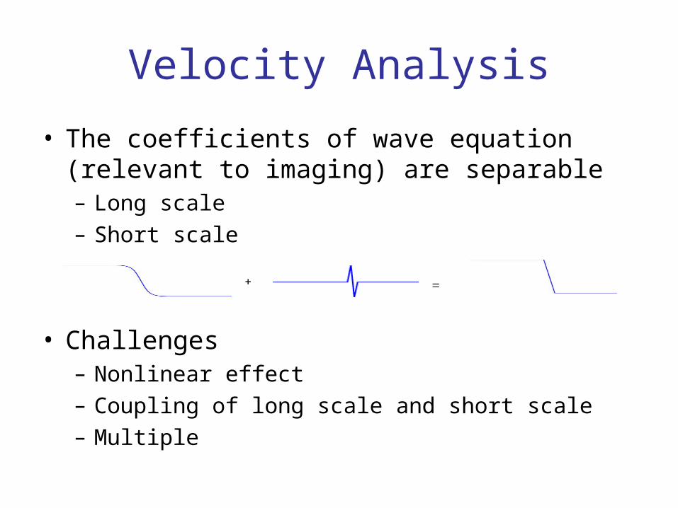
• The coefficients of wave equation (relevant to imaging) are separable– Long scale– Short scale

• Challenges– Nonlinear effect– Coupling of long scale and short scale– Multiple

Methods of Velocity Analysis

• Data domain objectives– Waveform inversion– Stereotomography

• Image domain objectives– WE-Migration forward, ray tracing inverse– WE-Migration forward, WE-Migration inverse

Outline

• Theory– Objective function– Gradient

• Calculation• Physical meaning• Smoothing

– Aliasing

• Examples– Angle ~ Offset– Reconstruct short scale and large scale variations

Generalized Born Modeling

Reflection occurs instantaneously with no separation in space.

Reflection occurs instantaneously separated by a finite distance.

Do not require to use the true velocity.

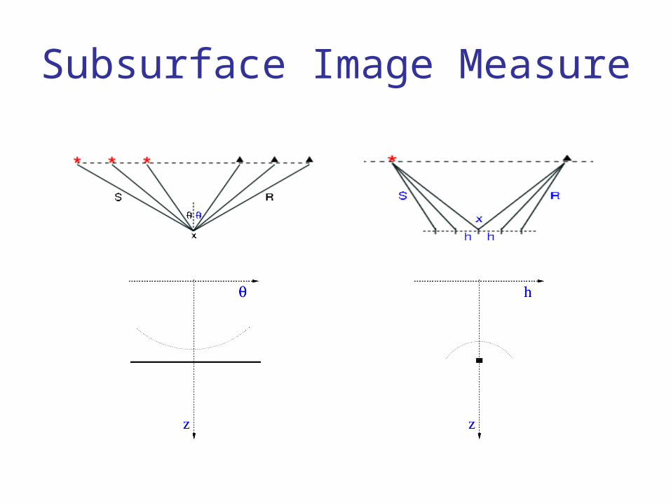
Subsurface Image Measure

Example

Data generated with caustic, migrated using correct and background velocity.

Differential Semblance

)()(),( hxfhxIh ||),(|| hxhIh

)(),( xgxI ),(),(

hxIRxI

hh

Offset domain:

Angle domain:

Pseudo-differential operator of00,1S

The objective function is smooth in velocity and is suitable for automatic velocity updating (Stolk & Symes, 2003).

Gradient Calculation

}{ 2*

hh

c Ihc

IrealJ

}{2

2*

*

hh

c RIRc

IrealJ

Offset:

Angle:

Gradient: Physical Meaning

Single scattering, constructive interference occurs at zero offset.

Gradient: Physical Meaning

“Two scatterings”, constructive interference occurs on ray segments.

Smoothing

• Problem– The raw gradient is singular with full data bandwidth.

• Solution– Confine the velocity model to the space of B-splines.

• Controlled degree of smoothness• Compactly supported basis

• Implication– Projection to B-spline model space.– B : forward interpolation - sparse dense– B*: adjoint projection - sparse dense

Example

Flat reflector, constant velocity Projected gradient using BB* for one shot

The gradient + B-spline projection reconstructs wide ray paths which are controlled by the degree of smoothness supplied.

Optimization on B-spline space

Aliasing

• We care not only the image in zero offset but also its move-out in non-zero offsets.

• There are many non-zero offset aliasing effects.– Data pre-conditioning.– Acquisition edge effect.

Kinematics

u

zhH

c

ZH 2222 )(

0);,(

)()()( 22222

HhzF

ZHc

uzHh

Kinematics of Image in Offset

u<c u=c u>c

c

u

Z

z

Z

h

1

)1( 22

2

22

2

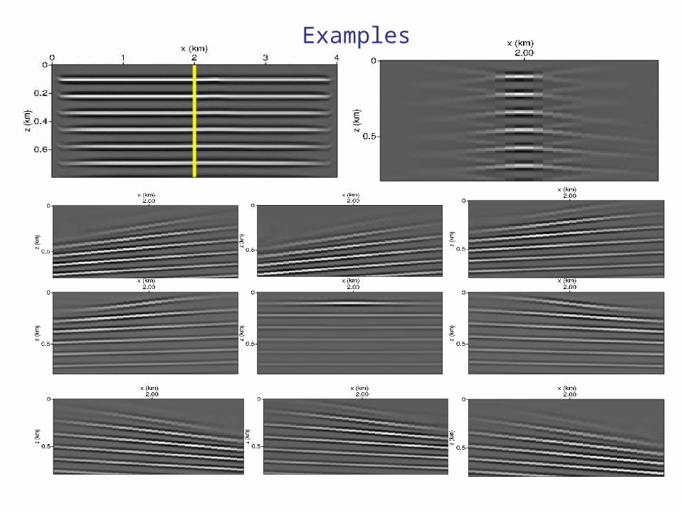
Examples

Anti-aliasing

Aliasing reduced but loose some image Strong aliasing

Examples

• Born data

• Full data with rough model

• Initial model construction

• Optimization starting with v(z)

Born Data Examples

Smooth Marmousi velocity model, singular reflectivity, one-way wave simulation, acquisition full spread, receiver dense on surface.

Starting Model

Starting model, large horizontal scales, assumed to be obtainable through conventional velocity analysis tools.

Optimization: 150m x 200m B-spline grid.

Initial Image

Optimized Image

Optimized image using angle domain DSO.

Optimized image using offset domain DSO.

Optimized Velocity

Optimized using angle domain DSO.

Optimized using offset domain DSO.

Initial Angle and Offset Gathers

Top: offset gathers, bottom: angle gathers

Optimized Gathers (angle driven)

Top: offset gathers (not used in the optimization), bottom: angle gathers.

Optimized Gathers (offset driven)

Top: offset gathers, bottom: angle gathers (not used in the optimization)

Velocity Difference

Difference between optimized velocity and the projected true velocity (optimized by angle DSO).

Difference between optimized velocity and the projected true velocity (optimized by offset DSO).

Rough Marmousi Model

Data generated using full wave equation simulation, acquisition split spread, receiver spacing 25m, receiver array across entire surface.

Optimization: offset driven, B-spline grid 120m by 22m.

Initial Velocity and Image

Initial velocity model, corresponds to B-spline grid 900m by 300m.

Initial image

Optimized Velocity and Image

Optimized velocity at 99th iteration Optimized image at 99th iteration

Optimized Velocity and Image

Optimized velocity at 49th iteration Optimized image at 49th iteration

The optimization is stable and convergent.

Obtain a Starting Model

A v(z) starting model.

Optimization: run up to 10Hz, coarse B-spline grid 800m by 400m, 500m by 200m.

Optimized Velocity

800m by 400m, DSO optimized. Projected from the true model.

500m by 200m, DSO optimized. Projected from the true model.

Null Space

Optimized image at 20th iteration. Optimized image at 49th iteration.

Starting with v(z) Velocity

Start from v(z) velocity model, increase frequency and spatial resolution in two steps.

Conclusions

• The angle domain DSO is not superior to offset domain DSO.

• The velocity analysis within migration is a promising direction to pursue.

• The adjoint-differential-migration provides an ideal platform for AWEMVA.