Instructor: Preethi Jyothi Mar 23, 2017

Automatic Speech Recognition (CS753)Lecture 18: Search & Decoding (Part I)Automatic Speech Recognition (CS753)

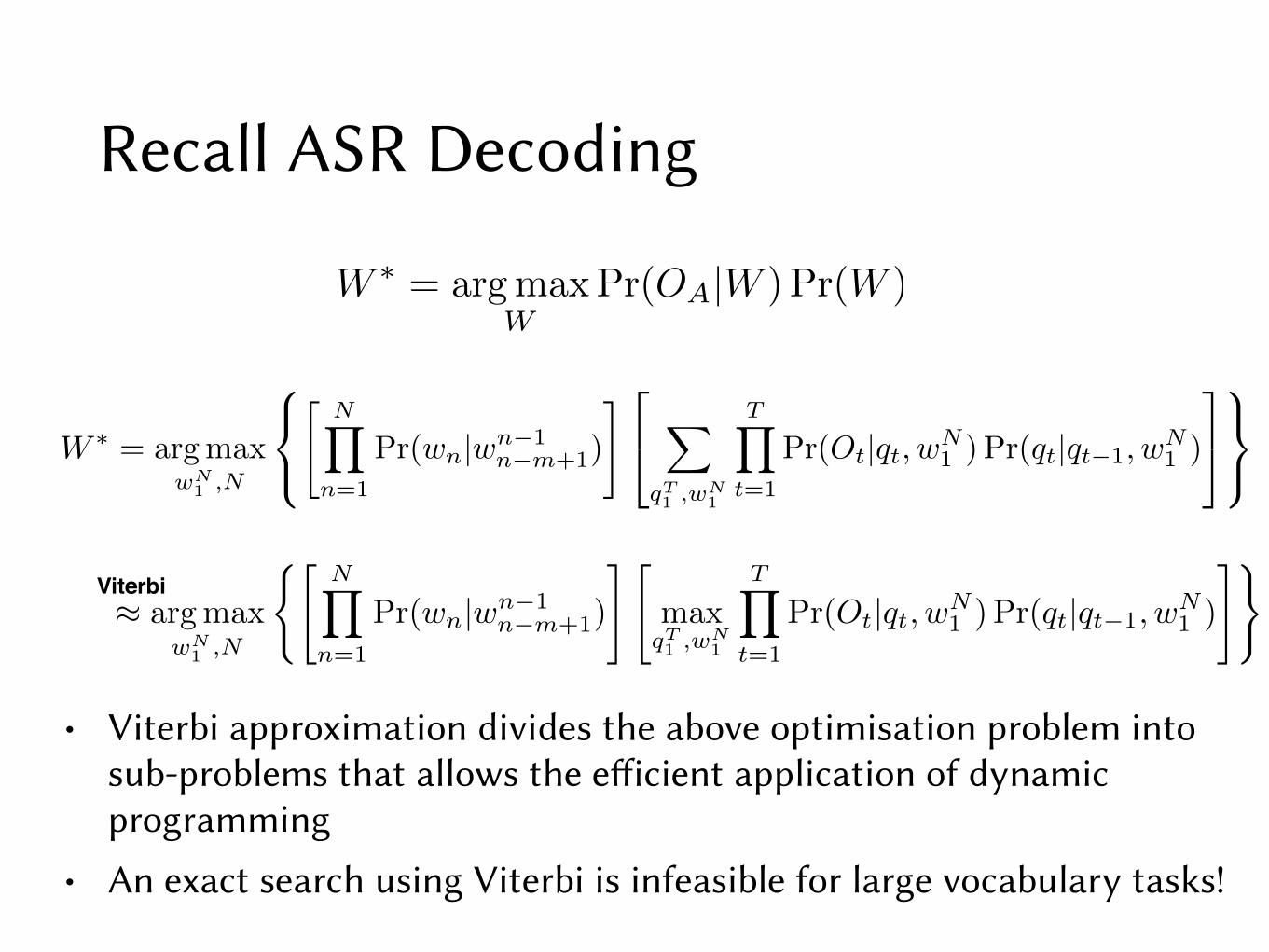
Recall ASR Decoding

W ⇤= argmax

WPr(OA|W ) Pr(W )

W ⇤= argmax

wN1 ,N

8<

:

"NY

n=1

Pr(wn|wn�1n�m+1)

#2

4X

qT1 ,wN1

TY

t=1

Pr(Ot|qt, wN1 ) Pr(qt|qt�1, w

N1 )

3

5

9=

;

⇡ argmax

wN1 ,N

("NY

n=1

Pr(wn|wn�1n�m+1)

#"max

qT1 ,wN1

TY

t=1

Pr(Ot|qt, wN1 ) Pr(qt|qt�1, w

N1 )

#)Viterbi

• Viterbi approximation divides the above optimisation problem into sub-problems that allows the efficient application of dynamic programming

• An exact search using Viterbi is infeasible for large vocabulary tasks!

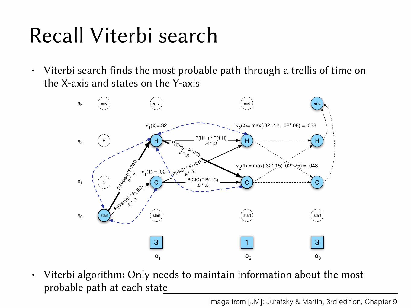
Recall Viterbi search• Viterbi search finds the most probable path through a trellis of time on

the X-axis and states on the Y-axis

• Viterbi algorithm: Only needs to maintain information about the most probable path at each state

9.5 • HMM TRAINING: THE FORWARD-BACKWARD ALGORITHM 13

start

H

C

H

C

H

C

end

P(C|start)

* P(3|C)

.2 * .1

P(H|H) * P(1|H).6 * .2

P(C|C) * P(1|C).5 * .5

P(C|H) * P(1|C).3 * .5

P(H|C) * P(1|H)

.4 * .2

P(H|

start)

*P(3

|H)

.8 *

.4v1(2)=.32

v1(1) = .02

v2(2)= max(.32*.12, .02*.08) = .038

v2(1) = max(.32*.15, .02*.25) = .048

start start start

t

C

H

end end endqF

q2

q1

q0

o1 o2 o3

3 1 3

Figure 9.12 The Viterbi backtrace. As we extend each path to a new state account for the next observation,we keep a backpointer (shown with broken lines) to the best path that led us to this state.

Finally, we can give a formal definition of the Viterbi recursion as follows:

1. Initialization:

v1( j) = a0 jb j(o1) 1 j N (9.20)

bt1( j) = 0 (9.21)

2. Recursion (recall that states 0 and qF are non-emitting):

vt( j) =N

maxi=1

vt�1(i)ai j b j(ot); 1 j N,1 < t T (9.22)

btt( j) =N

argmaxi=1

vt�1(i)ai j b j(ot); 1 j N,1 < t T (9.23)

3. Termination:

The best score: P⇤= vT (qF) =N

maxi=1

vT (i)⇤aiF (9.24)

The start of backtrace: qT⇤= btT (qF) =N

argmaxi=1

vT (i)⇤aiF (9.25)

9.5 HMM Training: The Forward-Backward Algorithm

We turn to the third problem for HMMs: learning the parameters of an HMM, thatis, the A and B matrices. Formally,

Image from [JM]: Jurafsky & Martin, 3rd edition, Chapter 9

ASR Search Network

0the birds

are

boy is

walking

d ax

b

oy

b

Network of words

Network of phones

Network of HMM states

Time-state trellisw

ord 1

wor

d 2w

ord 3

Time, t →

Viterbi search over the large trellis

• Exact search is infeasible for large vocabulary tasks

• Unknown word boundaries

• Ngram language models greatly increase the search space

• Solutions

• Compactly represent the search space using WFST-based optimisations

• Beam search: Prune away parts of the search space that aren’t promising

Viterbi search over the large trellis

• Exact search is infeasible for large vocabulary tasks

• Unknown word boundaries

• Ngram language models greatly increase the search space

• Solutions

• Compactly represent the search space using WFST-based optimisations

• Beam search: Prune away parts of the search space that aren’t promising

Two main WFST Optimizations

Recall not all weighted transducers are determinizable

To ensure determinizability of L ○ G, introduce disambiguation symbols in L to deal with homophones in the lexicon

read : r eh d #0 red : r eh d #1

• Use determinization to reduce/eliminate redundancy

Propagate the disambiguation symbols as self-loops back to C and H. Resulting machines are H̃, C̃, L̃

• Use determinization to reduce/eliminate redundancy

• Use minimization to reduce space requirements

Two main WFST Optimizations

Minimization ensures that the final composed machine has minimum number of states

Final optimization cascade:

N = πε(min(det(H̃ ○ det(C̃ ○ det(L̃ ○ G)))))

Replaces disambiguation symbols in input alphabet of H̃ with ε

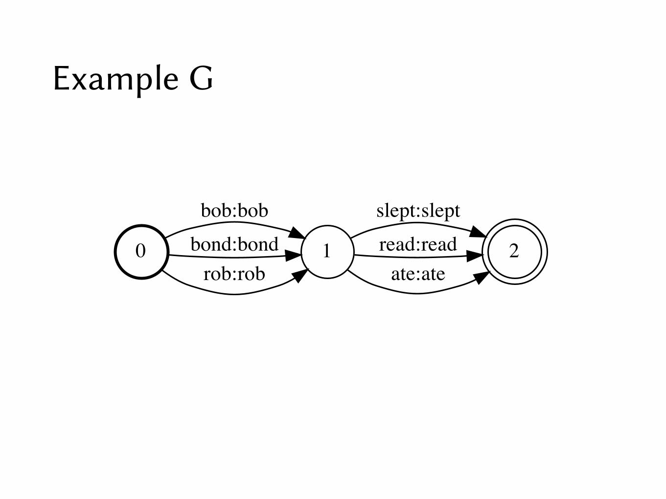
Example G

0 1

bob:bobbond:bondrob:rob

2

slept:sleptread:readate:ate

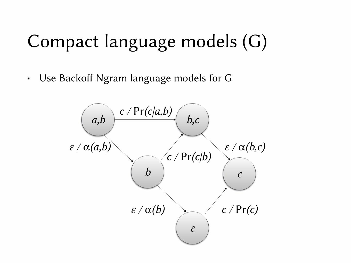
Compact language models (G)

• Use Backoff Ngram language models for G

a,b b,c

b

ε

c

c / Pr(c|a,b)

ε / α(a,b)c / Pr(c|b)

ε / α(b,c)

ε / α(b) c / Pr(c)

Example G

0 1

bob:bobbond:bondrob:rob

2

slept:sleptread:readate:ate

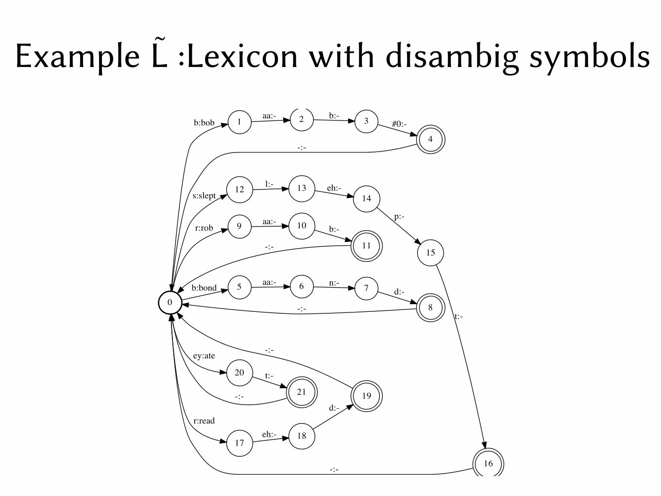
Example L̃ :Lexicon with disambig symbols

0

1b:bob

5b:bond

9r:rob

12s:slept

17

r:read

20

ey:ate

2aa:-

6aa:-

10aa:-

13l:-

18eh:-

21

t:-

3b:-

4

#0:-

-:-

7n:-

8

d:-

-:-

11

b:-

-:-

14eh:-

15

p:-

16

t:-

-:-

19d:-

-:-

-:-

L̃ ○ G

0

1b:bob

2b:bond

3

r:rob

4aa:-

5aa:-

6aa:-

7b:-

8n:-

9b:-

10#0:-

11d:- 12

-:-

-:-

-:-

13s:slept

14r:read

15

ey:ate

16l:-

17eh:-

18t:-

19eh:-

20d:-

21p:- 22t:-

det(L̃ ○ G)

0

1b:-

2r:rob

3aa:-

4aa:-

5b:bob

6n:bond

7b:-

8#0:-

9d:- 10

-:-

-:-

-:-

11r:read

12s:slept

13

ey:ate

14eh:-

15l:-

16t:-

17d:-

18eh:- 19p:- 20t:-

min(det(L̃ ○ G))

0

1b:-

2r:rob

3aa:-

4aa:-

5b:bob

6n:bond 7

b:-

#0:-

d:- 8-:-

9r:read

10s:slept 11

ey:ate

12eh:-

13l:-14t:-

d:-

15eh:- p:-

det(L̃ ○ G)

0

1b:-

2r:rob

3aa:-

4aa:-

5b:bob

6n:bond

7b:-

8#0:-

9d:- 10

-:-

-:-

-:-

11r:read

12s:slept

13

ey:ate

14eh:-

15l:-

16t:-

17d:-

18eh:- 19p:- 20t:-

Viterbi search over the large trellis

• Exact search is infeasible for large vocabulary tasks

• Unknown word boundaries

• Ngram language models greatly increase the search space

• Solutions

• Compactly represent the search space using WFST-based optimisations

• Beam search: Prune away parts of the search space that aren’t promising

Beam pruning• At each time-step t, only retain those nodes in the time-state

trellis that are within a fixed threshold δ (beam width) of the best path

• Given active nodes from the last time-step:

• Examine nodes in the current time-step …

• … that are reachable from active nodes in the previous time-step

• Get active nodes for the current time-step by only retaining nodes with hypotheses that score close to the score of the best hypothesis

Beam search

• Beam search at each node keeps only hypotheses with scores that fall within a threshold of the current best hypothesis

• Hypotheses with Q(t, s) < δ ⋅ max Q(t, s’) are pruned

here, δ controls the beam width

• Search errors could occur if the most probable hypothesis gets pruned

• Trade-off between balancing search errors and speeding up decoding

Static and dynamic networks

• What we’ve seen so far: Static decoding graph

• H ○ C ○ L ○ G

• Determinize/minimize to make this graph more compact

• Another approach: Dynamic graph expansion

• Dynamically build the graph with active states on the fly

• Do on-the-fly composition with the language model G

• (H ○ C ○ L) ○ G

Multi-pass search

• Some models are too expensive to implement in first-pass decoding (e.g. RNN-based LMs)

• First-pass decoding: Use simpler model (e.g. Ngram LMs)

• to find most probable word sequences

• and represent as a word lattice or an N-best list

• Rescore first-pass hypotheses using complex model to find the best word sequence

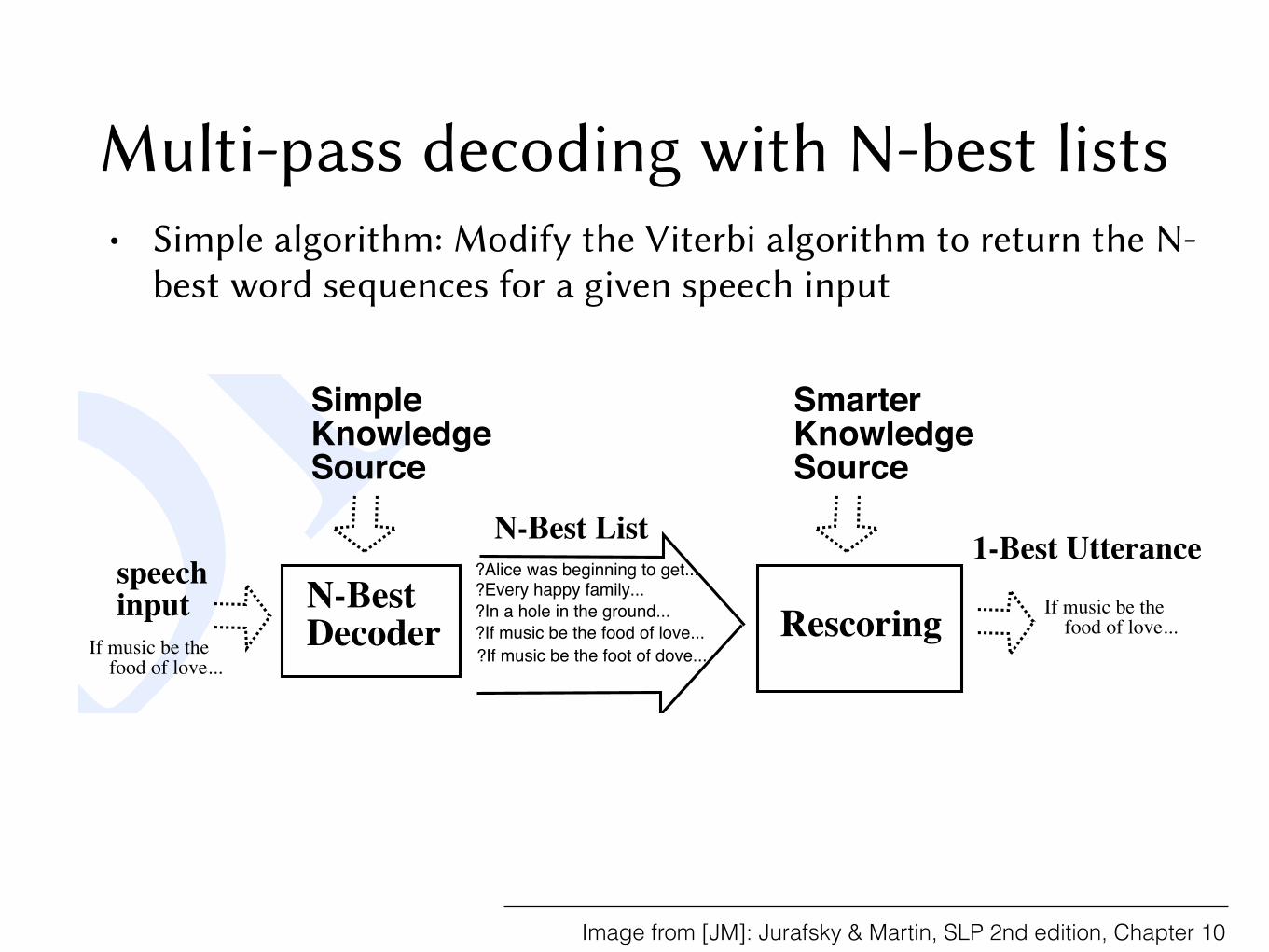
Multi-pass decoding with N-best lists

DRAFTSection 10.1. Multipass Decoding: N-best lists and lattices 3

to wy didn’t include wz (i.e., P(wy|wq,wz) was low for all q). Advanced probabilisticLMs like SCFGs also violate the same dynamic programming assumptions.

There are two solutions to these problems with Viterbi decoding. The most com-mon is to modify the Viterbi decoder to return multiple potential utterances, insteadof just the single best, and then use other high-level language model or pronunciation-modeling algorithms to re-rank these multiple outputs (Schwartz and Austin, 1991;Soong and Huang, 1990; Murveit et al., 1993).

The second solution is to employ a completely different decoding algorithm, suchas the stack decoder, or A∗ decoder (Jelinek, 1969; Jelinek et al., 1975). We beginSTACK DECODER

A∗ in this section with multiple-pass decoding, and return to stack decoding in the next

section.In multiple-pass decoding we break up the decoding process into two stages. In

the first stage we use fast, efficient knowledge sources or algorithms to perform a non-optimal search. So for example we might use an unsophisticated but time-and-spaceefficient language model like a bigram, or use simplified acoustic models. In the seconddecoding pass we can apply more sophisticated but slower decoding algorithms on areduced search space. The interface between these passes is an N-best list or wordlattice.

The simplest algorithm for multipass decoding is to modify the Viterbi algorithmto return the N-best sentences (word sequences) for a given speech input. SupposeN-BEST

for example a bigram grammar is used with such an N-best-Viterbi algorithm to returnthe 1000 most highly-probable sentences, each with their AM likelihood and LM priorscore. This 1000-best list can now be passed to a more sophisticated language modellike a trigram grammar. This new LM is used to replace the bigram LM score ofeach hypothesized sentence with a new trigram LM probability. These priors can becombined with the acoustic likelihood of each sentence to generate a new posteriorprobability for each sentence. Sentences are thus rescored and re-ranked using thisRESCORED

more sophisticated probability. Fig. 10.1 shows an intuition for this algorithm.

If music be the food of love...

If music be the food of love...

N-Best List

?Every happy family...?In a hole in the ground...?If music be the food of love...?If music be the foot of dove...

?Alice was beginning to get...

N-BestDecoder

SmarterKnowledgeSource

1-Best Utterance

Simple KnowledgeSource

speechinput Rescoring

Figure 10.1 The use of N-best decoding as part of a two-stage decoding model. Effi-cient but unsophisticated knowledge sources are used to return the N-best utterances. Thissignificantly reduces the search space for the second pass models, which are thus free tobe very sophisticated but slow.

There are a number of algorithms for augmenting the Viterbi algorithm to generateN-best hypotheses. It turns out that there is no polynomial-time admissible algorithm

• Simple algorithm: Modify the Viterbi algorithm to return the N-best word sequences for a given speech input

Image from [JM]: Jurafsky & Martin, SLP 2nd edition, Chapter 10

Multi-pass decoding with N-best lists• Simple algorithm: Modify the Viterbi algorithm to return the N-

best word sequences for a given speech input

Image from [JM]: Jurafsky & Martin, SLP 2nd edition, Chapter 10

• N-best lists aren’t as diverse as we’d like. And, not enough information in N-best lists to effectively use other knowledge sources

DRAFT

4 Chapter 10. Speech Recognition: Advanced Topics

for finding the N most likely hypotheses (?). There are however, a number of ap-proximate (non-admissible) algorithms; we will introduce just one of them, the “ExactN-best” algorithm of Schwartz and Chow (1990). In Exact N-best, instead of each statemaintaining a single path/backtrace, we maintain up to N different paths for each state.But we’d like to insure that these paths correspond to different word paths; we don’twant to waste our N paths on different state sequences that map to the same words. Todo this, we keep for each path the word history, the entire sequence of words up tothe current word/state. If two paths with the same word history come to a state at thesame time, we merge the paths and sum the path probabilities. To keep the N best wordsequences, the resulting algorithm requires O(N) times the normal Viterbi time.

AM LMRank Path logprob logprob1. it’s an area that’s naturally sort of mysterious -7193.53 -20.252. that’s an area that’s naturally sort of mysterious -7192.28 -21.113. it’s an area that’s not really sort of mysterious -7221.68 -18.914. that scenario that’s naturally sort of mysterious -7189.19 -22.085. there’s an area that’s naturally sort of mysterious -7198.35 -21.346. that’s an area that’s not really sort of mysterious -7220.44 -19.777. the scenario that’s naturally sort of mysterious -7205.42 -21.508. so it’s an area that’s naturally sort of mysterious -7195.92 -21.719. that scenario that’s not really sort of mysterious -7217.34 -20.7010. there’s an area that’s not really sort of mysterious -7226.51 -20.01

Figure 10.2 An example 10-Best list from the Broadcast News corpus, produced by theCU-HTK BN system (thanks to Phil Woodland). Logprobs use log10; the language modelscale factor (LMSF) is 15.

The result of any of these algorithms is anN-best list like the one shown in Fig. 10.2.In Fig. 10.2 the correct hypothesis happens to be the first one, but of course the reasonto use N-best lists is that isn’t always the case. Each sentence in an N-best list is alsoannotated with an acoustic model probability and a language model probability. Thisallows a second-stage knowledge source to replace one of those two probabilities withan improved estimate.

One problem with an N-best list is that when N is large, listing all the sentencesis extremely inefficient. Another problem is that N-best lists don’t give quite as muchinformation as we might want for a second-pass decoder. For example, we might wantdistinct acoustic model information for each word hypothesis so that we can reapply anew acoustic model for the word. Or we might want to have available different startand end times of each word so that we can apply a new duration model.

For this reason, the output of a first-pass decoder is usually a more sophisticatedrepresentation called a word lattice (Murveit et al., 1993; Aubert and Ney, 1995). AWORD LATTICE

word lattice is a directed graph that efficiently represents much more information aboutpossible word sequences.1 In some systems, nodes in the graph are words and arcs are

1 Actually an ASR lattice is not the kind of lattice that may be familiar to you from mathematics, since it isnot required to have the properties of a true lattice (i.e., be a partially ordered set with particular properties,such as a unique join for each pair of elements). Really it’s just a graph, but it is conventional to call it a

Multi-pass decoding with lattices• ASR lattice: Weighted automata/directed graph representing

alternate word hypotheses from an ASR system

so, it’sit’s

there’s

that’s

that scenario

an area that’s naturally sort of mysterious

the not really

Multi-pass decoding with lattices• Confusion networks/sausages: Lattices that show competing/

confusable words and can be used to compute posterior probabilities at the word level

it’sthere’sthat’s

that scenario

an area that’s naturally sort of mysterious

the

not