Embed Size (px)
Citation preview
Correspondence to: [email protected]
http://dx.doi.org/10.5565/rev/elcvia.680
Recommended for acceptance by Jorge Bernal
ELCVIA ISSN: 1577-5097
Published by Computer Vision Center / Universitat Autonoma de Barcelona, Barcelona, Spain
Electronic Letters on Computer Vision and Image Analysis 14(1):1-20, 2015
Automatic Segmentation of Optic Disc in Eye Fundus Images:
A Survey
Ali Mohamed Nabil Allam*, Aliaa Abdel-Halim Youssif†, Atef Zaki Ghalwash‡
* College of Management & Technology, Arab Academy for Science & Technology, Cairo, Egypt †,‡ Faculty of Computers and Information, Helwan University, Cairo, Egypt
Received 20th Sep 2014; accepted 7th Apr 2015
Abstract
Optic disc detection and segmentation is one of the key elements for automatic retinal disease screening
systems. The aim of this survey paper is to review, categorize and compare the optic disc detection algorithms and
methodologies, giving a description of each of them, highlighting their key points and performance measures.
Accordingly, this survey firstly overviews the anatomy of the eye fundus showing its main structural components
along with their properties and functions. Consequently, the survey reviews the image enhancement techniques
and also categorizes the image segmentation methodologies for the optic disc which include property-based
methods, methods based on convergence of blood vessels, and model-based methods. The performance of
segmentation algorithms is evaluated using a number of publicly available databases of retinal images via
evaluation metrics which include accuracy and true positive rate (i.e. sensitivity). The survey, at the end, describes
the different abnormalities occurring within the optic disc region.
Keywords: optic disc, image enhancement, image segmentation, medical image processing, optic disc
abnormalities
1. Introduction
It is known that ophthalmologists all over the world rely on eye fundus images in order to diagnose and treat various
diseases that affect the eye. Therefore, experts have been applying digital image processing techniques to retinal images
with the main aim of identifying, locating, and analyzing the retinal landmarks which are the optic disc, the macula, and
the blood vessels. This computer-aided image analysis, in turn, facilitates the detection of retinal lesions and abnormalities
which significantly affect the general appearance and semblance of the retinal landmarks. Hence, the early detection of
abnormalities which affect the fundus such as exudates, aneurysms, hemorrhages, and the change in shape and size of the
blood vessels and/or the optic disc, leads to diagnosing and predicting other serious pathological conditions that the eye
may suffer from such as diabetic retinopathy, macular edema, glaucoma (ocular hypertension), and blindness.
Fundus, Latin for the word "bottom", is an anatomical term referring to the portion of an organ opposite from its
opening. Hence, the fundus of the eye is the interior surface of the eye, opposite the lens, and includes the retina, optic
disc, macula and fovea, and posterior pole [1]. The eye's fundus is the only organ of the central nervous system of the
human body that can be imaged directly since it can be seen through the pupil [1] and [2]. Therefore, numerous numbers
of fundus images of the retina are analyzed by ophthalmologists all over the world, and over the past two decades experts
have been applying digital image processing techniques to ophthalmology with the main aim of improving diagnosis of
various diseases that affect the eye such as diabetic retinopathy, aneurysms, arteriosclerosis, glaucoma, hemorrhages,
neovascularization, etc. [1] and [2]. Some of the functions performed by the interior surface of the human eye, along with
their semblance and characteristics, are described below:
2 Allam et al. / Electronic Letters on Computer Vision and Image Analysis 14(1):1-20, 2015
Retina: contains light sensitive cells called cones and rods, which are responsible for daytime and night vision,
respectively; the retina is the tissue where the image is projected since it receives images formed by the lens and converts
them onto signals that reach the brain by the means of the optic nerve. The color of the retina varies naturally according
to the color of the light employed; however, the color of the normal fundus may be described as ranging from orange
to vermillion [2].
Optic Disc: also called the optic nerve head or papilla. This is a circular area where the optic nerve enters the retina; it
does not contain receptors itself, and thus it is the blind spot of the eye. The optic disc is round or vertically oval in
shape, measuring about 2mm in diameter, and typically appears as a bright yellowish or white area. Also, large blood
vessels are found in the vicinity of the optic disc [2], [3].
Macula & Fovea: the macula is a part of the eye close to the center of the retina which allows us to see objects with
great detail. The fovea is a depression in the retina that contains only cones (not rods), and which provides accurate
focused eyesight. The fovea, which falls at the center of the area known as the macula, is an oval-shaped, blood vessel-
free reddish spot. It is approximately 5mm from the center of the optic disc (equal to about 2.5 times the diameter of
the optic disc) [2].
Blood Vessels: like the rest of the human body, arteries and veins are the two main types of blood vessels responsible
for the blood supply. Arteries carry fresh blood from the heart and lungs to the eye while veins take away the blood
that has been used by the eye and return it to the lungs and heart to be refreshed with oxygen and other nutrients [4].
The major branches of the retinal vasculature originate from the center of the optic disc to the four quadrants of the
retina. In the macular region, all the vessels arch around, sending only small branches towards the vascular fovea area.
The arteries appear with a brighter red color and are slightly narrower than the veins [2].
2. Image Processing for Ophthalmology
The majority of works dealing with ophthalmology image processing can be divided into two broad categories [2] [5]:
2.1. Automated Detection of Abnormalities
This group aims at identifying the abnormalities in the retina in order to assist ophthalmologists to diagnose, predict
and monitor the progress of, the disease that a patient suffers from.
Disease diagnosis: refers to detecting the abnormal symptoms in the retina such as exudates, aneurysms and
hemorrhages in order to diagnose diseases that affect the eye like diabetic retinopathy, glaucoma, macular edema, etc.
Disease prediction: refers to observing the retinal disorders that may lead to other pathological conditions or vision
loss (blindness).
Disease progress monitoring: concerned with comparing the changes of the states in the eye fundus at particular
intervals of time in order to observe either the improvement or deterioration of some disease.
2.2. Automated Segmentation of Landmarks
The eye fundus is being segmented in order to locate and isolate the retinal landmarks, namely the optic disc, macula,
fovea, veins and arteries.
Optic disc segmentation: the optic disc is a key landmark in retinal images, and shows changes related to diseases
including glaucoma and diabetic retinopathies. The optic disc also serves as a landmark in order to locate other fundus
features such as the macula and blood vessels [3] as mentioned before in section 1.
Macula and fovea segmentation: locating the macula is important in detecting related diseases such as macular
degeneration and macular edema [5].
Vascular segmentation (veins & arteries): analyzing the blood vessels in the retina is important for detection of
diseases of blood circulation such as diabetic retinopathy.
Figure 1. Eye fundus image
Retina
Macula
Optic Disc
Arteries
Veins
Allam et al. / Electronic Letters on Computer Vision and Image Analysis 14(1):1-20, 2015 3
3. System Architecture of Retinal Image Processing
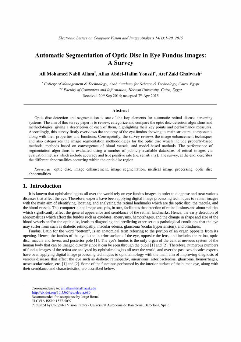
Figure 2 proposes the high-level system architecture of retinal image processing showing the data which is employed,
the steps which are followed and the procedures which are applied in processing the eye fundus images.
Each of the four components of the system architecture is briefly described below, and then discussed in detail in the
subsequent sections:
Input – retinal image datasets (section 4): refers to one set or more of retinal images that form the input data to be
processed.
Image processing (section 6): this is the backbone of the system architecture which is composed usually of three sub-
processes in order to manipulate the dataset of the raw retinal images and convert it to a set of meaningful images (e.g.
diagnosing a retinal image that suffers from a particular disease):
i. Preprocessing (section 6): a preliminary step that normally aims to enhancing the input image (e.g. contrast,
sharpness and illumination of the image).
ii. Retinal images processing (section 7): the main objective of processing the retinal image normally aims to the
segmentation of the image which is the process of isolating particular regions of interest within the image [6].
Regions of interest (ROI) may include retinal abnormalities (e.g. exudates, hemorrhages, aneurysms, etc.), and may
also include the retinal landmarks (e.g. optic disc, macula, and vascular tree) as discussed earlier at section 2.
iii. Post-processing: refers to the last processing step that aims to describing and marking (i.e. annotating) either the
external boundary or the internal skeleton of the objects/regions that were segmented in the fundus image.
Output – processed retinal images: the output dataset which refers to the retinal images after being enhanced, processed
and then annotated. These processed retina images are compared to the ground truth in order to evaluate the accuracy
of experimental work.
Evaluation (section 5): the accuracy of experimental results is measured by estimating indices for the true positive, true
negative, false positive, and false negative.
4. Retinal Image Datasets
The retinal images are considered as the raw material to be enhanced, segmented and evaluated. Image datasets are
normally accompanied with a ground truth which acts as a benchmark for comparing and evaluating the achieved
experimental results using the true results provided usually by medical experts (i.e. ophthalmologists) on an image dataset.
Table 1 shows a chronological list of the most widely used datasets of retinal images employed for optic disc image
processing, in particular.
Table 1. Retinal images datasets
Dataset Name Dataset Size FOV Image Size (pixels) Images
Format Ground Truth
STARE (2000) 397 images 35° 700 × 605 PPM Blood Vessels and Optic Disc
DRIVE (2004) 40 images (two sets) 45° 565 × 584 (both sets) TIFF Blood Vessels
MESSIDOR
(2004)
1200 images
(three sets) 45°
Set(1): 1440 × 960
Set(2): 2240 × 1488
Set(3): 2304 × 1536
TIFF Retinopathy Grading and
Macular Edema (Hard Exudates)
ONHSD (2004) 99 images 45° 760 × 570 BMP Optic Disc
ARIA (2006) 143 images (three sets) 50° 768 × 576 TIFF Vessels, Optic Disc and Fovea
ImageRet
(2008)
Diaretdb0: 130 images
Diaretdb1: 89 images
50° 1500 × 1152 PNG Microaneurysms, Hemorrhages,
and Hard & Soft Exudates
1. INPUT
Retinal
Image
Dataset(s)
2. IMAGE PROCESSING 3. OUTPUT
Retinal Images
Processing
4. EVALUATION
Processed
Retinal
Images
Measure
Sensitivity &
Specificity
Pre-processing
Post-processing
Figure 2. Architecture of retinal image processing
4 Allam et al. / Electronic Letters on Computer Vision and Image Analysis 14(1):1-20, 2015
There are other more publicly available databases, such as REVIEW, HRF and ROC, which are not described here as
they are not commonly used by researchers in optic disc segmentation, as noticed in section 7. A more detailed description
of the most widely used publicly available datasets described in the table above, along with an explanation of their ground
truth, is overviewed below:
4.1. STARE
Dataset description: STARE dataset (Structured Analysis of the Retina) [7] contains 397 raw images captured using a
fundus camera with a field of view (FOV) of 35 degrees. Each image is of size of 700×605 pixels, with 24 bits per pixel;
the images have been clipped at the top and the bottom of the FOV.
Ground truth: each image within the dataset is diagnosed as pertaining to one or more of thirteen different abnormalities,
in which blood vessel segmentation experimental work is provided including 40 hand-labeled images, along with the
experimental results, and a demo. Also optic disc detection work including 81 images is also provided along with ground
truth, and the experimental results.
4.2. DRIVE
Dataset description: DRIVE database (Digital Retinal Images for Vessel Extraction) [8] has been developed for
comparative studies on segmentation of blood vessels in retinal images. The dataset contains 40 images in which 33 do
not show any sign of diabetic retinopathy and 7 show signs of mild early diabetic retinopathy. Each image was captured
using 8 bits per color plane at 565×584 pixels with a FOV of 45 degrees. For this database, the images have been cropped
around the FOV, and for each image, a mask image is provided that delineates the FOV.
Ground truth: the set of 40 images has been divided into a training set and a test set, both containing 20 images. For the
training images, a single manual segmentation of the vasculature is available. For the test cases, two manual segmentations
are available; one is used as gold standard, the other one can be used to compare computer generated segmentations with
those of an independent human observer. The DRIVE’s website provides a results page that lists results from some
algorithms in a tabular format. The result browser is a useful way to explore the database by viewing images and
segmentations for a small set of methods that had been implemented.
4.3. MESSIDOR
Dataset description: MESSIDOR database (Méthodes d'Evaluation de Systèmes de Segmentation et
d'Indexation Dédiées à l'Ophtalmologie Rétinienne) [9] has been established to facilitate studies on computer-assisted
diagnoses of diabetic retinopathy. The dataset contains 1200 images packaged in three sets. Each set is divided into four
subsets, each of which containing 100 images in TIFF format. The images were captured acquired using a camera with a
45 degree field of view using 8 bits per color plane at 1440×960, 2240×1488 and 2304×1536 pixels.800 images were
acquired with pupil dilation (one drop of Tropicamide at 0.5%) and 400 without dilation.
Ground truth: each set is associated with a spreadsheet that includes two diagnoses which are the retinopathy grade and
the risk grade of macular edema provided by medical experts for each image. The retinopathy grade is classified into four
grades (grade 0, 1, 2 and 3) according to three main factors which are the number of microaneurysms, number of
hemorrhages, and the neovascularization. On the other hand, hard exudates have been used to classify the risk of macular
edema into three grades (grade 0, 1 and 2).
4.4. ONHSD
Dataset description: ONHSD dataset (Optic Nerve Head Segmentation Dataset) [10] contains 99 fundus images taken
from 50 patients randomly sampled from a diabetic retinopathy screening program; 96 images have discernible Optic
Nerve Head (ONH).The images were acquired using a fundus camera with a field angle lens of 45 degrees and size of
760×570 pixels. Images were converted to gray-scale by extracting the intensity component from the HSI representation.
There is considerable quality variation in the images, with many characteristics that can affect segmentation algorithms.
Ground truth: the ONH center has been marked up by a clinician. Then, four clinicians marked the ONH edge where it
intersects with radial spokes (at 15 degree angles) radiating from the nominated center. These multiple nominations of
the edge are used to characterize the degree of subjective uncertainty in the edge position.
4.5. ARIA
Dataset description: ARIA (Automated Retinal Image Analysis) [11], [12] aims to provide an automated image capture
and image analysis platform capable of predicting individuals at risk of eye disease. The dataset contains a total of 143
images collected by staff members of St. Paul's Eye Unit and the University of Liverpool as part of the ARIA project.
The images are captured with a camera of FOV of 50 degrees at resolution of 768×576 and stored as uncompressed TIFF
files. The dataset is organized into three groups, including23 images of age-related macular degeneration, 61 images
healthy control-group, and 59 diabetic images.
Ground truth: Two image analysis experts have traced out the blood vessels in the images of all three groups. Also, the
locations of the optic disk and fovea have also been outlined in the diabetic and healthy control groups.
Allam et al. / Electronic Letters on Computer Vision and Image Analysis 14(1):1-20, 2015 5
4.6. ImageRet
Dataset Description: ImageRet database [13] is divided into two subsets, DIARETDB0 and DIARETDB1, which are
used for benchmarking diabetic retinopathy detection. The ImageRet dataset was made publicly available in 2008 using
a digital fundus camera of 50 degrees field of view in which each image is of size of 1500×1152 pixels in PNG format.
The DIARETDB0 subset contains 130 retinal images of which 20 are normal and the other 110 images contain various
symptoms of diabetic retinopathy, whereas DIARETDB1 contains 89 color fundus images of which 84 contain at least
mild non-proliferative signs (i.e. microaneurysms) of the diabetic retinopathy, and 5 are considered as normal which do
not contain any signs of the diabetic retinopathy.
Ground truth: For every fundus image there is a corresponding ground truth file. A ground truth file contains all finding
types found in the specific image, namely, red small dots (i.e. microaneurysms), hemorrhages, hard exudates, soft
exudates, and neovascularization.
5. Evaluation Metrics
Although the evaluation of an algorithm normally comes at the final stage of a detection and segmentation method, yet
the metrics used for evaluation are reviewed here in advance, in order to provide a concrete understanding of the results
achieved by the segmentation algorithms in the literature which will be reviewed consequently in section 7.
In medical diagnosis, the region of interest ROI (i.e. landmark or lesion) is usually classified into two classes: present
or absent; in which the response given by a human observer (expert) or a computer process is: positive or negative.
Therefore, the detection of the ROI is normally depicted using the terms presented in Table 2 [14]. The evaluation of the
medical imaging test is usually determined by estimating indexes for the true positive (TP), true negative (TN), false
positive (FP), false negative (FN).
Table 2. Signal detection indices and derived evaluation metrics
Present ROI Absent ROI
Positive Response Hit (TP) False alarm (FP)
Negative Response Miss (FN) Correct rejection (TN)
SENS= 𝐓𝐏
𝐓𝐏+𝐅𝐍 SPEC=
𝐓𝐍
𝐓𝐍+𝐅𝐏
The TP and TN indices refer to the successful response in detecting and rejecting region of interests, respectively. The
true positive index (TP) indicates the positive response of a human observer or computer for the ROI that is present within
the retina, while the true negative index (TN) indicates the negative response for a landmark or abnormality that is not
present. On the other hand, the FP and FN indices refer to an unsuccessful rejection and detection, respectively. The false
positive index (FP) indicates the positive response for the ROI that is not present, whereas the false negative index (FN)
indicates the negative response for the ROI that is present.
Derived from the four aforementioned indices as shown in Table 2, four statistical metrics are computed in order to
evaluate the detection of landmarks or abnormalities, which are: sensitivity, specificity, positive predictive value, and
negative predictive value.
5.1. Sensitivity and Specificity
Sensitivity is a measure that reflects the probability of a positive response for the cases in which the landmark or
abnormality is present, whereas specificity is the probability of negative response for the cases in which the landmark or
abnormality is absent. Both, sensitivity and specificity are expressed either as a proportion or a percentage given by the
equation shown in Table 2, in which sensitivity and specificity are sometimes referred to as true positive rate and true
negative rate, respectively. Moreover, the term false positive rate (FPR) is also used for the complement of specificity,
computed as (1 − specificity) [15].
5.2. Segmentation Accuracy
Normally, the spatial features of an object of interest such as its size, shape and area are the parameters that are
commonly used in order to evaluate the segmentation accuracy of an object of interest. Moreover, these parameters also
have clinical significance because they help in diagnosing and treating diseases, as well as assessing the effect of
treatment. Therefore, the main requirement needed to evaluate the segmentation results is the presence of the ground truth
which is manually-defined by human observers indicating the true features of the segmented object (i.e. its true size,
shape or area). Thus, once the ground truth data is available, a variety of metrics can be used to evaluate the segmentation
process. These evaluation metrics include the Hausdorff distance and the degree of overlap, which are relatively easy to
compute and at the same time are not limited to certain geometrical patterns [16]. Other pixel-wise metrics such as the
6 Allam et al. / Electronic Letters on Computer Vision and Image Analysis 14(1):1-20, 2015
Euclidean distance is sometimes used to measure similarity, but the main drawback of such metric is that the similarity is
estimated according to the distance between only two pixels such as the distance between the centroid of two optic discs.
Hausdorff Distance
The intuition behind Hausdorff distance is to measure the similarity between two sets. So, if these sets have close
Hausdorff distance, they are considered to look almost the same. Therefore, the Hausdorff distance h(A,B) is used to
measure the similarity between two contours of the same object (e.g. optic disc), in which one contour A is defined by a
human expert while the other contour B is generated by a computer process. The Hausdorff distance is computed as
follows [16], [17]:
Let A = {a1, a2, ... am} and B = { b1, b2, ... bm} be the set of points on the two contours in which each point represents a
pair of x and y coordinates. Then, the distance of a point ai to the closest point on curve B is defined as
𝒅(𝒂𝒊, 𝑩) = 𝐦𝐢𝐧𝒋
‖𝒃𝒋 − 𝒂𝒊‖ (1)
Similarly, the distance of a point bj to the closest point on curve A is given by
𝒅(𝒃𝒋, 𝑨) = 𝐦𝐢𝐧𝒊
‖𝒂𝒊 − 𝒃𝒋‖ (2)
Finally, the Hausdorff distance is defined as the maximum of the above distances between the two contours.
𝒉(𝑨, 𝑩) = 𝐦𝐚𝐱 [𝐦𝐚𝐱𝒊
{𝒅(𝒂𝒊, 𝑩)} , 𝐦𝐚𝐱 𝒋
{𝒅(𝒃𝒋, 𝑨)}] (3)
Overlap Score
The degree of overlap between two areas G and E encompassed by contours A and B, respectively, is defined as the
ratio of the intersection and the union of these two areas, where G is the ground truth human-defined area and E is the
experimental computer-generated area. The degree of overlap is computed as follows [16], [18], [19]:
𝑶𝑳 = 𝑮 ∩ 𝑬
𝑮 ∪ 𝑬 (4)
If there is an exact overlap between both contours, the ratio will be 1, whereas the ratio is given by 0 if there is no
overlap between the two contours.
6. Preprocessing Functions: Image Enhancement
As mentioned before, image processing is the main component of the system architecture which includes three sub-
processes in order to manipulate the dataset of the captured retinal images and convert it to a set of meaningful images.
The input image is first enhanced, then segmented, and finally annotated. Software packages such as MATLAB® and
ImageJ® provide a powerful means for implementing these image processing functions.
Unfortunately, the raw digital fundus images are not always ready for immediate processing because of their poor
quality due to factors such as the patient’s movement and iris color, as well as imaging conditions such as non-uniform
illumination. Therefore, an image should be first preprocessed in order to make it more suitable for further processing.
The following subsections present the main preprocessing functions.
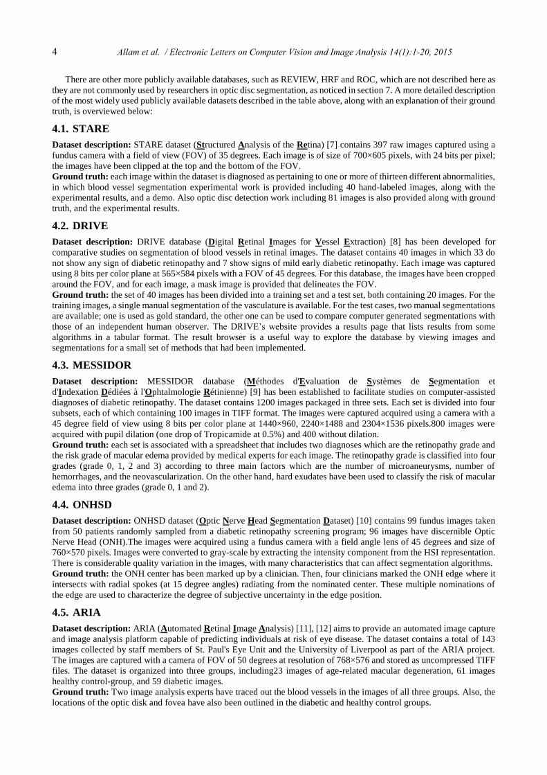
6.1. Mask Generation
A fundus image consists of a semi-oval region of interest (ROI) on a dark background which is never really pure black
(i.e. non-zero intensity). Therefore, masks are created and used in order to exclude the dark background of the image from
further calculations and processing; in other words, only the pixels belonging to the semi-oval retinal fundus are included
for processing. The mask image is a binary image in which the background pixels are assigned the value of “zero” and
pixels within the ROI are assigned the value of “one”, where the original color image is multiplied by the created mask
image to produce a color image without noisy pixels in the background, while the ROI is left unchanged [20], as shown
in Figure 3.
(a) (c) (b)
Figure 3. Mask generation
(a) A color image, (b) its corresponding mask, and (c) its excluded background
Allam et al. / Electronic Letters on Computer Vision and Image Analysis 14(1):1-20, 2015 7
However, some of the publicly available retinal datasets, such as DRIVE, HRF, DIARETDB0 and DIARETDB1, are
accompanied with the corresponding mask images, but most of the other datasets do not include such mask images, and
therefore the retinal images must be manipulated in some way in order to generate their corresponding masks.
For instance, in their procedure of detecting the anatomical structures in fundus images, Gagnon et al. [21] generated
the mask image using pixel value statistics outside the ROI of the fundus image which were calculated for each of the
three color bands. Consequently, a 4-sigma thresholding was applied such that pixels with intensity value above that
threshold were considered to belong to the ROI. Finally, results for all bands were combined through logical operations
and region connectivity test in order to identify the largest common connected mask, since ROI size was not always the
same for each band due to different color response of the camera.
Also, Goatman et al. [22] automatically generated the masks by the simple thresholding of the green channel of the
retinal image followed by a 5×5 median filtering in order to exclude the dark surrounding region.
Ter Haar [20] created the mask by thresholding the red channel of the retinal image using a threshold value that was
determined empirically, and then the thresholded image was morphologically processed via the opening, closing and
erosion operators through a 3×3 square kernel.
In the same direction, Hashim et al. [23] generated the binary mask by convolving the red channel with a Gaussian
low-pass filter, in which the resultant image was thresholded using Otsu’s global threshold.
6.2. Color Channels Processing
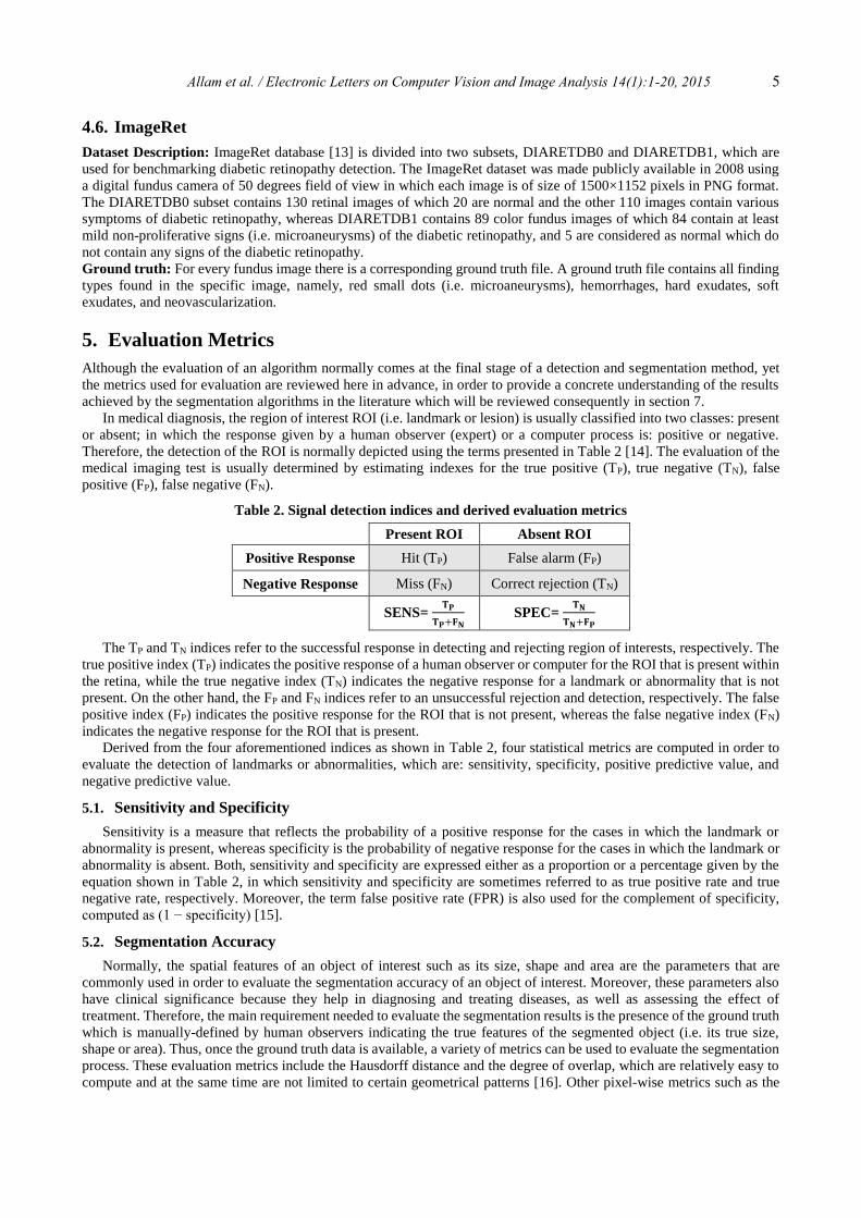
The retinal fundus color image consists of three channels, in which the green channel has the highest contrast, whereas
the red channel tends to be saturated and it is the brightest channel, while the blue channel tends to be empty [24], as
shown in Figure 4.
Because it provides the highest contrast, the green channel has been extensively exploited by most algorithms,
discarding the red component in some cases “so-called red-free images” and ignoring the blue component in most, or
even all, algorithms. Therefore, the green channel was utilized for miscellaneous purposes such as detecting different
retinal landmarks and several abnormalities due to its high contrast within retinal images. For instance, Hoover and
Goldbaum [24] located the optic disc using only the green band of the retinal image, whereas Staal et al. [8] used the
green channel for the extraction of image ridges in color fundus images, while Niemeijer et al. [25] localized both the
optic disc and fovea simultaneously using only the green plane of the color fundus image.
However, even though the green channel was utilized solely in most approaches and for different purposes as
mentioned in the previous paragraph, yet the red channel was also exploited sometimes in combination with the green
band. For instance, Aquino et al. [19] observed that the optic disc appeared in the red field as a well-defined white shape,
brighter than the surrounding area, and therefore, the optic disc segmentation was performed in parallel on the red and
green bands and the better of the two segmentations was ultimately selected. Also, Lu [18] and Hashim et al. [23]
combined intensity information from the red and green channels together by calculating a modified intensity channel
component using a weighted average, in which a higher weight was given to the red channel in order to keep the image
variation across the optic disc boundary but suppress that across the retinal vessels.
6.3. Color Normalization
Another major preprocessing task in retinal images is color normalization which does not aim to find the true color of
an image, but in fact color normalization algorithms transform the color of an image so as to be invariant with respect to
the color of illumination, without losing the ability to differentiate between the objects or regions of interest [22]. The
most frequently-used algorithms for color normalization are the gray-world normalization, comprehensive normalization,
histogram equalization and histogram specification.
Gray-world normalization, also referred to as gray-world assumption algorithm, assumes that the changes in the
illuminating spectrum can be modeled by three multiplicative constants applied to the red, green and blue channels,
respectively. The new color of any pixel is calculated by dividing each color channel by its respective mean value,
removing the dependence on the multiplicative constant. Comprehensive normalization, a variation of the gray-world
normalization proposed by Finlayson et al. [26], is a technique that iteratively applies chromaticity normalization followed
by gray-world normalization for four or five iterations, until the change in values is less than a certain tolerance value.
(a) (c) (b) (d)
Figure 4. (a) Full-color image split into its (b) RED, (c) GREEN and (d) BLUE channels
8 Allam et al. / Electronic Letters on Computer Vision and Image Analysis 14(1):1-20, 2015
On the other hand, histogram equalization is a non-linear transform applied individually to the red, green and blue
bands of an image which affects the color perceived. It is considered to be a more powerful normalization transformation
than the gray-world method. The results of histogram equalization tend to have an exaggerated blue channel and look
unnatural due to the fact that in most images the distribution of the pixel values is usually more similar to a Gaussian
distribution, rather than uniform [27].
Last but not least, histogram specification transforms the red, green and blue histograms to match the shapes of three
specific histograms, rather than simply equalizing them, which results in more realistic images than those produced by
equalization [22].
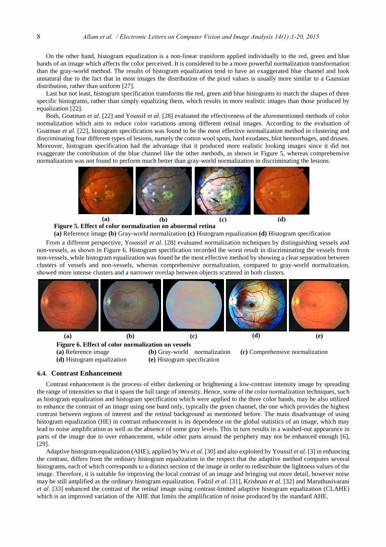
Both, Goatman et al. [22] and Youssif et al. [28] evaluated the effectiveness of the aforementioned methods of color
normalization which aim to reduce color variations among different retinal images. According to the evaluation of
Goatman et al. [22], histogram specification was found to be the most effective normalization method in clustering and
discriminating four different types of lesions, namely the cotton wool spots, hard exudates, blot hemorrhages, and drusen.
Moreover, histogram specification had the advantage that it produced more realistic looking images since it did not
exaggerate the contribution of the blue channel like the other methods, as shown in Figure 5, whereas comprehensive
normalization was not found to perform much better than gray-world normalization in discriminating the lesions.
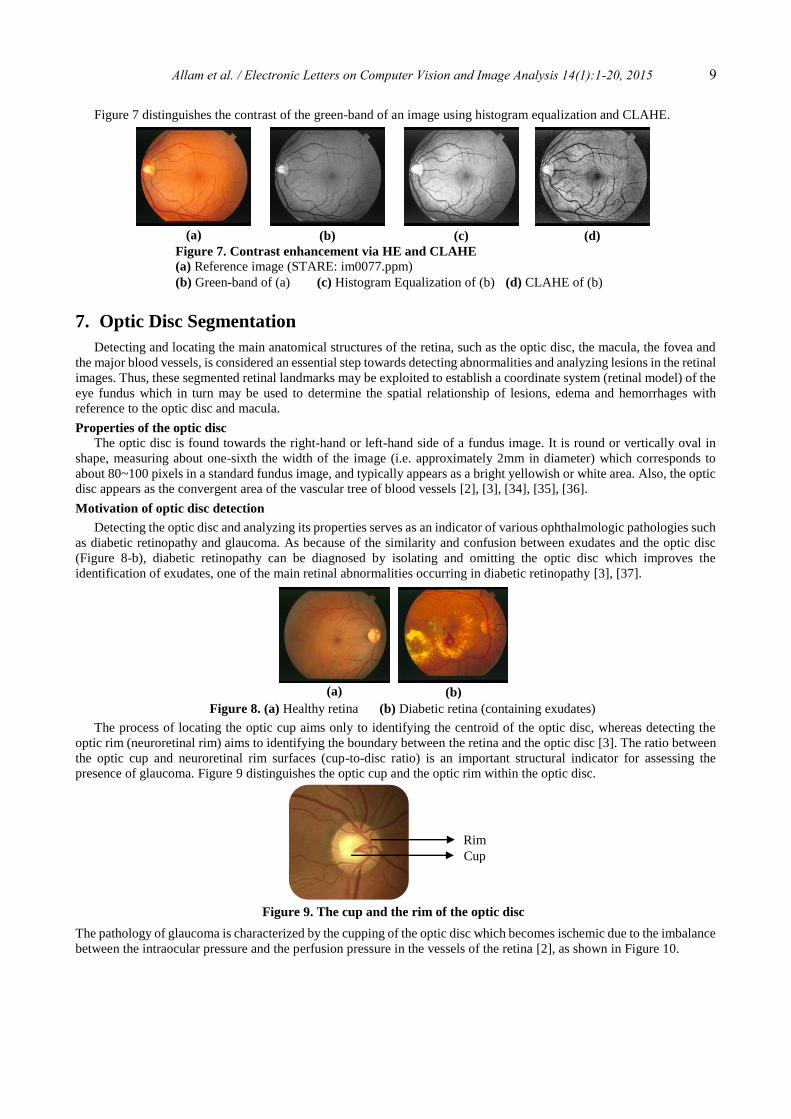
From a different perspective, Yousssif et al. [28] evaluated normalization techniques by distinguishing vessels and
non-vessels, as shown in Figure 6. Histogram specification recorded the worst result in discriminating the vessels from
non-vessels, while histogram equalization was found be the most effective method by showing a clear separation between
clusters of vessels and non-vessels, whereas comprehensive normalization, compared to gray-world normalization,
showed more intense clusters and a narrower overlap between objects scattered in both clusters.
6.4. Contrast Enhancement
Contrast enhancement is the process of either darkening or brightening a low-contrast intensity image by spreading
the range of intensities so that it spans the full range of intensity. Hence, some of the color normalization techniques, such
as histogram equalization and histogram specification which were applied to the three color bands, may be also utilized
to enhance the contrast of an image using one band only, typically the green channel, the one which provides the highest
contrast between regions of interest and the retinal background as mentioned before. The main disadvantage of using
histogram equalization (HE) in contrast enhancement is its dependence on the global statistics of an image, which may
lead to noise amplification as well as the absence of some gray levels. This in turn results in a washed-out appearance in
parts of the image due to over enhancement, while other parts around the periphery may not be enhanced enough [6],
[29].
Adaptive histogram equalization (AHE), applied by Wu et al. [30] and also exploited by Youssif et al. [3] in enhancing
the contrast, differs from the ordinary histogram equalization in the respect that the adaptive method computes several
histograms, each of which corresponds to a distinct section of the image in order to redistribute the lightness values of the
image. Therefore, it is suitable for improving the local contrast of an image and bringing out more detail, however noise
may be still amplified as the ordinary histogram equalization. Fadzil et al. [31], Krishnan et al. [32] and Maruthusivarani
et al. [33] enhanced the contrast of the retinal image using contrast-limited adaptive histogram equalization (CLAHE)
which is an improved variation of the AHE that limits the amplification of noise produced by the standard AHE.
(a) (b) (c) (d) Figure 5. Effect of color normalization on abnormal retina
(a) Reference image (b) Gray-world normalization (c) Histogram equalization (d) Histogram specification
(a) (b) (c) (d) (e)
Figure 6. Effect of color normalization on vessels
(a) Reference image (b) Gray-world normalization (c) Comprehensive normalization
(d) Histogram equalization (e) Histogram specification
Allam et al. / Electronic Letters on Computer Vision and Image Analysis 14(1):1-20, 2015 9
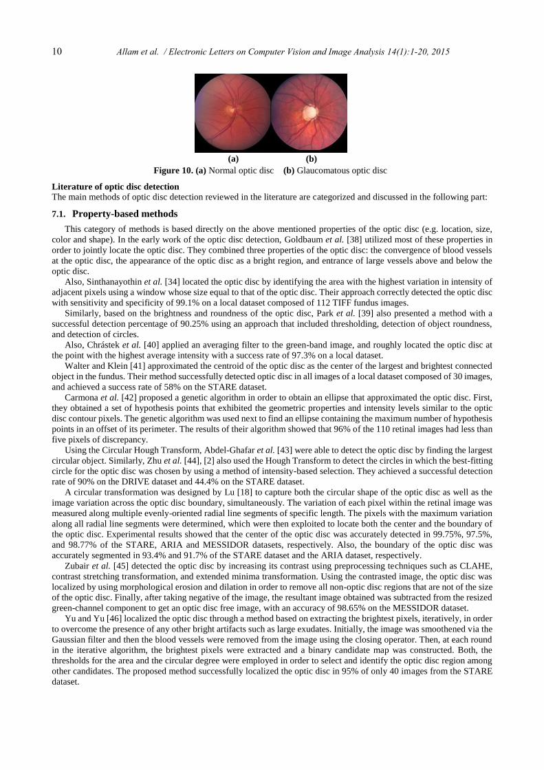
Figure 7 distinguishes the contrast of the green-band of an image using histogram equalization and CLAHE.
7. Optic Disc Segmentation
Detecting and locating the main anatomical structures of the retina, such as the optic disc, the macula, the fovea and
the major blood vessels, is considered an essential step towards detecting abnormalities and analyzing lesions in the retinal
images. Thus, these segmented retinal landmarks may be exploited to establish a coordinate system (retinal model) of the
eye fundus which in turn may be used to determine the spatial relationship of lesions, edema and hemorrhages with
reference to the optic disc and macula.
Properties of the optic disc
The optic disc is found towards the right-hand or left-hand side of a fundus image. It is round or vertically oval in
shape, measuring about one-sixth the width of the image (i.e. approximately 2mm in diameter) which corresponds to
about 80~100 pixels in a standard fundus image, and typically appears as a bright yellowish or white area. Also, the optic
disc appears as the convergent area of the vascular tree of blood vessels [2], [3], [34], [35], [36].
Motivation of optic disc detection
Detecting the optic disc and analyzing its properties serves as an indicator of various ophthalmologic pathologies such
as diabetic retinopathy and glaucoma. As because of the similarity and confusion between exudates and the optic disc
(Figure 8-b), diabetic retinopathy can be diagnosed by isolating and omitting the optic disc which improves the
identification of exudates, one of the main retinal abnormalities occurring in diabetic retinopathy [3], [37].
The process of locating the optic cup aims only to identifying the centroid of the optic disc, whereas detecting the
optic rim (neuroretinal rim) aims to identifying the boundary between the retina and the optic disc [3]. The ratio between
the optic cup and neuroretinal rim surfaces (cup-to-disc ratio) is an important structural indicator for assessing the
presence of glaucoma. Figure 9 distinguishes the optic cup and the optic rim within the optic disc.
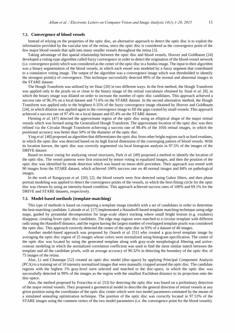
The pathology of glaucoma is characterized by the cupping of the optic disc which becomes ischemic due to the imbalance
between the intraocular pressure and the perfusion pressure in the vessels of the retina [2], as shown in Figure 10.
(a) (b) (c) (d)
Figure 7. Contrast enhancement via HE and CLAHE
(a) Reference image (STARE: im0077.ppm)
(b) Green-band of (a) (c) Histogram Equalization of (b) (d) CLAHE of (b)
(a) (b)
Figure 8. (a) Healthy retina (b) Diabetic retina (containing exudates)
Rim
Cup
Figure 9. The cup and the rim of the optic disc
10 Allam et al. / Electronic Letters on Computer Vision and Image Analysis 14(1):1-20, 2015
Literature of optic disc detection The main methods of optic disc detection reviewed in the literature are categorized and discussed in the following part:
7.1. Property-based methods
This category of methods is based directly on the above mentioned properties of the optic disc (e.g. location, size,
color and shape). In the early work of the optic disc detection, Goldbaum et al. [38] utilized most of these properties in
order to jointly locate the optic disc. They combined three properties of the optic disc: the convergence of blood vessels
at the optic disc, the appearance of the optic disc as a bright region, and entrance of large vessels above and below the
optic disc.
Also, Sinthanayothin et al. [34] located the optic disc by identifying the area with the highest variation in intensity of
adjacent pixels using a window whose size equal to that of the optic disc. Their approach correctly detected the optic disc
with sensitivity and specificity of 99.1% on a local dataset composed of 112 TIFF fundus images.
Similarly, based on the brightness and roundness of the optic disc, Park et al. [39] also presented a method with a
successful detection percentage of 90.25% using an approach that included thresholding, detection of object roundness,
and detection of circles.
Also, Chrástek et al. [40] applied an averaging filter to the green-band image, and roughly located the optic disc at
the point with the highest average intensity with a success rate of 97.3% on a local dataset.
Walter and Klein [41] approximated the centroid of the optic disc as the center of the largest and brightest connected
object in the fundus. Their method successfully detected optic disc in all images of a local dataset composed of 30 images,
and achieved a success rate of 58% on the STARE dataset.
Carmona et al. [42] proposed a genetic algorithm in order to obtain an ellipse that approximated the optic disc. First,
they obtained a set of hypothesis points that exhibited the geometric properties and intensity levels similar to the optic
disc contour pixels. The genetic algorithm was used next to find an ellipse containing the maximum number of hypothesis
points in an offset of its perimeter. The results of their algorithm showed that 96% of the 110 retinal images had less than
five pixels of discrepancy.
Using the Circular Hough Transform, Abdel-Ghafar et al. [43] were able to detect the optic disc by finding the largest
circular object. Similarly, Zhu et al. [44], [2] also used the Hough Transform to detect the circles in which the best-fitting
circle for the optic disc was chosen by using a method of intensity-based selection. They achieved a successful detection
rate of 90% on the DRIVE dataset and 44.4% on the STARE dataset.
A circular transformation was designed by Lu [18] to capture both the circular shape of the optic disc as well as the
image variation across the optic disc boundary, simultaneously. The variation of each pixel within the retinal image was
measured along multiple evenly-oriented radial line segments of specific length. The pixels with the maximum variation
along all radial line segments were determined, which were then exploited to locate both the center and the boundary of
the optic disc. Experimental results showed that the center of the optic disc was accurately detected in 99.75%, 97.5%,
and 98.77% of the STARE, ARIA and MESSIDOR datasets, respectively. Also, the boundary of the optic disc was
accurately segmented in 93.4% and 91.7% of the STARE dataset and the ARIA dataset, respectively.
Zubair et al. [45] detected the optic disc by increasing its contrast using preprocessing techniques such as CLAHE,
contrast stretching transformation, and extended minima transformation. Using the contrasted image, the optic disc was
localized by using morphological erosion and dilation in order to remove all non-optic disc regions that are not of the size
of the optic disc. Finally, after taking negative of the image, the resultant image obtained was subtracted from the resized
green-channel component to get an optic disc free image, with an accuracy of 98.65% on the MESSIDOR dataset.
Yu and Yu [46] localized the optic disc through a method based on extracting the brightest pixels, iteratively, in order
to overcome the presence of any other bright artifacts such as large exudates. Initially, the image was smoothened via the
Gaussian filter and then the blood vessels were removed from the image using the closing operator. Then, at each round
in the iterative algorithm, the brightest pixels were extracted and a binary candidate map was constructed. Both, the
thresholds for the area and the circular degree were employed in order to select and identify the optic disc region among
other candidates. The proposed method successfully localized the optic disc in 95% of only 40 images from the STARE
dataset.
(a) (b)
Figure 10. (a) Normal optic disc (b) Glaucomatous optic disc
Allam et al. / Electronic Letters on Computer Vision and Image Analysis 14(1):1-20, 2015 11
7.2. Convergence of blood vessels
Instead of relying on the properties of the optic disc, an alternative approach to detect the optic disc is to exploit the
information provided by the vascular tree of the retina, since the optic disc is considered as the convergence point of the
few major blood vessels that split into many smaller vessels throughout the retina [3].
Taking advantage of this spatial relationship between the optic disc and blood vessels, Hoover and Goldbaum [24]
developed a voting-type algorithm called fuzzy convergence in order to detect the origination of the blood-vessel network
(i.e. convergence point) which was considered as the center of the optic disc in a fundus image. The input to their algorithm
was a binary segmentation of the blood vessels, in which each vessel was modeled by a fuzzy segment that contributed
to a cumulative voting image. The output of the algorithm was a convergence image which was thresholded to identify
the strongest point(s) of convergence. This technique successfully detected 89% of the normal and abnormal images in
the STARE dataset.
The Hough Transform was utilized by ter Haar [20] in two different ways. In the first method, the Hough Transform
was applied only to the pixels on or close to the binary image of the retinal vasculature obtained by Staal et al. [8], in
which the binary image was dilated on order to increase the number of optic disc candidates. This approach achieved a
success rate of 96.3% on a local dataset and 71.6% on the STARE dataset. In the second alternative method, the Hough
Transform was applied only to the brightest 0.35% of the fuzzy convergence image obtained by Hoover and Goldbaum
[24], in which dilation was applied again to the convergence image to fill the gaps created by small vessels. This approach
achieved a success rate of 97.4% on a local dataset and 65.4% on the STARE dataset.
Fleming et al. [47] detected the approximate region of the optic disc using an elliptical shape of the major retinal
vessels which was formed using the Generalized Hough Transform. The approximate location of the optic disc was then
refined via the Circular Hough Transform achieving a success rate of 98.4% of the 1056 retinal images, in which the
positional accuracy was better than 50% of the diameter of the optic disc.
Ying et al. [48] proposed an algorithm that differentiates the optic disc from other bright regions such as hard exudates,
in which the optic disc was detected based on its high fractal dimension of the converging pattern of blood vessels. With
its location known, the optic disc was correctly segmented via local histogram analysis in 97.5% of the images of the
DRIVE dataset.
Based on tensor voting for analyzing vessel structures, Park et al. [49] proposed a method to identify the location of
the optic disc. The vessel patterns were first extracted by tensor voting in equalized images, and then the position of the
optic disc was identified by mode detection which was based on mean-shift procedure. Their approach was tested with
90 images from the STARE dataset, which achieved 100% success rate on 40 normal images and 84% on pathological
images.
In the work of Rangayyan et al. [50], [2], the blood vessels were first detected using Gabor filters, and then phase
portrait modeling was applied to detect the convergence points of the vessels, in which the best-fitting circle for the optic
disc was chosen by using an intensity-based condition. This approach achieved success rates of 100% and 69.1% for the
DRIVE and STARE datasets, respectively.
7.3. Model-based methods (template-matching)
This type of methods is based on comparing a template image (model) with a set of candidates in order to determine
the best-matching candidate. Lalonde et al. [17] implemented a Hausdorff-based template matching technique using edge
maps, guided by pyramidal decomposition for large-scale object tracking where small bright lesions (e.g. exudates)
disappear, creating fewer optic disc candidates. The edge map regions were matched to a circular template with different
radii using the Hausdorff distance, and the region having the largest number of overlapped template pixels was considered
the optic disc. This approach correctly detected the center of the optic disc in 93% of a dataset of 40 images.
Another model-based approach was proposed by Osareh et al. [51] who created a gray-level template image by
averaging the optic disc region of 25 images whose colors were normalized using histogram specification. The center of
the optic disc was located by using the generated template along with gray-scale morphological filtering and active-
contour modeling in which the normalized correlation coefficient was used to find the most similar match between the
template and all the candidate pixels, with an average accuracy of 90.32% in detecting the boundary of the optic disc of
75 images of the retina.
Also, Li and Chutatape [52] created an optic disc model (disc-space) by applying Principal Component Analysis
(PCA) to a training set of 10 intensity normalized images that were manually cropped around the optic disc. The candidate
regions with the highest 1% gray-level were selected and matched to the disc-space, in which the optic disc was
successfully detected in 99% of the images as the region with the smallest Euclidean distance to its projection onto the
disc-space.
Also, the method proposed by Foracchia et al. [53] for detecting the optic disc was based on a preliminary detection
of the major retinal vessels. They proposed a geometrical model to describe the general direction of retinal vessels at any
given position using the coordinates of the optic disc center which were two model parameters estimated by the means of
a simulated annealing optimization technique. The position of the optic disc was correctly located in 97.53% of the
STARE images using the common vertex of the two model parameters (i.e. the convergence point for the blood vessels).
12 Allam et al. / Electronic Letters on Computer Vision and Image Analysis 14(1):1-20, 2015
Lowell et al. [10] designed a detection filter (i.e. template) for the optic disc which was composed of a Laplacian of
Gaussian filter with a vertical channel carved out of the middle corresponding to the major blood vessels exiting the optic
disc vertically. This template was then correlated to the intensity component of the fundus image using full Pearson-R
correlation. The optic disc was successfully detected in 99% of the images in a local dataset.
A method presented by ter Haar [20] was based on fitting the vascular orientations on a directional model (DM), using
a training set of 80 images of vessel segmentations. For all the pixels in each vessels image, the orientation was calculated
to form a directional vessel map, in which the DM was created by averaging, at each pixel, all the corresponding
orientation values in the directional maps. At the end, each pixel in an input vasculature was aligned to the center of the
optic disc, and the pixel having the minimal distance to both DMs was selected as the optic disc location. This method
detected the optic disc successfully in 99.5% of the images in a local dataset and 93.8% of the STARE dataset.
Closely related, Youssif et al. [3] proposed another model-based approach by matching the expected directional
pattern of the retinal blood vessels found in the vicinity of the optic disc. They obtained a vessels direction map of the
retinal vessels that were segmented using 2D Gaussian matched filter. The minimum difference between the matched
filter and the vessels directions at the surrounding area of each of the optic disc candidates achieved a successful detection
rate of 100% on the DRIVE dataset and 98.77% on the STARE dataset.
Niemeijer et al. [25] formulated the problem of finding a certain position in a retinal image as a regression problem.
A k-nearest neighbor classifier (k-NN) was trained to predict the distance to the optic disc given a set of measurements
of the retinal vasculature obtained around a circular template placed at a certain location in the image. The method was
trained with 500 images for which the location of the optic disc was known, where the point with the lowest predicted
distance to the optic disc was selected as the optic disc center. This supervised method was tested using 600 images of
which 100 images contained gross abnormalities, and successfully located the optic disc in 99.4% of the normal images
and 93% of the pathological images.
Aquino et al. [19] presented a template-based methodology that used morphological and edge detection techniques
followed by the Circular Hough Transform to obtain an approximate circular optic disc boundary. Their methodology
required an initial pixel located within the optic disc, and for this purpose, a location procedure based on a voting-type
algorithm was utilized and succeeded in 99% of the cases. The algorithms were evaluated on the 1200 images of the
MESSIDOR dataset, achieving a success rate of 86%.
Lu [54] used another technique for the detection of the optic disc in a way different than the one he used in [18]
(previously reviewed in the section 7.1). In the proposed technique, the retinal background surface was first estimated
through an iterative Savitzky-Golay smoothing procedure. Afterwards, multiple optic disc candidates were detected
through the difference between the retinal image and the estimated retinal background surface. Finally, the real optic disc
was selected through the combination of the difference image and the directional retinal blood vessel which was based
on the observation that the retinal blood vessels were mostly oriented vertically as they exit the optic disc. The proposed
technique was evaluated over four datasets DIARETDB0, DIARETDB1, DRIVE and STARE giving an accuracy of
98.88%, 99.23%, 97.50% and 95.06%, respectively.
Instead of creating an image and using it as a template, Dehghani et al. [35] constructed three histograms as a template
for localizing the center of the optic disc using four retinal images from the DRIVE dataset, in which each histogram
represented one color channel. Then, an 80×80 window was moved through the retinal image to obtain the histogram of
each channel. Finally, they calculated the correlation between the histogram of each channel in the moving window and
the histograms of its corresponding channel in the template. The DRIVE, STARE, and a local dataset composed of 273
images were used to evaluate their proposed algorithm, in which the success rate was 100%, 91.36% and 98.9%,
respectively.
Lately, [55] proposed a method for detecting the optic disc accurately in an efficient way. First, the algorithm identified
a number of possible vertical windows (x-coordinates) for the optic disc according to three characteristics of retinal
vessels, which are: (1) the high density of vessels at optic disc vicinity, (2) compactness of the vertical vascular segments
around the optic disc center, and (3) the uniform distribution of vessels. Consequently, the y-coordinate of the optic disc
is identified according to the vessels direction via parabola curve fitting using the General Hough Transform. The
proposed method was tested on four datasets: DIARETDB0, DIARETDB1, DRIVE and STARE, in which the optic disc
was correctly detected in all images of each dataset, except only one image in the STARE dataset.
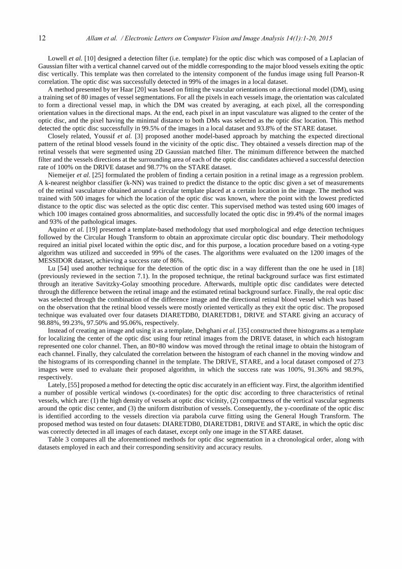
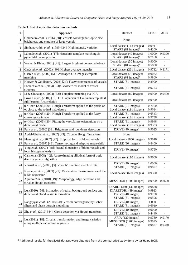
Table 3 compares all the aforementioned methods for optic disc segmentation in a chronological order, along with
datasets employed in each and their corresponding sensitivity and accuracy results.
Allam et al. / Electronic Letters on Computer Vision and Image Analysis 14(1):1-20, 2015 13
Table 3. List of optic disc detection methods
# Approach Dataset SENS ACC
1 Goldbaum et al., (1996) [38]: Vessels convergence, optic disc
brightness, and entrance of large vessels None - -
2 Sinthanayothin et al., (1999) [34]: High intensity variation Local dataset (112 images)
STARE (81 images)1
0.9911
0.4200
-
-
3 Lalonde et al., (2001) [17]: Hausdorff template matching &
pyramidal decomposition
Local dataset (40 images)
STARE (81 images)1
1.0000
0.7160
0.9300
-
4 Walter & Klein, (2001) [41]: Largest brightest connected object Local dataset (30 images)
STARE (81 images)1
0.9000
0.5800
-
-
5 Chrástek et al., (2002) [40]: Highest average intensity Local dataset (261 images) 0.9732 0.8171
6 Osareh et al., (2002) [51]: Averaged OD-images template
matching
Local dataset (75 images)
STARE (81 images)1
0.9032
0.5800
-
-
7 Hoover & Goldbaum, (2003) [24]: Fuzzy convergence of vessels STARE (81 images) 0.8900 -
8 Foracchia et al., (2004) [53]: Geometrical model of vessel
structure STARE (81 images) 0.9753 -
9 Li & Chutatape, (2004) [52]: Template matching via PCA Local dataset (89 images) 0.9900 0.9400
10 Lowell et al., (2004) [10]: OD Laplacian of Gaussian template &
full Pearson-R correlation Local dataset (90 images) 0.9900 -
11 ter Haar, (2005) [20]: Hough Transform applied to the pixels on
or close to the retinal vasculature
STARE (81 images)
Local dataset (191 images)
0.7160
0.9634
-
-
12 ter Haar, (2005) [20]: Hough Transform applied to the fuzzy
convergence image
STARE (81 images)
Local dataset (191 images)
0.6543
0.9738
-
-
13 ter Haar, (2005) [20]: Fitting the vasculature orientations on a
directional model
STARE (81 images)
Local dataset (191 images)
0.9948
0.9383
-
-
14 Park et al., (2006) [39]: Brightness and roundness detection DRIVE (40 images) 0.9025 -
15 Abdel-Ghafar et al., (2007) [43]: Circular Hough Transform None - -
16 Fleming et al., (2007) [47]: Elliptical form of blood vessels Local dataset (1056 images) 0.9840 -
17 Park et al., (2007) [49]: Tensor voting and adaptive mean-shift STARE (90 images) 0.8400 -
18 Ying et al., (2007) [48]: Fractal dimension of blood vessels and
local histogram analysis DRIVE (40 images) 0.9750 -
19 Carmona, (2008) [42]: Approximating elliptical form of optic
disc via genetic algorithm Local dataset (110 images) 0.9600 -
20 Youssif et al., (2008) [3]: Vessels’ direction matched filter DRIVE (40 images)
STARE (81 images)
1.0000
0.9877
-
-
21 Niemeijer et al., (2009) [25]: Vasculature measurements and the
k-NN regression Local dataset (600 images) 0.9300 -
22 Aquino et al., (2010) [19]: Morphology, edge detection and
circular Hough transform MESSIDOR (1200 images) 0.9900 0.8600
23 Lu, (2010) [54]: Estimation of retinal background surface and
directional blood vessel information
DIARETDB0 (130 images)
DIARETDB1 (89 images)
DRIVE (40 images)
STARE (81 images)
0.9888
0.9923
0.9750
0.9506
-
-
-
-
24 Rangayyan et al., (2010) [50]: Vessels convergence by Gabor
filters and phase portrait modelling
DRIVE (40 images)
STARE (81 images)
1.000
0.6910
-
-
25 Zhu et al., (2010) [44]: Circle detection via Hough transform DRIVE (40 images)
STARE (81 images)
0.9000
0.4440
-
-
26 Lu, (2011) [18]: Circular transformation and image variation
along multiple radial line segments
ARIA (120 images)
MESSIDOR (1200 images)
STARE (81 images)
0.9750
0.9975
0.9877
0.9170
-
0.9340
1 Additional results for the STARE dataset were obtained from the comparative study done by ter Haar, 2005.
14 Allam et al. / Electronic Letters on Computer Vision and Image Analysis 14(1):1-20, 2015
# Approach Dataset SENS ACC
27 Dehghani et al., (2012) [35]: Histogram-based template
matching
DRIVE (40 images)
Local dataset (273 images)
STARE (81 images)
1.0000
0.9890
0.9136
-
-
-
28 Zubair et al., (2013) [45]: Contrast enhancement and
morphological transformation MESSIDOR (1200 images) 1.0000 0.9865
29 Yu & Yu, (2014) [46]: Iterative brightest pixels extraction STARE subset (40 images) 0.9500 -
30 Zhang & Zhao, (2014) [55]: Vessels distribution and directional
characteristics
DIARETDB0 (130 images)
DIARETDB1 (89 images)
DRIVE (40 images)
STARE (81 images)
1.0000
1.0000
1.0000
0.9877
-
-
-
-
8. Abnormalities within the Optic Disc
The detection of abnormalities, such as microaneurysms, exudates, and hemorrhages can assist in the diagnosis of
retinopathy [2]. Diabetic retinopathy and diabetic maculopathy affect the retinal periphery and the retinal center (macula),
respectively. Besides, glaucoma is another retinal disease that affects the optic disc (i.e. intra-papillary region) and the
area surrounding it (i.e. peripapillary region). There are five main different types of glaucoma, namely, open-angle,
normal-tension, closed-angle, congenital, and secondary glaucoma [56]. Typically, glaucoma can be detected through the
following clinical indicators within the intra-papillary and peripapillary regions: (1) Large Cup-to-disc ratio, (2)
Thickness of neuroretinal rim violates the ISNT rule, (3) Defect of the retinal nerve fiber layer, (4) Appearance of optic
disc hemorrhages, (5) Existence of peripapillary atrophy. [57], [58], [59], [60], [61], [62], [63], [64].
8.1. Cup-to-Disc Ratio (CDR)
The CDR is defined as the ratio of the vertical diameter of the optic cup to the vertical diameter of the neuroretinal
rim (NRR) which is an important structural indicator for assessing the presence of glaucoma characterized by the cupping
of the optic disc, as shown earlier in Figure 10. Clinically, glaucoma is suspicious with a CDR more than 0.6. However,
the CDR in one eye is not always a reliable indicator due to the varying cup size among patients. Therefore, a
glaucomatous optic cup can be identified more precisely via the relative cupping asymmetry between the left eye and
right eye, where the asymmetry between the sizes of the two cups is typically more than 0.2 [57], [65].
8.2. ISNT Rule
In addition to the CDR ratio, glaucoma is also diagnosed via the incompliance of the NRR’s thickness with the ISNT
rule (Inferior / Superior / Nasal / Temporal), in which the normal optic disc typically demonstrates a configuration where
the inferior neuroretinal rim is the widest portion of the rim, followed by the superior rim, and then the nasal rim, and
finally the temporal rim which is the narrowest [59], [60], [61], as shown in Figure 11 [66].
8.3. Nerve Fiber Layer Defect (NFLD)
The retinal nerve fiber layer (NFL) is formed by the ganglion cell axons; and it represents the innermost layer of the
eye fundus. Due to the loss of ganglion cells, it is well known that the NFLD precedes and subsequently leads to the
enlargement of the optic cup; and hence the NFLD is considered one of the earliest signs of glaucoma [67]. The NFL is
best observed using red-free or green light images where the normal healthy eye has a thick layer of retinal nerve fibers
which can be seen as fine bright striations (strips). The NFL demonstrates a “bright-dark-bright” pattern when viewed up
from the superior-temporal region down to the inferior-temporal region. In other words, the retina shines in the regions
in which the NFL is thickest (i.e. superior-temporal and inferior-temporal regions), whereas the area between the disc and
(a) (b)
Figure 11. Sketch of the ISNT rule for the thickness of the neuroretinal rim
(a) Healthy neuroretinal rim – follows the ISNT rule
(b) Glaucomatous neuroretinal rim – violates the ISNT rule
Allam et al. / Electronic Letters on Computer Vision and Image Analysis 14(1):1-20, 2015 15
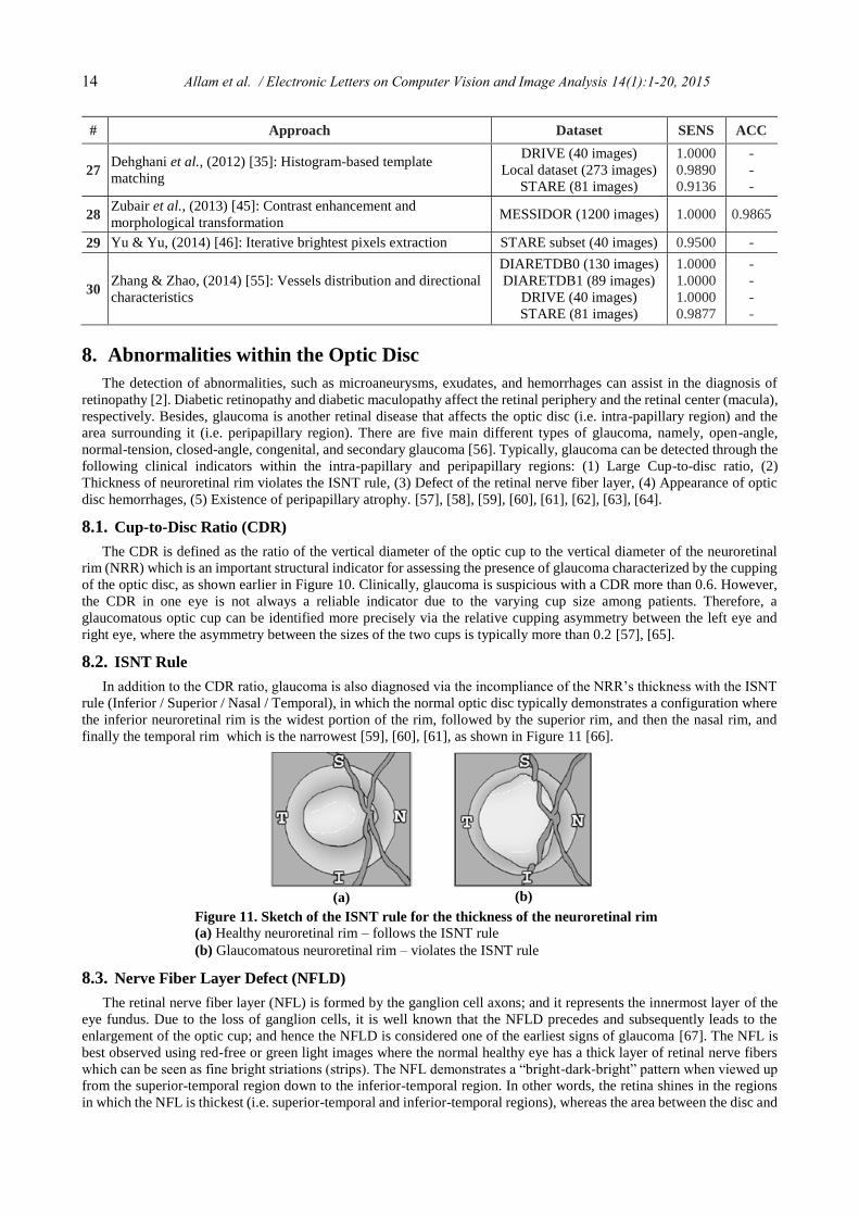
the macula (i.e. temporal region) appears darker [57], [58], [68]. Figure 12-a shows an example of the bright striations
around the superior and inferior parts in a healthy retina creating the bright-dark-bright pattern [68].
On the other hand, the region around the optic disc with NFLD gets darker and changes from stripy-texture to wedge-
shaped form. Also, blood vessels appear darker with sharp reflexes in the region of NFLD, as shown in Figure 12-b [68].
There are two kinds of NFLD, namely, localized and diffuse. The localized NFLD appears as a wedge-shaped dark
area that follows the pattern of the NFL originating from the optic disc [57], [58]. In such defects, the specificity is very
high but the sensitivity is low since these defects are a definite sign of pathology, but can occur in diseases other than
glaucoma [57]. On the other hand, diffuse NFLD can be seen in advanced glaucoma. It is usually more difficult to be
detected in one eye, but it is easily recognized when both eyes are compared together. In diffuse NFLD, there is a general
reduction of the NFL brightness causing the normal “bright-dark-bright” pattern to be lost and look like a “dark-dark-
dark” pattern (i.e. appears completely dark) [57], [58], [68].
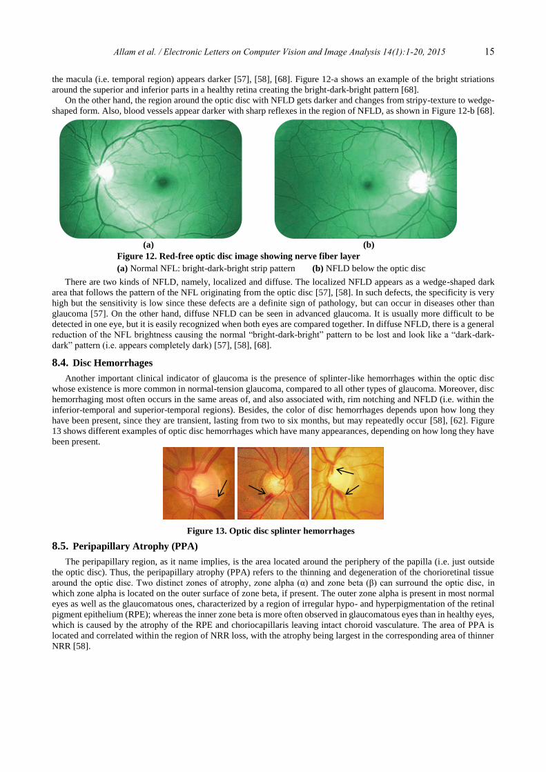
8.4. Disc Hemorrhages
Another important clinical indicator of glaucoma is the presence of splinter-like hemorrhages within the optic disc
whose existence is more common in normal-tension glaucoma, compared to all other types of glaucoma. Moreover, disc
hemorrhaging most often occurs in the same areas of, and also associated with, rim notching and NFLD (i.e. within the
inferior-temporal and superior-temporal regions). Besides, the color of disc hemorrhages depends upon how long they
have been present, since they are transient, lasting from two to six months, but may repeatedly occur [58], [62]. Figure
13 shows different examples of optic disc hemorrhages which have many appearances, depending on how long they have
been present.
8.5. Peripapillary Atrophy (PPA)
The peripapillary region, as it name implies, is the area located around the periphery of the papilla (i.e. just outside
the optic disc). Thus, the peripapillary atrophy (PPA) refers to the thinning and degeneration of the chorioretinal tissue
around the optic disc. Two distinct zones of atrophy, zone alpha (α) and zone beta (β) can surround the optic disc, in
which zone alpha is located on the outer surface of zone beta, if present. The outer zone alpha is present in most normal
eyes as well as the glaucomatous ones, characterized by a region of irregular hypo- and hyperpigmentation of the retinal
pigment epithelium (RPE); whereas the inner zone beta is more often observed in glaucomatous eyes than in healthy eyes,
which is caused by the atrophy of the RPE and choriocapillaris leaving intact choroid vasculature. The area of PPA is
located and correlated within the region of NRR loss, with the atrophy being largest in the corresponding area of thinner
NRR [58].
(a) (b)
Figure 12. Red-free optic disc image showing nerve fiber layer
(a) Normal NFL: bright-dark-bright strip pattern (b) NFLD below the optic disc
Figure 13. Optic disc splinter hemorrhages
16 Allam et al. / Electronic Letters on Computer Vision and Image Analysis 14(1):1-20, 2015
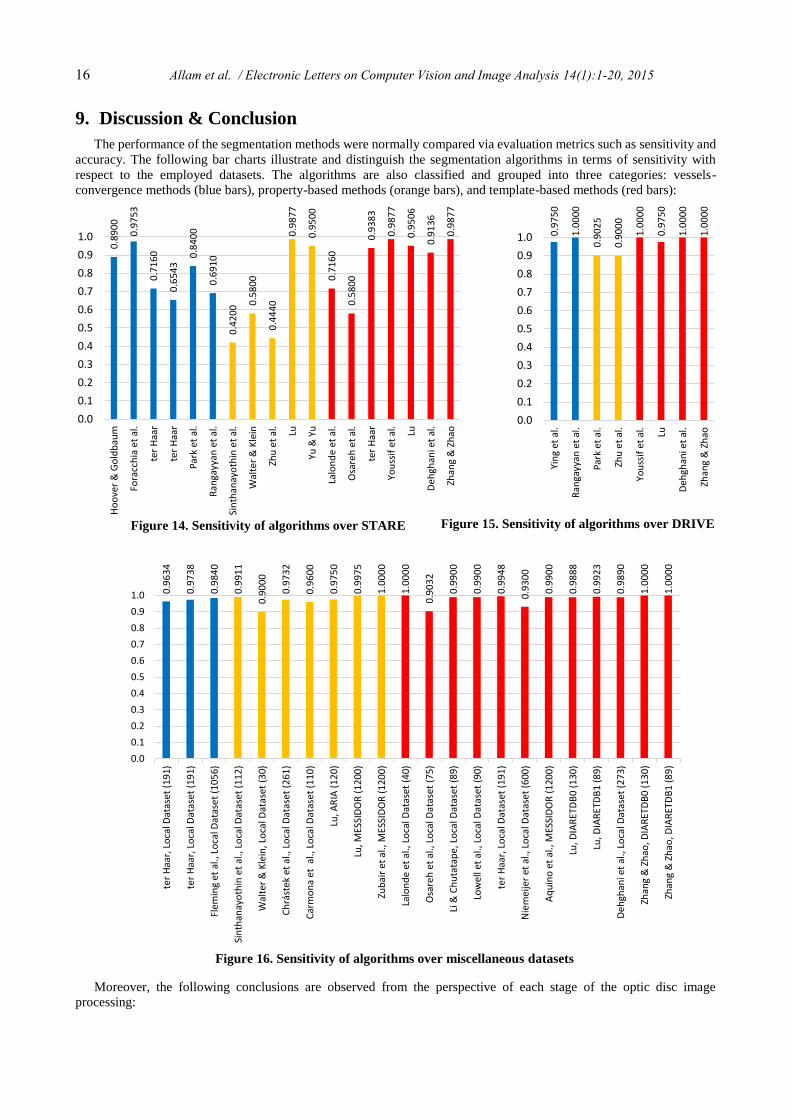
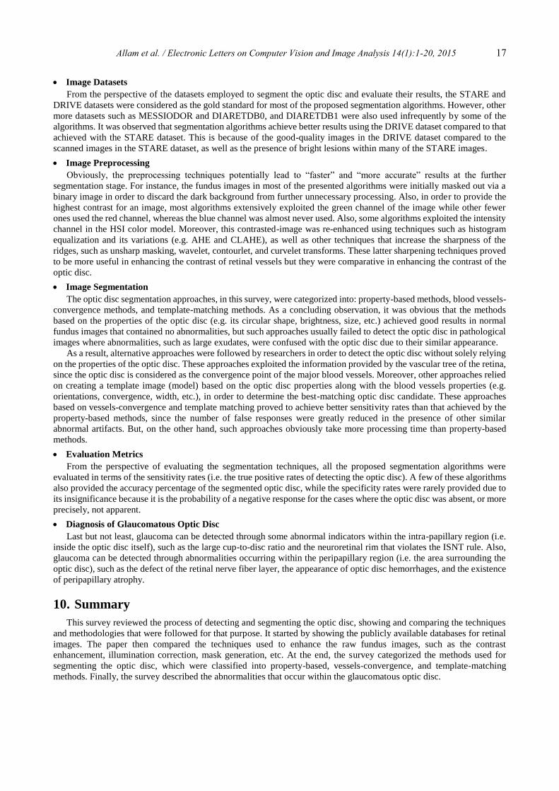
9. Discussion & Conclusion
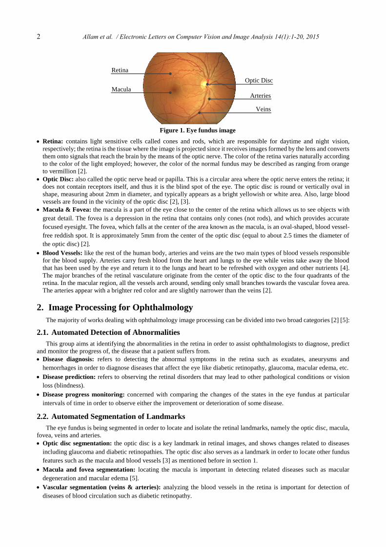
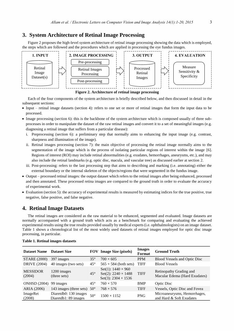
The performance of the segmentation methods were normally compared via evaluation metrics such as sensitivity and
accuracy. The following bar charts illustrate and distinguish the segmentation algorithms in terms of sensitivity with
respect to the employed datasets. The algorithms are also classified and grouped into three categories: vessels-
convergence methods (blue bars), property-based methods (orange bars), and template-based methods (red bars):
Moreover, the following conclusions are observed from the perspective of each stage of the optic disc image
processing:
0.9
75
0
1.0
00
0
0.9
02
5
0.9
00
0
1.0
00
0
0.9
75
0
1.0
00
0
1.0
00
0
0.0
0.1
0.2
0.3
0.4
0.5
0.6
0.7
0.8
0.9
1.0
Yin
g et
al.
Ran
gayy
an e
t al
.
Par
k et
al.
Zhu
et
al.
You
ssif
et
al.
Lu
Deh
ghan
i et
al.
Zhan
g &
Zh
ao
Figure 15. Sensitivity of algorithms over DRIVE
0.8
90
0
0.9
75
3
0.7
16
0
0.6
54
3
0.8
40
0
0.6
91
0
0.4
20
0 0.5
80
0
0.4
44
0
0.9
87
7
0.9
50
0
0.7
16
0
0.5
80
0
0.9
38
3
0.9
87
7
0.9
50
6
0.9
13
6
0.9
87
7
0.0
0.1
0.2
0.3
0.4
0.5
0.6
0.7
0.8
0.9
1.0
Ho
ove
r &
Go
ldb
aum
Fora
cch
ia e
t al
.
ter
Haa
r
ter
Haa
r
Par
k et
al.
Ran
gayy
an e
t al
.
Sin
than
ayo
thin
et
al.
Wal
ter
& K
lein
Zhu
et
al.
Lu
Yu &
Yu
Lalo
nd
e et
al.
Osa
reh
et
al.
ter
Haa
r
You
ssif
et
al.
Lu
Deh
ghan
i et
al.
Zhan
g &
Zh
ao
Figure 14. Sensitivity of algorithms over STARE
0.9
63
4
0.9
73
8
0.9
84
0
0.9
91
1
0.9
00
0
0.9
73
2
0.9
60
0
0.9
75
0
0.9
97
5
1.0
00
0
1.0
00
0
0.9
03
2
0.9
90
0
0.9
90
0
0.9
94
8
0.9
30
0
0.9
90
0
0.9
88
8
0.9
92
3
0.9
89
0
1.0
00
0
1.0
00
0
0.0
0.1
0.2
0.3
0.4
0.5
0.6
0.7
0.8
0.9
1.0
ter
Haa
r, L
oca
l Dat
aset
(1
91)
ter
Haa
r, L
oca
l Dat
aset
(1
91)
Flem
ing
et a
l., L
oca
l Dat
ase
t (1
05
6)
Sin
than
ayo
thin
et
al.,
Lo
cal D
atas
et (
11
2)
Wal
ter
& K
lein
, Lo
cal D
atas
et (
30)
Ch
rást
ek e
t al
., Lo
cal D
atas
et (
261
)
Car
mo
na
et a
l., L
oca
l Dat
aset
(1
10
)
Lu, A
RIA
(1
20
)
Lu, M
ESSI
DO
R (
12
00)
Zub
air
et a
l., M
ESSI
DO
R (
12
00
)
Lalo
nd
e et
al.,
Lo
cal D
atas
et (
40)
Osa
reh
et
al.,
Lo
cal D
atas
et (
75)
Li &
Ch
uta
tap
e, L
oca
l Dat
aset
(8
9)
Low
ell e
t al
., Lo
cal D
atas
et (
90)
ter
Haa
r, L
oca
l Dat
aset
(1
91)
Nie
mei
jer
et a
l., L
oca
l Dat
aset
(6
00)
Aq
uin
o e
t al
., M
ESSI
DO
R (
120
0)
Lu, D
IAR
ETD
B0
(130
)
Lu, D
IAR
ETD
B1
(89)
Deh
ghan
i et
al.,
Loca
l Dat
aset
(2
73)
Zhan
g &
Zh
ao, D
IAR
ETD
B0
(1
30
)
Zhan
g &
Zh
ao, D
IAR
ETD
B1
(8
9)
Figure 16. Sensitivity of algorithms over miscellaneous datasets
Allam et al. / Electronic Letters on Computer Vision and Image Analysis 14(1):1-20, 2015 17
Image Datasets
From the perspective of the datasets employed to segment the optic disc and evaluate their results, the STARE and
DRIVE datasets were considered as the gold standard for most of the proposed segmentation algorithms. However, other
more datasets such as MESSIODOR and DIARETDB0, and DIARETDB1 were also used infrequently by some of the
algorithms. It was observed that segmentation algorithms achieve better results using the DRIVE dataset compared to that
achieved with the STARE dataset. This is because of the good-quality images in the DRIVE dataset compared to the
scanned images in the STARE dataset, as well as the presence of bright lesions within many of the STARE images.
Image Preprocessing
Obviously, the preprocessing techniques potentially lead to “faster” and “more accurate” results at the further
segmentation stage. For instance, the fundus images in most of the presented algorithms were initially masked out via a
binary image in order to discard the dark background from further unnecessary processing. Also, in order to provide the
highest contrast for an image, most algorithms extensively exploited the green channel of the image while other fewer
ones used the red channel, whereas the blue channel was almost never used. Also, some algorithms exploited the intensity
channel in the HSI color model. Moreover, this contrasted-image was re-enhanced using techniques such as histogram
equalization and its variations (e.g. AHE and CLAHE), as well as other techniques that increase the sharpness of the
ridges, such as unsharp masking, wavelet, contourlet, and curvelet transforms. These latter sharpening techniques proved
to be more useful in enhancing the contrast of retinal vessels but they were comparative in enhancing the contrast of the
optic disc.
Image Segmentation
The optic disc segmentation approaches, in this survey, were categorized into: property-based methods, blood vessels-
convergence methods, and template-matching methods. As a concluding observation, it was obvious that the methods
based on the properties of the optic disc (e.g. its circular shape, brightness, size, etc.) achieved good results in normal
fundus images that contained no abnormalities, but such approaches usually failed to detect the optic disc in pathological
images where abnormalities, such as large exudates, were confused with the optic disc due to their similar appearance.
As a result, alternative approaches were followed by researchers in order to detect the optic disc without solely relying
on the properties of the optic disc. These approaches exploited the information provided by the vascular tree of the retina,
since the optic disc is considered as the convergence point of the major blood vessels. Moreover, other approaches relied
on creating a template image (model) based on the optic disc properties along with the blood vessels properties (e.g.
orientations, convergence, width, etc.), in order to determine the best-matching optic disc candidate. These approaches
based on vessels-convergence and template matching proved to achieve better sensitivity rates than that achieved by the
property-based methods, since the number of false responses were greatly reduced in the presence of other similar
abnormal artifacts. But, on the other hand, such approaches obviously take more processing time than property-based
methods.
Evaluation Metrics
From the perspective of evaluating the segmentation techniques, all the proposed segmentation algorithms were
evaluated in terms of the sensitivity rates (i.e. the true positive rates of detecting the optic disc). A few of these algorithms
also provided the accuracy percentage of the segmented optic disc, while the specificity rates were rarely provided due to
its insignificance because it is the probability of a negative response for the cases where the optic disc was absent, or more
precisely, not apparent.
Diagnosis of Glaucomatous Optic Disc
Last but not least, glaucoma can be detected through some abnormal indicators within the intra-papillary region (i.e.
inside the optic disc itself), such as the large cup-to-disc ratio and the neuroretinal rim that violates the ISNT rule. Also,
glaucoma can be detected through abnormalities occurring within the peripapillary region (i.e. the area surrounding the
optic disc), such as the defect of the retinal nerve fiber layer, the appearance of optic disc hemorrhages, and the existence
of peripapillary atrophy.
10. Summary
This survey reviewed the process of detecting and segmenting the optic disc, showing and comparing the techniques
and methodologies that were followed for that purpose. It started by showing the publicly available databases for retinal
images. The paper then compared the techniques used to enhance the raw fundus images, such as the contrast
enhancement, illumination correction, mask generation, etc. At the end, the survey categorized the methods used for
segmenting the optic disc, which were classified into property-based, vessels-convergence, and template-matching
methods. Finally, the survey described the abnormalities that occur within the glaucomatous optic disc.

18 Allam et al. / Electronic Letters on Computer Vision and Image Analysis 14(1):1-20, 2015
References
[1] K. Mahesh K. and K. Nilesh S., "Review on Fundus Image Acquisition Techniques with Database Reference to
Retinal Abnormalities in Diabetic Retinopathy," Int. J. Comput. Applicat., vol. 68, no. 8, pp. 17-27, 2013.
[2] X. Zhu, R. M. Rangayyan and A. L. Ells, "Digital Image Processing for Ophthalmology: Detection of the Optic Nerve
Head," in Synthesis Lectures on Biomedical Engineering, Morgan & Claypool Publishers, 2011.
[3] A. A. A. Youssif, A. Z. Ghalwash and A. A. S. A. Ghoneim, "Optic Disc Detection From Normalized Digital Fundus
Images by Means of a Vessels' Direction Matched Filter," IEEE Trans. Med. Imag., vol. 27, no. 1, pp. 11-18, 2008.
DOI: 10.1109/TMI.2007.900326
[4] Royal National Institute of Blind People (RNIB), "Retinal vessel occlusion," 7 August 2013. [Online]. Available:
http://www.rnib.org.uk/eyehealth/eyeconditions/eyeconditionsoz/Pages/retinal_vessel_occlusion.aspx. [Accessed 19
August 2013].
[5] N. Patton, T. M. Aslam, T. MacGillivray, I. J. Deary, B. Dhillon, R. H. Eikelboom, K. Yogesan and I. J. Constable,
"Retinal image analysis: Concepts, applications and potential," Progress in Retinal and Eye Research, vol. 25, pp. 99-
127, 2006. DOI: 10.1016/j.preteyeres.2005.07.001
[6] R. C. Gonzalez and R. E. Woods, Digital Image Processing, Pearson Prentice Hall, 2008.
[7] M. Goldbaum, "The STARE Project," 2000. [Online]. Available:
http://www.parl.clemson.edu/~ahoover/stare/index.html. [Accessed 28 July 2013].
[8] J. J. Staal, M. D. Abramoff, M. Niemeijer, M. A. Viergever and B. van Ginneken, "Ridge Based Vessel Segmentation
in Color Images of the Retina," IEEE Trans. Med. Imag., vol. 23, pp. 501-509, 2004. DOI: 10.1109/TMI.2004.825627
[9] MESSIDOR - TECHNO-VISION Project, "MESSIDOR," 28 March 2008. [Online]. Available:
http://messidor.crihan.fr. [Accessed 31 July 2013].
[10] J. Lowell, A. Hunter, D. Steel, B. Ryder and E. Fletcher, "Optic Nerve Head Segmentation," IEEE Trans. Med. Imag.,
vol. II, no. 23, 2004. DOI: 10.1109/TMI.2003.823261
[11] Y. Zheng, M. H. A. Hijazi and F. Coenen, "Automated ‘‘Disease/No Disease’’ Grading of Age-Related Macular
Degeneration by an Image Mining Approach," Investigative Ophthalmology & Visual Science, vol. 53, no. 13, pp.
8310-8318, November 2008. DOI: 10.1167/iovs.12-9576
[12] D. J. J. Farnell, F. N. Hatfield, P. Knox, M. Reakes, S. Spencer, D. Parry and S. P. Harding, "Enhancement of blood
vessels in digital fundus photographs via the application of multiscale line operators," J. Franklin Institute, vol. 345,
no. 7, pp. 748-765, October 2008. DOI: 10.1016/j.patrec.2006.09.007
[13] ImageRet Project, Janaury 2008. [Online]. Available: http://www.it.lut.fi/project/imageret/.
[14] E. M. Beytas, J. F. Debatin and R. A. Blinder, "Accuracy and predictive value as measures of imaging test
performance," Invest. Radiol., vol. 27, no. 5, pp. 374-378, May 1992.
[15] P. Macaskill, C. Gatsonis, J. Deeks, R. Harbord and Y. Takwoingi, "Analysing and Presenting Results," in Cochrane
Handbook for Systematic Reviews, J. Deeks, P. Bossuyt and C. Gatsonis, Eds., The Cochrane Collaboration, 2010.
[16] M. Kallergi, "Evaluation Strategies for Medical-Image Analysis and Processing Methodologies," in The Electrical
Engineering and Applied Signal Processing Series: Medical Image Analysis Methods, L. Costaridou, Ed., Taylor &
Francis Group, 2005.
[17] M. Lalonde, M. Beaulieu and L. Gagnon, "Fast and Robust Optic Disc Detection Using Pyramidal Decomposition and
Hausdorff-Based Template Matching," IEEE Trans. Med. Imag., vol. 20, no. 11, pp. 1193-1200, November 2001.
DOI: 10.1109/42.963823
[18] S. Lu, "Accurate and Efficient Optic Disc Detection and Segmentation by a Circular Transformation," IEEE Trans.
Med. Imag., vol. 30, no. 12, pp. 2126-2133, December 2011. DOI: 10.1109/TMI.2011.2164261
[19] A. Aquino, M. E. Gegúndez-Arias and D. Marín, "Detecting the Optic Disc Boundary in Digital Fundus Images Using
Morphological, Edge Detection, and Feature Extraction Techniques," IEEE Trans. Med. Imag., vol. 29, no. 11, pp.
1860-1869, November 2010. DOI: 10.1109/TMI.2010.2053042
[20] F. ter Haar, "Automatic localization of the optic disc in digital colour images of the human retina," 2005.
[21] L. Gagnon, M. Lalonde, M. Beaulieu and M.-C. Boucher, "Procedure to detect anatomical structures in optical fundus
images," in Proc. SPIE Vol. 4322, Medical Imaging 2001: Image Processing, 2001.
[22] K. A. Goatman, A. D. Whitwam, A. Manivannan, J. A. Olson and P. F. Sharp, "Colour Normalisation of Retinal
Images," Proc. Medical Image Understanding Analysis, 2003.
[23] F. A. Hashim, N. M. Salem and A. F. Seddik, "Preprocessing of Color Retinal Fundus Images," in IEEE 2013 2nd Int.
Japan-Egypt Conf. Electron. Commun. Comput., 2013. DOI: 10.1109/JEC-ECC.2013.6766410
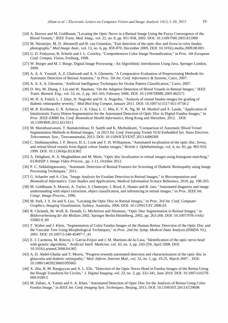
Allam et al. / Electronic Letters on Computer Vision and Image Analysis 14(1):1-20, 2015 19
[24] A. Hoover and M. Goldbaum, "Locating the Optic Nerve in a Retinal Image Using the Fuzzy Convergence of the
Blood Vessels," IEEE Trans. Med. Imag., vol. 22, no. 8, pp. 951-958, 2003. DOI: 10.1109/TMI.2003.815900
[25] M. Niemeijer, M. D. Abramoff and B. van Ginneken, "Fast detection of the optic disc and fovea in color fundus
photographs," Med Image Anal., vol. 13, no. 6, pp. 859-870, December 2009. DOI: 10.1016/j.media.2009.08.003
[26] G. D. Finlayson, B. Schiele and J. L. Crowley, "Comprehensive Color Image Normalization," in Proc. 5th European
Conf. Comput. Vision, Freiburg, 1998.
[27] W. Burger and M. J. Burge, Digital Image Processing - An Algorithmic Introduction Using Java, Springer London,
2008.
[28] A. A. A. Youssif, A. Z. Ghalwash and A. S. Ghoneim, "A Comparative Evaluation of Preprocessing Methods for
Automatic Detection of Retinal Anatomy," in Proc. 5th Int. Conf. Informatics & Systems, Cairo, 2007.
[29] A. A. S. A. Ghoneim, "Artificial Intelligence Techniques for Ocular Pattern Classification," Cairo, 2007.
[30] D. Wu, M. Zhang, J. Liu and W. Bauman, "On the Adaptive Detection of Blood Vessels in Retinal Images," IEEE
Trans. Biomed. Eng., vol. 53, no. 2, pp. 341-343, February 2006. DOI: 10.1109/TBME.2005.862571
[31] M. H. A. Fadzil, L. I. Izhar, H. Nugroho and H. A. Nugroho, "Analysis of retinal fundus images for grading of
diabetic retinopathy severity," Med Biol Eng Comput, January 2011. DOI: 10.1007/s11517-011-0734-2
[32] M. R. Krishnan, U. R. Acharya, C. K. Chua, L. C. Min, E. Y. K. Ng, M. M. Mushrif and A. Laude, "Application of
Intuitionistic Fuzzy Histon Segmentation for the Automated Detection of Optic Disc in Digital Fundus Images," in
Proc. IEEE-EMBS Int. Conf. Biomedical Health Informatics, Hong Kong and Shenzhen, 2012. . DOI:
10.1109/BHI.2012.6211611
[33] M. Maruthusivarani, T. Ramakrishnan, D. Santhi and K. Muthukkutti, "Comparison of Automatic Blood Vessel
Segmentation Methods in Retinal Images," in 2013 Int. Conf. Emerging Trends VLSI Embedded Sys. Nano Electron.
Telecommun. Syst., Tiruvannamalai, 2013. DOI: 10.1109/ICEVENT.2013.6496569
[34] C. Sinthanayothin, J. F. Boyce, H. L. Cook and T. H. Williamson, "Automated localisation of the optic disc, fovea,
and retinal blood vessels from digital colour fundus images," British J. Ophthalmology, vol. 4, no. 83, pp. 902-910,
1999. DOI: 10.1136/bjo.83.8.902
[35] A. Dehghani, H. A. Moghaddam and M. Moin, "Optic disc localization in retinal images using histogram matching,"
EURASIP J. Image Video Process., pp. 1-11, October 2012.
[36] P. C. Siddalingaswamy, "Automatic Detection of Retinal Features for Screening of Diabetic Retinopathy using Image
Processing Techniques," 2011.
[37] G. Schaefer and A. Clos, "Image Analysis for Exudate Detection in Retinal Images," in Biocomputation and
Biomedical Informatics: Case Studies and Applications, Medical Information Science Reference, 2010, pp. 198-203.
[38] M. Goldbaum, S. Moezzi, A. Taylor, S. Chatterjee, J. Boyd, E. Hunter and R. Jain, "Automated diagnosis and image
understanding with object extraction, object classification, and inferencing in retinal images," in Proc. IEEE Int.
Congr. Image Process., 1996.
[39] M. Park, J. S. Jin and S. Luo, "Locating the Optic Disc in Retinal Images," in Proc. 3rd Int. Conf. Computer
Graphics, Imaging Visualization, Sydney, Australia, 2006. DOI: 10.1109/CGIV.2006.63
[40] R. Chrástek, M. Wolf, K. Donath, G. Michelson and Niemann, "Optic Disc Segmentation in Retinal Images," in
Bildverarbeitung für die Medizin 2002, Springer Berlin Heidelberg, 2002, pp. 263-266. DOI: 10.1007/978-3-642-
55983-9_60
[41] T. Walter and J. Klein, "Segmentation of Color Fundus Images of the Human Retina: Detection of the Optic Disc and
the Vascular Tree Using Morphological Techniques," in Proc. 2nd Int. Symp. Medical Data Analysis (ISMDA '01),
2001. DOI: 10.1007/3-540-45497-7_43
[42] E. J. Carmona, M. Rincon, J. Garcia-Feijoo and J. M. Martinez-de-la-Casa, "Identification of the optic nerve head
with genetic algorithms," Artificial Intell. Medicine, vol. 43, no. 3, pp. 243-259, April 2008. DOI:
10.1016/j.artmed.2008.04.005
[43] A. D. Abdel-Ghafar and T. Morris, "Progress towards automated detection and characterization of the optic disc in
glaucoma and diabetic retinopathy," Med. Inform. Internet Med., vol. 32, no. 1, pp. 19-25, March 2007. . DOI:
10.1080/14639230601095865
[44] X. Zhu, R. M. Rangayyan and A. L. Ells, "Detection of the Optic Nerve Head in Fundus Images of the Retina Using
the Hough Transform for Circles," J. Digital Imaging, vol. 23, no. 3, pp. 332-341, June 2010. DOI: 10.1007/s10278-
009-9189-5
[45] M. Zubair, A. Yamin and S. A. Khan, "Automated Detection of Optic Disc for the Analysis of Retina Using Color
Fundus Image," in IEEE Int. Conf. Imaging Syst. Techniques, Beijing, 2013. DOI: 10.1109/IST.2013.6729698

20 Allam et al. / Electronic Letters on Computer Vision and Image Analysis 14(1):1-20, 2015
[46] C.-Y. Yu and S.-S. Yu, "Automatic Localization of the Optic Disc Based on Iterative Brightest Pixels Extraction," in
2014 Int. Symp. Comput. Consumer Control, 2014. DOI: 10.1109/IS3C.2014.166
[47] A. D. Fleming, K. A. Goatman, S. Philip, J. A. Olson and P. F. Sharp, "Automatic detection of retinal anatomy to
assist diabetic retinopathy screening," Physics in Medicine and Biology, vol. 52, no. 2, pp. 331-345, January 2007.
[48] H. Ying, M. Zhang and J. Liu, "Fractal-based Automatic Localization and Segmentation of Optic Disc in Retinal
Images," in Proc. 29th Annu. Int. Conf. IEEE Eng. Med. Biol. Soc., 2007. DOI: 10.1109/IEMBS.2007.4353247
[49] J. Park, K. N.T. and G. Lee, "Optic Disc Detection in Retinal Images using Tensor Voting and Adaptive Mean-Shift,"
in 2007 IEEE Int. Conf. Intell. Comput. Commun. Process., 2007. DOI: 10.1109/ICCP.2007.4352167
[50] R. M. Rangayyan, X. Zhu, F. J. Ayres and A. L. Ells, "Detection of the Optic Nerve Head in Fundus Images of the
Retina with Gabor Filters and Phase Portrait Analysis," J. Digital Imaging, vol. 23, no. 4, pp. 438-453, August 2010.
DOI: 10.1007/s10278-009-9261-1
[51] A. Osareh, M. Mirmehdi, B. Thomas and R. Markham, "Comparison of Colour Spaces for Optic Disc Localisation in
Retinal Images," in Proc. 16th Int. Conf. Pattern Recognition, 2002. DOI: 10.1109/ICPR.2002.1044865
[52] H. Li and O. Chutatape, "Automated Feature Extraction in Color Retinal Images by a Model Based Approach," IEEE
Trans. Biomed. Eng., vol. 51, no. 2, pp. 246-254, February 2004. DOI: 10.1109/TBME.2003.820400
[53] M. Foracchia, E. Grisan and A. Ruggeri, "Detection of Optic Disc in Retinal Images by Means of a Geometrical
Model of Vessel Structure," IEEE Trans. Med. Imag., vol. 23, no. 10, pp. 1189-1195, October 2004. DOI:
10.1109/TMI.2004.829331
[54] S. Lu, "Automatic Optic Disc Detection using Retinal Background and Retinal Blood Vessels," in 2010 3rd Int. Conf.
Biomedical Eng. Informatics, Yantai, 2010. DOI: 10.1109/BMEI.2010.5639660
[55] D. Zhang and Y. Zhao, "Novel Accurate and Fast Optic Disc Detection in Retinal Images with Vessel Distribution
and Directional Characteristics," IEEE J. Biomed. Health Informatics, no. 99, 28 October 2014. DOI:
10.1109/JBHI.2014.2365514
[56] The American Academy of Ophthalmology, 2014. [Online]. Available: http://www.aao.org/aao/.
[57] R. Thomas, K. Loibl and R. Parikh, "Evaluation of a Glaucoma patient," Indian J. Opthalmology, vol. 59, no. 7, pp.
43-52, 2011. DOI: 10.4103/0301-4738.73688
[58] M. Fingeret, F. A. Medeiros, R. Susanna and R. N. Weinreb, "Five rules to evaluate the optic disc and retinal nerve
fiber layer for glaucoma," Optometry, vol. 76, no. 11, pp. 661-668, November 2005. DOI:
10.1016/j.optm.2005.08.029
[59] L. G. Nyul, "Retinal Image Analysis for Automated Glaucoma Risk Evaluation," Proc. SPIE: Medical Imaging,
Parallel Process. Images, Optimization Techniques, vol. 7497, pp. 1-9, October 2009. DOI: 10.1117/12.851179
[60] R. R. A. Bourne, "The Optic Nerve Head in Glaucoma," Community Eye Health Journal, vol. 19, no. 59, pp. 44-45,
2006.
[61] Z. Zhang, C. K. Kwoh, J. Liu, C. Y. L. Cheung, T. Aung and T. Y. Wong, "Automatic Glaucoma Diagnosis with
mRMR-based Feature Selection," J. Biometrics & Biostatisics, pp. 1-8, 2012. DOI: 10.4172/2155-6180.S7-008
[62] Japan Glaucoma Society, Guidelines for Glaucoma, 2nd ed., Tokyo: Japan Glaucoma Society, 2006.
[63] Y. Hatanaka, C. Muramatsu, A. Sawada, T. Hara, T. Yamamoto and H. Fujita, "Glaucoma Risk Assessment Based on
Clinical Data and Automated Nerve Fiber Layer Defects Detection," in 34th Ann. Int. Conf. IEEE EMBS, San Diego,
California, 2012. DOI: 10.1109/EMBC.2012.6347352
[64] Z. Zhang, F. S. Yin, J. Liu, W. K. Wong, N. M. Tan, B. H. Lee, J. Cheng and T. Y. Wong, "ORIGA-light: An Online
Retinal Fundus Image Database for Glaucoma Analysis and Research," in 32nd Ann. Int. Conf. IEEE EMBS, Buenos
Aires, 2010. DOI: 10.1109/IEMBS.2010.5626137
[65] R. Sihota, G. Srinivasan, T. Dada, V. Gupta, D. Ghate and A. Sharma, "Is the ISNT rule violated in early primary
open-angle glaucoma - a scanning laser tomography study," Eye, vol. 22, pp. 819-824, 2008. DOI:
10.1038/sj.eye.6702798
[66] Root Eye Network, [Online]. Available: http://www.ophthobook.com/questions/question-what-is-the-isnt-rule-in-
glaucoma.
[67] C. Muramatsu, Y. Hayashi, A. Sawada, Y. Hatanaka, T. Hara, T. Yamamoto and H. Fujita, "Detection of retinal nerve
fiber layer defects on retinal fundus images for early diagnosis of glaucoma," J. Biomedical Optics, vol. 15, no. 1, pp.
1-7, February 2010. DOI: 10.1117/1.3322388
[68] T. Kubena, M. Kofronova and P. Cernosek, "Nerve Fiber Layer Defects Imaging in Glaucoma," in The Mystery of
Glaucoma, T. Kubena, Ed., InTech, 2011, pp. 187-198. DOI: 10.5772/1028